Embed Size (px)
Citation preview

HIGHWAY ACCIDENT RATES AND RURAL TRAVEL DENSITIES
HAROLD BRODSKY
Department of Geographk. L’nibersity of Maryland. College Park. >ID 111741. I..S..4
and
A. SHALOM HAKKERT
Koad Safety Center. IFrae Institute of Technolog), Haifa 3XH). Israel
Abstract-Rural highway injury accident rates should theoretically increase \vi:h an increase in travel
densities. Regression analyses of cross-sectional data on U.S. Primary and Secondary highways show a
moderate positive associatton. but on the Interstate this association appears to be invariant. Fatal accident rates, on the other hand, are negatively associated with travel densities. Explanations for these results may
be found in variables associated with travel densities. such as speed. speed variability. types of crash. and accessibility to emergency medical services. Changes in travel densities. betueen 1976 and 1979. on the
major rural highway systems have been accommodated with no apparent effect on average accident rates.
The risk of an highway accident is theoretically affected by volume of traffic, or travel density, Baker[1976]. This factor could be important-in highway safety research because accident data need to be standardized when making comparisons over time, or between locations. Empirical analyses of the effect of traffic volume on accident rates. however, have often shown inconclusive or contradictory results.
Traffic volume may affect risk for reasons that can be illustrated by a hypothetical problem: Imagine driving along a rural road without encountering another vehicle. Now imagine driving along the same road but with many vehicles on it, so that one is obliged to maneuver from time-to-time in order to pass, or to avoid collision with entering traffic. Which of the two situations presents a greater risk to the vehicle of an accident per unit distance of travel? and, why?
Consider three broad categories of highway accidents: single-vehicle, multi-vehicle, and pedestrian. The risk of a single-vehicle accident (under the simplest assumptions) should not vary with travel densities. It is possible, however, that some single-vehicle accidents are actually caused by movements to avoid collision with other vehicles, and some accidents that might have been single-vehicle, may become multi-vehicle because other vehicles happen to be in the way. One can think of still other ways that traffic might affect single-vehicle accidents.
The relationship between traffic volume and multi-vehicle accidents may be less ambiguous. All other things being equal, the possibility of a collision with another vehicle, per unit distance, traveled, would seem to increase with the number of vehicles that pass near, or by. The same may be true of pedestrian accidents. Since higher traffic areas tend to have more pedestrians, the accident rate for pedestrians may also increase with traffic volume.
Although this discussion is incomplete, we have suggested some reasons why higher accident rates might be related to higher traffic volumes. This association can be found by comparing U.S. urban and rural injury accident rates, Table 1. On both Interstate and Primary road systems, urban areas show higher injury accident rates than rural areas. A close inspection of this table, however, shows a number of inconsistencies.
The Interstate has a dramatically lower injury accident rate than the Primary system, despite higher travel densities. Unlike the injury accident rates, the fatal accident rates increase from urban to rural areas. Some obvious reasons can be suggested for these differences but the point is that the influence of traffic on accident rates is not a simple matter of ratio adjustment. Apparently the more specific one gets, the more complex the role of traffic volume may become. Still, the issue needs to be considered, and clarified, if not fully resolved.
In this paper we will examine previous studies and attempt to integrate findings. Special care
73

-1 H. BRODSKV and A. S. HARKEKT
Table 1. Comparisons of fatal and injury accident rates with densities. by highway system
Highway
sys:em
Fata !njury
Accident Accident Rate* Rate**
Travel Oensity'*'
Intersxte Urban
Rural
Primary Vrban
Rural
Secondary (no urban)
Rural
1.18 56.3 47,741
1.59 29.0 11,999
2.31 152.9 17,531
3.96 79.5 3,210
5.06 128.5 930
l
*t
t**
Source:
Fatal Accident per 100 million vehicle miles
Injury accident rates are fatal plus nonfatal injury accidents per 100 million vehicle miles
Travel Densities are in daily vehicle miles permile
"Fatal and Injury Accident Rates on Federal-Aid and other Highway !iystems/1978." U.S. Department of Transportation May, 1980, page 1.
will be needed because of the variety of geographic and temporal data units that have been used. Interpretation is also clouded by a potentially serious problem in statistical bias. We will take these factors into consideration when we present the results of our analysis.
DEFINITIONS
The term traffic volume, as used here, is related to the term travel density. Traffic volume is average daily travel (ADT), usually measured by a counter placed across a road. A sample of ADTs can be used to estimate annual vehicle-miles for a length of highway, or highways, in an area. Travel densities are annual vehicle-miles per mile. Traffic volume, therefore, is a measure of the flow of vehicles at a specific location, while travel density is a measure of the flow of vehicles within a region.
The term accident in this paper may refer to all recorded highway collisions including property damage only. Injury accidents relate more specifically to accidents where bodily harm is reported, and fatal accidents are only those resulting in one or more fatal injuries. Accident data, and injury accident data are subject to inaccuracies due to subjectivity in reporting, and incomplete reporting. Fatal accident data are subject to less error. All rates mentioned here are based on using vehicle-miles, or vehicle-km, as a standardizing denominator.
PREVIOUS STUDIES
In their study of rural highways in several U.S. states, Kihlberg and Tharp[ 19681 found that, in general, single-vehicle accident rates decreased with volume but that multi-vehicle accident rates increased. Total number of accidents, the sum of the two groups, rose at a faster rate than traffic volume in several, but not all, of their analyses. Injury and property damage accidents behaved similarly with respect to traffic volume, but their samples were too small to generalize about pedestrian, or fatal accidents.
On the other hand, Pfundt(19691 reported that total accident rates decreased (rather than increased) with traffic volume. In Denmark the decrease was 30% (in Germany, 15%), per 100% increase in volume. Pfundt doubted, however, if these aggregate figures would be useful in accident studies, and recommended instead that traffic volume at the time of the accident be used.
In his more detailed hourly studies he showed that the association between accident rates and volume was not monotonic but “U” shaped. During low density periods (usually at early

Highway accident rates and rural trawl drnsiries 'i
hours of the day) accident rates were high. They decreased at medium densities only to rise again at high densities.
In an evaluation of road accidents and traffic volume in Israel, Ceder and Livneh [ 19781 used both cross-sectional and time-sequence anaIyses. In their cross-sectional models. seven out of eight regressions for two-lane highways showed an increase in accident rate with volume. On four-lane divided highways, however, the relationship differed: six out of eight regressions showed a decrease in accident rate with an increase in ADT. The time-sequence analyses consistently showed a decrease in accident rates with an increase in traffic volume.
Chatiield’s[l970] study of the Interstate system in the US. was concerned only with fatal accidents. His downward sloping curves indicated an increase in average rurai fatal accident rates with a decrease in travel densities.
The inconsistencies between these studies may be partly due to the variation in the units of aggregation used: temporal vs spatial; hourly vs annual; or 0.3 mile road segments vs states. Differences are also apparent by severity of accident: injury vs fatal. However, another problem may lie in the accuracy of the data, and the statistical technique used. Regression analyses that associate accident rates with traffic volume, or travel densities, contain a common component on both sides of the equation-explicitly, or implicitly. Generally, such analyses have been viewed with suspicion, although for reasons that were not made clear until recently, Long[ 19791.
The mathematicaf forms used by Pfundt, and by Ceder and Livneh (and in our own analyses) are power functions:
Accidents x lO”i(km X ADT x 365) = ~I(ADT)~.
The denominator of the dependent variable, is accidents per vehicle-km, or annual accident rate, The independent variable is traffic volume measured by average daily travel (ADT). The common component is, therefore, ADT. The parameters a and p can be estimated by linear regression if accident rate and ADT are expressed in logarithms:
Log (Accident rate) = Log a + p Log (ADT).
Kihlberg and Tharp used a different mathematical form:
Log (Accidents) = Log a + b 1 Log (ADT) +- b2 Log (Length) (3)
Length refers to a highway section with uniform ADT along which accidents are counted. In their analysis, highway sections were conveniently chosen at lengths of 0.3 miles so that the relationship could be simplified. When highway length is made uniform it no longer has a measurable effect on accident variation and can be dropped from the regression model. In the formula (3) a value greater than one for b 1 indicates an increasing accident rate with traffic volume.
Although ratios are not explicit in eqn (3), the form is mathematically related to eqn (2) because bl is equal to (p + I). In (3) the dependent variable is accidents per length. In (2) the dependent variable is accidents per length times ADT. Shifting ADT in (2) to the right side of the equation results in p Log (ADT) + Log (ADT), or (p t I) Log (ADT).
Chatfieid’s regression model used an unusual formulation based on hyperbolic curves. However, his Y variable (fatal accident rates), and his X variable (travel densities) also contain a common component, vehicle-miles. In fact, since accident rates and traffic volume, or travel densities, are meaningful ratios whose estimated relationship is the purpose of the analysis there is no real way to avoid the pesky issue of common component regression.
Regressions involving ratios with a common component, occur, from time-to-time, in other areas of highway safety research. For example, fatal accident rate may be correlated with an index of law enforcement, such as traffic tickets per fatal accident. A standardization such as accidents per pedestrian may be correlated with another standardization, pedestrians per vehicle-kilometer. If the theoretical reasonableness of these ratios is not in doubt, then there is no reason to expect biased results, provided the common component is measured without error.

‘h H. BRODSRY and A. S. HNKERT
If errors do occur in the common component they will be correlated. The slope of a regression will have a negative bias if the common component occupies opposite positions in the ratios-as they do in all of the traffic volume, or travel density, studies above.
Is it possible then, that some of the empirical findings which show a decreasing accident rate with traffic volume. or density. are due to a statistical bias? Since all measurements of volume or density are based on samples, they are inherently subject to error, although Cleveland[ 1976] stated that standard errors of less than 10% have been recorded for roads with ADTs of greater than jO0 vehicles per day. The exact amount, or form of error in the studies above. however, are unknown and, therefore. there is no direct way to determine how much this bias has affected the results. In our analysis, we will perform a series of simulation experiments to estimate the sensitivity of our data to this bias.
DATA.4GGREGATION
The major source of data used here comes from the annual series (beginning in 1967) “Fatal and Injury Accident Rates on Federal-Aid Highway Systems”, published by the U.S. Depart- ment of Transportation. In this series, data are tabulated into urban and rural components by major highway systems, but are only available at a state level of aggregation,
For purposes of developing generalizations applicable to national safety policy, state level data would seem to be appropriate because they are comprehensive. Most safety research, however, is concerned with small areas, or even specific sites, and there may be some question as to whether a relationship appearing at a state level of aggregation may also apply to more detailed levels of analysis.
In certain circumstances state level data may actually provide a more accurate estimate of the effect of travel density on accidents than smaller area data. For example, suppose age of driver varies significantly from county to county, and in such a way that the higher density counties tend to have a higher proportion of teenage drivers. Age of driver might be needed as an additional independent variable to obtain an unbiased estimate of the effect of travel density. Between states, however, variation in average age of driver may be unrelated to average state travel density. If so, leaving out age as a variable in state data will not bias the trend.
Matters do not always work out simpler at higher levels of aggregation. State level data
might require the introduction of new variables whose specification at lower aggregation levels would have been unnecessary. For example, suppose higher travel density states tend to have stricter licensing and auto inspection laws than do lower travel density states. Failure to consider this variable may distort the relationship.
The possible omission of an explanatory variable related both to independent and dependent variables is, therefore, the main problem in making inferences from one level of areal unit to another. Other technical aspects of this problem are discussed in the literature on ecological correlation, Langbein and Lichtman[ 19781.
The data in this study are not only highly aggregated by geographic level, but similarly, by time interval. Variations due to hourly, weekly, or seasonal cycles are smoothed out in the yearly averages. Care should also be used when making inferences from yearly averages to smaller units of time.
Generally, researchers prefer to work with data from small geographic areas, or specific intervals of time, because they can select road sections or periods that are reasonably homogeneous. This strategy of data collection is designed to reduce confounding errors by approximating experimental conditions. The price paid for this convenience, however, lies in a reduction in the number of accident occurrences. For fatal accidents, area1 units of less than state size, or less than a year, often have too much variability for reliable regressions.
ANALYSIS
In our earlier discussion we suggested that accident rates should rise with increases in travel densities, provided there are no confounding variables. To test this relationship we used the power model, eqns (1) and (2), with rural injury and fatal accident rates, by state, for the Y variable, and travel densities, by state, as the X variable, Fig. 1, Tables 2 and 3. On Primary and Secondary highway systems injury accident rates were positively associated with travel

Highway accident rates and rural travel densities
. .
l
-1.80 - . . correlation cucfficitnt
-1.35 - l
l
l l . -2.10 - . .
.
. -2.25 -
.
-2.4il - l
I I t I I I I I I I t I I I
.I8 .36 54 72 90 1 08 I 26
1°f10
Vehicle.Miles
Miles >
DENSITY
Fig. I. Relationship between fatal accident rate and travel densities. Interstate. 1977-78.
Table 2. Regression analyses of injury accident rates and travel densities by rural highway system
Highway Intercept * system (a)
Regression * Coefficient
(b)
Correlation Coefficient
(r)
.029
-.I21 .233 .369 (.152) C.092)
Secondary (1978)
N = 41
,156 .219 ,358 (.I911 (.091)
Source: Data from "Fatal and Injury Accident f?ates" U.S. Dept. of Transportation, Feb., 1980 and May, 1980.. pages 2 and 23.
* Form of equation:
Loglo (Injury Accident Rate) =
LoglOa + b Loglo (Density)
Injury accident rate is fatal plus non-fatal accidents per 100 million vehicle miles. Density is vehicle-miles per mile. N = sample size.
Standard errors in parenthesis.

-Y H. BRODSKY and A. S. H.XKERT
Table 3. Regrsss~on analysss of fatal accident rates and travel densities by rural highway system
;iignway System
:ntercept*
(a)
Regression* Coefficient
(b)
Correlation Coefficient
(r)
interstate (1977-1978)
N = 48
-1.633 -.372 -.401 (.204 ) C.125)
Primary (1978)
N = 43
-1.400 (.096 )
-.218 -. 505 t.058)
Secondary ( 1978)
N -41
-1.369 (.168)
-.oat c.081)
-.158
Source: Data from, "Fatal and Injury Accident Rates" U.S. Department of Transportation, February, 1980 and May, 1980, page 2
l Form of equations:
Loglo (Fatal Accident Rate) =
LoglOa + b Loglo (Density)
Fatal accident rate is fatal accidents oer 100 million miles Density is'vehicle-miles per mile. N = sample size
Standard errors in parenthesis.
densities. The associations, however, were not strong, and injury accident rates may be invariant with travel densities on the Interstate.
For fatal accident rates the trends are different. The associations are consistently negative. Similar negative relations appear in Chatfield’s 1967-68 Interstate analysis and in regressions we made on several highway systems with 1974-75 data. Apparently the trends are persistent.
These regressions, however, are biased, to some degree, toward a negative association. Since we know neither the magnitude, nor the precise nature of the errors involved in estimating state highway vehicle miles, we have no way of determining the unbiased relation- ships. What we can do, however, is subject the data to an addition of a random normal error in vehicle-miles, recompute the regressions, and estimate the sensitivity of the data to correlated
errors. In our simulation experiments we assumed that vehicle-miles were neither consistently over
nor underestimated, that error was proportional to size, and normally distributed. We estimated that a standard error in the measurement of vehicle-miles of 20% would be as large as we would need to consider here. For each level of error we ran thirty trials. Normal random numbers, with a mean of zero, and a standard deviation equal to one were multiplied by a percent error in the data and added to it. Depending on the random number, the error could be plus or minus. A state like Maine, for example, with 770 million vehicle-miles would register figures between 616 and 924 million vehicle-miles in about 68% of the trials in a simulation geared to a 20% standard error.
As can be seen from the average simulated errors in the Interstate system, a consistent negative bias in correlation and regression appears as the magnitude of the error in vehicle- miles increases, Tables 4 and 5. Our perception, however, is that even with fairly large errors in vehicle-miles this bias is unlikely to change our estimates of the relationship between injury or fatal accidents, and travel densities. Similar simulation results were obtained with Primary and Secondary highway systems.
Another measurement, accident severity (the ratio of fatal to injury accidents) in the three highway systems, is consistently negative in relation to densities, Table 6. Severity regressions

Highway accident rates and rural travel densities ‘9
Table 4. Effect of adding error to vehicle-miles in Injury accident density correlat:on. rural Interstate highway
1977-X. Mean of thirty simulations
Added * Intercept l * Error (a)
Regression ** Coefficient
(b)
Correlation Coefficient
(r)
No added error -.527 -.ozo -.029
5% -.522 -.026 C.011)
-.037 C.017) (.024)
104 -.509 -.049 -.069 (.025) C.033) (.045)
15% -.478 -.087 -.120 C.031) (.049) (.066)
20% -.438 -.145 -.I91 (.042) c.064) t.083)
l
**
percent of vehicle-miles times random normal error with mean of zero and standard deviation of one.
LogI (Injury Accident rate) =
LoglOa + b LogI (Density)
Injury accident rate is fatal plus non-fatal accidents per 100 million vehicle-miles.
Density is vehicle-miles per mile.
Standard deviation in parentheses.
Table 5. Effect of adding error to vehicle-miles in fatal accident density correlation, rural Interstate highway,
1977-78. Mean of thirty simulations
Added* Error
Intercept**
(a)
Regression** Coefficient
(b)
Correlation Coefficient
(r)
No added error -1.633 -.3?2 -.401
5% -1.631 -.375 -.402 l.011) (.Oli3) (.OZD)
10% -1.622 -.38? -.416 (.022) l.036) C.031)
15% -1.606 -.4D9 -.439 (.032) C.052) C.045)
20% -1.583 -.442 -.472 C.043) l.068) c.058)
l
l *
Percent of vehicle-miles times random normal error with mean of zero and standard deviation of one.
Loglo (Fatal Accident Rate) =
LoglDa + b Loglo (Density)
Fatal accident rate is fatal accidents oer 100 million vehicle- miles. oehsity is vehicle-miles per mile. Standard deviation in parentheses.
are not subject to the common component bias. The effect of errors in vehicle-miles in these regressions will only attenuate the negative slopes rather than increase them, Blalock[1965]. The severity trends are, therefore, conservative estimates of decline with increased travel density.

Interstate 1978
N = 48
-1.106 -.352 -.431 c.1781 (.:09i
Primary 1978
zi = 43
1.280 (.14if
Secondary 1978
N = 41
-1.525 -.300 -.418 (.218) (.104)
Source: See Table 3
* Loglo (Severity) =
LoglOd + b LoglO (Oensity)
Severity is the ratio of fatal to fdtal and injury accidents.
Density is vehicle-miles per mile.
Standard errors in parenthesis.
DISCUSSION
The positive associations of injury accident rates with travel densities on the Primary and Secondary highway systems may be due to increases in pedestrian and multi-vehicle accident rates. On divided highway and limited access highway systems such as the Interstate, however, head-on multi-vehicle accidents, and pedestrian accidents are minimized. Also, according to Baker [ 19761, same directional multi-vehicle collisions depend on “the variance of speed among vehicles moving in the same direction”. On the Interstate system, variability of speed is negatively associated with travel densities, Fig. 2. This factor along with a generally reduced multi-vehicle and pedestrian crash rate may lead to an invariant injury accident rate with travel densities on the Interstate.
Fatal accident rates on the Interstate and other systems are negatively associated with travel densities. As a result, severities increase with travel densities, and this requires some explana- tion. The first variable that may come to mind is speed. A good deal of evidence has accumulated to indicate that enforcement of the 55 mph speed limit saves lives (Tofany[l981~). As shown here, on the Interstate system, states with 60 mph as their 85 percentile speed had a ratio of 2.7 fatal accidents per 100 injury accidents, while states with 65 mph as their 85 percentile speed had 6.1 fatal accidents per 100 injury accidents, Fig. 3.
Speed may not, however, fully explain the higher fatal accident rates on the Interstate. When the 85th percentile speeds were regressed against travel densities the correlation was not signi~~ant (-0.183). On the other hand, the six leading states in fatal accident rates al1 had above average speeds at the 85th percentile. Speed appears to be a contributing factor to higher severities in some low density states, but there may be room for additional explanations.
Two factors warrant discussion here because they may have broader implications for accident research and policy. First, the type of fatal accident (first harmful event) varies with travel densities. The proportion of fatal accidents that result in overturning, increases con- siderably as travel densities decrease, Table 7. Overturning accidents are estimated to be among the most severe. Possibly conditions in low travel density states are especially hazardous for this kind of accident, and this may help to account for the higher total fatal accident rates in lower travel density states. Standardized data show, however, that several types of fatal accident rates (except pedestrian) increased with decreasing travel density, Table 8. Type of accident cannot, therefore, entirely account for higher fatal rates in louver density states.

Highkay accident rates and rural travel densities
900
315
.
.
I 1 I I I I I I I I I I I I
075 150 225 300 375 ,150 525 600 575 150 825 900 315 I 05
L"31D (
Vehicle Miles Miles >
DENSITY
Fig. 2. Relationship between variability of speed and travel densities. rural Interstate. 1977-78
IO - . .
. .
3- .
7 -
6. - csrrclatinn coefficient
5- .
. 4 - . .
. .
.
. .
I 1 I I 1 I I I I I I I I I I
53.25 (0.00 60.75 61.50 62.*5 63.66 63'75 61.56 65'25 66.06 66.75 67.50 '6.*5 66.60
Arcrage 85th Percentile Speed
Fig. 3. Relationship between severity of accident and excessive speeds as measured by average speed at the 85th percentile, rural Interstate. 1977-78.

82 H. BRODSKY and ;\. S. HAI;KERT
Tabls “. Variation in percent OF fatat kdcnts by tl;ps. and m\:i densities
Travel Percent of Fatal Accldeots Densities*
(Group of States) I nultivehic’e Pedestrian Fixec Cbject
Less than 2,500
2,500 - 4,499
4.500 - 8,500
Greater than 8.505
i
Overturning
Number of Fatal
Accidents
217
Source: FARS file Interstate, 1978
* Daily Vehicle-hiles per wile
Table 8. Variation in fatal accident rates by type. and travel densities
Travel Densities*
(Group of States)
Fatal Accideot Rates**
Multivehicle Pedestrian Fixed Object
6.2
4.7
4.4
3.5
Overturning
7.7
4.2
2.4
0.2
Source: FARS file Interstate, 1978
* Daily Vehicle-miles per mile
** Fatal Accidents per 1,000 million vehicle miles
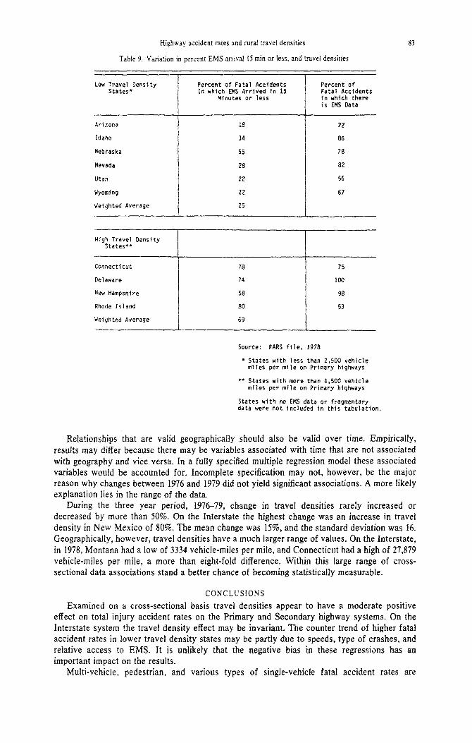
Another variable associated with travel densities is emergency medical services (EMS). Generally, it takes longer to discover, report, and rescue a traffic accident victim in a state with low rural travel densities. In lower travel density states an average of only 25% of the ambulances arrive within 15 min of the time of the fatal accident. In higher density states the average is 69% , Table 9. If rapid access to treatment saves lives then the chances that a serious injury will become fatal is more likely in a lower travel density state. This variable along with others could help to explain the increased fatal accident rate with decreased travel densities.
CHANGE OVER TIME
In 1976 a uniform functional CIassification of the principle highway systems in the United States went into effect. We were, therefore, able to regress percent change in fatal and injury accident rates, by staie, between 1976 and 1979, against percent change in travel densities. We did this for the Interstate, Primary, and Secondary rural highway systems. AI1 the regressions, however, showed non-significant, invariant results.
Highway accident rates and rural travel densities
Table 9. Variation in percent EMS arrival 15 min or less, and travel densities
83
Low Travel Density States*
Percent of Fatal Accfdents In which E!G Arrfved in 15
Minutes or less
Percent of Fatal Accidents in which there is EMS Data
Arizona 18 72
Idaho 34 86
Nebraska 55 78
Nevada 28 82
Utah 22 56
CIyoming 22 67
Weighted Average 25
High Travel Density States**
Connecticut
Delaware
New Hampshire
Rhode Island
Ueighted Average
I
78 75
74 100
58 98
80 53
69
Source: FARS file. 1978
* States with less than 2.500 vehicle miles per mile on Primary highways
** States with more than 4.500 vehicle miles per mile on Primary highways
States with no EMS data or fragmentary data were not included in this tabulation.
Relationships that are valid geographically should also be valid over time. Empirically, results may differ because there may be variabfes associated with time that are not associated with geography and vice versa. In a fully specified multiple regression model these associated variables would be accounted for. Incomplete specification may not, however, be the major reason why changes between 1976 and 1979 did not yield significant associations. A more likely explanation lies in the range of the data.
During the three year period, 1976-79, change in travel densities rarely increased or decreased by more than 50%. On the Interstate the highest change was an increase in travel density in New Mexico of 80%. The mean change was 15%. and the standard deviation was 16. Geographically, however, travel densities have a much larger range of vaIues. On the Interstate, in 1978, Montana had a low of 3334 vehicle-miles per mile, and Connecticut had a high of 27,879 vehicle-miles per mile, a more than eight-fold difference. Within this large range of cross- sectional data associations stand a better chance of becoming statistically measurable.
CONCLUSfONS
Examined on a cross-sectional basis travel densities appear to have a moderate positive effect on total injury accident rates on the Primary and Secondary highway systems. On the Interstate system the travel density effect may be invariant. The counter trend of higher fatal accident rates in lower travel density states may be partly due to speeds, type of crashes, and relative access to EMS. It is un~ikeIy that the negative bias in these regressions has an important impact on the results.
Multi-vehicle, pedestrian, and various types of single-vehicle fatal accident rates are

84 H. BRODSKY and ‘4. S. HAKKERT
affected by travel densities. This factor should be taken into account when comparing the rates of various kinds of crashes in different locations.
Changes in total fatal and injury accident rates over time (1976-79). were not perceptibly affected by changes in travel densities. Apparently, modest increases in travel densities have been accommodated on rural highways without a significant impact on average total accident
rates.
REFEREYCES
Baker J. S.. Traffic accident analysis. Transportation and Trafic Engineering Hdndbook (Edited by .I. E. Baerwald). Chap. 9. D. 388. Prentice Hall, Enalewood Cliffs. New Jersey, 1976.
Blaldck H. M.. Some implications of random measuremknt error for causal inferences. Am. J. Sociology 71. 3737. 1965. Chatfield B. V.. Relationship of fatality rates to travel densities on the interstate system. Public Roads 36. 1849. 1970.
Ceder ‘4. and Livneh M.. Further evaluation of the relationships between road accidents and average daily traffic, Accid. AnaIy. & Prep. 10. 95-109. 1978.
Cleveland D. E.. Traffic studies. Transportalion and Trafic Engineering Handbook (Edited by J. E. Baerwald). Chap. IO. p,
412. Prentice Hall. Englewood Cliffs, New Jersey, 1976. Kihlberg J. K. and Tharp K. J., Accident Rates as Related to Design Elements of Rltraf Highways. Report 48. Highway
Research Board. Washington. D.C.. 1968. Langbein L. I. and Lichtman A. J.. Ecological Inference. Sage University Paper series on Quantitative Applications in the
Social Sciences, 07-010. Sage Publications. Beverly Hills and London. 197s. Long S. 9.. The continuing debate ever the use of ratio variables: facts and fiction. Sociologicnf Methodology. 1980
(Edited by K. F. Schuessler). pp. 37-67. Jossey-Bass. San Francisco, 1979. Pfundt K.. Three difficulties in the comparison of accident rates. Accid. Anal. Sr Prer. 1. 253-39. 1969. Tofany V. L., Life is best at 55. Trajic Quart. 35. S-19, 1981.