Relationship of Rural Highway Geometry to Accident Rates in Louisiana OLIN K. DART, JR., and LAWRENCE MANN, JR., Louisiana State University

The purpose of this project was (a) to determine which geometric variables contribute most to accidents, and (b) to predict the accident potential of a certain section of Louisiana highways. This study involved approximately 1,000 miles of rural highways distributed eveply throughout Louisiana. The accident records investigated cover a 5-year period from 1962 to 1966. The variables studied in order to find their relation to accidents were percentage of trucks, traffic volume ratio, lane width, shoulder width, pavement cross slope, horizontal alignment, vertical alignment, percentage of continuous obstructions, marginal obstructions per mile, and traffic access points per mile. These 10 variables, their squares, and their first order interactions were used in a regression analysis to construct mathematical models to determine the contribution of the vari­ables to total accidents, accidents on wet roads, accidents on dry roads, accidents during the day, accidents during the night, total injuries, and total fatalities. One mathematical model shows that a total of approxi­mately 46 percent of all accidents are explained by the 10 variables in­cluded in this study. The variables not inv~stigated-involving the driver, the vehicle, and other geometrics-account for the remainder of the vari­ation in total accidents. Based on their interaction with traffic volume, the 2 geometric variables having the most important effect on accident rates are pavement cross slope and traffic conflicts. The remaining geo­metric variables studied in order of decreasing effect on accident rates are lane width, horizontal alignment, and shoulder width.

•FOR SEVERAL YEARS Louisiana has found itself in the unenviable position of pos­sessing the highest motor vehicle accident fatality rate in the nation. Table 1 gives the trend for a 10-year pei·iod from 1957 through 1966. Particularly alarming is the rate of increase in accidents and fatalities between 1962 and f 966.

In designating the cause of accidents, most authors cite 3 principal factors-the driver, the vehicle, and the roadway. In one concept, recently recalled by Baldwin (2), each accident is assigned a primary cause that results in 75 percent of all accidents -being caused by driver failure, 10 percent by vehicle deficiencies, and 15 percent by highway deficiencies. However, Baldwin goes on to discuss the more probable situa­tion that any accident is caused by an interaction of the 3 principal factors:

... If it is possible to hazard a guess, it seems likely that the driver as a cause might show up in from 80 to 90 percent of accidents, but that the highway would also appear in 40 to 50 percent of the cases and the vehicle in a somewhat smaller percentage (but certainly larger than the com­monly quoted ten percent). By the very nature of the concept, there would of course be many accidents in which causal factors might be identified in each of the three general categories. This would merely mean that more than one type of countermeasure might be useful in terms of ac­cident prevention.

Paper sponsored by Committee on Operational Effects of Geometrics and presented at the 49th Annual Meeting.

1

2

TABLE 1

LOUISIANA HIGHWAY ACCIDENTS AND ENFORCEMENT FROM 1957 TO 1966

Rura l Rural Automobile DeaU1 Rn le Hazardous Ratio or Year

Accidents Fatalities Fatalities per C:itations Citations 100 mvm to Accidents

1957 17 ,052 568 817 7 .3

1958 16,301 608 845 7.4

1959 16,972 500 603 7 .2 4~.~01 2.68

1960 15,623 594 841 7 .4 51,699 3.31

1961 15, 732 576 779 6.7 63,351 4.02

1962 17 ,299 546 770 6.4 71,876 4.16

1963 19,638 624 846 8.3 67 ,017 3.41

1964 23,934 791 1,037 9,7 68,667 2.82

1965 25,904 857 1,106 9.0 78,992 3.05

1966 29,916 917 1,232 9.4 89,061 2.98

aAccidents per 100 million vehicle-miles

A large part of Louisiana's problem may be caused by the driver in that enforce­ment has not been maintained at a sufficient level in recent years (Table 1). Authori­ties say that a 6 to 1 ratio of moving violation citations to total accidents is a minimum for effective control. Louisiana's ratio has generally ranged from between 2.6 and 4.2 to 1 in the 8-year period shown.

Nevertheless, Baldwin's point is well taken, and we resolved to pursue all available avenues of attack, including an elevation of highway deficienceis. This paper describes the work done on the project initiated in 1966 and includes the analysis, results, con­clusions, and recommendations having to do with the rural highway system in Louisiana. The purpose of the research was (a) to determine what continuous type of geometric highway design variables may be contributing most to the large traffic accident and death toll that exists in Louisiana, and (b) to predict accident potential and geometric design ·parameters. Prediction is the elusive goal here. Unless accidents can be pre­dicted above the level of chance, the processes that cause accidents cannot be under­stood with any degree of confidence.

Miller (23) reports that traffic accidents were responsible for an estimated total economic loss of $11 billion in the United States in 1967. Thus, there is that much reason, strongly reinforced by humane considerations, to gain a better understanding of the causes of highway accidents so that we may reduce their frequency and the dis­tress they cause.

The highway itself is an important determinant of where accidents happen (35). Road­way elements or characteristics, therefore, can provide an effective means for pre­dicting accident "proneness" of a given roadway. The purpose of this research was to estimate the true liability of the highway itself in causing accidents and to assess the proportionate share of liability that individual physical highway characteristics should bear.

PREVIOUS STUDIES

The literature contains many items dealing with investigations of the relationship of highway design features to highway accidents. One publication alone summarizes the findings of several hundred references (35).

Some previous resea1·ch dealt with the problem in its entfrety (7, 9, 12, 30) ; other research was limited to one variable such as shoulders or a group-offactor$(3, 5, 14, 29). In reviewing the material available, the authors limited their search to studTes­that dealt more directly with the problem under investigation. Some of the most perti­nent findings of previous research are briefly summarized in the following discussion .

3

In 1953, Raff (30) presented his findings on a study to find how accident rates on main rural highways are affected by design features and use characteristics. The fac­tors studied include number of lanes, average daily traffic (ADT), degree of curvature, pavement and shoulder widths, frequencies of curves and other sight-distance restric­tions, percentage of intersection traffic on the minor road, and many others. Surpris­ingly, Raff concluded that a number of roadway features, including grade and frequency of curves, do not appear to have any consistent effect on accident rates. He also found, as would be expected, that traffic volume and sharp curves seem to cause accidents. Wide pavement and shoulders encourage safety on 2-lane curves. Raff mentions that the most striking feature of his study was the amount of irregularity in most of the re­sults, but he adds that the principal cause is probably the tremendous complexity of the problem itself. The very complexity of the problem dictates that the data should be as homogeneous as possible. This can only be accomplished by having only one reporting agency furnish all the data. The authors have tried to do this by using data from one state.

Blensly (5) found a significant relationship between increased accident frequency and increased paved shoulder width. He states that "the results of this study should be interpreted with extreme caution, inasmuch as the traffic volumes on the bulk of the sections were less than 5,000 vehicles per day. 11 Two different approaches were taken in his study. Correlation procedures were used to evaluate the relationship between paved shoulder width and accident occurrence, and variance measures were employed to analyze the difference between the average accident frequency on sections with nar­row paved shoulders ( 4 ft or less) and the average accident frequency on sections with wide paved shoulders (8 ft or more). The analysis of covariance procedu1·es estab­lished that, when the effect of ADT was controlled, the mean number of property dam­age and total accidents was significantly higher on sections with wide paved shoulders than on sections with narrow paved shoulders in the 1,000 to 5,600 ADT range.

Belmont (3) found a similar relationship between personal injury accident frequency and paved shoulder width on sections ranging in volume from 2,000 to 12,000 vehicles per day. Belmont concluded that "apparently the advantages of wider shoulders are more than offset by tendency of drivers to be less careful. As shoulder width increases, drivers may gain an unjustified feeling of security. 11 This theory is one possible ex­planation for the relationship found in his study. Clearly, this is a startling result. Another explanation can possibly be found in the way that Blensly attenuated his data. In order to obtain a sufficient number of sample elements, he multiplied each 1-mile section of rural 2-lane highway, which was level and tangent and had paved shoulders, by the number of full years for which accident data were available after the paved shoulders were constructed.

Moskowitz (26) and Crosby (10) investigated the relative safety of various existing types of medialldesigns. .Although the research described did not include an analysis of medians, the refere.nces are included for continuity.

Schoppert's investigation (31) describes research by the Oregon State Highway Com­mission to develop equations that can be used to predict accidents on rural 2-lane high­ways from roadway elements such as ADT, lane width, shoulder width, sight-distance restrictions, commercial and residential driveways, and intersections. A sample of nearly 1,400 miles of 2-lane highways is utilized. The data were analyzed through the use of multiple correlation techniques. The result of the analysis is a series of equations that can be used to predict total accidents on rural 2-lane highways in Oregon.

In 1966, Roy Jorgensen and Associates and Westat Research, Inc., published (17) the results of a research project for the Bureau of Public Roads. This work is a valuable source of procedures for evaluating safety programs and identifying spot lo­cations. The section on forecasting accident reduction relates the regression analysis technique to the problem and appeals for accident record data to be coordinated with existing highway geometric characteristics.

Two reports released after the start of our project have direct bearing on this type of research and are summarized here. Sparks (32) describes a project to investigate the influence of highway characteristics on accident rates in Oklahoma. The approach

4

used was first to select independent variables thought to be related to accident occur­r ence and then attempt to measure the amount of correlation each variable has with some form of accident index. The accident rate per million vehicle miles was used as the dependent variable. The ultimate goal of this research was to develop one for­mula that could be applied to all classifications of rural highways and that could he used to predict accidents effectively so that hazardous locations might be identified and cor­rected prior to accident occurrence. As a secondary benefit, he hoped that the formula also would detect or measure the true importance of various highway elements. The independent variables that he attempted to correlate with the accident rate (the depen­dent variable) were surface width, surface type, shoulder width and type, curvature, gradient, s topping sight dis tance, passing opportunity, hazard rating, surface condi­tion, and shoulder condition. As expected, most of the independent variables had neg­ative correlations with the accident rate. The surprising aspect of the study was the low correlations that actually existed between the independent variables and the depen­dent variable. Only 1.91 percent of the variance in the accident rate was explained by the independent variables used in this study. The s tandard er r or of the equation was in excess of 5.00 indicating that the equation is practically worthless for predicting ac­cident rates.

Kihlberg and Tharp (18) of the Cornell Aeronautical Laboratory investigated rates of accidents caused by specific geometric features such as number of lanes, access control, median presence, highway curvature, gradient, ADT, and the presence of in­tersections or structures. From these data a mathematical model was evolved but no coefficient of correlation was given; however, multiple R2 values are available in the appendix of their report. Of course, the model is valid only for the data considered, i.e., for Connecticut, Florida, and Ohio. Briefly, Kihlberg and Tharp found that (a) access control had the most powerful accident-reducing effect; (b) rates for one-vehicle accidents per million vehicle miles decrease with increasing ADT while those for multiple-vehicle accidents increase; (c) without access control, undivided 4-lane high­ways have accident rates higher than those on 2-lane facilities; (d) medians tend to de­crease the number of accidents, although the effect was not clear-cut; (e) curvature, gradient, intersections, and structures increase accident rates, the dominant element being intersections and the least significant being gradient; (f) combinations of these elements generate accident rates higher than those of the individual elements; and (g) no evidence substantiated the hypothesis that the effects of grades and curves varied with steepness or sharpness above the limits of 4 percent and 4 degrees.

Fairly recent research by Mulinazzi and Michael (27), although dealing with urban arterials, produced multiple linear regression modelsrelating accident rates to de­sign characteristics. One hundred sections ranging in length from 0.254 to 4.167 miles were studied with regard to 26 independent variables. One conclusion is that accident rates increase with increasing numbers of "friction points" per mile (the "sum of the number of approaches to the arterial, intersections, and driveways").

UNIFORM SJj:CTION DEFINITION AND INITIAL SECTION SELECTION

This research of the effects of highway geometry on the frequency of occurrence of automobile accidents was concerned with rural highway sections. Each section selected was required to possess uniform characteristics as follows:

1. Same pavement and shoulder width throughout the section; 2. Same pavement and shoulder. type throughout the section; 3. No reconstruction during the period from 1962 to 1966; 4. Generally consistent alignment throughout the length of the section (spot locations,

e.g., single excessively sharp horizontal curve, usually distinguished by a correspond­ing high-accident frequency, were excluded from this study and formed break point be­tween sections);

5. No major intersections within section length; 6. Relatively constant traffic volume throughout section; and 7. Relatively constant accident history throughout section.

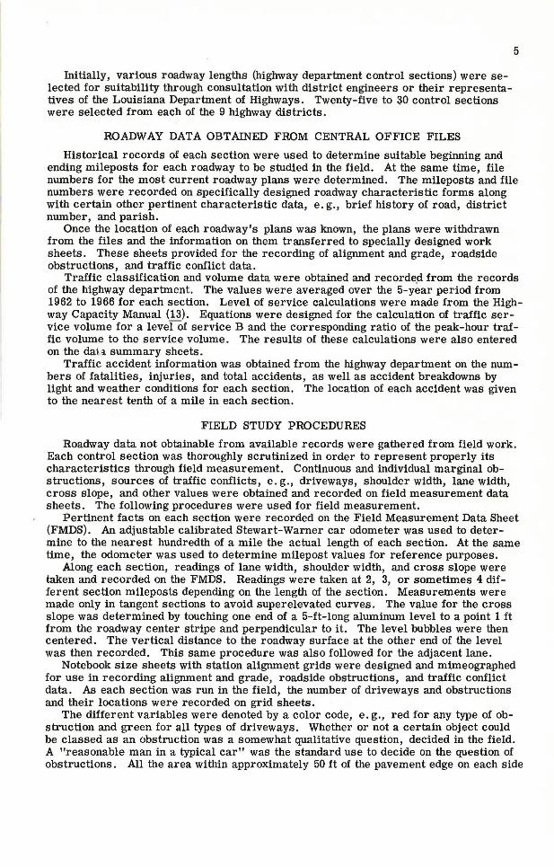
Initially, various roadway lengths (highway department control sections) were se­lected for suitability through consultation with district engineers or their representa­tives of the Louisiana Department of Highways. Twenty-five to 30 control sections were selected from each of the 9 highway districts.

ROADWAY DATA OBTAINED FROM CENTRAL OFFICE FILES

5

Historical records of each section were used to determine suitable beginning and ending mileposts for each roadway to be studied in the field. At the same time, file numbers for the most current roadway plans were determined. The mileposts and file numbers were recorded on specifically designed roadway characteristic forms along with certain other pertinent characteristic data, e.g., brief history of road, district number, and parish.

Once the location of each roadway's plans was known, the plans were withdrawn from the files and the information on them transferred to specially designed work sheets. These sheets provided for the recording of alignment and grade, roadside obstructions, and traffic conflict data.

Traffic classification and volume data were obtained and recorde.d from the records of the highway department. The values were averaged over the 5-year period from 1962 to 1966 for each section. Level of service calculations were made from the High­way Capacity Manual (13). Equations were designed for the calculation of traffic ser­vice volume for a levefOf service B and the corresponding ratio of the peak-hour traf­fic volume to the service volume. The results of these calculations were also entered on the dai a summary sheets.

Traffic accident information was obtained from the highway department on the num­bers of fatalities, injuries, and total accidents, as well as accident breakdowns by light and weather conditions for each section. The location of each accident was given to the nearest tenth of a mile in each section.

FIELD STUDY PROCEDURES

Roadway data not obtainable from available records were gathered from field work. Each control section was thoroughly scrutinized in order to represent properly its characteristics through field measurement. Continuous and individual marginal ob­structions, sources of traffic conflicts, e.g., driveways, shoulder width, lane width, cross slope, and other values were obtained and recorded on field measurement data sheets. The following procedures were used for field measurement.

Pertinent facts on each section were recorded on the Field Measurement Data Sheet (FMDS). An adjustable calibrated Stewart-Warner car odometer was used to deter­mine to the nearest hundredth of a mile the actual length of each section. At the same time, the odometer was used to determine milepost values for reference purposes.

Along each section, readings of lane width, shoulder width, and cross slope were taken and recorded on the FMDS. Readings were taken at 2, 3, or sometimes 4 dif­ferent section mileposts depending on the length of the section. Measurements were made only in tangent sections to avoid superelevated curves. The value for the cross slope was determined by touching one end of a 5-ft-long aluminum level to a point 1 ft from the roadway center stripe and perpendicular to it. The level bubbles were then centered. The vertical distance to the roadway surface at the other end of the level was then recorded. This same procedure was also followed for the adjacent lane.

Notebook size sheets with station alignment grids were designed and mimeographed for use in recording alignment and grade, roadside obstructions, and traffic conflict data. As each section was run in the field, the number of driveways and obstructions and their locations were recorded on grid sheets.

The different variables were denoted by a color code, e.g., red for any type of ob­struction and green for all types of driveways. Whether or not a certain object could be classed as an obstruction was a somewhat qualitative question, decided in the field. A "reasonable man in a typical car" was the standard use to decide on the question of obstructions. All the area within approximately 50 ft of the pavement edge on each side

6

of the road was observed. A dangerous object or continuous hazard was classed as either a continuous or a marginal obstruction if it would be encountered by a reasonably good driver in an accident situation. An example of a continuous obstruction might be a long line of trees perhaps 10 ft from the roadway or a rather steep drop".'off near the pavement edge. An example of a marginal or discrete obstruction would be a lone tree near the road.

The independent variables measured were traffic, width, cross slope, alignment, and roadside friction. The traffic variables were as follows:

1. Trucks-the percentage of the ADT that is made up of vehicles other than pas­senger cars and pickup trucks.

2. Traffic volume-24-hour, 2-way total traffic flow, commonly referred to as ADT . 3. Traffic volume ratio-the ratio of the peak hourly traffic volume (2-way) for a

highway section to its corresponding service volume for level B operation as defined by the Highway Capacity Manual (13).

The width variables were as follows:

1. Lane width-the width in feet measured between the center of a 2-lane roadway and the edge of the pavement or traveled way.

2. Shoulder width-the width in feet between the edge of the pavement or traveled way and the edge of any shoulder, generally indicated by a change in slope between the shoulder and the side slope.

The cross-slope variable is the slope of the pavement or traveled way from the center of the roadway toward the shoulder measured in feet per foot of pavement width.

The alignment variables were as follows:

1. Horizontal alignment-the percentage of the length of a highway section that has a horizontal highway curvature in excess of 3 deg.

2. Vertical alignment-the percentage of the length of a highway section that has a highway gradient in excess of 3 percent.

The roadside friction variables were as follows:

1. Continuous obstruction-the percentage of the total length of a highway section that has some roadside feature or obstacle that runs for more than a few feet on either or both sides of the roadway. Such a feature would be a deep roadside ditch or steep side slope that presents an obstacle to a vehicle's safely leaving the roadway in an emergency at posted highway speeds.

2. Marginal obstructions-the total number of discrete objects on both sides, such as a driveway embankment, culvert, roadway culvert headwall, tree, or telephone pole, per mile of a highway section within the cleared right-of-way. This is not to be confused with the marginal obstruction within 6 ft of the pavement edge used in capac­ity analysis (13).

3. Trafficconflicts-the total number of traffic access points on both sides per mile of highway section. These access points include only minor oad intersections (inter­sections with major roads were considered as break points between study sections) and principal access driveways to abutting property along highway section.

FINAL DATA PREPARATION PROCEDURES

From the summary sheets, data were transferred to code sheets for keypunching onto computer cards. Nearly all of the information previously mentioned was then re­corded on summary sheets that condensed the data for analysis. Sections were then checked for high-accident frequency values. If, after carefully studying the locations of each of these values, we found that the accidents were obviously being caused by conditions other than roadway geometry and weather conditions, we separated the ex­treme values from the sections and formed new smaller subsections, if feasible. All new summary data were then prepared on new summary forms.

7

DATA ANALYSIS PROCEDURE

Levonian (20) emphasizes that mulivariate analysis not only provides for statistical control but also retains that reliability associated with the entire sample. An impor­tant consequence is the likelihood that the prediction of accidents will be enhanced when several predictors are used. An even more important consequence of multivari­ate analysis is the clarity with which results can be interpreted; this last consequence accrues from the fact that multivariate results can be presented in an integrated rather than piecemeal fashion.

The analysis consisted first of selecting and punching the pertinent data by using a computer program to select needed data from raw data file and then a multiple regres­sion program to perform the regression analysis.

For each analysis, the independent variables used as input data and described earlier were the same. In addition to these variables, a number of indexing characteristics were used in order to segregate the data for more detailed analysis. These included the following:

1. Highway maintenance district, 8. Injury accidents, 2. Section number, 9. Total accidents, 3. Shoulder type, 10. Day accidents, 4. Traffic volume, 11. Night accidents, 5. Bridges in section, 12. Accidents on wet surface, and 6. Service volume, 13. Accidents on dry surface. 7. Fatal accidents,

The dependent variable (accidents) was grouped differently for each run. The groups, each per 100 million vehicle miles, were as follows:

1. Accidents, 5. Accidents during night, 2. Injuries, 6. Accidents on wet roads, and 3. Fatalities, 7. Accidents on dry roads. 4. Accidents during day,

It was of interest to investigate the main effects and the first order interactions {in-cluding the main effect squared terms) of the independent variables. The large number of highly significant cross products means not necessarily that one variable depends on the other but that elements of the roadway are generally built as compatible units. For example, very seldom would one suggest today that a roadway be built with a high de­gree of adequacy for surface width but a low degree of adequacy for sight distance.

SUIT ABILITY OF THE SAMPLE AND RANGE OF VALUES OBTAINED

In undertaking a project of the type and scope previously described, one needs to be particularly concerned with the adequacy of the sample to cover the full ranges of the variables involved. The following points seem appropriate as a result of this research.

1. The researchers thought that past studies attempted to analyze distributions that were too large and diverse to be meaningful in view of the scarcity of data. The sam­ple for this study included 246 sections of rural roadway, varying in length from 1 to 17 miles, on which occurred more than 6,000 accidents during the term covered by the study. Locations of the study sections are shown in Figure 1. Excellent geographical coverage of the state was obtained.

2. A primary difference between this study and others "that demonstrated a low probability of answering specific questions" lay in the fact that the researchers at­tempted to determine primarily a heirarchy of accident-cause factors. (This hierarchy might also be useful in determining optimum use of highway construction funds.) The sample of highway sections used in this study experienced over 6,000 accidents during a 5-year period. Particular care was exercised to determine that no study section had been altered during the time covered by the study. In choosing the sample sections, we took care that the entire sample provided coverage of the full range of each variable.

8

Figure 1. Location of study sections.

3. The manner in which accidents are investigated and recorded in Louisiana is entirely compatible with the requirements of the study. The accidents are reported to the nearest 0.1 mile and all the accident data required for the study were in the mem­ory oi the highway department's electronic data processing equipment. After t.lie sec­tions were selected, they were examined for a uniform distribution of accidents. Clus­tering of accidents was cause for eliminating or breaking the section up into smaller sections. No attempt was made to study only high-accident sections.

4. Every section of roadway used in this study was traveled twice for data collec­tion and surveillance purposes. If a section was not homogeneous with respect to the variables, it was either deleted or divided into 2 sections, if feasible. The terrain of Louisiana is largely rolling and hilly in the north, flat in the south. This situation helped in obtaining sections that encompassed the wide range of variables necessary for the proposed analysis. Particular attention was paid to the sections for homoge­ne~ty; that is, if a section were hilly for any part, it must be uniformly hilly through­out. If a section had few traffic access points, it must have few over the entire length of the section.

Another word about the sample. Because all data were taken in Louisiana, then the results from the satistical manipulation of the data can only apply to Louisiana. It is

reasonable to expect that causes of acci­dents may be different in each state; therefore, comparisons with other states are interesting but there should not nec­cessarily be a direct relationship.

TABLE 2

VALUE RANGES FOR INDEPENDENT VARIABLES

Variable

Traffic Trucks

Value Range

2 to 33 percent of traffic

9

The ranges of values for each of the independent variables studied on the 246 study sections are given in Table 2.

Traffic volume Traffic volume ratio

190 to 11,933 vehicles per day 0.04 to 2.12

INDIVIDUAL VARIABLE RELATION­SHIPS TO ACCIDENT RATE

Each independent variable was plotted against total accident rate (accidents per million vehicle miles) to see what trends existed. Some of these relationships are shown in Figures 2 through 5. In each case the curves represent general trends of the raw data available.

Of particular interest are those that can be compared with previously reported studies. Figure 2 shows a trend typical

Width Lane width Shoulder width

Cross slope

Alignment Horizontal alignment

Vertical alignment

Roadside friction Continuous obstructions

Marginal obstructions Traffic conflicts

9 to 12 ft 1 to 12 ft

0,000 to 0.038 It/ft

0 to 57 . 5 percent of length > 3 deg

0 to 48.0 percent of length > 3 percent

0 to 100 percent of section length

0 to 34 per mile 0 to 46 per mile

of many previous studies (35, Ch. II) in which accident rates increase as traffic flow increases. More specifically, the curve shown in Figure 2 compares well with that in Rykken's Figure 6 (35) where a congestion index is used similar to the traffic volume ratio used here. The data shown in Figure 3 permit a direct comparison with those ob­tained by Charlesworth (34). The general aggreement of the data in Figures 2 and 3 with those previously reported by others indicates that the data obtained in this research are representative and quite usable for the intended purposes.

Of particular interest are· the comparisons of accident rate with the 2 most important in­dependent variables as shown by regression analyses. Figure 4 shows a very solid straight-

2.•

2.•

(/)

(/) w _, 2.2

~ ~L.S.U , DATA

~ ~ w 2.2

u w ..... u J: w 2.0 > J:

w z ~ENGLISH DATA

(After Charlesworth, Ref. 3.4, p. 16)

> z 2.0

0 ::::; ..... ~

"' 1.B

w c.. (/) 0 I-z LU 1.6 Q u u <

'·' 0

0.2 0. 06 o.e 1,0

TRAFFIC VOLUME RATIO

(PEAK HOUR VOLUME/ SERVICE VOLUME AT LEVEL B)

Figure 2. Accident rate versus traffic volume ratio.

1 2

0 ::::; _, 1.8

~

"' w c.. Vl 1-z w 0 u u <

1.6

1-2 ___ ..____ _ ____.,..._ __ __,_ _ _ ....... _

10 11 12

LANE WIDTH, FT.

Figure 3. Accident rate versus lane width.

10

"' w ..... i ~ u :I: w > z 0 :::; ..... i "' w 0..

"' >-z w c u u <

2. 2.0

0 "' ~ 2. 2

i ~ 1.8

!::! :I: w > 2 0 z 1.6 0 0 :::; .....

~ 1. 8 i 0

"' u

w 0..

"' 0 >-1.6 z

w 1.2 0 c 0 u u

< 0 1.4 0

1.0 0 0 0.005 0010 0 015 0.020 0 015

0 CROSS SLOPE, FT./FT. 1.2

Figure 5. Accident rate versus pavement cross slope. 1 0

12 16 20

TRAFFIC CONFLICTS PER MILE

line trend of accident rate increasing with Figure 4. Accident rate versus traffic conflicts. an increase of traffic conflict points per

mile. This trend also correlates well with previously reported research, especially that of Mulinazzi and Michael (27). Fig­ure 5, on the other hand, showsa rela-

tionship not previously reported and one that definitely indicates that r oadways with relatively flat cros s s lopes are more accident prone than those with better slopes .

REGRESSION ANALYSES

The primary purpose of this study was to define those geometric characteristics of the roadway that were most responsible for accidents.

Total Accidents Analysis

The analysis of all 246 sections with respect to total accidents yielded the following hierarchy of importance (all first order interactions):

1. Traffic volunie and pavement cross slope, 2. Traffic conflicts and traffic volume, 3. Lane width and traffic conflicts, 4. Traffic volume and horizontal alignment, 5. Shoulder width and horizontal alignment, and 6. Traffic volume and trucks.

The effects of traffic volumes, traffic conflicts, horizontal alignment, lane widths, and shoulder widths have been cited in previous research. However, it is important to note the hierarchy of their effects in the Louisiana evironment. Of particular inter ­est in this analysis is the r elative importance of cross s lope. This is of particular significance in areas such as Louisiana because of the high rainfall (60 in. per year near Baton Rouge) that may lead to hydroplaning effects in the presence of low cross­slope values.

11

Other Analyses

The regression analyses of !;tll sections with respect to accidents classed as injury, fatalities, wet surface, dry surface, day, and night yielded some differences in the hierarchy of variables. Table 3 gives the results of 8 regression analyses including both total accident analyses (all variables versus main effects only). Only the top 4 variables are given because they had the highest F-values for being entered into the regression analysis and also generally contributed to no less than about 1 percent of the cumulative R 2 value.

In all analyses it is significant that the one variable that contributed most to the ac­cident rate was the traffic volume ratio. This indicates that the more nearly a road­way carries traffic volumes approaching or greater than its design service volume, the

TABLE 3

FOUR VARIABLES CONTRIBUTING MOST TO MULTIPLE R 2 VALUES

Accidents Analyzed Variables Variable Multiple Order R'

Total accidents: all first order variables versus main effects

First order TVR x CS l 0.305 TVR x TC 2 0.365 LW x TC 3 0.386 TVR x HA 4 0.398 All 0.587

Main effects TVR l 0.241 cs 2 0.265 VA 3 0.272 TC 1 0.278 Ten 0.295

Fatalities versus injuries

Fatalities TVR x CS 1 0.136 CS x TC 2 0.179 HA x VA 3 0.199 SW x CO 4 0.209 All 0,424

Injuries TVR x CS 1 0.304 TVR x TC 2 0.358 LW xTC 3 0.388 TVR x HA 4 0.404 All 0.610

Day versus night

Day TVR x CS 1 0.307 TVR x TC 2 0.354 T x TVR 3 0.374 TVR x HA 4 0.384 All 0.588

Night (TVR)' 1 0.258 TVR x TC 2 0.300 TVR x CS 3 0.327 LW xTC 4 0,347 All 0.537

Dry versus wet road

Dry (TVR) 2 1 0.303 TVR x TC 2 0.352 TVR x CS 3 0.378 TVR 4 0.402 All 0.615

Wet TVR x CS 1 0.291 T x TVR 2 0.331 (T)2 3 0,337 TVR 4 0,352 All 0.487

Note: cs cross slope co continuous obstructions TC traffic conflicts HA horizontal alignment T trucks TVR traffic volume ratio LW lane width SW shoulder width VA vertical alignment

12

more likely it will experience a greater accident rate. The analyses also show that the most important geometric features affecting accident rates are pavement cross slope and traffic conflicts per mile.

Mathematical Model

Although mathematical models were prepared for all 7 analyses, the authors con­sider the analysis for total accidents to be the most important one. The mathematical model for this analysis is given in the Appendix.

In statistical terms, the product of correlation, XlOO, is defined as "the percent of variation in the data that is accounted for by the mathematical formula." Accordingly, the product of correlation, R 2

, value obtained for the total accident model was 0.46, which indicates that the model explains 46 percent of the variation in the data. What does this really say? It says the 46 percent of the variation in the data is explained by the geometric factors that were included in the study. The remaining 54 percent is accounted for by variables not included in this study. Those are probably driver, environmental, and vehicle variables as well as other roadway variables not included and various interactions of all variables. The approximately 46 percent of the varia­tion is in line with what authorities such as Baldwin (2) have suggested. In 1942 ~m~(37)s~: -

The roadway may contribute directly to accidents, or an accident may result from a number of causes one of which may be traced to an inherent deficiency in the road. Accidents which are directly caused by "defects" in the roadway are believed to number from 3 to 10 percent of all accidents. If we include all accidents in which a "fault" may have been one of the contribut­ing causes it is conceivable that 15 to 40 percent of accidents may be traceable directly or in­directly to the road .

More important than the model itself is its application and use as a possible tool for determining the probable accident rate for a proposed highway design . An example of the use of this model is given in the .Appendix.

CONCLUSIONS

A criticism of the type of study undertaken here is that one obtains a lot of informa­tion that is intuitively obvious. That is, everyone knows that hills, curves, and a great deal of traffic will indicate high-accident experiences. This, of course, is true, and the fact that many of these factors do indeed come to the front comforts the researcher that his methodology is correct. How much do each of these factors contribute? This study has quantified the answer to this question. What about the occasional surprises? For instance, the relative importance of horizontal alignment over vertical alignment seems significant. The relative importance of cross slope seems to indicate that fur­ther study in this direction might prove fruitful. So the occasional surprises probably will more than justify the effort of the study.

This study is all-inclusive so that, of necessity, later studies must be concerned with specific design features that are here shown to be of importance.

Based on multiple regression analyses of data for Louisiana rural highways only, the following conclusions seem valid relating accidents to highway geometry:

1. Only 46 percent of the variation in accident rates is explained by the geometric factors that were included in U1is study. This indicates that 54 percent of the variation in accidents was caused by the driver, the vehicle, or by other variables that were not included in this study.

2. The methodology used and the results obtained appear to be valid based on limited comparisons with results of previously conducted research.

3. The 2 geometric variables appearing to have the most important effect on acci­dent rates, based on their interactions with traffic volume, are pavement cross slope and the number of traffic conflicts per mile.

13

4. Of the geometric variables investigated, continuous obstructions, marginal ob­structions, and their interaction terms had the least effect on accidents. This indicates that the variation in accidents was least caused by obstructions off of the right-of-way.

5. The project has been successful in relating several geometric variables to acci­dent rates and has produced the following hierarchy of importance, all first-level interactions: traffic volume and pavement cross slope, traffic conflicts and traffic volume, lane width and traffic conflicts, traffic volume and horizontal alignment, shoulder width and horizontal alignment, and traffic volume and percentage of trucks.

6. A mathematical model has been developed that will help predict the accident picture likely to be experienced on a roadway, given the characteristics of that road­way.

RECOMMENDATIONS

Based on the results of this project, recommendations are as follows:

1. That the utilization of the mathematical models derived from this research be considered to determine how to allocate funds for highway accident reduction;

2. That particular attention be focused on the geometric variables of traffic con­flicts and pavement cross slope in any highway improvement project;

3. That additional research be considered to investigate further the effect of pave­ment cross slope on vehicle performance and accident rate ; and

4. That additional research be considered to ascertain ways to reduce accidents resulting from sources of traffic conflicts.

REFERENCES

1. A Policy on Geometric Design of Rural Highways. American Association of State Highway Officials, 1966.

2. Baldwin, D. M. The Relation of Highway Design to Traffic Accident Experience. American Association of State Highway Officials Convention Group Meetings, 1946, pp. 103-109.

3. Belmont, D. M. Accidents Versus the Width of Paved Shoulders on California Two-Lane Tangents-1951-1952. HRB Bull. 117, 1956, pp. 1-16.

4. Bitzl, F. Accidents Rates on German Expressways in Relation to Traffic Vol­umes and Geometric Design. Roads and Road Construction, Jan. 1957, pp. 18-20.

5. Blensly, R. C ., and Head, J. A. Statistical Determination of Effect of Paved Shoulder Width on Traffic Accident Frequency. HRB Bull. 240, 1960, pp. 1-23.

6. Boodman, D. M. What We Know and Don't Know About Traffic Safety. Arthur D. Little, Inc., Cambridge, Mass., 1967.

7. Cirillo, J. A. Interstate System Accident Research-Study II. Highway Research Record 188, 1967, pp. 1-7.

8. Claes, M. G. A Study of Accident Rates in Belgium. futernational Course in Traffic Engineering Reports, Theme III, 1954.

9. Cribbins, P. 0., et al. The Effects of Selected Roadway and Operational Char­acteristics Upon Accidents on Multilane Highways. Highway Research Record 188, 1967, pp. 8-25.

10. Crosby, J. R. Cross-Median Accident Experience on the New Jersey Turnpike. HRB Bull. 266, 1960, pp. 63-77.

11. Dunlap, J. W., Orlansky, J., and Jacobs, H. H. Manual for the Application of Statistical Techniques for Use in Accident Control. U.S. Dept. of Commerce, Office of Technical Services, June 1958.

12. Haddon, W., Jr., Suchman, E. A., and Klein, D . .Accident Research. Harper and Row, 1964.

13. Highway Capacity Manual-1965. HRB Spec. Rept. 87, 1965. 14. Hiller, J. A., and Wardrop, J. G. Effect of Gradient and Curvature on Accidents

on London-Birmingham Motorway. Traffic Engineering and Control, Vol. 7, No. 10, Feb. 1966, pp. 617-621.

14

15. Iowa Reports on Traffic Accidents. American Highways, Vol. 41, No. 4, Oct. 1962, pp. 22-24.

16. Guidelines for .Accident Reduction Through Programming of Highway Safety Im­provements. Roy Jorgensen and Associates, Gaithersburg, Md., a report to the U.S. Bureau of Public Roads, Dec. 1964.

17. Evaluation of Criteria for Safety Improvements on the Highway. Roy Jorgensen and Associates, Gaithersburg, Md., 1966.

18. Killlberg, . K., and Tharp, K . J. .Accident Rates as Related to Design Elements of Rural Highways. NCHRP Rept. 47, 1968.

19. Lacy, J. D. Highway Safety Improvement Projects-Evaluation of Improvements. U.S. Bureau of Public Roads, Circular Mem orandum, April 1, 1966.

20. Levonian, E., Case, H. W., and Gregory, R. Prediction of Recorded Accidents and Violations Using Nondriving Predictors. Highway Research Record 4, 1963, pp. 50-61.

21. McCormack, C. F. A Plan for Relating Traffic Accidents to Highway Elements. American Association of State Highway Officials Convention Group Meeting, 1944, pp. 117-119.

22. Michaels, R. M. Two Simple Techniques for Determining the Significance of Accident-Reducing Measures. Traffic Engineering, Vol. 36, No. 12, Sept. 1966, pp. 45-48.

23. Miller, H. G. Safety Holds the Line in 1967. Traffic Safety, Vol. 68, No. 3, March 1968, pp. 12- 14, 30- 31.

24. Morin, D. A. Application of Statistical Concepts of Accident Data. Highway Research Record 188, 1967, pp. 72-79.

25. Mosher, W.W., Jr. Traffic Safety and the New Technology. American Engi­neer, July 1966, p. 27.

26. Moskowitz, K., and Schaefer, W. E. California Median Study: 1958. HRB Bull. 266, 1960, pp. 34-62.

27. Mulinazzi, T. E., and Michael, H. L. Correlation of Design Characteristics and Operational Controls with Accident RaJes on Urban Arterials. Purdue Univ., Lafayette, Ind., Joint Highway Research Project Rept. 35, Dec. 1967.

28. Norden, M. L., Orlansky, J., and Jacobs, IL H. Application of Statistical Quality-Control Techniques to Analysis of Highway-Accident Data. HRB Bull. 117, 1956, pp. 17- 31.

29. Perkins, E. T. Relationship of Accident Rate to Highway Shoulder Width. HRB Bull. 151, 1957, pp. 13- 14.

30. Raff, M. S. Interstate Highway-Accident Study. HRB Bull. 74, 1953, pp. 18-45. 31. Schoppert, D. W. Predicting Traffic Accidents From Roadway Elements of Rural

Two-Lane Highways With Gravel Shoulders. HRB Bull. 158, 1957, pp. 4-26. 32 . Sparks, J. W. The Influence of Highway Characteristics on Accident Rates.

Public Works, Vol. 99, No. 3, March 1968, pp. 101-103, 120. 33. Stohner, W. A. Relation of Highway Accidents to Shoulder Width on Two-Lane

Rural Highways in New York State. HRB Proc., Vol. 35, 1956, pp. 500-504 . 34. Stonex, K. A. Roadside Design for Safety. HRB Proc., Vol. 39, 1960, pp. 120-

156. 35. Traffic Control and Roadway Elements-Their Relationship to Highway Safety.

Automative Safety Foundation and U.S. Bureau of Public Roads, 1963. 36. Whitton, R. M. The Systems Approach to Traffic Safety. Civil Engineering,

Vol. 36, No. 9, Sepl. 1966, pp. 40-42. 37. De Silva, H. R. Why We Have Automobile Accidents. John Wiley and Sons, New

York, 1942, p. 269.

Appendix

MATHEMATICAL MODEL

The following is the model for total accidents per 100 million vehicle miles. The R2 is 0.46 and all of the F-ratios are significant at the 0.05 level.

y 41.32 - 1.23X1 - 0.54X2 - 0.67X6 + 0.03X1X2 + 0.03X:?'6 - 0.0009X~9

+ 0.026X~11 - 0.12X4X11 + 0.009X5X9

where

total accidents per 100 million vehicle miles, percentage of trucks, traffic volume ratio, cross slope, (percentage of trucks) (traffic volume ratio),

= (traffic volume ratio) (cross slope), = (traffic volume ratio) (horizontal alignment), = (traffic volume ratio) (traffic conflicts),

(lane width) (traffic conflicts) , and = (shoulder width) (horizontal alignment).

15

The mathematical models can be used to predict the number of accidents per 100 million vehicle miles, given the various geometric characteristics (independent vari­ables) included in the model. The model for total accidents is used in this example.

The calculated value for the accident ratio can be obtained by using the equation for y in the mathematical model and substituting numbers in the correct units for the var­ious X's. Average values were selected for the independent variables and were coded to be compatible with the computer program. They are as follows (their more famil­iar forms are in parentheses):

X1 percentage of trucks = 13, X2 traffic = 55 (0.55), X4 lane width = 11, Xs shoulder width = 8, X6 cross slope = 12.8 (0.0128 ft/ft), X 7 percentage of continuous obstructions = 66, X8 marginal obstructions per mile = 7. 5, X 9 horizontal alignment = 57 (57 percent of section ::> 3 deg),

X 10 vertical alignment = 50 (50 percent of section ::> 3 percent), and X11 traffic access points per mile = 9.

When these values are substituted in the equation for total accidents per 100 million vehicle miles, the following is obtained:

y = 28.65 accidents per 100 million vehicle miles

With a given confidence value, the range of y can be determined. This equation is

y' = y ±ta, N Sy

where

Y' range of y, ta N distribution that is a function of a and N,

' a confidence limits, N degrees of freedom, and

Sy standard deviation of y.

16

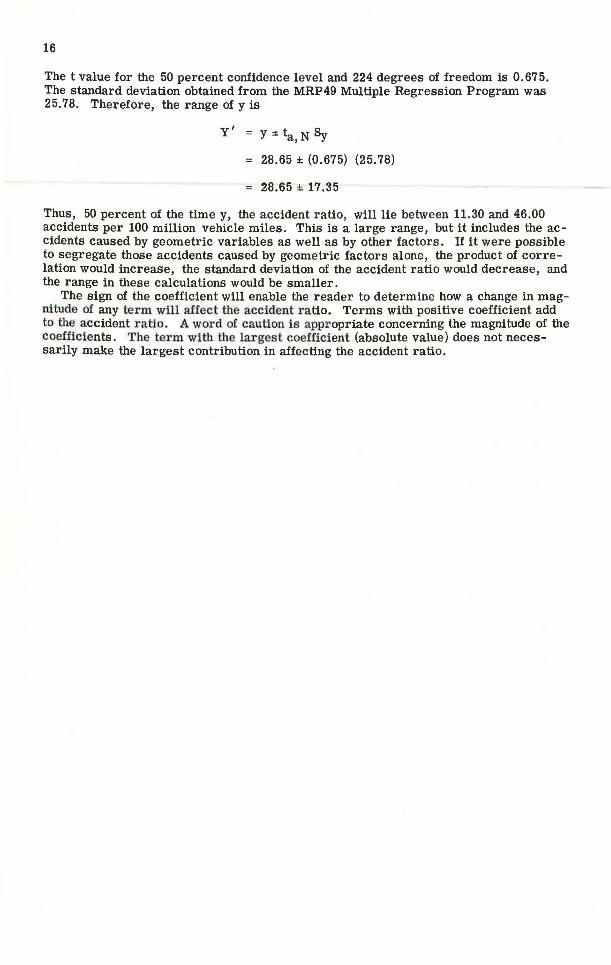
The t value for the 50 percent confidence level and 224 degrees of freedom is 0.675. The standard deviation obtained from the MRP49 Multiple Regression Program was 25.78. Therefore, the range of y is

y' y ±ta, N Sy

28.65 ± (0.675} (25.78)

28.65 ± 17.35

Thus, 50 percent of the time y, the accident ratio, will lie between 11.30 and 46.00 accidents per 100 million vehicle miles. This is a large range, but it includes the ac­cidents caused by geometric variables as well as by other factors . If it were possible to segregate those accidents caused by geometric factors alone, the product of corre­lation would increase, the standard deviation of the accident ratio would decrease, and the range in these calculations would be smaller.

The sign of the coefficient will enable the reader to determine how a change in mag­nHude of any te rm will affect the accident ratio. Terms with positive coefficient add to the accident ratio. A word of caution is appropriate concerning the magnitude of the coefficients. The ter m with the larges t coefficient (absolute value) does not neces­sarily make the largest contribution in affecting the accident ratio.