Highly charged cloud particles in the atmosphere of Venushome.iitk.ac.in/~snt/pdf/Michael_VenusCloudCharging.pdf · Highly charged cloud particles in the atmosphere of Venus ... W

Highly charged cloud particles in the atmosphere of Venus

Marykutty Michael,1 Sachchida Nand Tripathi,1 W. J. Borucki,2 and R. C. Whitten3

Received 12 September 2008; revised 25 December 2008; accepted 21 January 2009; published 17 April 2009.

[1] The accumulation of charges on cloud particles by the charge transfer of ions andattachment of electrons in the atmosphere of Venus is investigated in the present work.Three cloud layers between 45 and 70 km exist in the atmosphere of Venus. Ions andelectrons are produced by the interaction of galactic cosmic rays with the neutralmolecules. Ion to particle and electron to particle attachment coefficients are calculated.The charge balance equations include ion-ion recombination, ion-electron recombination,electron attachment to neutrals, electron detachment from negative ions, and attachment ofelectron and charge transfer from ions to particles. It is found that the ion concentrationsare reduced by a maximum of a factor of 5 by charging of the particles, while the earlierstudies showed a maximum reduction of about an order of magnitude due to thedifferences in the surface area of the particles. A similar result is observed in thecalculation of electrical conductivity. Both monodisperse and polydisperse distribution ofparticles are considered. The conductivity was reduced by a factor of 3 when using themonodisperse distribution of particles, while the maximum reduction observed was afactor of 2 when using the polydisperse distribution. This result implies that themonodisperse particle distribution overestimates the effect of particles on the atmosphericconductivity. The ratio of negative to positive charges is found to be very large in themiddle and upper cloud layers. The low abundance of the aerosols and high conductivityof the atmosphere appear to rule out lightning activity in the 40 to 70 km altitude region.

Citation: Michael, M., S. N. Tripathi, W. J. Borucki, and R. C. Whitten (2009), Highly charged cloud particles in the atmosphere of

Venus, J. Geophys. Res., 114, E04008, doi:10.1029/2008JE003258.

1. Introduction

[2] Mariner 10 and Pioneer Venus measurements revealedwidespread hazes in the atmosphere of Venus. Generallythey cover the entire planet, being most prominent at thebright polar caps [Taylor et al., 1980; Knollenberg andHunten, 1980; Turco et al., 1983]. Haze is considered as anaerosol that impedes vision and may consists of droplets,and dust usually of size less than 1 mm. The clouds aregenerally thought of as a photochemical haze observed inthe altitude range of 45–70 km. In situ probe measurementsdetected three cloud layers (upper, middle, and lower) basedon distinctive cloud particle size distributions of �0.4, �2and �7 mm [Esposito et al., 1983; Crisp et al., 1991;Carlson et al., 1993; Grinspoon et al., 1993]. The thickopaque cloud region between 48 and 56 km has beenobserved on Galileo and ground-based near-infrared imagesof Venus [Crisp et al., 1989; Bell et al., 1991; Carlson et al.,1993; Grinspoon et al., 1993]. Microphysical processes inthe cloud layer are described in detail in various papers[e.g., Toon et al., 1982; James et al., 1997; Imamura andHashimoto, 1998, 2001]. Two different mechanisms have

been invoked to explain the formation of these clouds. Nearthe cloud top, photochemistry leads to the formation ofcloud particles [Krasnopolsky and Pollack, 1994; Mills andAllen, 2007]; near the cloud base, condensation of sulfuricacid vapor on hydrated sulfuric acid particles may be respon-sible for the particle formation [Young, 1973; Rossow, 1978].According to Aplin [2006], the sulfuric acid condensationonto ions also plays a role in the formation of cloud particlesin 42–44 km region in the atmosphere. The cloud particleshave a number density ranging from 100 to 1000 cm�3 andthe particle size distribution is bimodal [Knollenberg andHunten, 1980; Pollack et al., 1993; Grinspoon et al., 1993;Krasnopolsky, 1989]. An upper haze layer is observed in thealtitude range of 70 to 90 km, containing particles with aneffective radius of 0.2–0.3 mm, composed of H2SO4/H2Oaerosol with 75% sulfuric acid [Kawabata et al., 1980]. Atransport model between this haze layer and the atmosphericcloud is discussed by Yamamoto and Takahashi [2006]. TheVenus Monitoring Camera (VMC) onboard Venus Expressspacecraft investigated the global and small-scale propertiesof the upper cloud layer of Venus and found that the polarcloud pattern was highly variable on short time scales[Markiewicz et al., 2007]. VMC also found that the polarhaze expanded to the mid latitudes and the equatorial cloudshowed wavy and streaky morphology [Markiewicz et al.,2007]. The abundance and size distributions of the cloud andhaze layers are shown in Figure 1.

JOURNAL OF GEOPHYSICAL RESEARCH, VOL. 114, E04008, doi:10.1029/2008JE003258, 2009ClickHere

for

FullArticle

1Department of Civil Engineering, Indian Institute of Technology,Kanpur, India.

2NASA Ames Research Center, Moffett Field, California, USA.3SETI Research Institute, Mountain View, California, USA.

Copyright 2009 by the American Geophysical Union.0148-0227/09/2008JE003258$09.00

E04008 1 of 18

http://dx.doi.org/10.1029/2008JE003258

[3] The cloud particles are charged by the attachment ofelectrons to the particles and charge transfer from the ions.Attachment and charge transfer to particles is a loss mech-anism for electrons and ions and causes a reduction inatmospheric electrical conductivity. Since the cloud cover isubiquitous in the atmosphere of Venus, reduced conductiv-ity is a global phenomenon. Borucki et al. [1982] have

calculated the conductivity of the lower atmosphere ofVenus, taking into account the then available data on theatmospheric environment and the cloud particles. Theirstudy showed that the great abundance of cloud particlescaused significant reductions of the conductivity within theclouds and has implications for lightning activity [Boruckiet al., 1982; Russell, 1991].

Figure 1. (a) Altitude profile of the size-integrated distribution and (b) effective particle radii [James etal., 1997] along with the cloud layers. (c) Concentration and (d) radius of monodisperse cloud particlesused in the present work are compared with those used by Borucki et al. [1982].

E04008 MICHAEL ET AL.: CLOUD CHARGING IN VENUS

2 of 18

E04008

[4] Lightning is a large-scale electric discharge thatoccurs in the planetary atmospheres when the electric fieldreaches a critical value. In the Earth’s atmosphere, lightningis produced by thunderclouds and most of the dischargesoccur within the clouds. Most discharges begin within thecloud where there are large concentrations of positive andnegative space charge. Electrification intensifies as theconvective activity increases, and becomes intense whenthere is rapid vertical growth of the cloud with the devel-opment of precipitation. Though the searches for the exis-tence of lightning in Venus in the past have been bothpositive [Krasnopolsky, 1983; Gurnett et al., 1991; Hansellet al., 1995] and negative [Sagdeev et al., 1986; Borucki etal., 1991; Gurnett et al., 2001], the recent observations bythe Venus Express instruments detected strong, circularlypolarized electromagnetic waves which have the expectedproperties of signals generated by lightning discharges[Russell et al., 2007]. In the middle cloud layer, thetemperature and pressure are almost Earth-like with apressure close to 0.5 bar and a temperature of about315 K. The clouds are thought to be composed of H2SO4

droplets, which are readily charged. Thus, lightning couldoccur if convection produces large potential differenceswithin the clouds. Russell et al. [2007] also inferred that,in the Venusian atmosphere most discharges consist ofintracloud strokes. The presence of lightning on Venusimplies the existence of atmospheric regions in whichcharge separation mechanisms operate at a rate sufficientto overcome the dissipation of the separated charge byatmospheric conduction [Borucki et al., 1982]. Atmosphericelectrification at various bodies in the solar system has beenreviewed by Desch et al. [2002] and Aplin [2006]. Thereview of Yair et al. [2008] suggested that there is a lack ofmodeling work to understand the charging of cloud particlesand the production of lightning discharges.[5] In this work, the influence of cloud particles on the

conductivity profile of the lower atmosphere between 40 to70 km is studied. The thin haze layer that exists above 70 kmis too tenuous, and Borucki et al. [1982] calculated thereduction in atmospheric conductivity due to the presence ofthis haze to be not very significant (<15%).[6] In order to study the conductivity of the atmosphere,

it is necessary to understand the ion production rates,composition, concentration, mobility, attachment coeffi-cients to particles, and concentration and size distributionof particles. The input data, the numerical method tocalculate the steady state concentration of ions, electronsand cloud particles, and the results are discussed in thefollowing sections. The present work uses more recent dataon the atmospheric environment and particle characteristicsthan those used by Borucki et al. [1982]. A more efficientmethod is used in the present work to calculate the ion andelectron charge transfer and attachment coefficients toparticles. The present model considers a polydisperse dis-tribution of particles, whereas Borucki et al. [1982] usedone, two, or three monodisperse distributions varying withaltitude. A Runge-Kutta method is used in the present studywhich is different than the numerical method used byBorucki et al. [1982]. All the differences and similaritiesof the input parameters and the results are compared withthose of Borucki et al. [1982]. The implication of large

charges on the cloud particles for lightning in the atmo-sphere of Venus is also discussed.

2. Ion Production

[7] Chen and Nagy [1978] have shown that the ionizingsolar ultraviolet radiation does not penetrate much below�120 km. Thus, below �70 km (the region of interest of thepresent study) galactic cosmic rays (GCR) are the principalionizing agent for the atmosphere. The incident radiation ismainly atomic nuclei, consisting of �90% protons, �10%He nuclei, and about l% heavier nuclei [Upadhyay et al.,1994].[8] The shape of the cosmic ray spectrum is such that a

significant fraction of the total energy flux is carried byparticles with kinetic energies above 1 GeV. Borucki et al.[1982] used the method developed by O’Brien [1970] tocalculate the cosmic ray–induced ionization rates in theVenusian atmosphere. Ionization of the atmosphere byenergetic particles produces primary ions CO2

+, CO+, andO2+ and electrons. Because the collision frequency with

neutral species is large, the primary ions and electronsrapidly form secondary ions and ion clusters. The conduc-tivity of the atmosphere is governed by the mobility of theselong-lived secondary ions and ion clusters, rather than bythe very mobile, but short-lived, primary ions and electrons.Borucki et al. [1982] estimated that ions such as H3O

+.SO2

(81 amu), H3O+H2O.CO2 (81 amu), H3O

+.(H2O)3 (73 amu),and H3O

+.(H2O)4 (91 amu) are the most abundant positiveion clusters and that these dominate the conductivity owingto positive ions. In the atmosphere of Venus, sulfur dioxideand oxygen are the major gaseous species to which freeelectrons may attach. O2

� readily transfers its charge tosulfur dioxide and the subsequent reactions of SO2

� areuncertain. The study of Keesee et al. [1980] suggested that(SO2)2

� would prevail above about 25 km. A review of thecluster ions produced, their interaction with the particles andthe atmospheric electrification is reported by Aplin [2006].The ion production rates reported by Borucki et al. [1982],which has been considered the best estimate [Aplin, 2006],have been used in the present work for altitudes less than70 km in the Venusian atmosphere; the mass of positive andnegative ions clusters considered are 83 and 128 amu,respectively.

3. Venusian Clouds

[9] The clouds of Venus are generally thought of as aphotochemical haze observed in the altitude range of 45–70 km. Droplets of H2SO4 + H2O were identified in theupper cloud layer from polarimetric observations [Hansenand Hovenier, 1974] who suggested an H2SO4 concentra-tion of �75 wt %. Spectroscopic observations by Pollack etal. [1978] showed that the concentration of H2SO4 is �84 ±2 wt % at the cloud tops, and the consistency of thisconcentration level with gaseous concentrations in the cloudtop region has been emphasized recently by Krasnopolsky[2007]. The modeling study by Krasnopolsky and Pollack[1994] suggested that the H2SO4–H2O system in the Venusclouds has a constant H2SO4 concentration of 85 wt % forthe sulfuric acid aerosols in the upper cloud layer, increas-ing to 98 wt % at the lower cloud boundary. Microphysical


3 of 18

E04008

processes in the cloud layer are described in detail invarious papers [e.g., Toon et al., 1982; James et al., 1997;Imamura and Hashimoto, 1998, 2001].[10] James et al. [1997] developed a numerical micro-

physical model of the condensational cloud of Venus, whichtreats vertical transport of sulfuric acid and water solutionaerosols, their nucleation, growth, evaporation, coagulation,and sedimentation. The vertical profiles of sulfuric acid gasand water vapor, cloud microphysical properties and theacid concentration of the aerosol particles are predicted bythe model of James et al. [1997] and are in agreementwith Pioneer Venus observational data and Magellan radiooccultation data. They found that the lower Venus cloud isformed as a consequence of a large upward flux of sulfuricacid vapor from the evaporation region below the cloudbase and that the heterogeneous nucleation of sulfuric acidand water vapors is a plausible mechanism for the forma-tion of the lower cloud in the atmosphere of Venus. Thesize distribution of cloud particles is approximately bi-modal in the middle cloud and trimodal in the lower cloud.The smallest mode is formed by cloud condensation nucleidiffused from below the cloud. The largest mode is formedby cloud droplets nucleated near the top of the cloud. Thedroplets continue to grow while sedimenting; thus, the

mean size of this mode increases toward the bottom of thecloud. The middle mode, present in the lower cloud, is aresult of heterogeneous nucleation on soluble cores. Theaerosols that contain enough soluble material to reduce thevapor pressure significantly are activated to become clouddroplets and form this mode. Those containing less solublematerial remain behind as aerosols of the smallest mode[James et al., 1997].[11] In the present work, the lower cloud region is

considered to be the altitude region from 40 to 48 km, themiddle cloud as the altitude region 49 to 52 km, and theupper cloud as the altitude region from 53 to 70 km. Aschematic of the cloud layers is presented in Figures 1a and1b. The lower cloud layer is considered to have a trimodaldistribution of particles while the middle and upper layersare considered bimodal. James et al. [1997] reported thelognormal distribution of cloud particles at various altitudescorresponding to the lower, middle, and upper cloud layers.These distributions are used in the present work for thealtitudes considered in the model corresponding to thelower, middle, and upper cloud layers. The effective radiiof particles (0.02 to 10 mm) are divided into 10 bins in ageometric progression. The abundance and size distributionof particles which are observed by the Pioneer Venus

Figure 2. Polydisperse distribution of cloud particles at various altitudes.

Table 1. Properties of Polydisperse Distribution of Cloud Particlesa

Mode 1 Mode 2 Mode 3

rm (mm) s rm (mm) s rm (mm) s

Lower cloud (40–48 km) 0.10 1.20 0.25 1.23 4.00 1.80Middle cloud (49–52 km) 0.15 1.25 3.50 1.90 - -Upper cloud (53–70 km) 0.18 1.29 1.00 2.16 - -

aMode 1, mode 2, and mode 3 are lognormal distributions, N(r) = (N/(ffiffiffiffiffiffi2p

pr ln s)) exp [�(ln r � ln rm)

2/(2ln2 s)]. The mean radius is rm, and thestandard deviation is s.


4 of 18

E04008

instruments [Knollenberg and Hunten, 1980] are modeledby James et al. [1997] and are used in the present study (seeFigures 1a and 1b, respectively). The particle concentrationand effective radii used by Borucki et al. [1982] arecompared with those used in the present work and arepresented in Figures 1c and 1d, respectively. The polydis-perse distribution generated is presented in Figure 2, and theparameters are presented in Table 1. This distribution is

superior to those three monodisperse distributions of par-ticles used by Borucki et al. [1982], where the radii remainalmost a constant for each distribution.

4. Description of the Model and Methodof Calculation

[12] The flow diagram of the model for the charging ofparticles by the attachment of ions and electrons is pre-sented in Figure 3. The basic inputs to the model are thestandard atmosphere (temperature and pressure), aerosolabundance, and effective radii of aerosols. The aerosolabundance and the effective radii were discussed insection 3. The production of ions and electrons by theinteraction of GCR was discussed in section 2. The neutralnumber density and temperature profiles are taken fromKrasnopolsky [2007] and Bertaux et al. [2007] and areprovided in Figures 4 and 5. The neutral number densityand temperature are similar to those used by Borucki et al.[1982] as shown in Figures 4 and 5. The ion mobility andthe ion mean free path agree very well with those used byBorucki et al. [1982]. The ion-ion recombination coeffi-cient is calculated using the method of Hua and Holzworth[1996] and is within 20% of that used in the work ofBorucki et al. [1982] for regions where clouds are present(40 to 70 km). Tinsley and Zhou [2006] used a differentexpression to calculate the ion-ion recombination coeffi-cient and found to be in the same order of magnitude asused in the present study and using their expression doesnot alter the atmospheric conductivity significantly (<10%).The electron-ion recombination coefficient and the electron

Figure 4. Neutral concentration of the atmosphere of Venus used in the present study compared withthat used by Borucki et al. [1982].

Figure 3. Flow diagram of the charging calculation ofaerosols in the atmosphere of Venus.


5 of 18

E04008

detachment coefficients are similar to those calculated byBorucki et al. [1982]. The ion charge transfer and electronattachment coefficients are calculated using the method de-veloped by Hoppel and Frick [1986]. This calculation isdiscussed byMichael et al. [2007, 2008],Tripathi andMichael

[2008], and Tripathi et al. [2008]. The typical values of thesecoefficients of positive ions, negative ions and electrons at55 km in the atmosphere of Venus are provided inFigures 6a–6c, respectively and those at 49 km arepresented in Table 2. The attachment and charge transfer

Figure 5. Temperature profile of the atmosphere of Venus used in the present study compared withthose used by Borucki et al. [1982].

Figure 6. (a) Positive ion to particle, (b) negative ion to particle, and (c) electron to particle attachmentcoefficient at 55 km. Ion to �10 and E to �10 in the legend represent the attachment coefficient of theions and electrons, respectively, to the particle with charge �10e.


6 of 18

E04008

coefficients are in very good agreement (within 10%) withthose of Borucki et al. [1982] in the diffusive regime (below60 km). Hoppel [1985] and Hoppel and Frick [1986] calcu-lated the ion-aerosol attachment coefficients in the terrestrialatmosphere and are found to be within 20% of those calcu-lated for particles of similar size in the atmosphere of Venus.[13] The concentrations of ions, electrons and aerosols can

be found from the charge balance equations. These constitutea set of (2s + 1) � k + 3 simultaneous differential equations,where s is the maximum number of elementary chargesallowed on a particle and k is the radius index of polydisperseparticles [Yair and Levin, 1989]. The ion and electron chargebalance equations can thus be written as

dnþ

dt¼ q� anþn� � aen

þne � nþXi

Xk

b ið Þ1kN

ik ð1Þ

dn�

dt¼ bjnjn

e � anþn� � n�Xi

Xk

b ið Þ2kN

ik � Fn� ð2Þ

dne

dt¼ q� aen

þne � bjnjne � ne

Xi

Xk

b ið Þek N

ik þ Fn� ð3Þ

Here, q is the ion production rate (which is the same for thepositive ions and electrons), a is the ion-ion recombinationcoefficient, ae is the electron-ion recombination coefficient,bmki is the charge transfer coefficient for ions of polarity m

(1 for positive and 2 for negative) to particles with charge iand the radius index k, bek

i is the electron attachmentcoefficient to particles with charge i and radius index k, bj isthe electron attachment coefficient to neutral species nj, and

Nki is the density of particles of charge i and radius index k.

bj is estimated as 1 � 10�21 m3 s�1 on the basis of the workof Christophorou [1980]. F represents the collisionaldetachment of electrons from negative ions and is evaluatedusing the equation from Arnold [1964] and found to benegligible in the 40 to 70 altitude region.

F pp1=2Lm

LI

P

KTs2 8KT

pm

� �1=2Ea

KTþ 1

� �exp � Ea

KT

� �ð4Þ

Here p is the probability of an energetic collision removingan electron (�0.02), LM/LI is the ratio of the mean free pathof neutral molecules to that of ions, P is the pressure, s isthe collision cross section (�10�8 cm2), Ea is the electronaffinity of the negative ions (�2 eV), m is the mass of thenegative ions, k is the Boltzmann constant, and T is thetemperature.[14] Parthasarathy [1976] derived a steady state recur-

rence relation to compute the buildup of electric charge onaerosol particles due to collision with positive and negativeions and electrons. Jensen and Thomas [1991] reported amethod for computing electron attachment and ion chargetransfer coefficients. Whitten et al. [2007] modified therecurrence expression given by Parthasarathy [1976] toestimate the charge distribution on aerosols and developedthe method to evaluate the time dependence of the chargeaccumulation by aerosols. The time dependant chargebalance equations for the aerosols are

dNik

dt¼ b i�1ð Þ

1k nþNi�1ð Þ

k þ b iþ1ð Þ2k n�N

iþ1ð Þk þ biþ1

ek neNiþ1ð Þ

k � b ið Þ1k n

þNik

� b ið Þ2k n

�Nik � bi

ekneN i

k ð5Þ

Table 2. Attachment Coefficient b of Positive Ions, Negative Ions, and Electrons to Cloud Particles at 49 km

ba (m3 s�1)

Radius (mm)

0.02 0.08 0.16 0.64 1.28 5.12 10.24

Positive Ions�10 3.23E-11b 3.25E-11 3.46E-11 6.60E-11 1.11E-10 3.81E-10 7.40E-10�5 1.55E-11 1.67E-11 2.25E-11 5.61E-11 1.02E-10 3.73E-10 7.32E-10�2 5.35E-12 9.79E-12 1.57E-11 5.05E-11 9.63E-11 3.68E-10 7.27E-100 8.95E-13 5.37E-12 1.15E-11 4.68E-11 9.28E-11 3.64E-10 7.23E-102 0.00E+00 1.86E-12 7.70E-12 4.34E-11 8.95E-11 3.61E-10 7.20E-105 0.00E+00 0.00E+00 2.11E-12 3.83E-11 8.45E-11 3.56E-10 7.15E-1010 0.00E+00 0.00E+00 0.00E+00 2.99E-11 7.65E-11 3.48E-10 7.07E-10

Negative Ions�10 0.00E+00 0.00E+00 0.00E+00 2.72E-11 7.09E-11 3.26E-10 6.62E-10�5 0.00E+00 0.00E+00 1.75E-12 3.52E-11 7.85E-11 3.33E-10 6.70E-10�2 0.00E+00 1.56E-12 6.78E-12 4.00E-11 8.32E-11 3.38E-10 6.74E-100 7.42E-13 4.70E-12 1.03E-11 4.33E-11 8.64E-11 3.41E-10 6.77E-102 5.01E-12 8.14E-12 1.43E-11 4.68E-11 8.97E-11 3.44E-10 6.80E-105 1.45E-11 1.54E-11 2.08E-11 5.21E-11 9.46E-11 3.49E-10 6.85E-1010 3.02E-11 3.03E-11 3.20E-11 6.14E-11 1.03E-10 3.57E-10 6.93E-10

Electrons�10 0.00E+00 0.00E+00 0.00E+00 1.18E-08 3.08E-08 1.41E-07 2.87E-07�5 0.00E+00 0.00E+00 7.61E-10 1.53E-08 3.41E-08 1.45E-07 2.91E-07�2 0.00E+00 6.77E-10 2.94E-09 1.74E-08 3.61E-08 1.47E-07 2.93E-070 3.22E-10 2.04E-09 4.49E-09 1.88E-08 3.75E-08 1.48E-07 2.94E-072 2.18E-09 3.53E-09 6.19E-09 2.03E-08 3.89E-08 1.49E-07 2.95E-075 6.28E-09 6.68E-09 9.03E-09 2.26E-08 4.11E-08 1.51E-07 2.97E-0710 1.31E-08 1.32E-08 1.39E-08 2.67E-08 4.48E-08 1.55E-07 3.01E-07

aThe b values of �10, �5, etc., represent the attachment coefficient of positive ions, negative ions, and electrons, respectively, to the particles of charge�10e, �5e.

bRead 3.23E-11 as 3.23 � 10�11.


7 of 18

E04008

The differential equations are solved using the fourth-orderRunge-Kutta method. This method numerically integratesordinary differential equations by using a trial step at themidpoint of an interval to cancel out lower-order errorterms. This approach is used to solve the set of equations atevery altitude using the charge conservation as a constrainton the calculations:

zpþ nþ � n� � ne ¼ 0 ð6Þ

Here n+, n� and ne are the positive, negative ions andelectrons densities, respectively and zp is the total charge onthe aerosols which is expressed as

zp ¼Xp

pNp ð7Þ

where Np is the density of aerosols with charge state p. Thealtitudes between 40 and 70 km are divided into 14 binswith 1 km bin where the cloud particle concentration andradii are changing rapidly. A similar numerical method wasused to estimate the aerosol charging in the nighttime anddaytime atmosphere of Mars [Michael et al., 2007, 2008],during Martian dust storms [Michael and Tripathi, 2008], inthe atmosphere of Titan [Borucki et al., 2006;Whitten et al.,2007], and in the atmosphere of Jupiter [Whitten et al.,2008].[15] After steady state is achieved, the conductivity of the

atmosphere is calculated as

s ¼ e nþKþ þ n�K� þ neKeð Þ ð8Þ

where, e is the electronic charge, n+, n� and ne are thenumber densities of ions and electrons and the K+, K�, andKe are the corresponding mobilities.[16] Initially the concentrations of positive ions and

electrons are considered equal and estimated as (q/ae)0.5.

Negative ions are formed by the attachment of electrons tothe neutrals. Ions and electrons are lost by the ion-ionrecombination, ion-electron recombination, and chargetransfer to cloud particles. Negative ions are also lost bydetachment of electrons from ions also. As shown byBorucki et al. [1982] electron detachment is important onlyat the lower altitudes. To understand the effect of theseprocesses alone, the calculations were carried out in theabsence of cloud particles keeping equal concentration ofpositive ions and electrons and no negative ions initially. i.e.the summation terms in equations (1), (2), and (3) areassumed to be zero. The variation in the ion and electronconcentrations is depicted in Figure 7.[17] It is clear that most of the electrons are lost in the

lower atmosphere (below 40 km) to produce negative ionsby the attachment of electrons to neutrals. The electronconcentration peaks at �60 km. For altitudes greater than60 km, the electron abundance is within 2 orders ofmagnitude than that of ions and therefore they significantlyaffect the conductivity of the atmosphere because theirmobility is 100 times higher than that of the ions. Thefollowing subsections describe the consequence of chargingof particles on conductivity when the additions of mono-disperse and polydisperse distributions are considered. The

Figure 7. Variation in the ion and electron concentration in the absence of cloud particles.


8 of 18

E04008

implications of these charging to the lightning in theatmosphere are also discussed.

5. Results and Discussion

5.1. Monodisperse Distribution

[18] The calculations were carried out using the particleconcentration and effective radius as shown in Figures 1aand 1b. For the monodisperse distributions considered, thesummation over k is removed in equations (1), (2), (3), and(5) since the radius of the particles is considered constantfor a given altitude. Figure 8a presents charge distribution interms of probability at a few altitudes in the atmosphere.The charge distribution is calculated as the ratio of theconcentration of particles in a charge bin to the totalconcentration of particles at a given altitude. At 45 km,the charge distribution over the particles is almost symmet-ric as the concentrations of positive and negative ions arealmost equal and the electron concentration is about 3orders of magnitude smaller than the ion concentrations.As the altitude increases (up to 55 km) the electronconcentration increases and there is an enhancement inthe fraction of negatively charged particles. Though theelectron concentration is higher at 60 km, the particle sizedecreases and therefore the attachment coefficientdecreases. Consequently the particle charging decreases asdepicted in Figure 8a. A similar situation obtains at 70 km.Figure 8b presents the mean charge per particle at eachaltitude.[19] Figure 9 presents the charge distribution on particles

for the 40 to 70 km altitude range. The concentration ispresented on a logarithmic scale in the color map. It is clearthat the maximum charge accumulation to the particles

occurs at altitudes between 45 and 50 km, where largeparticles exist. The concentration of negatively chargedparticles peaks at 40 charges on the particles at 55 kmowing to the effect of highly mobile electrons. Similarly, thehigher concentration of negatively charged particles at60 km is also attributed to the presence of electrons. Thecharge distribution is almost symmetric at altitudes less than45 km and greater than 65 km as there are almost equallymobile positive and negative ions present in equal numberand the concentration of electrons are �3 to 4 orders ofmagnitude less than that of the ions.[20] Figure 10 presents the variation in the concentrations

of ions and electrons due to the attachment to cloudparticles. The concentration of negative ions is assumedzero initially and therefore is not shown. Negative ions areproduced by the electron attachment to neutrals and are lostby charge transfer to particles. To understand the effect ofparticle charge transfer on negative ions, the concentrationof negative ions in Figure 10 is compared with that inFigure 7. There is a reduction in the ion concentration ataltitudes between 45 and 70 km, which is qualitativelysimilar to the results of Borucki et al. [1982]. The maximumreduction in the ion concentration occurs at 50 km, a trendsimilar to that of Borucki et al. [1982]. The present studyshows that the negative and positive ion concentrationsdecreased by factors 5 and 3, respectively at 50 km. Theion concentrations estimated by Borucki et al. [1982] denotethat a reduction of about an order of magnitude occurs at50 km. This difference can be attributed to the utilization ofupdated particle profile. The total surface area of particles isabout an order of magnitude less than that used by Boruckiet al. [1982] which reduces the rate of attachment of ions toparticles.

Figure 8a. Probability of charging of cloud particles at various altitudes using monodispersedistribution of particles.


9 of 18

E04008

Figure 8b. Mean charge per cloud particle at various altitudes using monodisperse distribution ofparticles.

Figure 9. Charge distribution on cloud particles for monodisperse distribution. The x axis represents theelectronic charge on the particles. Color scale is the logarithm of the concentration of particles in m�3.


10 of 18

E04008

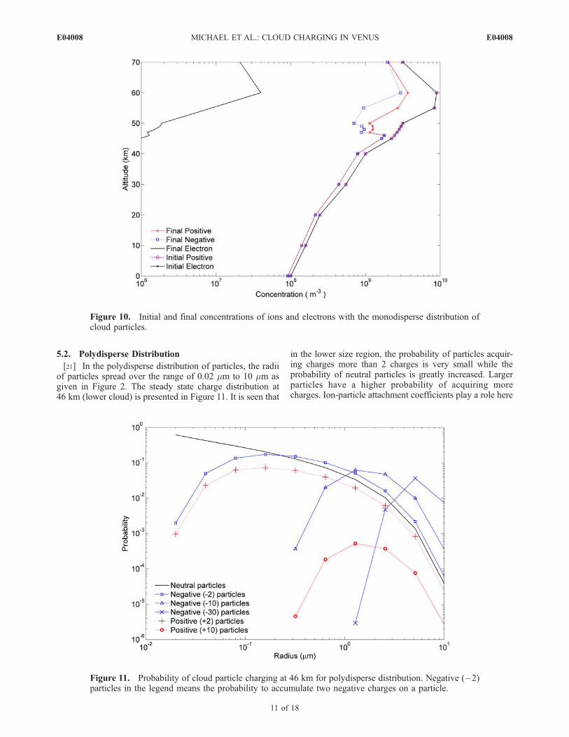
5.2. Polydisperse Distribution

[21] In the polydisperse distribution of particles, the radiiof particles spread over the range of 0.02 mm to 10 mm asgiven in Figure 2. The steady state charge distribution at46 km (lower cloud) is presented in Figure 11. It is seen that

in the lower size region, the probability of particles acquir-ing charges more than 2 charges is very small while theprobability of neutral particles is greatly increased. Largerparticles have a higher probability of acquiring morecharges. Ion-particle attachment coefficients play a role here

Figure 10. Initial and final concentrations of ions and electrons with the monodisperse distribution ofcloud particles.

Figure 11. Probability of cloud particle charging at 46 km for polydisperse distribution. Negative (�2)particles in the legend means the probability to accumulate two negative charges on a particle.


11 of 18

E04008

as for smaller particles the attachment coefficients are muchsmaller than that of the larger particles as depicted inFigures 6a–6c. The ratio of the charge on a particle to theradius of the particle is calculated and found that the ratio isalmost independent of the radius of the particle. It impliesthat larger particles accumulate greater number of charges astheir attachment coefficient is higher. It can also be notedthat more negatively charged particles are created thanpositively charged ones at all radius bins. The higherconcentration of negatively charged particles is attributedto the presence of highly mobile electrons, though in lowerabundance.[22] Figure 12 presents the contour of the charge distri-

bution of particles at 46 km. The color map is the logarithmof the concentration of particles. The charge distributionskews toward the negative side for bigger particles owing tothe presence of highly mobile electrons and also owing tothe higher attachment coefficients.[23] Figures 13 and 14 are similar to Figures 11 and 12

for 49 km (middle cloud). It is evident from Figure 13 thatthe probability of the bigger particles accumulating largenumber of charges is higher than that of smaller particlesowing to the higher attachment rates. The contour presentedin Figure 14 shows that the maximum concentration inclinestoward the negative side for larger particles owing to thepresence of highly mobile electrons. Chauzy and Despieu[1980] measured the charge accumulated by the rain dropsin the terrestrial atmosphere and found that larger dropscarried more negative charges.[24] Similarly, Figures 15 and 16 present the probability

of charging and the charge distribution at 55 km (uppercloud). It is clear from Figure 15 that even for particles of

size 0.1 mm, the probability of particles being negativelycharged is greater than that of remaining neutral, contrary tothat in the middle and lower cloud. This is due to thepresence of the highly mobile electron at a higher concen-tration at this altitude. All particles have a higher probabilityfor being negatively charged than positively charged. Thecontours in the Figure 16 show the very large negativecharges accumulated by the bigger particles.[25] Figure 17 presents the initial and final concentrations

of ions and electrons. The altitude profile is qualitativelysimilar to the case of monodisperse distribution and that ofBorucki et al. [1982]. The maximum reduction in the ionconcentration occurs at 50 km in agreement with that of themonodisperse case and that of Borucki et al. [1982].[26] The magnitude of reduction for the polydisperse case

is smaller (by a factor of 2 to 3) than that of the case ofmonodisperse distribution because the particles are distrib-uted over a wide range of radii and the resulting attachmentrate is much smaller than the case that assumes all theparticles are of bigger size. The effective attachment coef-ficient of the polydisperse particles was calculated andcompared with that of the monodisperse particles. It wasfound that the attachment rate for the monodisperse particleswas higher up to a factor of 6 than that of the polydispersecase.[27] Figure 18 presents the conductivity of the atmo-

sphere calculated using equation (8). To understand thesignificance of cloud particles, the calculations were carriedout in the presence and absence of particles. The conduc-tivity of the atmosphere with the monodisperse distributionof particles shows a similar trend to Borucki et al. [1982],where maximum reduction in conductivity occurs at

Figure 12. Charge distribution on cloud particles at 46 km with polydisperse distribution. The x axisrepresents the electronic charge on the particles. Color scale is the logarithm of the particle concentrationin m�3.


12 of 18

E04008

�50 km, with decreasing influence of cloud particles ataltitudes greater than 50 km. The magnitude of reductionin the conductivity at 50 km (factor of �3) is smaller inthe present work than reported by Borucki et al. [1982](� an order of magnitude). This is probably because the

total surface area of particles is about an order ofmagnitude less than that used by Borucki et al. [1982]which reduces the rate of attachment of ions to particles.[28] Another interesting aspect to note is that, with

polydisperse distribution of particles, the drop in conduc-

Figure 14. Charge distribution on cloud particles at 49 km with polydisperse distribution. The x axisrepresents the electronic charge on the particles. Color scale is the logarithm of the particle concentration.

Figure 13. Probability of cloud particle charging at 49 km for polydisperse distribution. Negative (�2)particles in the legend means the probability to accumulate two negative charges on a particle.


13 of 18

E04008

tivity is lesser than the monodisperse case. At 50 km, wherethe effect is maximum, the conductivity was reduced byonly about a factor of 2. The polydisperse distribution ofcloud particles, which is a more realistic scenario, considers

particles distributed over a size range of 0.02 mm to 10 mm,whereas in the monodisperse case all the particles are of thesize �8 mm. As the attachment coefficients are larger forbigger particles, the attachment rate is much larger, while

Figure 16. Charge distribution on cloud particles at 55 km with polydisperse distribution. The x axisrepresents the electronic charge on the particles. Color scale is the logarithm of the particle concentrationin m�3.

Figure 15. Probability of cloud particle charging at 55 km for polydisperse distribution.


14 of 18

E04008

using the monodisperse case. The effective attachmentcoefficients of the polydisperse distributed particles arefound to be less by factors of 6 to 2 in the altitude regionof 45 to 60 km compared to that of the monodispersedistributed particles. Though it is more convenient andcomputationally less expensive to use monodisperse distri-bution in the model, doing so overestimates the effect ofcloud particles on atmospheric conductivity.

[29] Rossow [1978] calculated the time constants for thecloud microphysical processes in the atmospheres of Earth,Venus, Mars and Jupiter. Carlson et al. [1988] used thesame method to calculate the time constants of predominantcloud microphysical processes in the atmospheres of giantplanets. The time constants for coagulation (>104 s), evap-oration (>105 s), sedimentation (>103 s) [Rossow, 1978], arefound to be greater than the time required for the charging to

Figure 17. Initial and final concentration of ions and electrons when the distribution of particles isconsidered polydisperse.

Figure 18. Altitude profile of conductivity for various conditions in the atmosphere of Venus.


15 of 18

E04008

reach the steady state (<103 s). Pruppacher and Klett [1997]estimated the time constant for cloud droplet charging byion diffusion close to the surface of the Earth as 400 s.Therefore the results presented would not be affected by theassumption of the same shape of the size distributionthroughout the charging calculation.

5.3. Implications for Lightning in the Atmosphere

[30] Russell et al. [2007] observed signals which appearto be due to the lightning from the clouds using a magne-tometer onboard Venus Express spacecraft. The signalsobtained occurred in bursts, with rapidly varying ampli-tudes, and variable interburst spacings and durations.Russell et al. [2007] reported observations of strong circu-larly polarized electromagnetic waves which appear asbursts of radiation lasting 0.25 to 0.5 s and have theexpected properties of whistler mode signals generated bylightning discharges in the clouds of Venus. The waveformsindicate an impulsive current source similar to terrestriallightning and also, the intermittent appearance of the burstsis like the occurrence pattern expected from a weather-associated phenomenon [Russell et al., 2007].[31] Figure 19 presents the ratio of positive to negative

charges acquired by the droplets of different sizes. It can beseen that in the lower cloud region the charge ratio is similarfor particles of size less than 0.06 mm, whereas the ratiobecomes much larger for larger particles in the middle andupper cloud regions. This suggests that there are morenegatively charged particles in the middle and upper cloudregion compared to the lower cloud region. As mentionedearlier, generation of more negatively charged particles atgreater altitudes is due to the presence of larger concentra-tion of highly mobile electrons, which get easily attached toparticles, especially larger ones. It is clearly visible fromFigure 19 that the ratio of the positive to negative charges

shows a steep decrease for altitudes greater than 50 km andbecomes saturated or changes direction for altitudes greaterthan 60 km. The occurrence of such a large charge separa-tion is in agreement with the suggestion of Russell et al.[2006] that the middle cloud droplets can be charged likethe cloud droplets on the terrestrial atmosphere where thetemperature and pressure are similar. If vertical winds exist,then large particles can be physically separated from thesmall and an electric field will be generated. The electricfield will build to the point where one of two situationsoccurs; either the electric current caused by the electric fieldlimits the electric field to a value below the breakdownvalue, or the electric field exceeds that value and anelectrical discharge occurs. An order of magnitude calcula-tion given below shows that lightning discharges in the 40to 70 km altitude range is highly unlikely.[32] For the pressure range of interest, breakdown electric

fields will be of the order 105 to 106 volts m�1 [Roussel-Dupre et al., 2008], which is similar to the terrestrialatmosphere. On the basis of the conductivities calculated(i.e., �10�13 ohm�1 m�1), the corresponding leakagecurrents would be 10�8 to 10�7 Am�2. To reach thebreakdown electric field, the charging current must exceedthe leakage current. Even if the entire formation rate ofelectrons by GCR (�3 � 107 e s�1 m�3) went into chargingthe small aerosols and the vertical wind were just largeenough (i.e., 2 � 10�3 m s�1) to levitate the small aerosolswithout levitating the large 4 mm radius particles, thecharging current would be no larger than 10�14 Am�2,many orders of magnitude too low to generate the electricfield necessary for a lightning discharge. In the horizontaldirection also, there is no obvious mechanisms to providethe work required to separate charges and, therefore, alightning discharge is not expected.

Figure 19. Ratio of total positive to negative charges accumulated on the cloud particles.


16 of 18

E04008

[33] Tzur and Levin [1982] modeled the electric field nearthe surface of Venus by diffusion and conduction currents. Itwas found that a maximum of 30 Vm�1 can be produced bydiffusion at the surface and expected that if there is a chargeseparation within the cloud layers, it can affect the magni-tude of the field [Tzur and Levin, 1982]. As the chargingprocess studied here is more rapid than the particle-particleinteraction and vertical transport, such a charge separationand development of electric field which can activate light-ning seems unlikely in the atmosphere of Venus.

6. Conclusions

[34] Charging of cloud droplets in the atmosphere ofVenus is examined in the present work. Charging occursby the charge transfer by ions and attachment of electrons tothe particles. GCR are the major source of ions andelectrons in the altitudes of interest. Charge balance equa-tions are constructed to estimate the steady state concentra-tion of ions, electrons and particles which are charged aswell as neutral. Both monodisperse and polydisperse dis-tributions of particles were used and the results werecompared. The present results compare favorably with thoseof Borucki et al. [1982] when the differences of aerosolproperties are considered.[35] The following are the major conclusions of the study:

(1) Large number of charges are accumulated on particles inthe altitude region 48 to 55 km because of the existence oflarger sizes and greater concentration of particles. (2)Maximum reduction in ion concentration (at 50 km) wasfound to be a factor of 5 for monodisperse distribution ofparticles in the cloud layer, while Borucki et al. [1982]observed a maximum drop of an order of magnitude due tothe higher surface area of the particles used in thosecalculations. (3) For polydisperse distribution of particles,the maximum reduction in ion concentration was found tobe only a factor of 3, as the effective attachment coefficientsof the polydisperse particles are lower than those of mono-disperse distributed particles. (4) Therefore, monodispersedistribution overestimates the reduction in conductivity,though it is more convenient and computationally lessexpensive than the more realistic polydisperse distributionof particles. (5) Charging of aerosols by energetic particlesand the separation of charge due to differential charging andvertical winds appears to be inadequate to generate theelectric fields necessary to cause the lightning events someinvestigators have observed.

ReferencesAplin, K. (2006), Atmospheric electrification in the solar system, Surv.Geophys., 27, 63–108, doi:10.1007/s10712-005-0642-9.

Arnold, H. R. (1964), Comments on a paper, ‘‘Collisional detachment andthe formation of an ionospheric C region’’ by Pierce, E.T., J. Res. Natl.Bur. Stand. U.S., Sect. D, 68, 215–217.

Bell, J. F., III, D. Crisp, P. G. Lucey, T. A. Ozorski, W. M. Sinton, S. C.Willis, and B. A. Campbell (1991), Spectroscopic observations of brightand dark emission features on the night side of Venus, Science, 252,1293–1296, doi:10.1126/science.252.5010.1293.

Bertaux, J. L., et al. (2007), SPICAV on Venus Express: Three spectro-meters to study the global structure and composition of the Venus atmo-sphere, Planet. Space Sci., 55, 1673 – 1700, doi:10.1016/j.pss.2007.01.016.

Borucki, W. J., Z. Levin, R. C. Whitten, R. G. Keesee, L. A. Capone, O. B.Toon, and J. Dubach (1982), Predicted electrical conductivity between 0and 80 km in the Venusian atmosphere, Icarus, 51, 302 – 321,doi:10.1016/0019-1035(82)90086-0.

Borucki, W. J., J. W. Dyer, J. R. Phillips, and P. Pham (1991), PioneerVenus orbiter search for Venusian lightning, J. Geophys. Res., 96,11,033–11,043, doi:10.1029/91JA01097.

Borucki, W. J., R. C. Whitten, E. L. O. Bakes, E. Barth, and S. N. Tripathi(2006), Predictions of the electrical conductivity and charging of theaerosols in Titan’s atmosphere 6/20/05, Icarus, 181, 527 – 544,doi:10.1016/j.icarus.2005.10.030.

Carlson, B. E., W. B. Rossow, and G. S. Orton (1988), Cloud microphysicsof giant planets, J. Atmos. Sci., 45, 2066–2081, doi:10.1175/1520-0469(1988)045<2066:CMOTGP>2.0.CO;2.

Carlson, R. W., L. W. Kamp, K. H. Baines, J. B. Pollack, D. H. Grinspoon,T. Encrenaz, P. Drossart, and F. W. Taylor (1993), Variations in Venuscloud particle properties: A new view of Venus’s cloud morphology asobserved by the Galileo near-infrared mapping spectrometer, Planet.Space Sci., 41, 477–485.

Chauzy, S., and S. Despieu (1980), Rainfall rate and electric charge and sizeof raindrops of six spring showers, J. Atmos. Sci., 37, 1619–1627,doi:10.1175/1520-0469(1980)037<1619:RRAECA>2.0.CO;2.

Chen, R. H., and A. F. Nagy (1978), A comprehensive model of the Venusionosphere, J. Geophys. Res. , 83 , 1133 – 1140, doi:10.1029/JA083iA03p01133.

Christophorou, L. G. (1980), Negative ions of polyatomic molecules,Environ. Health Perspect., 36, 3–32, doi:10.2307/3429329.

Crisp, D., et al. (1989), The nature of the near-infrared features on theVenus night side, Science, 246, 506 – 509, doi:10.1126/science.246.4929.506.

Crisp, D., et al. (1991), Ground-based near-infrared imaging observationsof Venus during the Galileo encounter, Science, 253, 1538 –1541,doi:10.1126/science.253.5027.1538.

Desch, S. J., W. J. Borucki, C. T. Russell, and A. Bar-Nun (2002), Progressin planetary lightning, Rep. Prog. Phys., 65, 955–997, doi:10.1088/0034-4885/65/6/202.

Esposito, L. W., R. G. Knollenberg, M. Y. Marov, O. B. Toon, and R. P.Turco (1983), The clouds and hazes of Venus, in Venus, edited by D. M.Hunten et al., pp. 484–564, Univ. of Ariz. Press, Tucson.

Grinspoon, D. H., J. B. Pollack, B. R. Sitton, R. W. Carlson, L. W. Kamp,K. H. Baines, T. Encrenaz, and F. W. Taylor (1993), Probing Venus’scloud structure with Galileo NIMS, Planet. Space Sci., 41, 515–542.

Gurnett, D. A., W. S. Kurth, A. Roux, R. Gendrin, C. F. Kennel, and S. J.Bolton (1991), Lightning and plasma wave observations from the Galileoflyby of Venus, Science, 253, 1522 – 1525, doi:10.1126/science.253.5027.1522.

Gurnett, D. A., P. Zarka, R. Manning, W. S. Kurth, G. B. Hospodarsky, T. F.Averkamp, M. L. Kaiser, and W. M. Farrell (2001), Non-detection atVenus of high-frequency radio signals characteristic of terrestrial light-ning, Nature, 409, 313–315, doi:10.1038/35053009.

Hansell, S. A., W. K. Wells, and D. M. Hunten (1995), Optical detection oflightning on Venus, Icarus, 117, 345–351, doi:10.1006/icar.1995.1160.

Hansen, J. E., and J. W. Hovenier (1974), Interpretation of the polarizationof Venus, J. Atmos. Sci., 31, 1137–1160, doi:10.1175/1520-0469(1974)031<1137:IOTPOV>2.0.CO;2.

Hoppel, W. A. (1985), Ion-aerosol attachment coefficients, ion depletion,and the charge distribution on aerosols, J. Geophys. Res., 90, 5917–5923,doi:10.1029/JD090iD04p05917.

Hoppel, W. A., and G. M. Frick (1986), Ion-aerosol attachment coefficientsand the steady-state charge on aerosols in a bipolar ion environment,Aerosol Sci. Technol., 5, 1–21, doi:10.1080/02786828608959073.

Hua, H., and R. H. Holzworth (1996), Observations and parameterizationof the stratospheric electrical conductivity, J. Geophys. Res., 101,29,539–29,552, doi:10.1029/96JD01060.

Imamura, T., and G. L. Hashimoto (1998), Venus cloud formation in themeridional circulation, J. Geophys. Res., 103, 31,349 – 31,366,doi:10.1029/1998JE900010.

Imamura, T., and G. L. Hashimoto (2001), Microphysics of Venusianclouds in rising tropical air, J. Atmos. Sci., 58, 3597 – 3612,doi:10.1175/1520-0469(2001)058<3597:MOVCIR>2.0.CO;2.

James, E. P., O. B. Toon, and G. Schubert (1997), A numerical microphy-sical model of the condensational Venus cloud, Icarus, 129, 147–171,doi:10.1006/icar.1997.5763.

Jensen, E. J., and G. E. Thomas (1991), Charging of mesospheric particles:Implications for electron density and particle coagulation, J. Geophys.Res., 96, 18,603–18,615, doi:10.1029/91JD01966.

Kawabata, K., D. L. Coffeen, J. E. Hansen, W. A. Lane, M. Sato, andL. D. Travis (1980), Cloud and haze properties from Pioneer Venuspolarimetry, J. Geophys. Res., 85, 8129 – 8140, doi:10.1029/JA085iA13p08129.

Keesee, R. G., N. Lee, and A. W. Castleman Jr. (1980), Properties ofclusters in the gas phase: V. Complexes of neutral molecules onto nega-tive ions, J. Chem. Phys., 73, 2195–2202, doi:10.1063/1.440415.


17 of 18

E04008

Knollenberg, R. G., and D. M. Hunten (1980), The microphysics of theclouds of Venus: Results of the Pioneer Venus particle size spectrometerexperiment, J. Geophys. Res. , 85 , 8039 – 8058, doi:10.1029/JA085iA13p08039.

Krasnopolsky, V. A. (1983), Lightning and nitric oxide on Venus, Planet.Space Sci., 31, 1363–1369, doi:10.1016/0032-0633(83)90072-7.

Krasnopolsky, V. A. (1989), Vega mission results and chemical compositionof Venusian clouds, Icarus, 80, 202 – 210, doi:10.1016/0019-1035(89)90168-1.

Krasnopolsky, V. A. (2007), Chemical kinetic model for the lower atmo-sphere of Venus, Icarus, 191, 25–37, doi:10.1016/j.icarus.2007.04.028.

Krasnopolsky, V. A., and J. B. Pollack (1994), H2O-H2SO4 system inVenus’ clouds and OCS, CO, and H2SO4 profiles in Venus’ troposphere,Icarus, 109, 58–78, doi:10.1006/icar.1994.1077.

Markiewicz, W. J., et al. (2007), Morphology and dynamics of the uppercloud layer of Venus, Nature, 450, doi:10.1038/nature06320.

Michael, M., and S. N. Tripathi (2008), Effect of charging of aerosols in thelower atmosphere of mars during the dust storm of 2001, Planet. SpaceSci., 56, 1696–1702, doi:10.1016/j.pss.2008.07.030.

Michael, M., M. Barani, and S. N. Tripathi (2007), Numerical predictionsof aerosol charging and electrical conductivity of the lower atmosphere ofMars, Geophys. Res. Lett., 34, L04201, doi:10.1029/2006GL028434.

Michael, M., S. N. Tripathi, and S. K. Mishra (2008), Dust charging andelectrical conductivity in the day and night-time atmosphere of Mars,J. Geophys. Res., 113, E07010, doi:10.1029/2007JE003047.

Mills, F. P., and M. Allen (2007), A review of selected issues concerningthe chemistry in Venus’ middle atmosphere, Planet. Space Sci., 55,1729–1740, doi:10.1016/j.pss.2007.01.012.

O’ Brien, K. (1970), Calculated cosmic ray ionization in the loweratmosphere, J. Geophys. Res., 75, 4357 – 4359, doi:10.1029/JA075i022p04357.

Parthasarathy, R. (1976), Mesopause dust as a sink for ionization, J. Geo-phys. Res., 81, 2392–2396.

Pollack, J. B., D. W. Strecker, F. C. Witteborn, E. F. Erickson, and B. J.Baldwin (1978), Properties of the clouds of Venus, as inferred from air-borne observations of its near-infrared reflectivity spectrum, Icarus, 34,28–45.

Pollack, J. B., et al. (1993), Near infrared light from Venus’ nightside: Aspectroscopic analysis, Icarus, 103, 1–42, doi:10.1006/icar.1993.1055.

Pruppacher, H. R., and J. D. Klett (1997), Microphysics of Clouds andPrecipitation, 2nd ed., Kluwer Acad., Dordrecht, Netherlands.

Rossow, W. B. (1978), Cloud microphysics: Analysis of the clouds ofEarth, Venus, Mars, and Jupiter, Icarus, 36, 1–50, doi:10.1016/0019-1035(78)90072-6.

Roussel-Dupre, R., J. J. Colman, E. Symbalisty, D. Sentman, and V. P.Pasko (2008), Physical processes related to discharges in planetary atmo-spheres, Space Sci. Rev., 137, 51–82, doi:10.1007/s11214-008-9385-5.

Russell, C. T. (1991), Venus lightning, Space Sci. Rev., 55, 317–356.Russell, C. T., R. J. Strangeway, and T. L. Zhang (2006), Lightning detec-tion on the Venus Express mission, Planet. Space Sci., 54, 1344–1351,doi:10.1016/j.pss.2006.04.026.

Russell, C. T., T. L. Zhang, M. Delva, W. Magnes, R. J. Strangeway, andH. Y. Wei (2007), Lightning on Venus inferred from whistler-mode wavesin the ionosphere, Nature, 450, 661–662, doi:10.1038/nature05930.

Sagdeev, R. Z., et al. (1986), Overview of VEGA Venus balloon in situmeteorological measurements, Science, 231, 1411–1414, doi:10.1126/science.231.4744.1411.

Taylor, F. W., et al. (1980), Structure and meteorology of the middleatmosphere of Venus: Infrared remote sensing from the Pioneer orbiter,J. Geophys. Res., 85, 7963–8006, doi:10.1029/JA085iA13p07963.

Tinsley, B. A., and L. Zhou (2006), Initial results of a global circuit modelwith variable stratospheric and tropospheric aerosols, J. Geophys. Res.,111, D16205, doi:10.1029/2005JD006988.

Toon, O. B., R. P. Turco, and J. B. Pollack (1982), The ultraviolet absorberon Venus: Amorphous sulfur, Icarus, 51, 358–373, doi:10.1016/0019-1035(82)90089-6.

Tripathi, S. N., and M. Michael (2008), Aerosols in the atmosphere ofMars, in Modeling of Planetary Atmosphere, edited by S. A. Haideret al., chap. 3, Macmillan, India, in press.

Tripathi, S. N., M. Michael, and R. G. Harrison (2008), Profiles of ionand aerosol interactions in planetary atmospheres, Space Sci. Rev., 137,193–211, doi:10.1007/s11214-008-9367-7.

Turco, R. P., O. B. Toon, R. C. Whitten, and R. G. Keesee (1983), Venus:Mesospheric hazes of ice, dust, and acid aerosols, Icarus, 53, 18–25,doi:10.1016/0019-1035(83)90017-9.

Tzur, I., and Z. Levin (1982), A one-dimensional model of the atmosphericelectric field near the Venusian surface, Icarus, 52, 346 – 353,doi:10.1016/0019-1035(82)90117-8.

Upadhyay, H. O., R. R. Singh, and R. N. Singh (1994), Cosmic ray ioniza-tion of lower Venus atmosphere, Earth Moon Planets, 65, 89 –94,doi:10.1007/BF00572202.

Whitten, R. C., W. J. Borucki, and S. N. Tripathi (2007), Predictions of theelectrical conductivity and charging of the aerosols in Titan’s nighttimeatmosphere, J. Geophys. Res., 112, E04001, doi:10.1029/2006JE002788.

Whitten, R. C., W. J. Borucki, and S. N. Tripathi (2008), Predictions of theelectrical conductivity and charging of the cloud particles in Jupiter’satmosphere, J. Geophys. Res., 113, E04001, doi:10.1029/2007JE002975.

Yair, Y., and Z. Levin (1989), Charging of polydispersed aerosol particlesby attachment of atmospheric ions, J. Geophys. Res., 94, 13,085–13,091,doi:10.1029/JD094iD11p13085.

Yair, Y., G. Fischer, F. Simoes, N. Renno, and P. Zarka (2008), Updatedreview of planetary atmospheric electricity, Space Sci. Rev., 137, 29–49,doi:10.1007/s11214-008-9349-9.

Yamamoto, M., and M. Takahashi (2006), An aerosol transport modelbased on a two-moment microphysical parameterization in the Venusmiddle atmosphere: Model description and preliminary experiments,J. Geophys. Res., 111, E08002, doi:10.1029/2006JE002688.

Young, A. T. (1973), Are the clouds of Venus sulfuric acid?, Icarus, 18,564–582, doi:10.1016/0019-1035(73)90059-6.

��W. J. Borucki, NASA Ames Research Center, Moffett Field, CA 94035,

USA.M. Michael and S. N. Tripathi, Department of Civil Engineering, Indian

Institute of Technology, Kanpur 208016, India. ([email protected])R. C. Whitten, SETI Research Institute, 515 N. Whisman Road,

Mountain View, CA 94043, USA.


18 of 18

E04008

Documents

Highly charged cloud particles in the atmosphere of Venushome.iitk.ac.in/~snt/pdf/Michael_VenusCloudCharging.pdf · Highly charged cloud particles in the atmosphere of Venus ... W