An Introduction to Charged Particles Trackingphysics.iitm.ac.in/~sercehep2013/track2_Gagan_Mohanty.pdf · An Introduction to Charged Particles Tracking – Francesco Ragusa 4 Magnetic

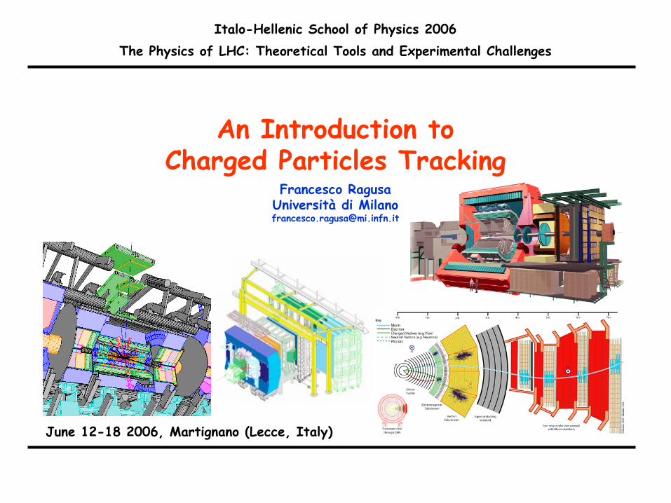
An Introduction to Charged Particles Tracking

Francesco RagusaUniversità di [email protected]

Italo-Hellenic School of Physics 2006The Physics of LHC: Theoretical Tools and Experimental Challenges

June 12-18 2006, Martignano (Lecce, Italy)

An Introduction to Charged Particles Tracking – Francesco Ragusa 1

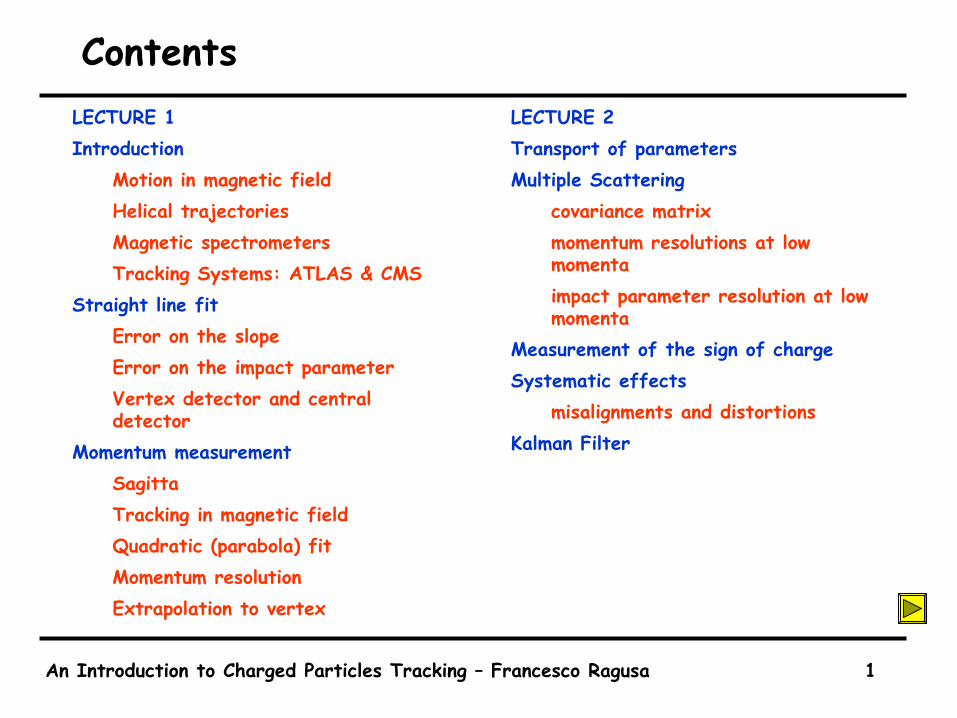
ContentsLECTURE 1Introduction

Motion in magnetic fieldHelical trajectoriesMagnetic spectrometersTracking Systems: ATLAS & CMS

Straight line fitError on the slopeError on the impact parameterVertex detector and central detector

Momentum measurementSagittaTracking in magnetic fieldQuadratic (parabola) fitMomentum resolutionExtrapolation to vertex

LECTURE 2Transport of parametersMultiple Scattering

covariance matrixmomentum resolutions at low momentaimpact parameter resolution at low momenta

Measurement of the sign of chargeSystematic effects

misalignments and distortionsKalman Filter


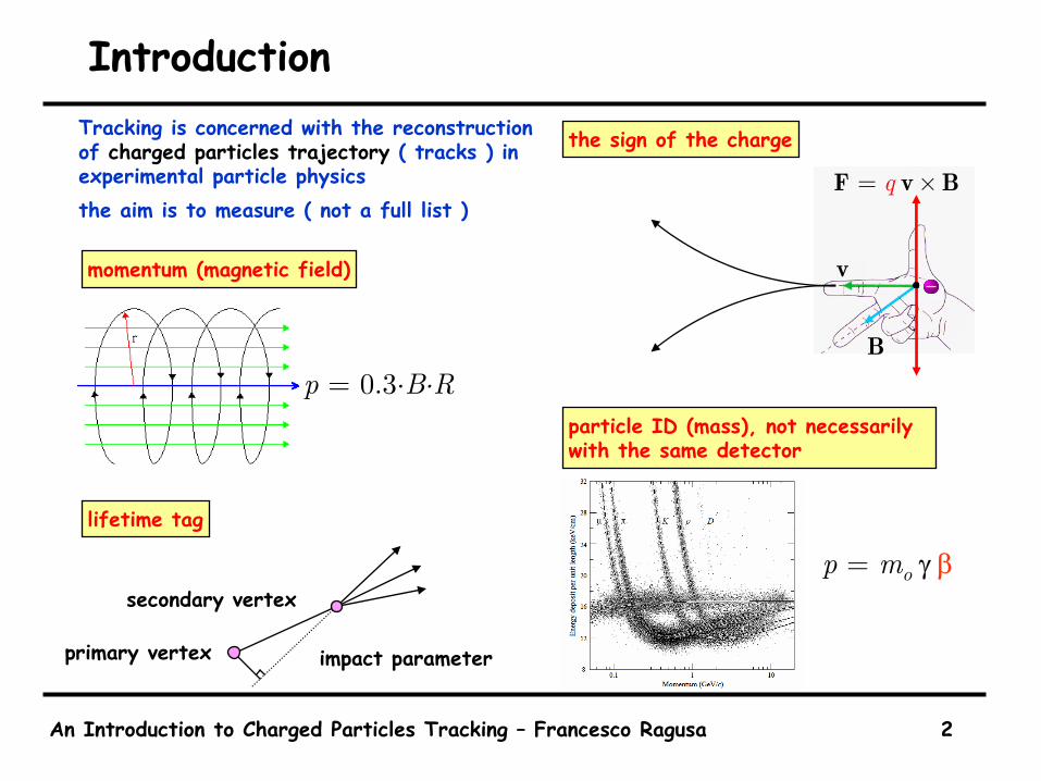
IntroductionTracking is concerned with the reconstruction of charged particles trajectory ( tracks ) in experimental particle physicsthe aim is to measure ( not a full list )

momentum (magnetic field)

the sign of the charge

particle ID (mass), not necessarily with the same detector

p = mo γ βsecondary vertex

primary vertex

lifetime tag

q= ×F v B

v

Bp = 0.3·B·R

impact parameter


Motion in Magnetic FieldIn a magnetic field the motion of a char-ged particle is determined by the Lorentz Force

Since magnetic forces do not change the energy of the particle

using the path length s along the track instead of the time t

we have

and finally

In case of inhomogeneus magnetic field, B(s) varies along the track and to find the trajectory r(s) one has to solve a differential equationIn case of homogeneus magnetic field the trajectory is given by an helix

d edt= ×p v B

odm edt

γ = ×v v B

2

2od dm e

dtdtγ = ×r r B

ds vdt=

2

2od dm v e

dsdsγ = ×r r B

2

2d e d

p dsds= ×r r B

B

vz

vs v


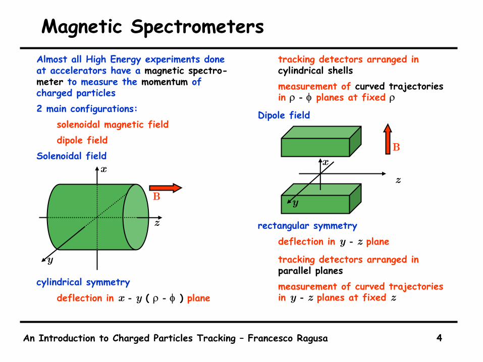
Magnetic SpectrometersAlmost all High Energy experiments done at accelerators have a magnetic spectro-meter to measure the momentum of charged particles2 main configurations:

solenoidal magnetic fielddipole field

Solenoidal field

cylindrical symmetrydeflection in x - y ( ρ - φ ) plane

tracking detectors arranged in cylindrical shellsmeasurement of curved trajectoriesin ρ - φ planes at fixed ρ

Dipole field

rectangular symmetrydeflection in y - z plane

tracking detectors arranged in parallel planesmeasurement of curved trajectories in y - z planes at fixed z

z

x

y

Bz

y

xB


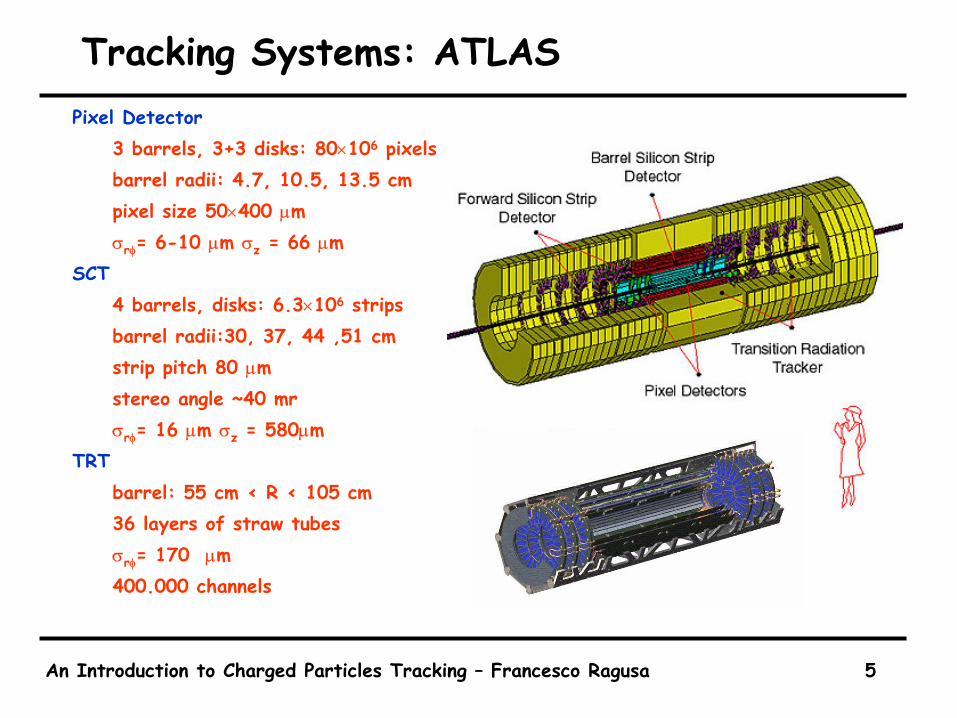
Tracking Systems: ATLASPixel Detector

3 barrels, 3+3 disks: 80×106 pixelsbarrel radii: 4.7, 10.5, 13.5 cmpixel size 50×400 µmσrφ= 6-10 µm σz = 66 µm

SCT4 barrels, disks: 6.3×106 stripsbarrel radii:30, 37, 44 ,51 cmstrip pitch 80 µm stereo angle ~40 mr σrφ= 16 µm σz = 580µm

TRTbarrel: 55 cm < R < 105 cm36 layers of straw tubesσrφ= 170 µm400.000 channels


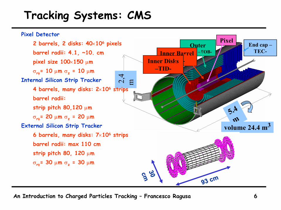
Tracking Systems: CMS

5.4

m

OuterBarrel –TOB-Inner Barrel

–TIB-

End cap –TEC-

Pixel

2,4

mvolume 24.4 m3

Inner Disks –TID-

93 cm93 cm

30 30 cmcm

Pixel Detector2 barrels, 2 disks: 40×106 pixelsbarrel radii: 4.1, ~10. cmpixel size 100×150 µmσrφ= 10 µm σz = 10 µm

Internal Silicon Strip Tracker4 barrels, many disks: 2×106 stripsbarrel radii:strip pitch 80,120 µmσrφ= 20 µm σz = 20 µm

External Silicon Strip Tracker6 barrels, many disks: 7×106 stripsbarrel radii: max 110 cmstrip pitch 80, 120 µmσrφ= 30 µm σz = 30 µm


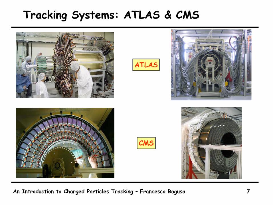
Tracking Systems: ATLAS & CMS

ATLAS

CMS


Momentum MeasurementThe momentum of the particle is projected along two directions

in ρ - φ plane we measure the transverse momentum

in the ρ - z plane we measure the dip angle λ

orders of magnitude

the sagitta s

assume a track length of 1 m

⊥P

cos 0.3P P BRλ⊥ = = 2α

R

s

2 LR

α =

( )1 coss R α= −2 2

2 8Ls RR

α≈ =

1 2 1.67

10 2 16.7

P GeV B T R m

P GeV B T R m⊥

⊥

= = =

= = =

ρ

φ

1 7.4

10 0.74

P GeV s cm

P GeV s cm⊥

⊥

= =

= =λ

ρ

z

λ

P

⊥P

LPρ

z


Momentum MeasurementOnce we have measured the transversemomentum and the dip angle the totalmomentum is

the error on the momentum is easely calculated

We need to studythe error on the radius measured in the bending plane ρ - φ

the error on the dip angle in theρ - z plane

We need to study alsocontrubution of multiple scattering to momentum resolution

Comment:in an hadronic collider the main emphasis is on transverse momentumelementary processes among partons that are not at rest in the laboratory frameuse of momentum conservation only in the transverse plane

0.3cos cosP BRP

λ λ⊥= =

PPR R

⊥∂ =∂

tanP P λλ ⊥

∂ = −∂

( )2 2

2tanP RP R

λ λ∆ ∆ = + ∆


The Helix EquationThe helix is described in parametric form

λ is the dip angleh =±1 is the sense of rotation on the helixThe projection on th x-y plane is a circle

xo and yo the coordinates at s = 0

Φo is also related to the slope of the tangent to the circle at s = 0

( ) ( )coscos coso o ohsx s x RR

λ = + Φ + − Φ

( ) ( )cossin sino o ohsy s y RR

λ = + Φ + − Φ

( ) sinoz s z s λ= +

( ) ( )2 2 2cos sino o o ox x R y y R R− + Φ + − + Φ =

cos oR Φ

( ),o ox y

oΦ

sin oR Φ

( )( )( )0.3

p GeVR m

B T⊥=

B

λ

P⊥P

LP


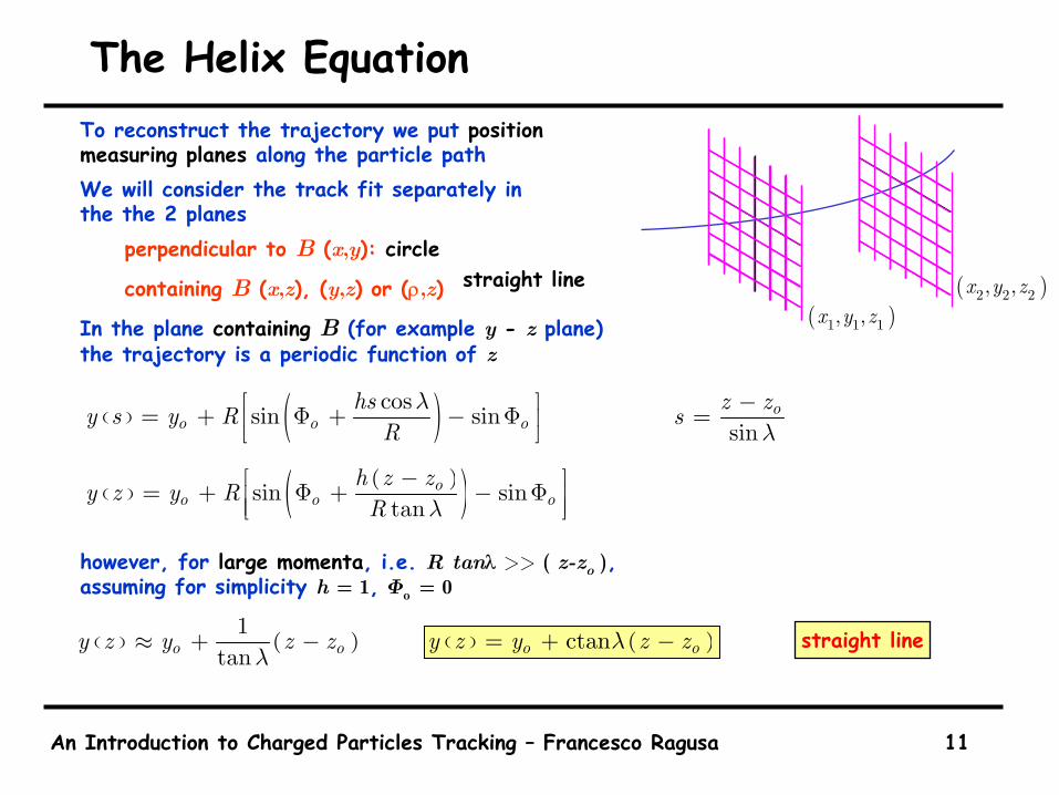
The Helix EquationTo reconstruct the trajectory we put positionmeasuring planes along the particle pathWe will consider the track fit separately in the the 2 planes

perpendicular to B (x,y): circle

containing B (x,z), (y,z) or (ρ,z)

In the plane containing B (for example y - z plane) the trajectory is a periodic function of z

however, for large momenta, i.e. R tanλ >> ( z-zo ), assuming for simplicity h = 1, Φo = 0

sinoz zsλ

−=

( )( )( )sin sin

tano

o o oh z zy z y RR λ

− = + Φ + − Φ

( ) ( )1

tano oy z y z zλ

≈ + −

( ) ( )cossin sino o ohsy s y RR

λ = + Φ + − Φ

( )1 1 1, ,x y z( )2 2 2, ,x y z

( ) ( )ctano oy z y z zλ= + −

straight line

straight line


The Helix Equation


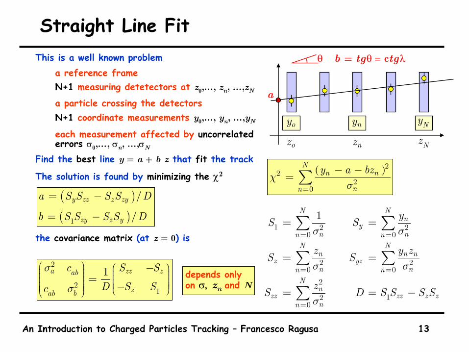
Straight Line FitThis is a well known problem

a reference frameN+1 measuring detetectors at z0,…, zn, …,zN

a particle crossing the detectorsN+1 coordinate measurements y0,…, yn, …,yN

each measurement affected by uncorrelatederrors σ0,…, σn, …,σN

Find the best line y = a + b z that fit the track

The solution is found by minimizing the χ2

the covariance matrix (at z = 0) is

oz nz NzNyoy ny

( )222

0

Nn n

nn

y a bzχσ=

− −= ∑( )( )1

/

/

y zz z zy

zy z y

a S S S S D

b S S S S D

= −

= −

2

21

1a zz zab

zab b

c S S

D S Sc

σ

σ

− = −

1 2 20 0

2 20 0

2

120

1N Nn

yn nn n

N Nn n n

z yzn nn n

Nn

zz zz z znn

yS S

z y zS S

zS D S S S S

σ σ

σ σ

σ

= =

= =

=

= =

= =

= = −

∑ ∑

∑ ∑

∑

a

θ b = tgθ = ctgλ

depends onlyon σ, zn and N


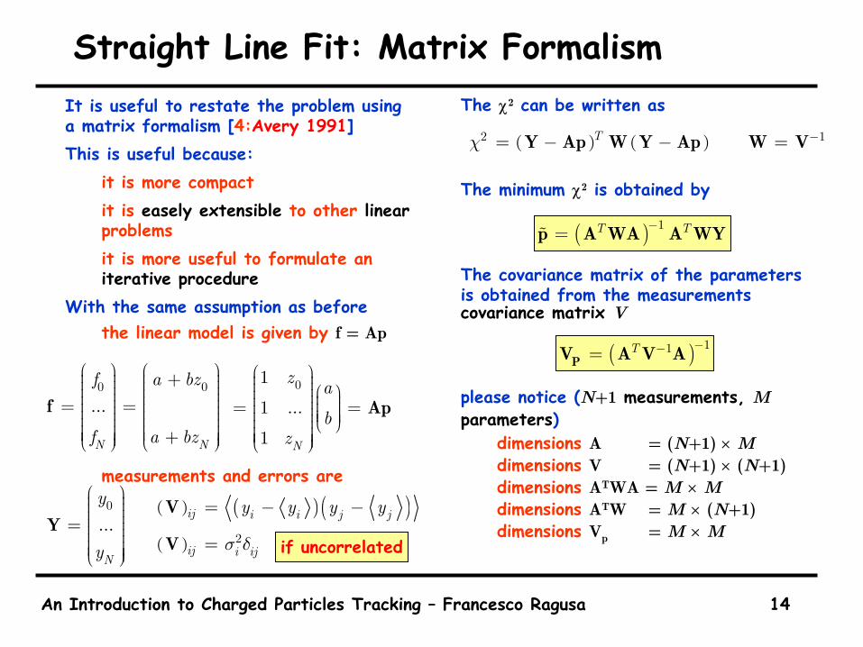
Straight Line Fit: Matrix FormalismIt is useful to restate the problem using a matrix formalism [4:Avery 1991]This is useful because:

it is more compactit is easely extensible to other linearproblemsit is more useful to formulate an iterative procedure

With the same assumption as beforethe linear model is given by f = Ap

measurements and errors are

The χ2 can be written as

The minimum χ2 is obtained by

The covariance matrix of the parameters is obtained from the measurements covariance matrix V

please notice (N+1 measurements, Mparameters)

dimensions A = (N+1) × Mdimensions V = (N+1) × (N+1)dimensions ATWA = M × Mdimensions ATW = M × (N+1)dimensions Vp = M × M

0 0

...

N N

f a bz

f a bz

+ = = +

f

0

...

N

y

y

=

Y

( ) ( )2 1Tχ −= − − =Y Ap W Y Ap W V

( ) 1T T−=p A WA A WY

( ) 11T −−=PV A V A01

1 ...

1 N

z a

bz

= =

Ap

( ) ( )( )ij i i j jy y y y= − −V

( ) 2ij i ijσ δ=V if uncorrelated


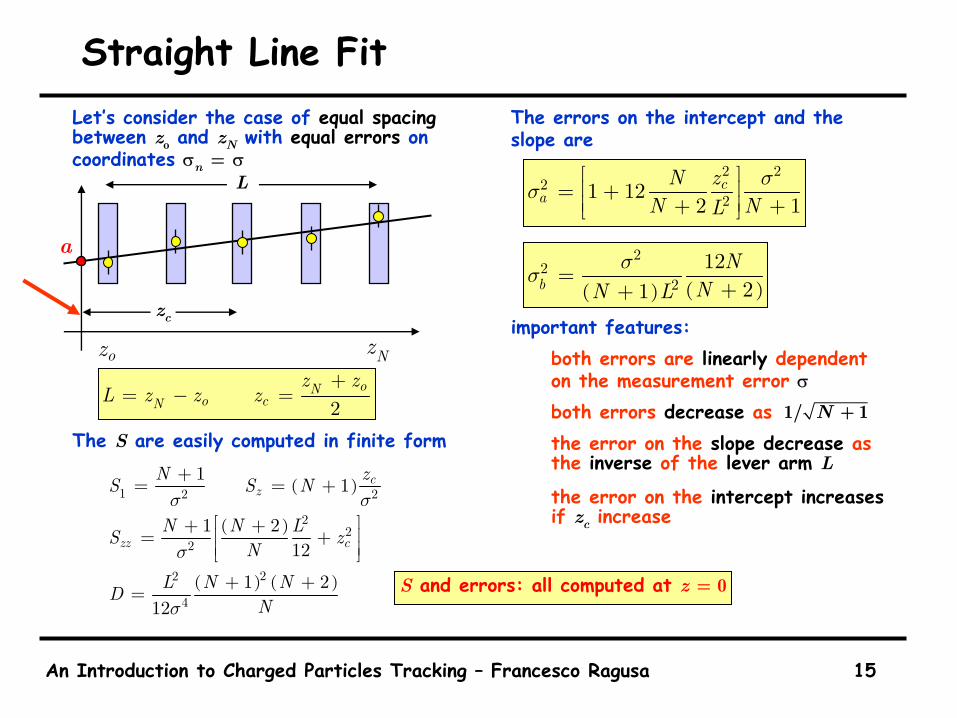
Straight Line FitLet’s consider the case of equal spacingbetween zo and zN with equal errors on coordinates σn = σ

The S are easily computed in finite form

The errors on the intercept and the slope are

important features:both errors are linearly dependent on the measurement error σ

both errors decrease as the error on the slope decrease as the inverse of the lever arm L

the error on the intercept increasesif zc increase

oz Nz

( )

( )

( ) ( )

1 2 2

22

2

22

4

1 1

1 212

1 212

cz

zz c

N zS S N

N N LS zN

L N NDN

σ σ

σ

σ

+= = +

+ + = + + +=

2oN

o cNz z

L z z z+

= − =

L

zc

2 22

21 122 1c

aN zN NL

σσ = + + +

( ) ( )

22

212

21bN

NN Lσσ =

++

1/ + 1N

S and errors: all computed at z = 0

a


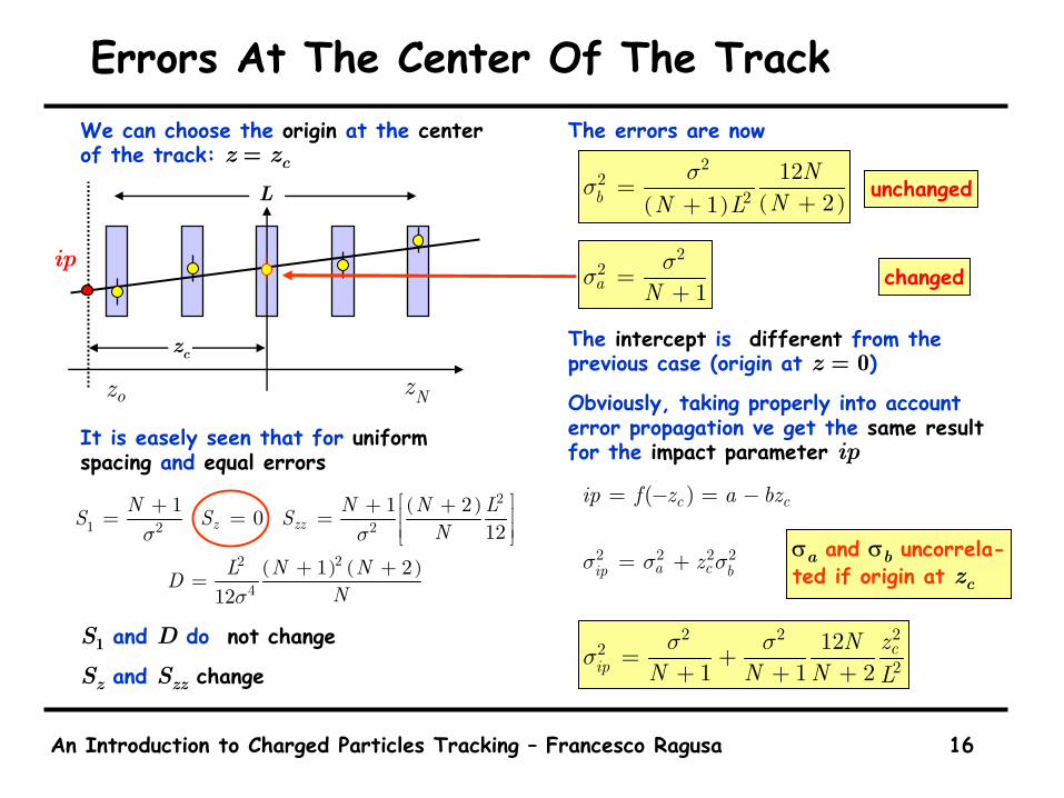
Errors At The Center Of The TrackWe can choose the origin at the centerof the track: z = zc

It is easely seen that for uniformspacing and equal errors

S1 and D do not change

Sz and Szz change

The errors are now

The intercept is different from the previous case (origin at z = 0)Obviously, taking properly into account error propagation ve get the same resultfor the impact parameter ip

( )

( ) ( )

2

1 2 2

22

4

1 1 2012

1 212

z zzN N N LS S S

N

L N NDN

σ σ

σ

+ + + = = = + +=

22

1a Nσσ =+

( ) ( )

22

212

21bN

NN Lσσ =

++

changed

unchanged

( )c cip f z a bz= − = −

L

zc

oz Nz

ip

2 2 2 2a cip bzσ σ σ= +

2 2 22

212

1 1 2c

ipN z

N N N Lσ σσ = ++ + +

σa and σb uncorrela-ted if origin at zc


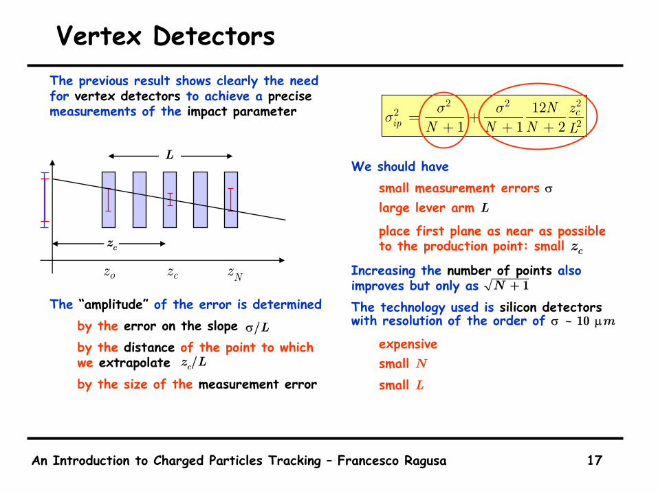
Vertex DetectorsThe previous result shows clearly the need for vertex detectors to achieve a precisemeasurements of the impact parameter

The “amplitude” of the error is determinedby the error on the slopeby the distance of the point to which we extrapolateby the size of the measurement error

We should havesmall measurement errors σ

large lever arm L

place first plane as near as possible to the production point: small zc

Increasing the number of points also improves but only asThe technology used is silicon detectors with resolution of the order of σ ~ 10 µm

expensivesmall Nsmall L

oz Nzcz

L

zc

σ/L

zc/L

+ 1N

2 2 22

212

1 1 2c

ipN z

N N N Lσ σσ = ++ + +


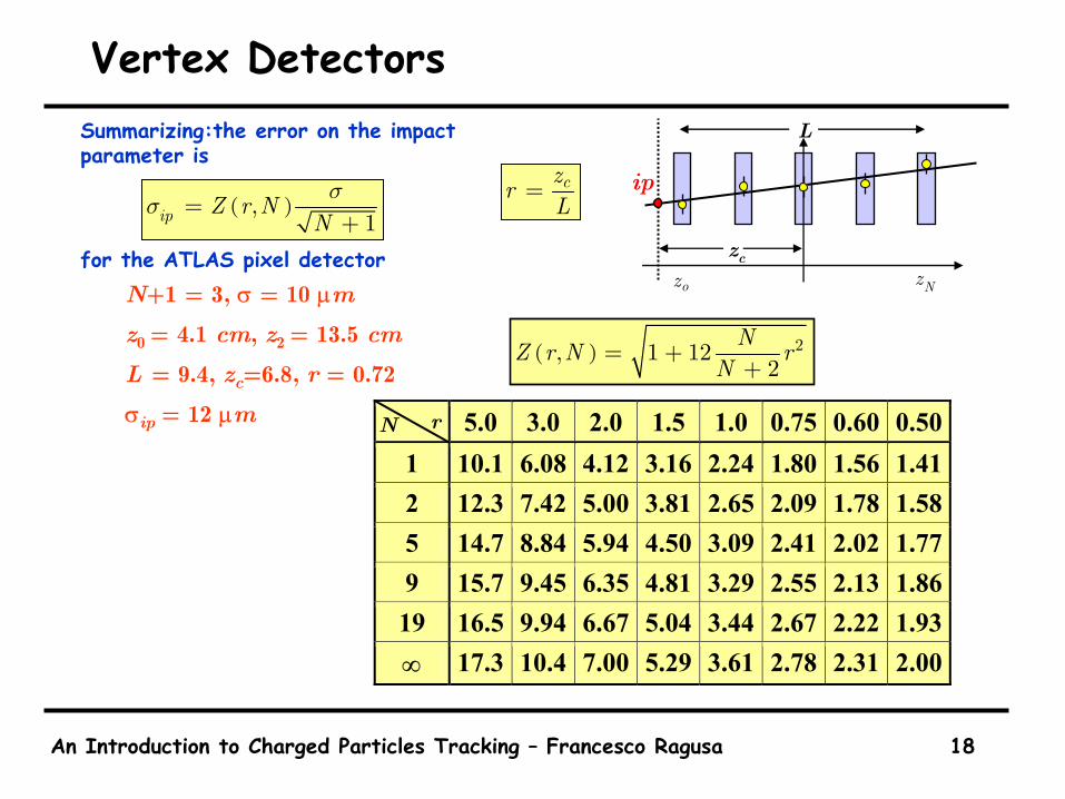
Vertex DetectorsSummarizing:the error on the impact parameter is

for the ATLAS pixel detectorN+1 = 3, σ = 10 µm

z0 = 4.1 cm, z2 = 13.5 cm

L = 9.4, zc=6.8, r = 0.72

σip = 12 µm

oz Nz

L

zc

ip( ),

1ip Z r NNσσ =+

( ) 2, 1 122

NZ r N rN

= ++

czrL

=

5.0 3.0 2.0 1.5 1.0 0.75 0.60 0.501 10.1 6.08 4.12 3.16 2.24 1.80 1.56 1.412 12.3 7.42 5.00 3.81 2.65 2.09 1.78 1.585 14.7 8.84 5.94 4.50 3.09 2.41 2.02 1.779 15.7 9.45 6.35 4.81 3.29 2.55 2.13 1.86

19 16.5 9.94 6.67 5.04 3.44 2.67 2.22 1.93∞ 17.3 10.4 7.00 5.29 3.61 2.78 2.31 2.00

N r


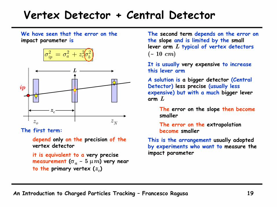
Vertex Detector + Central DetectorWe have seen that the error on the impact parameter is

The first term:depend only on the precision of the vertex detectorit is equivalent to a very precisemeasurement (σa ~ 5 µm) very nearto the primary vertex (zc)

The second term depends on the error on the slope and is limited by the small lever arm L typical of vertex detectors (~ 10 cm)It is usually very expensive to increase this lever armA solution is a bigger detector (Central Detector) less precise (usually less expensive) but with a much bigger lever arm L

The error on the slope then become smallerThe error on the extrapolationbecome smaller

This is the arrangement usually adoptedby experiments who want to measure the impact parameter

2 2 2 2a cip bzσ σ σ= +

L

zc

oz Nz

ip


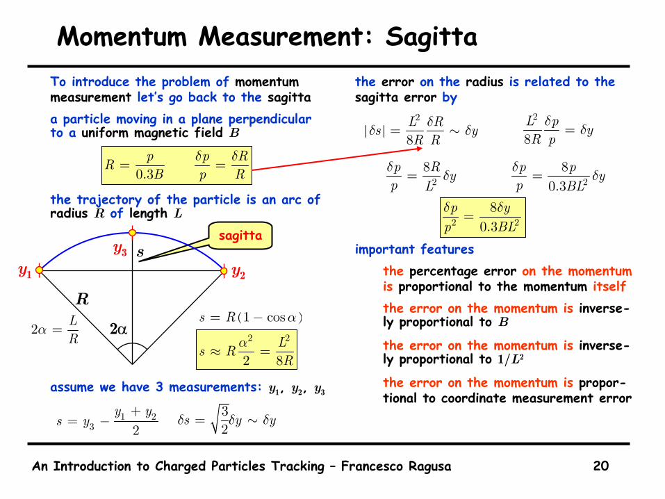
Momentum Measurement: SagittaTo introduce the problem of momentummeasurement let’s go back to the sagittaa particle moving in a plane perpendicular to a uniform magnetic field B

the trajectory of the particle is an arc of radius R of length L

assume we have 3 measurements: y1, y2, y3

the error on the radius is related to the sagitta error by

important featuresthe percentage error on the momentum is proportional to the momentum itselfthe error on the momentum is inverse-ly proportional to B

the error on the momentum is inverse-ly proportional to 1/L2

the error on the momentum is propor-tional to coordinate measurement error

2α

R

s

2 LR

α =( )1 coss R α= −

2 2

2 8Ls RR

α≈ =

sagitta

y1 y2

y3

0.3p p RRB p R

δ δ= =

1 23 2y y

s y+

= −32

s y yδ δ δ= ∼

2

8L Rs yR Rδδ δ= ∼

2

8L p yR pδ δ=

28p R y

p Lδ δ= 2

80.3

p p yp BLδ δ=

2 28

0.3p yp BLδ δ=


Tracking In Magnetic FieldThe previous example showed the basic features of momentum measurementLet’s now turn to a more complete trea-tement of the measurement of the char-ged particle trajectoryWe have already seen that for an homo-geneus magnetic field the trajectory projected on a plane perpendicular to the magnetic field is a circle

for not too low momenta we can use a linear approximation

we are led to the parabolic approximationof the trajectory

let’s stress that as far as the track pa-rameters is concerned the dependence is linearThe parameters a,b,c are

intercept at the originslope at the originradius of curvature (momentum)

( ) ( )2 2 2o oy y x x R− + − =

( )0a y=

0x

dybdx =

=

12

cR

= −

( )22o oy y R x x= + − −

( )221

2o

ox xy y RR

− ≈ + −

( ) 22

122

o oo

x xy y R x xR RR

= + − + −

2y a bx cx= + +

( )22 >> - oR x x


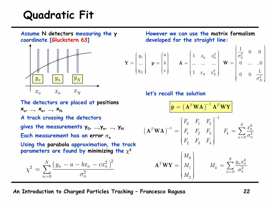
Quadratic FitAssume N detectors measuring the ycoordinate [Gluckstern 63]

The detectors are placed at positionsxo, …, xn, …, xN

A track crossing the detectorsgives the measurements y0, …,yn, …, yN

Each measurement has an error σn

Using the parabola approximation, the track parameters are found by minimizing the χ2

However we can use the matrix formalismdeveloped for the straight line:

let’s recall the solution

( )222

20

Nn n n

nn

y a bx cxχ

σ=

− − −= ∑

ox nx Nx

Nyoy ny

20 0

2

1... ... ...

1 N N

x x

x x

=

A

20

2

10 0

0 ... ..0

10 0N

σ

σ

=

W

a

bc

=

p...o

N

y

y

=

Y

( ) 1T T−=p A WA A WY

( )

10 1 2

11 2 3

2 3 4

T

F F F

F F F

F F F

−

−

=

A WA 20

N kn

knn

xFσ=

= ∑

0

1

2

T

M

M

M

=

A WY 20

N kn n

knn

y xMσ=

= ∑


Quadratic FitThe result is [4: Avery 1991, Blum-Rolandi 1993 p.204, Gluckstern 63]

The quantities Fij are the determinantsof the 2x2 matrices obtained from the 3x3 matrix F by removing row i, column j

The covariance matrix

The result can be found in [Blum-Rolandi, p. 206]To get some idea of the covariance matrix let’s first compute it by setting the origin at the center of the track

with this choice one can “easely” find

2n n n n n n

n n n n n

y G y G y Ga b c

G x G x G= = =∑ ∑ ∑

∑ ∑ ∑11 21 2 31

n n nG F x F x F= − +

12 22 2 32n n nP F x F x F= − + −

13 23 2 33n n nQ F x F x F= − +

( )

10 1 2

11 2 3

2 3 4

T

F F F

F F F

F F F

−

−

= =

pV A WA

0 1

Nn

cn

xxN=

=+∑

( )( )

( )( )( )

( )( ) ( )( )

1 3

0 2

2

2 2

24

4 2 3

242

0 4 2 4 3

0

1

1 2121 2 3 6 4

2401 1 2 3

180

F F

NF

L N NF

NN N N NLF

NL N N N NS F F F

N

σ

σ

σ

σ

= =

+=

+ +=

+ + + −=

− + + += − =


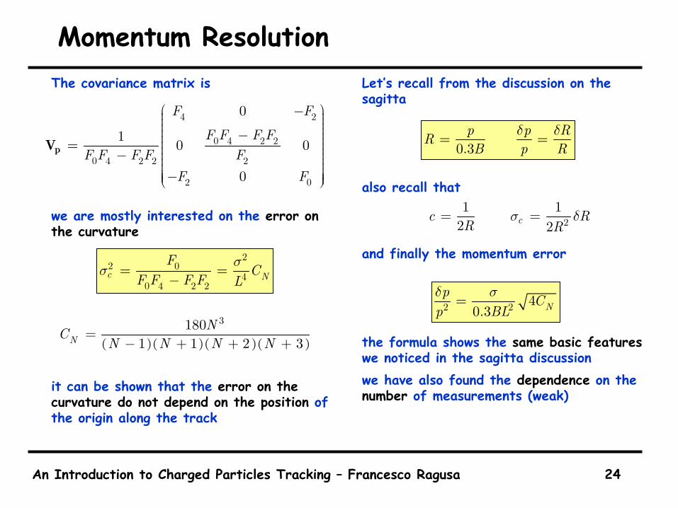
Momentum ResolutionThe covariance matrix is

we are mostly interested on the error on the curvature

it can be shown that the error on the curvature do not depend on the position of the origin along the track

Let’s recall from the discussion on the sagitta

also recall that

and finally the momentum error

the formula shows the same basic featureswe noticed in the sagitta discussionwe have also found the dependence on the number of measurements (weak)

4 2

0 4 2 2

0 4 2 2 2

02

0

1 0 0

0

F F

F F F FF F F F F

F F

− − = − −

pV

22 0

40 4 2 2

c NF

CF F F F L

σσ = =−

( )( )( )( )

31801 1 2 3N

NCN N N N

=− + + +

0.3p p RRB p R

δ δ= =

12

cR

= 21

2c RR

σ δ=

2 2 40.3 N

p Cp BLδ σ=


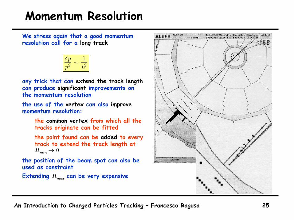
Momentum ResolutionWe stress again that a good momentum resolution call for a long track

any trick that can extend the track lengthcan produce significant improvements on the momentum resolutionthe use of the vertex can also improvemomentum resolution:

the common vertex from which all the tracks originate can be fittedthe point found can be added to every track to extend the track length at Rmin → 0

the position of the beam spot can also be used as constraintExtending Rmax can be very expensive

2 21p

p Lδ ∼


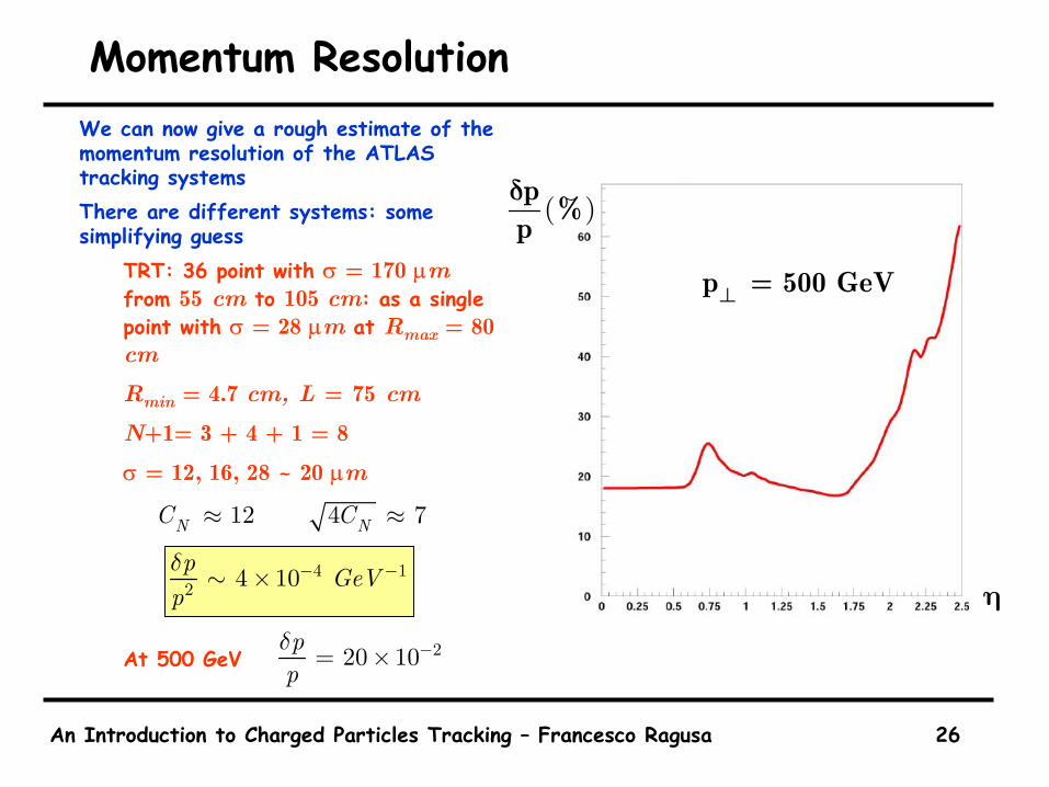
Momentum ResolutionWe can now give a rough estimate of the momentum resolution of the ATLAS tracking systemsThere are different systems: some simplifying guess

TRT: 36 point with σ = 170 µmfrom 55 cm to 105 cm: as a single point with σ = 28 µm at Rmax = 80 cm

Rmin = 4.7 cm, L = 75 cm

N+1= 3 + 4 + 1 = 8

σ = 12, 16, 28 ~ 20 µm

At 500 GeV

12 4 7N NC C≈ ≈

η

( )p %pδ

p = 500 GeV⊥

4 12 4 10p GeVpδ − −×∼

220 10ppδ −= ×


Momentum Resolution


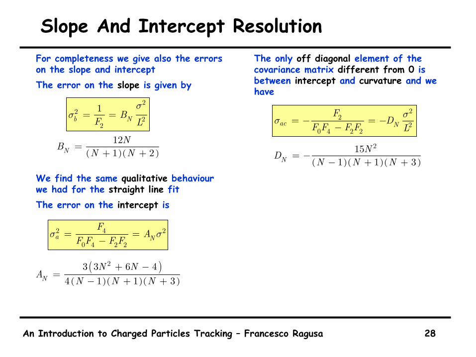
Slope And Intercept ResolutionFor completeness we give also the errors on the slope and interceptThe error on the slope is given by

We find the same qualitative behaviour we had for the straight line fitThe error on the intercept is

The only off diagonal element of the covariance matrix different from 0 is between intercept and curvature and we have

22

22

1b NBF L

σσ = =

2 4 2

0 4 2 2a N

FA

F F F Fσ σ= =

−

( )( )( )

2151 1 3N

NDN N N

= −− + +

( )( )121 2NNB

N N=

+ +

( )( )( )( )

23 3 6 44 1 1 3N

N NA

N N N+ −

=− + +

22

20 4 2 2

ac NF

DF F F F L

σσ = − = −−


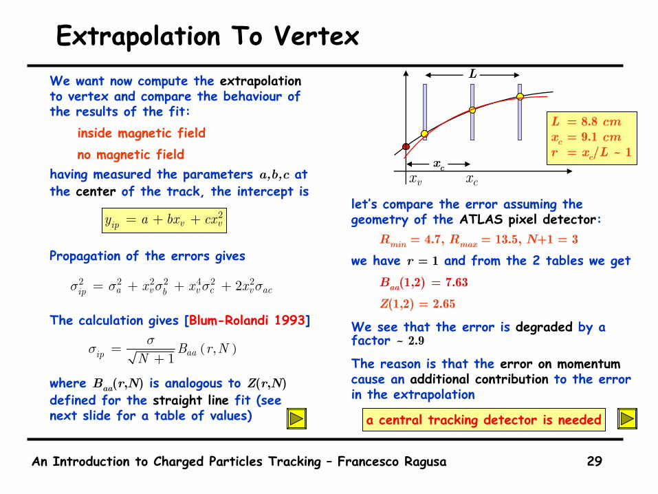
Extrapolation To VertexWe want now compute the extrapolationto vertex and compare the behaviour of the results of the fit:

inside magnetic fieldno magnetic field

having measured the parameters a,b,c at the center of the track, the intercept is

Propagation of the errors gives

The calculation gives [Blum-Rolandi 1993]

where Baa(r,N) is analogous to Z(r,N)defined for the straight line fit (see next slide for a table of values)

let’s compare the error assuming the geometry of the ATLAS pixel detector:

Rmin = 4.7, Rmax = 13.5, N+1 = 3

we have r = 1 and from the 2 tables we getBaa(1,2) = 7.63Z(1,2) = 2.65

We see that the error is degraded by a factor ~ 2.9

The reason is that the error on momentumcause an additional contribution to the error in the extrapolation

2v vipy a bx cx= + +

2 2 2 2 4 2 22a v v c v acip bx x xσ σ σ σ σ= + + +

vx cx

L

xc

( ),1 aaip B r N

Nσσ =+

a central tracking detector is needed

L = 8.8 cmxc = 9.1 cmr = xc/L ~ 1


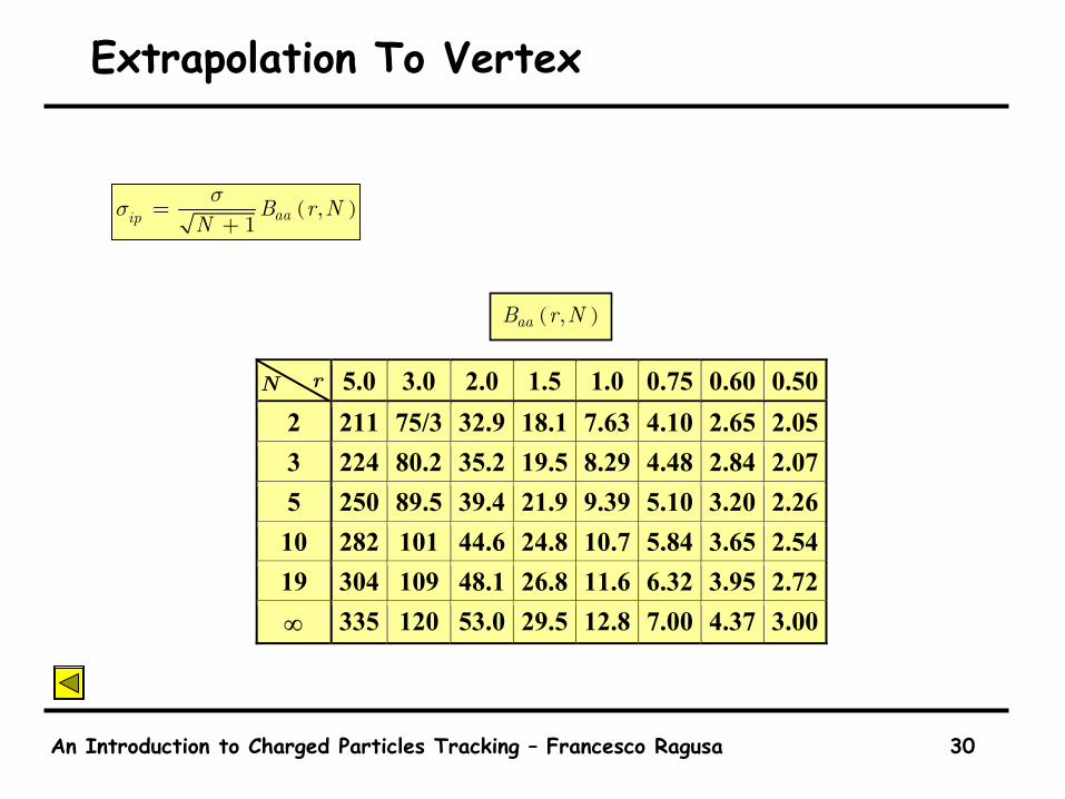
Extrapolation To Vertex

( ),1 aaip B r N

Nσσ =+

( ),aaB r N

5.0 3.0 2.0 1.5 1.0 0.75 0.60 0.502 211 75/3 32.9 18.1 7.63 4.10 2.65 2.053 224 80.2 35.2 19.5 8.29 4.48 2.84 2.075 250 89.5 39.4 21.9 9.39 5.10 3.20 2.26

10 282 101 44.6 24.8 10.7 5.84 3.65 2.5419 304 109 48.1 26.8 11.6 6.32 3.95 2.72∞ 335 120 53.0 29.5 12.8 7.00 4.37 3.00

N r


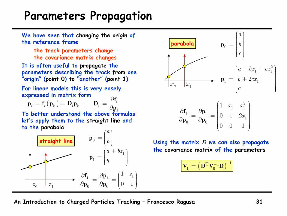
Parameters PropagationWe have seen that changing the origin of the reference frame

the track parameters changethe covariance matrix changes

It is often useful to propagate the parameters describing the track from one “origin” (point 0) to “another” (point 1)For linear models this is very easely expressed in matrix form

To better understand the above formulas let’s apply them to the straight line and to the parabola

Using the matrix D we can also propagate the covariance matrix of the parameters

0

a

b =

p

( )i i ik k= =p f p D p

11 1

0 0

1

0 1

z ∂ ∂ = = ∂ ∂

f pp p

21 1

1 11

0 0

1

0 1 2

0 0 1

x x

x

∂ ∂ = = ∂ ∂

f pp p

ii

k

∂=

∂f

Dp

ox 1x

oz 1z

11

a bz

b

+ = p

straight line

parabola 0

a

bc

=

p

21 1

1 12

a bx cx

b cxc

+ + = +

p

( ) 1T 101

−−=V D V D


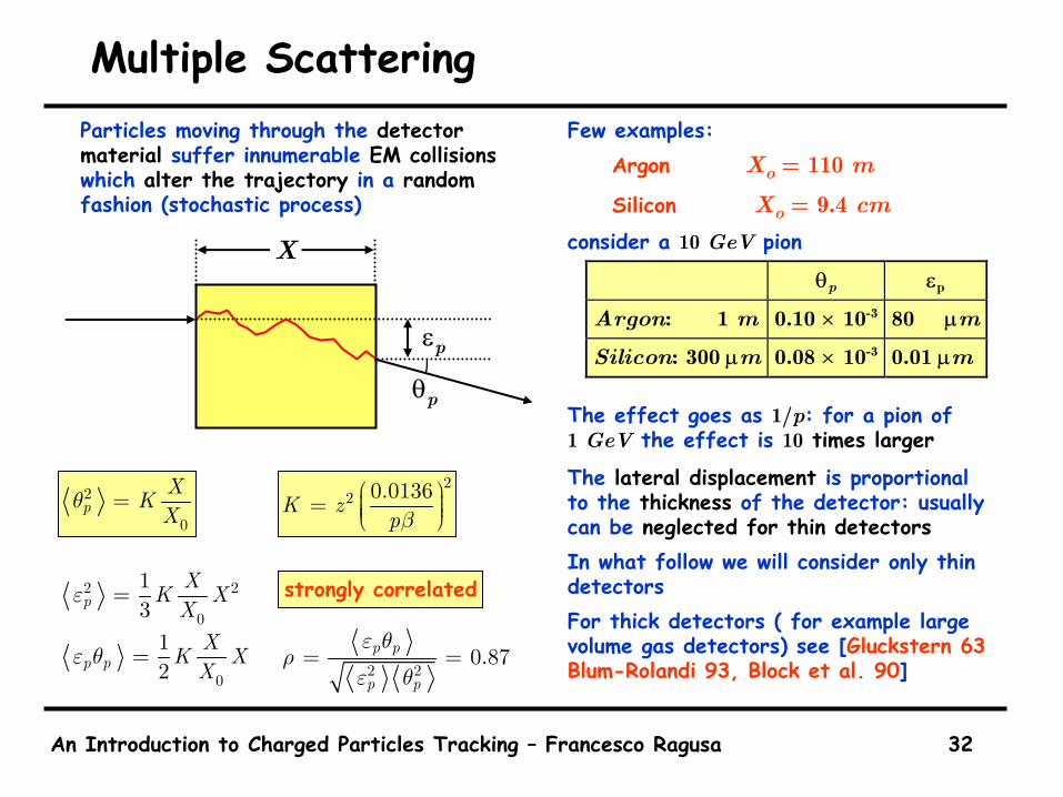
Multiple ScatteringParticles moving through the detector material suffer innumerable EM collisionswhich alter the trajectory in a randomfashion (stochastic process)

Few examples:Argon Xo = 110 m

Silicon Xo = 9.4 cmconsider a 10 GeV pion

The effect goes as 1/p: for a pion of 1 GeV the effect is 10 times larger

The lateral displacement is proportional to the thickness of the detector: usually can be neglected for thin detectorsIn what follow we will consider only thin detectorsFor thick detectors ( for example large volume gas detectors) see [Gluckstern 63 Blum-Rolandi 93, Block et al. 90]

X

εp

θp

22 0.0136K zpβ

= 2

0p

XKX

θ =

2 20.87p p

p p

ε θρ

ε θ= =

θp εp

Argon: 1 m 0.10 × 10-3 80 µm

Silicon: 300 µm 0.08 × 10-3 0.01 µm

0

12p pXK XX

ε θ =

2 2

0

13pXK XX

ε = strongly correlated


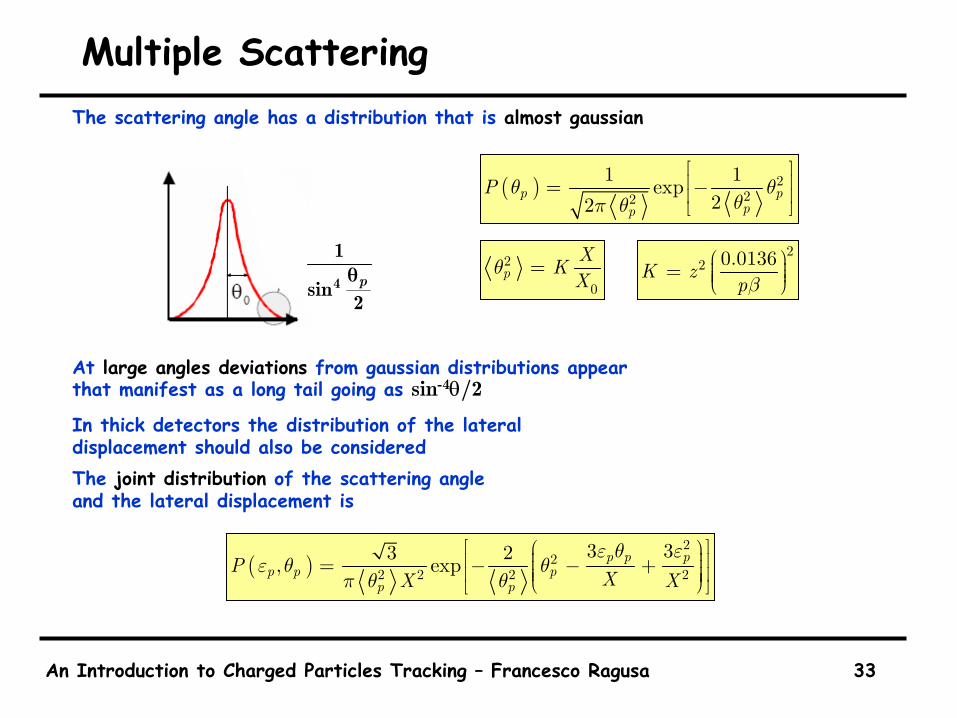
Multiple ScatteringThe scattering angle has a distribution that is almost gaussian

At large angles deviations from gaussian distributions appear that manifest as a long tail going as sin-4θ/2In thick detectors the distribution of the lateral displacement should also be consideredThe joint distribution of the scattering angle and the lateral displacement is

( )2

22 2 2 2

3 33 2, exp p p pp p p

p pP

XX Xε θ ε

ε θ θπ θ θ

= − − +

( ) 222

1 1exp22

p ppp

P θ θθπ θ

= −

4

1

sin 2θp

22 0.0136K zpβ

= 2

0p

XKX

θ =


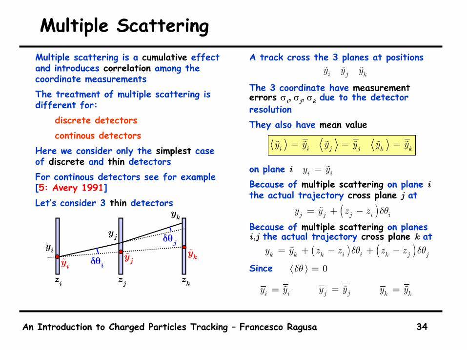
Multiple ScatteringMultiple scattering is a cumulative effect and introduces correlation among the coordinate measurementsThe treatment of multiple scattering is different for:

discrete detectorscontinous detectors

Here we consider only the simplest case of discrete and thin detectorsFor continous detectors see for example [5: Avery 1991]Let’s consider 3 thin detectors

A track cross the 3 planes at positions

The 3 coordinate have measurement errors σi, σj, σk due to the detector resolutionThey also have mean value

on plane iBecause of multiple scattering on plane i the actual trajectory cross plane j at

Because of multiple scattering on planes i,j the actual trajectory cross plane k at

Since

( )j j j i iy y z z δθ= + −

( ) ( )i i j jk k k ky y z z z zδθ δθ= + − + −

i j ky y y

i i j j k ky y y y y y= = =

i iy y=

0δθ =

j jy y= k ky y=i iy y=

iy jy ky

iz jz kz

iyjy

ky

iδθ

jδθ


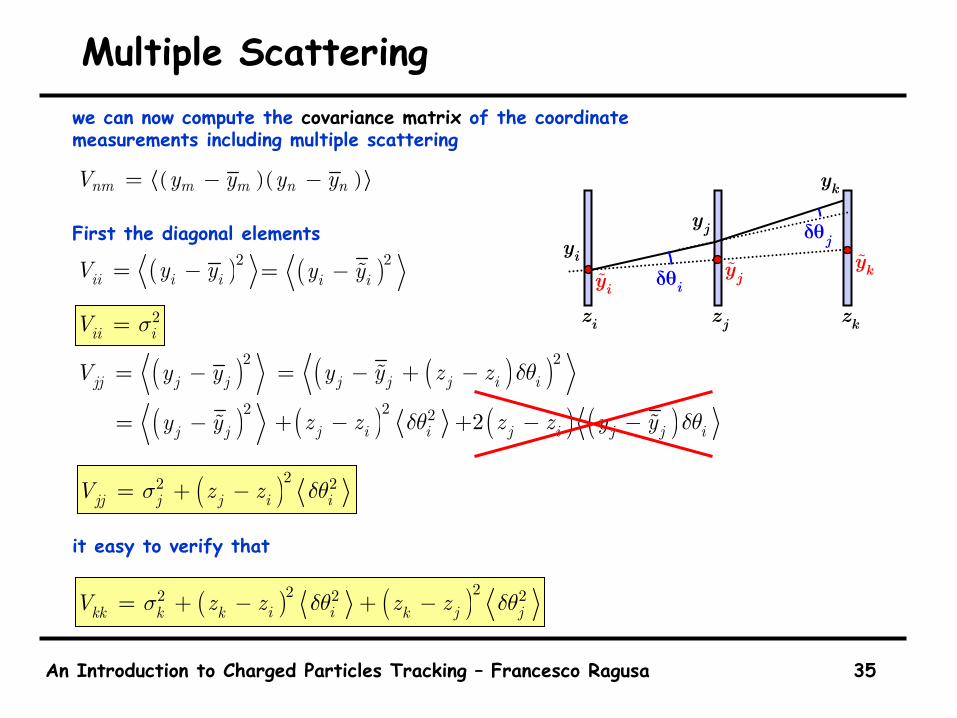
Multiple Scatteringwe can now compute the covariance matrix of the coordinate measurements including multiple scattering

First the diagonal elements

it easy to verify that

( )( )nm m m n nV y y y y= − −

( )2ii i iV y y= −

( ) ( )222 2 2i i j jkk k k kV z z z zσ δθ δθ= + − + −

( )2i iy y= −

2ii iV σ=

( )2jj j jV y y= − ( )( )2j j j i iy y z z δθ= − + −

( )2j jy y= − ( )2 2j i iz z δθ+ − ( ) ( )2 j i j j iz z y y δθ+ − −

( )22 2jj j j i iV z zσ δθ= + −

iy jy ky

iz jz kz

iyjy

ky

iδθ

jδθ


Multiple Scattering

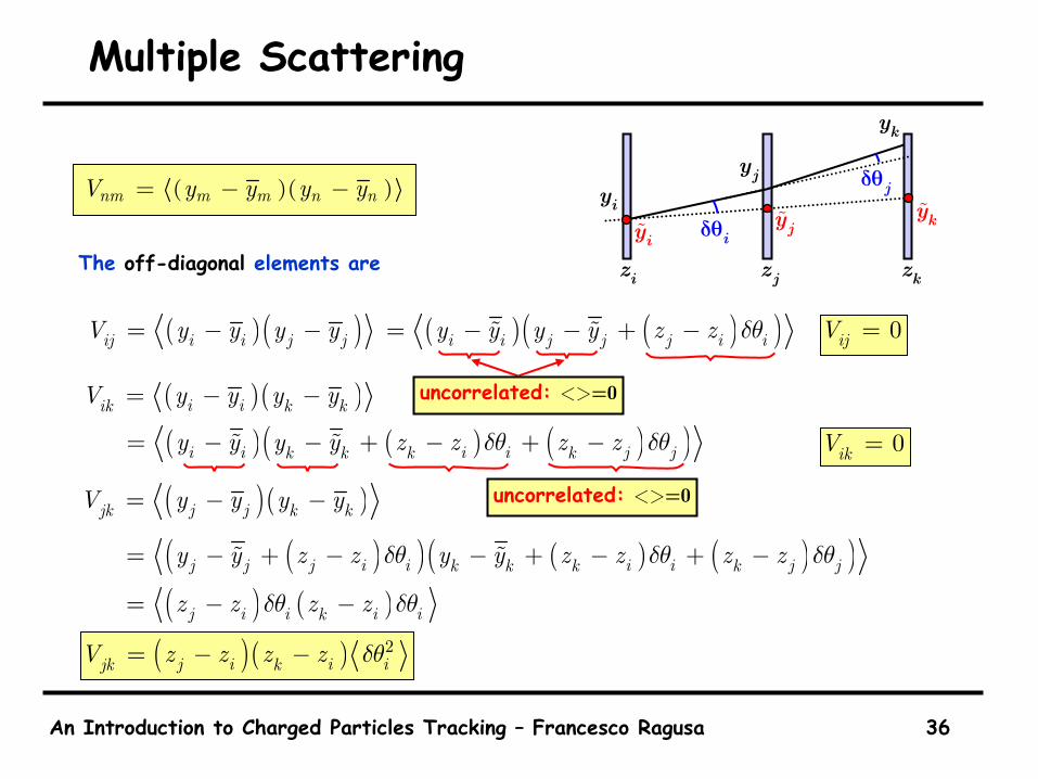
The off-diagonal elements are

( )( )nm m m n nV y y y y= − −

( )( )ij i i j jV y y y y= − − ( ) ( )( )i i j j j i iy y y y z z δθ= − − + − 0ijV =

( )( )i iik k kV y y y y= − −

( ) ( ) ( )( )i i i i j jk k k ky y y y z z z zδθ δθ= − − + − + − 0ikV =

( )( )j jjk k kV y y y y= − −

( )( ) ( ) ( )( )j j j i i i i j jk k k ky y z z y y z z z zδθ δθ δθ= − + − − + − + −

( ) ( )j i i i ikz z z zδθ δθ= − −

( )( ) 2j i i ijk kV z z z z δθ= − −

iy jy ky

iz jz kz

iyjy

ky

iδθ

jδθ

uncorrelated: <>=0

uncorrelated: <>=0


Multiple ScatteringSummarizing, the covariance matrix is

The second matrix hasdiagonal elements due to any previous material affectingthe trajectory impact point at the given planeoff diagonal elements: only presents if a previous material layeraffects at the same time the trajectory impact points for the 2 planes

the same scattering at plane iaffects the trajectory at plane j and plane k

( ) ( )( )( )( ) ( ) ( )

2

22 2 2

2 222 2 2

0 0 00 0

0 0 0

0 0 0

i

j j i i i j i ik

k i j i i i i j i jk k

V z z z z z z

z z z z z z z z

σ

σ δθ δθ

σ δθ δθ δθ

= + − − − − − − + −

iy jy ky

iz jz kz

iyjy

ky

iδθ

jδθ


Track Fit With Multiple ScatteringThe methods developed to fit a track to the measured points can be used to perform a fit taking into account M.S.

the covariance matrix is computedthe same fit procedure is applied

Let’s now try to understand qualitativelythe effect of multiple scattering on the determination of tracks parameters:

the size of the effect goes as 1/pthen the effect is important for low momentum track

Assume we are dominated by multiple scattering

the momentum resolution is given by

the coordinate error due to M.S. is

we have then

We conclude:for low momentum the percentage momentum resolution reach a almost constant value (still dependent on β)

The momentum resolution only improves as 1/L

The additional factor 1/N can help but in this case uniform spacing is essential2 2 4

0.3 Np

Ap BLδ σ=

0.0136o

L L XN N p X

σ δθβ

=∼

ppδ → constant

0

40.0136 10.3

NAp Xp X BL Nδ

β∼


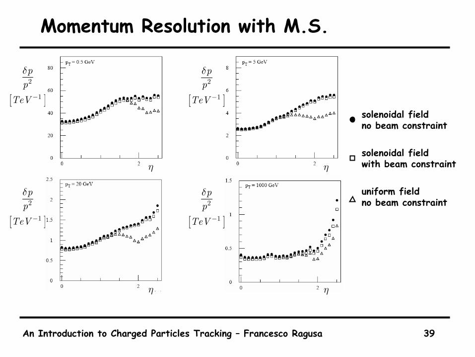
Momentum Resolution with M.S.

solenoidal fieldno beam constraint

solenoidal fieldwith beam constraint

uniform fieldno beam constraint

[ ]2

1

pp

TeV

δ

−

[ ]2

1

pp

TeV

δ

−

[ ]2

1

pp

TeV

δ

−

[ ]2

1

pp

TeV

δ

−

η

η

η

η


Track Fit With Multiple ScatteringSame kind of considerations for the error on the slope and on the interceptthe multiple scattering error is

the error on the slope is

we cannot improve anymore the error on the slope (direction) by increasing the lever arm

the limit is set by the multiple scattering angle itself

As far as the impact parameterresolution

large lever arm degrade the impact parameter resolution

for a given error on the slope set by the multiple scattering angle the error on the extrapolation goes as the lever arm

Unfortunately both ATLAS and CMS have a lot of material

silicon detectors for high precisionsilicon for radiation hardnesssilicon for rate capabilities

( ),1 aaip B r N

Nσσ =+

b NB L

σσ =

0.0136o

L L XN N p X

σ δθβ

=∼

0.0136b N

o

L XBLN p X

σβ

=

0.0136Nb

o

B XN p X

σβ

=

( ), 0.01361

aaip

o

B r N L XN p XN

σβ

=+


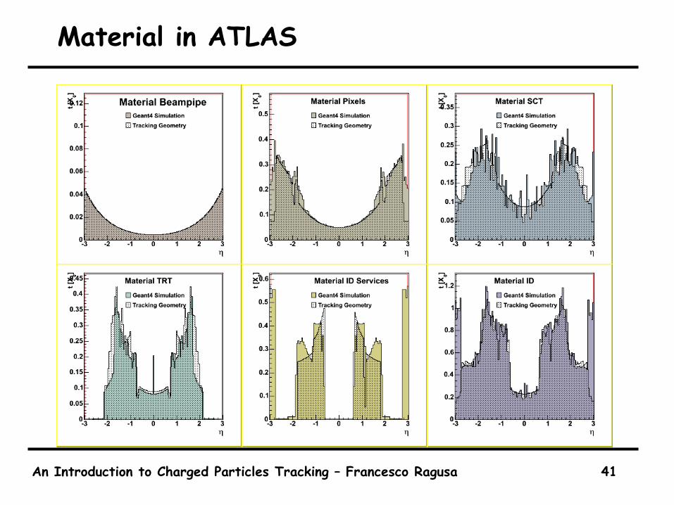
Material in ATLAS


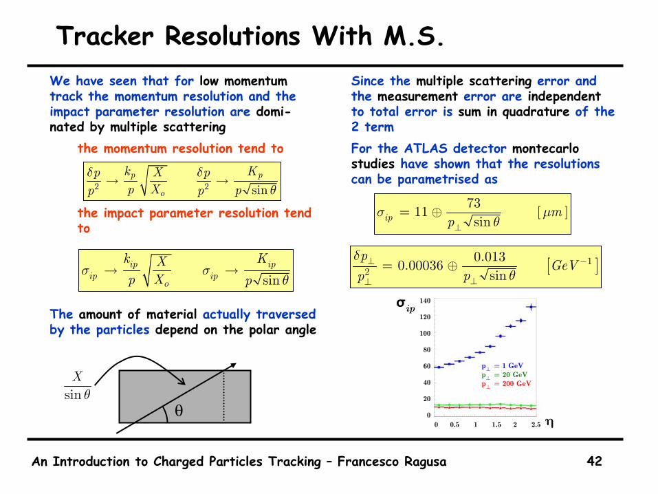
Tracker Resolutions With M.S.We have seen that for low momentumtrack the momentum resolution and the impact parameter resolution are domi-nated by multiple scattering

the momentum resolution tend to

the impact parameter resolution tend to

The amount of material actually traversed by the particles depend on the polar angle

Since the multiple scattering error and the measurement error are independentto total error is sum in quadrature of the 2 termFor the ATLAS detector montecarlostudies have shown that the resolutions can be parametrised as

θsinXθ

2p

o

kp Xp Xp

δ →

ipip

o

k Xp X

σ → [ ]12

0.0130.00036sin

pGeV

ppδ

θ⊥ −

⊥⊥= ⊕

[ ]7311sinip m

pσ µ

θ⊥= ⊕

σip

η0 0.5 1 1.5 2 2.5

140

120

100

80

60

40

20

0

p = 20 GeVp

p = 1 GeV

= 200 GeV⊥⊥⊥

2 2 sinp p

o

k Kp X pp X pp p

δ δθ

→ →

sinip ip

ip ipo

k KXp X p

σ σθ

→ →


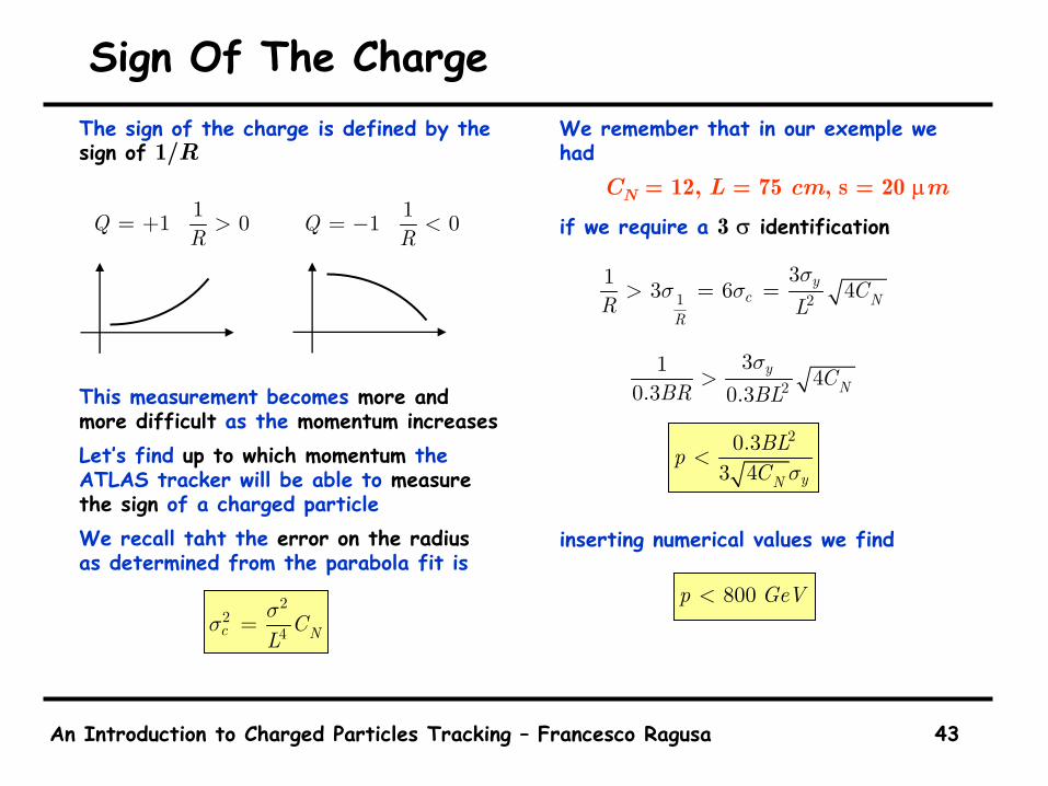
Sign Of The ChargeThe sign of the charge is defined by the sign of 1/R

This measurement becomes more and more difficult as the momentum increasesLet’s find up to which momentum the ATLAS tracker will be able to measure the sign of a charged particleWe recall taht the error on the radiusas determined from the parabola fit is

We remember that in our exemple we had

CN = 12, L = 75 cm, s = 20 µm

if we require a 3 σ identification

inserting numerical values we find

11 0QR

= + > 11 0QR

= − <

22

4c NCLσσ =

1 231 3 6 4y

c NR

CR L

σσ σ> = =

231 4

0.3 0.3y

NCBR BLσ

>

20.33 4 yN

BLpC σ

<

800p GeV<


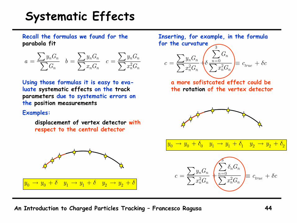
Systematic EffectsRecall the formulas we found for the parabola fit

Using those formulas it is easy to eva-luate systematic effects on the trackparameters due to systematic errors on the position measurementsExamples:

displacement of vertex detector with respect to the central detector

Inserting, for example, in the formula for the curvature

a more sofistcated effect could be the rotation of the vertex detector

2n n n n n n

n n n n n

y G y G y Ga b c

G x G x G= = =∑ ∑ ∑

∑ ∑ ∑

0 0 1 1 2 2y y y y y yδ δ δ→ + → + → +

2n n

n n

y Gc

x G= ∑∑

3

02

nn

n n

G

x Gδ =+∑∑ truec cδ≡ +

0 0 0 1 1 1 2 2 2y y y y y yδ δ δ→ + → + → +

2n n

n n

y Gc

x G= ∑∑

3

02

n nn

n n

G

x G

δ=+∑∑ truec cδ≡ +


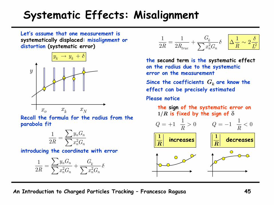
Systematic Effects: MisalignmentLet’s assume that one measurement is systematically displaced: misalignment or distortion (systematic error)

Recall the formula for the radius from the parabola fit

introducing the coordinate with error

the second term is the systematic effecton the radius due to the systematic error on the measurementSince the coefficients Gk are know the effect can be precisely estimatedPlease notice

the sign of the systematic error on 1/R is fixed by the sign of δ

k ky y δ→ +

ox kx Nx

y

21

2n n

n n

y GR x G= ∑∑

2 21

2n n k

n n n n

y G GR x G x G

δ= +∑∑ ∑

21 1

2 2k

n ntrue

GR R x G

δ= +∑

11 0QR

= + > 11 0QR

= − <

1 increasesR

1 decreasesR

21 2R L

δ∆ ∼


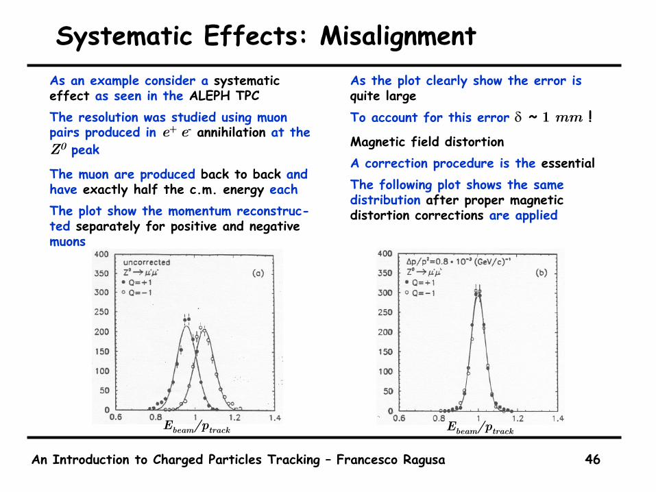
Systematic Effects: MisalignmentAs an example consider a systematic effect as seen in the ALEPH TPCThe resolution was studied using muon pairs produced in e+ e- annihilation at the Z0 peak

The muon are produced back to back and have exactly half the c.m. energy eachThe plot show the momentum reconstruc-ted separately for positive and negativemuons

As the plot clearly show the error is quite largeTo account for this error δ ~ 1 mm !Magnetic field distortionA correction procedure is the essentialThe following plot shows the same distribution after proper magnetic distortion corrections are applied

Ebeam/ptrack Ebeam/ptrack


Problems With The Fit ProcedureWe have learned how to use linear models to fit the projection of the charged particle trackThe method could be extendend to non linear problems (inhomogeneous magnetic field) by linearization and iterationThe solution of the problem is given by

to solve the problem the matrix Vhas to be invertedeasy if V diagonal ( time O(n) )

We have seen that multiple scatteringintroduces correlation among measure-ments and makes V non diagonal

For large detectors the dimension of Vcan be prohibitively large (time O(n3))The fit is normally used to rank track candidates during pattern recognition

The fit procedure gives the track parameters at a given surface or plane

Often prediction of the track crossing point at a different plane is needed

impact parametermatch with calorimetersmatch with particle ID (RICH)

The fit procedure described is not optimal for this problem:

multiple scattering makes prediction(extrapolation) non optimal

( ) 1T T−= = -1p A WA A WY W V


Kalman Filter

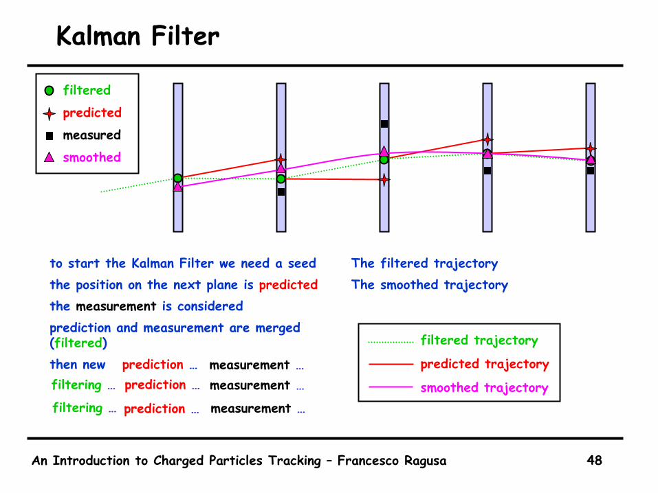
to start the Kalman Filter we need a seedthe position on the next plane is predictedthe measurement is consideredprediction and measurement are merged (filtered)then new prediction …

The filtered trajectoryThe smoothed trajectory

measurement …filtering … prediction … measurement …

filtering … prediction … measurement …

smoothed

filtered

predicted

measured

smoothed trajectory

filtered trajectory

predicted trajectory


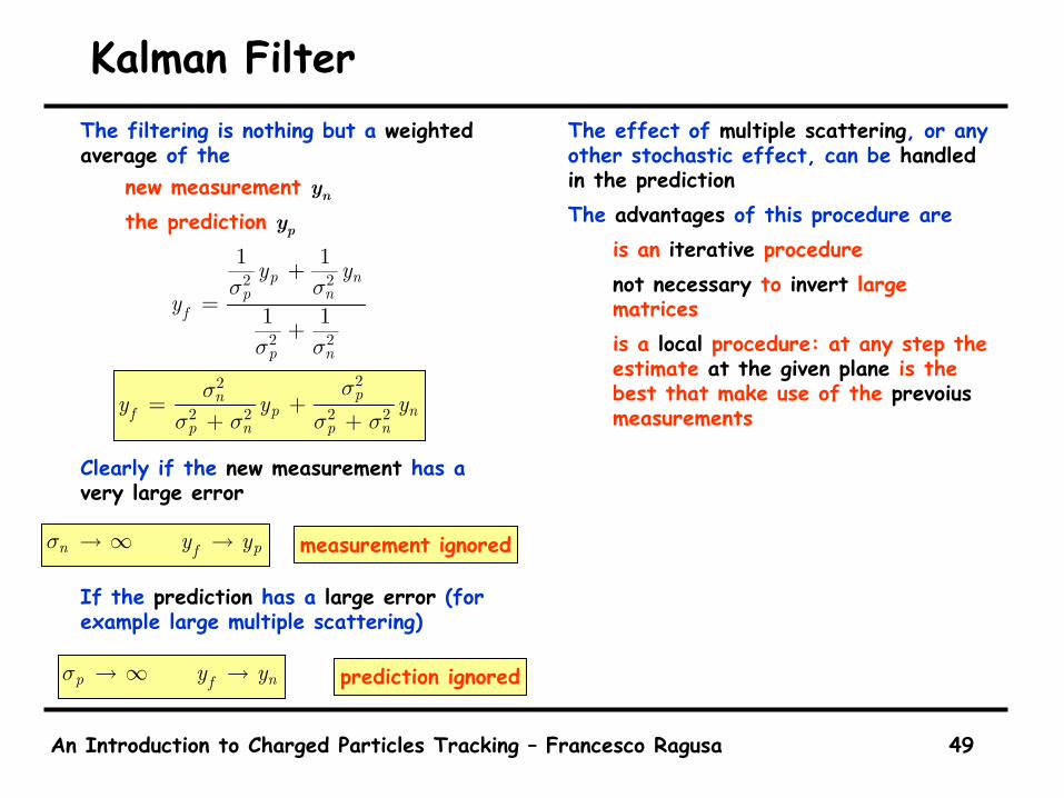
Kalman FilterThe filtering is nothing but a weightedaverage of the

new measurement yn

the prediction yp

Clearly if the new measurement has a very large error

If the prediction has a large error (for example large multiple scattering)

The effect of multiple scattering, or any other stochastic effect, can be handled in the predictionThe advantages of this procedure are

is an iterative procedurenot necessary to invert large matricesis a local procedure: at any step the estimate at the given plane is the best that make use of the prevoiusmeasurements

2 2

2 2

1 1

1 1

p np n

f

p n

y yy

σ σ

σ σ

+=

+

22

2 2 2 2pn

p nfp n p n

y y yσσ

σ σ σ σ= +

+ +

n pfy yσ → ∞ →

p nfy yσ → ∞ →

measurement ignored

prediction ignored


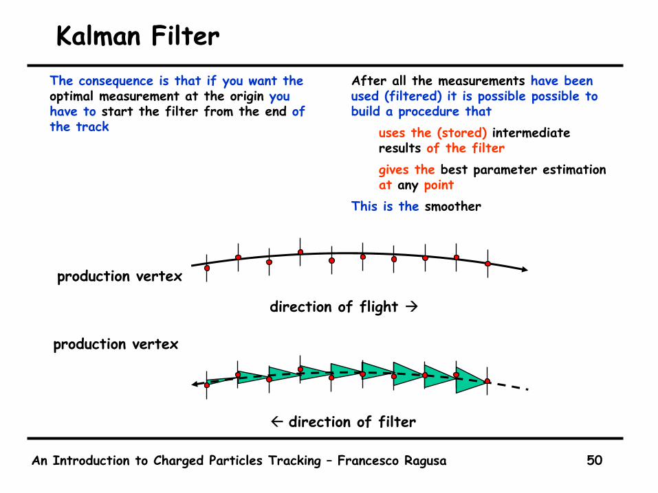
Kalman FilterThe consequence is that if you want the optimal measurement at the origin you have to start the filter from the end of the track

After all the measurements have been used (filtered) it is possible possible to build a procedure that

uses the (stored) intermediateresults of the filter gives the best parameter estimationat any point

This is the smoother

production vertex

direction of flight

direction of filter

production vertex


Kalman FilterApplications of Kalman Filter:

navigationradar trackingsonar rangingsatellite orbit computationstock prize prediction

It is used in all sort of fieldsEagle landed on the moon using KFGyroscopes in airplanes use KF

Usually the problem is to estimate a state of some sort and its uncertainty

location and velocity of airplanetrack parameters of charged particles in HEP experiments

However we do not observe the state directly

We only observe some measurementsfrom sensors which are noisy:

radar trackingcharged particle tracking detectors

As an additional complication the state evolve in time with is own uncertainties: process stochastic noise

deviation from trajectory due to random windmultiple scattering

In case of tracking in HEP instead of time we can consider the evolution of the track parameter at the discrete layerswhere the detectors perform the measurement


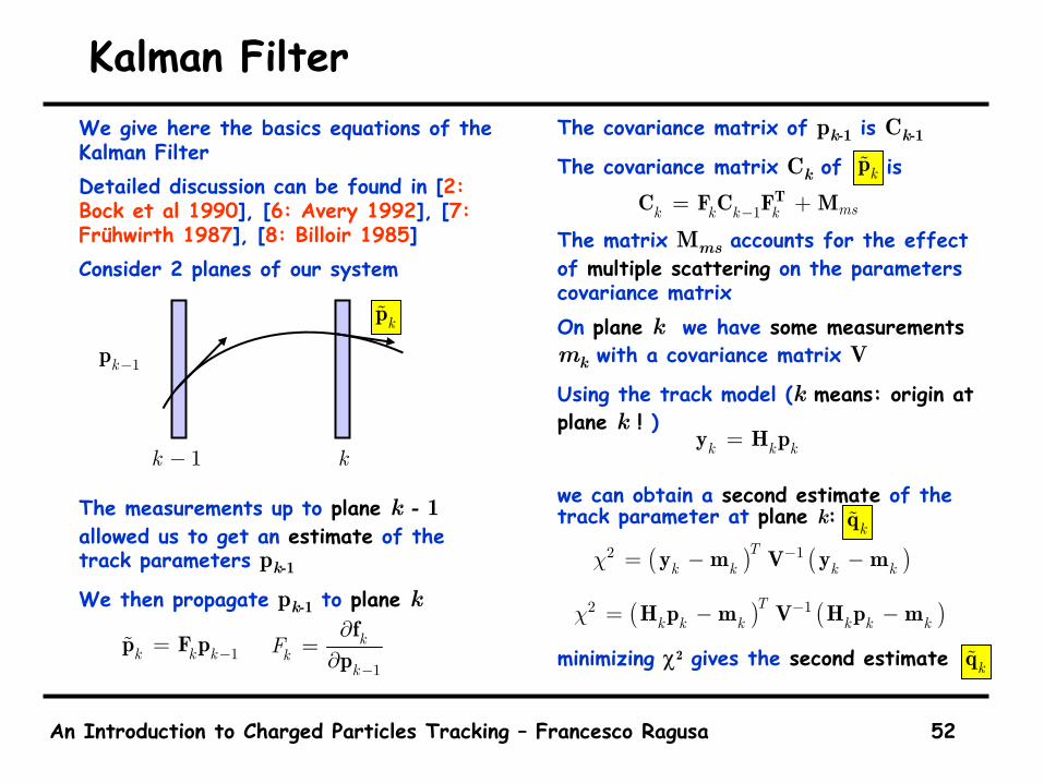
Kalman FilterWe give here the basics equations of the Kalman FilterDetailed discussion can be found in [2: Bock et al 1990], [6: Avery 1992], [7: Frühwirth 1987], [8: Billoir 1985]Consider 2 planes of our system

The measurements up to plane k - 1allowed us to get an estimate of the track parameters pk-1

We then propagate pk-1 to plane k

1k − k

1k−pkp

1

kk

kF

−

∂=

∂f

p1k k k−=p F p

1 msk k k k−= +TC F C F M

k k k=y H p

kp

( ) ( )2 1Tk k k kχ −= − −y m V y m

( ) ( )2 1Tk k k k k kχ −= − −H p m V H p m

kq

The covariance matrix of pk-1 is Ck-1

The covariance matrix Ck of is

The matrix Mms accounts for the effect of multiple scattering on the parameters covariance matrixOn plane k we have some measurementsmk with a covariance matrix V

Using the track model (k means: origin at plane k ! )

we can obtain a second estimate of the track parameter at plane k:

minimizing χ2 gives the second estimate kq


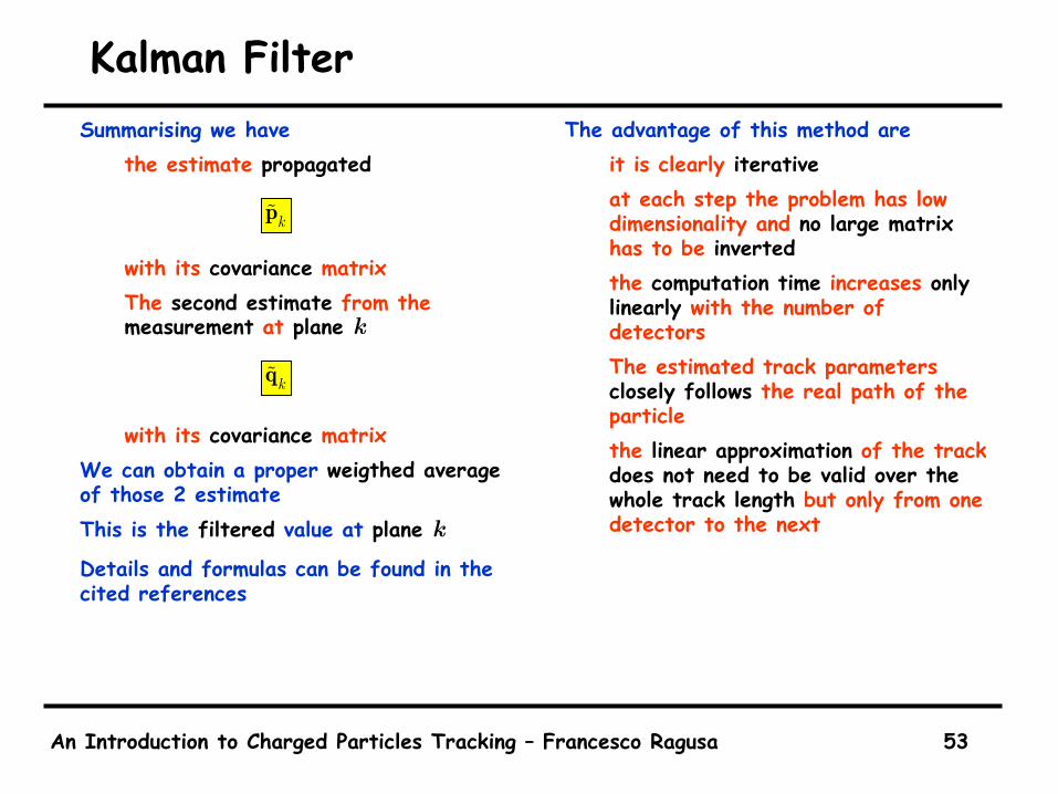
Kalman FilterSummarising we have

the estimate propagated

with its covariance matrixThe second estimate from the measurement at plane k

with its covariance matrixWe can obtain a proper weigthed averageof those 2 estimateThis is the filtered value at plane kDetails and formulas can be found in the cited references

The advantage of this method areit is clearly iterativeat each step the problem has low dimensionality and no large matrixhas to be invertedthe computation time increases onlylinearly with the number of detectorsThe estimated track parameters closely follows the real path of the particlethe linear approximation of the track does not need to be valid over the whole track length but only from one detector to the next

kp

kq


ConclusionsWe have seen the basic aspects of tracking with and without magnetic fieldsIn both cases we have shown the use of powerful and easy linear modelsWe have discussed optimization of

momentum resulution: track lengthimpact parameter resolution: vertex detector + central detector

We have discussed the importance of multiple scattering at low momentumWe have introduced the Kalman Filter

a powerful iterative technique to optimally solve the tracking problem

I Hope It Is Rather A Beginning

I hope you found tracking interesting and

that soon some of you will work on the tracking

detector of his/her experiment


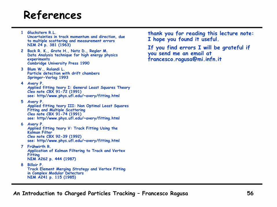
References1 Gluckstern R.L.

Uncertainties in track momentum and direction, dueto multiple scattering and measurement errorsNIM 24 p. 381 (1963)

2 Bock R. K., Grote H., Notz D., Regler M.Data Analysis technique for high energy physicsexperimentsCambridge University Press 1990

3 Blum W., Rolandi L.Particle detection with drift chambersSpringer-Verlag 1993

4 Avery P.Applied fitting teory I: General Least Squares TheoryCleo note CBX 91-72 (1991)see: http//www.phys.ufl.edu/~avery/fitting.html

5 Avery P.Applied fitting teory III: Non Optimal Least SquaresFitting and Multiple ScatteringCleo note CBX 91-74 (1991)see: http//www.phys.ufl.edu/~avery/fitting.html

6 Avery P.Applied fitting teory V: Track Fitting Using the Kalman FilterCleo note CBX 92-39 (1992)see: http//www.phys.ufl.edu/~avery/fitting.html

7 Frühwirth R.Application of Kalman Filtering to Track and VertexFittingNIM A262 p. 444 (1987)

8 Billoir P.Track Element Merging Strategy and Vertex Fittingin Complex Modular DetectorsNIM A241 p. 115 (1985)

thank you for reading this lecture note: I hope you found it useful.If you find errors I will be grateful if you send me an email [email protected]

Documents

An Introduction to Charged Particles Trackingphysics.iitm.ac.in/~sercehep2013/track2_Gagan_Mohanty.pdf · An Introduction to Charged Particles Tracking – Francesco Ragusa 4 Magnetic