1

Charged Particles Moving in an Magnetic Field

Equipment for Part 1 Qty Item Parts Number

1 Magnetic Field Sensor CI-6520A

1 Zero Gauss Chamber EM-8652

1 Dip Needle SF-8619

1 Angle Indicator ME-9495

1 Universal Table Clamp ME-9376B

1 Large Rod ME-8736

1 Adjustable Angle Clamp ME-8744

Equipment for Part 2Qty Equipment Parts Number

1 e/m Apparatus SE-9629

1 High Voltage Power Supply SF-9585A

2 Low Voltage Power Supply SF-9584B

8 Patch Cords

1 Multimeter

1 Compass

1 Measuring ruler

Purpose

The purpose of Part 1 of this activity is to

measure the local magnitude and direction

of the Earth’s Magnetic Field.

The purpose of Part 2 of this activity is to

determine the charge-to-mass ratio of the

electron via its movement through a locally

uniform magnetic field oriented nearly

perpendicular to the electron’s path.

Theory Part 1

The Earth’s magnetic field is rather complex

and dynamic, however a decent first order

approximation of it can be obtained by

modeling it as a bar magnetic. The South magnetic pole of this theoretical bar magnet would be located

near (but not at) the Earth’s North geographical pole, and the North Pole of this theoretical bar magnet

rev 12/2016

2

would be located near (but not at) the Earth’s

South geographical pole. Since when it comes

to magnetic fields the opposite ends attract

each other this is why the North Pole of a

compos points North because that is the

direction towards Earth’s magnetic South pole!

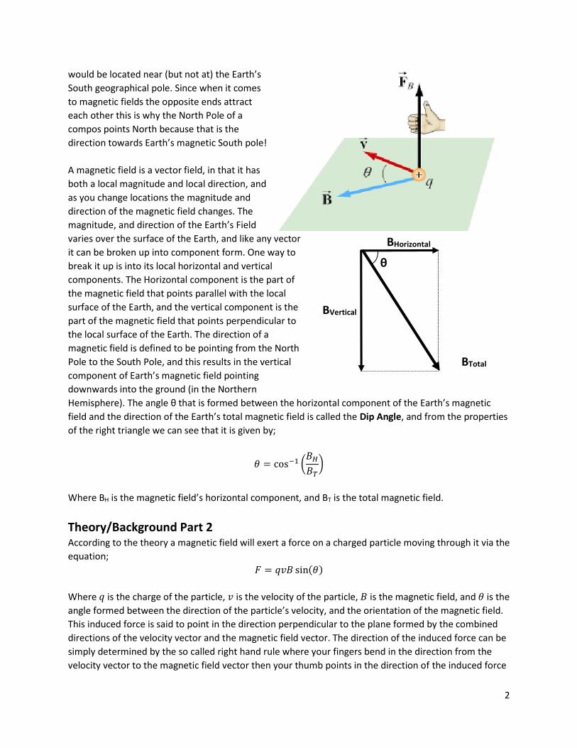
A magnetic field is a vector field, in that it has

both a local magnitude and local direction, and

as you change locations the magnitude and

direction of the magnetic field changes. The

magnitude, and direction of the Earth’s Field

varies over the surface of the Earth, and like any vector

it can be broken up into component form. One way to

break it up is into its local horizontal and vertical

components. The Horizontal component is the part of

the magnetic field that points parallel with the local

surface of the Earth, and the vertical component is the

part of the magnetic field that points perpendicular to

the local surface of the Earth. The direction of a

magnetic field is defined to be pointing from the North

Pole to the South Pole, and this results in the vertical

component of Earth’s magnetic field pointing

downwards into the ground (in the Northern

Hemisphere). The angle θ that is formed between the horizontal component of the Earth’s magnetic

field and the direction of the Earth’s total magnetic field is called the Dip Angle, and from the properties

of the right triangle we can see that it is given by;

𝜃 = cos−1 (𝐵𝐻

𝐵𝑇)

Where BH is the magnetic field’s horizontal component, and BT is the total magnetic field.

Theory/Background Part 2

According to the theory a magnetic field will exert a force on a charged particle moving through it via the

equation;

𝐹 = 𝑞𝑣𝐵 sin(𝜃)

Where 𝑞 is the charge of the particle, 𝑣 is the velocity of the particle, 𝐵 is the magnetic field, and 𝜃 is the

angle formed between the direction of the particle’s velocity, and the orientation of the magnetic field.

This induced force is said to point in the direction perpendicular to the plane formed by the combined

directions of the velocity vector and the magnetic field vector. The direction of the induced force can be

simply determined by the so called right hand rule where your fingers bend in the direction from the

velocity vector to the magnetic field vector then your thumb points in the direction of the induced force

BHorizontal

BVertical

BTotal

θ

3

if the charge is positive, and the force points in the opposite direction of your thumb if the charge is

negative.

If we let a charged particle moving with velocity 𝑣 enter an uniform magnetic field 𝐵 such that the two

vectors are perpendicular to each other, 𝜃 = 900, then the equation reduces too;

𝐹 = 𝑞𝑣𝐵

Once the charged particle enters the magnetic field

the field will exert a force on the particle that is

perpendicular to the directions of both the initial

velocity of the particle and the direction of the field

itself. This results in as the charged particle moves a

little bit into the magnetic field it will begin to turn in

the direction the induced force vector is pointing, but

the particle’s speed does not change. Since the force

vector is pointing in a direction that is perpendicular

to the particle’s initial velocity, and the magnetic field,

the particle’s new velocity after having turned a little

bit will still be perpendicular to the direction of the

magnetic field. Which results in the process repeating,

and then repeating again, and again, and again. The end result being that the particle ends up moving in

a circle of radius 𝑟. The induced magnetic force acts as the centripetal force and any centripetal force

has the form of

𝐹𝑐 = 𝑚𝑣2

𝑟

This allows us to set the two force equations equal to each other.

𝑞𝑣𝐵 = 𝑚𝑣2

𝑟

Helmholz Coils

The apparatus that will be used today employs two Helmholz coils to produce a magnetic field when a

current passes through the wires that make up the coils. This magnetic field will be nearly uniform in the

space between the two coils. This magnetic field is given by

𝐵 = (4

5)

32

∙𝜇0𝑁

𝑅· 𝐼

Where 𝑁 = 130 is the number of loops in each coil, 𝐼 is the current in the coils, 𝑅 = 0.140 𝑚 is the

average radius of the loops in the coils, and the permeability of free space is 𝜇0 = 4 ∙ 𝜋 ∙ 10−7 𝑇∙𝑚

𝐴.

4

A beam of elections will be shot into this magnetic field perpendicular to the field’s orientation. The

electrons are thermally emitted from the heated surface of a cathode and accelerated through a

potential difference ∆𝑉, called the Acceleration Voltage. Assuming the electrons are accelerated from

rest (𝑣𝑖 = 0) then the kinetic energy of the electrons equals the energy they gain as a result of being

accelerated through the potential difference;

1

2𝑚𝑣2 = 𝑒 ∙ ∆𝑉

𝑒 in this equation is the electric charge of the electron, and 𝑚 is the mass of an electron. Solving this

equation for the final speed of the electron we get

𝑣 = √2𝑒 ∙ ∆𝑉

𝑚

Inserting this into our previous equation of the two forces being equal to each other, where 𝑒 = 𝑞, and

solving for 𝑒

𝑚

𝑒𝑣𝐵 = 𝑚𝑣2

𝑟

𝑒𝐵 = 𝑚𝑣

𝑟

𝑒𝐵 = 𝑚√2𝑒 ∙ ∆𝑉

𝑚⁄

𝑟

𝑒2𝐵2 = 𝑚22𝑒 ∙ ∆𝑉

𝑟2 ∙ 𝑚

𝑒

𝑚=

2 ∙ ∆𝑉

(𝐵 ∙ 𝑟)2

5

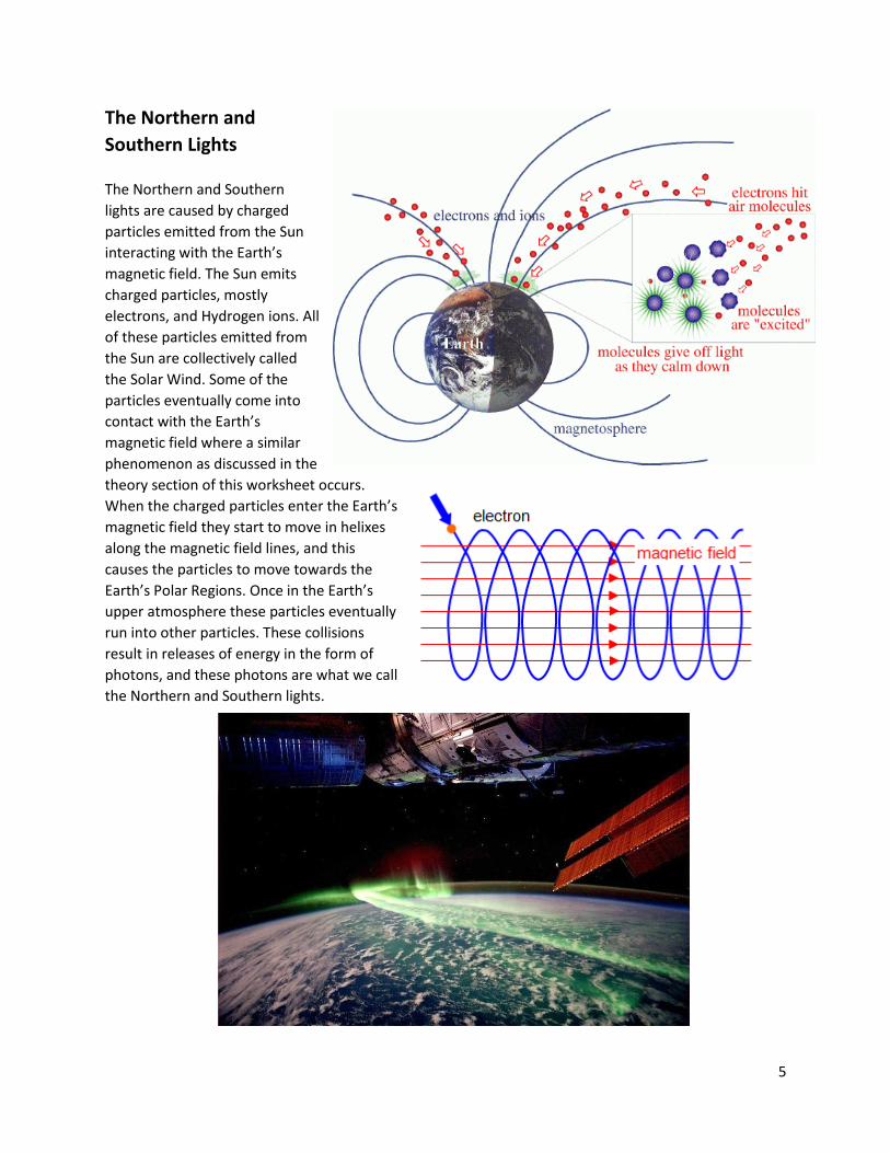
The Northern and

Southern Lights

The Northern and Southern

lights are caused by charged

particles emitted from the Sun

interacting with the Earth’s

magnetic field. The Sun emits

charged particles, mostly

electrons, and Hydrogen ions. All

of these particles emitted from

the Sun are collectively called

the Solar Wind. Some of the

particles eventually come into

contact with the Earth’s

magnetic field where a similar

phenomenon as discussed in the

theory section of this worksheet occurs.

When the charged particles enter the Earth’s

magnetic field they start to move in helixes

along the magnetic field lines, and this

causes the particles to move towards the

Earth’s Polar Regions. Once in the Earth’s

upper atmosphere these particles eventually

run into other particles. These collisions

result in releases of energy in the form of

photons, and these photons are what we call

the Northern and Southern lights.

6

Setup for Part 1

NOTE: During this experiment, keep the apparatus away of all sources of magnetic fields, such as

electronics, computers, bar magnets, and so on. Also keep away from all ferromagnetic materials: iron,

nickel, and cobalt. Best results will be obtained if preformed on a wooden, or hard plastic table.

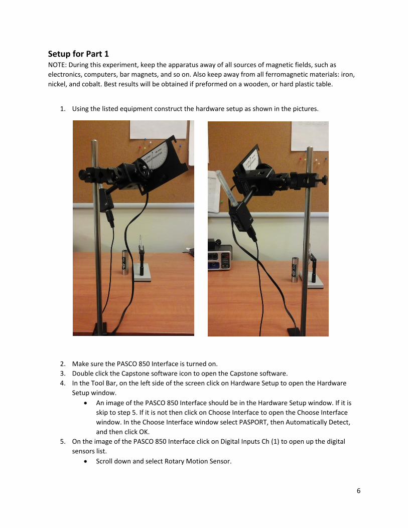
1. Using the listed equipment construct the hardware setup as shown in the pictures.

2. Make sure the PASCO 850 Interface is turned on.

3. Double click the Capstone software icon to open the Capstone software.

4. In the Tool Bar, on the left side of the screen click on Hardware Setup to open the Hardware

Setup window.

An image of the PASCO 850 Interface should be in the Hardware Setup window. If it is

skip to step 5. If it is not then click on Choose Interface to open the Choose Interface

window. In the Choose Interface window select PASPORT, then Automatically Detect,

and then click OK.

5. On the image of the PASCO 850 Interface click on Digital Inputs Ch (1) to open up the digital

sensors list.

Scroll down and select Rotary Motion Sensor.

7

The Rotary Motion Sensor icon should now appear in the Hardware Setup window with

lines indicating that it is selected for Ch (1) and Ch (2)

Plug the Rotary Motion Sensor into the Digital Inputs. Yellow to Ch (1), and black to

Ch(2).

6. On the image of the PASCO 850 interface click on the Analog Inputs Ch (A) to open up the analog

sensors list.

Scroll down and select Magnetic Field Sensor.

The Magnetic Field Sensor icon should now appear in the Hardware Setup window with

a line indicating that is selected for Ch (A).

7. The Gain switch, which is physically on the Magnetic Field Sensor, set it to 100X

8. Make sure orientation switch, which is also physically on the magnetic field Sensor, is set to

Axial.

9. In the Tool Bar click on the Data Summary icon to open the Data Summary window.

In the Data Summary window click on Magnetic Field Strength (100X) (T) to cause a

properties icon to appear to its right.

Click on the properties icon to open the property window.

In the properties window click on Numerical Format.

Set Number of Decimal Places to 3.

Click ok to close the properties window.

10. Close the Tool Bar.

11. Near the bottom center of the screen select Common Rate for the instrument, and then set the

sample rate to 20.0 Hz.

12. In the Display Bar, on the right side of the screen, double click the graph icon to make a graph

appear on Page #1.

Click on Select Measurement for the y-axis, and select Magnetic Field Strength (100X)

(T).

The computer will automatically change the x-axis to time, we need to change the x-axis

to Angle.

Along the x-axis click on Time, then select Angle (rad). Now click on the unts (rad), then

change the units to (o).

8

Procedure for Part 1: Horizontal Component

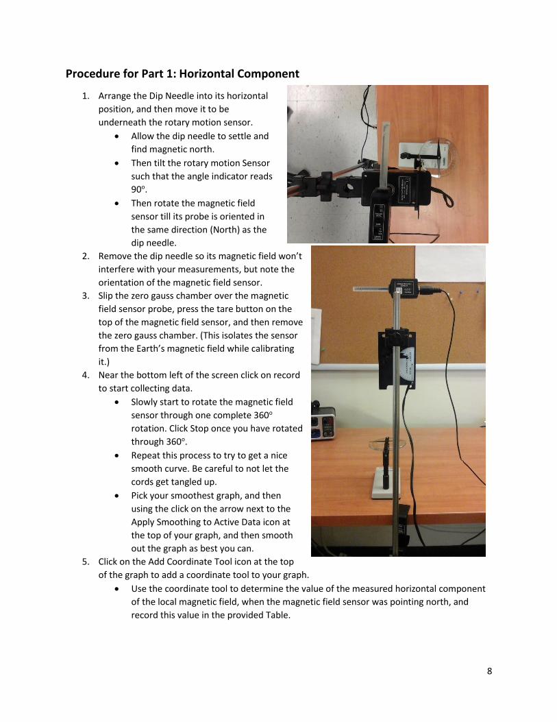
1. Arrange the Dip Needle into its horizontal

position, and then move it to be

underneath the rotary motion sensor.

Allow the dip needle to settle and

find magnetic north.

Then tilt the rotary motion Sensor

such that the angle indicator reads

90o.

Then rotate the magnetic field

sensor till its probe is oriented in

the same direction (North) as the

dip needle.

2. Remove the dip needle so its magnetic field won’t

interfere with your measurements, but note the

orientation of the magnetic field sensor.

3. Slip the zero gauss chamber over the magnetic

field sensor probe, press the tare button on the

top of the magnetic field sensor, and then remove

the zero gauss chamber. (This isolates the sensor

from the Earth’s magnetic field while calibrating

it.)

4. Near the bottom left of the screen click on record

to start collecting data.

Slowly start to rotate the magnetic field

sensor through one complete 360o

rotation. Click Stop once you have rotated

through 360o.

Repeat this process to try to get a nice

smooth curve. Be careful to not let the

cords get tangled up.

Pick your smoothest graph, and then

using the click on the arrow next to the

Apply Smoothing to Active Data icon at

the top of your graph, and then smooth

out the graph as best you can.

5. Click on the Add Coordinate Tool icon at the top

of the graph to add a coordinate tool to your graph.

Use the coordinate tool to determine the value of the measured horizontal component

of the local magnetic field, when the magnetic field sensor was pointing north, and

record this value in the provided Table.

9

Procedure Part 1: Vertical Component

1. Rotate the setup till the

angle indicator reads an

angle of 00.

6. Slip the zero gauss chamber

over the magnetic field

sensor probe, press the tare

button on the top of the

magnetic field sensor, and

then remove the zero gauss

chamber. (This isolates the

sensor from the Earth’s

magnetic field while

calibrating it.)

2. Near the bottom left of the screen click on record to start collecting data.

Slowly start to rotate the magnetic field sensor through one complete 360o rotation.

Click Stop once you have rotated through 360o.

Repeat this process to try to get a nice smooth curve. Be careful to not let the cords get

tangled up.

Pick your smoothest graph, and then using the click on the arrow next to the Apply

Smoothing to Active Data icon at the top of your graph, and then smooth out the graph

as best you can.

3. Click on the Add Coordinate Tool icon at the top of the graph to add a coordinate tool to your

graph.

Use the coordinate tool to determine the value of the measured vertical component of

the local magnetic field, when the magnetic field sensor was pointing downwards, and

record this value in the provided Table.

10

Setup for Part 2

Note: Part 2 will be performed at the lab instructor’s

desk, and under the supervision of the lab instructor.

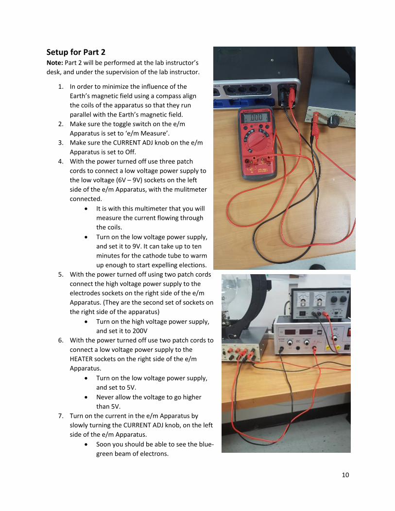
1. In order to minimize the influence of the

Earth’s magnetic field using a compass align

the coils of the apparatus so that they run

parallel with the Earth’s magnetic field.

2. Make sure the toggle switch on the e/m

Apparatus is set to ‘e/m Measure’.

3. Make sure the CURRENT ADJ knob on the e/m

Apparatus is set to Off.

4. With the power turned off use three patch

cords to connect a low voltage power supply to

the low voltage (6V – 9V) sockets on the left

side of the e/m Apparatus, with the mulitmeter

connected.

It is with this multimeter that you will

measure the current flowing through

the coils.

Turn on the low voltage power supply,

and set it to 9V. It can take up to ten

minutes for the cathode tube to warm

up enough to start expelling elections.

5. With the power turned off using two patch cords

connect the high voltage power supply to the

electrodes sockets on the right side of the e/m

Apparatus. (They are the second set of sockets on

the right side of the apparatus)

Turn on the high voltage power supply,

and set it to 200V

6. With the power turned off use two patch cords to

connect a low voltage power supply to the

HEATER sockets on the right side of the e/m

Apparatus.

Turn on the low voltage power supply,

and set to 5V.

Never allow the voltage to go higher

than 5V.

7. Turn on the current in the e/m Apparatus by

slowly turning the CURRENT ADJ knob, on the left

side of the e/m Apparatus.

Soon you should be able to see the blue-

green beam of electrons.

11

Procedure for Part 2

1. Make sure that the high voltage power supply is at 200V. (This is the Acceleration voltage)

2. Using the CURRENT ADJ knob set the current going through the Helmholtz coils till you can see

that the electrons are deflected into a circular path inside the bulb.

Read the current measurement from the multimeter, and record it in the provided

table.

3. Using a measuring ruler measure the radius of the circular beam of electrons, and then record

measurement in the table provided.

Repeat measurements and record in the table provided for four more current settings

each at least 0.10 Amps larger than the previous measurement.

12

Table for Part 1 (20 points)

Horizontal Component of Magnetic Field (T) Vertical Component of Magnetic Field (T)

1. Using your two measured components calculate the magnitude of the local Earth’s magnetic

field. (5 points)

2. The current accepted value of the magnitude of the Earth’s magnetic field in the San Antonio

area is 4.67 ∙ 10−5 𝑇. Calculate the % error between this and your measured value. (5 points)

3. Calculate the Dip Angle of the local Earth’s magnetic field. (5 points)

4. The current accepted value of the Dip Angle of the local Earth’s magnetic field in the San

Antonio area is 58.20 (downwards). Calculate the % error between this and your measured

value. (5 points)

13

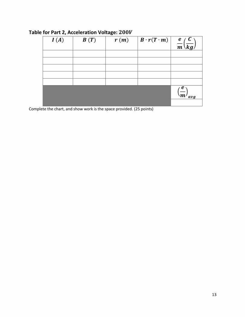
Table for Part 2, Acceleration Voltage: 𝟐𝟎𝟎𝑽

𝑰 (𝑨) 𝑩 (𝑻) 𝒓 (𝒎) 𝑩 ∙ 𝒓(𝑻 ∙ 𝒎) 𝒆

𝒎(

𝑪

𝒌𝒈)

(𝒆

𝒎)

𝒂𝒗𝒈

Complete the chart, and show work is the space provided. (25 points)

14

5. The accepted value of the charge-to-mass ratio of an electron is 𝑒

𝑚= 1.76 ∙ 1011 𝐶

𝑘𝑔

Calculate the % error for your experimental value, and the accepted value. (5 points)

6. Calculate the speed of the elections in our experiment after they have passed through the 200V

acceleration voltage. Now assuming an uniform magnetic field with the magnitude of your

experimental value for Earth’s local magnetic field, what would be the radius of the circular path

that an electron with this speed would make in it? (10 points)