High Reynolds Number Wall Turbulence:Facilities, Measurement Techniques and Challenges

Beverley McKeonGraduate Aeronautical Laboratories

California Institute of Technologyhttp://mckeon.caltech.edu

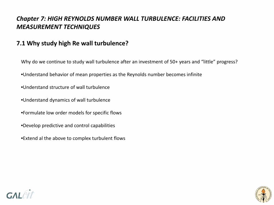
Chapter 7: HIGH REYNOLDS NUMBER WALL TURBULENCE: FACILITIES AND MEASUREMENT TECHNIQUES

7.1 Why study high Re wall turbulence?

Why do we continue to study wall turbulence after an investment of 50+ years and “little” progress?

•Understand behavior of mean properties as the Reynolds number becomes infinite

•Understand structure of wall turbulence

•Understand dynamics of wall turbulence

•Formulate low order models for specific flows

•Develop predictive and control capabilities

•Extend al the above to complex turbulent flows

7.2 Experimental facilitiesComparison of some large‐scale boundary layer wind tunnel facilities

From “The Nordic Wind Tunnel proposal to build a very large turbulence research facility” by W.K. George et al, circa 2001http://www.tfd.chalmers.se/~wkgeorge/TRL/Publications/windtunnel/windtunnels.html

National Diagnostic Facility at IIT Chicago

NASA Ames Full‐Scale Wind Tunnel

(Saddoughi & Veeravalli 1994)

Footprint of large‐scale wind tunnel facilities

Near‐neutral atmospheric surface layer

•Closed loop facility

•Air at pressures up to 200 atmospheres (20 MPa)

•Change in kinematic viscosity, ν, x 160

•Test leg diameter D = 0.12936m

•Development length > 160D

•ReD = 31 x 103 to 35 x 106

•Surface roughness 0.15μm rms

High Reynolds number pipe flow facilities…

Princeton/ONR Superpipe

Comparison of friction factors in Superpipe and Oregon liquid helium facility (mass ratio 25 tonnes/1oz!)

Proposed CICLOPE facility, Bologna, ItalyOsborne Reynolds’ original pipe flow experiment, Manchester, England. ReD~ 3x103

Yamal‐Europe Natural Gas Pipeline

ReD ~ 107

High Reynolds number pipe flow facilities, cont.

•Closed loop facility

•Air at atmospheric pressure

•Test leg diameter D = 0.12936m

•ReD = 31 x 103 to 35 x 106

7.3 Requirements on experimental facilities

•Temperature

•Surface condition

•Flow development (inlet and outlet boundary condition) issues••••

•Pressure gradient

•Freestream turbulence/vibration

•Two‐dimensionality

•Spatial resolution

•Stability (temporal resolution)

7.4 How do we interrogate wall turbulence?

Measurement techniques (not exhaustive)

•Flow visualization

•(Traversing) dynamic pressure profiles

•Hot‐wires

•Sonic anemometry

•Laser Doppler Velocimetry/Anemometry

•Particle Image Velocimetry

•Wall pressure

•Wall shear stress

Visualization:Planar Laser Induced Fluorescence (PLIF) Smoke visualization

Fluorescent dye illuminated using a laser sheet.  Low‐Reynolds number boundary layer, Reθ=725, generated by towing a flat plate in a water tank.  Side and top views. Gad‐el‐Hak (2000)

Smoke illuminated using a laser sheet in the atmospheric surface layer, showing ramp‐like structures.  Comparison with low Reynolds number laboratory boundary layer. Hommema & Adrian (2003)

Measurement of dynamic pressure

])([2)]()([2)( 00 wpypypypyU −≈−=ρρ

Corrections to dynamic pressure measurements: Pitot‐static probes

New displacement correction only

New displacement correction plus wall term

0

5

10

15

20

25

1 10 100 1000 10000

y+

u+

10

15

10 100

y+

U+

What mattered for this study was the slope of the velocity profile (1/κ)

Corrections to stagnation pressure measurements

Pitot pressure• Displacement effect of 

mean shear, O(15%dprobe)

• Turbulence intensity

• Viscous effects

Π=Δpstatic/τw

Corrections to wall static pressure measurementsfinite size of tapping, ΔU = O(1%U)

Effect of McKeon & Smits static pressure correction

22

24

26

28

30

32

34

36

1000 10000 100000 1000000y+

u+

Re = 3M

Re = 13M

k=0.421,B=5.60

McKeon & Smits, Meas. Sci. Tech., 13, 2002

Effect of McKeon & Smits static pressure correction

22

24

26

28

30

32

34

36

1000 10000 100000 1000000y+

u+

Re = 3M

Re = 13M

k=0.421,B=5.60

McKeon & Smits, Meas. Sci. Tech., 13, 2002

If you only have low Reynolds number data then appropriate Pitot probe corrections are crucial.

With high Reynolds number data the corrections become small

With wall term

Old static pressure correction and new displacement correction

New static pressure correction and new displacement correction

Effect of corrections on overlap region scaling

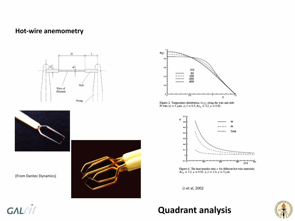
Quadrant analysis

Hot‐wire anemometry

(From Dantec Dynamics)

Li et al, 2002

Issues associated with 

• calibration

• frequency response of combined wire/circuit system

• noise floor

• temperature drift

• spatial resolution

(From Dantec Dynamics)

(From Bruun 1995)

h 0.97 h

0.15 ht

fc

=1.3 τ

w

τw

1

Hot‐wire anemometry, cont.

NSTAP – Kunkel, Arnold & Smits 2006

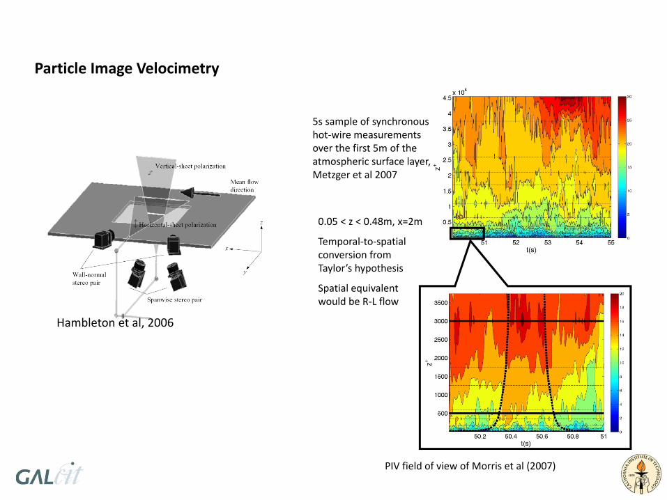
Particle Image Velocimetry

Hambleton et al, 2006

PIV field of view of Morris et al (2007)

0.05 < z < 0.48m, x=2m

Temporal‐to‐spatial conversion from Taylor’s hypothesis

Spatial equivalent would be R‐L flow

5s sample of synchronous hot‐wire measurements over the first 5m of the atmospheric surface layer, Metzger et al 2007

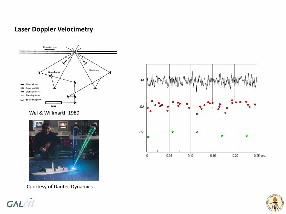
Wei & Willmarth 1989

Courtesy of Dantec Dynamics

Laser Doppler Velocimetry

Kalvesten thesis, 1996

Klewicki et al, 2008

Wall pressure Wall shear stress

ѵ – kinematic viscosity of oil at 22.5˚C [72.5 ˚F] =55E‐6 m^2/s λ – wavelength of sodium light source =  589 nmn – index of refraction for oil = 1.402ρ – density of oil = 0.963 kg/Lds/dt – rate of change of fringe width

Chandrasekan et al, 2005

Jacobi et al, 2009!