HIGH REYNOLDS NUMBER ANALYSIS OF FLAT …mln/ltrs-pdfs/NASA-aiaa-96-2544.pdfhigh reynolds number analysis of flat plate and separated afterbody flow using non-linear turbulence models

HIGH REYNOLDS NUMBER ANALYSIS OF FLAT PLATE ANDSEPARATED AFTERBODY FLOW USING NON-LINEAR TURBULENCE MODELS

John R. Carlson�

NASA Langley Research CenterHampton, VA

Abstract

The ability of the three-dimensional Navier-Stokesmethod, PAB3D, to simulate the e�ect of Reynolds num-ber variation using non-linear explicit algebraic Reynoldsstress turbulence modeling was assessed. Subsonic at plateboundary-layer ow parameters such as normalized veloc-ity distributions, local and average skin friction, and shapefactor were compared with DNS calculations and classicaltheory at various local Reynolds numbers up to 180 million.Additionally, surface pressure coe�cient distributions andintegrated drag predictions on an axisymmetric nozzle af-terbody were compared with experimental data from 10 to130 million Reynolds number. The high Reynolds data wasobtained from the NASA Langley 0.3m Transonic CryogenicTunnel. There was generally good agreement of surfacestatic pressure coe�cients between the CFD and measure-ment. The change in pressure coe�cient distributions withvarying Reynolds number was similar to the experimentaldata trends, though slightly over-predicting the e�ect. Thecomputational sensitivity of viscous modeling and turbu-lence modeling are shown. Integrated afterbody pressuredrag was typically slightly lower than the experimental data.The change in afterbody pressure drag with Reynolds num-ber was small both experimentally and computationally,even though the shape of the distribution was somewhatmodi�ed with Reynolds number.

Introduction

Current focused program e�orts are considering Reynoldsnumber scaling a signi�cant aspect of aircraft testing anddevelopment. Wing aerodynamics and ow about propul-sion systems can have considerable sensitivity to varyingReynolds number. Most of the sub-scale wind tunnel testingoccurs at Reynolds numbers below that of ight conditions;therefore, the ability of computational uid dynamics (CFD)to simulate higher Reynolds number ow is of importance.

Previous to the development of cryogenic test techniquesfor achieving high Reynolds numbers in wind tunnel facili-ties, little fundamental research data had been available forthe evaluation of any theoretical methods to predict thesee�ects. Several years ago, during the development phase ofcryogenic testing techniques at the NASA Langley ResearchCenter; two sets of simple axisymmetric nacelle models werebuilt and tested in what was then known as the 1/3m PilotTransonic Cryogenic Tunnel (now the 0.3m Transonic Cryo-genic Tunnel). This was some of the �rst set of test data

�Senior Scientist, Component Integration Branch, Aerodynamics Division. Senior

Member AIAA.

Copyright c 1996 by the American Institute of Aeronautics and Astronautics, Inc.

No copyright is asserted in the United States under Title 17, U.S. Code. The U.S.

Government has royalty-free license to exercise all rights under the copyright claimed

herein for Governmental purposes. All other rights are reserved by the copyright owner.

for nozzle-boattail geometries taken over a large range ofReynolds numbers, refs. 1{4.

The current investigation assesses the capability of theNavier-Stokes method PAB3D, version 13S, (refs. 5{8) usingnon-linear algebraic Reynolds stress turbulence models topredict the Reynolds number e�ects on the ow about anozzle boattail. and simulate a 5 meter at plate at veryhigh Reynolds numbers. Comparisons were made with windtunnel data for the boattail geometry and boundary layerpro�les, shape factor, and skin friction with DNS data andtextbook equations for incompressible at plate ow.

Nomenclature

Amax maximum body cross-sectional area,

0.78539 in2

CD pressure drag coe�cient, Fq1Amax

CF average skin friction coe�cient,1lq1

P�w�l

Cf local skin friction coe�cient, �w=q1

Cp pressure coe�cient, p�p1q1

dm body maximum diameter, 1.0 in.

F axial force along body axis

f� near-wall damping function for linearK � "

GS Gatski-Speziale

H12 boundary layer shape factor, �1=�2

H32 boundary layer shape factor, �3=�2

h1 physical height of �rst computationalgrid from a wall

K turbulent kinetic energy

l integration length of at plate

L model reference length

M Mach number

NRe Reynolds number based on model refer-ence length

n direction normal to wall

P production term for turbulent kineticenergy

p static pressure, Pa

q dynamic pressure, Pa

RL Reynolds number based on at plateintegration length

RT cell turbulent Reynolds number, K2=��

Rx Reynolds number based on distance x,u1x=�

1

Americal Institute of Aeronautics and Astronautics

R�1displacement thickness Reynolds number,u1�1=�

R� momentum thickness Reynolds number,u1�2=�

t time

S strain tensor

SZL Shih, Zhu & Lumley

U magnitude of local velocity,pP

uk2

u stream-wise velocity

uk cartesian velocity components

u+ law-of-the-wall coordinate, u=u�

u� friction velocity,p(�w=�)

u0v0+ nondimensional shear stress, u0v0=u�2

W vorticity tensor

x stream-wise distance

y+ law-of-the-wall coordinate, nu�=�

z vertical distance

�l incremental distance on at plate

�1 boundary layer displacement thickness

�2 boundary layer momentum thickness

�3 boundary layer energy thickness

� turbulent dissipation

� laminar viscosity

�t turbulent viscosity

�w local laminar viscosity at the wall

� kinematic viscosity, �=�

� density

� shear stress

� angular location of pressure ori�ces, deg

Superscripts

L laminar

T turbulent

Subcripts

� nozzle boattail component contribu-tion

CL centerline

fp at plate

l laminar

n non-linear component

t turbulent

t0 free stream total condition

sf skin friction contribution

w;wall condition at the wall surface

1 free stream condition

Computational Procedure

Governing Equations

The code used was the general three dimensional (3-D)Navier-Stokes method PAB3D, version 13S. This code hasseveral computational schemes, di�erent turbulence models,and viscous stress models that can be utilized, as describedin more detail in refs. 5 through 8. The governing equationsare the Reynolds-averaged simpli�ed Navier-Stokes equa-tions (RANS) obtained by neglecting all stream-wise deriva-tives of the viscous terms. The resulting equations arewritten in generalized coordinates and conservative form.Viscous model options include k-thin layer, j-thin layer,jk-uncoupled and jk-coupled simulations. Typically the thin-layer viscous assumption of the full 3-D viscous stresses isutilized. Experiments such as the investigation of super-sonic ow in a square duct was found to require fully cou-pled 2 directional viscosity to properly resolve the physicsof the secondary cross- ow. The Roe upwind scheme with�rst, second, or third order accuracy can be used in evalu-ating the explicit part of the governing equations and thevan Leer scheme is used to construct the implicit operator.The di�usion terms are centrally di�erenced and the inviscid ux terms are upwind di�erenced. Two �nite volume ux-splitting schemes are used to construct the convective uxterms.

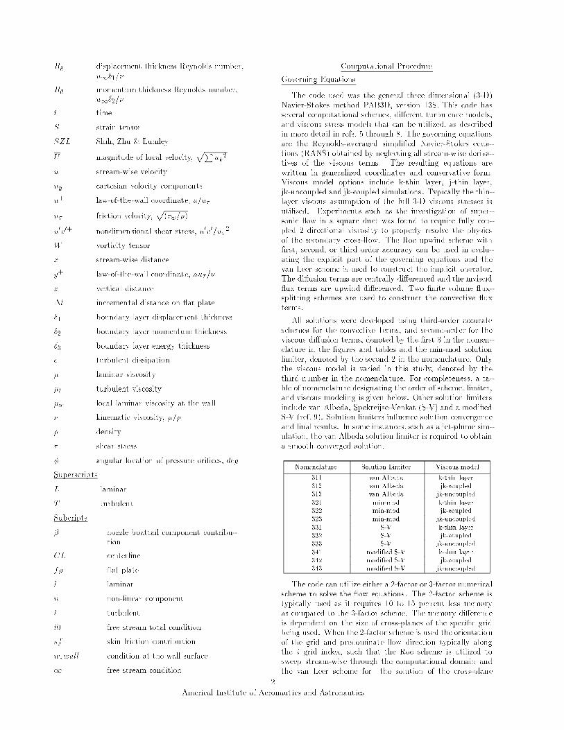
All solutions were developed using third-order accurateschemes for the convective terms, and second-order for theviscous di�usion terms, denoted by the �rst 3 in the nomen-clature in the �gures and tables and the min-mod solutionlimiter, denoted by the second 2 in the nomenclature. Onlythe viscous model is varied in this study, denoted by thethird number in the nomenclature. For completeness, a ta-ble of nomenclature designating the order of scheme, limiter,and viscous modeling is given below. Other solution limitersinclude van Albeda, Spekreijse-Venkat (S-V) and a modi�edS-V (ref. 9). Solution limiters in uence solution convergenceand �nal results. In some instances, such as a jet-plume sim-ulation, the van Albeda solution limiter is required to obtaina smooth converged solution.

Nomenclature Solution Limiter Viscous model

311 van Albeda k-thin layer

312 van Albeda jk-coupled

313 van Albeda jk-uncoupled

321 min-mod k-thin layer

322 min-mod jk-coupled

323 min-mod jk-uncoupled

331 S-V k-thin layer

332 S-V jk-coupled

333 S-V jk-uncoupled

341 modi�ed S-V k-thin layer

342 modi�ed S-V jk-coupled

343 modi�ed S-V jk-uncoupled

The code can utilize either a 2-factor or 3-factor numericalscheme to solve the ow equations. The 2-factor scheme istypically used as it requires 10 to 15 percent less memoryas compared to the 3-factor scheme. The memory di�erenceis dependent on the size of cross-planes of the speci�c gridbeing used. When the 2-factor scheme is used the orientationof the grid and predominate ow direction typically alongthe i grid index, such that the Roe scheme is utilized tosweep stream-wise through the computational domain andthe van Leer scheme for the solution of the cross-plane

2


(i.e., i = constant) of a 3-D problem. However solving asingle-cell wide two-dimensional (2-D) mesh de�ned withthe i direction of the grid oriented in the conventionalstream-wise direction will typically converge slower usingthe Roe relaxation solution scheme compared to solving theequivalent problem with the van Leer scheme. Therefore thei and j directions of a 2-D mesh are swapped allowing theentire ow-�eld to be solved implicitly with each iteration.The explicit sweep is not used since only one cell exists in thei direction. The implicit scheme usually has a much higherrate of convergence and typically provides a solution usingless computational time.

Turbulence Simulation

The turbulence model equations are uncoupled from theRANS equations and are solved with a di�erent time step,typically 1/2, than that of the principle ow solution. Aconsiderably lower principle Courant-Friedrichs-Levy (CFL)number is typically required to solve problems if both themain ow equations and turbulence equations are solved it-eratively using identical time rates. Larger time step di�er-ences, e.g., 1/4 to 1/8, slow solution convergence further butresult in identical �nal solutions. Flow solution transients attimes require the turbulence equations time step to be re-ducted temporarily. Turbulence simulations are resolved atall grid levels, not just at the �nest grid level.

Version 13S of the PAB3D code used in this study hasoptions for several algebraic Reynolds stress (ASM) turbu-lence simulations. The Standard model coe�cients of theK � " equations were used as the basis for all the linear andnon-linear turbulent simulations, ref. 10. Additionally, it isknown that the eddy viscosity models produce inaccuratenormal Reynolds stresses. Flat plate ow, as well as othermore complex aerodynamic ows, are anisotropic.

Successful implementation of the algebraic Reynoldsstress models required the solution methodology for turbu-lent production term P of the underlying linear turbulencecalculations to be modi�ed. P depends on high order deriva-tives of the turbulent Reynolds stresses. Proper represen-tation of the stresses should be provided by face centeredvalues, rather than the cell centered values. Previous at-tempts to implement non-linear turbulence models in thecontext of a cell centered eddy viscosity model worked onlyfor 2-D problems and was unable to resolve 3-D ows.

Linear K � " equations|The transport equation for theturbulent kinetic-energy, K, and the dissipation rate arewritten as:

@"

@t+ uk

@"

@xk=

@

@xk

�(�L + C�

K2

")@"

@xk

�

+ C"1"P

K� C"2

"

K

24"� 2�

@pK

@n

!235(1)

The convective terms are solved using third-order di�er-encing. The di�usion terms are solved using second-ordercentral di�erencing.

@K

@t+ uk

@K

@xk= P � " +

@

@xk

�(�L + C�

K2

")@K

@xk

�(2)

where P = �Tik

@ui

@xkand (C"1=1:44; C"2=1:92; C�=0:090):

The damping function of Launder & Sharma, ref. 11,

f� = exp��3:41=(1 + RT=50:)

2�, determined the behavior

of " near the wall as a function of turbulent Reynolds numberRT = K2=�". The boundary conditions for " and K at

the wall are "wall = 2��

@

@n

pK�2

and Kwall = 0. The

stress components in linear turbulence models are developedwith laminar and turbulent components, �ij = �L

ij+ �T

ij. A

generalization of Boussinesq's hypothesis rede�nes laminarand turbulent components are as follows:

�Lij= AL�ij � 2�LSij (3)

where

AL =2

3�LSkk and Sij =

1

2

�@ui@xj

+@uj

@xi

�(4)

The turbulent component of the stresses �Tij

is repre-

sented by the sum of linear (Tl) and non-linear (Tn) compo-

nents. The linear stress is �Tl

ij= AT �ij � 2�TSij where

AT = 2

3(�K + �TSkk). The non-linear component of the

turbulent stresses are addressed in the following section.

Non-Linear Turbulent Stress Equations|Three theoriesof explicit algebraic Reynolds stress models were imple-

mented. The Reynold's stress contribution �Tn

ijused by

Shih, Zhu, & Lumley (SZL), (ref. 12) is;

�Tnij

= 2�K3

�2

�WikSkj � SikWkj

�(5)

Gatski & Speziale (GS), (ref. 13);

�Tnij

= C��K3

"2

��1(WikSkj � SikWkj) + �2(SikSkj

�1

3SmnSmn�ij)

�(6)

and Girimaji (G), (ref. 14);

�Tnij

= 2C��K3

"2

��G2

�WikSkj � SikWkj

�+ G3(SikSkj

�1

3SmnSmn�ij)

�(7)

where

Wij =1

2

�@ui@xj

�@uj

@xi

�

Sij = Sij �1

3Skk�ij

The turbulent viscosity, �T , is de�ned as

�T = C��

��K2

�

�(8)

3


where C�� = f�C� for solutions solving linear turbulence sim-ulations and equal to the variable function C�

� = f(S;W;K; ")for solutions involving algebraic Reynolds stress simulations.Functions for C�

� take the following forms for each of theASM.

Shih, Zhu & Lumley, (ref. 12):

C�� = 1=

�6:5 + A�s

U�K�

�(9)

Gatski-Speziale, (ref. 13):

C�� = const: � (1 + �2)=(3 + �2 + 6�2 2 + 6 2) (10)

A�s , U� , �, and are all di�erent functions of the strainand vorticity tensors and are detailed in the references.

Girimaji, (ref. 14):

G1 =

8>>>>>>>>>>>><>>>>>>>>>>>>:

L10L2=

�(L0

1)2 + 2�2(L4)

2�

for �1 = 0;

L10L2=

�(L0

1)2 + 2

3�1(L3)2 + 2�2(L4)

2�

for L11 = 0;

� p3 +

�� b

2 +pD� 1

3+�� b

2 �pD� 1

3for D > 0;

� p3 + 2

q�a3 cos( �3 ) for D < 0 and b < 0;

� p3 + 2

q�a3 cos( �3 +

2�3 ) for D < 0 and b > 0.

(11)

The variable G1 utilized by Girimaji is equal to �C��.

A compilation of the parameters used in Girimaji's modelcan be found in the Appendix. Additional information is inreference 14.

The solution processes for wall-bounded ows wereequally robust for each of the models. Previous results, notpublished here, show Gatski-Speziale requiring lower CFLnumbers for the solution of free-shear ows. Obtaining con-verged solutions using Gatski's C�

� were found to be problemdependent. Girimaji's G1 function appears to be extremelywell behaved permitting for fairly high CFL numbers toused.

Turbulent Trip Equations|The technique used for initial-izing the viscous ow transition from laminar to turbulent isplacing K and " pro�les at user-speci�ed lines or planes in the ow�eld. The line or plane of the speci�ed trip area is sur-veyed for the maximum and minimum velocity and vorticityalong that line and a shape function from 0 to 1 is created ofthe form F = (f � fmin)=(fmax � fmin) where f is a prod-

uct of the velocity and vorticity f = ujW j; jW j = 2qP

W2ij .

The turbulent kinetic energy pro�le is then K = � U F ,where � is a free parameter determining the magnitude ofthe impulse as a percent of local total velocity, U . The typi-cal value speci�ed by the user, and used for this paper, is 2%(or � = 0:02). The " pro�le is developed from the assump-tion that production P is equal to the dissipation " equaling

C�K2

" 2�Sij@ui@xj

. The result of the initialization is seen as a

spike in the K �eld of the solution. This initial turbulentpro�le develops as permitted by the local ow conditions.

Solution Process

Turbulent ow solutions using ASM and two-equationlinear K � � model requires 23 words per grid point. Thecode speed is dependent on the turbulence model, thin-layerassumptions and numerical schemes. The following tableare some options available in the code with C-90 timing in�seconds/iteration/grid point.

Turbulence

Solver Scheme Viscous Modeling Stress Timing C-90

Modeling (3rd-order) Center �s/iter/grid

2-factor j-k uncoupled Girimaji ASM Face 23

2-factor k thin-layer Girimaji ASM Face 20

Diagonalization j-k uncoupled Girimaji ASM Face 16

Diagonalization k thin-layer Girimaji ASM Face 14

2-factor k thin-layer Gatski & Face 19

Speziale ASM

2-factor k thin-layer SZL ASM Face 20

2-factor k thin-layer Linear-Isotropic Face 18

2-factor k thin-layer Linear-Isotropic Cell 17

Diagonalization k thin-layer Linear-Isotropic Face 12

Several parameters were used to gauge solution conver-gence. Local skin friction, shape factor and solution residualwere monitored for convergence of the at plate solutions.Total afterbody drag, nozzle pressure drag, and solutionresidual were used to determine the solution status at thecoarse (144), medium (122), and �ne (111) grid levels of theaxisymmetric afterbody. The 144 abbreviation means dividenumber of i-cells by 1, number of j-cells by 4 and the numberof k-cells by 4. Afterbody drag variance of less than 0.50 per-cent for several hundred iterations was achieved for all testcases.

The conservative patch interface package of Pao andAbdol-Hamid (ref. 7) enables the code to properly transmitinformation between mis-matched block interfaces. Integer-to-one interfaces are considered a subset of the arbitraryblock interface and do not need to be speci�ed as such tothe patching code. The patching program is a preprocessorthat writes a connectivity data base prior to the start of the�rst solution. Each entry to the patch data base containscell face areas and indices relating that cell with all othercells that will share momentum ux information. The database information is automatically re-allocated internal to thecode during mesh sequencing. As a result, each block canbe sequenced at di�erent levels and the correct interfaceinformation is maintained at the cell level. However, it isimportant to note that features in the ow developed on oneside of an interface should not be obliterated on the otherside due to an excessive grid density mis-match.

Third-order continuity in transmitting the uxes acrossblock boundaries is maintained by the code; lower ordercontinuity may be speci�ed by the user if required. Aswith most Navier-Stokes methods of the type, equal cell sizespacing on either side of an interface in directions normalto the interface should be maintained regardless of the meshsequencing level of the block.

Boundary Conditions

For this study, solid walls were treated as no-slip adiabaticsurfaces. The solid wall boundary condition was satis�edby setting the momentum ux of the solid wall cell face

4


to zero. A boundary condition for the Riemann invariantsalong the characteristics was speci�ed for the free-streamin ow face and the lateral free-stream outer boundary ofthe ow domain. An extrapolation boundary condition wasapplied on the downstream out ow face. The axisymmetric ow assumption for the single-cell grids was implementedby placing ow symmetry conditions to the lateral sideboundaries of the computational domain.

Results and Discussion

Subsonic Flat Plate

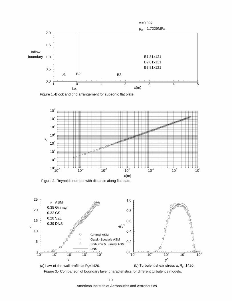
Flat Plate Grid|The 5 m at plate multiblock grid hadan H-type mesh topology, with the blocking sketched in�gure 1. The computational domain included in ow blockextending 1 meter upstream from the leading edge of the 5m at plate. The initial stream-wise grid spacing at theleading edge of the plate was 1:�104m and was exponentiallystretched from the leading edge to the trailing edge at arate of 5% with a total of 161 grid points. The �rst cellheight was 1:0 � 106 m �xed at both ends of the plateand exponentially stretched from the surface to the outerboundary at a rate of 11% with a total of 121 grid points.The upper boundary was 2 m away and the lateral widthof the grid of 0.01 m. All three blocks had dimensionsof 81 � 121. Tripping to turbulent ow simulation occurredaround Rx = :3 million or R�1 = 900, corresponding to aphysical distance of approximately 9 mm downstream ofthe plate leading edge. This allowed for laminar ow tooccur over roughly 32 computational cells before tripping toturbulent ow. Grid cell counts were divisible by four toallow a minimum of 2 levels of grid sequencing.

Boundary Layer Characteristics|Figure 2 shows theReynolds number based on length variation with distancefrom the leading edge. The Reynolds number at the platetrailing edge was approximately 180 million. Note that theplot is a log-log type with the symbols indicating the stream-wise distribution of the grid points. The high Reynoldsnumber was obtained through increasing the free-streamtotal pressure, rather than physically lengthening the atplate geometry. The normalized velocity and shear stressdistributions at R� = 1420 and 100,000 are shown in �g-ures 3 and 4. The comparisons at R� = 1420 are com-pared with the DNS calculations of Spalart, ref. 15, andat R� = 100; 000 are compared with the classical at plateequations. All three ASM match fairly closely the DNScalculation shown in �gure 3, with the Girimaji model fol-lowing the closest in the bu�er region. All three modelswere slightly above the DNS at the edge of the bound-ary layer. Similarly, Girimaji best �t the DNS stress pro-

�le, u0v0+ = (@u=@z)C�f�K2="=u� , though all three ASM

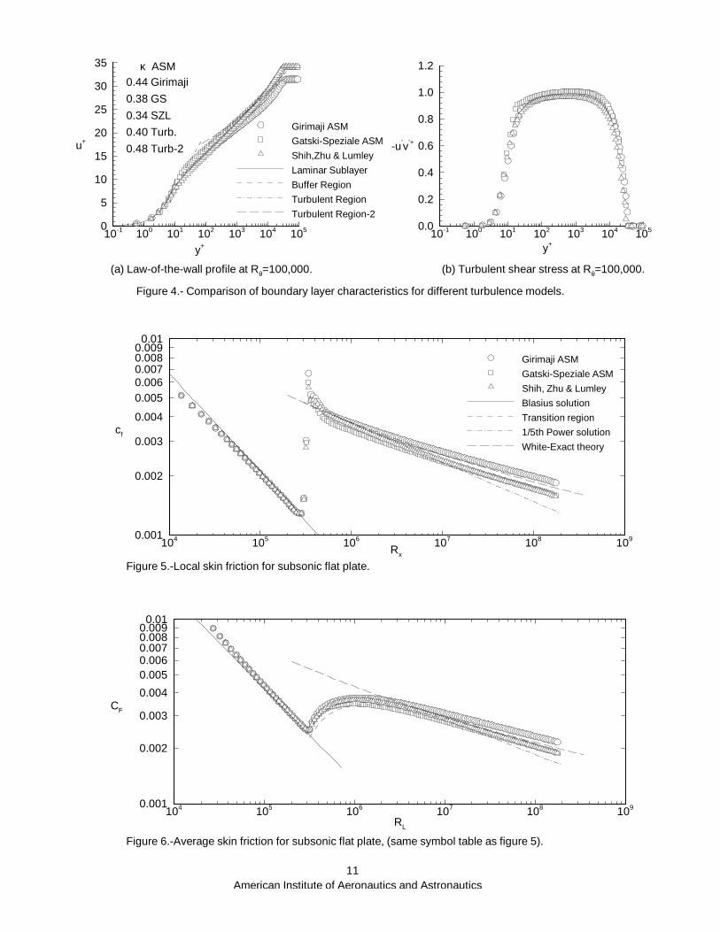
were generally a good match. The high Reynolds num-ber comparisons, �gure 4, at R� = 100; 000, approximatelyNRe = 90 million, have trends fairly consistent with the clas-sical at plate boundary layer ow equations. The stresspro�les, �gure 4(b), have similar lower level behavior (be-low y+ = 50) as the lower Reynolds number pro�les and agreatly attened region of constant stress below the bound-ary layer edge around y+ = 30; 000. The grid had typically 2cells less than y+ = 2:5 and about 36 cells in the boundarylayer at R� = 1420.

Flat Plate Skin Friction|Figures 5 and 6 are a compari-son of classical at plate theories for local and average skin

friction with the three ASM solutions. The equations for thelocal skin friction comparisons were:

cf =

8>><>>:

0:664=pRx; Blasius ;

0:0590Rx�15 ; 1

5th power law;

0:455=ln2(0:06Rx); White-\Exact" theory.

(12)

The equations for the average skin friction were:

CF =

8>>>>><>>>>>:

1:328=pRL; Blasius;

0:455=(log2:5810 (RL)�A=RL); Transition;

0:074RL� 15 �A=RL;

15th power law;

0:523=ln2(0:06RL); White-\Exact" theory.(13)

where A = Rcrit(CFt�CFl

), CFl= 1:328=

pRcrit, CFt

=

0:074(Rcrit)�15 .

Rcrit is the local Reynolds number at the point of transi-tion from laminar to turbulent ow. Transition was de�nedas the point at which the shape factor H12 �rst fell below2.3. Local skin friction and average skin friction coe�cientsand normalized turbulent viscosity are plotted in �gures 7, 8and 9, respectively for all three of the algebraic Reynoldsstress models. Girimaji, SZL and GS ASMs predict sim-ilar and consistent skin friction characteristics throughoutthe Reynolds number range. All three models were virtuallyidentical in local and average skin friction for the laminar ow that developed upstream of the transition trip point atRx = 300; 000. Downstream of the trip, the Girimaji modeldeveloped slight higher local skin friction that the other twoASM, with subsequently higher average skin friction. Allthree models departed from the 1/5th power theory for localskin friction at Reynolds numbers above 20 million. The skinfriction predicted by Girimaji's model was slightly above thehigher Reynolds number theory of White, while the othertwo tracked slightly low.

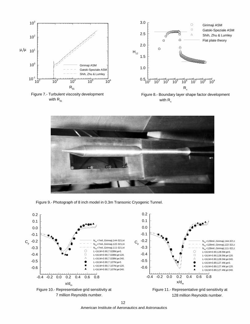
The trend of average skin friction through transitionto turbulent ow was similar between the three modelsand followed the 1/5th power theory very closely until,again departing around 20 to 30 million Reynolds number,�gure 6. Figure 7 is a plot of the growth of turbulentviscosity normalized by the local laminar viscosity with R�1 .Girimaji's model predicts the highest level of normalizedturbulent viscosity, though all three models are very similarin level and rate of growth.

Boundary Layer Shape Factors|All three ASM have verysimilar shape factor H12 trends as shown in �gure 8. The�rst 8 or so computational cells were neither laminar norturbulent as the solution developed. The subsequent 28cells matched the theoretical laminar characteristics veryclosely. The theoretical turbulent shape factor was notclosely achieved until around Rx = 20 million. Even thoughtransition from laminar ow occured relatively quickly, for-mation of a turbulent shape factor close to the theoreticalshape required some distance to achieve. All three modelsvery closely match the turbulent shape factor of H12 = 1:27at very high Reynolds numbers.

Overall, all three non-linear turbulence models appear tobe consistent and well behaved turbulent at plate proper-ties up to Reynolds numbers of 180 million.

5


Axisymmetric Afterbody

Test Facility|The second test case was an axisymmet-ric geometry that was part of a series of models testedin both the Langley 1/3m Pilot Transonic Cryogenic Tun-nel and the 16-Foot Transonic Tunnel. The Pilot Tunnelhad an octagonal test section with slots at the corners ofthe octagon and is essentially a scale model of the Lang-ley 16-Foot Transonic Tunnel test section, ref. 16. The testmedium for the cryogenic tunnel was nitrogen cooled by liq-uid nitrogen. High Reynolds number data were obtained inthe 0.3m tunnel through a combination of cryogenic free-stream temperatures and free-stream total pressure that areindependently controllable. Approximately 5 atm. of pres-sure and 100K total temperature produced a unit Reynoldsnumber of 260 million/meter.

The experiment was conducted over a range of tempera-tures from approximately 100K to 300K and pressures from 1to 5 times the standard atmospheric level. Several settingsof free-stream total temperatures or pressures can result inidentical settings of Reynolds number. Surface pressure co-e�cients and nozzle boattail drag were shown to be simi-lar regardless of the temperature/pressure combinations thatcreated equivalent Reynolds numbers, ref. 2. High Reynoldsnumber simulations with the CFD method were obtainedthrough increased total pressure rather than through a com-bination of free-stream total pressure and cryogenic tem-peratures. Though data were obtained over range of Machnumber from 0.6 to 0.9, only the M = 0:9 data is comparedwith the CFD in this paper. The following is a table ofconditions for experimental data obtained at M = 0:9 forthe L=dm = 16:0 model. One atmosphere is de�ned at0.101325 MPa (14.703 psi).

M1

Tt0 ,K(R) pt0 ,atm NRe � 106

.903 106 (191) 4.98 128

.908 118 (212) 3.98 87

.901 119 (214) 2.98 64

.911 118 (212) 2.47 55

.910 118 (212) 1.97 43

.904 119 (214) 1.49 32

.903 118 (212) 1.24 27

.899 312 (562) 4.97 28

.899 308 (554) 3.79 22

.902 308 (554) 2.48 14

.901 307 (553) 1.23 7

Geometry|The con�guration used for this study wasone of six models that were built for the original Reynoldsnumber study, ref. 1. Four models with di�ering boattailgeometry were associated with a body length of 8 inchesfrom the nose to the start of the boattail (characteristiclength) and two models with a characteristic length of 16inches. The boattail geometries had circular arc, circulararc-conic, or contoured pro�les. This investigation utilizedthe circular arc with a length-to-maximum-diameter ratio(�neness ratio) of 0.8 boattail. Figure 9 is a photographof the model mounted in the pilot tunnel. The nose ofthe model was a 28� cone 1.7956 inches long fairing to thecylindrical body via a 1.3615 inch radius circular arc whosecenter is 2.125 downstream of the model nose and 0.8615inches below the model centerline. The circular arc fairingis tangent at its endpoints to the conical nose (1.7956 inchesfrom the nose) and cylindrical body (2.125 inches from the

nose). The model was sting mounted with the diameterof the sting being equal to the model base diameter. Thelength of the constant diameter portion of the sting (6.70inches measured from the nozzle connect station) was suchthat, based on the work of Cahn, ref. 17, there should beno e�ect of the sting are downstream of the nozzle trailingedge on the boattail pressure distributions.

The axisymmetric afterbody grid utilized H-O type meshtopology with all block dimensions that were divisible by 4.The mesh was gridded with a single cell 5 degree wide wedgegrid with the stream-wise ow direction oriented along the jindex to utilize the implicit ow solver in the code for fastersolution convergence. The body was described using 100cells extending from the leading edge of the nose to the nozzleconnect station. There were 80 cells extending from thenozzle connect station to the nozzle boattail trailing edge.

The free-stream conditions for axisymmetric CFD caseswere M = 0:9, Tt0 = 540R using air at = 1:4: The �rstcell height of each con�guration's grid was di�erent foreach free-stream Reynolds number according to the followingschedule.

Reynolds number pt0,atm. (psi.) h1 (inches)

7 . . . . . . 1.2 (17.8) 6�10�5

55.2 . . . . 9.52 (140.) 8�10�6

128.3 . . . . 22.1 (325.) 2�10�6

The wind tunnel models were constructed of cast alu-minum with stainless-steel pressure tubes cast as an integralpart of the model. The model was instrumented with 30pressure ori�ces in three rows of 10 ori�ces each. The 1 inchdiameter of the model physically precluded the placementof all 30 ori�ces along the same row. The following is atabulation of the non-dimensional ori�ce locations.

x/dm for L/dm = 16 at

� = 0� � = 120

� � = 240�

-0.4491 -0.4660 -0.4561

-.1637 -.2201 -.1552

-.0600 -.1281 -.0590

.0337 -.0260 .0390

.1268 .0744 .1342

.2279 .1729 .2713

.3210 .2696 .3718

.4199 .3679 .4680

.5231 .4640 .5749

.6279 .6758 .7304

Grid convergence|Figures 10 and 11 show grid sensitiv-ity of the Girimaji ASM at M = 0:9 at the lowest and highestReynolds number for this test case, NRe = 7 and 128 million,respectively. These sensitivities were relatively consistent forthe other turbulence models and other viscous models inves-tigated. A few exceptions occurred where the coarse gridsolution did not converge, but the following medium and�ne grid solutions converged and the results were similar innature as those shown in �gures 10 and 11. All solutionswere fairly well grid converged and solution converged. Ini-tial inspection of �gure 11, the coarse grid solution has theclosest match with the data. Further re�nement of the gridrevealed this solution to not be grid converged. Convergedsolutions for this geometry appear to require between 40

6


to 80 cells along the nozzle boattail to adequately predictthe shock-separated ow reasonably accurately.

Low Reynolds number Computations - Figures 12 through16 are low Reynolds number calculations showing the ef-fect of turbulence model, turbulent trip location and viscousmodel on pressure coe�cient and turbulent kinetic energydistributions.

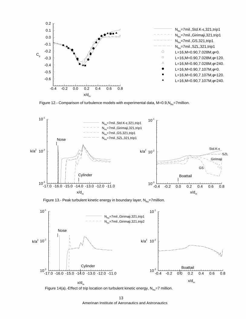
In �gure 12 all the calculations were performed with us-ing a single thin-layer viscous model, i.e., k-thin layer forthis mesh, the min-mod solution limiter, and a turbulenttrip point, trip 1, approximately 0.031 inches (0.08 cm)downstream of the nose. The three ASM predicted a shockstrength slightly weaker than the data and a pressure re-covery slightly lower than the data. The Standard K � "model, in this instance, appears to have better agreementwith the data closely matching peak negative pressure andrecovered to a static pressure only slightly above that of thedata at the boattail trailing edge. Figure 13 is a plot ofthe peak turbulent kinetic energy for each turbulence modelusing the same parameters as the calculations in �gure 12.For clarity, two areas of the axisymmetric body are de-tailed, the region downstream of the nose where the tur-bulent trip occurs and the region around nozzle boattail.The large spike in K=a2 just downstream of x=dm = �16:is the turbulent trip impulse in k. None of the four tur-bulent models tested developed turbulent ow immediatelydownstream of the trip. The Standard K � " linear modeldeveloped turbulence �rst as seen by the rise inK=a2 aroundx=dm = �15:7. The Girimaji and SZL ASM became turbu-lent around x=dm = �15:3, and GS became turbulent thefurthest downstream at x=dm = �14:4.

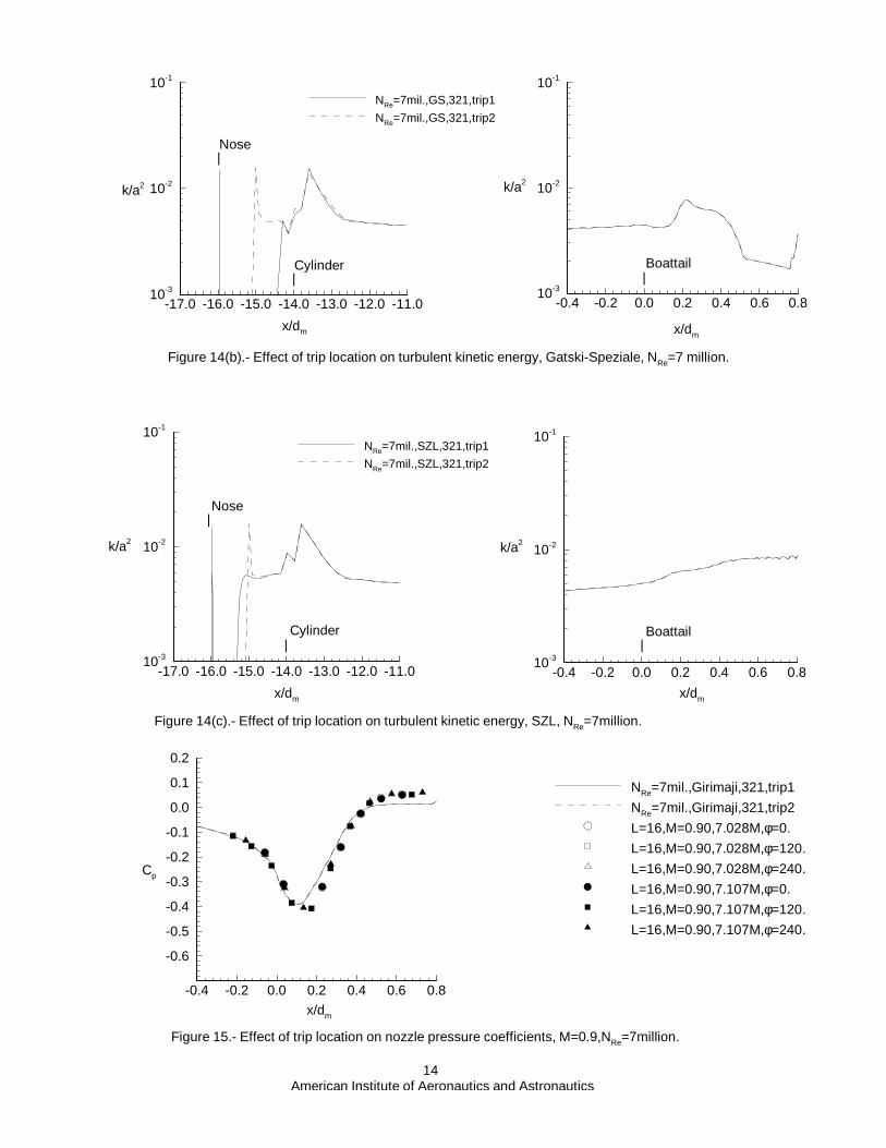
Early studies simulating the incompressible at plate ow displayed similar characteristics. If the turbulenttrip was placed upstream of the critical ow point, tur-bulence would not develop immediately downstream of thetrip. Conversely, turbulence would develop immediatelywhen the turbulent trip was placed downstream of thecritical ow point. Considering this, a di�erent turbu-lent trip point was chosen roughly between the furthestupstream and downstream turbulent development pointsnoted previously and solutions re-developed for the threeASM. Figures 14(a) through (c) show that downstreamof the cone-cylinder transition of body shape, approx.x=dm = �13, despite the di�erent initial development ofturbulence, (trip 1|upstream trip@ x=dm = �15:969 ver-sus trip 2|downstream trip@ x=dm = �15:000) no signif-icant changes occur in the peak turbulent kinetic energy.Figure 15 is representative of the lack of in uence onstatic pressure coe�cient distribution on the nozzle boat-tail between the two turbulent trip points using the min-mod solution limiter. Further parametric studies are neededto determine the boundary layer behavior using other solu-tion limiters with changes in the laminar-to-turbulent owregions.

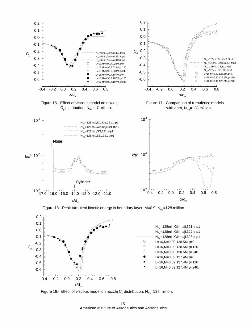
Figure 16 is a study of the e�ect of di�erent viscousmodels on the ow on the afterbody. Three calculationswere performed using k-thin layer (321); j-k viscosity coupled(322); and j-k viscosity uncoupled (323) viscosity modelswith Girimaji ASM at 7 million Reynolds number. Theuse of j-k viscosity appears to improve the comparison withexperimental data by creating a shock slightly stronger andfurther downstream than the k-thin layer calculation, in

addition to slightly raising the pressure recovery in theregion of separated ow. As will be shown subsequently,the observations of best comparison with data will changewith Reynolds number.

High Reynolds number Computations|Figures 17 through21 are high Reynolds number calculations showing the e�ectof turbulence model and viscous model on pressure coe�-cient and turbulent kinetic energy distributions on the body.Figure 17 is a comparison of the four turbulence models atNRe = 128 million using k-thin layer viscosity, min-mod lim-iter and trip1 for turbulent tripping. The three ASM clusteraround the experimental data matching the pressure recov-ery in the separated ow region considerably better than atlow Reynolds numbers. The Standard K � " model predictsthe strongest shock and highest pressure recovery.

Figure 18 is the plot of peak turbulent kinetic energysimilar to �gure 13 for the four turbulence models. Signif-icantly, all four models developed turbulent ow immedi-ately downstream of the turbulent trip as seen by the fourcurves departing from the trip spike inK=a2 at levels around0.004. Each turbulence model remained at slightly di�erentlevels, but had similar trends until the region of ow involv-ing the shock-separation downstream of x=dm = 0:25: Thetrend of the peak turbulent kinetic energy was similar to the7 million Reynolds number trend in �gure 13. Though thethree ASM have very similar static pressure coe�cient dis-tributions, �gure 17, the peak K=a2 trends are completelydi�erent. Also, the Cp distributions between SZL and the

Standard K � "model are very di�erent, but the peak K=a2

have similar trends and levels. Therefore at this point, a cor-relation between the trend of K=a2 and Cp can not be made.

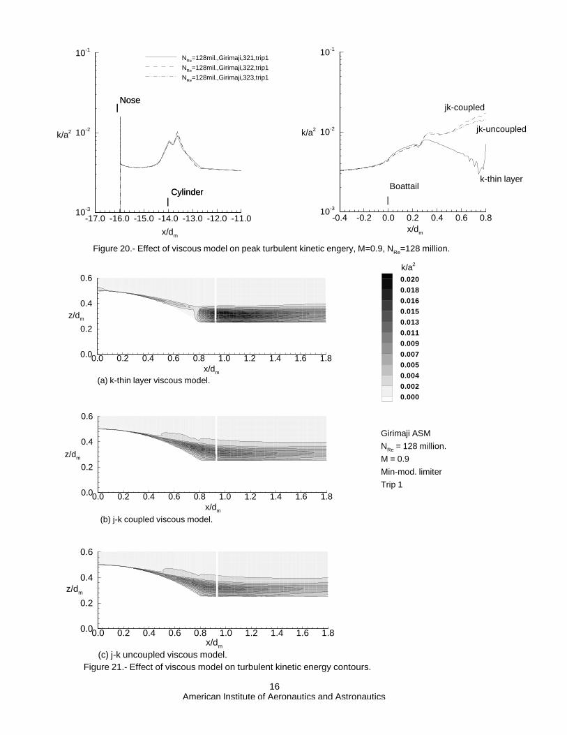
Figure 19 is the e�ect of viscous model using the GirimajiASM at 128 million Reynolds number. In this instance,the k-thin layer calculation (321) provides the best compar-ison with the experimental pressure coe�cient distribution.The j-k viscous models behaved similarly in that the shockstrength increased and the recovery pressure was higher thanthe k-thin layer calculation. Figure 20 is the peak K=a2 forthe three viscous models shown in �gure 19. The three vis-cous models have similar trends in peak turbulent kineticenergy until the region of shock-separated ow downstreamof x=dm = 0:25: Both j-k viscous models generate higherpeak turbulence than the k-thin layer model. The plots in�gures 21(a) to (c) are contours of turbulent kinetic energypredicted by the three viscous models previously discussed.The k-thin layer viscous model, �gure 21(a), has an abruptdiscontinuity in the ow-�eld around the boattail trailingedge, x=dm = :8, while the both j-k viscous models predictvery smooth and continuous contours from the region of theshock, x=dm = :25, to downstream.

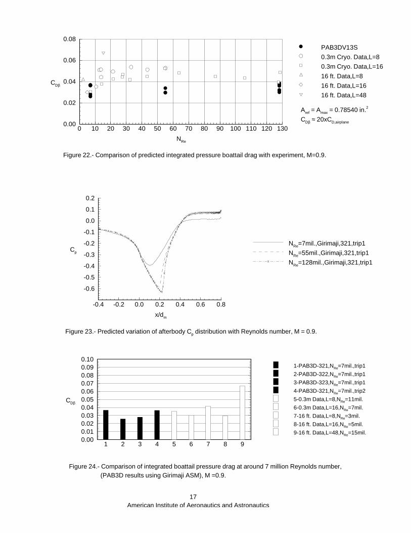
Reynolds number Trends|Figures 22 through 27 aretrends of integrated boattail pressure drag, skin friction, andpredicted point of ow separation with Reynolds number.The integrated pressure drag variation with Reynolds num-ber comparing CFD with experiment is shown in �gure 22.Despite the changes in the shock strength and pressures onthe nozzle boattail with Reynolds number; the variation inpressure drag was small. Overall, the predicted level of pres-sure drag was slightly below that of the experimental data,though at the low and high Reynolds numbers the CFD wasalmost within the scatter of the experimental data. As apoint of reference, 3 additional data points are plotted to

7


include data obtained for the short cryogenic models testedin the 16 Foot Transonic Tunnel at Langley, and the origi-nal 48 inch model also test in the 16 Foot Tunnel.

Figure 23 shows the predicted change in static pressurecoe�cient distribution with Reynolds number. The largestchange seems to occur from the very low Reynolds numberto the mid-range, with the code predicting a large increasein the peak velocity, a downstream shift of the peak and aslight elevation of the static pressure of the ow in the regionof separation. Considerably less change was predicted be-tween the mid-range Reynolds number to the high Reynoldsnumber of 128 million.

Figure 24 is a bar chart of the integrated pressure dragon the boattail at 7 million Reynolds number comparingthe di�erent viscous models and trip location predicted dragwith the Girimaji ASM with experimental data. The higherrecovery pressure that occurred through the j-k viscositycalculations reduced the integrated pressure drag from 37to roughly 28 nozzle drag counts. The scatter in the CFDresults is about the same as the experimental results withthe exception of the 48 inch model data tested in 16-Foot.

High Reynolds number comparisons are shown inFigure 25 with the addition of GS, SZL and Standard K � ".The scatter in the CFD is similar to the low Reynolds num-ber comparison with the Standard K � " predicting the low-est drag due to the considerably higher pressure recovery atthe boattail. Girimaji and SZL, k-thin layer, are the closestto the experimental data, though on the average are low.

Variation of predicted skin friction coe�cients for GirimajiASM with Reynolds number is plotted against at platewetted area estimations in �gure 26. In general, the CFDpredicts skin friction coe�cients are 3.5 nozzle drag countslow at 7 million Reynolds number and about 1.5 nozzle dragcounts low at 128 million Reynolds number. Consideringthe ow e�ects not accounted for by the at plate wet-ted area calculations, (e.g., non-constant Mach number, ad-verse/favorable pressure gradients, aft-projected areas andseparated ow) this comparison is fairly good.

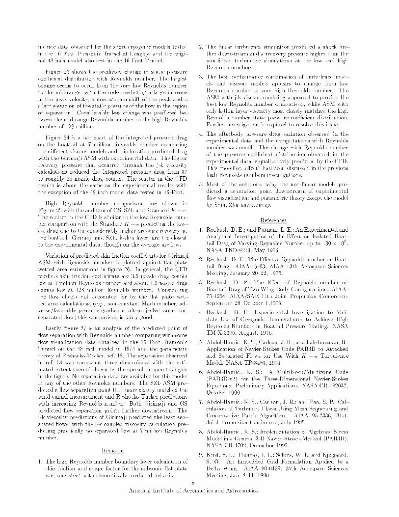
Lastly, �gure 27 is an analysis of the predicted point of ow separation with Reynolds number comparing with some ow visualization data obtained in the 16 Foot TransonicTunnel on the 48 inch model in 1974 and the parametrictheory of Reshotko-Tucker, ref. 18. The separation observedin ref. 18 was somewhat three dimensional with the esti-mated extent thereof shown by the spread in open trianglesin the �gure. No separation data are available for this modelat any of the other Reynolds numbers. The SZL ASM pre-dicted a ow separation point that more closely matched thewind tunnel measurement and Reshotko-Tucker predictionswith increasing Reynolds number. Both Girimaji and GSpredicted ow separation points further downstream. Thej-k viscosity predictions of Girimaji predicted the least sep-arated ows, with the j-k coupled viscosity calculation pre-dicting practically no separated ow at 7 million Reynoldsnumber.

Remarks

1. The high Reynolds number boundary layer calculation ofskin friction and shape factor for the subsonic at platewas consistent with theoretically predicted behavior.

2. The linear turbulence simulation predicted a shock fur-ther downstream and a recovery pressure higher than thenon-linear turbulence simulations at the low and highReynolds numbers.

3. The best performance combination of turbulence mod-els and viscous models appears to change from lowReynolds number to very high Reynolds number. TheASM with j-k viscous modeling appeared to provide thebest low Reynolds number comparison, while ASM withonly k-thin layer viscosity most closely matched the highReynolds number static pressure coe�cient distribution.Further investigation is required to resolve this issue.

4. The afterbody pressure drag variation observed in theexperimental data and the computations with Reynoldsnumber was small. The change with Reynolds numberof the pressure coe�cient distribution observed in theexperimental data is qualitatively predicted by the CFD.This \no-e�ect e�ect" had been discussed in the previoushigh Reynolds numbers investigations.

5. Most of the solutions using the non-linear models pre-dicted a separation point downstream of experimental ow visualization and parametric theory except the modelby Shih, Zhu and Lumley.

References

1. Reubush, D. E.; and Putnam, L. E.: An Experimental andAnalytical Investigation of the E�ect on Isolated Boat-tail Drag of Varying Reynolds Number up to 130 � 106.NASA TND-8210, May 1976.

2. Reubush, D. E.: The E�ect of Reynolds number on Boat-tail Drag. AIAA-75-63, AIAA 13th Aerospace SciencesMeeting, January 20{22, 1975.

3. Reubush, D. E.: The E�ect of Reynolds number onBoattail Drag of Two Wing-Body Con�gurations. AIAA-75-1294, AIAA/SAE 11th Joint Propulsion Conference,September 29{October 1,1975.

4. Reubush, D. E.: Experimental Investigation to Vali-date Use of Cryogenic Temperatures to Achieve HighReynolds Numbers in Boattail Pressure Testing. NASATM X-3396, August, 1976.

5. Abdol-Hamid, K. S.; Carlson, J. R.; and Lakshmanan, B.:Application of Navier-Stokes Code PAB3D to Attachedand Separated Flows for Use With K � � TurbulenceModel. NASA TP-3480, 1994.

6. Abdol-Hamid, K. S.: A Multiblock/Multizone Code(PAB3D-v2) for the Three-Dimensional Navier-StokesEquations: Preliminary Applications. NASA CR-182032,October 1990.

7. Abdol-Hamid, K. S.; Carlson, J. R.; and Pao, S. P.: Cal-culation of Turbulent Flows Using Mesh Sequencing andConservative Patch Algorithm. AIAA 95-2336, 31st.Joint Propulsion Conference, July 1995.

8. Abdol-Hamid, K. S.: Implementation of Algebraic StressModel in a General 3-D Navier-Stokes Method (PAB3D).NASA CR-4702, December 1995.

9. Krist, S. L.; Thomas, J. L.; Sellers, W. L; and Kjelgaard,S. O.: An Embedded Grid Formulation Applied to aDelta Wing. AIAA 90-0429, 28th Aerospace SciencesMeeting, Jan. 8{11, 1990.

8


10. Patel, V. C.; Rodi, W.; and Scheuerer G.: TurbulenceModels for Near-Wall and Low Reynolds Number Flows:A Review. AIAA Journal, Vol. 23, No. 9, pp. 1308{1319,September 1985.

11. Launder, B. E. and Sharma, B. I.: Application of the En-ergy Dissipation Model of Turbulence to the Calculationof Flow Near a Spinning Disk. Letters in Heat and MassTransfer, Vol. 1, 1974, pp. 131{138.

12. Shih, T-H; Zhu, J.; and Lumley, J. L.: A NewReynolds Stress Algebraic Model. NASA TM-166644,ICOMP 94-8, 1994.

13. Gatski, T. B. and Speziale, C. G.: On Explicit AlgebraicStress Models for Complex Turbulent Flows. NASACR-189725, ICASE Report No. 92-58, November 1992.

14. Girimaji, S. S.: Fully-explicit and Self-consistent alge-braic Reynolds Stress Model. ICASE Report 95-82, 1995.

15. Spalart, P. R.: Direct Simulations of Turbulent BoundaryLayers up to Re

�= 1420: Journal of Fluid Mechanics,

Vol. 187, pp. 61{98, 1988.

16. Kilgore, R. A.; Adcock, J. B.; and Edward, J.: FlightSimulation Characteristics of the Langley High ReynoldsNumber Cryogenic Transonic Tunnel. AIAA 74-80, Jan.1974.

17. Cahn, M. S.: An Experimental Investigation of Sting-Support E�ects on Drag and a Comparison With JetE�ects at Transonic Speeds. NACA Report 1353, 1958.

18. Abeyounis, W. K.: Boundary-Layer Separation on Iso-lated Boattail Nozzles. NASA TP-1226, August 1978.

Appendix

The functions and variables used in the Girimaji algebraicReynolds stress model are listed:

L01=

C01

2� 1;L1

1= C1

1+ 2

L2 =C2

2�

2

3; L3 =

C2

2� 1; L4 =

C4

2� 1:

�1 =

�K

�

�2

SmnSmn; �2 =

�K

�

�2

WmnWmn

p = �2L0

1

�1L11

; r = �L01L2�

�1L11

�2

q =1

(�1L11)2

��L01

�2+ �1L

11L2 �

2

3�1 (L3)

2 + 2�2 (L4)2

�

a =

�q �

p2

3

�; b =

1

27

�2p3 � 9pq + 27r

�

D =b2

4+a3

27; cos(�) =

�b=2p�a3=27

The coe�cients G2 and G3 are:

G2 =�L4G1

L10� �1L

11G1

; G3 =2L3G1

L10� �1L

11G1

additionally

C01= 3:4; C1

1= 1:8; C2 = 0:36; C3 = 1:25; C4 = 0:4:

9


10-1 100 101 102 1030.0

0.2

0.4

0.6

0.8

1.0

-u’v’+

y+

(b) Turbulent shear stress at Rθ=1420.

-1 0 1 2 3 4 50.0

0.5

1.0

1.5

2.0

B1 81x121

B2 81x121

B3 81x121

B3B2B1

M=0.097

pt0 = 1.7229MPa

Inflowboundary

l.e. x(m)

Figure 1.-Block and grid arrangement for subsonic flat plate.

10-5 10-4 10-3 10-2 10-1 100 101102

103

104

105

106

107

108

109

Figure 2.-Reynolds number with distance along flat plate.x(m)

Rx

10-1 100 101 102 1030

5

10

15

20

25

u+

y+

Figure 3.- Comparison of boundary layer characteristics for different turbulence models.

(a) Law-of-the-wall profile at Rθ=1420.

10

American Institute of Aeronautics and Astronautics

0.35 Girimaji

0.32 GS

κ ASM

0.28 SZL

0.39 DNS

Girimaji ASM

Gatski-Speziale ASM

Shih,Zhu & Lumley ASM

DNS

10-1 100 101 102 103 104 1050.0

0.2

0.4

0.6

0.8

1.0

1.2

-u’v’+

y+

(b) Turbulent shear stress at Rθ=100,000.

104 105 106 107 108 1090.001

0.002

0.003

0.004

0.0050.0060.0070.0080.009

0.01

Rx

cf

Figure 5.-Local skin friction for subsonic flat plate.

Girimaji ASM

Gatski-Speziale ASM

Shih, Zhu & Lumley

Blasius solution

Transition region

1/5th Power solution

White-Exact theory

104 105 106 107 108 1090.001

0.002

0.003

0.004

0.0050.0060.0070.0080.009

0.01

American Institute of Aeronautics and Astronautics11

RL

CF

Figure 6.-Average skin friction for subsonic flat plate, (same symbol table as figure 5).

10-1 100 101 102 103 104 1050

5

10

15

20

25

30

35

u+

y+

(a) Law-of-the-wall profile at Rθ=100,000.

Figure 4.- Comparison of boundary layer characteristics for different turbulence models.

0.44 Girimaji

0.38 GS

0.34 SZL

0.40 Turb.

0.48 Turb-2

κ ASM

Girimaji ASM

Gatski-Speziale ASM

Shih,Zhu & Lumley

Laminar Sublayer

Buffer Region

Turbulent Region

Turbulent Region-2

-0.4 -0.2 0.0 0.2 0.4 0.6 0.8

-0.6

-0.5

-0.4

-0.3

-0.2

-0.1

0.0

0.1

0.2

Cp

Figure 11.- Representative grid sensitivity at

x/dm

128 million Reynolds number.

NRe=128mil.,Girimaji,144-321,t



L=16,M=0.90,128.5M,φ=0.

L=16,M=0.90,128.5M,φ=120.

L=16,M=0.90,128.5M,φ=240.

L=16,M=0.89,127.4M,φ=0.

L=16,M=0.89,127.4M,φ=120.

L=16,M=0.89,127.4M,φ=240.

102 103 104 105 10610-1

100

101

102

103

µτ/µ

Rδ1

Figure 7.- Turbulent viscosity developmentwith Rδ1

Girimaji ASM

Gatski-Speziale ASM

Shih, Zhu & Lumley

102 103 104 105 106 107 108 1090.5

1.0

1.5

2.0

2.5

3.0

Rx

H12

Figure 8.- Boundary layer shape factor developmentwith Rx

Girimaji ASM

Gatski-Speziale ASM

Shih, Zhu & Lumley

Flat plate theory

Figure 9.- Photograph of 8 inch model in 0.3m Transonic Cryogenic Tunnel.

-0.4 -0.2 0.0 0.2 0.4 0.6 0.8

-0.6

-0.5

-0.4

-0.3

-0.2

-0.1

0.0

0.1

0.2


Cp

x/dm

Figure 10.- Representative grid sensitivity at7 million Reynolds number.

NRe=7mil.,Girimaji,144-321,tri



L=16,M=0.90,7.028M,φ=0.

L=16,M=0.90,7.028M,φ=120.

L=16,M=0.90,7.028M,φ=240.

L=16,M=0.90,7.107M,φ=0.

L=16,M=0.90,7.107M,φ=120.

L=16,M=0.90,7.107M,φ=240.

-17.0 -16.0 -15.0 -14.0 -13.0 -12.0 -11.010-3

10-2

10-1

|Cylinder

|Nose

k/a2

x/dm

Figure 13.- Peak turbulent kinetic energy in boundary layer, NRe=7million.

-0.4 -0.2 0.0 0.2 0.4 0.6 0.810-3

10-2

10-1

Boattail|

k/a2

x/dm

NRe=7mil.,Girimaji,321,trip1


-0.4 -0.2 0.0 0.2 0.4 0.6 0.8

-0.6

-0.5

-0.4

-0.3

-0.2

-0.1

0.0

0.1

0.2

Cp

x/dm

Figure 12.- Comparison of turbulence models with experimental data, M=0.9,NRe=7million.

NRe=7mil.,Std.K-ε,321,trip1


NRe=7mil.,GS,321,trip1

NRe=7mil.,SZL,321,trip1

L=16,M=0.90,7.028M,φ=0.

L=16,M=0.90,7.028M,φ=120.

L=16,M=0.90,7.028M,φ=240.

L=16,M=0.90,7.107M,φ=0.

L=16,M=0.90,7.107M,φ=120.

L=16,M=0.90,7.107M,φ=240.

-0.4 -0.2 0.0 0.2 0.4 0.6 0.810-3

10-2

10-1

k/a2

x/dm

Boattail|

Girimaji

SZL

Std.K-ε

GS





-17.0 -16.0 -15.0 -14.0 -13.0 -12.0 -11.010-3

10-2

10-1

|Cylinder

|Nose

k/a2

x/dm

Amerinan Institute of Aeronautics and Astronautics13

Figure 14(a).-Effect of trip location on turbulent kinetic energy, NRe=7 million.

-0.4 -0.2 0.0 0.2 0.4 0.6 0.810-3

10-2

10-1

k/a2

x/dm

|Boattail



-0.4 -0.2 0.0 0.2 0.4 0.6 0.810-3

10-2

10-1

x/dm

k/a2

Boattail|



-17.0 -16.0 -15.0 -14.0 -13.0 -12.0 -11.010-3

10-2

10-1

k/a2

|Cylinder

|Nose

x/dm

Figure 14(b).- Effect of trip location on turbulent kinetic energy, Gatski-Speziale, NRe=7 million.

-17.0 -16.0 -15.0 -14.0 -13.0 -12.0 -11.010-3

10-2

10-1

k/a2

x/dm

|Nose

|Cylinder

Figure 14(c).- Effect of trip location on turbulent kinetic energy, SZL, NRe=7million.

-0.4 -0.2 0.0 0.2 0.4 0.6 0.8

-0.6

-0.5

-0.4

-0.3

-0.2

-0.1

0.0

0.1

0.2

Cp

x/dm


Figure 15.- Effect of trip location on nozzle pressure coefficients, M=0.9,NRe=7million.



L=16,M=0.90,7.028M,φ=0.

L=16,M=0.90,7.028M,φ=120.

L=16,M=0.90,7.028M,φ=240.

L=16,M=0.90,7.107M,φ=0.

L=16,M=0.90,7.107M,φ=120.

L=16,M=0.90,7.107M,φ=240.

-0.4 -0.2 0.0 0.2 0.4 0.6 0.810-3

10-2

10-1

Cylinder|

|Nose

k/a2

x/dm

-0.4 -0.2 0.0 0.2 0.4 0.6 0.8

-0.6

-0.5

-0.4

-0.3

-0.2

-0.1

0.0

0.1

0.2

Cp

x/dm

Figure 17.- Comparison of turbulence modelswith data, NRe=128 million.





L=16,M=0.90,128.5M,φ=0.

L=16,M=0.90,128.5M,φ=120.

L=16,M=0.90,128.5M,φ=240.

-17.0 -16.0 -15.0 -14.0 -13.0 -12.0 -11.010-3

10-2

10-1

Cylinder|

|Nose

x/dm

k/a2

Figure 18.- Peak turbulent kinetic energy in boundary layer, M=0.9, NRe=128 million.





-0.4 -0.2 0.0 0.2 0.4 0.6 0.8

-0.6

-0.5

-0.4

-0.3

-0.2

-0.1

0.0

0.1

0.2

x/dm

Cp

Figure 16.- Effect of viscous model on nozzleCp distribution, NRe = 7 million.




L=16,M=0.90,7.028M,φ=0.

L=16,M=0.90,7.028M,φ=120.

L=16,M=0.90,7.028M,φ=240.

L=16,M=0.90,7.107M,φ=0.

L=16,M=0.90,7.107M,φ=120.

L=16,M=0.90,7.107M,φ=240.

-0.4 -0.2 0.0 0.2 0.4 0.6 0.8

-0.6

-0.5

-0.4

-0.3

-0.2

-0.1

0.0

0.1

0.2

x/dm

Cp


Figure 19.- Effect of viscous model on nozzle Cp distribution, NRe=128 million.




L=16,M=0.90,128.5M,φ=0.

L=16,M=0.90,128.5M,φ=120.

L=16,M=0.90,128.5M,φ=240.

L=16,M=0.89,127.4M,φ=0.

L=16,M=0.89,127.4M,φ=120.

L=16,M=0.89,127.4M,φ=240.

-17.0 -16.0 -15.0 -14.0 -13.0 -12.0 -11.010-3

10-2

10-1

Cylinder|

|Nose

k/a2

Figure 20.- Effect of viscous model on peak turbulent kinetic engery, M=0.9, NRe=128 million.

x/dm




-0.4 -0.2 0.0 0.2 0.4 0.6 0.810-3

10-2

10-1

Cylinder|

|Nose

k/a2

x/dm

|

Boattailk-thin layer

jk-coupled

jk-uncoupled

0.0 0.2 0.4 0.6 0.8 1.0 1.2 1.4 1.6 1.80.0

0.2

0.4

0.6


x/dm

z/dm

(c) j-k uncoupled viscous model.Figure 21.- Effect of viscous model on turbulent kinetic energy contours.

0.0 0.2 0.4 0.6 0.8 1.0 1.2 1.4 1.6 1.80.0

0.2

0.4

0.6

Girimaji ASM

NRe = 128 million.

M = 0.9

Min-mod. limiter

Trip 1

x/dm

z/dm

(b) j-k coupled viscous model.

0.0 0.2 0.4 0.6 0.8 1.0 1.2 1.4 1.6 1.80.0

0.2

0.4

0.6

z/dm

x/dm

k/a2

(a) k-thin layer viscous model.

0.020

0.018

0.016

0.015

0.013

0.011

0.009

0.007

0.005

0.004

0.002

0.000

-0.4 -0.2 0.0 0.2 0.4 0.6 0.8

-0.6

-0.5

-0.4

-0.3

-0.2

-0.1

0.0

0.1

0.2

Cp

x/dm

Figure 23.- Predicted variation of afterbody Cp distribution with Reynolds number, M = 0.9.




1 2 3 4 5 6 7 8 90.000.010.020.030.040.050.060.070.080.090.10


CDβ

Figure 24.- Comparison of integrated boattail pressure drag at around 7 million Reynolds number,(PAB3D results using Girimaji ASM), M =0.9.

1-PAB3D-321,NRe=7mil.,trip1




5-0.3m Data,L=8,NRe=11mil.

6-0.3m Data,L=16,NRe=7mil.

7-16 ft. Data,L=8,NRe=3mil.



0 10 20 30 40 50 60 70 80 90 100 110 120 1300.00

0.02

0.04

0.06

0.08

CDβ

NRe

Figure 22.- Comparison of predicted integrated pressure boattail drag with experiment, M=0.9.

Aref = Amax = 0.78540 in.2

CDβ ≈ 20xCD,airplane

PAB3DV13S

0.3m Cryo. Data,L=8

0.3m Cryo. Data,L=16

16 ft. Data,L=8

16 ft. Data,L=16

16 ft. Data,L=48

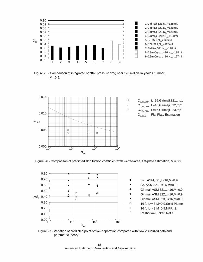
1 2 3 4 5 6 7 8 90.000.010.020.030.040.050.060.070.080.090.10

CDβ

Figure 25.- Comparison of integrated boattail pressure drag near 128 million Reynolds number,M =0.9.

1-Girimaji-321,NRe=128mil.



4-Girimaji-321z,NRe=128mil.

5-GS-321,NRe=128mil.

6-SZL-321,NRe=128mil.

7-Std.K-ε,321,NRe=128mil.

8-0.3m Cryo.,L=16,NRe=128mil.

9-0.3m Cryo.,L=16,NRe=127mil.

106 107 108 1090.000

0.005

0.010

0.015

CD,β,sf

NRe

Figure 26.- Comparison of predicted skin friction coefficient with wetted-area, flat-plate estimation, M = 0.9.

CD,βsf,CFD L=16,Girimaji,321,trip1



CD,βsf,fp Flat Plate Estimation

106 107 108 1090.00

0.10

0.20

0.30

0.40

0.50

0.60

0.70

0.80

x/dm

NRe


Figure 27.- Variation of predicted point of flow separation compared with flow visualized data and parametric theory.

SZL ASM,321,L=16,M=0.9

GS ASM,321,L=16,M=0.9

Girimaji ASM,321,L=16,M=0.9



16 ft.,L=48,M=0.9,Solid Plume

16 ft.,L=48,M=0.9,NPR=2.

Reshotko-Tucker, Ref.18

Documents

HIGH REYNOLDS NUMBER ANALYSIS OF FLAT …mln/ltrs-pdfs/NASA-aiaa-96-2544.pdfhigh reynolds number analysis of flat plate and separated afterbody flow using non-linear turbulence models