Embed Size (px)
Citation preview

Herd Management Science
Preliminary editionCompiled for the Advanced Herd Management course
KVL, August 28th - November 3rd, 2006
Anders Ringgaard KristensenErik Jørgensen
Nils ToftThe Royal Veterinary and Agricultural University
Copenhagen, Denmark

2

3
PrefaceIn 1996 two of the authors organized a Nordic PhD course on Planning and Con-trol of Animal Production at Farm Level. The third author, Nils Toft, attended thecourse as a PhD student. As part of the material for the course, 5 textbook noteswere written and published as Dina Notes.
The notes were successfully used at the course in 1996, and afterwards theyhave served as important input to the Master level course on Advanced Herd Man-agement given at the Royal Veterinary and Agricultural University. A couple of thenotes have been slightly updated over the years, but basically the content has notchanged.
Over the years, the authors have had the wish to collect and update the materialin order to create an authoritative textbook covering more or less all aspects of herdmanagement from the basic to the advanced level. This preliminary edition is thefirst attempt to realize this wish. Even though there is still a long way to go beforethe work is done, it is our hope that the preliminary version will turn out to beuseful for the participants of the Advanced Herd Management course held at KVLin 2006.
The book is organized in two parts with basic herd management principles andclassical theories in part I, and the more advanced methods in part II. Furthermore,the necessary mathematical and statistical theory is summarized in appendices foreasy reference.
Part I has been written with a bachelor level course in mind, and the contentsreflect what we think that any animal scientist should master, whereas Part II hasbeen written for a more advanced level for graduate students who wish to special-ize in Herd Management. Given the structural development in modern agriculturewith ever increasing herd sizes, we expect that the need for an advanced textbookfocusing directly on herd management will increase.
Copenhagen, August 2006
Anders Ringgaard KristensenErik Jørgensen
Nils Toft

4
This book has a home page at URL: http://www.dina.dk/∼ark/book.htm

Contents
I Basic concepts 15
1 Introduction 171.1 Definition of herd management science . . . . . . . . . . . . . . 171.2 The herd management problem . . . . . . . . . . . . . . . . . . . 211.3 The management cycle . . . . . . . . . . . . . . . . . . . . . . . 23
1.3.1 The elements of the cycle . . . . . . . . . . . . . . . . . 231.3.2 Production monitoring and decision making . . . . . . . . 261.3.3 Levels . . . . . . . . . . . . . . . . . . . . . . . . . . . . 271.3.4 Time horizons . . . . . . . . . . . . . . . . . . . . . . . 27
2 The role of models in herd management 292.1 The decision making process . . . . . . . . . . . . . . . . . . . . 292.2 Why models? . . . . . . . . . . . . . . . . . . . . . . . . . . . . 302.3 Knowledge representation . . . . . . . . . . . . . . . . . . . . . 32
2.3.1 The current state of the unit . . . . . . . . . . . . . . . . 322.3.2 The production function . . . . . . . . . . . . . . . . . . 342.3.3 Other kinds of knowledge . . . . . . . . . . . . . . . . . 352.3.4 Knowledge acquisition as a decision . . . . . . . . . . . . 36
3 Objectives of production: Farmer’s preferences 373.1 Attributes of the utility function . . . . . . . . . . . . . . . . . . 373.2 Common attributes of farmers’ utility functions . . . . . . . . . . 38
3.2.1 Monetary gain . . . . . . . . . . . . . . . . . . . . . . . 383.2.2 Leisure time . . . . . . . . . . . . . . . . . . . . . . . . 393.2.3 Animal welfare . . . . . . . . . . . . . . . . . . . . . . . 393.2.4 Working conditions . . . . . . . . . . . . . . . . . . . . . 423.2.5 Environmental preservation . . . . . . . . . . . . . . . . 433.2.6 Personal prestige . . . . . . . . . . . . . . . . . . . . . . 433.2.7 Product quality . . . . . . . . . . . . . . . . . . . . . . . 44
3.3 From attributes to utility . . . . . . . . . . . . . . . . . . . . . . 443.3.1 Aggregation of attributes, uncertainty . . . . . . . . . . . 443.3.2 Single attribute situation: Risk . . . . . . . . . . . . . . . 443.3.3 Multiple attribute situation . . . . . . . . . . . . . . . . . 48

6 CONTENTS
3.3.4 Operational representation of a farmer’s utility function . . 52
4 Classical production theory 554.1 One to one relations . . . . . . . . . . . . . . . . . . . . . . . . . 55
4.1.1 The production function . . . . . . . . . . . . . . . . . . 554.1.2 What to produce . . . . . . . . . . . . . . . . . . . . . . 564.1.3 How to produce . . . . . . . . . . . . . . . . . . . . . . . 584.1.4 How much to produce . . . . . . . . . . . . . . . . . . . 60
4.2 Multi-dimensional production models . . . . . . . . . . . . . . . 624.3 Limitations of the neo-classical production theory . . . . . . . . . 634.4 Costs . . . . . . . . . . . . . . . . . . . . . . . . . . . . . . . . 63
4.4.1 Variable costs and fixed costs: Gross margins . . . . . . . 634.4.2 Opportunity costs and internal prices . . . . . . . . . . . 644.4.3 Investments . . . . . . . . . . . . . . . . . . . . . . . . . 67
4.5 Other classical techniques . . . . . . . . . . . . . . . . . . . . . . 684.5.1 Partial budgeting . . . . . . . . . . . . . . . . . . . . . . 684.5.2 Cost-benefit analysis . . . . . . . . . . . . . . . . . . . . 694.5.3 Decision tree analysis . . . . . . . . . . . . . . . . . . . 70
4.6 Classical replacement theory . . . . . . . . . . . . . . . . . . . . 724.6.1 Replacement with identical assets . . . . . . . . . . . . . 724.6.2 Optimal replacement using discounting . . . . . . . . . . 744.6.3 Technological or genetical improvement . . . . . . . . . . 754.6.4 Limitations and applications of the classical replacement
theory . . . . . . . . . . . . . . . . . . . . . . . . . . . . 774.7 Exercises . . . . . . . . . . . . . . . . . . . . . . . . . . . . . . 79
4.7.1 Gross margin . . . . . . . . . . . . . . . . . . . . . . . . 794.7.2 Internal prices . . . . . . . . . . . . . . . . . . . . . . . . 804.7.3 Marginal considerations, I . . . . . . . . . . . . . . . . . 814.7.4 Marginal considerations, II . . . . . . . . . . . . . . . . . 824.7.5 Investments . . . . . . . . . . . . . . . . . . . . . . . . . 82
5 Basic production monitoring 835.1 The framework . . . . . . . . . . . . . . . . . . . . . . . . . . . 835.2 The elements of the monitoring process . . . . . . . . . . . . . . 85
5.2.1 Data recording . . . . . . . . . . . . . . . . . . . . . . . 855.2.2 Database . . . . . . . . . . . . . . . . . . . . . . . . . . 865.2.3 Data processing . . . . . . . . . . . . . . . . . . . . . . . 875.2.4 Report with key figures . . . . . . . . . . . . . . . . . . . 89
Types of key figures . . . . . . . . . . . . . . . . . . . . 89Key figures and their interrelations . . . . . . . . . . . . . 90Properties of key figures . . . . . . . . . . . . . . . . . . 92Correctness . . . . . . . . . . . . . . . . . . . . . . . . . 93Validity . . . . . . . . . . . . . . . . . . . . . . . . . . . 94Precision . . . . . . . . . . . . . . . . . . . . . . . . . . 96

CONTENTS 7
5.2.5 Analysis from a statistical point of view . . . . . . . . . . 97General principles . . . . . . . . . . . . . . . . . . . . . 97Continuous properties . . . . . . . . . . . . . . . . . . . 98Categorical properties without observation error . . . . . . 102Categorical properties with observation error . . . . . . . 104Concluding remarks . . . . . . . . . . . . . . . . . . . . 108
5.2.6 Analysis from a utility point of view . . . . . . . . . . . . 1085.2.7 Decision: Adjustment/no adjustment . . . . . . . . . . . . 111
When to adjust . . . . . . . . . . . . . . . . . . . . . . . 111Where to adjust . . . . . . . . . . . . . . . . . . . . . . . 111How to adjust . . . . . . . . . . . . . . . . . . . . . . . . 111
5.3 Exercises . . . . . . . . . . . . . . . . . . . . . . . . . . . . . . 1125.3.1 Milk yield . . . . . . . . . . . . . . . . . . . . . . . . . . 1125.3.2 Daily gain in slaughter pigs . . . . . . . . . . . . . . . . 112
Valuation weighings . . . . . . . . . . . . . . . . . . . . 112Individual gains . . . . . . . . . . . . . . . . . . . . . . . 113First in - first out . . . . . . . . . . . . . . . . . . . . . . 113Comparison of methods . . . . . . . . . . . . . . . . . . 113Numerical example . . . . . . . . . . . . . . . . . . . . . 114
5.3.3 Reproduction in dairy herds . . . . . . . . . . . . . . . . 1155.3.4 Disease treatments . . . . . . . . . . . . . . . . . . . . . 1165.3.5 Validity, reproduction . . . . . . . . . . . . . . . . . . . . 1175.3.6 Economic significance of days open . . . . . . . . . . . . 117
II Advanced topics 119
6 From registration to information 1216.1 Information as a production factor . . . . . . . . . . . . . . . . . 1216.2 Data sources: examples . . . . . . . . . . . . . . . . . . . . . . . 122
6.2.1 The heat detection problem . . . . . . . . . . . . . . . . . 1226.2.2 The weighing problem . . . . . . . . . . . . . . . . . . . 1226.2.3 The activity problem . . . . . . . . . . . . . . . . . . . . 1236.2.4 Miscellaneous . . . . . . . . . . . . . . . . . . . . . . . 123
6.3 Basic concepts and definitions . . . . . . . . . . . . . . . . . . . 1236.3.1 Utility value of registrations . . . . . . . . . . . . . . . . 1246.3.2 Entropy based value . . . . . . . . . . . . . . . . . . . . 127
6.4 Measurement errors . . . . . . . . . . . . . . . . . . . . . . . . . 1276.4.1 Registration failure . . . . . . . . . . . . . . . . . . . . . 1276.4.2 Measurement precision . . . . . . . . . . . . . . . . . . . 1286.4.3 Indirect measure . . . . . . . . . . . . . . . . . . . . . . 1286.4.4 Bias . . . . . . . . . . . . . . . . . . . . . . . . . . . . . 1296.4.5 Rounding errors . . . . . . . . . . . . . . . . . . . . . . 1306.4.6 Interval censoring . . . . . . . . . . . . . . . . . . . . . . 130

8 CONTENTS
6.4.7 Categorical measurements . . . . . . . . . . . . . . . . . 1306.4.8 Enhanced models of categorical measurements . . . . . . 1336.4.9 Pre selection . . . . . . . . . . . . . . . . . . . . . . . . 1346.4.10 Registration of interventions . . . . . . . . . . . . . . . . 1346.4.11 Missing registrations . . . . . . . . . . . . . . . . . . . . 1356.4.12 Selection and censoring . . . . . . . . . . . . . . . . . . 1356.4.13 Discussion . . . . . . . . . . . . . . . . . . . . . . . . . 137
6.5 Data processing . . . . . . . . . . . . . . . . . . . . . . . . . . . 1376.5.1 Threshold level . . . . . . . . . . . . . . . . . . . . . . . 1386.5.2 Change point estimation . . . . . . . . . . . . . . . . . . 1396.5.3 Significance test in experiments . . . . . . . . . . . . . . 139
6.6 Utility evaluation examples . . . . . . . . . . . . . . . . . . . . . 1406.6.1 Production control . . . . . . . . . . . . . . . . . . . . . 1406.6.2 Recording of sow specific litter size . . . . . . . . . . . . 1426.6.3 Precision in weighing of slaughter pigs . . . . . . . . . . 144
6.7 Outlook . . . . . . . . . . . . . . . . . . . . . . . . . . . . . . . 146
7 Dynamic production monitoring by classical methods 147
8 Dynamic production monitoring by state space models 149
9 Decisions and strategies: A survey of methods 1519.1 Framework of the survey . . . . . . . . . . . . . . . . . . . . . . 1519.2 Rule based expert systems . . . . . . . . . . . . . . . . . . . . . 1519.3 Linear programming with extensions . . . . . . . . . . . . . . . . 1539.4 Dynamic programming and Markov decision processes . . . . . . 1559.5 Probabilistic Expert systems: Bayesian networks . . . . . . . . . 1589.6 Decision graphs . . . . . . . . . . . . . . . . . . . . . . . . . . . 1599.7 Simulation . . . . . . . . . . . . . . . . . . . . . . . . . . . . . . 161
10 Modeling and sensitivity analysis by Linear Programming 16710.1 Introduction . . . . . . . . . . . . . . . . . . . . . . . . . . . . . 167
10.1.1 Phases of modeling . . . . . . . . . . . . . . . . . . . . . 16710.1.2 Formulating the problem . . . . . . . . . . . . . . . . . . 16810.1.3 Constructing a Mathematical Model . . . . . . . . . . . . 16810.1.4 Deriving a solution . . . . . . . . . . . . . . . . . . . . . 16910.1.5 Testing the model and the solution . . . . . . . . . . . . . 16910.1.6 Establishing control over the solution . . . . . . . . . . . 16910.1.7 Implementation . . . . . . . . . . . . . . . . . . . . . . . 170
10.2 Using linear programming . . . . . . . . . . . . . . . . . . . . . 17010.2.1 The model setup . . . . . . . . . . . . . . . . . . . . . . 17010.2.2 Proportionality . . . . . . . . . . . . . . . . . . . . . . . 17010.2.3 Additivity . . . . . . . . . . . . . . . . . . . . . . . . . . 17110.2.4 Divisibility . . . . . . . . . . . . . . . . . . . . . . . . . 171

CONTENTS 9
10.2.5 Certainty . . . . . . . . . . . . . . . . . . . . . . . . . . 17110.2.6 Circumventing the assumptions . . . . . . . . . . . . . . 17110.2.7 Construction of constraints . . . . . . . . . . . . . . . . . 17210.2.8 Natural extensions of the LP-model . . . . . . . . . . . . 174
10.3 Sensitivity analysis . . . . . . . . . . . . . . . . . . . . . . . . . 17510.3.1 Shadow prices . . . . . . . . . . . . . . . . . . . . . . . 17510.3.2 Price adjustments . . . . . . . . . . . . . . . . . . . . . . 17710.3.3 Capacity changes . . . . . . . . . . . . . . . . . . . . . . 17810.3.4 Additional constraints . . . . . . . . . . . . . . . . . . . 178
10.4 Concluding remarks . . . . . . . . . . . . . . . . . . . . . . . . . 18010.5 Exercise . . . . . . . . . . . . . . . . . . . . . . . . . . . . . . . 180
11 Bayesian networks 183
12 Decision graphs: Potential use and current limitations 18512.1 Introduction . . . . . . . . . . . . . . . . . . . . . . . . . . . . . 18512.2 From decision tree to influence diagram . . . . . . . . . . . . . . 18612.3 From Bayesian network to influence diagram . . . . . . . . . . . 18712.4 From Dynamic Programming to influence diagrams . . . . . . . . 18812.5 Examples . . . . . . . . . . . . . . . . . . . . . . . . . . . . . . 190
12.5.1 The two-sow problem . . . . . . . . . . . . . . . . . . . 19012.5.2 The registration problem for the whole cycle . . . . . . . 19112.5.3 The repeated measurement problem . . . . . . . . . . . . 19412.5.4 Optimal timing of matings . . . . . . . . . . . . . . . . . 19512.5.5 The feed analysis problem . . . . . . . . . . . . . . . . . 196
12.6 Outlook . . . . . . . . . . . . . . . . . . . . . . . . . . . . . . . 198
13 Dynamic programming and Markov decision processes 19913.1 Introduction . . . . . . . . . . . . . . . . . . . . . . . . . . . . . 199
13.1.1 Historical development . . . . . . . . . . . . . . . . . . . 19913.1.2 Applications in animal production . . . . . . . . . . . . . 201
13.2 Variability and cyclic production: Markov decision programming 20213.2.1 Notation and terminology . . . . . . . . . . . . . . . . . 20313.2.2 A simple dairy cow replacement model . . . . . . . . . . 20313.2.3 Criteria of optimality . . . . . . . . . . . . . . . . . . . 205
Finite planning horizon . . . . . . . . . . . . . . . . . . . 205Infinite planning horizon . . . . . . . . . . . . . . . . . . 205
13.2.4 Optimization techniques in general Markov decision pro-gramming . . . . . . . . . . . . . . . . . . . . . . . . . 207Value iteration . . . . . . . . . . . . . . . . . . . . . . . 207The simple dairy model optimized by value iteration . . . 208Policy iteration . . . . . . . . . . . . . . . . . . . . . . . 211Linear programming . . . . . . . . . . . . . . . . . . . . 212
13.2.5 Discussion and applications . . . . . . . . . . . . . . . . 213

10 CONTENTS
13.3 The curse of dimensionality: Hierarchical Markov processes . . . 21413.3.1 The curse of dimensionality . . . . . . . . . . . . . . . . 21513.3.2 Notation and terminology . . . . . . . . . . . . . . . . . 21713.3.3 Optimization . . . . . . . . . . . . . . . . . . . . . . . . 22013.3.4 Discussion and applications . . . . . . . . . . . . . . . . 22113.3.5 The numerical example formulated and solved as a hierar-
chical Markov process . . . . . . . . . . . . . . . . . . . 22313.4 Uniformity: Bayesian updating . . . . . . . . . . . . . . . . . . . 227
13.4.1 Principles of learning from observations . . . . . . . . . . 22713.4.2 Applications . . . . . . . . . . . . . . . . . . . . . . . . 228
13.5 Herd restraints: Parameter iteration . . . . . . . . . . . . . . . . 22813.6 General discussion . . . . . . . . . . . . . . . . . . . . . . . . . 230
14 Monte Carlo simulation 23314.1 Introduction . . . . . . . . . . . . . . . . . . . . . . . . . . . . . 23314.2 The simulation method . . . . . . . . . . . . . . . . . . . . . . . 234
14.2.1 Systems approach . . . . . . . . . . . . . . . . . . . . . . 23514.2.2 The purpose of simulation modeling . . . . . . . . . . . . 23614.2.3 Dimensionality of simulation modeling . . . . . . . . . . 237
14.3 Why use the Monte Carlo Approach . . . . . . . . . . . . . . . . 23814.3.1 The Deterministic Approach . . . . . . . . . . . . . . . . 23814.3.2 The Markov chain approach . . . . . . . . . . . . . . . . 23814.3.3 Conclusion . . . . . . . . . . . . . . . . . . . . . . . . . 240
14.4 An object oriented model of a pig herd . . . . . . . . . . . . . . . 24014.4.1 General layout . . . . . . . . . . . . . . . . . . . . . . . 24114.4.2 Modeling the confinement . . . . . . . . . . . . . . . . . 24214.4.3 Modeling the animal and its physiological states . . . . . 242
State description . . . . . . . . . . . . . . . . . . . . . . 24214.4.4 Modeling the measuring device . . . . . . . . . . . . . . 24214.4.5 Modeling the belief management system . . . . . . . . . 24314.4.6 Modeling the decision support system . . . . . . . . . . . 24414.4.7 Modeling the manager and the staff . . . . . . . . . . . . 245
14.5 Representing model dynamics . . . . . . . . . . . . . . . . . . . 24514.5.1 Selection and effect of stepping method . . . . . . . . . . 24614.5.2 Difference equations . . . . . . . . . . . . . . . . . . . . 24614.5.3 Differential equations . . . . . . . . . . . . . . . . . . . . 247
Solution of the equations . . . . . . . . . . . . . . . . . . 24814.5.4 State transitions in continuous time . . . . . . . . . . . . 24814.5.5 Competing events . . . . . . . . . . . . . . . . . . . . . . 24914.5.6 Discussion . . . . . . . . . . . . . . . . . . . . . . . . . 249
14.6 Stochastic specification . . . . . . . . . . . . . . . . . . . . . . . 24914.6.1 Example: use of results from an experiment . . . . . . . . 25014.6.2 The principles . . . . . . . . . . . . . . . . . . . . . . . 25114.6.3 What happens if the a priori distribution is too vague . . . 253

CONTENTS 11
14.6.4 Initializing simulation model from herd data bases . . . . 25314.6.5 Probability distributions . . . . . . . . . . . . . . . . . . 255
14.7 Random number generation . . . . . . . . . . . . . . . . . . . . . 25514.7.1 Generation of uniform random numbers . . . . . . . . . . 25514.7.2 Sampling from probability distributions in general . . . . 25614.7.3 The multivariate case . . . . . . . . . . . . . . . . . . . . 25814.7.4 Metropolis-Hastings method . . . . . . . . . . . . . . . . 25914.7.5 Sampling from a set of random deviates . . . . . . . . . . 259
14.8 Representing Decision Rules . . . . . . . . . . . . . . . . . . . . 26014.9 Inference based on the model . . . . . . . . . . . . . . . . . . . . 261
14.9.1 Definition of sensitivity . . . . . . . . . . . . . . . . . . . 26114.9.2 Calibration of model and search for optimal strategies . . 26214.9.3 Stochastic search techniques . . . . . . . . . . . . . . . . 26314.9.4 Variance reduction (Experimental planning) . . . . . . . . 264
14.10 Verification and model comparison . . . . . . . . . . . . . . . . 26514.11Advanced simulation methods . . . . . . . . . . . . . . . . . . . 266
14.11.1 Importance Sampling . . . . . . . . . . . . . . . . . . . . 26614.11.2 Sensitivity calculation . . . . . . . . . . . . . . . . . . . 26814.11.3 Calibration with observed values . . . . . . . . . . . . . . 26814.11.4 Acceptance rejection sampling . . . . . . . . . . . . . . . 269
14.12Outlook . . . . . . . . . . . . . . . . . . . . . . . . . . . . . . . 269
A A short review of basic probability theory and distributions 289A.1 The probability concept . . . . . . . . . . . . . . . . . . . . . . . 289
A.1.1 Interpretation of probabilities . . . . . . . . . . . . . . . 289A.1.2 Experiments and associated concepts . . . . . . . . . . . 290A.1.3 Probability distributions on a sample space . . . . . . . . 290A.1.4 Independence . . . . . . . . . . . . . . . . . . . . . . . . 291A.1.5 Conditional probabilities and sum rule . . . . . . . . . . . 292A.1.6 Bayes’ theorem . . . . . . . . . . . . . . . . . . . . . . . 293
A.2 Discrete distributions . . . . . . . . . . . . . . . . . . . . . . . . 294A.2.1 The binomial distribution . . . . . . . . . . . . . . . . . . 295A.2.2 The hypergeometric distribution . . . . . . . . . . . . . . 296A.2.3 The Poisson distribution . . . . . . . . . . . . . . . . . . 296
A.3 Continuous distributions . . . . . . . . . . . . . . . . . . . . . . 297A.3.1 The uniform distribution . . . . . . . . . . . . . . . . . . 298A.3.2 The normal distribution . . . . . . . . . . . . . . . . . . . 298A.3.3 The truncated normal distribution . . . . . . . . . . . . . 300A.3.4 The exponential distribution . . . . . . . . . . . . . . . . 300
A.4 Sampling from a distribution . . . . . . . . . . . . . . . . . . . . 301A.5 Hypothesis testing . . . . . . . . . . . . . . . . . . . . . . . . . . 301
A.5.1 Normal distributions . . . . . . . . . . . . . . . . . . . . 301A.5.2 Binomial distributions . . . . . . . . . . . . . . . . . . . 302

12 CONTENTS
B Selected topics from linear algebra 303B.1 Real numbers . . . . . . . . . . . . . . . . . . . . . . . . . . . . 303
B.1.1 Elements of the real number system . . . . . . . . . . . . 303B.1.2 Axioms for real numbers . . . . . . . . . . . . . . . . . . 303B.1.3 Solving equations . . . . . . . . . . . . . . . . . . . . . . 304
B.2 Vectors and matrices . . . . . . . . . . . . . . . . . . . . . . . . 304B.2.1 Definition, notation and examples . . . . . . . . . . . . . 304B.2.2 Special matrices, vectors . . . . . . . . . . . . . . . . . . 305B.2.3 Addition operation . . . . . . . . . . . . . . . . . . . . . 305
Definition . . . . . . . . . . . . . . . . . . . . . . . . . . 305Associative and commutative laws . . . . . . . . . . . . . 306Additive identity: “Zero element” . . . . . . . . . . . . . 306Additive inverse . . . . . . . . . . . . . . . . . . . . . . 306
B.2.4 Multiplication operation . . . . . . . . . . . . . . . . . . 306Definition . . . . . . . . . . . . . . . . . . . . . . . . . . 306Laws for matrix multiplication . . . . . . . . . . . . . . . 307Vector multiplication . . . . . . . . . . . . . . . . . . . . 307Multiplicative identity: “One element” . . . . . . . . . . . 308
B.2.5 Other matrix operations . . . . . . . . . . . . . . . . . . 308B.2.6 The multiplicative inverse of a quadratic matrix . . . . . . 309B.2.7 Systems of linear equations . . . . . . . . . . . . . . . . 310
B.3 Linear regression . . . . . . . . . . . . . . . . . . . . . . . . . . 311
C “Advanced” topics from statistics 315C.1 Covariance and correlation . . . . . . . . . . . . . . . . . . . . . 315C.2 Random vectors . . . . . . . . . . . . . . . . . . . . . . . . . . . 315C.3 Multivariate distributions . . . . . . . . . . . . . . . . . . . . . . 316
C.3.1 The multinomial distribution . . . . . . . . . . . . . . . . 316C.3.2 The multivariate normal distribution . . . . . . . . . . . . 317
Definition . . . . . . . . . . . . . . . . . . . . . . . . . . 317Conditional distribution of sub-vectors . . . . . . . . . . . 317
C.4 Hyper distributions . . . . . . . . . . . . . . . . . . . . . . . . . 318C.4.1 Motivation . . . . . . . . . . . . . . . . . . . . . . . . . 318C.4.2 Conjugate families . . . . . . . . . . . . . . . . . . . . . 319
Definition . . . . . . . . . . . . . . . . . . . . . . . . . . 319Conjugate family of a binomial distribution . . . . . . . . 320Conjugate family of a Poisson distribution . . . . . . . . . 320Other conjugate families . . . . . . . . . . . . . . . . . . 321
D Transition matrices for Chapter 13 323D.1 Probabilities for the actions “Keep” and “Replace” . . . . . . . . 323

CONTENTS 13
E Solutions to exercises 331E.1 Solutions to exercises of Chapter 4 . . . . . . . . . . . . . . . . . 331
E.1.1 Gross margin . . . . . . . . . . . . . . . . . . . . . . . . 331E.1.2 Internal prices . . . . . . . . . . . . . . . . . . . . . . . . 332E.1.3 Marginal considerations, I . . . . . . . . . . . . . . . . . 332E.1.4 Marginal considerations, II . . . . . . . . . . . . . . . . . 333
E.2 Exercises of Chapter 5 . . . . . . . . . . . . . . . . . . . . . . . 335E.2.1 Milk yield . . . . . . . . . . . . . . . . . . . . . . . . . . 335E.2.2 Daily gain in slaughter pigs . . . . . . . . . . . . . . . . 335E.2.3 Reproduction in dairy herds . . . . . . . . . . . . . . . . 337E.2.4 Disease treatments . . . . . . . . . . . . . . . . . . . . . 338E.2.5 Validity, reproduction . . . . . . . . . . . . . . . . . . . . 338E.2.6 Economic significance of days open . . . . . . . . . . . . 339

14 CONTENTS

Part I
Basic concepts


Chapter 1
Introduction
1.1 Definition of herd management science
Several points of view may be taken if we want to describe a livestock productionunit. An animal nutritionist would focus on the individual animal and describehow feeds are transformed to meat, bones, tissues, skin, hair, embryos, milk, eggs,manure etc. A physiologist would further describe the roles of the various organs inthis process and how the transformations are regulated by hormones. A biochemistwould even describe the basic processes at molecular level.
A completely different point of view is taken if we look at the production unitfrom a global or national point of view. The individual production unit is regardedonly as an arbitrary element of the whole livestock sector, which serves the purposeof supplying the population with food and clothing as well as manager of naturalresources. A description of a production unit at this level would focus on its re-source efficiency in food production and its sustainability from an environmentaland animal welfare point of view.
Neither of these points of view are relevant to a herd management scientist eventhough several elements are the same. The herd management scientist also consid-ers the transformation of feeds to meat, bones, tissues, skin, hair, embryos, milk,eggs and manure like the animal nutritionist, and he also regards the production asserving a purpose as we do at the global or national level. What differs, however,is the farmer. From the point of view of a herd management scientist, the farmer isin focus and the purpose of the production is to provide the farmer (and maybe hisfamily) with as much welfare as possible. In this connection welfare is regardedas a very subjective concept and has to be defined in each individual case. Theonly relevant source to be used in the determination of the definition is the farmerhimself.
The herd management scientist assumes that the farmer concurrently tries toorganize the production in such a way that his welfare is maximized. In this pro-cess he has some options and he is subjected to some constraints. His options areto regulate the production in such a way that his welfare is maximized given the

18 1.1 Definition of herd management science
constraints. The way in which he may regulate production is by deciding whatfactors he wants to use at what levels. A factor is something which is used in theproduction, i.e. the input of the transformation process. In livestock production,typical factors include buildings, animals, feeds, labor and medicine. During theproduction process, these factors are transformed into products which in this con-text include meat, offspring, milk, eggs, fur, wool etc. The only way a farmer isable to regulate the production - and thereby try to maximize his welfare - is byadjustments of these factors.
Understanding the factors and the way they affect production (i.e. the productsand their amount and quality) is therefore essential in herd management. Under-standing the constraints is, however, just as important. What the constraints do isactually to limit the possible welfare of the farmer. If there were no constraintsany level of welfare could be achieved. In a real world situation the farmer facesmany kinds of constraints. There are legal constraints regulating aspects like useof hormones and medicine in production, storing and use of manure as well ashousing in general. He may also be restricted by production quotas. An other kindof constraints are of economic nature. The farmer only has a limited amount ofcapital at his disposal, and usually he has no influence on the prices of factors andproducts. Furthermore, he faces some physical constraints like the capacity of hisfarm buildings or the land belonging to his farm, and finally his own education andskills may restrict his potential welfare.
In general, constraints are not static in the long run: Legal regulations may bechanged, quota systems may be abolished or changed, the farmer may increase ordecrease his capital, extend his housing capacity (if he can afford it), buy more landor increase his mental capacity by training or education. In some cases (e.g. legalconstraints) the changes are beyond the control of the farmer. In other cases (e.g.farm buildings or land) he may change the constraints in the long run, but has toaccept them at the short run.
We are now ready to define herd management:
Definition 1 Herd management is a discipline serving the purpose of concurrentlyensuring that the factors are combined in such a way that the welfare of the indi-vidual farmer is maximized subject to the constraints imposed on his production.
The general welfare of the farmer depends on many aspects like monetary gain(profit), leisure time, animal welfare, environmental sustainability etc. We shalldenote these aspects influencing the farmer’s welfare as attributes. It is assumedthat the consequences of each possible combination of factors may be expressed bya finite number of such attributes and that a uniquely determined level of welfareis associated with any complete set of values of these attributes. The level of wel-fare associated with a combination of factors is called the utility value. Thus thepurpose of herd management is to maximize the utility value. A function returningthe utility value of a given set of attributes is called a utility function. In Chapter 3,the concept of utility is discussed more thoroughly.

1.1 Definition of herd management science 19
The most important factors in livestock production include:
• farm buildings
• animals
• feeds
• labor
• medicine and general veterinary services
• management information systems and decision support systems
• energy
In order to be able to combine these factors in an optimal way it is necessary toknow their influence on production. As concerns this knowledge, the herd manage-ment scientist depends on results from other fields like agricultural engineering, an-imal breeding, nutrition and preventive veterinary medicine. The knowledge maytypically be expressed by a production function, f , which in general for a givenstage (time interval), t, takes the form:
Ys,t = fs,i(xs,t,xs,t−1, . . . ,xs,1) + et, (1.1)
where Ys,t is a vector of n products produced, fs,i is the production function, xs,t
is a vector of m factors used at stage t, and et is a vector of n random terms. Thefunction fs,i is valid for a given production unit s, which may be an animal, a groupor pen, a section or the entire herd. The characteristics of the production unit mayvary over time, but the set of observed characteristics at stage t are indicated by thestate of the unit denoted as i. The state specification contains all relevant informa-tion concerning the production unit in question. If the function is defined at animallevel the state might for instance contain information on the age of the animal, thehealth status, the stage of reproductive cycle, the production level etc. In somecases, it is also relevant to include information on the disease and/or productionhistory of the animal (for instance the milk yield of previous lactation) in the statedefinition.
The total production Yt and factor consumption xt are calculated simply as
Yt =∑s∈S
Ys,t, (1.2)
and
xt =∑s∈S
xs,t, (1.3)
where S is the set off all production units s at the same level.

20 1.1 Definition of herd management science
Eq. (1.1) illustrates that the production is only partly under the control of themanager, who decides the levels of the factors at various stages. The direct effectsof the factors are expressed by the production function f , but the actual productionalso depends on a number of effects outside the control of the manager as forinstance the weather conditions and a number of minor or major random events likeinfection by contagious diseases. These effects outside the control of the managerwill appear as random variations which are expressed by et. This is in agreementwith the general experience in livestock production that even if exactly the samefactor levels were used in two periods, the production would nevertheless differbetween the periods.
An other important aspect illustrated by Eq. (1.1) is the dynamic nature of theherd management problem. The production at stage t not only depends on the fac-tor levels at the present stage, but it may very well also depend on the factor levelsat previous stages. In other words, the decisions made in the past will influence thepresent production. Obvious examples of such effects is the influence of feedinglevel on the production level of an individual animal. In dairy cattle, for instance,the milk yield of a cow is influenced by the feeding level during the rearing period,and in sows the litter size at weaning depends on the feeding level in the matingand gestation period.
The production Yt and factors xt used at a stage are assumed to influence theattributes describing the welfare of the farmer. We shall assume that k attributes aresufficient and necessary to describe the welfare. If we denote the values of theseattributes at a specific stage t as u1,t, . . . , uk,t, we may logically assume that theyare determined by the products and factors of the stage. In other words, we have:
ut = h(Yt,xt), (1.4)
where ut = (u1,t, . . . , uk,t)′ is the vector of attributes. We shall denote h as theattribute function. The over-all utility, UN for N stages, t1, . . . , tN , may in turn bedefined as a function of these attributes:
UN = g(ut1 ,ut2 , . . . ,utN ) (1.5)
where g is the utility function, and N is the relevant time horizon. If we substituteEq. (1.4) into Eq. (1.5), we arrive at:
UN = g (h(Yt1 ,xt1), h(Yt2 ,xt2), . . . , h(YtN ,xtN )) . (1.6)
From Eq. (1.6) we observe, that if we know the attribute function h and theutility function g and, furthermore, the production and factor consumption at allstages have been recorded, we are able to calculate the utility relating to any timeinterval in the past. Recalling the definition of herd management, it is more relevantto focus on the future utility derived from the production. The only way in whichthe farmer is able to influence the utility is by making decisions concerning thefactors. Having made these decisions, the factor levels xt are known also for future

1.2 The herd management problem 21
stages. The production levels Yt, however, are unknown for future stages. Theproduction function may provide us with the expected level, but because of therandom effects represented by et of Eq. (1.1), the actual levels may very welldeviate from the expected. An other source of random variation is the future state iof the production unit. This becomes clear if we substitute Eq. (1.1) into Eq. (1.5)(and for convenience assume that the production function is defined at herd levelso that s = S):
UN = g (h(fs,i1(xt1 , . . . ,x1) + et1 ,xt1), . . . , h(fs,iN (xtN , . . . ,x1) + etN ,xtN )) .(1.7)
From Eq. (1.7) we conclude, that even if all functions (production function,attribute function and utility function) are known, and decisions concerning factorshave been made, we are not able to calculate numerical values of the utility relatingto a future period. If, however, the distributions of the random elements are known,the distribution of the future utility may be identified.
When the farmer makes decisions concerning the future use of factors he there-fore does it with incomplete knowledge. If, however, the distribution of the possi-ble outcomes is known he may still be able to make rational decisions as discussedin the following chapters. Such a situation is referred to as decision making underrisk.
1.2 The herd management problem
Based on the definition of herd management (Definition 1) the herd managementproblem may be summarized as maximization of the farmer’s utility UN with re-spect to the use of factors x1, . . . ,xtN subject to the constraints imposed on pro-duction.
From Eq. (1.7) and the discussion of Section 1.1 we may logically concludethat in order to be able to make rational decisions concerning a certain unit (animal,group, herd) he needs the following knowledge:
1. The state of the production unit at all stages of the planning horizon.
2. The production function(s) and the distribution(s) of the random term(s).
3. All attribute functions relevant to the farmer’s preferences.
4. The utility function representing farmer’s preferences.
5. All constraints of legal, economic, physical or personal kind.
As concerns item 1, it is obvious, that the future state of the production unitis not always known at the time of planning. The state represents all relevantinformation on the unit (i.e. the traits of the unit) and very often it varies at random

22 1.2 The herd management problem
over time. It is therefore likely, that it is not possible to make decisions relating toall stages at the same time. Instead, we may choose a strategy (or policy as it is alsosome times denoted) which is a map (or function) assigning to each possible statea decision. In other words, having chosen a strategy we may at all stages observethe state of the unit and make the decision provided by the strategy.
The identification of an optimal strategy is complicated by the fact that deci-sions may also influence the future state of the unit as illustrated by the followingexample. Let us assume that the unit is an animal, that the relevant information(the state) is the weight, i, of the animal and what we have to decide is the feedinglevel, x, of the animal. It is obvious, that the optimal level of x will depend onthe weight of the animal, i, but it is also obvious, that the feeding level, x, willinfluence the future weight, j, of the animal.
A thorough inspection of Eq. (1.7) will unveil that the decision made mayalso influence the future production, but, since the state i is assumed to contain allrelevant information on the production unit, we may just include information onprevious decisions in the definition of the state. Thus we do not need to considerthat aspect further. Consider again the example of Section 1.1, where we notedthat the feeding level of a heifer influences the future milk production as a dairycow. If we denote the feeding level at various stages as x1, x2, . . . , the stage of firstcalving as k and the milk yield of stage n as yn we might express the productionfunction in the same manner as in Eq. (1.1):
yk+n = fsi(xk+n, . . . , x1) + ek+n, (1.8)
where the state i for instance may be defined from combinations of traits like lacta-tion number, stage of lactation and body weight. Thus the state space Ω1 is definedas the set of all possible combinations of those individual traits, and an individualstate i ∈ Ω1 is any combination of values representing the three traits. If, however,we redefine the state space to include also the feeding levels of previous stages (i.e.Ω2 = Ω1 ∪ x1, . . . , xk+n−1) exactly the same information may be contained inthe relation
yk+n = fsi(xk+n) + ek+n, (1.9)
where, now, i ∈ Ω2.Eq. (1.9) illustrates that the state concept is very essential for the planning
process. The identification of the state of the production unit is therefore a veryimportant task. In order to be able to identify the state we have to perform someregistrations concerning the production unit. It may some times happen that weare not able to observe the traits of the state space directly, but only indirectlythrough other related traits. The precision of our knowledge concerning the truestate may therefore vary, but Bayesian updating methods are available for handlingsuch situations with imperfect knowledge. Those aspects are dealt with in a laterchapter.

1.3 The management cycle 23
We may now reformulate the information needs when choosing an optimalstrategy:
Definition 2 The information needs for making rational decisions include:
1. The current state of the unit.
2. A production function describing the immediate production given stage, stateand decision and the distribution of the possible random term(s).
3. The distribution of the future state given stage, state and decision.
4. All attribute functions relevant to the farmer’s preferences.
5. The utility function representing farmer’s preferences.
6. All constraints of legal, economic, physical or personal kind.
As concerns items 4 and 5, reference is made to Chapter 3.
1.3 The management cycle
1.3.1 The elements of the cycle
Herd management is a cyclic process as illustrated by Figure 1.1. The cycle isinitiated by identification of the farmer’s utility function as discussed in Chapter 3.Also the constraints have to be identified no matter whether they are of the legal,economic, physical or personal kind discussed in Section 1.1. The number of con-straints will depend heavily on the time horizon considered. If the time horizon isshort, the farmer faces more constraints of economic, physical and personal naturethan when he is considering a long time horizon.
Having identified the farmer’s utility function and the relevant constraints, oneor more goals may be defined. It is very important not to confuse goals with theattributes of the utility function. The attributes represent basic preferences of thefarmer, and they are in principle invariant, or - to be more precise - they onlyvary if the farmer’s preferences change (for instance he may give higher priorityto leisure time or working conditions as he becomes older). Goals, on the otherhand, may change as the conditions change. They are derived from the farmer’spreferences in combination with the constraints, and since we noted in Section 1.1that, for instance, legal constraints may very well change over time, the same ofcourse apply to goals. The purpose of goals is only to set up some targets which (ifthey are met) ensure that under the circumstances defined by farmer’s preferencesand the constraints the production will be successful. In practice, goals may beexpressed as a certain level of production, a certain efficiency etc.
It should be noticed, that goals are often defined as a result of planning undera longer time horizon than the one considered. Traditionally, three different time

24 1.3 The management cycle
Figure 1.1: The elements of the management cycle.

1.3 The management cycle 25
horizons (levels) are distinguished. The strategic level refers to a long time horizon(several years), the tactical level refers to an intermediate time horizon (from a fewmonths to a few years) and the operational level refers to a short time horizon (daysor weeks). Thus, goals for the operational level are typically defined at the tacticallevel.
When the goals have been defined, the process of planning may be initiated.The result of the process is, of course, a plan for the production. A plan is a setof decided actions each concerning the future allotment of one or more factors.Alternative actions are evaluated on their expected utility as discussed in Chapter3. Accordingly, the expected resulting production from each plan has to be knownin order to be able to evaluate the utility (cf. Eq. (1.6)). So, what the plan actuallycontains is a detailed description of the factor allotment and the expected resultingproduction.
The next element of the management cycle is implementation. From a the-oretical point of view this element is trivial (but certainly not from a practical).Implementation is just to carry out the actions described in the plan, and during theproduction process the factors are transformed into products.
During the production process, some registrations are performed. The registra-tions may refer to factors as well as products. Based on the registrations, some keyfigures (e.g. average number of piglets per farrowing, average milk yield per cow)describing the performance of production may be calculated. During the produc-tion check these calculated key figures are compared to the corresponding expectedvalues known from the planning process.
The result of the comparison may either be that the production has passed offas expected or that one ore more deviations are identified. In the first case, the pro-duction process is continued according to the plan. In the latter case, the deviationshave to be analyzed. The purpose of the analysis is to investigate whether the devi-ations are significant from (a) a statistical point of view and (b) from a utility (ofteneconomic) point of view. Because of the random elements of the production func-tion (et of Eq. (1.1)), and because of observation errors relating to the method ofmeasurement it may very well happen that even a considerable observed deviationfrom a statistical point of view is insignificant. That depends on the magnitudesof the random elements and the sample size (for instance the number of animals).Even if a deviation is significant from a statistical point of view (because of smallrandom variation and a large sample) it may still turn out to be insignificant froma utility point of view. In Chapter 5, the statistical analysis is discussed in moredetails.
If it is concluded during the analysis that a deviation is significant from a sta-tistical point of view as well as a utility point of view, some kind of adjustmentmay be relevant. Depending on the nature of the deviation, the adjustment mayrefer to the goals, the plan or the implementation. If the deviation concerns the fac-tor allotment, the implementation has to be adjusted. During the planning processcertain factor levels were assumed, but through the check it was revealed that the
26 1.3 The management cycle
actual factor allotment was different. Accordingly, something went wrong duringthe implementation of the plan.
If the deviation concerns the output level (i.e. the products), the conclusiondepends on whether or not a deviation concerning the factor levels was found si-multaneously. In that case, the deviation in output level is probably only a resultof the deviation in input level. Accordingly the adjustments should focus on theimplementation process.
If, however, there is a deviation concerning output, but none concerning input,we really face a problem. During the planning process, we assumed that if weused the factors represented by the vector x we could expect the production E(Y).Now, the control process show that the actual factor allotment was x, but the actualproduction was Y′ which differs significantly from E(Y) both from a statisticaland a utility point of view. If we consult Eq. (1.1), we have to conclude, that theonly possible explanation is that we have used a deficient production function fs,i
(in other words, the validation of the model used has been insufficient). The reasonmay be that the state i of the production unit s differed from what we assumedduring the planning process, or it may simply be because of lacking knowledge onthe true course of the production function. Under all circumstances, the situationcalls for a new planning process where correct assumptions are made. Accordinglythe adjustments refer to the plan. During the new planning process it may also turnup, that one or more goals are impossible to meet, and in that case they have to beadjusted.
Finally, it should be emphasized that if any constraints (legal, economic, phys-ical or personal) changes, new goals have to be defined and new plans must bemade.
1.3.2 Production monitoring and decision making
An other way of looking at the elements of herd management is to distinguishbetween production monitoring and decision making.
Production monitoring involves check and analysis of the production results. Itis therefore based on results already obtained (and thus looking backwards). De-cision making, on the other hand, is based on expected future results (and thuslooking forwards). It involves adjustment of the goals, plans or implementation(which is actually something which is decided) and planning. Since it is based onexpected future results, prediction plays an important role. The best basis for pre-diction is the results obtained so far in combination with external information. Inother words, production monitoring is a necessary foundation for decision making.This fact illustrates how closely connected the elements of the management cycleactually are.

1.3 The management cycle 27
1.3.3 Levels
In herd management we face a hierarchy of decisions made at different levels withdifferent time horizons. In this section, and the following section, we shall considerthe implications of this hierarchy.
By level we mean the production unit considered. As discussed in Section 1.1,the unit may be an individual animal, a group or a pen, a section or even the entireherd. For instance, the decision to build a new barn is an example at herd level.Decisions concerning feeding are typically made at group or section level whereasdecisions concerning culling or medical treatment may be made at animal level.
As long as decisions at different levels are mutually independent we may solvea problem at one level without considering the other level. Unfortunately it is veryrare that such independence exists as the following example shall illustrate.
We want to build a new barn for our dairy cows, and two alternatives, a1 anda2, are available. The two barns of course differ in several respects, but one ofthe differences is that barn a1 allows for grouping of the cows whereas groupingis not possible in barn a2. This difference means that in order to make an optimaldecision concerning the kind of barn to build, we also have to consider how tofeed the animals in each of the two systems, because the option of grouping makesother feeding strategies possible than if all cows are housed in a single group. Itthen turns out that feeding strategy α1 is optimal in barn a1 whereas strategy α2 isoptimal in barn a2.
Unless α1 has exactly the same utility consequences as α2, the differences mustbe taken into account when the optimal barn is chosen.
1.3.4 Time horizons
A general aspect of herd management under risk is that decisions have to be madewithout certainty about the future state of the production unit. The uncertaintyincreases with the time horizon of the decision, i.e. it is more prevalent at thetactical level than at the operational level. Having made a decision at the tacticallevel, the manager is restricted by the consequences for the duration of the timehorizon. It may very well later turn out, that the actual state of the production unitdiffers from the expected state at the time of the decision, but the only way themanager may adjust to the new situation is by making decisions at the operationallevel. These decisions should be conditionally optimal given the tactical decisionmade and the current state of the production unit. In other words, the decisionsat the operational level may be regarded as a way of adjustment to risk and in thatway compensate for the incomplete knowledge on the future state of the productionunit.
In general, it must be assumed that if decision a1 is made at the tactical level,then strategy α1 is optimal for decisions at the operational level (a strategy is de-fined as a set of decisions relating to the set of possible states of the productionunit). On the other hand, if decision a2 is made at the tactical level, then strategy

28 1.3 The management cycle
α2 is optimal at the operational level. It will be an exception, if α1 = α2. Inother words, it is not possible to choose an optimal decision a′ at the tactical level,unless a conditionally optimal strategy α′ has been determined at the operationallevel (conditional given the tactical decision).
In case of a management problem with limited time horizon (for instance theduration of the tactical decision considered) the mutual dependency between deci-sions at the tactical and operational level is not really a problem. We just have todetermine optimal policies at the operational level given each of the alternative tac-tical decisions and, afterwards, to choose the tactical decision maximizing the ob-jective function. A problem corresponding to this situation is discussed by Jensen(1995), who considered optimal mildew management policies in winter wheat un-der different nitrogen fertilization strategies. In that example, the decision at thetactical level is to choose a nitrogen fertilization strategy and the decisions at theoperational level are to treat the crop for mildew. The time horizon is limited to thegrowing season just like the tactical decision. The problem was solved within theframework of a Bayesian network in combination with a usual backwards dynamicprogramming algorithm.
If, however, the time horizon is unknown or at least very long as it is typicallythe case in animal production, the situation is far more complicated. Examplesof tactical decisions include mating of a female animal with a male animal of acertain quality or choosing a certain feeding level for an animal. Such decisionshave (depending on the animal species and other circumstances) a time horizon ofa few months, but unlike the mildew management problem, the time horizon of theproduction is not limited to a growing season or the like. Instead the production iscontinuous, which is often modeled by an infinite time horizon. In order to copewith such a situation, the decisions at the tactical and operational level have to beoptimized simultaneously in order to ensure over-all optimality.
The terms "tactical" and "operational" are of course rather arbitrary. In generalwe have to deal with decisions at several levels having different time horizons.

Chapter 2
The role of models in herdmanagement
2.1 The decision making process
From the very definition of herd management (Definition 1) it is clear that makingdecisions concerning what actions to take is the core element. But, before deci-sions can be made, the necessary knowledge as described in Section 1.2 must becollected. We may distinguish general knowledge from context specific knowl-edge.
By general knowledge, we refer to knowledge of the kind that can be found intextbooks of animal nutrition, animal breeding, agricultural engineering etc. Ob-vious examples are what feedstuffs are relevant for different groups of animalsand how to evaluate the feedstuffs (i.e. what properties are relevant to consider).This general knowledge also includes the common forms of production functions,growth curves, lactation curves etc.
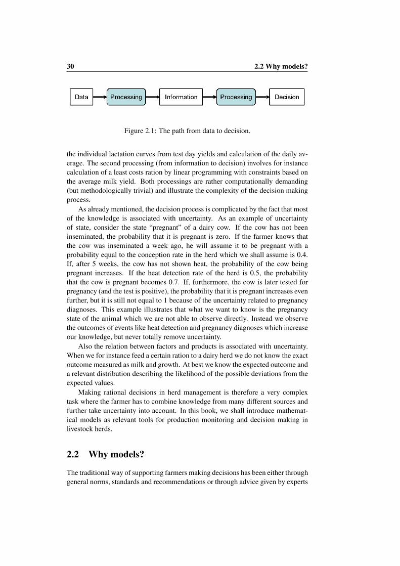
By context specific knowledge, we refer to knowledge that relates directly tothe decision problem in question. This includes information about the current stateof the unit and the effect of the state on the numerical part of the production func-tion. The source of the context specific knowledge is observations done in pro-duction. In other words, there is a direct path from data observed in production todecisions on the basis of data. This path of information may be illustrated as inFigure 2.1. In the figure, we distinguish between data and information. The term“data” is used for the raw registrations whereas “information” is data which hasbeen processed (and most often heavily reduced) to a form that can be used as abasis for decision making.
As an illustration of the path shown in Figure 2.1 we can consider the feedingdecision in dairy cows. The data could be individual test day measurements ofmilk yield, the information could be average daily milk yield during the first 24weeks of lactation, and the decision is the composition of the feed ration. In thisexample, the first processing (from data to information) involves interpolation of
30 2.2 Why models?
Figure 2.1: The path from data to decision.
the individual lactation curves from test day yields and calculation of the daily av-erage. The second processing (from information to decision) involves for instancecalculation of a least costs ration by linear programming with constraints based onthe average milk yield. Both processings are rather computationally demanding(but methodologically trivial) and illustrate the complexity of the decision makingprocess.
As already mentioned, the decision process is complicated by the fact that mostof the knowledge is associated with uncertainty. As an example of uncertaintyof state, consider the state “pregnant” of a dairy cow. If the cow has not beeninseminated, the probability that it is pregnant is zero. If the farmer knows thatthe cow was inseminated a week ago, he will assume it to be pregnant with aprobability equal to the conception rate in the herd which we shall assume is 0.4.If, after 5 weeks, the cow has not shown heat, the probability of the cow beingpregnant increases. If the heat detection rate of the herd is 0.5, the probabilitythat the cow is pregnant becomes 0.7. If, furthermore, the cow is later tested forpregnancy (and the test is positive), the probability that it is pregnant increases evenfurther, but it is still not equal to 1 because of the uncertainty related to pregnancydiagnoses. This example illustrates that what we want to know is the pregnancystate of the animal which we are not able to observe directly. Instead we observethe outcomes of events like heat detection and pregnancy diagnoses which increaseour knowledge, but never totally remove uncertainty.
Also the relation between factors and products is associated with uncertainty.When we for instance feed a certain ration to a dairy herd we do not know the exactoutcome measured as milk and growth. At best we know the expected outcome anda relevant distribution describing the likelihood of the possible deviations from theexpected values.
Making rational decisions in herd management is therefore a very complextask where the farmer has to combine knowledge from many different sources andfurther take uncertainty into account. In this book, we shall introduce mathemat-ical models as relevant tools for production monitoring and decision making inlivestock herds.
2.2 Why models?
The traditional way of supporting farmers making decisions has been either throughgeneral norms, standards and recommendations or through advice given by experts

2.2 Why models? 31
(agricultural consultants or veterinarians). The first method completely ignores thefact that production systems, farmers’ preferences and constraints vary from caseto case. Thus decisions based on general standards are typically non-optimal in theindividual case. The strength of the expert is the ability to include knowledge onthose individual conditions in the decision making process. The weakness of theexpert on the other hand is the very limited capacity of humans to combine infor-mation from different sources in a consistent way. Furthermore, the ability of anexpert to deal with uncertain information is usually not good.
The appearance of personal computers in the eighties soon lead to great expec-tations for using computers as a tool for decision support in agricultural production.The idea was to bring the knowledge of the experts directly to the dairy farmers bymeans of the so-called rule-based expert systems. McKinion and Lemmon (1985)concluded that expert systems “... are the ideal conduit of new knowledge fromthe agricultural scientists’ laboratory to usage at the farm level ...” and “... oncedeveloped they can raise the performance of the average worker to the level of anexpert”. In other words, an expert system tries to mimic a human expert (and ul-timately replace him). The philosophy behind is an almost blind belief in expertknowledge. As a management scientist realizing the complexity of decision mak-ing such a belief is very hard to share. Under all circumstances it may be concludedthat an expert system will never be better than the experts it mimics.
A promising way to circumvent the shortcomings of general standards and ex-pert advice is to construct a model representing the production unit and the decisionproblem. The main advantages of model based decision support include in the idealsituation the ability to take individual conditions into account, a concise frameworkfor combination of information from different sources, direct representation of un-certainty and efficient search algorithms for determination of optimal decisions.Most models may be described by their structure representing general knowledgeand their numerical contents representing context specific information.
Models may further contribute with extensive sensitivity analyses concerningoptimal decisions, deviating conditions and parameter values. It is therefore be-lieved by many herd management scientists that models may provide better deci-sions than experts, and that is indeed the reason for constructing and using them.Disadvantages mostly refer to the model building process which may be a verydemanding task and to the operational use of the models which (because of thecomplexity of real world problems) may require computer calculations of vast di-mensions.
In order to be used for decision support a model must represent all kinds ofknowledge needed for making the decision in question. Furthermore, the precisionof the knowledge (“level of uncertainty”) has to be represented for a correct eval-uation of alternative decisions. How to represent knowledge is the first importantissue in model construction. A second and a third important issue are how to obtainthe desired knowledge and what algorithms to use in search of optimal decisions.

32 2.3 Knowledge representation
2.3 Knowledge representation
Models are in general used for representation of all kinds of knowledge mentionedin Definition 2. They furthermore cover the processing of data into informationand the processing of information into decisions as illustrated in Figure 2.1. In thefollowing subsections we illustrate some principles of knowledge representation(including representation of the uncertainty).
2.3.1 The current state of the unit
Let us assume that the relevant unit is a dairy cow and we have to make a decisionconcerning for instance culling, insemination or medical treatment. Such decisionsare all based on the expected future performance of the animal which in turn de-pends on the observed performance until now. The distinction between observedand future performance is important. Historical records are only relevant as a basisfor prediction, since it is a well known fact that it is not possible to change the past.In other words, when we choose the traits to be represented in a model we want thebest possible basis for prediction. Most often the state of an animal is modeled as aset of variables each representing a relevant trait like parity, stage of lactation, ob-served milk yield, days open, mastitis history etc. We shall refer to such variablesas “state variables” included in the “state space”.
It is important to realize that the best variables to be used for prediction offuture performance are often neither observed nor observable. As an example,consider the trait “milk yield”. The reason for including a measure of milk yieldas a state variable is to be able to predict future milk yield. What we observe inpractise is test day milk yield, but a more relevant variable to use for predictionwould be some kind of abstract “milk yield capacity” of the cow in question. Thisis common knowledge to any dairy farmer who uses estimates like 305 days milkyield for evaluation of his cows, because individual test day milk yields are sub-ject to large random fluctuations and, furthermore, depend very much on stage oflactation.
We therefore conclude that a variable measuring the milk yield capacity of thecow is relevant. An other obvious state variable is the pregnancy state of the cow.Neither of these variables are observable, but they are essential in the prediction ofthe future performance. In Figure 1 the relation between these unobservable statevariables and a number of directly observable variables is illustrated. An ellipse inthe figure is a random variable, and an arrow indicates a causal relation betweentwo variables. Variables labeled by an asterisk are observable. Others are not.
The abstract milk yield capacity is the combined effect of genotype and perma-nent environment. Since the observed test day milk yields depend on the capacitythere are arrows from the capacity to individual monthly test day records. But theover-all capacity is not the only effect influencing test day milk yield. Also tem-porary environmental factors (“Temp 1”, . . . , “Temp 6” in the figure) influence themilk yield on a specific day. It is reasonable to assume that short term environmen-

2.3 Knowledge representation 33
Figure 2.2: A conceptual model describing the milk yield, pregnancy and heat stateof a dairy cow. Only variables marked by an asterisk are directly ob-servable.
tal effects are auto-correlated which is illustrated by arrows from each effect to thefollowing. In short term predictions, an estimate of the temporary environmentaleffect combined with an estimate of the over-all capacity is necessary. In long termpredictions the capacity may be sufficient.
As concerns the pregnancy state of the cow we logically observe that preg-nancy may influence test day milk yield (at least in the late part of lactation), butof course not the over-all capacity. Also for this variable we should notice thatit is unobservable. We may look for heat and perform pregnancy diagnosis, butneither method is exact. It is very important in prediction, that the uncertainty isrepresented. Otherwise there is an obvious risk of biassed estimates.
Until now we have only described the relations in general terms, but the net-work shown in Figure 2.2 may also be implemented numerically, so that each timea new test day milk yield is recorded, the capacity and the temporary effect are re-estimated. The tool for this kind of knowledge representation is Bayesian Networksas described by Jensen (2001). Bayesian Networks represent a very promising toolfor knowledge representation and knowledge management in animal productionmodels. Various software tools are available for construction and implementationof Bayesian Networks. There are already several examples of applications to dairycattle. Dittmer (1997) uses the technique for prediction of calving dates; Hogeveenet al. (1994) as well as Vaarst et al. (1996) used Bayesian Networks for mastitis di-agnosis; Rasmussen (1995) constructed a system for verification of parentage forJersey cattle through blood type identification, and McKendrick et al. (2000a) usedthe method for diagnosis of tropical bovine diseases.
Although Bayesian networks are obvious to use in this context we should real-ize that other methods are also available. In particular Kalman filtering techniqueshave been used for estimation of unobservable variables. The whole setup shown

34 2.3 Knowledge representation
in Figure 2.2 (except for the pregnancy related variables) has been formulated byGoodall and Sprevak (1985). In their model, the over-all capacity was representedby the 3 parameters of the Wood lactation curve. Each time the test day milk yieldwas recorded the parameters and the temporary effect were re-estimated provid-ing a good basis for prediction of future milk yield. Other examples of similartechniques are Thysen (1993a) who monitored and predicted bulk tank somaticcell counts; Thysen and Enevoldsen (1994) who monitored heat detection ratesand pregnancy rates at herd level, and de Mol et al. (1999) who used the Kalmanfiler for analysis of sensor-based milk parlour data. Finally, Madsen et al. (2005) aswell as Madsen and Kristensen (2005) used the method for monitoring the drinkingpattern of growing pigs.
The strength of these Bayesian methods (Kalman filtering and Bayesian net-works) is that uncertainty about the true level of important variables is directly rep-resented. Furthermore, the methods provide a concise framework for combinationof knowledge from different sources thus increasing the precision of knowledge asfurther observations are done.
2.3.2 The production function
As discussed in Chapter 1, the relation between factors and products is in usuallyrepresented by a production function taking the factor levels as arguments andreturning the resulting production. As an example, we shall consider the relationbetween feeding and milk production in dairy herds. Assume that the cows arefed a ration consisting of n feedstuffs in the amounts x1, x2, . . . , xn. In principle,the production function should take x1, x2, . . . , xn as arguments, but our generalknowledge tells us that it is more relevant to consider the amounts of energy, z1,protein, z2, and fat, z3. If the nutritional contents of the individual feedstuffs areknown, we may easily calculate z1, z2 and z3 from x1, x2, . . . , xn. If, for instance,the energy concentration of feedstuff i is ρ1i, the total energy content z1 becomes
z1 =n∑
i=1
ρ1ixi. (2.1)
A quadratic production function taking the energy, protein and fat contents ofthe feed ration as arguments was estimated already by Thysen (1983). If y is themilk yield, the relation is y = f(z1, z2, z3), where the production function f maybe written as
f(z1, z2, z3) = c1z1 + c11z21
+ c2z2 + c22z22
+ c3z3 + c33z23
+ c12z1z2 + c13z1z3 + c23z2z3.
(2.2)
where the cs are constants. Since Eq. (2.2) is a deterministic function we concludethat the value returned for the milk yield y is only the expected value. In practise,

2.3 Knowledge representation 35
the actually observed milk yield may vary considerably for the same feed ration.The first step in order to represent this uncertainty is to include a random term e inthe equation, so that the random milk yield Y becomes
Y = f(z1, z2, z3) + e (2.3)
where E(Y ) = y. Usually a normal distribution may be assumed for the randomterm e. This representation is a considerable improvement. If the uncertainty isignored, the influence of feeding on milk yield will be over-estimated and wrongdecisions may be made. However, even Eq. (2.3) ignores a significant part of theuncertainty. It assumes implicitly that the true contents of energy, protein and fatare known. In practise that is not the case. Cows are fed a mixture of some kind ofroughage (for example silage) and concentrates. In particular the nutritional con-tents of the roughage is uncertain. The values used as a basis for ration formulationmay either be standard values from tables or they may origin from some kind ofanalysis of a sample of the roughage.
If we simplify the problem to feeding a mixture of silage, x1, and concentrate,x2, and only consider energy, the uncertainties may be illustrated as in Figure 2.3.Just like in Figure 2.2, each ellipse represents a state variable. Again, those markedby an asterisk are observable, others are not. The variable “Milk yield*” is at herdlevel and therefore directly observable. The variables “Silage true”, “Concentr.*”,“Silage obs.*” and “Ration” all refer to the energy content. In particular, “Silagetrue” and “Concentr.*” are the variables ρ11 and ρ12 in Eq. (2.1).
Since we do not know the true energy content of the silage, we neither know thetrue energy content of the full ration (the uncertainty concerning the concentrateis ignored). We have to rely on the observed energy content of the silage. Theprecision of the observed value will depend very much on the method used forobservation. If we just use standard values for silage the precision will be low. Ifwe include information on the dry matter content the precision will increase and alaboratory analysis will give even higher precision. The problem is similar to thepregnancy diagnosis problem shown in Figure 2.2: - Several methods are availableeach providing its own level of precision.
Just as Figure 2.2 may be implemented numerically using Bayesian networks,the same applies to Figure 2.3. In particular it should be noticed that the arrowfrom “Ration” to “Milk yield*” numerically represents the production function fand the random term e as specified in Eqs. (2.2) and (2.3). The “Herd size*”variable is just a scaling factor.
2.3.3 Other kinds of knowledge
As concerns the attribute functions and the utility function of the farmer, modelsalso play an important role. Reference is made to Chapter 3 for a detailed discus-sion.

36 2.3 Knowledge representation
Figure 2.3: Relevant state variables describing the energy content and the result-ing milk yield of a ration fed to dairy cows. Observable variables aremarked by an asterisk.
For other kinds of knowledge (distribution of future states, constraints) therepresentation depends heavily on the modeling technique and reference is madeto later chapters.
2.3.4 Knowledge acquisition as a decision
In this section we shall focus on acquisition of the context specific knowledgerelated to the state of the unit considered. General knowledge about relevant feed-stuffs, medical treatments etc. is not discussed. Knowledge about states is obtainedthrough observations of the relevant unit. It is important to realize that to observethe unit is actually a decision. The purpose of observation is to improve knowl-edge, but on the other hand, observations are always associated with costs (eitherin money or time). In other words, making observations may be regarded as aproduction factor like animals and feedstuffs. Just like we want to determine anoptimal feeding level we must try to determine an optimal observation level. Hav-ing identified what trait of the unit is of interest (for example “pregnancy state” or“energy content”), the decisions involved include at least
• what exactly to observe?
• how to observe?
• how often to observe?
These 3 questions may together be referred to as the method, which has al-ready been briefly discussed in relation to the feedstuffs example of Figure 2.3.Since different methods have different precision and represent different costs, thechoice of method is certainly not irrelevant. When making this kind of decision,the economic value of information is important, but unfortunately, very little at-tention has been paid to that matter in herd management research. An exceptionis a very interesting research conducted by Jørgensen (1985). His results showedremarkable diminishing returns to scale for increasing number of traits observed.

Chapter 3
Objectives of production:Farmer’s preferences
3.1 Attributes of the utility function
A general characteristic of an attribute is that it directly influences the farmer’ssubjectively defined welfare and, therefore, is an element of the very purpose ofproduction. This may be illustrated by a few examples. The average milk yieldof the cows of a dairy herd is not an attribute of a utility function, because sucha figure has no direct influence on the farmer’s welfare. If, however, he is able tosell the milk under profitable conditions he will experience a monetary gain, whichcertainly may increase his welfare and, therefore, may be an attribute. In otherwords, the purpose of production from the farmer’s point of view could never be toproduce a certain amount of milk, but it could very well be to attain a certain levelof monetary gain.
Animal welfare may in some cases be an attribute of the utility function. Whetheror not it is in the individual case depends on the farmer’s reasons for consideringthis aspect. An argument could be that animals at a high level of welfare probablyalso produce at a higher level and thereby increase the monetary gain. In that case,animal welfare is just considered as a shortcut to higher income, but it is not con-sidered to be a quality by itself. Accordingly, it should not be considered to be anattribute. If, on the other hand, the farmer wants to increase animal welfare evenif it, to some extent, decreases the levels of other attributes like monetary gain orleisure time then it is certainly relevant to consider it to be an attribute of the utilityfunction.
This discussion also illustrates that attributes are individual. It is not possibleto define a set of attributes that apply to all livestock farmers. In the followingsection, however, we shall take a look at some examples of typical attributes offarmers’ utility functions.

38 3.2 Common attributes of farmers’ utility functions
3.2 Common attributes of farmers’ utility functions
Typical attributes describing the welfare of a livestock farmer include:
• Monetary gain
• Leisure time
• Animal welfare
• Working conditions
• Environmental preservation
• Personal prestige
• Product quality
In this section, we shall discuss each of these attributes and focus on how todefine relevant attribute functions in each case and how to compare contributionsfrom different stages.
3.2.1 Monetary gain
It seems very unlikely that monetary gain should not be an attribute of all profes-sional farmers’ utility function. In many practical cases it is even the only oneconsidered when decisions are made. Usually, it is very easy to define the attributefunction of monetary gain. If we assume product prices py1 , . . . , pyn and factorprices px1 , . . . , pxm to be fixed and known, the partial attribute function simplybecomes (assuming that monetary gain is the 1st attribute):
u1t = h1(Yt,xt) =n∑
i=1
pyiYti −m∑
i=1
pxixti. (3.1)
Monetary gains from different stages are not directly comparable. If a certainamount of money is gained at the present stage, it is possible to invest it and earninterest, so that the amount has increased at the following stage. The usual way toaccount for that is by discounting, so that we deal with the present value of futuremonetary gains. If we assume all stages to be of equal length, and the interest rateto be constant, the present value of monetary gains from N stages is calculated as:
νN =N∑
t=1
βt−1u1t, (3.2)
where 0 < β ≤ 1 is the discount factor usually calculated as
β = e−r, (3.3)
where r is the interest rate per stage. For further information on the theory andprinciples of discounting, reference is made to textbooks on economics.

3.2 Common attributes of farmers’ utility functions 39
3.2.2 Leisure time
Just like monetary gain, leisure time is probably an attribute of all farmers’ utilityfunctions. It is, however, slightly more complicated to represent it, because notonly the total value, but also the distribution over time (day, week, year) is relevant.Since leisure time is the counterpart of work, it may therefore be relevant to split upthe factor labor into several sub-factors like for instance work on weekdays from 6am to 6 pm, x1, work on weekdays from 6 pm to 6 am, x2, work in weekends from6 am to 6 pm, x3, work in weekends from 6 pm to 6 am, x4, etc. These sub-factorsare assumed to refer to the farmer’s own work, whereas the work by employees hasto be represented by other sub-factors.
Using these sub-factors we may quite easily at any stage t calculate correspond-ing sub-attributes like total leisure time u2t1, leisure time in weekends u2t2, duringday time u2t3 etc. If the stage length in days is denoted as D, these sub-attributesare objectively calculated as for instance total leisure time in hours (where the in-dex j refers to different sub-periods):
u2t1 = 24D −∑
j
xj , (3.4)
and correspondingly for other sub-attributes. There exists no general over-all par-tial attribute function h2 for leisure time, because the properties of that functiondepends on the farmer’s individual (subjective) preferences. It seems however, rea-sonable to assume, that it may be defined in each individual case as a function of anumber, v, of objectively calculated sub-attributes like those discussed, i.e.
u2t = h2(u2t1, . . . u2tv). (3.5)
As concerns the comparison of values relating to different stages, the sub-attributes are to some extent additive (e.g. total leisure time). In other cases itmay be more relevant to look at the average value (e.g. work load in weekends)and/or the maximum value. If, for instance, x3 and x4 from the example above areboth zero, it means that the farmer does not have to work at all during the weekend,which some farmers would give a high priority. Correspondingly, if u2t1 = 24Dfor a stage, it means that the farmer is able to have a vacation.
3.2.3 Animal welfare
While monetary gain and leisure time are probably attributes of all farmers’ util-ity functions (albeit that the relative weights may differ), the situation is differentwith animal welfare. There is no doubt that some farmers will include the attribute,but since the level of animal welfare has no direct consequences for the farmer’swelfare it is probably ignored by others. It does not mean that the farmer neces-sarily ignores animal welfare, but the reason for considering it may only be forlegal reasons or because it to some extend affects the production and consequentlyother attributes like monetary gain and/or labor. If that is the case, animal welfare

40 3.2 Common attributes of farmers’ utility functions
is only considered as far as to meet legal demands and not to affect the other at-tributes. In such a situation it should not be defined as a separate attribute of theutility function.
Recalling Section 3.2.1 we note that monetary gain is an attribute which mayobjectively be represented by a single numerical value. As concerns leisure time,we needed several numerical values (or sub-attributes) for an objective representa-tion. If we want to express that attribute as a single numerical value it is unavoid-able a subjective personal value derived from the preferences of that particularfarmer. Another farmer would probably attach different weights to the various ob-jective sub-attributes involved and, therefore, his over-all evaluation of the scenariowould differ.
When it comes to an attribute like animal welfare, it is even a question whetherobjective sub-attributes exist. In general, the assessment of the very concept ofanimal welfare is a problem. The discussion of a proper definition of welfare is oldas the examples collected below by Kilgour and Dalton (1984) will illustrate:
• A wide term that embraces both the physical and mental wellbeing of theanimal (Brambell, 1965).
• Existence in reasonable harmony with the environment, both from an etho-logical and physiological point of view (Anonymous, 1977).
• Welfare can be satisfied if three questions can be answered in the affirmative:(a) Are the animals producing normally? (b) Are they healthy and free frominjury? (c) Is the animal’s behaviour normal? (Adler, 1978).
• Welfare is a relative concept. Profit is a matter related to welfare and deter-mining the relationship between welfare and profit is a scientific matter. Thechoice between welfare and profit is an ethical matter (Brantas, 1978).
• Considering that while an animal is producing protein without observablesigns of pain, then it can be considered to be comfortable. Distress, strain,gross abuse and suffering are used to describe unfavorable circumstances... the presence of raw flesh or heavy bruises would be classified this way,but callouses or hard skin caused by concrete floors and producing no painwould not be classed as distressing (Randall, 1976).
• On a general level it is a state of complete mental and physical health wherethe animal is in harmony with its environment. On an empirical level it maybe measured by studying an animal in an environment which is assumed tobe ideal, and then comparing it with an animal in the environment underinvestigation (Hughes, 1976).
• Handling animals in the least disturbing manner with full consideration fortheir normal species-specific behaviour requirements (Kilgour, 1987).

3.2 Common attributes of farmers’ utility functions 41
None of the definitions listed are appropriate in this context. A more consistentapproach seems to be to consider animal welfare analogously to human welfare asdiscussed by Sandøe and Simonsen (1992). If we accept this approach, the welfareof an animal may be described by a utility function involving a number of at-tributes each representing an element of animal welfare. The principles are exactlythe same as with the farmer’s utility function, but the attributes considered natu-rally differ. Animal welfare has nothing to do with monetary gain, environmentalpreservation or product quality. Instead, relevant attributes might be:
• Absence of hunger
• Absence of pain
• Thermal comfort
• Absence of fear
• Pleasure, joy
Just like the farmer’s utility, animal welfare may be controlled by the dynamicallocation of factors to the production processes. Obviously, absence of hunger isensured by an appropriate supply of feeds, but it is important to realize that whatmatters in relation to welfare is the subjective experience by the animal. It is cer-tainly possible to feed animals in such a way, that all requirements for maintenanceand production are satisfied, but the animal nevertheless feels hungry. Such a situ-ation may occur if an animal is fed a very concentrated ration as it is typically thecase with sows during the gestation period. Even though all physiological concernsare met, the welfare of the animal may be violated.
As concerns pain, many factors are involved: Physical injuries caused by inap-propriate housing conditions may expose the animal to pain. The same applies ofcourse to injuries caused by other animals in the flock. An other source of pain isdisease, which may be prevented or cured by drugs, vitamins, minerals or feedingin general as well as by the housing conditions.
By thermal comfort we mean that the animal neither feels cold or too warm.This may be achieved in many different ways involving many different factors.If an animal feels cold, we may for instance install a heating system, reduce theventilation, increase the number of animals per square meter, or supply the animalwith straw for bedding.
It seems reasonably to assume that farm animals are able to experience fear. Ifwe accept this assumption we have to consider how to prevent it. The two mostimportant factors in this respect are probably labor and other animals. A negativeinfluence from labor is prevented by appropriate daily routines and the influencefrom other animals is regulated through flock sizes and re-grouping.
As concerns the last attribute mentioned (pleasure, joy) it is a question whetherit makes sense in relation to animals, but according to Sandøe and Simonsen (1992)

42 3.2 Common attributes of farmers’ utility functions
several researchers define this attribute and even attributes like satisfaction andexpectation as elements of animal welfare.
Having identified the attributes is of course only half the way to an operationalrepresentation of animal welfare as a possible attribute of the farmer’s utility func-tion in relation to herd management. Since the attributes of animal welfare repre-sent the animals’ subjective experience, they cannot be measured directly. All thatcan be measured are physiological, behavioral, pathological and other objective pa-rameters which may serve as evidence for the occurrence of the relevant subjectiveexperiences. Sandøe and Simonsen (1992) therefore argue that animal welfare re-searchers have to find out which measurable parameters will serve as indicators ofthe occurrence of which experiences. This is an other example of a situation wherethe herd management scientist depends on results achieved in other research dis-ciplines. What is actually measured are typically parameters like hormone levels,conflict and abnormal behavior, results of various sorts of choice tests conductedand disease incidences. Sandøe and Simonsen (1992) refer to Dawkins (1980) andFraser and Broom (1990) for a more full and detailed account.
Reference is also made to Sandøe and Hurnik (1996) for a collection of arti-cles discussing concepts, theories and methods of measurement in relation to thewelfare of domestic animals.
An other problem is how to combine the conclusions regarding individual at-tributes into the aggregate notion of over-all animal welfare, which is the possibleattribute of the farmer’s utility function. Since, however, this problem is analogousto the problem of combining the various attributes of the farmer’s utility function,reference is made to Section 3.2.2, where that issue is discussed.
3.2.4 Working conditions
Also the working conditions may affect the farmer’s welfare. When working inbarns, dust may contaminate the respiratory system and even damage the lungs.Correspondingly, very hard work (heavy burdens etc.) may harm the back. Itis probably not possible to express the working conditions objectively by a sin-gle numerical attribute. It must, however, be assumed that if the general workingconditions are so bad that they are a threat to the farmers permanent health con-dition improvements will have a very high priority in the utility function. Whenexpressing the over-all value of the attribute over several stages it may therefore berelevant to define it as (assuming that the working conditions are the 4th attributeof the utility function):
u4N = mintu4t , (3.6)
where u4t, 1 ≤ t ≤ N , is the resulting value at stage t of the attribute representingthe working conditions. In words, Eq. (3.6) says that what matters to the farmerare the worst working conditions experienced during the N stages.

3.2 Common attributes of farmers’ utility functions 43
3.2.5 Environmental preservation
Just like some of the previously discussed attributes it may also be relevant initiallyto define a number of sub-attributes u5t1, . . . , u5tv each representing an aspect ofenvironmental preservation. In most cases they may be objectively calculated asnumerical figures even though the precision may vary. An example of such a sub-attribute is according to Jensen and Sørensen (1999) the net loss of nutrients (e.g.nitrogen) to the environment which may be calculated as
u5t1 =m∑
i=1
cxixti −n∑
i=1
cYiYti, (3.7)
where cxi and cYi are the concentrations of the nutrient in question in the ith factorand the ith product, respectively. Other relevant sub-attributes mentioned by Jensenand Sørensen (1999) include the total consumption of energy and indicators of therisk of residues of pesticides in the environment.
When dealing with the leisure time attribute we concluded that no general over-all partial attribute function exists. For an individual farmer, however, we assumedthat such a subjectively defined function exists as illustrated by Eq. (3.5). As con-cerns environmental preservation, the aggregate attribute function probably alsohas to be subjectively defined, but, in this case the reason is merely lack of knowl-edge on the relative importance of the sub-attributes in relation to environmentalpreservation.
When the attribute is evaluated over several stages, calculation of average val-ues of the sub-attributes are most often the relevant method.
3.2.6 Personal prestige
Already by using the word “personal” we suggest that we are dealing with a sub-jectively defined attribute. In many cases, personal prestige has something to dowith a high level of productivity (e.g. milk yield per dairy cow or litter size persow), the presence of a factor of a particular kind (e.g. a milking parlor or a bigtractor) implying that we are dealing with sub-attribute functions of the kind
u6t1 =Yti
xtj, (3.8)
(where Yti and xtj are, for instance, the total milk yield and the number of cows atstage t) or the kind
u6t2 =
1, xti > 00, xti = 0
. (3.9)
Even though the list of sub-attributes is highly subjective, the calculation oftheir numerical values are, as illustrated, most often objective. Otherwise theirworth as the basis of personal prestige would be lacking. Also the over-all partialattribute function h6 is subjectively defined.
44 3.3 From attributes to utility
3.2.7 Product quality
All farmers are probably interested in product quality to the extent that it influ-ences the price of the product (e.g. the hygienic status of milk). If, however, thatis the only reason for considering product quality, it should not be defined as anattribute of the farmer’s utility function. If the farmer is interested in product qual-ity also if it is independent of (or even in conflict with) monetary gain and otherattributes already included then it is relevant to consider it as an attribute of theutility function.
The relevant sub-attributes to consider will of course depend on the product,but typical examples when dealing with animal production are the hygienic status,the risk of residues of medicine or indicators of the nutritional value for humans(e.g. fat or protein percentage).
3.3 From attributes to utility
3.3.1 Aggregation of attributes, uncertainty
Having identified the attributes of a farmer’s utility function we face the problemof how to combine these single attributes into an aggregate over-all utility of thefarmer. The examples of the previous section clearly illustrate that typical attributesare very different in nature and measured in different units (e.g. monetary gain andanimal welfare). When we use the attributes in a planning situation we furthermoreface the problem that we are not able to calculate exact values relating to futurestages as discussed in relation to Eq. (1.7). We have to consider the attributes(and thereby utilities) of future stages as random variables reflecting that we areproducing under risk. In other words, the farmer has to make decisions based ondistributions of attributes and utilities rather than fixed values.
3.3.2 Single attribute situation: Risk
In the most simple case the farmer’s utility function only includes one attribute, i.e.
UN = g(uN ), (3.10)
where uN is the aggregate value of the attribute over N stages. For convenience,we shall assume that the attribute is monetary gain, but in principle it could be anyattribute. In a real situation it is hardly likely that a utility function only dependson one attribute, but the considerations below are also relevant if we consider adecision that only influences one attribute, so that the remaining attributes may beconsidered as fixed.
In order to illustrate the nature of a typical single-attribute utility function weshall initially consider a question: How do we feel about earning an extra fixedamount of money? We shall denote our present annual income as a, and the po-tential extra income as ∆a (where ∆a > 0). There is probably no doubt that we

3.3 From attributes to utility 45
Figure 3.1: A typical single attribute utility function
would all prefer the total income a+ ∆a to a no matter the actual values of a and∆a. In other words, the utility function g must have the property that
g(a+ ∆a) ≥ g(a) (3.11)
for ∆a > 0.In order to be able to answer the question more specifically, it is not sufficient
information just to know that ∆a is positive. We also have to know the valueof not only ∆a, but also of a. A simple example illustrates this. If our presentannual income is a million (i.e. a = 1, 000, 000) we are probably rather indifferentto earning an extra amount of say ten thousand (i.e. ∆a = 10, 000). If, on theother hand, our present annual income is only fifty thousand (a = 50, 000), wewould regard the same option as a considerable improvement of our situation. Inother words, the marginal utility of the same monetary gain depends heavily on thepresent level of income. This is illustrated in Figure 3.1 which shows the typicalcourse of a single attribute utility function defined as
U = uα, (3.12)
where, most often, 0 < α < 1. In Figure 3.1, α = 13 . For a discussion of
other common algebraic representations of utility functions, reference is made toAnderson et al. (1977).

46 3.3 From attributes to utility
Now, assume that we have to choose between two alternative actions. Since ac-tions always relate to the allotment of factors, we shall denote them as x1 and x2,respectively. The resulting production from these actions are correspondingly de-noted as Y1 and Y2. Applying Eqs. (1.1) and (3.1) we may calculate the monetarygain under action 1 as:
u11 =
n∑i=1
pyi
(fi(x1) + e1i
)−
m∑i=1
pxix1i =
n∑i=1
pyifi(x1)−m∑
i=1
pxix1i +ε1, (3.13)
where the random variable ε1 is defined as
ε1 =n∑
i=1
pyie1i . (3.14)
The monetary gain under action 2 is calculated correspondingly. Assumingfixed prices, the only random elements of the monetary gains are ε1 and ε2. Withoutloss of generality, we may assume that E(ε1) = E(ε2) = 0. Eq. (3.13) maytherefore be written as
u11 = E(u1
1) + ε1. (3.15)
Let us assume that E(u11) = 100 and E(u2
1) = 105. If the outcome is knownwith certainty (i.e. P(ε1 = 0) = P(ε2 = 0) = 0), the choice between the twoactions is easy. Using the utility function defined in Eq. (3.12) we may calculatethe corresponding utilities as U1 = 1001/3 = 4.64 and U2 = 1051/3 = 4.72implying that action 2 is preferred over action 1. This is certainly not surprising,and in fact we only needed the logically deduced Eq. (3.11) in order to arrive atthe same conclusion.
If, however, risk is involved the situation is more complicated. By risk we meanthat the random variables ε1 and ε2 have known distributions with variances greaterthan zero. A simple numerical example shall illustrate how this may influence theexpected utility associated with each of the two alternative actions. In Table 3.1,the assumed distributions of ε1 and ε2 are specified, and the resulting expectedutilities are calculated. It should be emphasized that the expected monetary gainsunder the two actions are still 100 and 105, respectively.
It may surprise to observe that even though the expected monetary gain underaction 2 is higher than under action 1, the opposite applies to the expected utilities.Thus in the example we should indeed prefer action 1 over action 2. The explana-tion is simply that action 2 is more risky than action 1, and since the applied utilityfunction only modestly rewards outcomes greater than the expected value but heav-ily punishes lower outcomes (cf. Figure 3.1), the expected utility of a risky actionwill always be lower than the expected utility of a less risky action having the sameexpected outcome.

3.3 From attributes to utility 47
Table 3.1: Probability distributions and expected utilities of two alternative actions.Action 1 Action 2
ε1 u11 P(ε1) U1 ε2 u2
1 P(ε2) U2
-10 90 0.25 4.48 -65 40 0.25 3.420 100 0.50 4.64 0 105 0.50 4.7210 110 0.25 4.79 65 170 0.25 5.54Expected utility, E(U1) 4.64 Expected utility, E(U2) 4.60
The fact that maximization of expected utility is the relevant criterion for choos-ing between risky actions follows from the so-called expected utility theorem whichis discussed by Anderson et al. (1977, p 65-69). The theorem may be deducedfrom only three perfectly reasonable axioms describing consistent human attitudesto risky choices. The same axioms also ensure the very existence of a unique sub-jective utility function.
A common numerical representation of the risk associated with an action is thevariance of the outcomes. In the example we may directly calculate the variancesfrom Table 1. Under action 1 the variance is V 1 = 0.25× (−10)2 + 0.50× 02 +0.25 × 102 = 50. The corresponding variance under action 2 is V 2 = 0.25 ×(−65)2 + 0.50× 02 + 0.25× 652 = 2112.5 indicating a far more risky action.
In the single attribute situation, it is only because of random variation (i.e.risk) that we have to consider the concept of utility and the shape of the functionconverting outcomes to utilities. In many cases it may therefore be more naturalto use the expected monetary gain and the variance directly in the evaluation ofrisky actions. That approach is called (E,V) analysis. The idea is to draw so-callediso-utility curves in a diagram where the x axis is the variance and the y axis isthe expected monetary gain. An iso-utility curve has the property, that all locialong the curve represent mean-variance combinations that yield the same level ofutility. Any risky action with known expected gain and variance may be plottedas a locus in the diagram. By comparing the loci of the actions with the course ofthe iso-utility curves, the action representing the highest expected utility may bechosen.
In Figure 3.2, iso-utility curves representing 3 constant levels of utility areshown in an (E,V) diagram. If we plot the two actions from the numerical exampleof Table 3.1 in the diagram (recalling that Action 1 had the lowest variance and thelowest expected monetary gain) we easily see that action 1 represents the highestexpected utility.
In the discussion of this section, we have implicitly assumed that the farmerin general regards risk as something that should be minimized. In other words weassume him to be risk averter. The concave utility curve of Figure 3.1 representsa risk averter. At least in theory, a farmer may be risk preferrer. In that case hisutility function is convex. Also in that case, Eq. (3.12) may be used as an algebraicrepresentation of the utility function. For a risk preferrer, however, the parameter

48 3.3 From attributes to utility
Figure 3.2: Iso-utility curves for 3 levels of utility. The two actions defined in Table3.1 have been plotted in the diagram.
α has to be greater than 1. For a discussion of those aspects, reference is made toAnderson et al. (1977), whom we also refer to for a discussion of how to identify afarmer’s utility function in practise.
3.3.3 Multiple attribute situation
In case that an action influences more than one attribute of the farmer’s utilityfunction we have to consider not only how each action affects each attribute, butalso how much weight relatively the fulfilment of each attribute should be given.Animal breeding scientists face a completely analogous problem when they definebreeding goals involving several traits as illustrated by a small example. Let usassume that the three traits milk yield, daily gain and fertility are relevant whendairy sires are selected for breeding. The relative breeding values for each traitmay be estimated by usual methods, and we shall assume that we have to selectone sire among the three candidates listed in Table 3.2.
Initially, we shall only consider the first four columns of Table 3.2. If we onlyhad to choose between Sire 1 and Sire 2 there would be no problem since Sire 1 issuperior in all three traits, but when we have to choose between Sire 1 and Sire 3we face a problem, because Sire 3 is superior with respect to milk yield but inferiorwith respect to daily gain and fertility. There is no general solution to this problem,because the final choice will depend on the weight attached to milk yield relativeto the weights attached to daily gain and fertility.

3.3 From attributes to utility 49
Table 3.2: Three sires and their relative breeding values for the traits milk yield,daily gain and fertility. Index 1 and Index 2 have been calculated usingdifferent economic weights.
Sire number Milk yield Daily gain Fertility Index 1 Index 21 110 107 104 107.75 107.002 109 106 103 106.75 106.003 114 103 102 108.25 105.50
The animal breeding scientist solves the problem by defining a so-called breed-ing index which is a linear combination of the individually estimated breeding val-ues, i.e.
Bi =J∑
j=1
cjbij (3.16)
where Bi is the breeding index of the ith animal, cj is the weight attached to thejth trait, and bij is the estimated breeding value of the ith animal concerning thejth trait. If, for instance, we define the relative weight attached to milk yield to be50% and the relative weights attached to daily gain and fertility to be 25% each(i.e. c1 = 0.50 and c2 = c3 = 0.25) the breeding indexes of the three sires of theexample become as shown under Index 1 in Table 3.2. As it appears from the table,Sire 3 should be chosen. If on the other hand, the relative weight attached to dailygain was 50% leaving 25% for each of the two remaining traits (i.e. c1 = c3 = 0.25and c2 = 0.50) the breeding indexes become as shown under Index 2 leaving Sire1 as the superior one. This clearly illustrates that the relative importance attachedto the traits determines the mutual ranking of the animals.
In herd management science we do not choose among Sires but among al-ternative actions representing different factor allotments. Neither do we evaluatealternatives on breeding values but on attributes of the farmer’s utility function.Nevertheless, if in the example we replace Sire by Action, trait by attribute (milkyield by monetary gain, daily gain by leisure time, fertility by animal welfare)and index by utility, the example will still make sense. Also in herd managementit is very likely that if we, for instance, rank actions on monetary gain the rank-ing changes if we use leisure time as our criterion of evaluation instead. Also themulti-attribute utility function may be defined analogously with Eq. (3.16). Us-ing the notation of the previous sections, the utility function would just be a linearcombination of the individual attribute functions:
U =J∑
j=1
cjuj =J∑
j=1
cjhj(Y,X), (3.17)
where c1, . . . , cJ are constant values which we may assume sum to 1 without lossof generality.

50 3.3 From attributes to utility
In the animal breeding example, Eq. (3.16) says that a higher breeding valueconcerning one trait may compensate for a lower value concerning other traits.The same is expressed for attributes like monetary gain, leisure time and animalwelfare in Eq. (3.17). This is certainly a realistic property of a utility function,but, nevertheless, if the utility function is defined as in Eq. (3.17) we implicitlymake some assumptions which by a closer look may seem unrealistic. In orderto illustrate this we shall assume that only two attributes (monetary gain u1 andleisure time u2) are relevant for the management problem considered. Eq. (3.17)thus reduces to
U = cu1 + (1− c)u2. (3.18)
If we set U equal to some constant U ′, Eq. (3.18) may be rearranged into
u2 =U ′
1− c− c
1− cu1 (3.19)
implying that all combinations of u1 and u2 yielding the same utility U ′ forma linear relationship in a diagram. In Figure 3.3, three such iso-utility curves repre-senting a low, medium and high fixed level of utility U ′ are shown. The course ofthe curves illustrate that decreased leisure time may be compensated by increasedmonetary gain, and the linear relationship implies that the marginal rate of substitu-tion between the two attributes is constant. In other words, a constant improvement∆u1 of the monetary gain may compensate a constant reduction ∆u2 of leisuretime no matter whether the initial level of monetary gain or leisure time is high orlow. From Eq. (3.19) we see that the constant marginal rate of substitution is:
∆u2
∆u1=
c
1− c. (3.20)
In Figure 3.4, iso-utility curves illustrating varying marginal rates of substitu-tion between attributes are shown. Again, three fixed levels of utility are repre-sented in the diagram. As shown in the figure, the marginal rate of substitution∆u21/∆u1 is very high if we are dealing with a poor farmer with plenty of leisuretime whereas it is very low (∆u22/∆u1) in the opposite situation (a rich farmerworking all the time).
A possible algebraic representation of a utility function having iso-utility curveslike those of Figure 3.4 is:
U = uα1u
β2 , (3.21)
where (for the risk averter) 0 < α < 1 and 0 < β < 1. It should be noticed, thatif one of the attributes is left constant, Eq. (3.21) reduces to the single-attributeutility function of Eq. (3.12). For a discussion of other possible representations ofa multi-attribute utility function, reference is made to Anderson et al. (1977).

3.3 From attributes to utility 51
Figure 3.3: Iso-utility curves representing a low, medium and high fixed level ofutility calculated according to Eq. (3.18). The marginal substitutionrate ∆u2/∆u1 is constant.
Figure 3.4: Iso-utility curves corresponding to the utility function of Eq. (3.21).We have ∆u21/∆u1 ∆u22/∆u1.

52 3.3 From attributes to utility
3.3.4 Operational representation of a farmer’s utility function
Tell me, how shall I feed my cows this winter? the farmer asks. The herd manage-ment scientist answers him back: Let me know your utility function, and I shall tellyou how to feed your cows. From a theoretical point of view, the previous sectionshave illustrated that the herd management scientist is right. In order to choose anoptimal action among a set of alternatives, we need to know the farmer’s utilityfunction. In other words we have to know what attributes he includes and how theyare weighted in a specific situation. On the other hand, the farmer is off course notable to specify his utility function, so what do we do? Does the dialogue end here,or are we able to identify the utility function to an extent where it makes sense tomake decisions?
Even though for instance Anderson et al. (1977) to some extend describe howsingle- and multi-attribute utility functions are identified in practice, it remains stilla very difficult task and even the representation of relevant attribute functions forattributes like animal welfare and working conditions may be a problem.
On the other hand, we may argue that it is not always necessary to know every-thing about the utility function when an action is chosen. In several cases we maylogically conclude that incomplete information is sufficient to choose an action:
• In some cases, an action only influences one attribute. If risk is involved, itis sufficient to know the single attribute utility function. In case of a decisionnot involving risk, even the attribute function is sufficient.
• Many actions (typically those with short time horizon) only marginally in-fluence the attributes. It is therefore sufficient to know the local marginalrates of substitution between attributes. In Figure 3.4, this may be illustratedby plotting the current combination of monetary gain and leisure time anddraw a straight line with a slope equal to the marginal rate of substitutionthrough that locus. It is not claimed that this constant rate is universal, butfor marginal changes the approximation may suffice. This means that thesimple additive Eq. (3.17) is used as a local approximation to a theoreticallycorrect (but unknown) utility function with varying substitution rates.
• The utility function may only vary little over a rather large range of actions.It may be sufficient to choose a satisfactory action rather than an optimalone. This is particularly the case if a farmer’s single-attribute utility functionhas a course as illustrated in Figure 3.5. In that case it is important, that thevalue of the attribute in question is at least as high as some satisfactory levelu∗. Lower levels are punished by the utility function, but higher values arenot rewarded. The attribute in question in Figure 3.5 could for instance beanimal welfare. Most farmers will probably try to improve it if it is verylow, but having reached a certain level, they do not worry about it anymore.When they make decisions with long time horizon (for instance regardinghousing facilities) they make some decisions to ensure a satisfactory level,
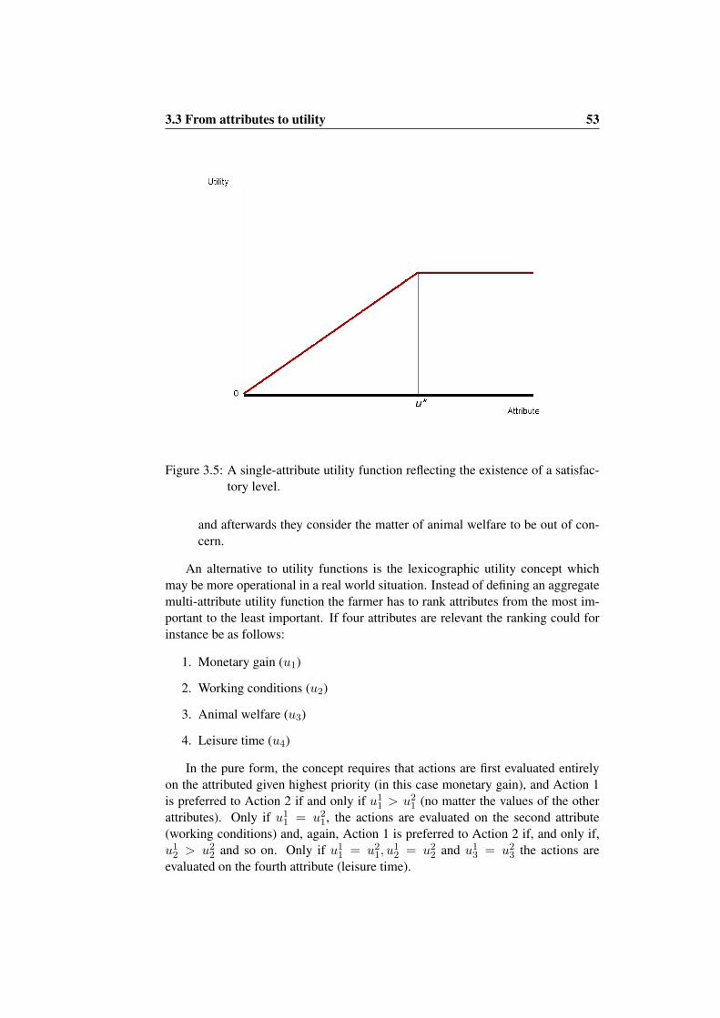
3.3 From attributes to utility 53
Figure 3.5: A single-attribute utility function reflecting the existence of a satisfac-tory level.
and afterwards they consider the matter of animal welfare to be out of con-cern.
An alternative to utility functions is the lexicographic utility concept whichmay be more operational in a real world situation. Instead of defining an aggregatemulti-attribute utility function the farmer has to rank attributes from the most im-portant to the least important. If four attributes are relevant the ranking could forinstance be as follows:
1. Monetary gain (u1)
2. Working conditions (u2)
3. Animal welfare (u3)
4. Leisure time (u4)
In the pure form, the concept requires that actions are first evaluated entirelyon the attributed given highest priority (in this case monetary gain), and Action 1is preferred to Action 2 if and only if u1
1 > u21 (no matter the values of the other
attributes). Only if u11 = u2
1, the actions are evaluated on the second attribute(working conditions) and, again, Action 1 is preferred to Action 2 if, and only if,u1
2 > u22 and so on. Only if u1
1 = u21, u
12 = u2
2 and u13 = u2
3 the actions areevaluated on the fourth attribute (leisure time).

54 3.3 From attributes to utility
The lexicographic concept may also be combined with definition of satisfac-tory levels concerning the most important attributes and then maximizing the leastimportant one subject to constraints on the others.
Finally, the obvious direct choice option should be mentioned. The farmer isjust confronted with the multi-attribute consequences of the alternative actions. Inother words, he is told that Action 1 represents a monetary gain of u1
1, workingconditions expressed as u1
2, animal welfare at the level u13 and leisure time at the
level u14. Similar values concerning the other possible actions are given, and based
on this information the farmer chooses the preferred action directly. This methodhas the obvious advantage that the advisor does not have to know the farmer’sutility function, but only the relevant attributes.

Chapter 4
Classical production theory
The neo-classical production theory is a very general theory covering almost allaspects of production optimization. It is entirely based on a symbolic representa-tion of the production function and use of general mathematical principles in thedetermination of optima. It is often said, that the neo-classical production basicallydeals with three problems:
1. What to produce.
2. How to produce.
3. How much to produce.
In this chapter we shall give a very simplified introduction to the theory byillustrating the basic marginalization principles behind the solution to the threeproblems. For detailed discussions and less restricted models, reference is made totextbooks on micro economics.
Furthermore, we shall discuss the concept of production costs by introducingkey concepts like variable costs, fixed costs, gross margin, opportunity costs, inter-nal prices and investments.
As an extension to the marginalization principles we shall introduce the con-cept of partial budgeting as an operational method to be used in regular planningof animal production.
Finally, we present a brief introduction to the classical replacement theorywhich is relevant for a wide range of decision problems in herd management.
4.1 One to one relations
4.1.1 The production function
In this section we shall use a modified version of the general production functionas presented by Eq. (1.1) in Chapter 1. We shall use the form

56 4.1 One to one relations
F (y,x) = F (y1, . . . , yn, x1, . . . xm) = 0, (4.1)
where y = (y1, . . . , yn)′ is a vector of n products, and x = (x1, . . . , xm)′ is avector of m factors. Compared to Eq. (1.1) it means that the dynamic aspect of theplanning problem is ignored by skipping the dependence on factor use in previousstages, and that the uncertainty of the outcome as illustrated by the random term ofEq. (1.1) is ignored. The purpose of this simplification is to deduct some conditionsfor optimality that are of general interest in production planning.
The interpretation of the product levels y1, . . . , yn also differs from that of Eq.(1.1) in the sense that yi now denotes the maximum achievable amount of the ithproduct given the values of y1, . . . , yi−1, yi+1, . . . yn, x1, . . . , xm. Thus, logically,products may be mutually substituted for given x (i.e. by decreasing yi, a higherlevel of yj may be reached).
It should be noticed that Eq. (4.1) reflects an assumption about immediateadaptation of production output to changes in factors.
We shall investigate a number of one-to-one relations:
What to produce: A product-product relation where we determine the optimalcombination of two products assuming fixed factor level.
How to produce: A factor-factor relation where we determine the optimal combi-nation of two factors assuming fixed production level.
How much to produce: A factor-product relation where we decide on the optimallevel of one factor used for production of one product.
4.1.2 What to produce
Assume that we only produce two products, i.e. that y = (y1, y2)′, and a fixedfactor input x = (x1, . . . , xm)′ is used in production. The production function(4.1) then reduces to
F (y1, y2,x) = 0, (4.2)
Now, let y1 vary in small steps from 0 to y+1 , where y+
1 is the maximum pro-duction possible for factor input x. For each value of y1 in the interval, we solvethe equation (4.2) with respect to y2 and plot the result in a diagram with y1 alongthe first axis and the corresponding value of y2 along the second axis. If, for in-stance, y+
1 = 10, the result could be as shown in Figure 4.1(a). We shall refer tothe curve as an iso-factor curve, because points along the curve represent productcombinations that can be achieved using the same factor input.
The curve of the figure shows possible combinations of y1 and y2 for given,fixed, factor input x. If the price of product 1 is p1, and the price of product 2 isp2, the total profit from production is simply u′ = p1y1 + p2y2 − px, where pxis the total price of the input factors. Assuming that we wish to maximize income

4.1 One to one relations 57
0
2
4
6
8
10
12
0 5 10 15 20
y 1
y2
(a) Product-product
0
2
4
6
8
10
12
0 5 10 15 20
y 1
y2
(b) Iso-income curves
0
2
4
6
8
10
12
0 5 10 15 20
y 1
y2
(c) Optimum
0
2
4
6
8
10
12
0 5 10 15 20
y 1
y 2
(d) Optimum, new prices
Figure 4.1: Optimization of product-product relation for given factor input x.

58 4.1 One to one relations
from production, we easily see that we can ignore the price of the factors (since itis fixed) and only look at the total income u (if we maximize u we also maximizeu′):
u = p1y1 + p2y2. (4.3)
Putting u = u and solving for y2, Eq. (4.3) may be rearranged to
y2 =u
p2− p1
p2y1. (4.4)
It should be noticed, that all combinations of y1 and y2 satisfying Eq. (4.4)will represent the same income level, u. Those combinations form a straight linewith slope −p1
p2in a diagram, and in Figure 4.1(b), five such iso-income lines, each
representing a fixed income level, have been added to the iso-factor curve.Since the iso-factor curve is the upper border of the achievable product com-
binations, we wish to find the combination maximizing the income. This is doneby finding the iso-income line which has the highest possible income u in the setbounded by the iso-factor curve. Figure 4.1(c) illustrates that the optimal productcombination is found on the border of the permitted area and has the property thatthe marginal substitution rate between y1 and y2 equals the slope of the iso-incomeline. In other words, the optimal combination of products is found where
dy2
dy1= −p1
p2. (4.5)
Eq. (4.5) illustrates that the optimal combination (for given production func-tion) is entirely determined by the product prices. Thus, new prices will lead to another optimal product combination as shown in Figure 4.1(d).
4.1.3 How to produce
The treatment of this problem has many similarities with the previous problem.The difference is that we now consider the optimal combination of two factors forproduction of a fixed product output. In other words, we have y = (y1, . . . , yn)′,and a variable combination of two factors x = (x1, x2)′ is used in production. Theproduction function (4.1) then reduces to
F (y, x1, x2) = 0, (4.6)
Now, let x1 vary in small steps from 0 to x+1 , where x+
1 is the consumptionof factor 1 if the production is based entirely on that factor. For each value of x1
in the interval, we solve the equation (4.6) with respect to x2 and plot the resultin a diagram with x1 along the first axis and the corresponding value of x2 alongthe second axis. If, for instance, x+
1 = 10, the result could be as shown in Figure4.2(a). We shall refer to the curve as an iso-product curve, because points along thecurve represent factor combinations that can be used to produce the same output.

4.1 One to one relations 59
0
2
4
6
8
10
0 2 4 6 8 10
x 1
x 2
(a) Factor-factor
0
2
4
6
8
10
0 2 4 6 8 10
x 1
x 2
(b) Iso-cost curves
0
2
4
6
8
10
0 2 4 6 8 10
x 1
x 2
(c) Optimum
0
2
4
6
8
10
0 2 4 6 8 10
x 1
x 2
(d) Optimum, new prices
Figure 4.2: Optimization of factor-factor relation for given output y.

60 4.1 One to one relations
The curve of the figure show possible combinations of x1 and x2 that may beused in the production of a given, fixed, product output y. If the price of factor1 is p1, and the price of factor 2 is p2, the total profit from production is simplyu′ = py− (p1x1 + p2x2), where py is the total market value of the product output.Assuming that we wish to maximize income from production, we easily see thatwe can ignore the market value of the products (since it is fixed) and only look atthe total costs c (if we minimize c we maximize u′):
c = p1x1 + p2x2. (4.7)
Putting c = c and solving for x2, Eq. (4.7) may be rearranged to
x2 =c
p2− p1
p2x1. (4.8)
It should be noticed, that all combinations of x1 and x2 satisfying Eq. (4.8)will all represent the same cost level, c. Those combinations form a straight linewith slope −p1
p2in a diagram, and in Figure 4.2(b), five such iso-cost lines, each
representing a fixed cost level, have been added to the iso-product curve.Since the iso-product curve is the lower border of the possible factor combi-
nations, we wish to find the combination minimizing the cost. This is done byfinding the iso-cost line which has the lowest possible cost c in the set bounded bythe iso-product curve. Figure 4.2(c) illustrates that the optimal factor combinationis found on the border of the permitted area and has the property that the marginalsubstitution rate between x1 and x2 equals the slope of the iso-cost line. In otherwords, the optimal combination of factors is found where
dx2
dx1= −p1
p2. (4.9)
Eq. (4.9) illustrates that the optimal combination (for given production func-tion) is entirely determined by the factor prices. Thus, new prices will lead to another optimal factor combination as shown in Figure 4.2(d).
4.1.4 How much to produce
Here we assume that one product is produced by use of only one factor. The pur-pose of the optimization is to find the optimal number of units to produce by ad-justing the input level of the factor. The production function (4.1) then reducesto
F (y, x) = 0, (4.10)
or, in a more convenient form
y = f(x), (4.11)
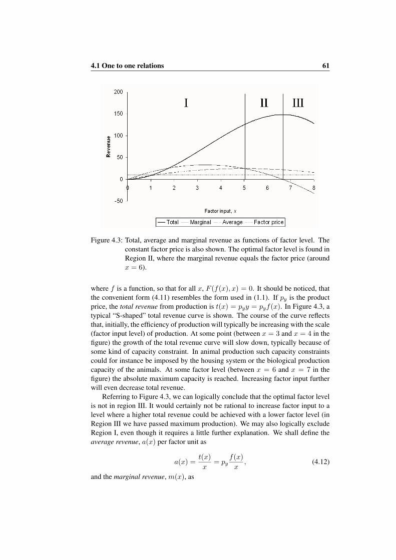
4.1 One to one relations 61
Figure 4.3: Total, average and marginal revenue as functions of factor level. Theconstant factor price is also shown. The optimal factor level is found inRegion II, where the marginal revenue equals the factor price (aroundx = 6).
where f is a function, so that for all x, F (f(x), x) = 0. It should be noticed, thatthe convenient form (4.11) resembles the form used in (1.1). If py is the productprice, the total revenue from production is t(x) = pyy = pyf(x). In Figure 4.3, atypical “S-shaped” total revenue curve is shown. The course of the curve reflectsthat, initially, the efficiency of production will typically be increasing with the scale(factor input level) of production. At some point (between x = 3 and x = 4 in thefigure) the growth of the total revenue curve will slow down, typically because ofsome kind of capacity constraint. In animal production such capacity constraintscould for instance be imposed by the housing system or the biological productioncapacity of the animals. At some factor level (between x = 6 and x = 7 in thefigure) the absolute maximum capacity is reached. Increasing factor input furtherwill even decrease total revenue.
Referring to Figure 4.3, we can logically conclude that the optimal factor levelis not in region III. It would certainly not be rational to increase factor input to alevel where a higher total revenue could be achieved with a lower factor level (inRegion III we have passed maximum production). We may also logically excludeRegion I, even though it requires a little further explanation. We shall define theaverage revenue, a(x) per factor unit as
a(x) =t(x)x
= pyf(x)x
, (4.12)
and the marginal revenue, m(x), as

62 4.2 Multi-dimensional production models
m(x) = t′(x) = pyf′(x). (4.13)
In Figure 4.3 both curves are plotted together with the total revenue, t(x). Themarginal revenue expresses how much the total revenue increases if we increasethe factor input level by 1. It is obvious that as long as adding an additional factorunit will increase total revenue by more than the average revenue so far, it will bebeneficial to do it. As it is seen in the figure, Region I is characterized by exactlythat property (that the marginal revenue is higher than the average). The optimalfactor input level must therefore be higher. Thus, optimum must be found in RegionII.
It is rather simple to show mathematically exactly where the optimum is. Wecan calculate the profit, u, from production as
u = t(x)− pxx = pyy − pxx, (4.14)
where px is the factor price. Again, we wish to maximize profit from production,so the problem reduces to finding the value of x maximizing u. According to usualmathematical theory, a maximum is determined by differentiation and solving theequation where the differentiated function is put equal to zero:
dudx = 0 ⇔
ddx(pyy − pxx) = 0 ⇔
ddx(pyf(x)− pxx) = 0 ⇔
pyf′(x)− px = 0 ⇔
m(x) = px
(4.15)
In words, Eq. (4.15) expresses that the factor input level should be increased untilthe marginal value of an additional factor unit equals the unit price of the factor. InFigure 4.3 the optimum is therefore found in Region II, exactly where the marginalrevenue is equal to the factor price.
4.2 Multi-dimensional production models
If the full multi-dimensional production function (4.1) is used, the simple marginalconsiderations of Section 4.1 will not suffice anymore. Instead, a more generalizedapproach known as Lagrange’s method based on partial differentiation and solvingof a set of linear equations must be used. We shall not discuss the method furtherhere, but refer the interested reader to a textbook of economics. For an appliedexample related to milk production under a quota, reference is made to Rasmussenand Nielsen (1985).

4.3 Limitations of the neo-classical production theory 63
4.3 Limitations of the neo-classical production theory
The neo-classic production theory provides us with a general framework for pro-duction optimization, and the marginalization criteria derived from it are applicablealso in many practical on-farm situations.
Nevertheless, the theory has several serious limitations for use in a herd man-agement context. We can summarize the limitations as follows:
Uncertainty: The neo-classical production theory assumes full certainty about theproduction outcome and the state of the factors. As discussed in details inChapter 2, uncertainty is an inherit property of the decision making processin herd management.
Dynamics: The neo-classic production model is static. It assumes implicitly thatfactors are purchased, products generated and sold within the same time in-terval. In herd management, many decisions made at an earlier stage haveconsequences for several months and years as discussed in Chapter 1.
Adaptation: It is assumed that any change in factor input results in an immediate(and full) response in output level. In a biologically based production, it isreasonable to assume some inertness in the response to changes (for instancechanges in feeding).
In order to cope with those limitations, more advanced models must be used.In the second part of this book, such models will be introduced.
4.4 Costs
It is important to distinguish between costs and payments. A payment takes placeat a certain moment (date, hours) when money is actually transferred to someoneelse. As opposed to that, costs are related to a period. The costs relating to a periodis simply the value in money of the factors used in production during the period. Itis of no relevance for the costs when the factors are actually paid for. It may verywell be in an other period, or - for that matter - never. The costs remain the same.
4.4.1 Variable costs and fixed costs: Gross margins
An important distinction is made between variable costs and fixed costs (also re-ferred to as capacity costs). By variable costs we refer to costs that vary (more orless) proportional to the scale of production. Obvious examples of variable costsare feed costs, costs of bedding material, insemination costs and medicine costs. Ifproduction is doubled, we also expect those costs to be (approximately) doubled.
By fixed costs we refer to costs that do not vary with the size of production(at least not in the short run). Examples of such costs include housing costs andsalary to permanently employed staff. No matter whether we decide to reduce
64 4.4 Costs
the production output to 50%, the costs related to farm buildings equipment andstaff remain the same. The examples also illustrate that there is no distinct borderbetween variable and fixed costs. It is, for example, obvious that costs related tostaff salary are less “fixed” than those related to the farm buildings: A herdsmanmay be fired at a certain notice, but even if we demolish the farm buildings, wewill have to continue the payments on the loan.
Because the farmer cannot really do anything to reduce the fixed costs in theshort run, the operational and tactical management will focus only on the variablecosts which are under direct control even in the short run. It is obvious that itis not sufficient just to try minimizing the variable costs (that would be easy: ifproduction is reduced to zero the variable costs will also be zero). As illustrated inFigure 4.3, the variable costs should be increased to the level where the marginalrevenue equals the marginal costs if profit is to be maximized.
In order to follow the economic efficiency of production the farmer typicallycalculates the gross margin (as defined in Definition 3) for the various productionprocesses on the farm. The processes may for instance be the production based onthe sows, the slaughter pigs and the crops.
Definition 3 The gross margin of a production process is defined for a specifiedperiod as the total revenue generated by the process during the period minus theassociated variable costs. The gross margin is also known as the contribution mar-gin.
The advantage of the gross margin concept is that it enables the farmer to com-pare over time, over processes and with other farmers. The comparison over pro-cesses is important because if the farmer finds the gross margin from slaughter pigstoo low, he might decide skipping slaughter pig production and use the facilitiesfor something more profitable (e.g. expand the sow herd).
The reason for using the gross margin (instead of net profit) for comparisonbetween farmers is that the fixed costs vary very much from farm to farm depend-ing on the housing facilities and many other circumstances. Thus, the net profit issimply not comparable over farms. The variable costs are more likely to be compa-rable. Accordingly, it makes sense to use gross margin as a measure of economicefficiency between farms.
4.4.2 Opportunity costs and internal prices
In many cases, the interpretation of the costs are straight forward: A certain amountof a factor has been used during the period. Each unit has a well-defined price,because the factor is bought at the market, and the costs are the number of unitsmultiplied by the unit price.
There are, however, many cases where more indirect considerations are needed.Examples include:
• Feeds may consist of home-grown crops.

4.4 Costs 65
• A slaughter pig production may be based on piglets from the farmer’s ownsow herd.
• The value of the animals represents a considerable amount of money.
It is obvious that the costs related to the items above should be included in thegross margin, and that is exactly where the concept of opportunity costs, as definedbelow, is relevant.
Definition 4 The opportunity cost of a factor used in production is the value of thefactor if it was used in the best possible alternative way. The name of the conceptrefers to the fact that this opportunity is lost.
When the farmer for instance calculates the gross margin for slaughter pig pro-duction, he should include the costs of the piglets no matter whether he buys themat the market, or he “buys” them from his own sow production. This is an exampleof the opportunity cost concept. By using the piglets in his own slaughter pig pro-duction, the farmer looses the opportunity of selling the piglets at the market. Theinternal price of the piglets to be used when calculating the gross margin of theslaughter pigs is simply the value of the piglets on the market. This illustrates thatif we are dealing with a factor commonly exchanged over a market, the internalprice is simply the market value.
In other cases the calculation of internal prices is more complicated, and whenthe internal price is used in planning, the value may even depend on the time hori-zon as the following example will illustrate.
Example 1 Internal production price of roughage.Dairy cows are typically fed a ration consisting of some kind of mix of roughageand concentrates. The roughage can either be based on home-grown crops, or it can(at least to some extend) be based on industrial by-products bought at the market.The decision about the ingredients of the feed ration is based on the nutritionalcontents and the price.
The price of industrial by-products is well-defined and easy to get from mar-ket information, but what about the internal price of home-grown roughage? Theanswer depends on the time horizon.
Before the growth season: At this stage the dairy farmer still has the option notto grow the roughage and instead base his feeding on industrial by-products.Such a decision will allow him to use the land intended for the roughagefor other crops to be sold at the market. If he chooses to grow roughage helooses that opportunity. The correct internal price must reflect that fact, andaccordingly, it is defined as follows:
+ Direct variable costs of roughage d+ Gross margin of alternative crop to be sold g
= Internal production price of roughage p

66 4.4 Costs
The direct variable costs include seeds, fertilizer, chemicals, and costs offuel, cultivation and machinery. The gross margin of the alternative cropincludes the market value of the crop less the variable costs associated withproduction (according to the standard definition of the gross margin conceptas given in Definition 3). For a numerical example, reference is made toExercise 4.7.2.
The internal production price defined in this way is directly comparable withthe price of feedstuffs available at the market. When planning next year’swinter feeding, it is therefore the internal production price that should beused for home grown roughage.
During the growth season: When the roughage is already growing in the fields,the option of growing an alternative crop to be sold at the market is no longeravailable. Any consideration of future feeding should therefore be based ona price setting reflecting the absence of that opportunity. Accordingly, theinternal price will be lower, because the lost gross margin of an alternativecrop should now be ignored (the option is no longer available, and you can’tchange the past).
The internal price of the roughage in this situation therefore only consistsof the variable costs from now. Variable costs until now (e.g. seeds andfertilizer) should be ignored, because they are already facts that can’t bechanged no matter what the farmer does. The internal price of a roughagealready growing in the fields is therefore typically very low. The low pricereflects the fact that when the decision to grow the roughage has already beenmade, it is in most cases unrealistic to replace it with feedstuffs bought at themarket.
It must be emphasized that these considerations assume that there is no mar-ket for the roughage. If, on the other hand, there is a market, the price usedin planning should be the market value of the roughage.
After harvest: When the roughage has been harvested, all previous costs are ofno relevance for the internal price. Those costs have already been paid, andno matter what we do, the money is spent, and it cannot be regained.
If there is a market for the roughage, the price used in feed planning shouldreflect the market value. In many cases, however, there is not really a marketfor roughage, and accordingly it is realistic to define the internal price tobe zero, simply because the roughage has no alternative value. When itis already available in the rick or the silo, it is unrealistic not to use it forfeeding.
The only relevant question is which category of animals to feed it to (theheifers, the high yielding dairy cows, the dry cows, etc.) The answer to thatquestion should be based on where the marginal contribution to the grossmargin is highest.

4.4 Costs 67
4.4.3 Investments
The unit costs of factors used entirely during one time stage are rather easy tounderstand. We use a certain amount of a feedstuff during the stage, and the unitprice is known either from the market or from calculation of internal prices.
When it comes to factors like farm buildings or inventory the cost associatedwith a given stage (e.g. a year) is more difficult to assess, simply because we usethe building or inventory for several years. We typically know the total price ofe.g. a building when it was built or purchased, but that value may be very high,and it would not be “fair” to charge the full amount to the year of construction.Intuitively, it seems reasonable to disperse the cost over several years.
When dispersing the investment, the key question is for how long we can usethe asset in production. If it is a farm building it may for instance be 20 years, andless for inventory. Let I be the initial investment (the price of the asset at purchase)and n be the number of years that we expect to use the asset. It would be temptingjust to calculate the annual costs, c, as c = I/n, but from an opportunity cost pointof view this is not correct. Usually, I represents much money, and by using it forinvestment in an asset means that the farmer looses the opportunity of investing themoney in an alternative way (he might for instance buy stocks or bonds).
The lost returns (typically in the form of interests) from the alternative invest-ment should also be included in the annual costs of the investment. In economics,there are standard methods for calculation of annual costs of investments. If I, cand n are defined like before, and furthermore r is the interest rate of the alternativeinvestment, the annual costs are calculated as
c = Ir
1− (1 + r)−n. (4.16)
It should be noticed that the annual costs calculated this way includes the de-preciation (loss in value) as well as the interest costs.
Example 2 Investment in new farm building.A pig farmer decides to build a new farrowing department. The initial price ofthe investment is I = 1, 000, 000, the interest rate is r = 0.05 (i.e. 5%), and thebuilding is expected to be used for n = 20 years. According to Eq. (4.16), theannual cost, c, is
c = Ir
1− (1 + r)−n= 1, 000, 000× 0.05
1− (1 + 0.05)−20= 80, 243
The annual costs of the investment will be part of the fixed costs of the produc-tion.

68 4.5 Other classical techniques
The investments discussed so far refer to assets that are purchased at a certainmoment, used over a number of years, and then discarded. In animal productionthere is, however, also an other kind of investment. For an intensive livestock farm,the value of the stock of animals is considerable. At some time in the past, thefarmer has invested in the animals, but since animals are regularly replaced, thestock as such, is not depreciated. It should, however, be taken into account that byinvesting his money in the herd, the farmer looses the opportunity of investing hismoney in an alternative way. Thus, according to the opportunity cost concept, thelost returns (interests) should be charged to the variable costs of production.
Because there is no depreciation involved, the annual costs of this kind of in-vestment is just calculated as c = Ir.
4.5 Other classical techniques
A number of techniques for simple comparison of pre-defined alternatives havebeen described in literature. Despite their simplicity they are often used underpractical conditions for what could be denoted as “quick and dirty” analysis, incases where only few alternatives are considered. In this section a very short in-troduction to the methods known as partial budgeting, cost-benefit analysis anddecision tree analysis is given. For further details reference is made Dijkhuizenand Morris (1997). The following description relies heavily on Dijkhuizen et al.(1995).
4.5.1 Partial budgeting
In cases where a static analysis suffice, and uncertainty only plays a minor role,partial budgeting could be the method of choice. It is simply a quantification ofthe economic consequences of a specific change in farm production, and it requiresonly a limited data collection. It is particularly useful for analysis of relativelysmall changes within the production process. The general format is sketched inDefinition 5. The advantage of the method is that only marginal changes needbeing included in the calculations. The principles are illustrated in Example 3.
Definition 5 A partial budget is used to evaluate the consequences of a (minor)change in production. It consists of the following four sections:+ Additional returns realized from the change+ Reduced costs as a result of the change− Returns foregone as a consequence of the change− Extra costs as a result of the change= Result
If the result is a positive number, the change should be adopted. A negative re-sult means that the change is not profitable.

4.5 Other classical techniques 69
Example 3 Growing roughage or buying industrial by-productsAt present a dairy farmer uses a certain industrial by-product for feeding. He con-siders whether or not to replace the by-product by home-grown roughage. From anutritional point of view the by-product and the roughage are equivalent. A conse-quence of the change will be that the farmer must give up growing an other cropsold at the market.
The decision could be based on the following partial budget which should beat annual level:+ (There are no additional returns)+ Reduced costs (I): The price of the by-product+ Reduced costs (II): Variable costs of growing current crop− Returns foregone: Market value of current crop− Extra costs: Variable costs of growing the roughage= Result
If the result is a positive number, the by-product should be replaced by the roughage.The example illustrates that the previously defined internal production price of Ex-ample 1 is actually based on partial budgeting principles.
4.5.2 Cost-benefit analysis
Cost-benefit analysis may be considered as an extended version of partial budget-ing, where we are dealing with a longer time horizon involving proposed coursesof action. Since the time at which costs or benefits occur may differ between thealternatives, it is important that the future values are discounted to present val-ues. Like in Eq. (3.2) we shall use discounting to account for time differences.The present value p0 (at time 0) of a benefit (or cost) p earned at time t is simplyp0 = e−rtp, where r is the interest rate. The reason for discounting is the timepreference of money. A benefit earned in one year has less value today, because ofpotential interest yields.
The interest rate used in cost-benefit analysis is called the discount rate becauseit makes future values smaller than present values. The higher the discount rate themore a program with high initial costs and a low level of benefits over a longerperiod of time will be penalized.
The evaluation of the alternatives is exactly as with partial budgeting except forthe important difference that all future costs and benefits are discounted to presentvalues before the final result is calculated. Refer to Example 4 for an illustrationof the method.
Example 4 Cost-benefit analysis (Dijkhuizen et al., 1995)A course of actions is assumed over a 4 year period to give rise to the un-discounted

70 4.5 Other classical techniques
future costs and benefits shown in the table below. The corresponding discountedvalues are also shown (the discount rate is around 5%).
Year Discount factor Un-discounted DiscountedCosts Benefits Costs Benefits
1 0.95 28 0 26.6 0.02 0.91 15 10 13.7 9.13 0.86 10 20 8.6 17.24 0.82 0 25 0.0 20.5
Total 53 55 48.9 46.8
Evaluated directly on the sum of un-discounted values, the benefits are expected tobe higher than the costs (implying a profitable project), but when the time differ-ences are taken into account, the discounted costs are higher than the benefits. Inother words, the project is not profitable under the interest rate used.
4.5.3 Decision tree analysis
If uncertainty about the possible outcomes plays an important role for the alter-natives considered, a decision tree analysis could be the right choice. Due to itssimplicity and the ability to handle uncertainty, it is probably one of the most fre-quently used techniques of decision analysis. It is in particular very popular in theveterinary community.
Decision trees belong to a large group of graphical models which also includesinfluence diagrams and so-called LIMIDs which will be described in a later chapter.The decision tree is probably the most simple member of the group. It is definedas a graphical method of expressing in chronological order, the alternative actionsavailable to the decision maker and the choices determined by chance (i.e. theuncertain outcomes).
Decisions are represented by squares (decision nodes), and chance events withuncertain outcome are represented by circles (chance nodes). The branches follow-ing each decision node must be exhaustive, so that there is one and only one branchfor each decision alternative. After each chance node there is a certain probabilitypi that event i occurs. The probabilities following a chance node must add up to1.00. Each decision alternative and each chance outcome may be associated witha reward (negative or positive). These rewards are written on the relevant branchesof the tree.
The optimal decision alternatives are found by successively “pruning” branchesstarting with the leaves. The branches originating from a chance node are prunedby calculation of the expected rewards of each branch, and the expected value isadded to the reward of the branch ending in the node. The branches originatingfrom a decision node are pruned by picking the value from the branch having the
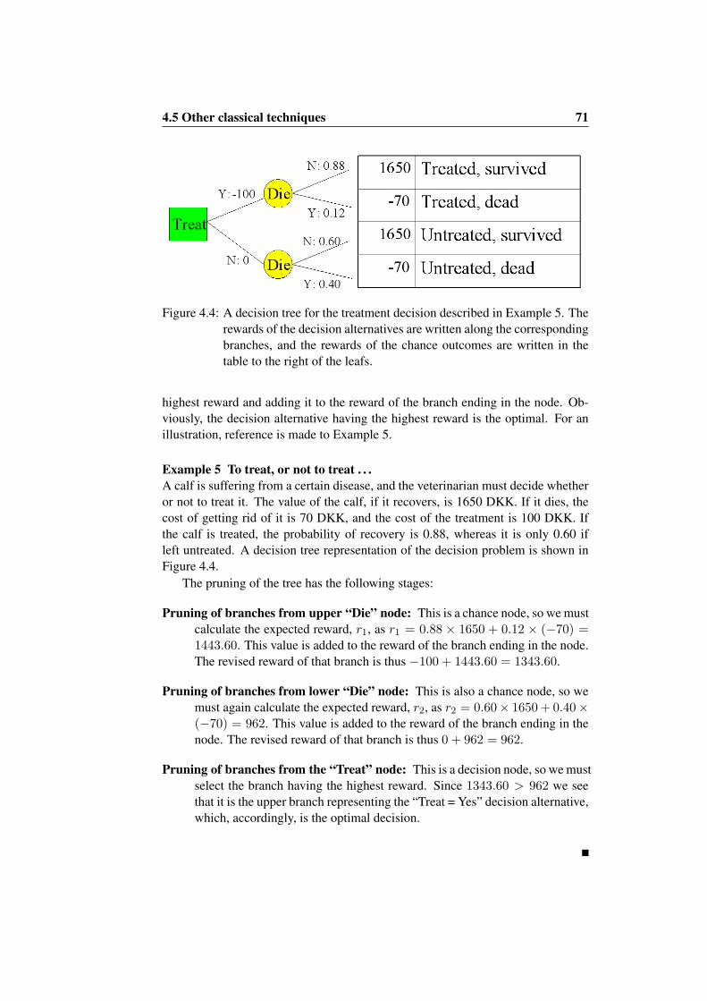
4.5 Other classical techniques 71
Figure 4.4: A decision tree for the treatment decision described in Example 5. Therewards of the decision alternatives are written along the correspondingbranches, and the rewards of the chance outcomes are written in thetable to the right of the leafs.
highest reward and adding it to the reward of the branch ending in the node. Ob-viously, the decision alternative having the highest reward is the optimal. For anillustration, reference is made to Example 5.
Example 5 To treat, or not to treat . . .A calf is suffering from a certain disease, and the veterinarian must decide whetheror not to treat it. The value of the calf, if it recovers, is 1650 DKK. If it dies, thecost of getting rid of it is 70 DKK, and the cost of the treatment is 100 DKK. Ifthe calf is treated, the probability of recovery is 0.88, whereas it is only 0.60 ifleft untreated. A decision tree representation of the decision problem is shown inFigure 4.4.
The pruning of the tree has the following stages:
Pruning of branches from upper “Die” node: This is a chance node, so we mustcalculate the expected reward, r1, as r1 = 0.88 × 1650 + 0.12 × (−70) =1443.60. This value is added to the reward of the branch ending in the node.The revised reward of that branch is thus −100 + 1443.60 = 1343.60.
Pruning of branches from lower “Die” node: This is also a chance node, so wemust again calculate the expected reward, r2, as r2 = 0.60× 1650 + 0.40×(−70) = 962. This value is added to the reward of the branch ending in thenode. The revised reward of that branch is thus 0 + 962 = 962.
Pruning of branches from the “Treat” node: This is a decision node, so we mustselect the branch having the highest reward. Since 1343.60 > 962 we seethat it is the upper branch representing the “Treat = Yes” decision alternative,which, accordingly, is the optimal decision.

72 4.6 Classical replacement theory
4.6 Classical replacement theory
In economics, the term replacement covers the decision to take an existing “asset”out of production and instead use a new one with essentially the same functions.The asset can be any factor being used over several stages. Examples include farmbuildings, inventory, sows, dairy cows, slaughter pigs etc.
Usually, we regard the present asset as a single item in a chain of assets succes-sively replacing each other. If the time horizon of production is known and fixed,the number of assets in the chain will be final. In many cases, however, the time fortermination of production will be unknown - it is just known to be “far” away inthe future. It may then be relevant, as an abstraction, to consider the present assetas the first in an infinite chain of assets. The infinite chain assumption has severalcomputational advantages as we shall see later.
The optimal time for replacement may be determined by the technical prop-erties of the asset, simply because it is not able to produce anymore. A trivialexample is light bulbs that typically produce light at a constant level, but suddenlyfail. Another example could be a sow or a dairy cow that dies. Most often, however,the asset is still able to produce (at least to some extent). It is therefore replacedbecause the new asset is expected to contribute more to the total utility value ofproduction.
In the following subsections, the classical replacement theory is briefly intro-duced. One of the first to describe the replacement problem systematically wasPreinrich (1940), but later several textbooks have described the concepts, so for amore detailed description, reference is made to such books (e.g. Rapp, 1974).
4.6.1 Replacement with identical assets
Initially, we shall assume that we are dealing with an infinite chain of identicalassets, a0, a1, . . ., where a0 is the present asset, a1 is the next etc. Our problemis to define the right moments t0, t1, . . . for replacement of each of these assets.Thus, if t0, t1, . . . are optimal, δn = tn − tn−1 is the optimal lifetime of asset n.
By “identical” we mean that the new asset is exactly as the existing one. Inother words, we assume that there is no technological or genetical improvementover time. The assumption of identical assets logically implies that the optimallifetime intervals of all assets are the same, i.e. that there exists an optimal life-time, δ, so that δ = δ0 = δ1 = . . .. Accordingly, the problem reduces to thedetermination of the optimal lifetime, δ.
For any of the assets we assume that the marginal profit at time t (when insertedinto production at time 0) is described by the function m(t). The total profit froman asset (bought at the initial priceA) over its lifetime, π(δ), is therefore calculatedas
π(δ) =∫ δ
0m(t)dt−A, (4.17)

4.6 Classical replacement theory 73
with the direct (and obvious) implication that π′(δ) = m(δ). The asset may alsohave a salvage value at time t, but for convenience, we assume that the changes insalvage value are included in m(t) (if the asset is an animal, the salvage value isthe slaughter value).
We assume that the overall aim of production is to maximize profit over time.Since we assume an infinite chain of assets, we cannot look at the total profit,because it is probably not bounded (an infinite chain is expected to give rise to aninfinite profit). In other words, it does not make sense to maximize
∑∞n=0 π(δ). A
logical alternative to total profit is to maximize average profit per time unit, a(δ).Thus, we try do identify the lifetime δ maximizing
a(δ) =π(δ)δ. (4.18)
According to standard mathematical principles we find a maximum of a func-tion by differentiation and putting equal to zero. In other words, we wish to find aδ satisfying:
a′(δ) = 0 ⇔ddδ
π(δ)δ = 0 ⇔
π′(δ)δ − π(δ)
δ2 = 0 ⇔π′(δ) = π(δ)
δ ⇔m(δ) = a(δ) .
(4.19)
From Eq. (4.19) it is seen that the optimal lifetime is found where the marginalprofit equals the average profit.
Intuitively, this makes good sense: As long as the marginal profit of keepingthe asset is higher than the average profit, it should be kept. As long as the benefitof keeping the asset for an additional time unit is higher than the average, keepingit will logically increase the average profit per time unit.
Example 6 Sow replacementApplication of the general replacement theory for sows is straight forward. Basedon data from a sow herd, Toft and Jørgensen (2002) showed that the litter sizeprofile of sows (average number piglets p(n) for parity n) in a given herd may bedescribed by the model
p(n) = −θ1 exp(−(n2 − 1)θ2) + θ3 − θ4n, (4.20)
where θ1, θ2, θ3 and θ4 are parameters to be estimated from herd data. The functionp(n) together with assumptions regarding mortality, slaughter value of sows (as afunction of age), feed consumption and prices determine the marginal and averageprofit curves, and under realistic assumptions, the results are as shown in Figure4.5.
As it is seen from the figure, the optimal replacement time is after 7th farrow-ing.

74 4.6 Classical replacement theory
Figure 4.5: Marginal and average profit (DKK) for a sow. The optimal lifetime,δ, is found at the intersection of the two curves. Under the conditionsused, the sow should be replaced after 7th farrowing.
Even though Figure 4.5 refers to sows, the course of the marginal and averagecurve is typical for many replacement problems. The initial low values for bothcurves are due to the initial replacement costs (the difference between the marketprice of the new asset and the salvage value). The growth of both curves reflectsthat a new asset typically has a high productivity and low maintenance costs. Aftersome time the productivity decreases, and the maintenance costs increase. Ac-cordingly, the marginal profit (and with some delay also the average profit) startsdecreasing.
4.6.2 Optimal replacement using discounting
In the previous subsection we used a criterion maximizing average net profit pertime unit. In economics, however, a more usual criterion of optimality is to max-imize the present value of expected future profits. As described in a previoussection, the present value p0 (at time 0) of a profit p earned at time t is simplyp0 = e−rtp, where r is the interest rate. Since, for r > 0, we have, 0 < e−rt < 1,the infinite sum of present values will actually converge to a fixed value.
The present value of the total profit over the lifetime of an asset at the time ofinsertion (time 0) is

4.6 Classical replacement theory 75
π0(δ) =∫ δ
0e−rtm(t)dt−A, (4.21)
implying that π0′(δ) = e−rtm(t). Denote as c(r, δ) a constant profit stream(money per time unit) resulting in exactly the same present value over δ time units.Clearly, c(r, δ) must satisfy
π0(δ) =∫ δ
0e−rtc(r, δ)dt = c(r, δ)
∫ δ
0e−rtdt. (4.22)
Solving Eq. (4.22) for c(r, δ) yields (by solution of the integral)
c(r, δ) =π0(δ)∫ δ
0 e−rtdt
=rπ0(δ)
1− e−rδ. (4.23)
Now, let p0(δ) be the total present value of the entire chain calculated at thetime of insertion of asset 0. We have
p0(δ) =∞∑
n=0
e−rδnπ0(δ) = π0(δ)∞∑
n=0
(e−rδ
)n=
π0(δ)1− e−rδ
. (4.24)
The last equal sign of Eq. (4.24) uses the well known mathematical fact thatfor 0 < q < 1 we have
∑∞i=0 q
i = 1/(1 − q). In order to decide on an optimallifetime, δ, we differentiate and put equal to zero:
p0′(δ) = 0 ⇔ddδ
π0(δ)1−e−rδ = 0 ⇔
π0′ (δ)(1−e−rδ)−π0(δ)re−rδ
(1−e−rδ)2= 0 ⇔
π0′(δ)(1− e−rδ)− π0(δ)re−rδ = 0 ⇔π0′(δ) = π0(δ)re−rδ
1−e−rδ ⇔e−rδm(δ) = c(r, δ)e−rδ ⇔
m(δ) = c(r, δ) .
(4.25)
Since c(r, δ) is a kind of generalized average profit per time unit, we see thatalso when we use discounting, the optimal replacement time δ is found where themarginal profit equals average profit.
4.6.3 Technological or genetical improvement
In this subsection, we will not assume anymore that the assets of the infinite chainare completely identical. Instead we shall assume that future assets in some senseare better than the present one. This is a rather realistic assumptions due to techno-logical or genetical improvements over time.

76 4.6 Classical replacement theory
In order to solve the problem under such conditions, we need to make an as-sumption concerning the nature of the improvement. We shall denote the marginaland total profit function of the nth asset in the chain as mn(t) and πn(δ), respec-tively. A linear improvement means that the marginal profit function (where t = 0is the time of insertion) is of the form
mn(t) = αδn+m0(t), (4.26)
where α is the increase per time unit. An exponential improvement leads to themarginal profit function
mn(t) = eβδnm0(t), (4.27)
where β is the relative increase per time unit. Thus, β = 0.01 implies that themarginal profit (from new assets) increases by 1 percent per time unit. In the fol-lowing we shall investigate the exponential form and its consequences. It followsdirectly from (4.27) that
π0n(δ) = eβδnπ0
0(δ). (4.28)
Our criterion for determination of the optimal lifetime is now (like the previoussubsection) that we wish to maximize the present value p0(δ) of the entire chain,where
p0(δ) =∞∑
n=0
e−rδnπ0n(δ) =
∞∑n=0
e−rδneβδnπ00(δ) = π0
0(δ)∞∑
n=0
e(β−r)δn. (4.29)
By use of the rule∑∞
i=0 qi = 1/(1− q) we end up with
p0(δ) =π0
0(δ)1− e(β−r)δ
. (4.30)
In order to decide on an optimal lifetime, δ, we differentiate and put equal tozero:
p0′(δ) = 0 ⇔ddδ
π00(δ)
1−e(β−r)δ = 0 ⇔π0′0 (δ)(1−e(β−r)δ)+π0
0(δ)(β−r)e(β−r)δ
(1−e(β−r)δ)2= 0 ⇔
π0′0 (δ)(1− e(β−r)δ) + π0
0(δ)(β − r)e(β−r)δ = 0 ⇔π0′
0 (δ) = −π00(δ)(β−r)e(β−r)δ
1−e(β−r)δ ⇔e−rδm0(δ) = c(r − β, δ)e(β−r)δ ⇔
m0(δ) = c(r − β, δ)eβδ .(4.31)

4.6 Classical replacement theory 77
Figure 4.6: Optimal replacement time for sows with and without genetical im-provement. The curve marked as “No improvement” is the functionc(r, δ) as defined in Eq. (4.23), whereas the one marked as “Improve-ment” is the function c(r − β, δ)eβδ as shown in Eq. (4.31). Geneticalimprovement implies earlier replacement.
Under usual conditions, c(r − β, δ)eβδ > c(r, δ) implying that the optimallifetime of the present asset is lower when technological or genetical improvementsare assumed.
Example 7 Sow replacement with genetical improvementIn Figure 4.6 the discounting criterion is used for the sow replacement problemintroduced in Example 6. An annual interest rate of 5% is assumed. The figureshows the optimal replacement time without genetical improvement compared to asituation with an annual improvement of 1%.
As it is seen from the figure, the optimal replacement time under the discount-ing criterion is the same as the one in Figure 4.5 (after 7th farrowing) as long asgenetical improvement is ignored. Adding a 1% annual genetical improvementshifts the optimal replacement time to the left.
4.6.4 Limitations and applications of the classical replacement theory
The classical replacement theory provides us with a general framework for dealingwith optimal lifetime of assets. It has, also under practical farm conditions, many

78 4.6 Classical replacement theory
Figure 4.7: Average and marginal profit of a dairy cow over parities. There is anintersection between the curves in each lactation.
areas of application. It is well suited for all kinds of machinery, and, to some extent,optimal slaughter time for broilers, bull calves and slaughter pigs. It has also somerelevance for the sow replacement problem, and (within lactation) the dairy cowreplacement problem.
In general, the main limitations may be summarized as:
Uncertainty: The classical replacement theory assumes full certainty about themarginal profit function, the investment costs and all prices. As discussed indetails in Chapter 2, uncertainty is an inherit property of the decision makingprocess in herd management. The uncertainty is partly a consequence ofimperfect knowledge, and partly of random variation.
Uniqueness: The general theory implicitly assumes that the marginal and averageprofit functions are as shown in Figure 4.5 with a uniquely determined inter-section. For several applications the intersection is not unique. This is, forinstance, the situation in dairy cows, where the average and marginal profitsare as shown in Figure 4.7.
Availability: The theory assumes that a new asset for replacement is always avail-able.
For several of the areas mentioned, the limitations are not so serious that themethod cannot be used. When dealing with the animal replacement problem, sev-eral characteristics of the problem are problematic in relation to the theory as de-scribed already by Ben-Ari et al. (1983). Those characteristics are:

4.7 Exercises 79
Uniformity: The traits of animals are difficult to defined and measure. Therefore,the true state of the factor (the animal) is typically not known with certainty.
Variability: The traits of animals vary considerably among animals as well as overtime for the same animal.
Reproductive cycle: For some animals (in particular dairy cows), the reproduc-tive cycle makes the replacement problem two dimensional. It must be de-cided in which lactation to replace the animal and at what stage inside lacta-tion.
Herd constraints: Often the replacement decision for an individual animal is notindependent of decisions made for other animals due to herd constraints.Obvious examples include:
Availability of replacement animals: Most often there is a limited supplyof e.g. heifers or gilts for replacement.
Production quotas: If for instance a dairy herd produces under a milk quota,the decision to cull one cow influence the ability of the whole herd tomeet the quota.
Batch production: In slaughter pigs, for instance, no new piglets are in-serted into the pen before it is empty. The principle may even be ap-plied on section level. The slaughter decision therefore has two dimen-sions: When to slaughter individual pigs, and when to terminate thebatch by sending the remaining pigs to the slaughterhouse.
Due to the characteristics listed, the standard method for dealing with theanimal replacement problem has become dynamic programming (also known asMarkov decision processes) in recent years. For a survey of such techniques, ref-erence is made to Kristensen (1994).
Despite the limitations, there are (in particular in older research) many exam-ples of application of the classical replacement theory in animals. For a surveyin relation to dairy cows, reference is made to van Arendonk (1984). In sows,Dijkhuizen et al. (1986) has used the technique.
4.7 Exercises
4.7.1 Gross margin
A dairy farmer has housing facilities for 110 dairy cows, and the size of his milkquota is 650,000 kg milk. During the last quota year he had on average 100dairy cows. His total milk production amounted to 680,000 kg milk (deliveredto the dairy). During the year he sold 45 dairy cows and received total a paymentof 320,000 DKK. A total of 110 healthy calves were born and 46 heifers werebought/transferred.

80 4.7 Exercises
For feeding of the cows the farmer used 213,100 SFU of concentrates and340,000 SFU of roughage. Various costs for bedding, breeding, veterinary servicesetc amounted to 113,400 DKK. A permanently employed herdsman has been paid300.000 DKK whereas interests and depreciation costs of the housing facilitieswere 300,000 DKK.
Relevant prices were:Milk, DKK per kg, 2.75Calves, DKK per calf, 1250.00Heifers, DKK per animal, 8000.00Concentrates, DKK per SFU, 1.95Roughage, DKK per SFU, 1.25Quota penalty, DKK per kg mil above the limit, 2.70
a Calculate the gross margin (net returns to housing, labor and management)per cow per year
b Calculate the gross margin (net returns to housing, labor and management)per kg quota milk
c Which of the two gross margins is relevant in the herd in question?
d What is meant by “gross margin”? What is the difference between grossmargin and net profit?
4.7.2 Internal prices
A dairy farmer considers whether he shall grow beets for winter feeding or he shallbuy industrial by-products instead. If he chooses not to grow beets he intends togrow spring barley on the field in question instead. In that case, the barley will besold. The farmer has made the following calculation of the costs and revenues ofgrowing beets and barley (all figures are per hectare):
Barley BeetsSowing costs, DKK 427 576Fertilizer, DKK 889 2291Chemicals, DKK 260 1270Drying costs, DKK 358 0Plastic, DKK 0 43Fuel, cultivation, machinery, DKK 4060 6520
Yield, hkg grain 64 0Yield, hkg straw 40 0Yield, SFU 0 12,500
Value of grain, DKK per hkg 124 -Value of straw, DKK per hkg 20 -

4.7 Exercises 81
Figure 4.8: Milk yield as a function of energy intake (fixed level of protein and fat).
a Calculate the gross margin of spring barley.
b Calculate the internal production price for beets.
c Shall the farmer grow beets if industrial by-products with exactly the samenutritional content can be purchased for 1.00 DKK?
4.7.3 Marginal considerations, I
At fixed level of crude protein and fat, the relation between energy intake (SFU)and milk yield of dairy cows was found to be
Y = −27.94 + 6.546X − 0.212X2, (4.32)
where Y is daily milk yield andX is the daily energy intake. The function is shownin Figure 4.8.
It is assumed that there is no limited quota.
a Indicate directly in Figure 4.8 the marginal increase in milk yield if the en-ergy intake is increased from 14 to 15 SFU.
b Calculate the marginal increase in milk yield at the exact energy intake X =14 SFU. Illustrate in Figure 4.8.
c Determine the optimal energy intake under the assumption that the price ofan additional energy unit is 1.60 DKK and the price of a kg milk is 2.60DKK.

82 4.7 Exercises
d What determines the optimal energy intake, under the assumption that theproduction function (the relation between the factor X and the product Y isas shown in Figure 4.8?
e Why is it necessary to assume that there is no quota?
4.7.4 Marginal considerations, II
Bull calves fed ad libitum are assumed to consume the following number of energyunits (SFU) per day:
X = 3.56 ln(W )− 13.61, (4.33)
where X is daily energy intake (SFU) and W is the weight in kg. The correspond-ing daily gain G (kg per day) is assumed to be:
G =X
2.17 exp(0.00256W )(4.34)
It is assumed that the housing capacity is “unlimited”, that the slaughter priceis 12.00 DKK per kg live weight and the feed price is 1.50 DKK per SFU.
a Describe how to find the optimal slaughter weight of bull calves. Use forinstance a spreadsheet to determine it.
b Why is it necessary to assume that the housing capacity is “unlimited”?
4.7.5 Investments
A pig farmer buys new equipment for 500,000 DKK. It is expected to be used forthe next 10 years and the interest rate is 12%.
a What is the annual cost of the investment?
b In what way does it matter whether the farmer:
• already has the money in the bank?
• has to borrow the money in the bank?
• borrows the money from his rich uncle?
c What does deprecation mean?

Chapter 5
Basic production monitoring
This chapter presents the theory behind traditional production monitoring systemsbased on production reports presenting a number of selected key figures. Laterchapters will introduce more advanced methods for production monitoring.
5.1 The framework
With reference to the herd management cycle shown in Figure 1.1, productionmonitoring covers the steps “Check” and “Analysis”. In Figure 5.1, the elementsrelating to monitoring are shown in an expanded version.
The “Check” is basically a comparison of the results achieved in productionwith some predefined target values. The target values are a result of the planningprocess, and they are in principle of the same nature as the “goals” shown in Figure1.1. The only difference (if any) is that the targets are very specific and directlycomparable with the key figures calculated from a (more or less continuous) flowof registrations of events relating to the factors or the products. Examples of keyfigures (and corresponding targets) are conception rate, average daily gain, averagedaily milk production, average litter size etc.
The result of the check is binary: Either is the result at least as good as thetarget value or it is not. In case of a negative outcome (the result is not as good asthe target value), an analysis should be carried out. It consists of two elements:
1. Is the deviation significant from a statistical point of view?
2. Is the deviation significant from a utility point of view?
If the answer to both questions is “yes”, an adjustment of the production maybe relevant.
The elements of the monitoring process may be listed as:
• Data recording
• Database

84 5.1 The framework
Figure 5.1: Expanded “monitoring part” of the management cycle.

5.2 The elements of the monitoring process 85
• Data processing
• Report with key figures
• Analysis
– Statistical
– Utility
• Decision: Adjustment/no adjustment
In modern livestock production the basic production monitoring is most oftensupported by some kind of computer program (often called a Management Infor-mation System or just “MIS”). Such system will typically have an interface forentering records (which may be partly automated) in a database, and it performsthe necessary data processing and presents a report with key figures. Sometimes thereport also contains relevant target values and even results of a statistical analysis.The utility evaluation, however, is usually not part of the system. In the followingsubsections we shall discuss the elements of the monitoring process further.
5.2 The elements of the monitoring process
5.2.1 Data recording
Recording (data registration) is usually related to events in production. An eventis when “something” happens. Examples of events in a sow herd include mating,farrowing, weaning, moving etc. In a dairy herd, events also include for instancetest of milk production at cow level, and, in automatic milking systems, we mayeven consider milking as an event with associated recording. A precise definitionof a record (the result of a data registration) is shown in Definition 6 together withan actual example of a record registered in a sow herd (Example 8).
Definition 6 A record, ρ, is defined by the following properties:
Event, ρ.e: What does the record relate to?
Identification, ρ.i: The unique number of the animal(s)/section/batch in question.
Registration level, ρ.l: Is it on animal/pen/section/batch/herd level?
Time, ρ.t: Date (or date and time).
Property, ρ.p: What is measured?
Value, ρ.v: The numerical or categorical value actually measured.

86 5.2 The elements of the monitoring process
Example 8 An actual record from a sow herd.Property ValueEvent ρ.e = “Farrowing”Identification ρ.i = “Sow #1234”Registration level ρ.l = “Animal level”Time ρ.t = “February 1st, 2006”Property ρ.p = “Live-born piglets”Value ρ.v = 12
The traditional registration method is paper and pencil, but in recent years alsodifferent kinds of electronic equipment has become available for data recording.
5.2.2 Database
The individual records collected over time are typically entered into a database.A (relational) database is organized as a collection of interrelated tables. Properdesign of a database (i.e. what tables to define and how to interrelate them) isnot a trivial task, but, for the ordinary user it is not necessary to master the art ofdatabase design. Readers who are interested in the subject may consult a textbookas for instance Watson (2002).
Even though most MISs provide automatically generated production reportswith key figures it is important to know the principles behind the use of a database.Such knowledge will enable the user to make more detailed and/or more special-ized analyses of the production than those provided by the MIS.
The communication with the database is usually done by use of the StructuredQuery Language (SQL) which is a common standard for describing and queryingdatabases. It is available with many commercial relational database products, in-cluding DB2, Oracle and Microsoft Access (Watson, 2002). Most MISs rely on astandard commercial database, implying that it can be accessed by usual statisticalsoftware tools like SAS or R. Occasionally it happens that the manufacturer of theMIS has blocked the database for external communication by password protectingit. Such limitations should not be accepted by farmers.
A typical way of organizing the database is by collecting records relating tothe same event in a table. Thus, the database typically has a table for each eventconsidered. Example 9 shows a table for the event “Farrowing” in a sow herd. Typ-ically each property of a record (cf. Definition 6) either corresponds to a column inthe table, or, it is a general property of the table as such. In the example, there arecolumns for “Identification” (Sow #), “Time” (Date) and “Property” (Live-born),whereas “Event” and “Registration level” are general properties of the table (it is atable for the event “Farrowing” and all records are at animal level).

5.2 The elements of the monitoring process 87
Example 9 A table in the database of a sow herd.Sow # Date Live-born Stillborn Course1234 15 January 2006 12 2 Easy678 16 January 2006 9 4 Diff.1001 18 January 2006 14 1 Easy. . . . . . . . . . . . . . .. . . . . . . . . . . . . . .. . . . . . . . . . . . . . .
It should be noticed that each row in the table actually contains informationabout 3 different records, but, all relating to the same event (“Farrowing”). Theexample assumes that 3 properties (cf. Definition 6) are measured for the event“Farrowing”: Number of live-born piglets, number of still-born piglets, and thecourse of the farrowing as a categorical value (either “Easy” or “Difficult”). Sincethe number of total born piglets is a simple sum of live-born and stillborn, a sepa-rate column for “Total born” will typically be omitted in order to avoid redundantinformation in the database.
The database as such may be regarded as a collection of tables, where eachtable typically relates to an event.
5.2.3 Data processing
The data processing dealt with here corresponds to the first processing shown inFigure 2.1. In this chapter the description will be kept at a basic level in agree-ment with traditional monitoring systems. A description of the path from data toinformation at a more advanced formal level will be given in Chapter 6.
Referring to Figure 2.1, the information resulting from the processing in thetraditional basic setup is a number of selected key figures characterizing the effi-ciency of production. The final decision at the end of the path is whether or not tomake adjustments (and what kind of adjustments).
The purpose of the processing is data reduction. In principle all informationabout the herd is already present in the database, but nobody will be able to interpretit unless it is reduced to a dimension that can be over viewed by the decision maker.
The key figures will typically refer to a specific period, i.e. the most recentmonth, quarter or year. What the MIS actually does in order to obtain the keyfigures is to ask questions to the database (using the SQL language). The answersare then further processed into simple or more complex key figures. In Table 5.1 thecalculation of a few selected key figures for a sow herd is shown. It is obvious, thatif registrations of relevant events like farrowing, mating, and pregnancy diagnosishave been performed, the answers to the questions are easily found in the database.Readers, who are interested in the syntax of the SQL language, used for askingquestions, may for instance consult Watson (2002).
In some cases, the questioning of the database and the subsequent processingmay be more complex. As an example, we shall use the key figure “Average daily

88 5.2 The elements of the monitoring process
Table 5.1: Examples of simple key figures for a sow herd. The key figures areassumed to refer to a period of w weeks.
Key figure Question asked to the database Answer FormulaFarrowings perweek
How many farrowings were there in theperiod?
f f/w
Matings perweek
How many matings were there in theperiod?
m m/w
Live-bornpiglets per litter
How many piglets were born in the pe-riod?
p p/f
How many farrowings were there in theperiod?
f
Conception rate How many matings were there in theperiod?
m d/m
How many positive pregnancy diag-noses were there in the period?
d
gain” in slaughter pigs. In commercial production systems, slaughter pigs are notindividually identified. The straightforward calculation of individual gain frominsertion to slaughter followed by calculation of the average value per day cantherefore not be used. Instead an indirect method based on valuation weighing isoften used. The principles are shown in Example 10.
Example 10 Calculation of average daily gain in slaughter pigs.When the pigs are not individually identified the total gain for a certain period maybe calculated as follows:
+ Total weight, slaughtered pigs ws
+ Total weight, dead pigs wd
+ Valuation weight, end of period ve
− Total weight, piglets inserted wi
− Valuation weight, beginning of period vb
= Total gain during the period gt
By “valuation weight” we mean the total weight of all slaughter pigs being presentin the herd on a particular day. In order to arrive at the average daily gain, the totalgain gt must be divided by the total number of days in feed, d, in the period. Thus,the average daily gain g is g = gt/d.
In order to retrieve the values used for calculation of gt we must have tables inthe database for the events “Slaughtering”, “Death”, “Insertion” and “Valuation”.Based on the tables for slaughtering, death and insertion we may at any day of theperiod calculate the number of pigs present in the herd. The sum of those numbersover all days of the period will provide us with the number of days in feed, d.

5.2 The elements of the monitoring process 89
It should be emphasized, that for any rational interpretation of the key figures,it is necessary to know exactly how it is calculated, and what records it is based on.Such information is usually given in the documentation provided by the manufac-turer of the MIS. If that is not the case, the farmer shouldn’t buy it!
5.2.4 Report with key figures
If a MIS is used for the monitoring process, the key figures shown in the reportare often more or less predefined even though some systems allow for selection offigures to be presented and thus provide a limited degree of flexibility.
Usually the report contains (too) many key figures and it may even be a problemfor the farmer to choose the most relevant for closer evaluation. In the followingsubsections, the principles for choosing the best key figures and for interpretationwill be described.
Types of key figures
The purpose of key figures is to provide the farmer with a condensed set of infor-mation expressing the current state of the production. Many different kinds of keyfigures each expressing certain aspects of production can be defined. In general,we distinguish economical key figures from technical key figures. Whereas thefirst are expressed in money, the latter are expressed in product or factor units (orratios). In this book, we shall mainly discuss technical key figures. Typically theyattempt to express one of the following basic properties:
Productivity: Such key figures express the average production level of a productper time unit. Let Yt = (Y1t, . . . , Ynt)′ be the vector of n products producedat stage t. If we wish to express the productivity of product i in the periodfrom stage t− k to stage t, we may simply calculate the productivity πit as
πit =1k
t∑τ=t−k
Yiτ (5.1)
Typical examples of key figures expressing productivity include “piglets pro-duced per week”, “average daily milk production” etc.
Factor consumption: This is just the counterpart of productivity. Let xt = (x1t, . . . , xmt)′
be the vector of m factors consumed at stage t. The average consumption citof factor i in the period from stage t− k to stage t, is calculated as
cit =1k
t∑τ=t−k
xiτ (5.2)
Even though key figures in this category are rare, examples could be “feedconsumption per month”, “average number of cows” etc.

90 5.2 The elements of the monitoring process
Technical efficiency: Technical efficiency expresses the ratio of a product to afactor. Using the same notation as before, the key figure κijt expressing theefficiency of the production of product i relative to the consumption of factorj is calculated as
κijt =πit
cjt=∑t
τ=t−k Yiτ∑tτ=t−k xiτ
(5.3)
Key figures expressing technical efficiency are probably the most commonlyapplied and they include so well known properties as “milk yield per cow peryear”, “piglets per sow per year”, “gain per feed unit” in slaughter pigs/calvesetc. If we extend the definitions of factors and products to cover also inputand output of sub-areas of the production process, even key figures as forinstance “conception rate” (factor = insemination, product = pregnancy) fallinto this category.
The only economical key figures we shall briefly discuss here are those ex-pressing gross margins. They may be calculated as total figures, or relative to amain factor or a main product. In dairy herds, for instance, we may calculate grossmargin per cow per year and/or gross margin per kg of milk produced. In general,relative values should be calculated relative to the most limiting constraint. Thus,if the dairy farmer produces under a quota, the most relevant figure is gross marginper kg of milk (if the the quota is the most limiting constraint). In the absence ofa quota, it is more relevant to consider gross margin per cow per year, because inthat case, the housing capacity is assumed to be the most limiting constraint.
Key figures and their interrelations
Even though the production report may contain many different key figures, it isimportant to realize that many are heavily correlated. In order to illustrate theinterrelations, a collection of typical technical key figures for a sow herd are shownin Figure 5.2. They are all examples of commonly defined properties used forcharacterizing a sow herd.
A sow herd has one well-defined main product which is piglets (sold on themarket or kept for fattened by the farmer himself). Therefore, the over-all produc-tivity of the sow herd is expressed well by the key figure “piglets sold per year”.This key figure is shown at the top of the diagram, and with that as a starting point,a tree of key figures has been created by simple logical reasoning. The principle isthat an arrow between two key figures indicates a causal influence. Starting fromthe top, the figure illustrates that the number of piglets sold is influenced (in thiscase determined) by the number sold per sow (an efficiency key figure) and thenumber of sows (a factor consumption key figure) and so on downwards. In gen-eral, all key figures below a certain position in the tree have an explanatory effecton the value at the position in question.

5.2 The elements of the monitoring process 91
Figure 5.2: Typical key figures (rectangles) of a sow herd. Ellipses indicate deci-sions made by the manager. The arrows indicate interdependencies.

92 5.2 The elements of the monitoring process
The figure illustrates that the over-all productivity in a sow herd may be ex-plained by a large number of effects that basically can be split up into 4 distinctgroups as the symbols indicate. The groups are:
• Litter size productivity.
• (Foetus and) piglet mortality.
• Reproductive efficiency.
• Housing system utilization efficiency.
Whereas the various key figures for litter size productivity are (logically) heav-ily inter-correlated, the 3 key figures for mortality are not logically inter-correlated(i.e. there are no arrows between them). They may, however, often be biologicallyinter-correlated in the sense that if a herd has a high piglet mortality, it is probablybecause of bad management, disease pressure etc. It is therefore likely that thesame applies to weaners with a corresponding high mortality as a consequence.
As concerns the key figures for reproductive efficiency, the “root” of the sub-tree covering those figures, “litters per sow per year” represents a kind of totalproductivity concerning reproduction. The figures closer to the leaves of the treeaccordingly represent explanations for the over-all reproductive efficiency. Pro-ceeding to the leaves, the overall efficiency is split up into properties relating to thesows (“conception rate” and “days from weaning to oestrus”) and one relating tothe staff (“oestrus detection rate”).
In the selection of key figures to monitor with particular care, the general adviceis to select a few that are not (or only slightly) correlated. For the productivity in asow herd it would be natural to choose one from each of the 4 groups identified inFigure 5.2.
It should be emphasized that the principles of Figure 5.2 where very aggregatedproperties (on the top) are explained by more specific underlying properties maybe applied to any livestock production and to some extend also for key figuresmeasuring factor consumption. It is left to the reader as an exercise to construct asimilar figure for productivity in a dairy herd.
Properties of key figures
In the interpretation of calculated key figures, at least three properties are relevant:
Correctness: This property deals with the observation that the data registrationsbehind it must all be correct. From a theoretical point of view, the observa-tion is trivial, but, from a practical point of view it is certainly not. Numerouserrors may occur under the registration of data: The identification may bewrong (an observed insemination or farrowing may be ascribed to a wrongsow), registrations may be lost or forgotten, values may be misread etc.

5.2 The elements of the monitoring process 93
Validity: The validity of a key figure expresses to what extent it gives us the de-sired information. As discussed in Section 2.3.1 we often want to knowsomething that is not directly observable. We are therefore forced to observeor calculate something that is related to the desired property. It is, however,not the same. If it is “close” to the desired property, the validity of the keyfigure is “high”. If it is only slightly related to the desired property, the va-lidity is “low”. These vague terms illustrate that we are usually not able tocalculate a numerical value for the validity, but, only use a crude classifica-tion. It must be emphasized that the validity is not an absolute property of akey figure. It only makes sense when relating the key figure to a well defineddesired information. In other words, the same key figure may have “low”validity in relation to one desired information and high in relation to anotherkind of information.
Precision: The precision expresses the certainty by which the key figure has beendetermined. We may regard the calculated value as an estimate (in statisticalsense) of a true underlying value. A formal definition is given in Definition7.
Definition 7 Precision of a key figure: Let the key figure κ be an estimateof an underlying true value θ estimated on the data set D using a knownestimation technique resulting in an unbiased estimate (i.e. E(κ) = θ) withthe standard deviation σ so that V(κ) = σ2. The precision of the key figureτ is then
τ =1σ2. (5.4)
In other words, the precision of a key figure is an absolute numerical value.It is one of the most important properties at all to consider when we interpretkey figures. From the definition it is clear, that if a large data set D is avail-able (i.e. it is a big herd), the precision will typically be high as we shall seelater.
Even though Definition 7 is the correct and formal, we will often use thestandard deviation σ as a direct expression for the precision. In that case,low values of σ correspond to high precision and vice versa.
Correctness
It is in practise very difficult to actually guarantee that the registrations behind akey figure are correct. This is simple a consequence of the fact that errors mayoccur in so many different ways that it is more or less impossible to foresee all ofthem.

94 5.2 The elements of the monitoring process
What a MIS typically does in practise is to run some automatic checks ofrecords. Examples of such checks are given in Example 11. As it is seen, suchverification checks are often trivial, but nevertheless, they are very useful. Thestrength is that records that are obviously wrong are identified, but there is cer-tainly no guarantee that records passing the tests are correct. If they are wrong,but not unusual, they will pass. To decide the acceptance limits of the checks is atradeoff between the wish to identify wrong values and to avoid discarding recordsthat are actually correct (even though they may be extreme). It is, for instance, nottrivial to decide on an absolute maximum for a litter size to be accepted.
Example 11 Typical verification checks for a data record ρ (with fields as in Def-inition 6) from a sow herd.
Event, ρ.e Property, ρ.p Verification checkFarrowing Litter size 0 ≤ ρ.v < 25Farrowing (Any) A mating record exists for the same sowMating (sow) (Any) A weaning record exists for the same sowWeaning Weight of piglets 5n < ρ.v < 10n, (n = number of piglets)
Another kind of verification check typically done is to create a kind of balanceaccounting for all animals present in the herd. If a valuation has been carried outon a certain historic date, and records of all animals born, bought, sold or dead arekept, a balance as illustrated in Example 12 may be created.
Example 12 Balance accounting for all animals in a slaughter pig unit.+ Slaughter pigs in the unit, previous valuation day np
+ Weaners bought since previous valuation day nb
− Dead slaughter pigs since previous valuation day nd
− Sold slaughter pigs since previous valuation day ns
= Slaughter pigs present in the unit today nt
The number of pigs present in the unit (determined by counting) must match thecalculated number nt in order for the records to be correct.
Again, even though the balance check of Example 12 is extremely useful inpractise, passing it still doesn’t guarantee that the records are correct. Passing is anecessary condition for correct records, but it is certainly not a sufficient condition.Nevertheless it is a simple, but effective, method for checking that “all” events havebeen registered.
To sum up, several verification checks can be defined, but only care with reg-istrations can ensure that the records behind a key figure are correct.
Validity
Of the three basic properties of key figures, validity is probably the most difficultto understand. In order to improve the understanding of the concept, we shall take

5.2 The elements of the monitoring process 95
a look at few examples (more examples can be found in the exercises of Section5.3.
Suppose that we wish to describe the reproductive efficiency of a sow herd byone single key figure. The question is then which one we should choose. Referringto Figure 5.2, it is obvious that we should search among those shown on a greybackground. Let us take a look at each of them one by one and assess their validity:
Litters per sow per year: If what we really wish to know is something about theover-all reproductive efficiency of the sow herd, this figure has a rather highvalidity. It is, however, also influenced by the weaning and culling policyof the pig farmer. Since the weaning and culling policy has nothing to dowith the reproductive efficiency, it decreases the validity. If these policiesare constant over time, changes in the value of the key figure reflect changesin reproductive efficiency. Thus for within farm use, the validity is high,but if key figures for different farms are compared, the validity is lower, be-cause the weaning and culling policies probably vary among farms. Even forwithin-farm use, the key figure is rather unspecific. If the value decreases, itis not possible to know whether it is because of, for instance, low conceptionrate or low oestrus detection rate.
Weaning age: This is almost entirely a consequence of the weaning policy of thefarm. Thus, the validity as an expression for reproductive efficiency is ex-tremely low.
Non-productive days: This key figure is very often used as an expression for re-productive efficiency. It has a higher validity than “litters per sow per year”,because it does not depend logically (but slightly biologically) on the wean-ing policy. There is, however, still a marked influence of the culling policy(if re-maters are always culled, the number of non-productive days will de-crease).
Days from weaning to oestrus: This is a rather specific key figure attempting tomeasure a property of the sows in the herd. Regarded as an expression for thestate of the sows, the validity is decreased by the fact, that what is measuredis detected oestrus. The value is therefore also influenced by the oestrusdetection rate which is a property of the farmer.
Conception rate: An attempt to measure the ability of the sows to conceive. Thevalue also expresses the efficiency of the inseminations (timing, stimulation,procedure) thus reducing the validity as an expression for a property of thesows.
Percent re-mating: A very composite key figure combining effects of conceptionrate, oestrus detection rate and culling policy. The validity (for almost anypurpose) is therefore low.

96 5.2 The elements of the monitoring process
Oestrus detection rate: An attempt to measure the ability of the staff to detectheat. It is not used very often in pig herds (whereas it is commonly appliedin dairy herds). Even a very small probability of false positive detectionsmay change the value dramatically.
The examples concerning sow herd reproduction illustrate that if a key figureis systematically influenced by aspects with no (or only little) relevance for the in-formation we wish to obtain, the validity of the key figure as source of informationis decreased. Thus, again, it must be emphasized that the concept of validity onlymakes sense in relation to specific information we request.
Precision
The standard deviation of a key figure expresses the degree of certainty of thecalculated value. The uncertainty has two sources:
The sample uncertainty: This uncertainty expresses the natural variation (oftenreferred to as the biological variation). It corresponds to the trivial observa-tion that even though the production has been conducted in exactly the sameway (i.e. exactly the same factors have been used in the same amounts) intwo periods, we nevertheless, don’t expect exactly the same result simply be-cause of the random nature of (biological) production. Mathematically, thesample uncertainty is a consequence of the random term et of the productionfunction (1.1) which is not under the control of the farmer.
The observation uncertainty: Depending on the registration methods used in or-der to obtain the records, a measurement error may be involved.
The effects of the two sources of uncertainty may be expressed by the followingmodel:
κ = θ + es + eo, (5.5)
where κ is the calculated key figure, θ is a true underlying value (which we try toestimate), es is the sample error, and eo is the observation error.
Assuming the model (5.5), the variance of the estimate is σ2 = V(es + eo).If the two error terms are independent (which they usually are), we have σ2 =V(es)+V(eo). In other words, the key to the precision is to calculate the variancesof es and eo. In many cases it is realistic to assume both error terms to be normallydistributed, i.e, es ∼ N (0, σ2
s) and eo ∼ N (0, σ2o). This is often a reasonable
assumption for continuous properties like milk yield. In other situations, the vari-ance of the key figure is the result of binomial variation, which is the case when thekey figure measures a binary output as for instance with conception rate and heatdetection rate. Also other distributions as for instance the poisson distribution maybe used.
The next section contains a number of practical examples of how to calculatethe precision.

5.2 The elements of the monitoring process 97
5.2.5 Analysis from a statistical point of view
General principles
The way in which the key figures are actually presented depends on the MIS usedin the herd. A typical way is, however, a table where each key figure is shown ina separate row containing the name of the key figure, the calculated value (perhapsfor several periods) and sometimes also a target value. An example of such a rowin a report for slaughter pigs is shown in Example 13.
Example 13 A row of a typical production report for slaughter pigsProperty Quarter t-3 Quarter t-2 Quarter t-1 Quarter t Target. . . . . . . . . . . . . . . . . .Daily gain (g) 988 934 896 925 950. . . . . . . . . . . . . . . . . .
In the example, the target value for daily gain was 950 g, but the achieved valuefor the present quarter (time t) was only 925 g. The basic question is therefore:Should we be worried? It is easily seen that the calculated gain is 25 g less thanthe expected target, but, could it be a simple consequence of random biologicalvariation and/or observation errors?
In statistical terms, the basic question is whether the calculated key figure κcould be an observation from a distribution having the mean θ′ (where θ′ is thetarget value) and the variance σ2 = V(es) + V(eo). A formal way of testing this isto test the null hypothesis
H0 : θ = θ′ (5.6)
Often, we are only worried in case of “negative” deviations from the targetvalue. It may then be relevant to use a one-sided test of the type H0 : θ ≥ θ′
instead of (5.6). Under all circumstances, if the null hypothesis is rejected, weshould be worried. The deviation of the calculated value from the target is in thatcase not likely to be the result of random biological variation and/or observationerrors.
The practical setup of the test depends on the underlying distributions implyingthat it may be relevant to distinguish between continuous and categorical proper-ties. In both cases, the most difficult part is to calculate the precision.
Even though the practical setup differs, the procedure under all circumstancesinvolves the following steps:
1. Identification of the formula(s) used for calculation of the key figure fromrecords.
2. Identification of the distributions of the data.
3. Identification of the distribution of the key figure under the null hypothesis.

98 5.2 The elements of the monitoring process
Table 5.2: Average daily milk yield (ECM) during the first 24 weeks of the lacta-tion in a herd.
Parity No. of cows Key figure Target1 10 20.4 23.5≥ 2 12 26.0 27.8
4. Calculation of confidence limits for the key figure based on the precision.
5. Acceptance or rejection of the null hypothesis.
Referring to the “key figure tree” of Figure 5.2, the procedure will typicallybe to focus on the key figures in the “leaves” of the tree. Those close to the rootare very aggregated values, where in particular identification of the distribution isdifficult.
Continuous properties
We shall illustrate the procedure for the statistical evaluation through two exam-ples concerning continuous properties: Average daily milk yield of dairy cows andaverage daily gain in slaughter calves.
Example 14 Average daily milk yieldIn the Danish management information system for dairy cows, the average dailymilk yield of the cows during the first 24 weeks of lactation is calculated for firstlactation cows and other cows, respectively. In the system, the farmer may comparethe results to his own targets (expected values). The results in a herd were as shownin Table 5.2. We observe, that the calculated result for all parities is lower thanexpected. The question is now, whether or not the deviation is significant from astatistical point of view.
Following the procedure described in last section we notice and conclude asfollows:
Calculation of the key figure from data: The basic records behind the key fig-ure are test day milk yields (including protein and fat content) at cow level.Using a standard method (which we shall not discuss further here) the in-dividual test day milk yields are processed into individual cumulated milkyields in energy corrected milk (ECM) over the first 24 weeks of the lacta-tion. We shall denote the calculated cumulated milk yield (ECM) of cow i asY24,i for i = 1, . . . , n cows. The “hat” over the symbol Y24,i is used to indi-cate that it is not the true cumulated milk yield, which we accordingly coulddenote as Y24,i. The key figure κ, average daily milk yield (ECM) during thefirst 24 weeks of the lactation, is then calculated as

5.2 The elements of the monitoring process 99
κ =1
(7× 24)n
n∑i=1
Y24,i. (5.7)
Distribution of the data: The basic data records here are actually test day milkyields (with protein and fat contents). The cumulated milk yield Y24,i istherefore not directly observed. The use of a calculated value Y24,i from testday records, implies that there is an observation error eoi involved (eoi =Y24,i − Y24,i). The variance of the observation error depends on the numberof test day records behind the calculated value (in case of weekly test dayrecords, the variance of the observation error is smaller than if we have onlymonthly test day records). In a general approach, we should take the vari-ance of the observation error into account when estimating the within-herddistribution of Y24,i, but in this particular case, Kristensen (1986) has esti-mated the within-herd variance of Y24,i directly. He estimated the standarddeviation of cumulated milk yield (ECM, first 24 weeks) between cows inthe same herd as 490 kg milk for first lactation and 630 kg milk for otherlactations. Since these standard deviations have been estimated directly oncalculated cumulated milk yields, they actually represent the standard devi-ation of Y24,i directly. Thus, the variance originating from the observationerror is already taken into account. For a continuous property like cumulatedmilk yield, it is natural to assume a normal distribution, so we can concludethat Y24,i ∼ N (θ1, 4902) for first lactation, and Y24,i ∼ N (θ2, 6302) forolder cows.
Distribution of the key figure: Using standard rules from statistics, the key figureas calculated from Eq. (5.7) is also normally distributed with mean θ1 andθ2 for first lactation and older cows, respectively. The standard deviationof the key figure is then (again according to standard rules) calculated as(for 1st lactation cows) 490/7/24/
√n and (for older cows) 630/7/24/
√n.
According to Table 5.2, there were 10 first lactation cows and 12 older cows.In other words, n = 10 and n = 12, and the standard deviation of the keyfigure for 1st lactation is therefore 490/7/24/
√10 = 0.92. For other cows,
the standard deviation is 630/7/24/√
12 = 1.08. It should be noticed, thatthe standard deviation is a direct measure of the precision as it is easily seenfrom Definition 7.
Confidence limits: As a rule of thumb for normally distributed data, a deviation issignificant if it exceeds the standard deviation multiplied by 2, so in this case,acceptable results would be 23.5− 2× 0.92 = 21.7 and 27.8− 2× 1.08 =25.6.
Acceptance or rejection: Since the calculated key figure concerning first lacta-tion cows is clearly below the deduced acceptable value, we conclude thatthe deviation is significant from a statistical point of view. On the other hand,

100 5.2 The elements of the monitoring process
Table 5.3: Results used for calculation of average daily gain in a herd. Refer alsoto Example 10.
Total live weight of 25 calves delivered, kg ws 12,500Valuation weight at the end of the period, kg ve 21,159Total weight of 20 calves inserted, kg wi −950Valuation weight at the beginning of the period, kg vb −23, 441Total gain during the period, kg gt 9,268Total number of days in feed d 8,827Daily gain, g g = gt/d 1,050
the result concerning other cows is higher than the acceptable value, and ac-cordingly we have to accept the result as a possible consequence of usualrandom variation. In other words, the result concerning those cows does notcall for any adjustments.
Example 15 Daily gain of slaughter calves
Usually, total gain, yt, for bull calves or slaughter pigs over a certain period iscalculated as shown in Example 10 by use of valuation weighings and total days infeed. We shall assume that the standard deviation in true daily gain between calvesof the same herd amounts to 200 g.
Calculation of the key figure from data: Based on the feeding and the housingconditions the goal for daily gain has been set to 1150 g in a herd withapproximately 100 bull calves. The actual results registered in the herd for a3 month period appear from Table 5.3 (no dead calves in the period).
Distribution of the data: The records behind the key figure are those shown inTable 5.3. It is reasonable to assume that all weight observations are drawnfrom normal distributions. The values of ws and wi are assumed to be sumsof individual weighing records at animal level. We shall assume that theuncertainty of these values is negligible so that there is no observation errorinvolved. Also the number of days in feed is assumed to be observed withouterror. The valuation weights, on the other hand, may be determined in manydifferent ways. The observation error on these figures depends heavily onthe method used. We shall assume that the standard deviation of the obser-vation error (on ve and vb) is zero if all animals (approximately 100) haveactually been weighed. If the total weight is calculated by weighing onlyrepresentative calves, the corresponding standard deviation is assumed to be5%. Finally, if the valuation weights are just assessed by visual observations,the standard deviation is assumed to be 10%.

5.2 The elements of the monitoring process 101
Distribution of the key figure: Given the assumptions for the records, the keyfigure itself will also be normally distributed. The standard deviation willaccording to the general model (5.5) be calculated from the standard devia-tion, σs, of the sample error and the standard deviation, σo, of the observationerror.
The value of σs is based on the assumption that the standard deviation ofindividual daily gains within a herd is 200 g. For the average of 100 calves,it is therefore (according to standard rules from statistics) σs = 200/
√100 =
20 g.
If the method used for valuation is weighing of all animals, there is noobservation error implying that σo = 0. If only a representative fractionof the calves is actually weighed, σo was 5%, or in other words σo =√
(21, 159× 0.05)2 + (23, 441× 0.05)2 = 1, 579 g. If only visual obser-vations are used, we have σo =
√(21, 159× 0.10)2 + (23, 441× 0.10)2 =
3, 158 g.
For the total standard deviation of the key figure, σ =√σ2
e + σ2o , we
have σ =√
202 + 02 = 20 g, σ =√
202 + 1, 5792 = 180 g, and σ =√202 + 3, 1582 = 359 g, respectively, for the three methods.
Depending on the observation method, the distribution of the key figure isunder the null hypothesis H0 : θ = 1, 150 g:
Weighing of all animals: κ ∼ N (1150, 202)
Weighing of a representative fraction: κ ∼ N (1150, 1802)
Visual weight estimation: κ ∼ N (1150, 3592)
Confidence limits: As in the previous example, we use the rule of thumb for nor-mally distributed data, that a deviation is significant if it exceeds the standarddeviation multiplied by 2. Thus, we obtain the following acceptable lowerlimits for daily gain under the null hypothesis:
Weighing of all animals: 1150− 2× 20 = 1110 g.
Weighing of a representative fraction: 1150− 2× 180 = 790 g.
Visual weight estimation: 1150− 2× 359 = 432 g.
Acceptance or rejection: The calculated daily gain was 1050 g. In other words,we conclude that if all animals have been weighed, the deviation is signif-icant from a statistical point of view. If, however, only a fraction has beenweighed, the deviation may very well be a result of random fluctuation. Nei-ther is the deviation significant if the weight has been estimated visually.

102 5.2 The elements of the monitoring process
Categorical properties without observation error
The previous examples referred to variables which might be regarded as at leastapproximately normally distributed. We now turn to examples involving categor-ical data, where other distributions are involved. We will first focus on exampleswithout observation error.
Example 16 Reproduction in a dairy herd
The key figure considered here is the conception rate. Initially we shall assumethat heat and pregnancy is observed without errors. The value 0.4 was observed ina herd, where the expected target value was 0.5.
Calculation of the key figure from data: The calculation is very simple. The num-ber of inseminations N in a period is counted, and the number of cows n,where 0 ≤ n ≤ N , conceiving is counted as well. The key figure κ is thenjust calculated as
κ =n
N. (5.8)
Distribution of the data: For given N cows inseminated, the number n of cowsconceiving will be binomially distributed with parameters N and θ, where θis the conception rate.
Distribution of the key figure: We shall not use the distribution of κ for the fur-ther analysis, which instead will be based on the binomial distribution of n.The analysis assumes that N is known. Under the null hypothesis H0 : θ =0.5, we have that n ∼ B(N, 0.5).
Confidence limits: The lower acceptable limit is calculated under the null hypoth-esis, a chosen confidence level (e.g. 5%) and the parameters N and θ. LetFN,θ(n) be the cumulative probability function of the binomial distributionwith parameters N and θ. The lower acceptable limit na for n is then deter-mined as the 0.05 quantile of FN,θ(n), i.e.
na = F−1N,θ(0.05). (5.9)
If, for instance, 50 cows were inseminated (i.e. N = 50) we get na =F−1
50,0.50(0.05) ≈ 191.
Acceptance or rejection: Since the observed rate was 0.40 it means that out of the50 cows inseminated, 20 cows actually conceived. Since the observed valueis higher than the lower acceptable limit, we conclude that the deviation fromthe target may very well be the result of random variation.
1Most statistical software packages come with built-in implementation of the cumulative (andsometimes even the inverse cumulative) distribution functions of standard distributions like the bino-mial, the Poisson and the hypergeometric distributions. Alternatively, the quantiles may be found instatistical tables.

5.2 The elements of the monitoring process 103
Example 17 Disease cases
Often, a production report generated by a standard MIS contains key figuresrepresenting simple counts of disease cases. In this example we assume that indi-vidual disease cases are observed with certainty.
A dairy herd observed for a period 11 cases of retained placenta. The expectedtarget value was 7 cases, and, as usual, we wish to know whether we should beworried from a statistical point of view.
Calculation of the key figure from data: The key figure κ is a simple count ofthe number of cases in a given period.
Distribution of the data: Because of the simplicity of the key figure, we addressits distribution directly.
Distribution of the key figure: If the herd size and the disease incidence is con-stant, the number of cases of a specific disease may be represented by a Pois-son distribution provided that individual cases appear independently of eachothers (which is not the case with contagious diseases). The actual numberof cases may therefore be compared to the target (or expected result) usingprobabilities calculated from a Poisson distribution taking the defined targetas its parameter. In other words, under the null hypothesis H0 : θ = 7, thekey figure κ is Poisson distributed with expected value 7, i.e. κ ∼ P(7).
Confidence limits: The upper acceptable limit is calculated under the null hy-pothesis, a chosen confidence level (e.g. 5%) and the parameter θ = 7. LetFθ(κ) be the cumulative probability function of the Poisson distribution withparameter θ. The upper acceptable limit κa for κ is then determined as the0.95 quantile of Fθ(κ), i.e.
na = F−1θ (0.95). (5.10)
For θ = 7, we get na = F−1θ (0.95) ≈ 11.
Acceptance or rejection: Since the observed number was 11, which is equal tothe upper acceptable limit, we conclude that the observed deviation does notexceed what can be explained by random fluctuations, even though it is notlikely (the deviation is significant at a 6% confidence limit).
Example 18 Disease prevalence

104 5.2 The elements of the monitoring process
In systematic herd health programs, the veterinarian often estimates the preva-lence of a disease. The typical method used is clinical examination of a represen-tative sample of the animals.
In a sow herd with N = 500 sows, n = 50 sows were drawn at random forclinical examination. The observed prevalence was κ = 0.10, where the targetvalue defined for the herd was θ = 0.05. Initially we make the (often unrealis-tic) assumption that the veterinarian is able to distinguish with certainty betweenhealthy and diseased animals.
Calculation of the key figure from data: The basic data material behind the keyfigure is n+ positive diagnoses and n− negative, where n+ + n− = n. Theobserved prevalence is simply κ = n+/n.
Distribution of the data: Because of the simplicity of the key figure, we addressits distribution directly.
Distribution of the key figure: Under the null hypothesis H0 : θ = 0.05, thenumber of positive diagnoses n+ has a hypergeometric distribution with pa-rameters N = 500, n = 50 and D = Nθ = 500 × 0.05 = 25. In otherwords, n+ ∼ H(25, 500, 50).
Confidence limits: The upper acceptable limit is calculated under the null hypoth-esis, a chosen confidence level (e.g. 5%) and the parameter θ = 0.05. LetFN,n,θ(n+) be the cumulative probability function of the hypergeometricdistribution with parameters N,n and θ. The upper acceptable limit n+
a forn+ is then determined as the 0.95 quantile of FN,n,θ(n+), i.e.
n+a = F−1
N,n,θ(0.95). (5.11)
For N = 500, n = 50 and θ = 0.05, we get n+a = F−1
N,n,θ(0.95) ≈ 4.
Acceptance or rejection: Since the observed prevalence was κ = 0.10, it meansthat 5 out of the 50 examined sows were positive. Since this number is biggerthan the upper acceptable limit n+
a , we conclude that it is not likely that thetrue prevalence is θ = 0.05.
Categorical properties with observation error
In cases where we basically deal with binary data (pregnant versus not pregnant,diseased versus healthy etc.), the classification of a unit (often an animal) into oneof the two observational classes is often based on some kind of test. Dependingon the property observed, the nature of the test will vary considerably. Examplesinclude:

5.2 The elements of the monitoring process 105
Test result True state Sum+ −
+ n++ n+− N+•
− n−+ n−− N−•
Sum N•+ N•− N
Figure 5.3: Sensitivity and specificity of a test. The sensitivity, s, is s =n++/N•+, and the specificity, ρ, is ρ = n−−/N•−. See the text forfurther explanation.
• Oestrus detection performed by the farmer.
• Diagnosis based on clinical examination.
• Pregnancy diagnosis based on scanning.
• Pregnancy diagnosis based on examination by a veterinarian.
• Diagnosis based on a laboratory test.
Even though the tests are very different they also have properties in common.The exactness of the test is traditionally expressed by its sensitivity and specificity.The simplest way to look at these concepts is as illustrated in Figure 5.3.
The symbols “+” and “−” for the true state indicates whether or not the condi-tion (e.g. a disease) is actually present. For the test result the symbols indicate theoutcome of the test. The symbol n++ thus indicates the number of animals havinga positive test outcome and are actually in possession of the condition (accordinglyfor the other symbols). The sensitivity is defined as the probability of a positiveoutcome of the test given that the condition is actually present. The specificityis defined as the probability of a negative outcome given that the condition is notpresent.
The sensitivity and specificity are inherent properties of a given test. In somecases, where the test is very standardized (e.g. laboratory tests or, in general, testsbased on objective measurements), the sensitivity and specificity are known (moreor less) constant values. In other cases (e.g. clinical examination) the sensitivityand specificity will vary depending on the person performing the test. Furthermore,it will probably vary from case to case and from day to day.
Now, assume that the true prevalence of some relevant condition (e.g. a dis-ease) in a herd is θ (where 0 < θ < 1). IfN animals are tested under the sensitivity,s, and the specificity, ρ, the number of animals tested positive N+• will be bino-mially distributed with probability parameter p, where
p = sθ + (1− ρ)(1− θ). (5.12)
It is easily seen, that if we have a perfect test with s = ρ = 1, then p = θ.In case of an imperfect test, the probability parameter p will differ from θ. This

106 5.2 The elements of the monitoring process
Table 5.4: Probability, p, of positive test outcome under different sensitivities andspecificities and a constant true prevalence of θ = 0.10.
Specificity Sensitivity0.6 0.7 0.8 0.9 1.0
0.6 0,42 0,43 0,44 0,45 0,460.7 0,33 0,34 0,35 0,36 0,370.8 0,24 0,25 0,26 0,27 0,280.9 0,15 0,16 0,17 0,18 0,191.0 0,06 0,07 0,08 0,09 0,10
is illustrated in Table 5.4 for a constant true prevalence (θ = 0.10) and varyingsensitivities and specificities of the test. As it is seen in the table, the probability ofpositive test outcomes may deviate considerably from the prevalence even for highsensitivities and specificities.
Having observed N+• positive outcomes out of N animals tested, the ratioN+•/N will (according to standard statistical theory) be an unbiased estimate ofp, but, as Table 5.4 illustrates, it is certainly not an unbiased estimate of the trueunderlying prevalence θ. If, however, a standardized test with constant and knownsensitivity and specificity has been used, we may just solve Eq. (5.12) for θ, i.e.
θ =p+ ρ− 1s+ ρ− 1
. (5.13)
With known sensitivity and specificity the analysis is therefore only slightlycomplicated compared to the examples of the previous section, because there is aone-to-one correspondence between p and θ. We shall illustrate the slightly modi-fied procedure through an example.
Example 19 Conception rate with uncertain pregnancy diagnosis
Again we consider the conception rate in a dairy herd. After 6 weeks (frominsemination), a pregnancy test is performed. We assume that the sensitivity is0.90 and the specificity is 0.95. Like Example 16, we assume that the directlycalculated value is 0.4. The expected target value for the true conception rate is0.5.
Calculation of the key figure from data: The calculation is very simple. The num-ber of inseminations N in a period is counted, and the number of cows N+•
having a positive outcome of the pregnancy test is counted as well. The keyfigure κ is then just calculated as
κ =N+•
N. (5.14)

5.2 The elements of the monitoring process 107
Distribution of the data: For given N cows inseminated, the number N+• ofcows with positive pregnancy diagnosis will be binomially distributed withparameters N and p, where p is calculated as in Eq. (5.12).
Distribution of the key figure: The null hypothesis H0 : θ = 0.5 refers to thetrue underlying conception rate. With the assumptions made for sensitivityand specificity, a true conception rate of 0.5 corresponds to a probability ofpositive pregnancy test of p = 0.9× 0.5 + (1− 0.95)× (1− 0.5) = 0.475according to (5.12). Thus, N+• ∼ N (N, 0.475).
Confidence limits: The lower acceptable limit is calculated under the null hypoth-esis, a chosen confidence level (e.g. 5%) and the parameters N and p. LetFN,p(n) be the cumulative probability function of the binomial distributionwith parameters N and p. The lower acceptable limit na for n is then deter-mined as the 0.05 quantile of FN,p(n) as shown in Eq. (5.9). If, for instance,50 cows were inseminated (i.e. N = 50) we get na = F−1
50,0.475(0.05) ≈ 17.
Acceptance or rejection: Since the observed rate was 0.40 it means that out of the50 cows inseminated, 20 cows were tested positive. Since the observed valueis higher than the lower acceptable limit, we conclude that the deviation fromthe target may very well be the result of random variation.
As it is seen from Example 19, observation uncertainty with binary data iseasily taken into account if the sensitivity and specificity of the observational test isknown. If, on the other hand, the sensitivity and specificity of the test are unknown,the situation is far more complicated.
If it makes sense to consider the values as drawn from known hyper distri-butions, the distribution of the observed key figure may be assessed numerically,but, very often it has no closed form. The analysis becomes therefore far morecomplicated, and no simple guidelines can be given.
If nothing (or very little) is known about the sensitivity and specificity, wecan only conclude that the validity of key figures based on such data material isvery low as Table 5.4 clearly suggests. An obvious example is simple counts ofveterinary treatments for a specific disease in a period. For an animal to be treated,at least two conditions must be fulfilled:
1. The farmer suspects the animal to be diseased and calls for the veterinarian.
2. The veterinarian makes a positive diagnosis.
Thus, in fact two tests are performed: One by the farmer and one by the vet-erinarian. It is obvious that the sensitivities and specificities of those tests are un-known (and probably varying from case to case). Thus, the validity of the numberof treatments as an indicator for the disease prevalence is very low.

108 5.2 The elements of the monitoring process
Concluding remarks
It should be emphasizes that the kind of statistical “tests” illustrated in the previ-ous sections are only of indicative nature. They may not be confused with testsperformed on data from controlled experiments. The purpose is only to provide arough estimate of the significance of an observed deviation. The message is, that aresult calculated from actual registrations is often associated with a rather big un-certainty as illustrated in the examples. In many cases it is possible to “estimate”that uncertainty rather precisely, but there is no correct level of significance to usein the evaluation of results. In a true situation the relevant level will also dependon the significance from a utility point of view.
5.2.6 Analysis from a utility point of view
The evaluation of deviations from a utility point of view is just as important as thestatistical analysis. It may very well happen that a deviation is significant from astatistical point of view (where significance is merely a question of sample size),but insignificant from a utility point of view (and vice versa). Adjustments are ofcourse only relevant if the deviations observed are significant from both points ofview.
The evaluation from a utility point of view is complicated by the dynamics ofproduction. If, for instance, the average number of days open in a dairy herd ishigher than expected (and the statistical analysis showed that it was a significantdeviation) we have to consider what the deviation means for the farmer’s utility.The direct consequences for production of a cow conceiving 16 weeks after calving(b) instead of 12 weeks after calving (a) are illustrated in Figure 5.4.
As it appears from the figure, the direct consequences include:
1. Next calving is delayed by 4 weeks.
2. The milk yield towards the end of the lactation is slightly higher.
3. The number of days in milk is increased by 4 weeks.
4. The milk lactation curve of next lactation is shifted 4 weeks to the right.
Expressed numerically, the consequences might for instance be as indicated inTable 5.5, where the economical net returns are calculated initially on a lactationbasis and afterwards normalized to annual figures per cow.
The economic value per cow per year of a decrease in the number of days openfrom 16 to 12 weeks appears to be 13, 637−13, 054 = 584. The annual differencein number of days open per cow is 16 × 7 × 365/364 − 12 × 7 × 365/392 = 20days. Assuming linearity, the cost of one additional day open is therefore 584/20 =29.
Assume now, that in a herd with 100 cows, the average number of days openhas been calculated to 105 whereas the target is 90. It would be very tempting to

5.2 The elements of the monitoring process 109
Figure 5.4: Daily milk yield during two lactations for a dairy cow conceiving 12weeks after calving (a) compared to a cow conceiving 16 weeks aftercalving (b).
Table 5.5: Comparison of lactation results for a cow conceiving after 12 weekswith those of a cow conceiving after 16 weeks.
Property Price 12 weeks 16 weeksDKK Amount Value Amount Value
Total milk yield, lactation 2.10 6000 12600 6200 13020Number of calves born 1000 1 1000 1 1000Total economic value, lactation 13600 14020Calving interval, days 364 392Total economic value, year 13637 13054

110 5.2 The elements of the monitoring process
claim that the total economic loss caused by this deviation is (105 − 90) × 29 ×100 = 43, 500, but nevertheless, it would be a serious mistake. In order to revealwhy, we shall consider the implicit assumptions behind the calculations above.Those assumptions are:
• The marginal value of an improvement is assumed to be constant (i.e. inde-pendent of the initial level). In other words, a decrease from 200 days opento 199 days is assumed to be of the same value as a decrease from 30 to 29days. Such an assumption is certainly not realistic.
• All cows are assumed to be identical in the sense that they all conceive ex-actly after 12 (respectively 16) weeks. The real situation is very different.Even though an average result is for instance 105 days, individual resultsvary considerably among the cows of a herd. Thus, if the assumption ofconstant marginal value does not hold, we need to know the distribution ofindividual results in order to be able to estimate the economic consequencesat herd level.
• All cows are assumed to be identical concerning milk yield. From the calcu-lations it is obvious that a different level of milk yield would give us an otherresult.
• Conception is assumed to be independent of milk yield. In the real world, itis a well known problem that the conception rate of a high yielding cow islower than that of a low yielding. It is therefore reasonable to assume that inparticular the high yielding cows are those that cause a high average numberof days open.
• It is assumed that no cows are replaced. In practice annual replacement ratesof 30 to 50% are usual. It is obvious, that if a cow is replaced, the effects ofdelayed calving and delayed new lactation are irrelevant.
• The farmer’s management is assumed not to interact with the observed result.The farmer probably has some policy concerning for instance replacement.If a cow is high yielding, he accepts more days open than if it is low yielding.If the number of days open grows, he probably also increases his replacementrate.
• It is assumed that there is no milk quota. In case of a milk quota, the marginalvalue of an increased milk yield is much lower than assumed in the example.The reason is that if a higher milk yield is obtained (for instance becauseof improvements in reproduction) the farmer has to decrease the numberof cows in order not to violate the quota (refer to Kristensen and Thysen,1991, for a discussion). Presence of a milk quota may reduce the costs ofan additional day open by 60-70% as shown by Sørensen and Enevoldsen(1991).

5.2 The elements of the monitoring process 111
These considerations clearly illustrate that calculations as those of the exampleare of little value in the evaluation of results obtained in production. It is veryimportant that random variation, interactions, management policies and restraintsare taken into account in such calculations. The most obvious tool to apply iscertainly simulation, but also some of the other tools discussed in Chapter 9 may beused in some cases. Evaluations from a utility point of view remains, neverthelessa true art.
5.2.7 Decision: Adjustment/no adjustment
Since the only rational purpose of production monitoring is to provide a better basisfor planning of the future production by adjustment of one or more factors, thefinal result of the monitoring process is of course to draw a conclusion concerningwhether or not to make any adjustment.
When to adjust
From the discussion of the previous sections it is hopefully clear that we shouldmake adjustments if we have found a deviation which is significant from a statisti-cal as well as a utility point of view. The reason for this is that adjustment almostalways are associated with costs (either in money or work). If adjustments werecostless we should intervene no matter the size and significance of a (negative)deviation.
Where to adjust
Where to adjust depends on the deviations found. With reference to Figure 1.1,adjustments may be made of the goals, the plan or the implementation.
If there is a deviation in productivity key figures and corresponding deviationsin factor consumption key figures (so that the deviations in factor consumption ex-plain the deviations in production), it is the implementation that should be adjusted.We simply have a case where the plans have not been followed in practise.
If, on the other hand, there is a deviation in productivity, but none in factorconsumption, the logically explanation is that the planning has been deficient. Theresults (factor consumption) show that we actually did as planned, but nevertheless,the production deviates from what we expected. The only logical explanation isthat the knowledge used in planning has been insufficient. The adjustment may inthat case result in new plans and/or adjusted goals.
How to adjust
When it has been decided that adjustments should be made, we have actually com-pleted a full rotation of the management cycle of Figure 1.1. In other words, weare back in planning, and the general principles described in Chapter 4 are applied.

112 5.3 Exercises
5.3 Exercises
5.3.1 Milk yield
One of the key figures provided by the official management information systemof the “Danish Cattle Federation” is “kg EKM” (Energy Corrected Milk) per dayfor the cows having completed the period with fixed feeding level. The figure iscalculated separately for 1st parity cows and other cows.
a. Evaluate the validity of the key figure as an estimate for the true milk pro-duction capacity of the herd under the circumstances in question. Comparewith the validity of other key figures like for instance the 305 days yield, thelactation yield and the average milk yield per cow per year.
b. Evaluate the precision of the key figure.
c. Evaluate the economic importance of a deviation from the goal.
According to the latest report from the management information system a herdhas achieved the following results concerning milk yield:
Daily milk yield, period with fixed feeding level Target Result1st parity cows 26.3 23.9Other cows 29.6 28.1
The herd is fed a fixed level of concentrates during the first 24 weeks of the lacta-tion. Kristensen (1986) estimated the standard deviation of cumulated milk yieldduring the first 24 weeks inside a herd to be around 490 kg milk in first lactation andaround 630 kg milk for older cows. The number of cows behind the calculated av-erage daily milk yield is not indicated in the production report, but a manual checkof calving dates reveals that the figure for first lactation is based on 11 observationswhereas the figure for other cows is based on 15 observations.
d. Advise the farmer concerning the results achieved. Your advice must bebased on the statistical significance of the deviation as well as the economicimportance.
5.3.2 Daily gain in slaughter pigs
A very commonly applied key figure is average daily gain usually measured asgram per day. The figure may be calculated in several different ways.
Valuation weighings
The principles behind the calculation may be illustrated slightly simplified2 as fol-lows (cf. Example 10):
2Ignoring dead pigs.

5.3 Exercises 113
+ Live weight of all pigs delivered during the period xxxx+ Valuation weight at the end of the period xxxx- Weight of pigs inserted during the period xxxx- Valuation weight at the beginning of the period xxxxTotal gain during the period yyyy
In order to calculate average daily gain the total gain must be divided by the num-ber of feeding days (a feeding day is defined as the presence of one pig for oneday).
a. What exactly should be registered in the herd in order to calculate daily gainas described?
Individual gains
The principles behind this method may be illustrated as follows:
+ Live weight at delivery, pig i xxxx- Weight at insertion, pig i xxxxTotal gain of pig i yyyy
Daily gain for pig i is calculated as total gain for pig i divided by the numberof feeding days for pig i. Average daily gain for the herd is then calculated as theaverage over all pigs.
b. What exactly should be registered in the herd in order to calculate daily gainas described?
First in - first out
The principles behind this method may be illustrated as follows:
+ Total live weight at delivery xxxx- Reconstructed weight at insertion xxxxTotal gain of group yyyy
Average daily gain is then calculated as total gain divided by the number of feedingdays.
c. What exactly should be registered in the herd in order to calculate daily gainas described?
Comparison of methods
d. Discuss advantages and disadvantages of the three methods (e.g. precision,work load, costs).

114 5.3 Exercises
Numerical example
Assume that a herd has R = 125 pens each with a capacity of Ni = 10 pigs(i = 1, . . . , R). Standard deviation of live weights inside a pen is assumed to beσi = 5 kg for all pens (i = 1, . . . , R). Total standard deviation between all pigs inthe herd is assumed to be σ = 15 kg. The following data have been registered fora 90 days period where the facilities have been full all of the time:
+ Live weight of all pigs delivered during the period 130,419+ Valuation weight at the end of the period 75,952- Weight of pigs inserted during the period 39,502- Valuation weight at the beginning of the period 77,263Total gain during the period 89,606
e. Calculate average daily gain for the period.
The precision of the calculated daily gain κ depends on the method used forthe determination. We may consider κ as an estimate of an unobservable latenttrue value θ as expressed by Eq. (5.5), where es is the sample error representingthe random deviation of the pigs currently being present in the unit, and eo is theobservation error which depends heavily on the measurement method.
In the following it is assumed that the weight at insertion and the live weight atdelivery are known with certainty (i.e. without observation error). Thus, the obser-vation error only reflects the valuation weights. If all pigs are weighed on a scale,the observation error may be zero. Most often, however, only a minor fraction isactually weighed. Since the weight of the fraction may deviate from the weight ofthe whole herd, we therefore introduce a fraction error3 with a standard deviationσv. Observation of weights of the fraction may further be subject to a measurementerror with a standard deviation of σm. The standard deviation of the total obser-vation error eo therefore depends on the values of σv and σm. The following tableshows the influence of the standard deviations mentioned:
Measured trait Value Frac. Meas.+ Live weight of all pigs delivered 130,419 0 0+ Valuation weight at the end 75,952 σv σm
- Weight of pigs inserted 39,502 0 0- Valuation weight at the beginning 77,263 σv σm
Total gain during the period 89,606√
2σ2v
√2σ2
m
In other words, the standard deviation of the total gain is√
2(σ2v + σ2
m). Theexact numerical values depend heavily on the measurement method used for deter-mination of the valuation weight. We shall consider the following options:
3The usual statistical term would be “sample error”, but since we already consider the presentpigs of the herd as a random sample of an infinite population of pigs with a daily gain of κ we usethe term “fraction error” in order to avoid ambiguity.
5.3 Exercises 115
1. Weighing of all pigs: σm = σv = 0.
2. Weighing of a randomly selected pig from each pen: σm = 0 and σv = s,where s is calculated from Eq. (5.15) with R = 125, Ni = 10, σi = 5, ni =1.
3. Weighing of 125 randomly selected pigs: σm = 0 and σv = s, where s iscalculated from Eq. (5.15) with R = 1, Ni = 1250, σi = 15, ni = 125.
4. Visual assessment: σm = 3% and σv = 0.
s2 = RN2i
σ2i
ni
(1− ni
Ni
). (5.15)
The standard deviation of the observation error eo for average daily gain is justthe standard deviation of the observation error for total gain divided by the numberof feeding days.
If it is assumed that the standard deviation within the herd between individualpigs is 110 g the standard deviation of the sample error es becomes 110√
1250= 3.1 g
with a herd size of 1250.
f. Calculate the standard deviation of the calculated daily gain under each ofthe 4 observation methods described above.
According to the production plan of the herd, the expected daily gain is 820 g.
g. Do you recommend the farmer to interfere (assuming each of the 4 observa-tion methods)?
The farmer informs you that method 2 has been used in the herd.
h. Describe how to assess the economic consequences of the lower daily gain.
5.3.3 Reproduction in dairy herds
The management information system of a dairy herd shows that the pregnancypercent during the last 3 months has been 40% whereas the expected value was50%.
Advice the farmer about the result taking the economic significance as well asthe precision under the assumption, that the result is based on:
a. 10 observations.
b. 20 observations.
c. 50 observations.

116 5.3 Exercises
Hint: The number of inseminations leading to pregnancy is binomially distributed(n, p), where n is the number of observations, and p is the probability ofpregnancy. Calculate the probability of observing at least as many pregnan-cies as observed under the (null-) hypothesis p = 0.50.
d. Comment on the results taking typical Danish herd sizes into account.
The dairy farmer feels that he has had reproductive problems in the herd forquite some time. He therefore orders (from the central management informationsystem) a list of cows which during the last year have had at least 6 inseminations.The reason is that he suspects a few “problem cows” to be the primary reason forthe dissatisfying result. It turns out that the list holds 5 cows. Advise the farmerbased on the observed result and the precision under the assumption that the 5 cowson the list are found among:
e. 20 cows.
f. 100 cows
g. 200 cows.
Hint: Calculate (under the hypothesis p = 0.50) the probability q of a cow havingat least 5 unsuccessful inseminations. The number of cows with at least 6inseminations is then binomially distributed (n, q), where n = 20, 100, 200,respectively. Calculate the probability of observing at least 5 cows.
5.3.4 Disease treatments
A dairy herd has during the last year had the following number of treatments forfootrot:
October 0November 0December 0January 0February 0March 1April 1May 0June 1July 0August 3September 0Total 12 months 6
The goal in the herd is 2 cases per year as a maximum. The cows are on pasturefrom May 1st till September 30th.

5.3 Exercises 117
a. Advise the farmer based on the results and there temporal distribution. Youradvise must be based on the precision as well as the significance from aneconomic and an animal welfare point of view.
b. How many cases is “enough” for concluding that the deviation from the goalis significant from a statistical point of view.
Hint: At constant herd size and incidence rate the number of cases will be Poissondistributed (Enevoldsen, 1993, p. 46-49).
c. What is in general your opinion about monthly records of disease treatmentsand fluctuations from month to month?
d. Discuss in general the validity of the number of disease treatments as anindicator for health in a herd..
5.3.5 Validity, reproduction
A dairy farmer has been told that several of his neighbors achieve 1.3 calvings percow per year. The farmer has red in “Farmers’ weekly” that high economic grossmargin relies on efficiency in reproduction and, furthermore, he hates to fall shortof his neighbors he decides to go for 1.30 calvings per cow per year in his ownherd.
His present results are 1.10 calvings per cow per year, 360 days calving intervaland an annual replacement percent of 45. He uses all of his milk quota.
You are a consultant and the farmer asks you to advise him. What will you tellhim?
Hint: Consider what influences the number of calvings per cow per year.
5.3.6 Economic significance of days open
A simulation study by Esslemont showed that at a herd level of milk yield around6,500 kg (305 days’ yield) the milk yield per cow per year increases by 255 kg from6,460 to 6,715 if the average calving interval is decreased from 14 to 13 months.
The economic gross margin per cow per year (D) is assumed to relate to milkyield per cow per year Y approximately as follows:
D = c+ bY, (5.16)
where c is a constant reflecting the “basic costs” of having a cow (i.e. feed formaintenance, value of calf, replacement costs etc), and b is a constant reflecting themarginal value of 1 kg extra milk. The numerical value of b equals the milk priceminus the price of the feed used for production of 1 kg milk.
We assume that c = −4, 000 DKK per cow per year, b = 2.10 DKK per kgmilk, the annual replacement percent is 40 and the value of a calf is 1,200 DKK.What are the costs of one additional day open if:

118 5.3 Exercises
a. There is no milk quota?
b. There is a 600.000 kg milk quota?
Hint: Start by calculating the marginal value of one kg milk per cow per year ineach of the to situations.

Part II
Advanced topics


Chapter 6
From registration to information
6.1 Information as a production factor
With the advent of electronic equipment a whole new range of registrations be-comes possible. The possibilities comprise electronic identification; automaticweighing; temperature- and activity measurements; and several registrations viavideo recordings using image analysis techniques (Van der Stuyft et al., 1991).The general attitude in the literature towards these new registrations is that theywill improve, either income of the producer; welfare of the animal; reduce the en-vironmental impact of animal production; or help to fulfil consumer demands forquality certification. However, the possible benefits of these registrations are notdirectly estimated.
With the traditional manual registration principles as described in Chapter 5, itseems that the choice of registrations has a large arbitrary element. The registrationdetail in animal production herds differ widely between species and productionsystem. For example, in sow herds the registered traits comprise, e.g. litter sizeand event dates (mating, farrowing, etc.). It is generally accepted that these tradi-tional traits are useful for decision purposes. In contrast, few traits are measured inslaughter pig production. The reason for this difference in registration detail is notclear. Again the benefits of the registrations are assumed rather than estimated. Itseems that the choice of registrations has a large arbitrary element.
In the authors’ opinion it is important to treat information as a production factorin line with, e.g feed. We need to define the quality and value of information, just aswe define quality and value of feed stuffs. The value of feed stuffs is measured bythe effect on the output, i.e. daily gain, feed conversion and meat quality. The valueof information should be measured similarly on the output, i.e. the improvement indecisions. The value of information is dependent on its applicability in the decisionprocess that is to say, to what extent the information helps the producers to reachtheir overall goal. Each decision in the herd has its own information needs. Thevalue of information thus depends on the decision context, like the value of feedstuffs depends on whether they are used for sows or slaughter pigs.

122 6.2 Data sources: examples
Statistical decision theory using Bayesian techniques give the necessary theo-retical tools for measuring improvement in decisions. However, a large effort isneeded in defining and categorizing the decisions made in animal production, andin estimating the necessary probability distribution of the relevant traits.
The purpose of this chapter is to present a framework for the evaluation ofregistrations.
6.2 Data sources: examples
Currently, the possibilities for obtaining registrations from the herd are rapidlyincreasing. Electronic equipment already in use in feeding equipment and climateregulation has obvious potentials for use in connection with systems for decisionsupport. A few examples will suffice.
6.2.1 The heat detection problem
Heat detection plays a very important role in the managing of a herd with repro-ductive animals. First of all, if the reproduction cycle is to be started, it is essentialthat the manager (or the optional male animal in the group) can detect the animalsin oestrus at the correct time, in order to proceed with the mating. The detectionand subsequent decision concerning mating have a very short time scale, i.e. afew hours. In addition heat detection is the best pregnancy diagnosis available, i.e.the most precise and the best timed. Several physiological and behavioural traitschange during oestrus in the animal. Therefore, the idea of automatic detection ofchanges in these traits is straightforward.
Several methods have been studied (and advocated). Measurement of changesin the conductivity in the vaginal mucus, use of a teaser male, pedometer mea-surement of movement, temperature measurement, conductivity of milk, visit tothe boar pen. Bressers et al. (1991, 1994); Thompson et al. (1995); Scholten et al.(1995). Reviews of methods for automatic heart detection in sows and dairy cowsare given by Cornou (2006) and Firk et al. (2002), respectively.
6.2.2 The weighing problem
In experiments the growth of the animals has always been followed very closely.In production management as well, the growth has been felt to be an importanttrait to monitor. At least with the Danish pricing system, the carcass weights of thedelivered animals have large impact on the carcass value, and thus the income. Ithas also been proposed that daily gain is a good early indicator of other problemsin the herd such as disease, reduced feed quality etc. Therefore, large efforts havebeen but into (semi)automatic weighing equipment, ranging from simple equip-ment for girth measurement (a string) to automatic weights in each pen togetherwith electronic identification. Weighing of the whole animal or only part of the an-imal near the feed through, weighing on perching equipment in poultry, and even

6.3 Basic concepts and definitions 123
video based weighing based on automatic detection of body area. Turner et al.(1983); Anderson and Weeks (1989); Slader and Gregory (1988); Marchant andSchofield (1993); Ramaekers et al. (1995); Brandl and Jørgensen (1996) are only afew of the references.
6.2.3 The activity problem
Measurements of activity have already been mentioned in connection with the heatdetection problem. Several other possibilities for use of activity measure. Beforefarrowing sows change behaviorial pattern and the resulting shift can warn themanager to be ready for farrowing supervision. Decreased activity of individualscan be seen as an indicator of disease. Pigs change resting behavior according tothe micro climate in their surroundings, if the temperature is too low they huddleand lay on their bellies, while they lay apart with legs outstretched in side positionif it is too warm. Video monitoring can detect these position shifts and be used forclimate control in the herd, i.e. the temperature is controlled using the pigs’ ownconception of temperature, rather than a thermometer. An activity problem on afar larger scale, is the problem of free ranging beef cattle. Simple identificationequipment, in connection with satellite transmission can position the animals onthe range. Van der Stuyft et al. (1991) is a key reference.
6.2.4 Miscellaneous
This is but a few of the suggested use of automatic registrations. Mastitis detection,hormonal analysis could be added to the list. Even measurement of the number ofcoughs in the herd has been studied (Dijkhuizen et al., 1989). Clearly, the possibil-ities are enormous.
6.3 Basic concepts and definitions
A noteworthy aspect of the examples in the preceding section, is that many of thetechniques are suggested to solve identical problems, and in addition, problemsthat are already being solved in everyday. This is in close correspondence withe.g. feed composition problems or any other of the problems concerning optimaladjustment of input factors. Clearly, the use of registrations and observations in theherd is an input factor.
If we discuss selecting the optimal feed composition, we can describe eachpossible feed ingredient based on quantity and quality. A similar description isusually not given for the registration factor but in the following we will attemptto sketch possibilities for such a description. Jensen (1996, Section 5.5) discussessome of the concepts behind the possible value of information, if the correct dataprocessing is used and the correct actions are taken. He presents a theorem (Theo-rem 5.4) that (if the value function is a convex function then) the expected benefitof performing a test is never negative.

124 6.3 Basic concepts and definitions
This is only true if assumptions concerning the decision makers action is ful-filled. In this exposition, where we have a slightly different angle, examples tothe contrary will be given. But, let us start the discussion with a modification ofTheorem 5.4 in Jensen (1996). Thus, here we assume that,
• A registration has only value if it leads to an action.
• The value of a registration is that it reduces the uncertainty.
The value of a registration is thus defined from the actual action chosen, ratherthan the optimal action as assumed by Jensen (1996). Thus a negative value of theregistration is possible if the decision maker reacts in a suboptimal manner.
The first item leads furthermore to the distinction between data and informationas introduced in Chapter 2. As described in Section 2.1 and illustrated in Figure2.1, the distinction between data and information, is that information can be usedas basis for a decision, while data cannot. Data is processed into information.
More formally, a registration is simply a record, λ as defined in Definition 6,Data is defined as a set of registrations Λ = λ1, λ2, . . . , λk and data processingis a function of data Ψ, such that the information I = Ψ(Λ). We have that Λ ∈ Rk
and I ∈ Rl, where usually l k. Furthermore, a decision strategy is a map thatassigns a decision to every possible state of the information set, i.e., I 7→ Θ.
Note that the data processing, Ψ, implies a reduction in data and thus only referto a specific set of decisions. The standard assumption concerning the error termsin statistical models that they should be independent and random, is to prevent usfrom throwing information away. If the assumption is fulfilled, no information islost.
From a decision support point of view we need not be that strict. The process-ing should only protect against throwing information away that might lead to another action. Thus, no standard processing of data can be found, but it should bedesigned to reflect the actual decisions being made. In other words, many differentdata processing methods (corresponding to different functions, Ψ1,Ψ2, . . .) maybe defined. In general, we prefer the processing Ψi leading to the best decisions,and by the best decisions we mean those having the highest expected utility value.
6.3.1 Utility value of registrations
The value of a registration can now be defined. It is simply defined as the expectedutility based on actions when the registrations are made minus the expected utilitywhen the registration is not made. The value of the registration, λ, thus dependson the set of data, Λ, it is part of, the data processing, Ψ, and the decision strategy,I 7→ Θ. The evaluation is illustrated by the following example.
Example 20 The two-sow problemThe two-sow problem is a problem of selection between sows. A pig producerhas bought two sows (A and B) with the same expected farrowing date. One of

6.3 Basic concepts and definitions 125
the sows has to be culled because there is only room for one sow in the farrowingdepartment. The litter size of a sow is correlated with the litter size in her previouslitter. Information about the litter size in the previous litter can be bought fromthe farmer, who sold the two sows. How much should he be willing to pay for theinformation, and which sow should he keep?
The farmer knows from experience that the state of nature, i.e. the relation be-tween litter size in first and second litter can be described by the following bivariatenormal distribution,(
Y1i
Y2i
)∼ N
((8.510.0
),
(6.25 1.251.25 6.25
)). (6.1)
The actions that the farmer has to select between are Select A and Select B.If he does not buy the information about previous litter size, he would select a
sow at random and each of the actions would have equal probability. The litter sizewould follow the marginal distribution for parity 2 in the formula above, i.e. theexpected number of piglets is 10.0.
If he buys the information (Y1A, Y1B) his decision strategy would probably beto assign action Select A to the outcome Y2A > Y2B , where Y2i is the predictedlitter size in the second litter and Select B to the outcome Y2A < Y2B and to selectaction at random if Y2A = Y2B .
The data consist of two registrations with
Event: Farrowing
Identification: i, where i = A or i = B for Sow A and B, respectively.
Registration level: Individual sow
Time: Date of farrowing
Property: Live born piglets
Value: Y1i
We process the data as shown below in order to obtain the set of predicted littersizes Y2A, Y2B and we have decided how to map this information into actions.We assume that the utility depends linearly on litter size, and therefore we canmeasure the utility in the same scale as litter size. The expected utility value of theregistrations can now be found.
The conditional distribution of Y2i for given value of Y1i is
Y2i ∼ N (10.0 + 0.2(Y1i − 8.5), 6.0) (6.2)
i.e., Y2i = 10.0 + 0.2(Y1i − 8.5). Note that we could have used informationconcerning the variance of the predicted level as well. As the variance is the same
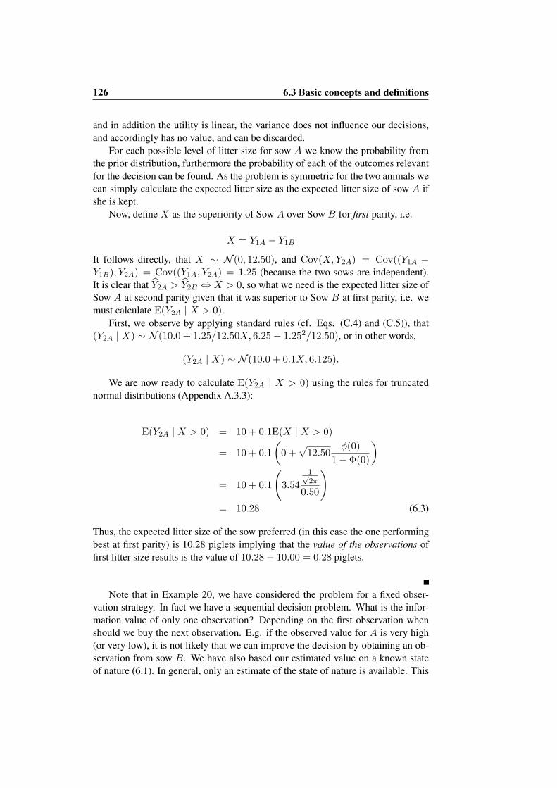
126 6.3 Basic concepts and definitions
and in addition the utility is linear, the variance does not influence our decisions,and accordingly has no value, and can be discarded.
For each possible level of litter size for sow A we know the probability fromthe prior distribution, furthermore the probability of each of the outcomes relevantfor the decision can be found. As the problem is symmetric for the two animals wecan simply calculate the expected litter size as the expected litter size of sow A ifshe is kept.
Now, define X as the superiority of Sow A over Sow B for first parity, i.e.
X = Y1A − Y1B
It follows directly, that X ∼ N (0, 12.50), and Cov(X,Y2A) = Cov((Y1A −Y1B), Y2A) = Cov((Y1A, Y2A) = 1.25 (because the two sows are independent).It is clear that Y2A > Y2B ⇔ X > 0, so what we need is the expected litter size ofSow A at second parity given that it was superior to Sow B at first parity, i.e. wemust calculate E(Y2A | X > 0).
First, we observe by applying standard rules (cf. Eqs. (C.4) and (C.5)), that(Y2A | X) ∼ N (10.0 + 1.25/12.50X, 6.25− 1.252/12.50), or in other words,
(Y2A | X) ∼ N (10.0 + 0.1X, 6.125).
We are now ready to calculate E(Y2A | X > 0) using the rules for truncatednormal distributions (Appendix A.3.3):
E(Y2A | X > 0) = 10 + 0.1E(X | X > 0)
= 10 + 0.1(
0 +√
12.50φ(0)
1− Φ(0)
)= 10 + 0.1
(3.54
1√2π
0.50
)= 10.28. (6.3)
Thus, the expected litter size of the sow preferred (in this case the one performingbest at first parity) is 10.28 piglets implying that the value of the observations offirst litter size results is the value of 10.28− 10.00 = 0.28 piglets.
Note that in Example 20, we have considered the problem for a fixed obser-vation strategy. In fact we have a sequential decision problem. What is the infor-mation value of only one observation? Depending on the first observation whenshould we buy the next observation. E.g. if the observed value for A is very high(or very low), it is not likely that we can improve the decision by obtaining an ob-servation from sow B. We have also based our estimated value on a known stateof nature (6.1). In general, only an estimate of the state of nature is available. This

6.4 Measurement errors 127
will reduce the precision in the information and reduce the value of the information,i.e. it is actually lower than the 0.28 specified.
Naturally utility evaluation of registrations is a very time-consuming task and isusually not possible directly. In section 6.6 this approach towards utility evaluationwill be used on more relevant examples. Now we will continue with other measuresof value and with some attributes of registrations that allows us to evaluate theregistration without considering the decisions involved
6.3.2 Entropy based value
If we wish to record a variable it seems reasonable to select the variable that willreduce the uncertainty most.
A measure of the uncertainty that is often used, is Shannon’s entropy or infor-mation value, as it is also called. The entropy has important applications within theareas optimal coding etc. For instance, the many “zip”, “pack” procedures originatewith this concept. For a discrete variable taking values in the set S = a1, . . . akthe entropy is simply
ent = −k∑
i=1
pilog2(pi) (6.4)
where pi is the probability of observing the value ai ∈ S. (The use of log2 is notessential, but it is the generally accepted logarithm function to use, because in thatcase ent becomes the number of yes/no questions needed to find the value of thevariable.) The formula can be extended to continuous variables. Applying (6.4) tothe sow problem of Example 20 for litter size in first litter (with S = 1, . . . 19)is 3.37, while if the litter size was randomly distributed over the set, S, the entropywould have been 4.25
For a further discussion on myopic (nearsighted) measures of value of infor-mation see Jensen (1996).
6.4 Measurement errors
Another set of attributes of registration concerns the measurement error. In thefollowing different types of measurement errors are discussed.
6.4.1 Registration failure
The first type of the error that can happen in the measurement process is registrationfailure. Registration failure refers to the situation where a registration has gonetotally wrong, e.g. because the record is associated with a wrong identification,a measurement device is read incorrectly, or a wrong number is typed into thedatabase. Such a registration is also called an outlier. Errors of this kind influencethe correctness of a key figure based on the registrations as defined in Section 5.2.4.

128 6.4 Measurement errors
Very often error detection procedures as described in Section 5.2.4 will detectoutliers that are very far from the expected value, while plausible errors will passundetected. A natural model of the outlier is that it is uniformly distributed onthe interval ]µ − κ, µ + κ[ where µ is the expected level and κ is the limit of theerror detection procedure, e.g. κ = 1.96 units of standard deviation. In somedata filtering methods (e.g. Thysen, 1993a) this outlier detection can be handledautomatically, if an estimate of the general error rate, pe, is available, i.e. that weknow how often such an error can occur.
The process of securing that a registration has not failed is some times calledverification of the measurement.
6.4.2 Measurement precision
The simplest error type that can occur is a random difference between the realvalue, X , and the observed, Y . The magnitude of this error is quantified by theprecision using the model,
Y = X + ε (6.5)
where ε is a random and independent error with expectation 0, often it is relevantto assume ε ∼ N (0, σ2
ε) = N (0, 1/τε), where τε is defined as the precision, i.e.,τε = 1/σ2
ε . We will use this definition of the term precision, even for variablesthat are not normal distributed. A measurement error of this kind influences theprecision of a key figure as defined in Section 5.2.4.
If we take the average of k independent measurements, the precision of theaverage is kτ . Note that the independency between measurement is important, ifthe relation is to hold.
Some times the term repeatability, t, is used for measuring the quality of aregistration. Repeatability is most often defined as the correlation between twomeasurements on the same subject, i.e., in this case:
t =Cov(Yi, Yj)
Var(Yi)=
Var(X)Var(X) + σ2
ε
(6.6)
When the precision increases, the repeatability approaches one. Note, however thatthe variance of the subjects measured will have a large impact on the repeatabilityof the measurements, while the precision is not influenced.
6.4.3 Indirect measure
Often the measurement taken is only an indirect measure of the true value. Mostmeasurements are in fact indirect, such as hormone analysis etc. Measurementerrors of this type influence the validity of a key figure as defined in Section 5.2.4.The value that we want to measure may even be some abstract phenomenon.
A simple case is the trait that we measure is not constant but varies aroundsome value

6.4 Measurement errors 129
Y = X0 + εx + ε.
Here we have introduced an additional error term. We still have our “old” mea-surement error but in addition we have an error term that represents how goodour indirect measure is. If εx has a low variance, the two variables will be highlycorrelated and we can obtain a good measure of the underlying trait. Repeatedmeasurements will not generally solve the problem of low precision. Repeatedmeasures improve our precision in X0 + εx. A good example is pregnancy testingusing ultra sound. Some times the pregnancy tester will react to something differ-ent than a pregnant uterus. If we repeat the testing, we will repeat the failure. Only,if the measurements are independent both with respect to εx and ε can we improvethe precision by repeated measurement.
This case of indirect measure is in general too simple. Instead, if X is what wewant to know, but Y is what we measure, a more general model would be,
Y = f(X) + ε
Y ≈ X0 + β1(X −X0) +12β2(X −X0)2 + ε,
where the approximation is based on a second order Taylor series. If the measure-ment is properly calibrated and developed, the relation will be very close to linearand the second order term will vanish. On average the measurement would givethe correct result and we can treat the deviation as random. If this is not the casewe get a systematic difference in level, and our measurements becomes biased.
The validity concept is also sometimes used for single measurements (i.e. notjust for key figures as in Section 5.2.4), i.e. if Var(εx) is low the validity of themeasurement is high.
6.4.4 Bias
The concept of bias may be represented as ι in
Y = X + ι+ ε
Bias should always be treated with caution. Usually we tend to think that if wemeasure more individuals we get a more precise estimate. This is only the case ifthe measurements are unbiased. If the bias is known, we can of course correct forit, and then we have by definition removed it.
A good example of bias is the use of perching equipment with weighing sen-sors. In the start of the growing period every animal uses the perch with equalprobability, but when the animals become older, the heaviest animals have a lowerprobability of resting on the perch. The resulting weight measurement is thus sys-tematically underestimated, i.e. they are biased.

130 6.4 Measurement errors
6.4.5 Rounding errors
When results from measurement devices are read, the figures are usually roundedto some extent. A systematic rounding method implies that instead of using themeasurement, XO, directly we can assign an interval to the measurement i.e.,X ∈]XO − 0.5, XO + 0.5]. Very often, however, the rounding is not system-atic. It is much more tempting to round off from 9.41 to 9.4 than from 9.4491 to9.4. Very often the last figure would be registered as 9.45, although most of theother registered values are with only one digit after the decimal point. However,in animal production this is not likely to cause any major problems, because of themuch more serious sources of errors.
6.4.6 Interval censoring
The rounding errors can be generalized to the concept of interval censoring, i.e.where only some threshold values τ0, τ1, τ2, . . . , τn are registered. For examplemating and farrowing, are usually registered on a date level, so that we only knowthat the measurements are between two of the threshold values.
When the underlying distribution is continuous we can still model the data,based on the probability that the observed value is between the two thresholds.
Example 21 Pregnancy period in sowsThe interval from mating to farrowing in sows is approximately distributed asN (115, 2.52). If a sow farrows on day 116 we can calculate the likelihood of thisobservation as Φ(117, 115, 2.5) − Φ(116, 115, 2.5), where Φ(x, µ, σ) is the prob-ability of value less than x from a normal distribution with mean µ and standarddeviation σ.
Note that the censoring can also occur with the threshold values of ±∞, i.e. ifan event occurs, it is before or after the specified registration time. Typical exam-ples are when registrations are started in a herd and the previous history is unknownor when data has not yet been registered. An example of the latter case, is whenfarrowing/calving rates are to be calculated, based on observed matings before thebirth takes place. For some of the animals a new event has been registered (remat-ing), while for others no remating has taken place.
6.4.7 Categorical measurements
The concepts used for interval censoring can be further developed to cover thecategorical or qualitative measurements, such as heat detection in oestrus, not inoestrus, pregnancy diagnosis pregnant, not pregnant, disease diagnosis dis-eased, not diseased, leg weakness score etc. In contrast to the interval censoringcase, the registrations are not the threshold values, but rather the number of theinterval. i.e. the state of the animal can be d1, d2, . . . , dn.
The measurement w can be thought as a two-step procedure.

6.4 Measurement errors 131
Table 6.1: The outcomes from oestrus detection of sows. Sensitivity and specificityof the measurement.
Actual StateDiagnosis Not in oestrus In oestrusNegative 0.99 0.05Positive 0.01 0.95
Table 6.2: The outcomes from pregnancy diagnosis of sows. Sensitivity and speci-ficity of the measurement.
Actual StateDiagnosis Not pregnant pregnantNegative 0.70 0.05Positive 0.30 0.95
1. Measurement of a continuous variable yw, where yw is distributed asN (µi, σ2w)
if the animal is in state i, and the measurement precision is 1/σ2w.
2. Assignment of a state dj to the measurement depending on a series of thresh-old values τ0, τ1, τ2, . . . , τm, where m normally (but not necessarily) isequal to n−1. The threshold values are specific for the measurement method,such that the animal is said to be in state di if τi−1 < yw ≤ τi (τ0 is definedas −∞).
The concepts are further illustrated through Example 22.
Example 22 Heat detection and pregnancy test in sows.Heat detection (oestrus detection) in sows typically has a low error rate and thevalues shown in Table 6.1 are fairly representative.
This can be modeled as an expected value of 0 for sows not in heat and 1 forsows in heat, σw is 0.252 and the threshold value 0.5858. The distributions areshown in Figure 6.1.
Pregnancy testing can be done with an automatic testing device with a relativelylow detection precision. A typical example is shown in Table 6.2.
This can be modeled as an expected value of 0 for sows not pregnant and 1for pregnant sows, σw is 0.4610 and the threshold value 0.2417. As shown inFigure 6.2 the two distributions have a considerable overlap. Note that the standarddeviation on the underlying scale is almost twice as big for pregnancy diagnosis,as for heat detection.
The elements of Table 6.2 are often called sensitivity and specificity with termsborrowed from laboratory measurements. In this context the sensitivity is the prob-ability of detecting a phenomenon, when it exists, i.e. in the case of pregnancydiagnosis 0.95. The specificity is one minus the probability of observing a phe-nomenon, when it is not there, i.e., 0.7.

132 6.4 Measurement errors
-1 0 1 20
0.5
1
1.5
Underlying value
Density
Not in Heat
In Heat
Threshold
Figure 6.1: Threshold model for heat detection
-1 0 1 20
0.5
1
1.5
Underlying continous value
Density
Not pregnant
Pregnant
Threshold
Figure 6.2: Threshold model for pregnancy testing

6.4 Measurement errors 133
P(-|-)
0.40 0.50 0.60 0.70 0.80 0.90 1.00
0.40
0.60
0.80
1.00
P(+|+)
Heatdetection
Pregnancydetection
Figure 6.3: Possibilities for calibrating heat and pregnancy detection
Another, concept is the predictive value, i.e., the probability that an animal thatis diagnosed as pregnant, really is pregnant, and vice versa. This is the value thatis most import in a decision context, but it depends on herd level of pregnancy rateas well as the measurement device. Using Bayes rule (Theorem 1), the differentvalues can be calculated.
In a typical measurement apparatus the threshold value can be altered, andthe variable measured will be continuous. This very closely resembles our model.Correspondingly, the threshold can be altered to give a large spectrum of detectionrates. In Figure 6.3 this is shown for the two measurements discussed. The optimalcalibration will depend on the proportion of positive and negative animals in thepopulation as well as the decisions taken after the measurements have been made.It is questionable if a general calibration is optimal. The calibration should betuned to the herd that is using the device.
6.4.8 Enhanced models of categorical measurements
The models above are too simple to be of value in the evaluation of measurementmethod. It is assumed that repeated observations are independent. Observationson the same animal within a short time period will usually tend to give the same

134 6.4 Measurement errors
result. The trick is to model the repeated measurement on the continuous scale asdiscussed above and then to proceed with the classification later on based on thethreshold values.
Let Yit be the value measured for animal i at time t. A more detailed modelthat can account for repeated measurements is
Yi,t+∆ = f(t+ ∆) +Ai +Mi,t+∆ + εit, (6.7)
where ∆ is a small time interval, f(t) is a function representing the effect of the truestate of the animal at time t, e.g. pregnant versus not pregnant, Ai ∼ N (0, σ2
A)is a random effect of animal, Mit is an observation from an autocorrelated timeseries, and ε is the random measurement error. The autocorrelated time series mayfor instance be modeled as
Mi,t+∆ = exp(−α∆)Mit + εM , (6.8)
where α is a parameter measuring the size of the autocorrelation, and εM ∼N (0, σ2
M ). With this model, measurements with short intervals will be close invalues (high repeatability) and measurement far apart will be less correlated
The A and M parameters may have to be modeled separately for each of theunderlying states (e.g. one set of models for pregnant and an other set for notpregnant).
6.4.9 Pre selection
Many registrations are performed on a selected material. An example is weigh-ing of slaughter pigs. Before delivery to the slaughterhouse a visual inspection isperformed, and the candidates for delivery are weighed.
In other words, the measurement is a two-step procedure. First a measurementZi (visual inspection) is made on every individual in the pen. The measurementsare ordered according to size, and the first in the list is weighed on a scale, i.e. theobserved value is:
Yi = (Xi|max(Z1, . . . , Zn) = Zi)
where Xi is the true live weight and Yi is the observed live weight. Clearly weshould take care, if we use Yi as a representative measurement of the live weightof the pigs in the herd.
6.4.10 Registration of interventions
Intervention occurs when the manager believes there is a problem that he can re-move by some kind of action. Treatment of disease is an example. Note that thisregistration is no indication of the problem. It is a combination of the farmer’s sen-sitivity as well as his trust in the action. Symptoms can be registered objectively,

6.4 Measurement errors 135
not the diagnosis. Culling reasons is an example of how the registration system al-most forces the farmer to diagnose a disease when he culls rather than objectivelyreport symptoms.
6.4.11 Missing registrations
The intervention registration has a parallel in the concept of missing registrations.In fact if we know the behavior of the manager, there is information in the regis-tered value as well as the values not registered.
For example, we would expect a mated sow with no further registration the last80 days, to have a high probability of farrowing. If it had shown oestrus we wouldhave expected it to have been registered, either as a remating or as a culling. Lateron, if there is no farrowing past 118 days after mating, we would suspect that shehas not been pregnant, even though there is still a small probability that she willfarrow.
6.4.12 Selection and censoring
Some of the most difficult measurement errors are the errors that occur because ofwhat we can call selection within the data, or censoring of observations.
Again the problem is that the farm is under strict management control, andthat the traditional assumptions of independency and randomness of observationstherefore cannot be justified.
Cows with a high milk production will tend to have longer lactations as wellas a higher longevity. Sows with high litter size will have higher longevity. Fastgrowing slaughter pigs, will be delivered before the slow growing.
If the manager would maintain the same control of the herd, this was not aproblem, because eg. the expected lactation yield in late lactation in old cowswould be the same as that previously recorded. But if he changes strategy, andreduce e.g. the culling rate the old value will not be correct anymore, becausesome of the low producing cows will reach the high age.
Therefore the data should be processed using methods that can take the selec-tion into account.
Example 23 Daily gain in slaughter pigsTo illustrate the problem of censoring in practice, the problem of the calculatingaverage daily gain will be discussed. Most slaughter pig units use a managementinformation system reporting the so-called average daily gain in the herd. It mayfor instance be calculated straightforward as
DGH =
∑ki=1
1ksSLWi −
∑ki=1W0i∑k
i=1 tsi − t0i
where ks is a constant for the slaughter waste, SLWi is the slaughter (carcass)weight of the ith individual,W0i is the weight at the start of the fattening period, tsi

136 6.4 Measurement errors
is the time at slaughter of pig i and t0i is the time at insertion of the pig. The reasonfor this formula is that a linear growth is assumed, and under that assumption weobtain the following formula:
DGH =∑k
i=1(W0i +DGi(tsi − t0i)−∑k
i=1W0i∑ki=1 tsi − t0i
=∑k
i=1DGi (tsi − t0i)∑ki=1 tsi − t0i
(6.9)This definition would have been correct if the animals were delivered at the sameage. Assuming fixed age at insertion, delivery at the same age implies that, ∀i :tsi − t0i = c. By insertion in (6.9) we get,
DGH =∑k
i=1DGic∑ki=1 c
=c∑k
i=1DGi
kc=∑k
i=1DGi
k.
Then, average daily gain for the herd is the average of the individual daily gains.Unfortunately, pigs are not delivered at the same age. Instead, they are deliv-
ered at a constant weight, i.e. we have that DGi(tsi− t0i) = K. This is a standardexample of selection or informative censoring. If we substitute this into (6.9), weobtain
DGH =∑k
i=1K∑ki=1
KDGi
=k∑k
i=11
DGi
i.e., the daily gain observed in the herd is the harmonic mean of the daily gainsof the individual pigs. Compared to the usual arithmetic mean the harmonic meanplaces more emphasis on the low value. The slowest growing pigs influence themean more than the fastest growing. They spent more time in the herd, so in thatrespect, it is reasonable enough.
In fact not every pig is delivered at a constant weight. Before a pen becomesavailable to new pigs it has to be emptied. Therefore economic considerationsmean that some of the pigs are delivered at a lower weight. If the slaughter pigmanager uses sectioned production this has even higher effect, because the slowgrowing pigs occupy a whole section, i.e. more pigs should be delivered at a lowweight. An indirect result of this is that sectioned production will have a higherdaily gain, because the formula for calculating herd daily gain is more like an arith-metic average, than in normal continuous production, where it closely correspondsto the harmonic mean.
Usually the selection bias in sows or dairy cows will be in the opposite directionof what is seen in Example 23, i.e. the best animals would tend to be longer in theherd, and thus have a higher impact on the herd level.
We would usually think that this would lead to an overestimate of the produc-tion curve, but it may in fact draw in the opposite direction if statistical proceduresare not used correctly. A typical statistical model for repeated measurements is
Yit = µt +Ai + εit

6.5 Data processing 137
Using standard methods such as the GLM procedure (SAS Institute Inc., 1989) wewould declare the animal effect as random with mean 0, and variance σ2
A. If onlythe best animals remain in the herd, the average at high parities of the A-valueswould be higher than 0. In order to compensate for this, the statistical methodwould reduce µt correspondingly. Toft and Jørgensen (2002) describe a maximumlikelihood based method for unbiased estimation of the litter size curve in sows.
6.4.13 Discussion
The list of possible measurement errors has become rather long, in fact so longthat it seems like a specification of Murphy’s law within measurement in animalproduction herds (If anything can go wrong, it will). The important message isthat if we can identify and describe the error source and type, there will often bestatistical methods available that can handle that error, and make correct deductionsfrom the registration possible, despite the errors. If the errors are not detected,faulty conclusions will be the result.
6.5 Data processing
Methods for data processing is outside the scope of this note. Instead the dataprocessing will be classified according to the herd management cycle, and generalattributes of the data processing discussed.
If we compare Figure 1.1 with the examples in Section 6.2, we find that almostall of the examples have to do with either the implementation or the monitoringphase of the management cycle, and that the use in the implementation phase hasto do with operational decisions that very closely resemble the monitoring process.The data are collected in order to detect deviation from a level previously defined.When this deviation is detected, an action is taken. The heat detection problem isthe implementation phase, a detection of oestrus signs above a certain thresholdresults in a mating. The weighing problem is either operational, i.e. if the weightis above a threshold deliver the animal, or monitoring, i.e. if the average growthrate is below some limit, start an analysis. The climate regulation based on activ-ity is clearly in the implementation phase where in fact the actions based on themeasurements is effected wholly automatic, without the intervention of a humandecision maker.
For monitoring and operational purposes the data processing leads to very sim-ple information, because the information is only used for selecting between twoactions, i.e Ignore evidence, React to evidence.
Strangely, the use of data for planning purposes is largely overlooked, when thepossibilities for new registrations are discussed. Of those examples mentioned insection 6.2, only the detection of position of free ranging animals is actually a plan-ning parameter. If we know where the animals are, we can plan inspection visitsetc. But this can easily be implemented on the smaller scale in a herd. Monitoring

138 6.5 Data processing
the number of animals in the herd and their growth rate gives a precise prognosisof future productivity, and the best possibility for management of feed inventory,manure, new animals etc. The different approaches to decision support presentedin Chapter 9 all rely on a knowledge of the state of nature in the herd, i.e. a compli-cated processing of data from the herd. It is of interest to note that the informationfrom the data processing is used for much more complex decisions, i.e. the futureproduction plan. Clearly the impact of the correct information becomes larger.
The optimal statistical methods for data processing are to be found within theanalysis of time series and longitudinal data, even though the papers presenting theapplication of the measuring methods in general rely on a more ad hoc solution tothe data processing. This adaptation of statistical methods to the specific problemsin herd management will be an important research area in the future.
6.5.1 Threshold level
The direct detection of a measurement above a threshold level is in fact directlycomparable with the model of quantitative measurement presented in the previoussection. With a given measurement precision we can calibrate the threshold toobtain different levels of sensitivity and specificity of the test. If we measure theweight of an animal in order to decide whether to deliver it to the slaughter house,we can set the weight threshold high and then secure that a very low percentageof the animals are delivered too early (with too low a carcass weight), i.e. a highspecificity. In doing this, many animals that are actual in the correct weight groupwill not be delivered, i.e. the sensitivity of the test is too low. The choice ofthreshold weight will of course depend on the distribution of carcass weight withdifferent threshold weights and thus the economic income.
The measurements are very often repeated, and apart from sensitivity and speci-ficity the detection time becomes an important attribute of measurements in dy-namic systems. When the repeated measurements are independent, the sensitivityof the measurement will increase, because the probability of a value above thethreshold will increase with the number of repeated measurements. For exactly thesame reason the specificity will decrease. In addition, we have to consider the timeof detection as well. For example in oestrus detection, it is not very interesting toregister the oestrus if the registration is too late to result in a fertile mating.
Usually sensitivity and specificity of threshold level detections should be spec-ified per time unit. For example in oestrus detection, percentage detected the first12 hour of oestrus, or with threshold detection for control purposes, number offalse alarms per year.
Measurements that can rely on a threshold level do not need a very high detailin registration identification. I.e. we do not need the identification of the individualanimal. This can result in large differences in the cost of an automatic system.

6.5 Data processing 139
6.5.2 Change point estimation
Very often the purpose of a measurement is not to detect a value above a certainlevel but to investigate a change in level. In the statistical literature this is calledchange point estimation. This comprises detection of sudden changes in the levelof a variable as well as changes in trend.
The method of change point detection is often suggested, when the thresholdlevel mentioned above fails, i.e. in heat detection based on temperature measure-ments, it is suggested to correct for the level of the individual sow. From a concep-tual point of view a change-point detection is simply the detection of a change withmagnitude above a certain threshold level, and the method is thus very comparableto the method above.
There are important differences, however.
• The change-point estimation needs data-processing, i.e. data should be inputand processed in some kind of computing facility before it can be reactedupon.
• The change-point estimation needs identification. When comparing the lev-els at different measurements, it is necessary to identify each registrationitem (e.g. animal) and connect the data items. Often this requires a com-pletely different setup, i.e. for automatic registration use of an automaticidentification equipment. In addition it can result in a new set of measure-ment errors, i.e. we need to consider the possibility for mis-specification ofidentification and the errors this can cause.
• The change-point estimation is less precise. The variance of the differencebetween two independent and identically distributed variables is twice thevariance of each of the variables.
• The change-point detection needs more registrations and the detection willbe later than with the threshold value.
A thorough investigation is needed, before it can be concluded that the change-point method will be able to solve problems that the simple threshold techniquecannot solve. This consideration should also include the timeliness of the detection.For control purposes it is relevant to ask, how a detection of a change point half ayear ago can improve the future production in the herd.
At the herd-level change-point methods are important for planning purposes.Even if there is only a weak evidence for a change in the level, it is important totake this evidence into account when making plans for the future.
6.5.3 Significance test in experiments
This final method is only to illustrate the similarity between the decision supportfor experimental purposes and for herd management purposes.

140 6.6 Utility evaluation examples
The traditional statistical method for experimental design and analysis is ofcourse a processing of data, and it corresponds very closely to the qualitative mea-surement problem, with sensitivity and specificity. Even though, many data areregistered in the experiment, the information from the experiment after processingshall be used to select between two actions (Reject Null-hypothesis, Do not rejectNull-Hypothesis). Because it is generally impossible to assign utilities to these al-ternatives, the selection of threshold value is based on a fixed and widely acceptedspecificity of the experiment, i.e. the so-called type I error, or the significance level(e.g. 5%). If the null hypothesis is true, there is only a low risk of rejecting thenull-hypothesis. As the null hypothesis corresponds to the old scientific theory, itis natural for the research community to be conservative in rejection the hypoth-esis. The statistical procedures modify the threshold value to keep the specificityconstant.
The sensitivity of the experiment is controlled by the individual researcher, theso-called type II error, mainly by making the experiment as precise as possibleunder the economic constraints. An accepted choice is a type II error of 80%.Clearly, the cost of failing to reject the null hypothesis (i.e. document a new the-ory) is mainly with the individual experimenter, and he/she must evaluate the costshimself.
In conclusion, the experimental procedure is a method for measurement in or-der to make decisions concerning scientific theories. The value of a correct scien-tific theory is impossible to estimate. Therefore, the threshold value in experimentscannot be set according to utility, but sensitivity and specificity have to be used in-stead.
6.6 Utility evaluation examples
6.6.1 Production control
Production Control in sow units is carried out in order to detect deviations from aplanned level. The decision to be made based on the production control is whetherto continue production according to the original plan or to change production plan.As an example, the Danish Efficiency control has been studied (Jørgensen, 1985).In this control system several traits are registered and presented to the farmers asquarterly averages. These averages fluctuate either due to random influences ordue to systematic deviations from the planned level. By observing the productiontraits during a production period a better knowledge of the expected future levelsis obtained. The deviation of the individual trait from the expected level can beweighed with the marginal value of the trait, and an estimate of the economic valueof the deviation can be obtained. By comparing these deviations to the expectedvalue of an other plan, the decision whether to alter the production in the future canbe made. A similar approach has been used by Huirne (1990).
The improvement in income from these changes in production plan is equal tothe value of the production control. The possible decisions are to continue with

6.6 Utility evaluation examples 141
Marginal value Relative value
Mortality, piglets %Farrowing section, usage %
Litter size, parity >2Litter size, parity 2Litter size, parity 1
Growth rate, weanersPregnancy rate, %
Weaning to cull, daysMatings before 21 days %
Age at selling, weanersWeaning age
Culled after weaning, %Mating to cull, days
Feed pr dead weaner, estWeaning - 1. oestrus, daysCulled after weaning, %
Production traits
Figure 6.4: Value of different traits in production control in sow units
same production plan or to alter the plan. The first two moments of the priordistribution are the expectation and variance for production traits and expectedincome under the other production plans. The first two moments of the posteriordistribution are the conditional expectations and variance given the observed levelof production trait in the control. The loss functions (that are minimized) are minusthe expected income from the current plan and minus the expected income from theother plan with the cost of changing plan included.
In the study by Jørgensen (1985) it was shown that the registrations in the Dan-ish efficiency control could be expressed from 16 major traits. The distribution ofquarterly averages of these traits were approximated with a 16-dimensional normaldistribution. Based on registrations from 100 sow herds in the Danish Applied PigResearch Scheme, ’Den rullende Afprøvning’ (Pedersen et al., 1995), the variancein these traits was divided into variance between herds and variance within herds.From these variance-covariance matrices it was possible to specify the prior andposterior distribution of the traits. The loss functions representing expected in-come in the herd were calculated using standard prices. From these parameters itwas possible to calculate the value of the production control. The study showed anoverall improvement of 6-7 % in total income from using the control. Furthermore,the marginal values of different production traits from a control point of view werecalculated in the study. The sequence of the traits to be included was chosen tomake the highest marginal improvement in value for each new trait.

142 6.6 Utility evaluation examples
As shown in Figure 6.4, the most important traits to monitor are piglet mor-tality; usage of farrowing department; litter size in parity 1, 2, and 3 or higher;growth rate of piglets; and pregnancy rate. It is important to note that the littersize in the different parities treated separately has a value on their own. The rec-ommendations of Sundgren et al. (1979) of treating these traits separately was thusconfirmed in this study. These 7 traits accounted for almost all of the value of thecontrol.
The conclusion on the study was that the use of the efficiency control did in-deed improve the expected income, but this improvement could be obtained fromfewer registrations than currently used. The emphasis should be on controlling thequantitative aspects of the whole herd’s production, instead of a detailed control ofindividual performance.
6.6.2 Recording of sow specific litter size
As mentioned in the previous section, the registration of parity specific litter size inthe herd is one of the most important registrations from a production control pointof view. This might indicate that litter size of the individual sow is an importanttrait. Several authors have investigated the possibility for culling sow with respectto litter size, e.g. Strang and King (1970); Treacy (1987); Huirne et al. (1991).
The decision is relatively straight forward; if the sow obtains a litter size lowerthan a specified norm at a given parity, it should be replaced by a replacement gilt.The improvement in expected income by using information concerning litter sizecould be used, or, as in the following, the improvement in expected average littersize. Jørgensen (1992) considered a modification of the method used by Huirneet al. (1991). From this paper results concerning detail of information will bepresented. Three levels of information were considered. No information, i.e., onlyinvoluntary culling; Parity information, i.e, only the parity of the sow is known;and Litter size, i.e., the litter size in each previous parity of the sow is known. Therelationship between parity and litter size and involuntary culling was assumed tobe known as well as the relationship between litter size in subsequent parities.
In Figure 6.5 the relationship between involuntary culling and average littersize is shown using the three levels of information. The level of involuntary cullingis measured by the average age in the herd, if only involuntary culling was used.The level of in voluntary culling is assumed to be slightly increasing with parity.As can be seen the culling strategy improves the average litter size, at least for thelow level of involuntary culling (i.e., high average age). The difference between thestrategy using sow specific information and the strategy using only parity specificinformation is very low (less than 0.1 pigs per litter).
Furthermore, in Figure 6.6 a more realistic situation is presented, where slightlywrong estimates of the influence of parity on involuntary culling is used whencalculating the culling strategy. The use of these erroneous estimates results in areduction in expected in litter size, compared to the situation where no ’Optimal’

6.6 Utility evaluation examples 143
3 4 5 6 7 8 910
10.5
11
11.5
No culling Parity Sow
Average parity without voluntary culling
Litter size, avg.
Figure 6.5: Value of different traits in production control in sow units
0 2 4 6 8 10-0.2
-0.1
0.0
0.1
0.2
0.3
0.4
0.5
0.6
Average parity without voluntary culling
Improvement in litter size
constant involuntary culling
age dependent invol. culling
Optimal culling
Estimated age
used in
optimization
Figure 6.6: Effect of using wrong parameters when calculating ’optimal’ strategies

144 6.6 Utility evaluation examples
culling strategy is used. The magnitude, 0.1 pigs per litter, is fully comparable tothe maximum possible benefit of using the culling strategies.
As a conclusion, due to the low value of sow specific information, decisionsupport models for sow culling do not necessarily need to include the variancebetween sows with respect to litter size. This gives a considerable reduction innecessary calculations and complexity of the model used. However, the problemis to estimate the influence of parity on the relevant traits in each herd. As thiswould have to be done on selected data, it is no trivial task. A method for this hasbeen described by Toft and Jørgensen (2002), and later Kristensen and Søllested(2004a,b) have developed a sow replacement model based on parameters estimatedfrom herd specific data using the method of Toft and Jørgensen (2002).
6.6.3 Precision in weighing of slaughter pigs
Weighing of slaughter pigs is often considered necessary in order to obtain effi-cient production. From a decision point of view, weighing can be used as a controlof growth, and for deciding, when to deliver the slaughter pig to the slaughterhouse. Jørgensen (1993) studied the problem in detail and the following is an ex-tract of that paper, analyzing the use of weighing when selecting pigs for slaughter.Several methods for weighing or estimation of live weight have been suggested:the traditional individual weighing; electronic weighing equipment with electronicidentification of the individual pig; weight assessment using the dimensions of thepigs, e.g., through image analysis; and, finally, simple visual assessment of weight.These methods will be expected to differ in precision, or to put it in another termto have different variance. As the cost of weighing differs markedly, an estimate ofthe value of an increase in this precision would be of interest.
In Denmark slaughter pigs are priced according to their slaughtered weight, andfurthermore graded according to meat percentage. Pigs with a slaughter weight inthe interval between 70-85 kg will obtain the highest price per kg. Thus, there isan incentive to deliver pigs with the right slaughter weight. A pig producer canonly measure the live weight of the pig, and has to decide, whether to deliver ornot, based on this criteria. He will necessarily have to cope with a variation aroundthe desired slaughter weight. Furthermore, he has to report how many pigs he willdeliver to the slaughter house approximately 3 days in advance. Usually he canonly deliver pigs once or twice a week. The pig producer uses the decision rulethat if observed live weight of the pig is larger than a threshold weight, the pig isdelivered three days afterwards1. If not, the pig is kept in the herd until the nextweighing a week afterwards. However, if the expected return in the next week islower than the expected return of a new pig, the pig is also delivered, regardless ofweight. After delivery the pig is replaced with a new pig after a week for clean-ing of the pen. A probabilistic simulation model (Jørgensen, 1991) was used in
1It is realized that this decision rule is not optimal, a kind of regression equation would improvethe decisions. However, this decision rule, is the rule generally recommended by advisers

6.6 Utility evaluation examples 145
0 0.2 0.4 0.6 0.8 16450
6500
6550
6600
6650
Weighing precision, 1/kg
Future value, DKR
Weighing No weighing
Image analysis
Visual
Traditional
Automatic
Figure 6.7: Influence of weighing precision
order to calculate proportion delivered on each day after insertion, and correspond-ing expectation and variance-covariance matrices for total feed consumption andslaughter weight. Assumptions of multivariate normal distribution is used. Theexpected future value (FV) of the production using an interest rate of 0.1 is calcu-lated for each threshold live weight and the optimal threshold live weight is found.Prices and costs correspond to the level in Denmark in the middle of December1991. In Figure 6.7 the future value is shown, for different values of the weighingprecision, (1 divided with the standard deviation).
The markers in the figure correspond to preliminary estimates from a studyat our institute. With a weighing precision of 1 the value of the weighing is 150DKK in FV compared to a fixed delivery date, or approximately 4 DKK per pigproduced. Compared to simple visual estimation of weight the value of weighingis approx. 2 DKK.
It must therefore be concluded that with the current pricing system there isnot much economic value of weighing. Automatic weighing equipment in com-bination with electronic identification cannot even earn the cost for the electronicidentification tag. The value of weighing might, however, be found in other pro-duction phases, e.g., in growth and feed control and estimation of growth and feedconsumption curves for the individual herd.
146 6.7 Outlook
6.7 Outlook
As shown it is possible to get indications of the value of registrations from a de-tailed analysis of the decision process, and the related stochastic variation in stateof nature. The registrations used in their traditional context have shown only aslight improvement in expected utility, or as in the case with the pregnancy tester,even a negative effect. On the other hand, if the registrations are used in a differentdecision context, they can have positive influence. The estimation of utility valueoften indicates these other uses of registration.
The notion of negative value of information is important. Researchers trying todevelop decision support systems should have this in mind. Also the value of thesystem should be compared to systems with a lower need for information. Usu-ally it is assumed, that the prior distribution of the traits is known. We usuallyassume that we know how litter size depends on parity, we know the relationshipbetween growth rate, feed consumption and age, etc. This knowledge is, however,based on experimental results or from other production herds, and might not berelevant for every herd. In practice, the most important problem seems to be howto obtain herd specific estimates of these relationships. If we are not to overtax theanimal producers with information from the profusion of possible registrations, weneed to identify the decisions made in the herd. Then we should consider, whichinformation is used in the decision.
Finally, we should investigate, whether some relevant data is missing, andwhether the data can be obtained in a cost effective way. Then we might suggest tothe animal producers, that they begin to use these data.

Chapter 7
Dynamic production monitoringby classical methods
Automatic monitoring of animal production is not very common compared to whatis usual in industrial production, where key variables are registered and analyzedstatistically during the entire production process in order to quickly alarm aboutany deviations from the norms.
In animal production current standards for monitoring are as described in Chap-ter 5. Thus, quarterly or monthly reports with selected key figures is the mostcommon form of monitoring.
In order to improve the production process, a more dynamic monitoring methodis desirable. Collecting data (and in what way) has been covered in Chapter 6. Itis now time to look at the use of data for monitoring the production process in adynamic way. Statistics provides us with an analytical framework to handle theuncertainties inherent in especially animal production. This also means that thetopics covered here will become more mathematical in nature.
The main problem with the current chapter is, however, that it has not yet beenwritten. Instead, readers are encouraged to consult an excellent book by Mont-gomery (2005), where in particular Sections 4.1 - 4.3.5, 5.2.4, 8.2, 8.3, 9.4-9.4.2are recommended. Those sections cover
• Sheward control charts.
• Moving average control charts.
• Exponentially Weighted Moving Average (EWMA) control charts.
These straight forward monitoring methods have only been applied very littleto animal production. A few examples in dairy cows, nevertheless, include Thysenet al. (1988); Thysen (1993b) (in particular the EWMA method is applied). Morerecent examples are de Vries (2001); de Vries and Conlin (2003, 2005).

148

Chapter 8
Dynamic production monitoringby state space models
This chapter continues the efforts for creating a consistent framework for dynamicproduction monitoring. From the herd manager’s point of view, animal productionis a sequence of decisions based on a continual stream of information. Hence, thereis a need for a framework which allows knowledge to accumulate, so that it may,in principle lead to improved understanding of the production and, in consequence,better decisions. Dynamic linear models (DLM) are a possible approach to providesuch a framework in which relevant prior knowledge and current information iscombined into a coherent tool for decision making. Those models will be thecornerstone of this chapter.
Again, however, the main problem with the current chapter is, that it has notyet been written. Instead, readers are encouraged to consult a paper by Thysen(1993a) presenting the simple dynamic linear model and the multiprocess model.It is a much more accessible text than the textbooks mentioned below, but it is nota proper substitution.
The best textbook on Dynamic Linear Models is in our opinion still West andHarrison (1997). A more accessible textbook is Poole et al. (1994).
Three papers by Madsen and coauthors (Madsen and Ruby, 2005; Madsenet al., 2005; Madsen and Kristensen, 2005) are examples of applications with pigproduction.

150

Chapter 9
Decisions and strategies: Asurvey of methods
9.1 Framework of the survey
In Chapter 1 we defined (Definition 2) the information needs for decision makingto include
1. The current state of the unit.
2. A production function describing the immediate production given stage, stateand decision and the distribution of the possible random term(s).
3. The distribution of the future state given stage, state and decision.
4. All attribute functions relevant to the farmer’s preferences.
5. The utility function representing farmer’s preferences.
6. All constraints of legal, economic, physical or personal kind.
The purpose of this chapter is to provide a general overview of techniquesavailable in the determination of optimal decisions and strategies.
The techniques will be described according to their ability to represent thevarious kinds of necessary information listed above. Furthermore, their potentialsfor integration of decisions at different levels and time horizons defined in Chapter1 are discussed. It is not the purpose to describe the various methods in details,but only to provide a general survey relating to the issues of the previous chapters.Details about the methods are left for separate chapters.
9.2 Rule based expert systems
Research concerning expert systems is a development within the area called Artifi-cial Intelligence (AI). The British Computer Society has defined expert systems as
152 9.2 Rule based expert systems
follows (cited from Dindorph, 1992): An expert system is regarded as the embod-iment within a computer of a knowledge-based component from an expert skill insuch a form that the system can offer intelligent advice or take intelligent decisionabout a processing function. A desirable additional characteristic, which manywould consider fundamental, is the capability of the system, on demand to justifyits own line of reasoning in a manner directly intelligible to the enquirer. The styleadopted to attain these characteristics is rule-based programming. This is just oneof many proposed definitions of expert systems.
The fundamental difference between the rule based systems, and the approachthat we have presented until now, is that instead of trying to model a system, therule based expert systems tries to model the expert, or rather the expert’s approachto problem solving. Originally, the ambition within AI-research was to make gen-eral problem solvers that could be used for any problem area, but this was realizedby most researchers within the area to be overambitious. The research efforts had,however, led to new approaches towards problem solving, and within narrow prob-lem (expert) domains, the approach showed some promising results.
Rule based expert systems have three components: a knowledge base contain-ing the expert’s knowledge of the domain, an inference engine that decides howand when to use the knowledge, and a user interface.
The knowledge base contains knowledge of a problem domain, as it is de-scribed in text books, as well as expert knowledge, e.g. exceptions to generalrules, experiences from previous problems, and time-efficient approaches on howto solve problems within the area. The knowledge base is an enhanced data basethat apart from data also contains logic rules for the connection between the itemsin the knowledge base, e.g if x or y then z.
The inference machine contains the mechanism for deduction based on thelogical rules in the knowledge base. The deduction can use different inferenceprinciples, such as backward chaining and forward chaining. In the rule showedabove, the inference machine would start out by finding the value of z, and giventhe knowledge of z establish the value of x and y. Forward chaining would startout by establishing the values of x and y and deduce the value of z subsequently.In both cases the unknown values are found either by a question to the user orby combining other rules in the knowledge-base. The optimal choice of inferenceprinciple depends on the type of problem the expert system is supposed to solve.In very complex expert systems, neither forward nor backward chaining is fastenough, and the so-called heuristic search strategies are needed. These strategieswork primarily by searching the knowledge base in an efficient order, focusing onareas, where a solution to the problem is most likely to be found. Both general andproblem specific heuristic strategies exist.
The questioning mechanism is a standard part of the user interface. Besidesposing questions, the user interface is usually able to explain, why it asks the ques-tion, i.e. I am trying to establish the value of z because I want to know if either xor y is true. Another facility is the explanation facility, i.e. I know that neither x

9.3 Linear programming with extensions 153
is true nor y is true because z is not true. Usually the phrases are formulated moreuser friendly.
Programs for maintaining knowledge bases in connection with inference ma-chine and user interface as an integral part is sold as the so-called expert systemshells. This concept originates from the medical diagnosis system, MYCIN. Theknowledge base in MYCIN was emptied and the program sold as E-MYCIN (orempty mycin), and was thought to be applicable to any problem domain. Very of-ten these shells are programmed in programming languages where logic deductioncan easily be represented, such as LISP or PROLOG, but standard programminglanguages such as C and Pascal can of course be used.
Rule based expert system can be categorized into several areas (Hayes-Rothet al., 1996). Referring to Figure 1.1 they comprise the planning, check and analy-sis phase of the management cycle.
In developing rule based expert systems two “players” are essential, of coursethe expert, but in addition the so-called knowledge engineer. The role of the knowl-edge engineer is to “extract” the knowledge from the expert and to formulate theknowledge as rules that can serve as input to the knowledge base. Knowledgeengineering has in fact become a research area in its own right.
To illustrate the problem of knowledge engineering, the first rule based expertsystems were based on very simple “expert” rules very much inspired by the diag-nostic systems, e.g. if indications a and b are observed then problem is probablyc. Later on it was realized that the expert relies on many information sources andpart of being an expert is to know when to draw on which knowledge sources. Ifwe look at the information necessary to make optimal decisions as mentioned inSection 9.1 this can be seen as the result of an expert’s problem solving. An expertsystem would therefore guide the user through obtaining the necessary informa-tion. If it is not possible to obtain the necessary information it would use otherinformation and based on the expert’s experience try to make a sufficiently goodplan.
The current trend is that the rule-based system does not function as stand-alonesystems, but rather as an integral part of other systems, the so-called knowledgebased systems. A typical example could be that the expert system helps in es-tablishing the user’s utility function by asking questions and then uses this utilityfunction when calling an optimizing program. The concept is now incorporatedinto the wizards and experts known from standard computer program, e.g. spread-sheets and word processors.
The method will not be discussed further in this book.
9.3 Linear programming with extensions
The general linear programming problem may in matrix notation be written asfollows:

154 9.3 Linear programming with extensions
px = Min!subject to (9.1)
Ax ≤ b
x ≥ 0
where p is a constant row vector with m elements, A is a constant matrix of sizen ×m, b is a column vector with n elements, and x is a vector of variables. Theproblem is to select a vector x that minimizes the linear objective function px andsimultaneously meets the linear restraints Ax ≤ b and x ≥ 0.
Eq. (9.1) represents the standard formulation of a linear programming problem.In applied models it is often convenient to define a maximization problem instead,and some of the restraints may be of the kind aix ≥ bi or the kind aix = bi(where ai is a row in A) , but any linear programming problem may be rearrangedin accordance with the standard formulation of Eq. (9.1).
If we interpret the linear programming problem in relation to a herd manage-ment decision problem, then x is a vector of factor levels and Ax ≤ b is a set ofconstraints of legal, economic, physical or personal kind. It should particularly benoticed, that personal restraints may also include constraints on levels of attributefunctions (for instance leisure time or monetary gain). This direct representationof constraints is probably the main force of the method. The objective function pxhas to represent the aggregate utility function.
If we compare the linear programming problem with the information needsof a decision problem (cf. Section 9.1) we observe that all random elements aremissing. At least in the standard formulation, the method is deterministic. Also thedynamic linking to the future state of the production unit is missing. A consequenceof the latter shortcoming is that only effects at the current stage are represented. Inother words, the method is static of nature. Furthermore, we observe, that since theaggregate utility function has to be linear in the factor levels, x, also the productionfunction, all attribute functions and the utility function have to be linear. Examplesof linear attribute functions are shown as Eqs. (3.1), (3.4) and (3.7), and a linearutility function is shown as Eq. (3.17). This demand for linear functions and linearrestraints is a serious weakness of the method.
Several of the shortcomings mentioned may be redressed or at least adaptedby extensions to the method: The linear objective function may be replaced by aquadratic one (quadratic programming); the static nature may be modified by in-troduction of stages and additional constraints ensuring dynamic links (dynamiclinear programming); random terms may be added to the elements of A and b, andthe corresponding restraints may be expressed as probabilities (stochastic program-ming); and often, non-linear functions may be approximated by pieces of linearrelations over short intervals. In particular, dynamic linear programming, may beused to link decisions at different levels with different time horizons.

9.4 Dynamic programming and Markov decision processes 155
Herd management applications of linear programming are numerous. The mostfrequent application is no doubt for ration formulation, where least-cost rationsmeeting the nutritional requirements of the animals in question are met. Mostoften such programs ignore the effect of feeding on production.
Also examples of application of linear programming for whole-farm planningmay be found in literature. Refer for instance to Hansen (1992) and Hardie (1996).Such models are often very large containing thousands of variables and restraints,but since very efficient standard software is available this is hardly a problem.
Due to the shortcomings of Linear Programming in dealing with importantaspects (like dynamics and uncertainty) of herd management, the method is notgiven high priority in this book. Nevertheless, a short intuition based descriptionis given in Chapter 10, together with practical aspects of modeling by use of linearprogramming.
9.4 Dynamic programming and Markov decision processes
Consider a production unit which is observed over a number of stages n = 1, . . . , N .At the beginning of each stage, we observe the state, i ∈ ωn, of the unit. Havingobserved the state, we have to take an action, d ∈ Dn, concerning the productionunit. Usually, the state space, ωn, and the action space,Dn, are assumed to be finitesets. Depending on the stage, state and action, a reward is gained. The reward mayvery well be a random variable, but the expected value, rd
i (n), has to be known.Also the state to be observed at the next stage is a random variable. We shall de-note as pd
ij(n) the conditional probability of observing state i at stage n+ 1 giventhat state i has been observed and action d taken at stage n. Finally, a strategy,s, is defined as a map assigning to each combination of stage and state an actions(n, i) ∈ Dn. We have now defined the elements of a Markov decision process (ora dynamic programming problem).
The purpose of dynamic programming is to determine a strategy which (insome sense) is optimal. Several optimization techniques are available. The mostcommonly applied method is called value iteration where a value function repre-senting the expected total rewards from the present stage until the end of the plan-ning horizon (i.e. stage N ) is maximized. Optimal decisions depending on stageand state are determined backwards step by step as those maximizing the valuefunction. This way of determining an optimal policy is based on the Bellman prin-ciple of optimality which says: An optimal policy has the property that whateverthe initial state and initial decision are, the remaining decisions must constitute anoptimal policy with regard to the state resulting from the first decision (Bellman,1957, p. 83). Value iteration is often just denoted as dynamic programming.
If N is large, an infinite planning horizon is often assumed. A relevant opti-mization technique for infinite stage problems is policy iteration. This method wasintroduced by Howard (1960), who combined the dynamic programming techniquewith the mathematically well established notion of a Markov chain. A natural con-

156 9.4 Dynamic programming and Markov decision processes
sequence of the combination was to use the term Markov decision process to de-scribe the notion. The policy iteration method was a result of the application of theMarkov chain environment and it was an important contribution to the developmentof optimization techniques.
The objective function being maximized during optimization depends on thecircumstances. It may represent the total expected rewards, the total expected dis-counted rewards, the average rewards per stage or the average rewards over somekind of physical output.
If we compare the dynamic programming problem with the information needsof a decision problem (cf. Section 9.1) we observe that most aspects are covered.The current state is simply i, and the rewards directly correspond to productionfunctions; the conditional probabilities pd
ij(n) represent the dynamic random linksto future stages; and the objective function represents the farmer’s utility function.There are, however, some restrictions on the kind of utility function which can berepresented in a dynamic programming model. The restrictions concern the wayin which individual stage attributes are aggregated into the over-all utility functionas described by Eq. (1.5). In order to be able to use dynamic programming, weimplicitely assume that the aggregation may be performed in such a way that wefirst aggregate attributes at the same stage into a stage specific utility vn of the kind
vn = gn(u1,tn , ..., uk,tn),
where gn is a stage specific utility function of arbitrary kind. In the dynamicprogramming context, vn is identical to the reward rd
i (n). The over-all utility (i.e.aggregation over stages) in turn must be calculated as a simple sum of the stagespecific utilities vn, as a discounted sum (cf. Eq. (3.2)), as the average value overstages or as the average value over some kind of physical output or input fromproduction.
The most difficult kind of information to represent in dynamic programmingmodels is the information on constraints. There is no general solution to that prob-lem, but some times it may be solved by using an objective function maximizingaverage rewards relative to the most limiting restriction. An example is maximiza-tion of average net returns per unit of milk produced under a milk quota (Kris-tensen, 1989). In other cases combination of the method with methods like sim-ulation (Ben-Ari and Gal, 1986; Kristensen, 1992) or genetic algorithms (Houbenet al., 1995) may circumvent the constraint problem.
A major problem in relation to dynamic programming models is the so-calledcurse of dimensionality. Since the state space is represented by discrete levels ofa set of traits (state variables), models tend to become very big. Thus a modelpresented by Houben et al. (1994) contained 6.8 million states. Despite the sizeof the model, optimization was still possible due to a new notion of a hierarchicalMarkov process described by Kristensen (1987, 1991).
Later the concept was further developed by Kristensen and Jørgensen (2000)into multi-level hierarchical Markov processes in order to allow for simultaneous

9.4 Dynamic programming and Markov decision processes 157
optimization of decisions on multiple time scales (at the founder level as well asat the child levels). A general Java software system, MLHMP, for representationand solution of multi-level hierarchical Markov processes has been developed byKristensen (2003).
Numerous applications of dynamic programming are described in literature. Arelevant textbook concerning application in agriculture has been written by Kennedy(1986). The book also contains a survey of agricultural applications. In herd man-agement, the technique has most often been applied for operational decisions likereplacement, insemination and medical treatment of animals.
Despite the numerous successful applications, the very concept of a Markovdecision process has some built-in limitations:
State space representation: Most often the state of the system (e.g. an animal)being modeled is defined by the values of a number of state variables eachrepresenting a trait of the system. The state space is then defined as thecartesian product of all value sets of individual state variables. This leads tovery large transition matrices which - even though they are often sparse - areinefficient from a numerical point of view.
Observability: It is generally assumed that the parameters of a Markov decisionprocess are known and that the state space is fully observable. In particularwhen we are dealing with production assets, it would be more logical to dis-tinguish between directly observable state variables like for instance numberof items produced and underlying unobservable asset dependent potential forproduction capacity. This kind of modeling is referred to as POMDP Par-tially Observable Markov Decision Processes. Refer for instance to Lovejoy(1991) for a survey or Kaelbling et al. (1998) for an introduction.
Markov property: The Markov property implies that the state space at any stagemust contain sufficient information for determination of the transition proba-bilities. In a straight forward formulation of a decision problem this is rarelythe case. The trick used most often in order to make the process Markovianis to include memory variables in the state space. Even though this solvesthe problem from a theoretical point of view it contributes significantly tothe curse of dimensionality of such models.
Even though the multi-level hierarchical Markov decision processes to someextent compensate for these problems by partitioning the state space accordingto temporal considerations and also an attempt to combine hierarchic Markov pro-cesses with Bayesian updating in special cases has been done by Kristensen (1993),the state space representation, the lacking observability and the Markov propertyremain important limitations for the use of Markov decision processes.
Further details of the technique are given in Chapter 13. A very good generaltextbook has been published by Puterman (1994).

158 9.5 Probabilistic Expert systems: Bayesian networks
9.5 Probabilistic Expert systems: Bayesian networks
Another part of the research area named Artificial Intelligence are the so calledprobabilistic expert systems that rely on the Bayesian network. The followingdescription is based on Lauritzen (1995).
In some areas where expert systems are appropriate, the task involves perform-ing a sequence of steps according to specified logical rules. However, other ex-pert systems work in domains that are characterized by inherent uncertainty. Thisuncertainty is either due to imperfect understanding of the domain, incompleteknowledge of the state of the domain at the time where the task has to be per-formed, randomness in the mechanisms governing the behavior of the domain or acombination of these. Within these domains probability and statistics can serve torepresent and manipulate the uncertain aspect of domains having these characteris-tics. Probabilistic methods were for some time discarded in this context as requir-ing too complex specification and computation. However, the work of Pearl (1988)and Lauritzen and Spiegelhalter (1988) demonstrated that these difficulties couldbe overcome, based on causal networks or as it is now usually termed Bayesiannetworks. There exist other formalisms for handling uncertainty in expert system,such as the fuzzy sets, but these will not be discussed in the present context.
The rule based systems were mainly constructed through modeling of the be-havior of the expert and the encoding of this behavior in terms of rules of variouskind. In contrast, probabilistic expert systems are constructed by modeling thedomain rather than the expert. The method is thus in close correspondence withthe approach used in this book, where the domain is modeled using productionfunctions etc. The probabilistic expert systems specify a graphical model for thevariables. The reasoning is then performed by updating the probabilities of thedomain in the light of the specific knowledge according to the laws of conditionalprobability.
The graphical model captures associations between entities in the domain, orrather lack thereof, in terms of conditional independence that in a systematic fash-ion are encoded in a graph or network with nodes representing the entities them-selves and edges representing associations between them. The nodes are repre-sented as dots or circles. The edges are usually directed corresponding to influ-ences of a causal nature and represented as arrows, or, sometimes, undirected cor-responding to symmetric associations (e.g. correlations) and represented as lines.
The use of the graphic specification in the probabilistic expert systems playsseveral roles. For example, it gives a visual picture of the domain information;it gives a concise presentation of domain information in terms of conditional in-dependence relations, and it enables rapid computation and revision of interestingprobabilities.
The graphic method can also be used for several important tasks in the speci-fication process. It can be used to learn quantitative and structural aspects, or as itknown within general statistics, estimation and model selection.

9.6 Decision graphs 159
If we compare the probabilistic expert systems method with the informationneeds of the decision problem (Section 9.1), it is important to recognize that themethod is inherently a static method, even though attempts have been made tomodel dynamic systems as well. For monitoring and analysis purposes it is ideal,i.e. the method can assign probabilities to observed deviations, whether they arerandom or not. It can also make a diagnosis in the analysis, that is, indicate proba-bilities for different causes of the deviation. This can in turn serve as the necessarybasis for decisions concerning changes in production plan.
The expert systems can be build as recurrent time slices and can in this man-ner represent dynamic production functions, predicting the future state for givendecisions. The constraints concerning the production function can be modeled, butconstraints may cause the same problems as described under Dynamic Program-ming and Markov decision processes.
To represent decisions in Bayesian networks the decision can be included as arandom variable in the model, with the different decisions as level of the variables.When the decision is made, the corresponding level is assigned a probability of 1.This approach does not make any search for optimal decisions.
If decisions have to be included, Decision Graphs should be used instead. Theycan in fact be fitted into the general framework of Bayesian Networks.
We shall not in this book discuss Bayesian networks further. Instead, readersare referred to an excellent textbook by Jensen (2001) where this important subjectis convincingly introduced in Chapters 1 and 2. Readers interested in the algorith-mic aspects of the method should consult Cowell et al. (1999).
9.6 Decision graphs
Decision graphs (or influence diagrams as they are also called) were introduced byHoward and Matheson (1981) as a formalism to model decision problems with un-certainty for a single decision maker. The influence diagrams gave a more compactgraphical representation of a decision problem than the more traditional decisiontree approach as illustrated in Figure 9.1.
A decision graph is very similar to a Bayesian network consisting of chancenode and directed edges (“arrows”) denoting causal effect. In addition two morenode types are introduced, the decision node shown as a square, and the value nodeshown as a diamond (cf. Figure 9.1).
Originally, the decision graph was translated to a decision tree within the com-puter and the standard “average-out and fold-back” algorithm was applied on thattree. In Shachter (1986) a method was suggested for solving the decision problemrepresented by the decision graph directly, without the translation to a decisiontree. This method transformed the decision graph by successively removing nodesin the graph, until at last only one final utility node remained, holding the utility ofthe optimal policy. In order to solve many similar problems one therefore had tostart from scratch every time. The transactions performed on the graph consisted of

160 9.6 Decision graphs
MPD
PD
RP
RP
FA
FA
FA
Y
Y
Y
N
Y
Y
N
N
N
N
N
Y
Y
N
Decision Tree Influence Diagram
UF
MPD
UD
PD
PS FA
RP
UR
Figure 9.1: Decision tree and decision graph (influence diagram) representation ofthe pregnancy diagnosis and replacement problem.
four simple transactions, the arc reversal (application of Bayes Theorem), node re-moval by summing out, expectation of a value node with respect to a change node,and finally removal of a decision node into a value node by maximization. Initiallyproblems were formulated with only one value node. By introducing the concept ofseparability of the utility function or value function, Tatman and Shachter (1990)showed that the Dynamic Programming Problems could be solved within the deci-sion graph framework, by introducing the separability of the utility function. Therequirement for separability is the same as the requirement that the overall utilityis calculated as a simple sum of stage specific responses as mentioned in Section9.4.
Shenoy (1992) proposed another algorithm that gave the solution to the deci-sion graph without disrupting the structure of the graph. Then Jensen et al. (1994)showed how a similar approach could be incorporated within the general frame-work of Bayesian Networks. This approach has been implemented in the Hugin ex-pert system shell. The similarity between decision graphs and Bayesian networksmeans, that several important improvements is to be expected. This comprises, e.gapproximate solutions by techniques such as Monte Carlo methods (Bielza et al.,1999; Charnes and Shenoy, 1996), easy representation of dynamic models as indHugin (Kjærulff, 1995) and object oriented design (Bangsø, 2004).
As decision graphs closely corresponds to Dynamic Programming the samecomments concerning the information needs of the decision problems can be made.In addition, the current version of decision graphs are inherently static, and no algo-rithm corresponding to policy iteration has been found (even though R.A. Howard’s

9.7 Simulation 161
research has been central for both developments). If stages of varying time lengthhave to be modeled, time has to be included in the model and the discounting fac-tor has to be incorporated directly in the utility. Furthermore decisions choosingbetween qualitatively different child processes, such as in Hierarchic Markov pro-cesses is currently not possible. It should, however, be noted that it is a very activeresearch area, and continuous progress is to be expected.
Decision graphs at first glance seem to overcome all three problems listed forMarkov decision processes in Section 9.4:
State space representation: Instead of a state space formed as a cartesian prod-uct, the state variables are represented one by one in decision graphs.
Observability: In decision graphs, variables may be observable or unobservable.
Markov property: The classical algorithms applied to decision graphs as pre-sented by for instance Jensen et al. (1994), implicitly assume no forgettingimplying that all previous observations done and decisions made are remem-bered and taken into account. This “no forgetting” assumption is today as-sociated with the concept of “Influence diagrams” as a subclass of the moregeneral concept of “Decision Graphs”.
In practice, however, the performance of influence diagrams has been disap-pointing. Even though algorithms for optimization are available (refer for instanceto Cowell et al., 1999, Chapter 8), the numerical calculations become prohibitivefor real world decision problems because of the “no forgetting” assumption. A re-cent extension by Lauritzen and Nilsson (2001) to influence diagrams called LIM-IDs or LImited Memory Influence Diagrams relaxes the “no forgetting” assumptionthus providing a computationally tractable decision problem without assuming aMarkov process. The algorithm presented is exact in some cases and only approx-imate in other cases.
Thus, the method has obvious possibilities for application within animal pro-duction, but so far the only example known to the author is a model for deter-mination of optimal slaughter policies in slaughter pigs (Hansen, 2006). Withincrop protection a system has been made for decision making concerning mildewmanagement in winter wheat (Jensen, 1995).
We shall not in this book give details about the algorithms of decision graphs.Instead, we again direct the readers to good textbooks like Cowell et al. (1999);Jensen (2001). Chapter 12 deals with some practical aspects of modeling by use ofdecision graphs.
9.7 Simulation
As the name implies, a simulation model is simply a model of a system. Themodel is used for the study of the real system’s behavior under different condi-

162 9.7 Simulation
tions. Within animal production the term usually refers to computer based dynamiccalculation models.
Formally, the simulation model is a computer representation of the productionfunction, the attribute function, and/or the utility function. The degree of detaildiffers between the different models.
The input to the model consists of two elements, a set of parameters, Φ, anda set of decision rules, Θ. The decision rules specify the setting of input factorsas well as other decisions in the system. The term “decision rule” is used ratherthan decision strategy, because usually no direct mapping between the rule andthe state of the whole system exists. A decision rule can e.g be to use a dynamicprogramming model to specify a decision strategy every (simulated) year. Anotherexample is to use some simple rule-of-thumb (heuristic) to make culling decisions.The set of parameters can be split in two, Φ = (Φ0,Φs•), where Φ0 are the initialvalues of the parameters at the start of the calculation (State of Nature) and Φs•represents parameter values that change during simulations. The elements of Φs•are often called state variables, and can be further split into time stages of the modeli.e. Φs• = (Φs1,Φs2, . . . ,Φst, . . . ,ΦsT ), where T is the number of stages in theplanning horizon. It is often convenient to refer to the set of output variables Ω•that contains calculated values of input factors, production functions, attributes etc.The distinction between the elements of Φs• and Ω• is not clear, but usually, Ω• isa subset of Φs•. The elements in Ω• will usually be traits that at least in principlecan be observed in the real system. The term model input usually refers to (Φ0,Θ).
The purpose of the models is to calculate the expected utility, U(Θ), under agiven decision rule, Θ, i.e.,
U(Θ) =∫ ∞
−∞U(Θ, φ)fΦ(φ)dφ (9.2)
=∫ ∞
−∞
∫ ∞
−∞U(Θ,Φs• | Φ0 = φ0)f(Φs•|Φ0)(φs• | φ0)fΦ0(φ0) dφs•dφ0,
where U is the utility function, which in general can refer to any function of theoutput variables. The functions fΦ, f(Φs•|Φ0) and fΦ0 are the density functions ofΦ, (Φs•|Φ0) and Φ0, respectively. Simulation models are numerical methods forsolving this integral.
Two different categories of simulation models have been implemented withinanimal production. Stochastic models and deterministic models, where the stochas-tic nature of the system is ignored, i.e. the underlying assumption is that P(Φ =φc) = 1 for some φc, e.g. estimated from various experiments. It is important torealize that such a simplification is only valid, if U(Θ,Φ) is linear in the parame-ters. Since this is almost never the case, we will more or less ignore deterministicsimulation models in this book. They may have some justification for system com-prehension in animal physiology and nutrition (examples can be found in Whitte-more and Fawcett, 1976; Black, 1995; Arnold and Bennet, 1991; Danfær, 1990),but hardly in herd management.

9.7 Simulation 163
Stochastic models can be further subclassified into Probabilistic Models andMonte Carlo models. Probabilistic models are models such as Markov Chain mod-els (see references under Dynamic Programming and in addition e.g. Jalvingh et al.,1992a,b) and Bayesian Networks. Within the probabilistic models the distributionof the output variables can be directly found within a single run of the model. Rea-sonable complex models can be specified within this context, at least if the param-eters and the traits follow the Gaussian (normal) distribution. Capacity restrictions,interactions between system elements and the inclusion of decision variables will,however, make it impossible to specify the distribution in closed form.
Therefore, the Monte Carlo simulation technique is preferred. It relies on thedrawing of random numbers. Every time the model encounters a stochastic vari-able, a (pseudo)-random variable is drawn from the appropriate distribution andthis value is used in the subsequent calculations. Each completed calculation (sim-ulation run) with the model represents a random drawing from the simultaneousdistribution of input and output variables. By increasing the number of calculationsthe distribution of the output variables can be specified to any degree of precision.The expected utility is found from:
U(Θ) ≈ 1k
k∑i=1
U(Θ, φi). (9.3)
where φi is a random drawing from the multidimensional distribution of the param-eters, and k is the number of random drawings (simulation runs). In addition thestandard error on the estimated utility can be found by calculating the variance ofU(Θ, φi). Thus, we can obtain a measure of the precision of the estimated utility,and an indication of how many iterations that are necessary. If, for instance, thestandard error of the expected utility is 10% after 100 iterations, it will take 10,000iterations to obtain a standard error of 1%.
Examples of Monte Carlo simulation models are (in pigs) Singh (1986); de Roo(1987), (in dairy cows) the SimHerd model (Sørensen et al., 1992; Østergaard et al.,2000, 2004, 2005) and the Florida Dairy Computer Program (de Vries et al., 2004),and (in hens) the SimFlock model (McAinsh and Kristensen, 2004; Kristensen andPedersen, 2003).
Simulation models can also be divided between physiological models of singleanimals, physiological models of whole herds, and models of whole herds withemphasis on managements strategies. The physiological model of whole herds ise.g. Tess et al. (1983); Pettigrew et al. (1986); Finlayson et al. (1995), while exam-ples of current physiological models is found under the deterministic models, andthe whole herd approach under the stochastic models mentioned above. Obviously,it is within the last category that the likely candidates for decision support systemsshould be found. However, models from the first category have been adapted toserve as decision support systems. The first two approaches are often based on adescription of the system with differential (or difference) equations, while the third

164 9.7 Simulation
approach relies more on the theory behind stochastic processes such as queuingmodels.
Compared to the other techniques, simulation models are much more flexible,and there is no constraint on the degree of detail in the model. Especially when theso-called object oriented programming method is used, it is possible to achieve avery close correspondence between the elements of the real system and the model(see e.g. Chang et al., 1994; Skidmore and Beverly, 1995; Jørgensen and Kris-tensen, 1995; McAinsh and Kristensen, 2004). Any model variable can be used asoutput variable and it is easy to represent capacity restrictions.
Very often the purpose of simulation models is to improve the understandingof a system, i.e. to combine research results from different areas to obtain a com-prehensive description of the system, the so-called holistic approach. This purposeshould be seen as something different from decision support. When simulationmodels are used to improve the understanding of the complex system, a fixed andknown set of parameters φ0 are used for the initial state of nature, Φ0, and theexpected value of the utility function or any other output variable is calculated as:
U(Θ | Φ0 = φ0) =1k
k∑i=1
U(Θ, φsi | Φ0 = φ0), (9.4)
i.e. only the inner part of the integrand in (9.2) is solved.The knowledge of the systems sensitivity to changes in the parameters is part
of, what we call understanding of a system.In contrast, when simulation models are used to determine “optimal” strategies
we want to find the optimal set of decision rules given the precision in our currentknowledge of the parameters (state of nature). The parameters used in each simu-lation run should therefore be a sample from the prior distribution of Φ0 reflectingthe precision in our current knowledge, and not fixed values.
The search for optimal strategies is included in linear programming, dynamicprogramming and decision graphs, (i.e. simplex algorithm, policy and value iter-ation). No such search facility is included in connection with simulation models.This is a major drawback of the method.
Within simulation models the search for the optimal set of decision rules istreated as a general problem of multidimensional optimization. Several numericalmethods exist that can handle this (see e.g. Press et al., 1989). The choice ofmethod should be made carefully. The flexible form of the simulation modelsmeans that the behavior of the expected utility function is unknown, for exampleif there exist discontinuities and local optima. Such phenomenons can make someof the methods go wrong. Another complication is that the expected utility is onlyestimated with a precision depending on the number of simulation runs within eachtreatment. The difference between two sets of decision rules may therefore be justa matter of sampling error, rather than a difference in expected utility. The solutionto this problem is to do more simulation runs. But there is a trade off betweentime spent improving the precision in the estimate of one set of decisions rules and

9.7 Simulation 165
the time spent searching for a better. Guide lines to handle this problem are notavailable.
The search procedures are most easily demonstrated by borrowing terms fromexperimental world. A set of decision rule is termed a treatment. Expected val-ues from a given treatment are found by a number of replicates (N ) or simulationruns. When searching for optimal decision rules, we have to repeatedly specifynew treatments and calculate expected utility for the treatment. If we want to com-bine a set of treatments simultaneously, we design an experiment with the differenttreatments included.
A well-established technique for well-behaved expected utility functions, es-pecially with continuous variables in the decision rules, is the gradient search tech-nique. First an experiment is designed to initially explore the expected utility func-tion, e.g. a response surface design. The result from this experiment is analyzedand the response surface estimated. If the optimum is outside the current design,the path of steepest ascent of the response surface is estimated. Then an experimentis made with treatments on the steepest ascent path, until the optimal treatment onthis path is found. A new response surface design is made centered around this op-timum point. This procedure is repeated until the optimum is found with sufficientprecision. Using this procedure, an (at least local) optimum will be found.
Other promising techniques are stochastic search techniques, such as simu-lated annealing and genetic algorithms. These algorithms start with the selectingof a random initial set of decision rules (treatment) as the current. The expectedutility of this is calculated. Then the following steps are carried out iteratively.Select a new treatment candidate based on the current treatment by random per-mutation. Calculate expected utility for the treatment candidate. Decide randomlyaccording to a specific rule (depending on the technique), whether to use the treat-ment candidate as current candidate by drawing a random variable. Continue theiterations.
A third possibility is the group of so-called heuristic search strategies. Exam-ples can be found in Reeves (1995).
If we compare the simulation method with the information needs of the deci-sion problem, all the aspects can be covered, and the utility function and capacityrestrictions can easily be handled. The curse of dimensionality is not felt imme-diately. The computation time of a single run of the model grows more or lesslinearly with the complexity of the model. The problem is the search for opti-mal solutions. The techniques mentioned are not as efficient as either the simplex,value iteration or policy iteration methods. With the same complexity in the deci-sion rules as in e.g. dynamic programming the curse of dimensionality will be felt,e.g. if the decision to cull an animal should include the states of all other animals inthe herd. If the rules are specified more heuristically, such as cull the worst animal,the problems become tractable, but no overall optimal solution is guarantied. Otherdecision rules might exist with higher utility.
Probably because of this problem, published results from simulation modelresearch usually have only very few options in the decision rule, and the decision

166 9.7 Simulation
rules are often of a very general nature. The use of simulation models for decisionsupport is usually suggested to be of the what-if nature, i.e. the user of the modelspecifies some decision rules and the model calculates the expected output fromthese decision rules. This approach has advantages because there is no need toattempt to formulate the farmer’s utility function. The user of the model can simplylook at the list of output variables for different set of decision-rules and decidewhich set to prefer. Anyhow, it seems that some kind of optimality search withinthe simulation models would be the best.
The future developments within simulation modeling, will probably be in thearea of estimating model parameters, perhaps by directly using the model calcu-lations. More efficient strategies for sampling than the purely random approach,and improved search strategies are of interest, too. Finally, developments withinthe area of multi criteria optimization, to obtain a better reflection of the farmersutility in the object function should not be overlooked.

Chapter 10
Modeling and sensitivity analysisby Linear Programming
10.1 Introduction
10.1.1 Phases of modeling
This chapter briefly addresses the issue of modeling using Linear Programmingtechniques. “Linear Programming” is just one of many methods known as Math-ematical Programming. Other examples are Integer Programming, Convex Pro-gramming, Quadratic Programming, Dynamic Programming etc. What method touse should always be determined after careful examination of the problem. Re-gardless of the solution method for a given operations research problem, the wayto study the problem is almost always the same. The phases of the an operationsresearch study can be summarized as in Hillier and Lieberman (1996):
1. Formulating the problem.
2. Constructing a mathematical model to represent the system under study.
3. Deriving a solution from the model.
4. Testing the model and the solution derived from it.
5. Establishing controls over the solution.
6. Testing the model and the solution derived from it.
7. Putting the solution to work: implementation.
Each of these phases will be discussed briefly in relation to linear programmingin the following sections.

168 10.1 Introduction
10.1.2 Formulating the problem
Any model regardless of complexity will never be more than an approximationof the real system. When formulating the problem, one must therefor ensure thatthe relevant information is determined and included in the model. This involvesdetermining such things as the appropriate objectives, the constraints modelingthe technical and biological possibilities, interrelationships between the area to bestudied and other areas of the organization (farm), the possible alternative coursesof action, the time window for making a decision, etc. This process is crucial to theconclusions of the study. The formulation of the problem is therefor often revisitedand reconsidered as new insight on the problem is gained.
It is important to recognize that the model is a decision support tool. It is justas relevant to list a series of alternative almost optimal solutions as providing onecertain optimal. The path from the current solution to the suggested optimal solu-tion(s) is another interesting result that the model should provide. It is not interest-ing to determine an optimal situation if it is impossible (financially or technically)to get there from the current state of the system.
A key aspect of the problem formulation is the identification of appropriateobjectives. These should reflect the decision makers idea of important attributes ofthe problem and their relative importance is reflected in the utility function of thedecision maker.
10.1.3 Constructing a Mathematical Model
When the problem formulation is accomplished, the next step is to translate theproblem into a form that is convenient for analysis. Usually this is done by con-structing a mathematical model that represent the essence of the problem. Thetypical mathematical model is,
max f(x1, x2, . . . , xn)subject to
G(x1, x2, . . . , xn) ≤ b
where x1, x2, . . . , xn represent a set of decision variables, the function f(·) is theobjective function to be maximized subject to the constraints G(·) being less thanor equal to the right-hand side, b (the right-hand side can be a vector of arbitrarysize). The structure of the objective function and the constraints determined theclassification of the mathematical program. If both objective function and con-straint functions are linear, then the model is referred to as a linear programmingmodel.
Mathematical models in general have a lot of advantages over verbal descrip-tions of the same problem. They describe the problem more concisely and tend tomake the overall structure of the problem more comprehensive. The mathemati-cal model often reveals important cause-and-effect relationships, and most impor-

10.1 Introduction 169
tantly: it makes an abstraction of the problem, that can be solved using efficientgeneral mathematical programming techniques.
Since the model is an abstract idealization of the real world problem,considerablesimplifications and approximations are usually needed to keep the model tractable(capable of being solved). This implies, that model validation is an essential partof designing the model. The model must ensure that all important courses of anaction are identified in order to make a sound decision, but traits that are generalfor all actions should be excluded from the model, since they don’t influence thedecision process.
10.1.4 Deriving a solution
Once the model is specified the fun part remains. Obtaining a solution using an ap-propriate mathematical programming technique. The structure of the mathematicalmodel more or less determines what kind of solution that is obtainable. A commonapproach is to search for an optimal solution, but that is not always possible, sooften one will be content to find a solution that is satisficing, the term “satisficing”is a combination of satisfactory and optimizing, indicating the idea to search for asolution that is “good enough”.
10.1.5 Testing the model and the solution
Most of the model validation is performed during the design of the model, but a lotof work remains in the post-optimality analysis. One aspect of the post-optimalityanalysis is the sensitivity analysis. The main purpose of this analysis is to deter-mine which of the parameters of the model, that are the most critical (sensitive)in determining the solution. Parametric analysis is conducted to determine whichvalues of the various parameters, that cause the solution to change. For linearprogramming a lot of standardized methods have been developed, whereas otherprogramming techniques require a lot more research. Besides the sensitivity anal-ysis, post-optimality analysis includes checking if the model behaves as expected,i.e. does an increase in a parameter cause the expected rise (or fall) in the value ofa certain decision variable etc.
10.1.6 Establishing control over the solution
Once the model is working at a satisfactory level, procedures for working withand developing the model must be established. It is not likely that the parametersinitially chosen in the model will remain constant during the period where themodel works as a decision support tool. In fact is it more likely that changes occurconstantly due to technological, biological and financial evolution. This requiresthat the model is constantly re-evaluated and alternations reflecting changes in theassumptions of the model implemented.

170 10.2 Using linear programming
Table 10.1: The parameters of the linear programming model. Z is the total valueof the objective function.
Resource usage per unit of activity Amount ofActivity resource
Resource 1 2 . . . n available1 a11 a12 . . . a1n b12 a21 a22 . . . a2n b2...
......
......
...m am1 am2 . . . amn bm
∆Z per unit of activity c1 c2 . . . cnLevel of activity x1 x2 . . . xn
10.1.7 Implementation
This part involves getting a robust and stable working model derived from the pro-totype used so far. For the tool to be successful in application certain requirementsare needed. The manager must be able to use the tool without to much additionalwork and the results presented by the tool must be easy to interpret for the manager.
10.2 Using linear programming
10.2.1 The model setup
Let us turn away from the general aspects of modeling and return to the prob-lem at hand: modeling using linear programming. The linear programming ap-proach is especially well suited to problems that can be described as allocatinglimited resources among competing activities in the best possible (i.e. optimal)way. The data for the linear programming model is described in Table 10.1. If theLP-problem is written using matrix notation, the following short version can beadapted,
maxZ = c′x
s.t. Ax ≤ b
There is a number of assumptions that are required to hold in order to adaptlinear programming to a specific problem. These assumptions will be discussedand motivated in the following sections.
10.2.2 Proportionality
The assumption of proportionality is about individual activities considered inde-pendently of others. Consider the situation where only one activity is chosen at a

10.2 Using linear programming 171
level higher than zero. The assumption is then that the objective function and theusage of the resources are proportional to the level of the activity. This implies,that there is no setup cost associated with raising the level of the activity from zero,and that proportionality holds trough-out the range of the levels of the activity.Furthermore, the assumption implies that there is a constant marginal return in theobjective function.
10.2.3 Additivity
The additivity assumption means for each function, that the total function value canbe obtained by adding the individual contributions from the respective activities.The additivity assumption is violated if the activities are complementary in a waythat increase their joint profit, or if the activities are competitive in a way that de-crease their joint profit. The same scenario can arise in the allocation of resources,where a setup cost in switching between products on a machine would violated theadditivity assumption by including a cross-product term.
10.2.4 Divisibility
Decision variables often have physical significance only if they have integer values.Examples are number of boars, number of cows in milking and so on, whereas litersof milk produced, tons of crop harvested etc. all are easily divisible.
10.2.5 Certainty
The certainty assumption is that all the parameters of the model (the aij , bi andcj values) are known constant. In the real world these parameters would haveto be estimated using available data and theory. The parameters would always beaffected by some degree of uncertainty, reflecting the unknown future (and present)state of the system.
10.2.6 Circumventing the assumptions
If all of the four assumptions should be fulfilled in order to enable modeling bylinear programming models, hardly any problem would ever be handled using thistechnique. Since the literature shows an extensive use of LP-models to handle al-most any decision problem, some sort of relaxation of the assumptions must bepossible. Please note, that the assumptions are requirements to the nature of theproblem. The LP-model will fulfill these assumptions by the definition of an LP-model, so the trick is to ignore the fact that the problem doesn’t. When modelvalidation reveals that the model cannot model the essential interactions, the lin-earity is dropped, and a more complex model is developed. Very often the linearapproximation of the real interactions prove sufficient for modeling the problem.When moving from an LP-model to more sophisticated models, the problem of ad-ditional data estimation arises. When assuming linearity and independence among

172 10.2 Using linear programming
the parameters the guessing of correlations can be avoided. The worst assumptionto neglect is the assumption of certainty. This assumption is never true, any ob-servable parameter is stochastic. Extensive sensitivity analysis on the estimatedparameters is therefor always required before accepting the results of the model.
10.2.7 Construction of constraints
The construction of the constraints to model the resource usage by the activitiesis a task which requires a lot of experience to be successful. In Rae (1994) thefollowing four steps are recommended as a foolproof way of converting the verbaldescription into a modeling description:
1. Write down, in words, an accurate description of the relationship that is tobe modeled.
2. Convert the written description to an arithmetic statement by introducingnumbers and activities.
3. Re-arrange the arithmetic statement so that all activities are gathered on theleft-hand side and all constants are gathered on the right-hand side.
4. Tidy up the constraints by gathering similar terms together (e.g. adding upseveral constraints) and ensure (if possible) that the constraint is specified inlinear form.
To illustrate the concept consider the following example, which originally wasgiven as an exercise in Hillier and Lieberman (1996).
Example 24 Identifying constraints of an LP-problem
Problem description in words: A farm family owns 125 acres of land and has$40,000 in funds available for investment. Its members can produce a totalof 3,500 person-hours of labor during the winter months (mid-Septemberto mid-May) and 4,000 person-hours during the summer. If any of theseperson-hours are not needed, younger members of the family will use themto work on a neighboring farm for $5 per hour during the winter months and$6 per hour during the summer.
Cash income may be obtained from three crops (soybean, corn and oats) andtwo types of livestock: dairy cows and laying hens. No investment funds areneeded for the crops. However, each cow will require an investment outlayof $1.200, and each hen will cost $9.
Each cow will require 1.5 acres of land, 100 person-hours of work duringthe winter months, and another 50 hours during the summer. Each cow willproduce a net income of $1,000 for the family. The corresponding figures for

10.2 Using linear programming 173
Table 10.2: Person-hours and income associated with three crops per acre.Soybeans Corn Oats
Winter person-hours 20 35 10Summer person hours 50 75 40Net annual cash-income ($) 600 900 450
each hen are: no acreage, 0.6 person-hour during the winter, and 0.3 moreduring the summer, and an annual net cash income of $5. The chicken housecan accommodate a maximum of 3,000 hens, and the size of the barn limitsthe herd to a maximum of 32 cows. Estimated person-hours and income forthe three crops are as shown in Table 10.2.
The family wishes to determine how much acreage should be planted in eachof the crops and how many cows and hens should be kept to maximize itsnet cash-income. Formulate an LP-model for this problem.
Modeling the problem: The first thing to do is to determine the activities and theresources that they share. The resources available for the activities on thefarm are: funds, land, winter person-hours, summer person-hours, a barnand the chicken house. The activities that compete for these resources are:soybeans, corn, oats, cows, hens, neighboring farms in the winter, and neigh-boring farms in the summer.
Once the resources and activities are identified, a good approach for the fi-nal steps are formulating verbal descriptions of the allocation of resources.Examples are: the funds invested in cows and hens cannot exceed the fundsavailable or the number of cows cannot exceed the maximum capacity of thebarn. If NC is the number of cows and NH the number of hens, then theabove examples translates into following constraints:
CC ×NC + CH ×NH ≤ TF
where CC and CH are the capital cost of cows and hens respectively, andTF the total funds available. And,
NC ≤ TC
where TC is the total capacity of the barn.
By continuing this process, the tableau in Table 10.3 in the form presented inTable 10.1 is derived. The symbolsWW andWS are the hours spent workingon neighboring farms winter and summer respectively, “W-Hours” and “S-Hours” are the person-hours available winter and summer. For additionalexamples of formulating constraints regarding activities on a farm, the readeris referred to Rae (1994, Chapter 6)

174 10.2 Using linear programming
Table 10.3: Example 24 formulated as an LP-problem. Empty cells are zeros.Resource usage per unit of activity Amount of
Activity resourceResource Soybeans Corn Oats Cows Hens WW WS availableFunds 1200 9 40,000Land 1 1 1 1.5 125W-Hours 20 35 10 100 0.6 1 3,500S-Hours 50 75 40 50 0,3 1 4,000Barn 1 32C-House 1 3,000Net income 600 900 450 1,000 5 5 6
10.2.8 Natural extensions of the LP-model
The discussion regarding the assumptions of problems solvable by LP-techniquesrevealed that certain natural extensions to LP-models should be available. A methodto ensure integer values of certain variables must be one of the first things thatcomes to mind. In the example in the previous section the fact that the numberof cows and hens must be integer was completely ignored. When modeling suchproblems, the modeler must make the decision whether or not to include constraintsrestricting certain values to integer. In the example, cows would logically be inte-ger because of their substantial usage of resources. The resources used by the lasthalf cow equals the resources used by approximately 75 hens. When ever there is asignificant difference between the integer solution and the LP solution, the integerformulation should be used. By the reverse of the above argument, the hens couldeasily be represented by a continuous variable.
The possibility of restricting certain variables to integer values enables themodeler to include a setup cost by introducing a binary variable (a variable thatonly has zero and one as possible values), which in fact is a very simple integervariable.
Assume in Example 24 that the production of soybeans in the previous examplerequires a setup cost in terms of a special machine, that has to be rented. One wayof modeling this could be to introduce a binary variable xB . Then, let cB thecoefficient of the objective function for xB represent the setup-cost. If NS is theacreage of soybeans, then the following constraint will ensure the inclusion of asetup-cost if production of soybeans is to occur,
NS ≤ 125xB ⇔ NS − 125xB ≤ 0.
It is obvious what happens: if xB = 0, then the constraint imposes that NS =0, but if xB = 1, thenNS can be as big as the maximum available land (125 acres).If xB = 1, then the setup-cost is deducted in the objective function and otherwisenot.

10.3 Sensitivity analysis 175
There are numerous algorithms available for solving these mixed-integer or in-teger programming problems, but the problem of finding a solution with integervalues is a lot harder than the linear case, so the time it takes to find an optimal so-lution increase dramatically. The techniques for modeling special conditions usingbinary variables is described in details in Williams (1985) to which the interestedreader is referred.
One of the other natural extensions is the inclusion of one or more non-linearterms. Generally it is very hard to solve these kinds of problems unless somespecial conditions regarding the problem are fulfilled. One of the most commondemands is that the area formed by the constraints is convex (a set is said to beconvex, if a straight line between any two points in the set lies within the set it-self), but there exist other special cases for which efficient solution procedures aredeveloped. In general, however, it is not likely that even reasonable sized modelscan be solved in an acceptable time.
10.3 Sensitivity analysis
The discussion in this section is best done using an example and illustrating theconcepts in the context of the example. Consider the LP-model:
max x1 + x2
s.t. 2x1 + 3x2 ≤ 372x1 + x2 ≤ 23
x1 ≤ 10 (10.1)
x2 ≤ 9x1 ≥ 0x2 ≥ 0
This problem is easily solved graphically as in Figure 10.1 by shifting the lines forequal values of the objective function until it only touches the possible region inone point (8,7).
Using this example, shadow prices, price adjustments, capacity adjustmentsand introduction of additional constraints will be discussed.
10.3.1 Shadow prices
Hillier and Lieberman (1996) define the term shadow price as follows:
Definition 8 The shadow price (or dual price for a resource measures the marginalvalue of the resource, that is, the rate at which the objective function Z could beincreased by (slightly) increasing the amount of the resource being made available.
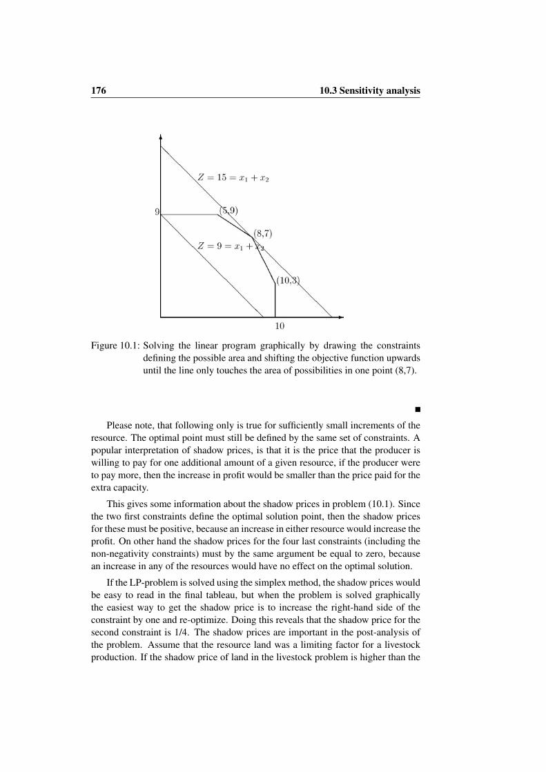
176 10.3 Sensitivity analysis
Figure 10.1: Solving the linear program graphically by drawing the constraintsdefining the possible area and shifting the objective function upwardsuntil the line only touches the area of possibilities in one point (8,7).
Please note, that following only is true for sufficiently small increments of theresource. The optimal point must still be defined by the same set of constraints. Apopular interpretation of shadow prices, is that it is the price that the producer iswilling to pay for one additional amount of a given resource, if the producer wereto pay more, then the increase in profit would be smaller than the price paid for theextra capacity.
This gives some information about the shadow prices in problem (10.1). Sincethe two first constraints define the optimal solution point, then the shadow pricesfor these must be positive, because an increase in either resource would increase theprofit. On other hand the shadow prices for the four last constraints (including thenon-negativity constraints) must by the same argument be equal to zero, becausean increase in any of the resources would have no effect on the optimal solution.
If the LP-problem is solved using the simplex method, the shadow prices wouldbe easy to read in the final tableau, but when the problem is solved graphicallythe easiest way to get the shadow price is to increase the right-hand side of theconstraint by one and re-optimize. Doing this reveals that the shadow price for thesecond constraint is 1/4. The shadow prices are important in the post-analysis ofthe problem. Assume that the resource land was a limiting factor for a livestockproduction. If the shadow price of land in the livestock problem is higher than the

10.3 Sensitivity analysis 177
Figure 10.2: The change in price of x1 causes the slope of the profit line to change,but only the change from p1 = 1 to p1 = 3 causes the optimal pro-duction mix to change from the old optimum (8,7) to (10, 3).
expected return for the crop currently occupying some of the farmers land, then theproduction plan should be altered to allow for land utilized by livestock.
10.3.2 Price adjustments
Assume that the price of x1 suddenly increases due to a change in the demand. Thequestion is: does this call for modifications of the optimal combination of x1 andx2? The answer is maybe! It depends on how much the price increases. This isillustrated in Figure 10.2. It is seen that an increase from p1 = 1 to p1 = 11
2 causeno changes, but an increase to p1 = 3 makes the optimal solution change from(8,7) to (10,3).
Figure 10.2 shows that the slope of the profit line becomes steeper and steeperas the price of x1 increases. The value of p1 that cause the optimum to shift from(8,7) to (10,3) is the value that makes the slope of the profit line equal the slope ofthe constraint 2x1 + x2 ≤ 23. The same result makes the optimum change from(8,7) to (5,9) when the price of x1 is decreased enough to make the slope of theprofit line equal that of the constraint 2x1 + 3x2 ≤ 37. This means, that as longas the price of x1 is within the interval 2/3 to 2 (and the price of x2 is fixed) theoptimum will remain unchanged. The corresponding number for changes in theprice of x2 is 1/1 to 3/2 for p1 fixed.

178 10.3 Sensitivity analysis
Analysis like this is important to estimated the stability of the solution. Ifminor changes in certain parameters would cause the optimum to shift from onepoint to another, then fluctuations in these parameters should be monitored moreintensively in order to make the necessary adjustments.
10.3.3 Capacity changes
When changing the capacity of a given resource the same questions as in the previ-ous section arise. Will this affect the current optimal solution? Again, the answerdepends on how much the capacity is changed. From our discussion of shadowprices it is clear, that an increase in the capacity of a resource that is currently nota limiting factor will have no effect on the current solution. This situation is hardlyof any interest in practical applications, but the reverse situation is very interesting:how much can I reduce this factor, and still keep the current solution? The answeris: as long as the resource is not a limiting factor, i.e. when the current solutiongets infeasible if the resource is reduced further.
If (x∗1, x∗2) is the optimal solution, then the surplus capacity of resource i is
calculated as:
bi − (ai1x∗1 + ai2x
∗2)
i.e. the right-hand side minus the allocated activities.If the surplus capacity is zero, then the resource is a limiting factor, i.e. the
constraint helps define the solution. Any changes in such a factor would causethe optimal production to change, but the question is then how much can a limitingresource be increased (or decreased) without changing the set of limiting resources.
In this graphic approach this is done much like finding the optimum solutionby shifting the profit line. The constraint is simply shifted parallel upwards anddownwards until other constraints becomes limiting factors. This is done in Figure10.3 where the result is that the capacity of the constraint 2x1 + 3x2 ≤ 37 can bebetween 29 and 39 without changing the set of limiting factors.
10.3.4 Additional constraints
When adding extra constraints to an LP-problem, two different scenarios occur:either the constraint is fulfilled by the current optimal solution, hence this is stillthe optimal solution, or the current optimal solution is no longer a feasible solution(i.e. the point where the solution was obtained is violating the new constraint). Theway to deal with additional constraints in the graphical solution procedure is simplyto add the constraint by drawing the corresponding line and then see whether or notthe solution is still optimal. The two different situations are shown in Figure 10.4.

10.3 Sensitivity analysis 179
Figure 10.3: The change in capacity cause the shifts from the optimal solution (8,7) to (7, 9) for capacity above 39 or (10,3) for capacities below 29.
Figure 10.4: Adding the constraint x1 +x2 ≤ 16 has no effect on the optimal solu-tion, but adding x1 + x2 ≤ 13 makes the current optimum infeasibleand the new optimum is (10,3).

180 10.4 Concluding remarks
10.4 Concluding remarks
The art of designing LP-models as decision support tools has been by applied to alot of different problems in the field of herd management. Classic examples includenutrient management (Henry et al., 1995), ration formulation (Gonzales-Alcortaet al., 1994) and selection of sire portfolios (Nash and Rogers, 1995). These areonly a very few of the examples found in literature.
The most important feature of any decision support system is a solid modelvalidation. The extensive theory regarding sensitivity analysis enables a methodicvalidation of LP-models. An implication of this result is that building an initialmodel using LP-techniques will help the modeler to understand the basic interac-tions of the involved resources and decisions.
Because of the wide range of applications several possibilities for modeling andsolving LP-models exist. Any modern spreadsheet will provide a method for for-mulating and solving LP-models of reasonable size. The LINDO software packageis a tool for solving LP-problems, it is especially well suited for use from withina user interface. The probably most powerful mathematical modeling softwareavailable is the GAMS package, which is a combination of modeling language anda series of solvers capable of linear programming, mixed-integer programming,non-linear programming and much more. It is recommended to use GAMS if themodel will be large because of the high quality solvers available to GAMS. Forinitial trials a spreadsheet will prove sufficient.
10.5 Exercise
To check the understanding of the discussed topics consider the following small ex-ercise, which essentially originates from Dent et al. (1986): Robert McCull owns200 ha of irrigated pasture, for which carrying capacities have been estimated to beas follows:
Breeding ewe flock Spring/summer fattening of cattle(ewes per ha) (steers per ha)
Spring 15 5Summer 24 4Autumn 15 0Winter 8 0
The expected gross margins are $24 per ewe and $60 per steer. Mr McCullwishes to maximize the total farm gross margin.
1. Determine graphically the optimal production program for Mr McCull.
2. Assuming the sheep gross margin remains unchanged at $24 per ewe, by howmuch must the gross margin for steers decline before steer numbers shouldbe reduced? Explain your reasoning.

10.5 Exercise 181
3. Assuming the original gross margin for ewe remains unchanged at $24 perewe, to what must the steer gross margin increase before an increased cattlenumber becomes profitable?
4. Assuming the original gross margin for sheep and cattle of $24 and $60,respectively, calculate the shadow price of spring feed.
5. Mr McCull is considering increasing his winter production by the use of ar-tificial nitrogen fertilizer. He expects that the winter carrying capacity willincrease by 0.1 ewes per hectare for each kilogram of nitrogen applied. As-suming that nitrogen costs $90 per kg, would you recommend that he applynitrogen, and if so, how much? What would your recommendations be ifnitrogen were to cost only $0.2 per kg.

182 10.5 Exercise

Chapter 11
Bayesian networks
Using Bayesian Networks one can easily build a probabilistic expert system incor-porating knowledge of the domain. It consists of two parts: a Directed AcyclicGraph (DAG) specifying the probabilistic interdependencies between the randomvariables and a set of conditional probability tables specifying the strength of thedependencies. Decision graphs discussed in Chapter 12 add decisions- and utilitynodes to the concept.
BNs and DGs give a consistent framework for handling reasoning and decisionmaking under uncertainty. An example could be pregnancy testing of sows. Herefusion of different measurement methods as well as allowing for specification ofsensitivity and specificity in connection with the methods is necessary in order toget an overall result.
Since, a chapter on Bayesian networks has not been written yet, the readers areencouraged to study an excellent textbook by Jensen (2001), where in particularChapters 1 and 2 provide a good introduction to the concept.
For good examples, reference is made to McKendrick et al. (2000b) and Ottoand Kristensen (2004).

184

Chapter 12
Decision graphs: Potential useand current limitations
12.1 Introduction
The purpose of this chapter is to illustrate the potential use of the decision graphtechnique within herd management. Decision graphs were (under the name of In-fluence Diagrams introduced by Howard and Matheson (1981) as a formalism tomodel decision problems with uncertainty for a single decision maker. The influ-ence diagrams gave a more compact graphical representation of a decision problemthan the more traditional decision tree approach. In Shachter (1986) a method wassuggested for solving the decision problem represented by the influence diagramdirectly, without the translation to a decision tree. This method transformed the in-fluence diagram by successively removing nodes in the graph, until at last only onefinal utility node, holding the utility of the optimal policy. In order to solve manysimilar problems one therefore had to start from scratch every time. Shenoy (1992)proposed another algorithm that gave the solution to the influence diagram withoutdisrupting the structure of the diagram. Then Jensen et al. (1994) showed how asimilar approach could be incorporated within the general framework of BayesianNetworks. This approach has been implemented in the Hugin expert system shell.We refer to Jensen et al. (1994) for a presentation of the method. In addition, werefer to the short introduction given in Section 9.6.
As concerns software for decision graphs, reference is made to the Hugin1
system implementing classical influence diagrams under the “no forgetting” as-sumption by use of the strong junction tree approach (Jensen et al., 1994) and theEsthauge LIMID Software System2 implementing Limited Memory Influence Di-agrams as described by Lauritzen and Nilsson (2001).
1http://www.hugin.com2http://www.esthauge.dk

186 12.2 From decision tree to influence diagram
12.2 From decision tree to influence diagram
The decision tree is a method for decision analysis. An excellent general descrip-tion can be found in Hillier and Lieberman (1996). The concept is also illustrated inExample 5 of Chapter 4. In order to further illustrate the method we will elaborateon the pregnancy diagnoses decision tree in Figure 9.1 of Chapter 9.
The sequential decisions start from the left of the diagram. A decision node(a square) represents the decision to Make Pregnancy Diagnosis (MPD). From thedecision node two branches originate, “Yes” and “No”. If we follow the “yesbranch”, we encounter a chance node (a circle), the outcome of the pregnancydiagnosis, i.e. either “yes” (positive diagnosis) or “no” (negative). After the chancenode, another decision node is encountered, “Replace” (RP), with “yes” and “no‘”as actions. If we decide to keep the animal, the final chance node is encountered,“Farrowing” (FA) with possible outcomes, “yes” or “no”. If we initially decidenot to make pregnancy diagnosis, we have to wait and see what the outcome is atfarrowing time.
At each branching in the nodes, we can assign a utility and a probability. Ifthe pregnancy diagnosis is made, the cost is the additional work. If the animal isreplaced, the income from the slaughter value of the animal plus the expected valueof a new animal is received. If we decide to let the animals farrow, we add the feed-ing cost until farrowing, and the future value of the present animal. If it farrows,we obtain in addition the income from the litter produced. The probability of eachbranching in the chance nodes can be found similarly. If we make a pregnancydiagnosis the probability of the two outcomes depends on the Pregnancy State (PS)of the animal and the precision of the measurement method, but by applying Bayesformula, the probabilities can be found. (Note that the state of nature, PS, is notrepresented in the diagram). Similarly the probability of farrowing given PS andPD can be found and assigned to each branch leading from FA. To solve the deci-sion tree diagram, one starts from the outmost branches (the leaves). In a chancenode we calculate the expected utility. I.e. the expected utility in the FA node isthe probability of farrowing times the income from a litter plus the probability ofnot farrowing times the income from not producing a litter (0). At a decision nodewe use maximizing instead of taking the expectation. I.e. we make the decisionthat have the highest expected utility. Gradually we move from the leaves to thestem/root of the decision tree.
As a real tree, the decision tree very soon becomes confusing to look at, i.e.the idea behind the graphic representation is soon lost. Furthermore, we had to dosome calculations outside the tree, because some of the chance nodes were not rep-resented (i.e. the pregnancy state). In addition some chance node are representedat several places in the diagram (e.g. the FA node)
The Influence diagram solved these problems to a large degree, when they wereintroduced by Howard and Matheson (1981). The use of the circle as a symbol fora chance node, and the square for a decision node was maintained, but in addi-tion the diamond was added to represent the utility in the diagram. The branches

12.3 From Bayesian network to influence diagram 187
that represented the outcomes of decisions/chances, were removed and replacedby arrows that showed what influenced the decisions and chance nodes. The util-ity representation of the pregnancy diagnosis problem is also shown in Figure 9.1.The chance node PS (Pregnancy State) is added. The MPD node influences thenode UD (Utility Diagnosis), and the outcome of the pregnancy diagnosis, and thenext decision RP. The outcome of the pregnancy diagnosis is in addition influencedby the PS node. Note that PS influences FA directly disregarding the outcome ofPD. The utility from replacement (UR) and from farrowing (UF) finishes the pic-ture. (Strictly speaking, in the original approach only one mutual utility node waspresent).
Originally the influence diagrams were automatically translated to decisiontrees and solved using the same algorithm as mentioned above. Shachter (1986)showed how the influence diagram could be solved directly by removing nodes sub-sequently, based on 4 different transactions, the arc reversal (application of BayesTheorem), node removal by summing out, expectation of a value node with re-spect to a chance node, and finally removal of a decision node into a value node bymaximization. The first attempts were based on discrete valued state variables, butShachter and Kenley (1989) implemented influence diagrams for Gaussian (nor-mal) distributed variables.
12.3 From Bayesian network to influence diagram
If we look at the graphic representation of the decision graphs and compare withthe Bayesian network, we find that they have the same nodes, i.e. the chancenodes, represented as circles. The two additional elements in decision graphs, thedecision variables (squares) and utility functions (diamonds), can in fact also behandled within the framework of Bayesian networks by putting some restrictionson the solution method. This was first shown in Jensen et al. (1994). In fact, ifthe subsequent decisions are not sequential (i.e. the result of a previous decisiondoes not influence other decisions) they can be directly represented in the Bayesiannetwork by using the calculation trick, shown in Jensen (1996, Chapter 6). Inrealistic decision problems this is seldom the case.
The exact procedure for solving influence diagrams as it has been implementedin HUGIN, can be found in Jensen et al. (1994). Here we will summarize themethod based on the diagram in Figure 9.1. An important difference betweenBayesian networks and influence diagrams is the dynamic aspect, i.e. the se-quential decisions impose an ordering on the elements. First of all, the decisionsare ordered according to the sequence in which they are performed, ie. UD =MPD,RP in this case. The ordering is secured by putting directed edges be-tween the decision nodes on the graph. Second, the chance nodes are put intosequential groups as well, i.e UR = I0, I1, I2, where I0 is the set of observationsbefore the first decision (in this case it is empty), I1 is the set of observations be-tween the first and the second decision, i.e. I1 = PD, and finally the nodes that

188 12.4 From Dynamic Programming to influence diagrams
are observed after the second decision or never observed, i.e. I2 = PS, FA. Wethus obtain a partial ordering,
∅ ≺ MPD ≺ PD ≺ RP ≺ PS, FA.
In Bayesian networks, the approach, as described in Jensen (1996, Section 4.5),would be to make a junction tree from the graph, by moralizing and triangulatingthe graph. In this case, however, a so-called strong junction tree is made. Thismeans that the ordering, we have made, should be preserved in the junction tree,implying that the variables at the right should be eliminated before the variables onthe left.
This ordering, which is a consequence of the “no forgetting” assumption dis-cussed in Section 9.6, means that the computational complexity of influence di-agrams with decision nodes in general is much larger than in Bayesian networkswithout.
As described in Jensen et al. (1994) we can then use the junction tree for prop-agation of evidence by simply interchanging maximization for calculation of ex-pectation.
One note of caution is that the ordering should be preserved in the subsequentcalculations made by in the network. In standard Hugin, evidence can be enteredanywhere in the tree, and the evidence is distributed properly. This is not possiblewith influence diagrams. For example, it does not make sense to study the effectof a known pregnancy state, because evidence of pregnancy state is defined onlyto be available after all decisions have been made. Similarly the effect of knownoutcome of pregnancy diagnosis can only be studied for given level of the decisionMPD. Unfortunately, the program does not have a facility that checks that evidenceis input in the correct sequence. However, if the decisions are assigned fixed valuesthe evidence can be entered.
The rather new concept of LImited Memory Influence Diagrams described byLauritzen and Nilsson (2001) relaxes the “no forgetting” assumption as mentionedin Section 9.6. The solution algorithm for this class of models is called SinglePolicy Updating, and all calculations are done in an ordinary junction tree justlike those used with Bayesian networks (i.e. a strong junction tree is not needed).From a computational point of view, LIMIDs are therefore very appealing, but onthe cost of exactness. In many cases, Single Policy Updating only leads to near-optimal solutions, even though they in most cases are very close to the optimum.
12.4 From Dynamic Programming to influence diagrams
The central paper in this respect is Tatman and Shachter (1990). Until the pub-lication of their paper, influence diagrams were constructed with only one utilitynode. They showed that if the utility function was separable, i.e. either additive ormultiplicative, the influence diagram technique corresponded to the Dynamic Pro-

12.4 From Dynamic Programming to influence diagrams 189
Figure 12.1: Influence Diagram representing part of the replacement problem forsows. LS_i is litter size in parity i, Dx represents decisions and Uxutility.
gramming method, i.e. Dynamic Programming is a special case of the influencediagram method.
Because of the more flexible approach towards representing the causal rela-tions, the use of influence diagrams could often result in computational savings, byreducing the complexity of the problems.
To illustrate the potential of their techniques, Tatman and Shachter (1990)showed some examples. Their example (B) has close correspondence to the tech-niques used in solving the replacement problem in animal production, as exem-plified by Huirne et al. (1991). Therefore, their example (B) is adapted to thereplacement problem. The core in the replacement model by Huirne et al. (1991)is a model for the relation between litter size in subsequent parities. This can be il-lustrated as in Figure 12.1. (Note that the decision and utility part is not adequatelyrepresented in the figure).
The litter size is observed at subsequent parities and the decision based onthe observation. The litter size is influenced by the litter size in the two previousparities as indicated by the arrows. Each litter size node has some 20 differentlevels (0, . . . , 19).
To solve this in standard dynamic programming, Huirne et al. (1991) used stateaugmentation, i.e. they made a state variable consisting of (LS_i, LS_i + 1), asillustrated in the next figure, i.e. the state variable had 202 = 400 states. Thiscorresponds to the influence diagram in Figure 12.2.
The resulting transition matrix consisted of 400× 400 = 160, 000 elements. Ifthe influence diagram shown if Figure 12.1 was used directly, the problem wouldonly consist of matrices of 20× 400 = 8000 elements. If information from furtherprevious litters were included, the difference would be even more pronounced. It

190 12.5 Examples
Figure 12.2: Representation of the state augmentation, LS_ij is the combined statevariable of litter size in parity i and j.
is worth noting that this reduction in dimensionality is unrelated to the reductionsdue to hierarchic Markov processes (cf. Section 13.3.2). Similar savings in statespace is expected in representing other independent components of the state space,e.g. state for pregnancy ability (number of re-matings).
However, in the current framework of decision graphs, only problems with fi-nite planning horizon can be solved, as every time step has to be represented in thediagram. Furthermore, the use of semi-Markov processes rather than Markov pro-cesses, with the resulting flexibility in using different time scales has not been im-plemented either. Finally, the advantages of the hierarchic Markov process, wherein fact a decision can select a process with a different causal structure is not yetpossible.
12.5 Examples
The following is a presentation of examples of the possibility for using influencediagrams. The examples have not been constructed in detail but the overall struc-ture of the decision problem should be clear, and quantification of the elements inthe example should be possible. The intention is to stimulate ideas for applicationof the technique within animal production.
12.5.1 The two-sow problem
We shall once again return to the “two-sow prolem” introduced in Example 20 ofChapter 6. As the reader will probably remember, a pig producer has bought twosows with the same expected farrowing date. One of the sows has to be culledbecause there is only room for one sow in the farrowing department. The litter size

12.5 Examples 191
Figure 12.3: Influence diagram representation of the two sow problem.
of a sow is correlated with the litter size in her previous litter. Information aboutthe litter size in the previous litter can be bought from the farmer, who sold the twosows. How much should he be willing to pay for the information, and which sowshould he keep?
The example can be formulated as an influence diagram as shown in Figure12.3. The litter size LSi of sow i depends on the previous litter size PLSi. We candecide to observe i.e. buy the information concerning the previous litter size, andobtain Observed Litter Size (OLSi). Based on the observed value we can decidewhich of the sows we should keep, and the resulting litter size is kept in the nodeLS.
12.5.2 The registration problem for the whole cycle
In fact the registration problem does not only concern the previous litter size, butalso the use of heat-detection, pregnancy diagnosis etc. We can easily add nodesfor Heat detection, Pregnancy diagnosis and the corresponding decision nodes andutility nodes to the diagram as shown in Figure 12.4 for the one sow case.
The decision nodes are UHD (use heat detection), UPD (use pregnancy diag-nosis), and ULS (use litter size information). To each decision a utility node hasbeen assigned. An additional chance node has been assigned, PS, representingpregnancy state. The network in 12.4 can be seen as a combination of Figure 9.1and 12.3.
In Figure 12.5 the decision example is specified for the two sow problem. Inaddition nodes for herd level of pregnancy rate (HPR), heat detection rate (HDR)and efficiency of pregnancy diagnosis (Herdetect) has been added. These nodeswill represent the uncertainty in the parameters used in the calculation. In addition

192 12.5 Examples
Figure 12.4: Influence diagram representing the decisions in a whole gestation pe-riod for a single sow.
the nodes will make the system “learn” from the observations made. A trick is usedto ease the specification of the conditional probabilities. The nodes HDi, PDi andPLSi represent the outcome of the observations. Additional nodes XXOi representthe information that decisions are based upon, e.g. if a pregnancy diagnosis isperformed the states of PDO will be identical to the state of PD. If observations arenot made, the state “Not observed” of PDO will have probability 1, i.e. the variablecontains no information about the true state.
The network in Figure 12.5 is an example of a network that should be usedcautiously when entering evidence. The herd pregnancy rate is one of the nodes,where it would be tempting to ask: What if the pregnancy rate was 0.75, whatwould the optimal decision be. This is not allowed, because herd pregnancy rate isdefined as an unobservable node, i.e. it does not influence any decision.
Note also that the complexity of Figure 12.5. Even with as few as two animalsin the network, the decision graph is not readily understood. Of course the problemcan be generalized to three sows, but now the diagram becomes almost impossibleto understand. A method exists for easy representation of replicated processes,the so-called frames where a rectangular box around part of the network signifythat this part of the network is to be replicated. This approach is eg. used in thespecification in BUGS3 (Gilks et al., 1993). This to some extent solves the problemof too complicated networks, and is especially suited for automatic learning withinthe network (Buntine, 1994). Such a representation for the network is shown in12.6. Unfortunately this technique cannot yet be used within Hugin.
3The BUGS programme and manual can be found by visiting the web-adress with URL:http://www.mrc-bsu.cam.ac.uk/bugs/

12.5 Examples 193
Figure 12.5: Influence diagram representing the decisions within gestation for twosows.
Figure 12.6: Frame representation of the general N-sow problem. Nodes withinthe frame is replicated automatically. (not yet possible within Hugin).

194 12.5 Examples
Figure 12.7: Representing model for litter size with additive effect of sow, A.
Another aspect is the computational complexity. Already with a few sows theproblem becomes difficult to handle on a standard PC. As the complexity increasesexponentially with the number of animals, clearly any computer will be overbur-dened if realistic problems are to be solved. Therefore, approximate methods needto be implemented within the diagram. In a similar framework, considering opti-mal number of sows mated, Greve (1995) implemented a heuristic algorithm andwas able to solve problems of realistic size, i.e. herd sizes in excess of 500 sows.
12.5.3 The repeated measurement problem
The dynamic programming model by Huirne et al. (1991) assumed only effect ofthe two previous litters as described in Section 12.4. A more natural approachwould be to assume an additive effect specific for each sow, i.e. a network likeFigure 12.7.
The network corresponds to a statistical model represented as:
LSij = µi +Aj + εij
with µi as the mean of parity i, Aj ∼ N (0, σ2A) as the effect of sow j and εij ∼
N (0, σ2ε) as an independent and random residual.
Using ordinary Bayesian networks such a system can be handled very effec-tively, but not when influence diagrams are used. This is because of the strongjunction tree mentioned earlier. The junction tree without decisions consists ofcliques with A,LSp, and is thus of a moderate size. However as A is an un-observable effect, it has to be included in the last set in the elimination ordering,when the influence diagram is compiled. That is, the triangulation should be madeso thatA can be eliminated before any of the other nodes. This can only be attainedif links are added between litter size in every parity, and then we are back where westarted. The problem shown in Figure 12.7 has a clique in the strong junction treeof size O(N7), where N is the number of state levels in each litter size node. The

12.5 Examples 195
Figure 12.8: Efficient representation of the additive litter size model. A replacedby the observable estimate Ap. Decions are based on Ap.
same problem arises if any other of the current algorithms for solution in influencediagrams is used.
Fortunately, this problem can be circumvented. The trick is to use the underly-ing model to determine observable, Aij values, i.e. estimate of the sow effect basedon results from her previous litters, so that LSi+1,j = µi+1 + β(Aij − µi) + ε.In the case of the model specified, this can easily be found from the multivariatenormal distribution. Then we obtain a network like Figure 12.8 instead. Note thatthe LS nodes are influenced by the estimate. From a causal point of view this ofcourse nonsense, but it provides the correct answer and reduces the complexitydrastically.
In 12.8 we have explicitly specified the learning or estimation process based onthe observations, and based the decision on the learning. As described in Jensen(1996), Bayesian networks are an efficient method for a decision maker to learnposterior distributions from observed data. Therefore it seems a bit surprising thatat the current state of development, when we specify the decision makers subse-quent decisions within the network, we have to presume that he does not use thisefficient learning method, but only bases his decisions on observed values. Thealternative is to specify the learning algorithm directly, as in 12.8.
The figure corresponds to a decision maker that uses a Bayesian network like12.7, as a DSS-tool and base his decisions on the mode of the probability distribu-tion of A after evidence from previous litters has been added to the network.
Further illustration of the possibility for using this updating technique in con-nection with decision support can be found in Kristensen (1993) and Jørgensen(1992). For examples of applications, reference is made to Kristensen and Søllested(2004a,b); Lien et al. (2003).
12.5.4 Optimal timing of matings
After weaning most sows show oestrus/heat within 4 to 6 days. Based on the ob-servation, the manager decides to mate the sow. In order to maximize the resultingconception rate and litter size the general advice is to repeat matings with 12 hoursinterval up to a maximum of three times, if the sow continues to show oestrus. The

196 12.5 Examples
Figure 12.9: Influence diagram representing the problem of optimal timing of mat-ings.
reason for this is that fresh semen (< 24h) should be available around the newlyreleased ovum to increase fertilization success.
Ovulation can, in general, not be observed (see Soede, 1993, for methods forexperimental methods for observing ovulation) and the pig producer has to rely onthe observable signs of heat. Time of ovulation and start of heat are both dependingon the hormonal development that can be summarized as follicular development(it is a complex interaction between the hormones LH, FSH and Oestrogen). Inother words they are conditionally independent given follicle development. Theend of oestrus is determined by follicular development and possible a feed backmechanism from ovulation. An influence diagram with the relevant mechanism isshown in Figure 12.9.
Start of heat (Heatstart) and end of heat (Heatend) is checked at regular inter-vals, e.g. three times a day. The strength of the oestrous signs develops almostfollowing a gaussian curve. Experienced observers will detect weaker oestroussigns than inexperienced, that is, the heat will be observed (O_heatstart) earlieron average. Based on the observed oestrous sign, the pig producer shall decidethe timing and frequency of matings (Mate1, Mate2 and Mate3). Depending onthe timing of matings and the unobserved ovulation time (ovulation) the litter size(LS) will vary. In figure 12.9 the utility nodes are omitted from the mating deci-sions. Further refinements of the diagram would be to include decisions concerningoestrus detection schedule and connected costs.
12.5.5 The feed analysis problem
This example is modified from Pedersen (1996). In dairy production a major partof the feed mix consists of locally produced roughage, such as beets, silage and

12.5 Examples 197
Figure 12.10: Influence diagram representing the problem of optimal timing ofmatings.
straw. Knowledge of the energy contents of the feed is used in e.g. feed budgetingand feed planning. The energy content of roughage can be estimated using severalmethods. The simplest is a table look-up for standard figures for energy content indifferent categories of roughage. Another simple approach is to estimate dry mattercontent and digestibility subjectively, based on experience concerning the look andfeel of the roughage. A more precise evaluation requires a laboratory assessmentof the value. The digestibility can be measured using in vivo techniques that arethe most precise. Alternatively, different in vitro techniques that simulate the invivo techniques can be used to a much reduced price. Other aspects of the feedevaluation can be measured using different techniques, such as NIR.
The dairy farmer thus has to decide, how he should analyze the feed. Beforethis question can be answered, we have to consider the decisions that the feedanalysis influences. In Figure 12.10 this is illustrated.
The roughage has a certain true and unobservable energy content (Energy). Thefarmer can decide to observe the energy level (O_Energy) using different methods(Method). These methods differ in price. Together with the observable energy levelin the roughage and the energy level in the supplement feed (Suplement) the farmerdecides the mixing ratio between these two feed stuffs. The resulting energy in thefeed (E_In_feed) is found based on the mixing ratio and the true energy levels in thetwo feed stuffs. The energy level in the feed will in turn influence the feed intakeand the feed costs (UF). In addition the milk production level will be influenced(UM). As the relative price of the feed analysis increases with decreasing herd size,because the information and the feed mixture are used on fewer animals, the utilityshould be corrected to take this into account. The two nodes Relfeed and Relmilkserve this function.

198 12.6 Outlook
12.6 Outlook
When we judge the possible uses of the decision graphs, we should consider, thatit is a very recent technique, and thus still have some shortcomings.
When we look upon the technique as a generalization of the Markov Chainprocess for Dynamic Programming, the more static approach used in influencediagrams is clearly a constraint. Easy specification of a dynamic system, such asused in dHugin (Kjærulff, 1995) would clearly be a step forward and should makeit possible to utilize techniques comparable to policy iteration. To the authors’knowledge, this has not been developed yet. The flexible time scales, based ondiscounting the utilities, would represent an even further improvement.
The frame approach used in BUGS, see footnote on page 192, would ease thespecification of multi-component systems. It may also be used to represent deci-sion that chooses between qualitatively different subsystems, similar to HierarchicMarkov processes (HMP). The subsystem could be represented as different frames,and the decisions a matter of selecting the frame.
Such developments would make the influence diagram method able to solvesimilar problems as is currently solved by HMP. In addition, savings in complexitysimilar to those described in section 12.4 would be obtained.
The spinoff from the statistical research in Bayesian networks is expected toresult in numerical methods for handling very large systems, as illustrated by theearly attempts by Bielza et al. (1999) and Charnes and Shenoy (1996) to use MonteCarlo techniques to optimize the decision strategies. The savings in complexity bybasing decisions on the learning process in Bayesian networks illustrated in section12.5.3 is another obvious improvement.

Chapter 13
Dynamic programming andMarkov decision processes
13.1 Introduction
13.1.1 Historical development
In the late fifties Bellman (1957) published a book entitled Dynamic Programming.In the book he presented the theory of a new numerical method for the solution ofsequential decision problems. The basic elements of the method are the Bellmanprinciple of optimality and functional equations. The idea may be illustrated asfollows.
Consider a system being observed over a finite or infinite time horizon split upinto periods or stages. At each stage, the state of the system is observed, and adecision (or an action) concerning the system has to be made. The decision influ-ences (deterministically or stochastically) the state to be observed at the next stage,and depending on the state and the decision made, an immediate reward is gained.The expected total rewards from the present stage until the end of the planninghorizon is expressed by a value function. The relation between the value functionat the present stage and the one at the following stage is expressed by the func-tional equation. Optimal decisions depending on stage and state are determinedbackwards step by step as those maximizing the right hand side of the functionalequation. This way of determining an optimal policy is based on the Bellman prin-ciple of optimality which says: An optimal policy has the property that whateverthe initial state and initial decision are, the remaining decisions must constitute anoptimal policy with regard to the state resulting from the first decision (Bellman,1957, p. 83).
During the following years, Bellman published several books on the subject(Bellman, 1961; Bellman and Dreyfus, 1962; Bellman and Kalaba, 1965). Thebooks were very enthusiastic, and the method was expected to be the solution toa very wide range of decision problems of the real world. The expectations were

200 13.1 Introduction
so great, and they were adduced with such a conviction, that Johnston (1965) iron-ically compared dynamic programming to a new religion. Others regarded themethod as a rather trivial computational device.
Similar stories might be told regarding other new numerical methods, as forinstance linear programming. However, after some years, the applicational scopesof the methods are encircled. Most often the conclusion is that the method is neitheran all-embracing technique nor a triviality. Between these extremities a rathernarrow range of problems remains where it is a powerful tool. Other problems are,in some cases, not suitable to be solved by the method. In other cases alternativemethods are better.
This also turned out to be the case in dynamic programming. One of the basicelements of dynamic programming is the sequential approach, which means that itfits sequential decision problems best. Obvious examples of sequential decisionsin animal production include replacement of animals (it is relevant to consider atregular time intervals whether the present asset should be replaced or it should bekept for an additional period), insemination and medical treatment. Dynamic pro-gramming is a relevant tool, but if the traits of the animal are well defined and theirprecise behavior over time is known in advance, there are other methods that mightbe applied to determine the optimal decisions analytically. On the other hand, if thetraits of the animal are affected by random variation over time and among animals,the decisions will depend on the present observations of the traits. In that casedynamic programming is an obvious technique to be used in the determination ofoptimal decisions and policies.
Having identified dynamic programming as a relevant method to be used withsequential decision problems in animal production, we shall continue on the his-torical development. Howard (1960) published a book on Dynamic Programmingand Markov Processes. As will appear from the title, the idea of the book was tocombine the dynamic programming technique with the mathematically well estab-lished notion of a Markov chain. A natural consequence of the combination was touse the term Markov decision process to describe the notion. Howard (1960) alsocontributed to the solution of infinite stage problems, where the policy iterationmethod was created as an alternative to the stepwise backward contraction method,which Howard called value iteration. The policy iteration was a result of the ap-plication of the Markov chain environment and it was an important contribution tothe development of optimization techniques.
The policy iteration technique was developed for two criteria of optimality,namely maximization of total expected discounted rewards and maximization ofexpected average rewards per stage. Later on, Jewell (1963) presented a policy iter-ation technique for the maximization of average rewards over time for semi-Markovdecision processes, which are Markov decision processes of which the stage lengthis a random variable. Howard (1971) presented a value iteration method for semi-Markov decision processes.
For the sake of completeness it should also be mentioned that linear program-ming was early identified as an optimization technique to be applied to Markov

13.1 Introduction 201
decision processes as described by, for instance, Hadley (1964), but no animalproduction models known to the authors have applied that technique. This is in ac-cordance with a conclusion of White and White (1989) that policy iteration (exceptin special cases) is more efficient than linear programming.
Since the publication of the first mentioned book by Howard (1960) an in-tensive research in Markov decision programming has been carried out. Manyresults have been achieved concerning the relations between the various optimiza-tion techniques and criteria of optimality. Reviews of these developments are givenby van der Wal and Wessels (1985) as well as White and White (1989).
13.1.2 Applications in animal production
The dominant area of application in animal production has been for solving theanimal replacement problem either alone or in connection with insemination andmedical treatment. It is however expected that recent methodological develop-ments will broaden the applicational scope.
Already three years after the book by Howard (1960), an application to thedairy cow replacement problem was published by Jenkins and Halter (1963). Theirmodel only included the trait “lactation number” (at 12 levels), and the permanentvalue of the study was only to illustrate that Markov decision programming is apossible tool to be applied to the problem. A few years later, however, Giaever(1966) published a study which represents a turning-point in the application of themethod to the animal (dairy cow) replacement problem. He considered all threeoptimization techniques (value iteration, policy iteration and linear programming),described how to ensure that all mathematical conditions were satisfied, and pre-sented an eminent model to describe the production and feed intake of a dairy cow.The work by Giaever (1966) has not got the credit in literature that it deserves(maybe because it is only available on microfilm). In a review by van Arendonk(1984) it is not even mentioned.
During the following 20 years, several dairy cow replacement models usingMarkov decision programming were published, but from a methodological pointof view none of them have contributed anything new compared to Giaever (1966).Several studies, however, have contributed in other ways. Smith (1971) showedthat the rather small model of Giaever (1966) with 106 states did not representthe upper limit. His state space included more than 15 000 states. Kristensenand Østergaard (1982) as well as van Arendonk (1985, 1986) and van Arendonkand Dijkhuizen (1985) studied the influence of prices and other conditions on theoptimal replacement policy. Other studies (Killen and Kearney, 1978; Reenberg,1979) hardly reached the level of Jenkins and Halter (1963).
Even though the sow replacement problem is almost identical to that of dairycows, very few early studies on sows have been published. The only exceptionsknown to the authors are Huirne et al. (1988, 1991, 1993) and Jørgensen (1992).
A study by Ben-Ari et al. (1983) deserves special attention. As regards method-ology it is not remarkable, but in that study the main difficulties concerning appli-

202 13.2 Variability and cyclic production: Markov decision programming
cation to animal production models were identified and clearly formulated. Threefeatures were mentioned:
Uniformity: The traits of an animal are difficult to define and measure. Further-more the random variation of each trait is relatively large.
Reproductive cycle: The production of an animal is cyclic. It has to be decidedin which cycle to replace as well as when to replace inside a cycle.
Availability: Only a limited supply of replacements (in that case heifers) is avail-able.
The first feature in fact covers two different aspects, namely uniformity becausethe traits are difficult to define and measure, and variability because the traits varyat random among animals and over time. The third feature is an example of aherd restraint, i.e. a restriction that applies to the herd as a whole and not to theindividual animal. Other examples of herd restraints are a production quota or alimited housing capacity. We shall therefore consider the more general problem ofherd restraints.
We may conclude that until the mid-eighties, the methodological level concern-ing the application of Markov decision programming to animal production modelswas represented by Giaever (1966). The main difficulties that the method shouldovercome had been identified by Ben-Ari et al. (1983). If we compare the approachof Giaever (1966) to the difficulties that it ought to solve, we may conclude thatthe problems related to variability are directly solved, and as it has been shown byKristensen and Østergaard (1982) as well as van Arendonk (1985); van Arendonkand Dijkhuizen (1985); van Arendonk (1986), the problems concerning the cyclicproduction may readily be solved without any methodological considerations. Theonly problem concerning variability and cyclic production is that in order to coverthe variability, the state variables (traits) have to be represented by many levels, andto deal with the cyclic production a state variable representing the stage of the cyclehas to be included. Both aspects contributes significantly to an explosive growth ofthe state space. We therefore face a dimensionality problem. Even though all nec-essary conditions of a Markov decision process are met, the solution in practice isprohibitive even on modern computers. The problems concerning uniformity andherd restraints are not solved by the approach of Giaever (1966).
13.2 Variability and cyclic production: Markov decisionprogramming
As mentioned in the introduction, Markov decision programming is directly ableto take the variability in traits and the cyclic production into account without anyadaptations. In order to have a frame of reference, we shall briefly present the the-ory of traditional Markov decision programming originally described by Howard(1960).

13.2 Variability and cyclic production: Markov decision programming 203
Stage 1 Stage 2 Stage 3 Stage 4
Figure 13.1: Stages of a Markov decision process.
13.2.1 Notation and terminology
Consider a discrete time Markov decision process with a finite state space U =1, 2, ..., u and a finite action set D. A policy, s is a map assigning to each statei ∈ U an action s(i) ∈ D. Let pd
ij be the transition probability from state i tostate j if the action d ∈ D is taken. The reward to be gained when the state i isobserved, and the action d is taken, is denoted as rd
i . The time interval betweentwo transitions is called a stage.
We have now defined the elements of a traditional Markov decision process,but in some models we further assume that if state i is observed, and action d istaken, a physical quantity of md
i is involved (e.g. Kristensen, 1989, 1991). In thisstudy we shall refer to md
i as the physical output. If s(i) = d, the symbols rdi , md
i
and pdij are also written as rs
i , msi and ps
ij , respectively.An optimal policy is defined as a policy that maximizes (or minimizes) some
predefined objective function. The optimization technique (i.e. the method to iden-tify an optimal policy) depends on the form of the objective function or - in otherwords - on the criterion of optimality. The over-all objective to maximize net rev-enue of the entire herd may (depending on the circumstances) result in differentcriteria of optimality formulated as alternative objective functions. The choice ofcriterion depends on whether the planning horizon is finite or infinite.
13.2.2 A simple dairy cow replacement model
For any dairy cow it is relevant to consider at regular time intervals whether itshould be kept for an additional period or it should be replaced by a heifer. If theline of Figure 13.1 represents time, the markers indicate where we consider to re-place. The time interval between two markers is called a stage and in this examplewe assume the stage length to be one year which for convenience is assumed al-ways to be equal to a lactation period. At the beginning of each stage, we observethe state of the animal in production. The state space must be defined in such waythat all relevant information is given by the state. In this very simple example weassume, that the only relevant information is whether the cow is low, average orhigh yielding. Thus we have got one state variable (milk yield) and three states.
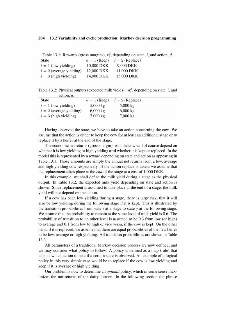
204 13.2 Variability and cyclic production: Markov decision programming
Table 13.1: Rewards (gross margins), rdi , depending on state, i, and action, d.
State d = 1 (Keep) d = 2 (Replace)i = 1 (low yielding) 10,000 DKK 9,000 DKKi = 2 (average yielding) 12,000 DKK 11,000 DKKi = 3 (high yielding) 14,000 DKK 13,000 DKK
Table 13.2: Physical outputs (expected milk yields), mdi , depending on state, i, and
action, d.State d = 1 (Keep) d = 2 (Replace)i = 1 (low yielding) 5,000 kg 5,000 kgi = 2 (average yielding) 6,000 kg 6,000 kgi = 3 (high yielding) 7,000 kg 7,000 kg
Having observed the state, we have to take an action concerning the cow. Weassume that the action is either to keep the cow for at least an additional stage or toreplace it by a heifer at the end of the stage.
The economic net returns (gross margin) from the cow will of course depend onwhether it is low yielding or high yielding and whether it is kept or replaced. In themodel this is represented by a reward depending on state and action as appearing inTable 13.1. Those amounts are simply the annual net returns from a low, averageand high yielding cow respectively. If the action replace is taken, we assume thatthe replacement takes place at the end of the stage at a cost of 1,000 DKK.
In this example, we shall define the milk yield during a stage as the physicaloutput. In Table 13.2, the expected milk yield depending on state and action isshown. Since replacement is assumed to take place at the end of a stage, the milkyield will not depend on the action.
If a cow has been low yielding during a stage, there is large risk, that it willalso be low yielding during the following stage if it is kept. This is illustrated bythe transition probabilities from state i at a stage to state j at the following stage.We assume that the probability to remain at the same level of milk yield is 0.6. Theprobability of transition to an other level is assumed to be 0.3 from low (or high)to average and 0.1 from low to high or vice versa, if the cow is kept. On the otherhand, if it is replaced, we assume that there are equal probabilities of the new heiferto be low, average or high yielding. All transition probabilities are shown in Table13.3.
All parameters of a traditional Markov decision process are now defined, andwe may consider what policy to follow. A policy is defined as a map (rule) thattells us which action to take if a certain state is observed. An example of a logicalpolicy in this very simple case would be to replace if the cow is low yielding andkeep if it is average or high yielding.
Our problem is now to determine an optimal policy, which in some sense max-imizes the net returns of the dairy farmer. In the following section the phrase

13.2 Variability and cyclic production: Markov decision programming 205
Table 13.3: Transition probabilities from state i at a stage to state j at the followingstage.
State at present stage d = 1 (Keep) d = 2 (Replace)j = 1 j = 2 j = 3 j = 1 j = 2 j = 3
(L) (A) (H) (L) (A) (H)i = 1 (L) 0.6 0.3 0.1 0.333 0.333 0.333i = 2 (A) 0.2 0.6 0.2 0.333 0.333 0.333i = 3 (H) 0.1 0.3 0.6 0.333 0.333 0.333
“in some sense maximizes” is clarified. Afterwards, a survey of optimization tech-niques is given. Throughout the discussion we shall refer to this numerical exampleas the simple dairy model.
13.2.3 Criteria of optimality
Finite planning horizon
A farmer, who knows that he is going to terminate his production after N stages,may use the maximization of total expected rewards as his criterion of optimality.The corresponding objective function h is
h(s1, ..., sN ) = E
(N∑
n=1
rsn
I(n)
), (13.1)
where E denotes the expected value, sn is the policy at stage n, and I(n) is the (un-known) state at stage n. Applying this criterion to the simple dairy model meansthat the the total expected net returns over a fixed number (N ) of years are maxi-mized.
If the farmer has a time preference, so that he prefers an immediate reward toan identical reward later on, a better criterion is the maximization of total expecteddiscounted rewards. If all stages are of equal length, this is equal to applying theobjective function
h(s1, ..., sN ) = E
(N∑
n=1
βn−1rsn
I(n)
), (13.2)
where 0 < β < 1 is the discount factor defined by the interest rate and the stagelength.
Infinite planning horizon
A situation where the stage of termination is unknown (but at least far ahead) isusually modeled by an infinite planning horizon (i.e. N = ∞). In that case theoptimal policy is constant over stages. The function 13.1 cannot be applied in this

206 13.2 Variability and cyclic production: Markov decision programming
situation, but since β < 1, the function 13.2 will converge towards a fixed valuefor N becoming very large. Thus the objective function is given by
h(s) = E
( ∞∑n=1
βn−1rsI(n)
). (13.3)
Since, usually, each animal and its future successors are represented by a sep-arate Markov decision process, this criterion together with the criterion 13.2, areequal to the maximization of total discounted net revenues per animal. Such a cri-terion is relevant in a situation where a limiting housing capacity is the only (or atleast the most limiting) herd restraint.
An alternative criterion under infinite planning horizon is the maximization ofexpected average reward per unit of time. If all stages are of equal length, theobjective function in this situation is
h(s) = gs =u∑
i=1
πsi r
si , (13.4)
where πsi is the limiting state probability under the policy s (i.e. when the policy
is kept constant over an infinite number of stages). This criterion maximizes theaverage net revenues per stage, i.e. over time. In the simple dairy model, appli-cation of this criterion indicates that average annual net returns are maximized. Itmay be relevant under the same conditions as criterion 13.3 if an animal and itsfuture successors are represented by a separate Markov decision process. Practicalexperience shows that the optimal replacement policies determined under criteria(13.3) and (13.4) are almost identical.
If a herd restraint (e.g. a milk quota) is imposed on the physical output, arelevant criterion may be the maximization of expected average reward per unit ofphysical output using the objective function
h(s) = gs =gsr
gsm
=∑u
i=1 πsi r
si∑u
i=1 πsim
si
. (13.5)
In case of a milk quota, the physical output msi is the milk produced by a
cow in state i under policy s, and accordingly, average net returns per kg milk ismaximized in the simple dairy model. The function 13.5 is also relevant if thecriterion is the maximization of the expected average reward over time in a modelwhere the stage length varies. In that case the physical output represents the stagelength. It should be noticed that if md
i = 1 for all i and d, the function 13.5 isidentical to 13.4. The symbol gs
r is the average reward over stages (equal to gs ofEq. (13.4)) and gs
m is the average physical output over stages.
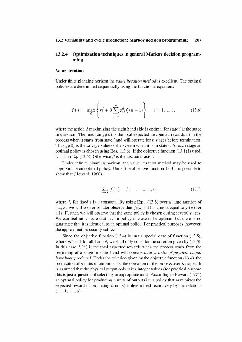
13.2 Variability and cyclic production: Markov decision programming 207
13.2.4 Optimization techniques in general Markov decision program-ming
Value iteration
Under finite planning horizon the value iteration method is excellent. The optimalpolicies are determined sequentially using the functional equations
fi(n) = maxd
rdi + β
u∑j=1
pdijfj(n− 1)
, i = 1, ..., u, (13.6)
where the action d maximizing the right hand side is optimal for state i at the stagein question. The function fi(n) is the total expected discounted rewards from theprocess when it starts from state i and will operate for n stages before termination.Thus fi(0) is the salvage value of the system when it is in state i. At each stage anoptimal policy is chosen using Eqs. (13.6). If the objective function (13.1) is used,β = 1 in Eq. (13.6). Otherwise β is the discount factor.
Under infinite planning horizon, the value iteration method may be used toapproximate an optimal policy. Under the objective function 13.3 it is possible toshow that (Howard, 1960)
limn→∞
fi(n) = fi, i = 1, ..., u, (13.7)
where fi for fixed i is a constant. By using Eqs. (13.6) over a large number ofstages, we will sooner or later observe that fi(n + 1) is almost equal to fi(n) forall i. Further, we will observe that the same policy is chosen during several stages.We can feel rather sure that such a policy is close to be optimal, but there is noguarantee that it is identical to an optimal policy. For practical purposes, however,the approximation usually suffices.
Since the objective function (13.4) is just a special case of function (13.5),where ms
i = 1 for all i and d, we shall only consider the criterion given by (13.5).In this case fi(n) is the total expected rewards when the process starts from thebeginning of a stage in state i and will operate until n units of physical outputhave been produced. Under the criterion given by the objective function (13.4), theproduction of n units of output is just the operation of the process over n stages. Itis assumed that the physical output only takes integer values (for practical purposethis is just a question of selecting an appropriate unit). According to Howard (1971)an optimal policy for producing n units of output (i.e. a policy that maximizes theexpected reward of producing n units) is determined recursively by the relations(i = 1, . . . , u):
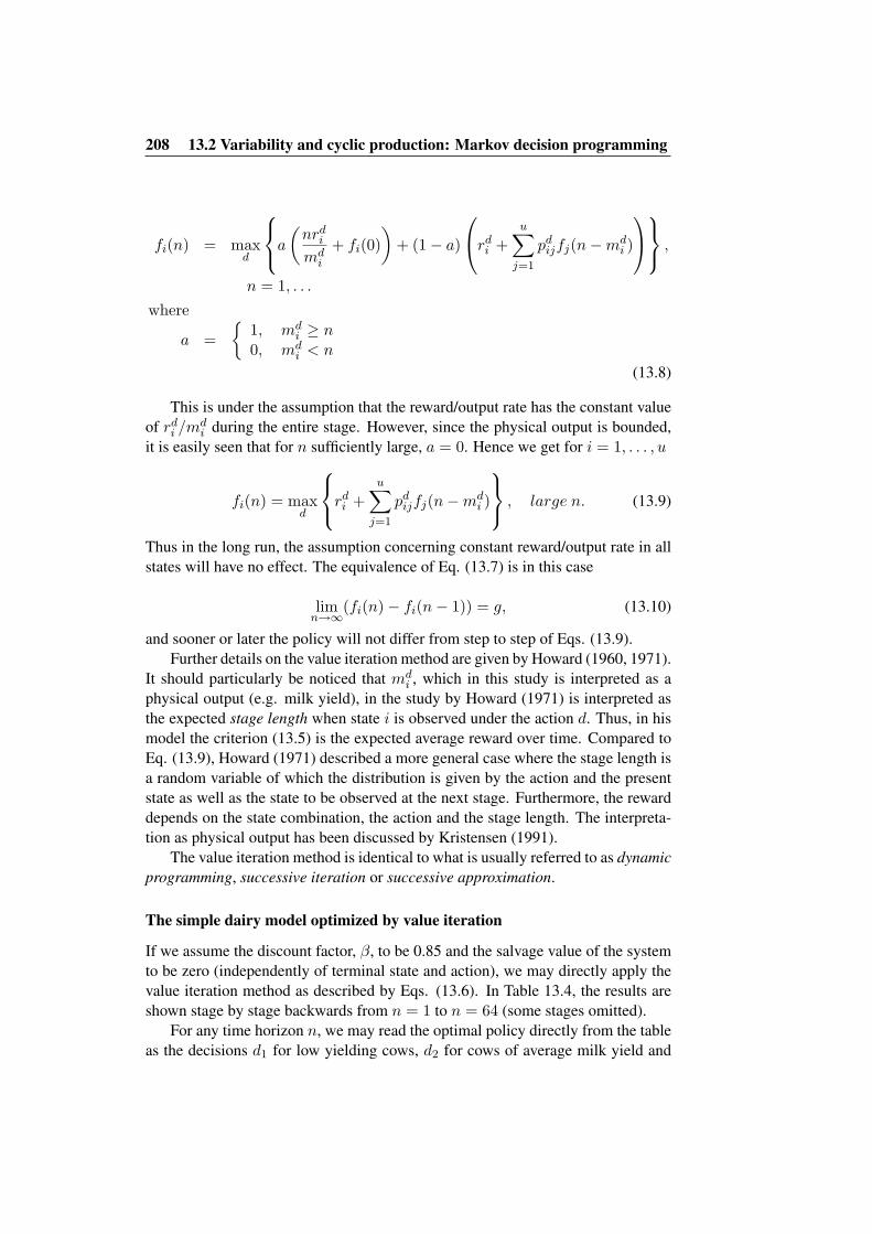
208 13.2 Variability and cyclic production: Markov decision programming
fi(n) = maxd
a(nrd
i
mdi
+ fi(0))
+ (1− a)
rdi +
u∑j=1
pdijfj(n−md
i )
,
n = 1, . . .where
a =
1, mdi ≥ n
0, mdi < n
(13.8)
This is under the assumption that the reward/output rate has the constant valueof rd
i /mdi during the entire stage. However, since the physical output is bounded,
it is easily seen that for n sufficiently large, a = 0. Hence we get for i = 1, . . . , u
fi(n) = maxd
rdi +
u∑j=1
pdijfj(n−md
i )
, large n. (13.9)
Thus in the long run, the assumption concerning constant reward/output rate in allstates will have no effect. The equivalence of Eq. (13.7) is in this case
limn→∞
(fi(n)− fi(n− 1)) = g, (13.10)
and sooner or later the policy will not differ from step to step of Eqs. (13.9).Further details on the value iteration method are given by Howard (1960, 1971).
It should particularly be noticed that mdi , which in this study is interpreted as a
physical output (e.g. milk yield), in the study by Howard (1971) is interpreted asthe expected stage length when state i is observed under the action d. Thus, in hismodel the criterion (13.5) is the expected average reward over time. Compared toEq. (13.9), Howard (1971) described a more general case where the stage length isa random variable of which the distribution is given by the action and the presentstate as well as the state to be observed at the next stage. Furthermore, the rewarddepends on the state combination, the action and the stage length. The interpreta-tion as physical output has been discussed by Kristensen (1991).
The value iteration method is identical to what is usually referred to as dynamicprogramming, successive iteration or successive approximation.
The simple dairy model optimized by value iteration
If we assume the discount factor, β, to be 0.85 and the salvage value of the systemto be zero (independently of terminal state and action), we may directly apply thevalue iteration method as described by Eqs. (13.6). In Table 13.4, the results areshown stage by stage backwards from n = 1 to n = 64 (some stages omitted).
For any time horizon n, we may read the optimal policy directly from the tableas the decisions d1 for low yielding cows, d2 for cows of average milk yield and

13.2 Variability and cyclic production: Markov decision programming 209
Table 13.4: The value iteration method of Eqs. (13.6) applied to the simple dairymodel.
n d1 f1(n) ∆f1(n)∗ d2 f2(n) ∆f2(n)∗ d3 f3(n) ∆f3(n)∗
1 1 10000 10000 1 12000 12000 1 14000 140002 1 19350 9350 1 22200 10200 1 25050 110503 2 27870 8520 1 30870 8670 1 34081 90314 2 35299 7429 1 38275 7405 1 41622 75415 2 41639 6340 1 44597 6322 1 47988 63666 2 47030 5391 1 49981 5384 1 53385 53977 2 51612 4582 1 54561 4580 1 57969 45848 2 55507 3895 1 58455 3894 1 61864 38959 2 58817 3310 1 61765 3310 1 65175 3311
10 2 61631 2814 1 64579 2814 1 67989 281420 2 74437 554 1 77385 554 1 80795 55430 2 76958 109 1 79906 109 1 83316 10940 2 77455 21 1 80402 21 1 83812 2150 2 77552 4 1 80500 4 1 83910 460 2 77572 1 1 80519 1 1 83929 161 2 77572 1 1 80520 1 1 83930 162 2 77573 1 1 80520 1 1 83930 163 2 77573 1 1 80521 1 1 83931 164 2 77574 0 1 80521 0 1 83931 0
∗∆fi(n) = fi(n)− fi(n− 1)

210 13.2 Variability and cyclic production: Markov decision programming
Table 13.5: The value iteration method of Eqs. (13.9) applied to the simple dairymodel.
n d1 f1(n) ∆f1(n)∗ d2 f2(n) ∆f2(n)∗ d3 f3(n) ∆f3(n)∗
1 1 10000 10000 1 12000 12000 1 14000 140002 1 21000 11000 1 24000 12000 1 27000 130003 2 33000 12000 1 36000 12000 1 39500 125004 2 45167 12167 1 48100 12100 1 51800 123005 2 57355 12189 1 60253 12153 1 64027 122276 2 69545 12190 1 72428 12175 1 76228 122017 2 81734 12189 1 84612 12183 1 88420 121928 2 93922 12188 1 96798 12186 1 100609 121899 2 106109 12188 1 108985 12187 1 112797 12188
10 2 118297 12188 1 121172 12187 1 124984 1218811 2 130484 12187 1 133359 12187 1 137172 1218812 2 142672 12187 1 145547 12187 1 149359 1218813 2 154859 12187 1 157734 12187 1 161547 1218714 2 167047 12187 1 169922 12187 1 173734 1218715 2 179234 12187 1 182109 12187 1 185922 12187
∗∆fi(n) = fi(n)− fi(n− 1)
d3 for high yielding cows. If, for instance, we assume a time horizon of n = 10stages, we see that low yielding cows should be replaced whereas average and highyielding cows should be kept. We also observe, that for values of n higher than 3,the optimal policy does not vary over stages.
The columns fi(n) show the expected present value of the chain (i.e. thepresent cow and its future successors), when the present cow is in state i and nstages remain in the time horizon. From the table we observe, that the presentvalues of the three states converges towards fixed values in accordance with Eq.(13.7). Those values appear to be (close to) 77,574 DKK, 80,521 DKK and 83,931DKK for low, average and high yielding cows respectively. The differences be-tween these figures represent the relative values of the three states. For instance,80, 521− 77, 574 = 2, 947 is the economic advantage of having a cow of averagemilk yield instead of a low yielding cow.
In Table 13.5, the corresponding results for the value iteration method underthe criterion (13.4) are shown. The optimal policies appear to be exactly identicalto those of Table 13.4. Under this criterion, however, the value functions fi(n) doesnot converge towards fixed values, because no discounting is involved. Instead, wesee from Table 13.5 that the increments, ∆fi(n) = fi(n)−fi(n−1), in accordancewith Eq. (13.10), converge towards a fixed value of 12,187 DKK independentlyof state. Thus, 12,187 is the numerical value of g, the annual net returns beingmaximized under this criterion.
It is also possible to calculate the economic benefit of, for instance, state 2(average milk yield) over state 1 (low milk yield) from Table 13.5. If we use the
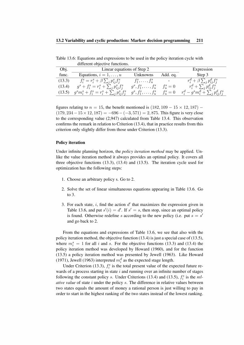
13.2 Variability and cyclic production: Markov decision programming 211
Table 13.6: Equations and expressions to be used in the policy iteration cycle withdifferent objective functions.
Obj. Linear equations of Step 2 Expressionfunc. Equations, i = 1, . . . , u Unknowns Add. eq. Step 3(13.3) fs
i = rsi + β
∑j p
sijf
sj fs
1 , . . . , fsu - rd
i + β∑
j pdijf
sj
(13.4) gs + fsi = rs
i +∑
j psijf
sj gs, f s
1 , . . . , fsu fs
u = 0 rdi +
∑j p
dijf
sj
(13.5) gsmsi + fs
i = rsi +
∑j p
sijf
sj gs, f s
1 , . . . , fsu fs
u = 0 rdi − gsmd
i +∑
j pdijf
sj
figures relating to n = 15, the benefit mentioned is (182, 109 − 15 × 12, 187) −(179, 234− 15× 12, 187) = −696− (−3, 571) = 2, 875. This figure is very closeto the corresponding value (2,947) calculated from Table 13.4. This observationconfirms the remark in relation to Criterion (13.4), that in practice results from thiscriterion only slightly differ from those under Criterion (13.3).
Policy iteration
Under infinite planning horizon, the policy iteration method may be applied. Un-like the value iteration method it always provides an optimal policy. It covers allthree objective functions (13.3), (13.4) and (13.5). The iteration cycle used foroptimization has the following steps:
1. Choose an arbitrary policy s. Go to 2.
2. Solve the set of linear simultaneous equations appearing in Table 13.6. Goto 3.
3. For each state, i, find the action d′ that maximizes the expression given inTable 13.6, and put s′(i) = d′. If s′ = s, then stop, since an optimal policyis found. Otherwise redefine s according to the new policy (i.e. put s = s′
and go back to 2.
From the equations and expressions of Table 13.6, we see that also with thepolicy iteration method, the objective function (13.4) is just a special case of (13.5),where ms
i = 1 for all i and s. For the objective functions (13.3) and (13.4) thepolicy iteration method was developed by Howard (1960), and for the function(13.5) a policy iteration method was presented by Jewell (1963). Like Howard(1971), Jewell (1963) interpreted md
i as the expected stage length.Under Criterion (13.3), fs
i is the total present value of the expected future re-wards of a process starting in state i and running over an infinite number of stagesfollowing the constant policy s. Under Criterions (13.4) and (13.5), fs
i is the rel-ative value of state i under the policy s. The difference in relative values betweentwo states equals the amount of money a rational person is just willing to pay inorder to start in the highest ranking of the two states instead of the lowest ranking.

212 13.2 Variability and cyclic production: Markov decision programming
The absolute value of fsi is determined arbitrarily by the additional equation of Ta-
ble 13.6, where the relative value of state u is defined to be zero. The interpretationof relative values is discussed in details by Kristensen (1991).
Linear programming
Under an infinite planning horizon, linear programming is a possible optimizationtechnique. When the criterion (13.3) is applied, the linear programming problembecomes (Ross, 1970)
u∑i=1
xi = Max!
subject to (13.11)
xi − β
u∑j=1
pdijxj ≥ rd
i , all d ∈ D, i = 1, ..., u .
It appears from 13.11 that each combination of state and action is represented byexactly one restriction. An action d is optimal in state i if, and only if, the corre-sponding restriction is satisfied as an equation when the values of x1, . . . , xu arisesfrom an optimal solution to the linear programming problem. The optimal valuesof x1, . . . , xu are equal to the present values fs
1 , . . . , fsu under an optimal policy.
If the objective function (13.4) is applied, the linear programming problembecomes
u∑i=1
∑d∈D
rdi x
di = Max!
subject to∑d∈D
xdi −
u∑j=1
∑d∈D
pdijx
dj = 0, i = 1, ..., u (13.12)
u∑i=1
∑d∈D
xdi = 1
xdi ≥ 0, d ∈ D, i = 1, ..., u.
In this case an action d is optimal in state i if, and only if, xdi from the optimal
solution is strictly positive. The optimal value of the objective function is equalto the average rewards per stage under an optimal policy. The optimal value of∑
d∈D xdi is equal to the limiting state probability πi under an optimal policy.
Using Criterion (13.5), we may solve the following linear programming prob-lem (Kennedy, 1986):

13.2 Variability and cyclic production: Markov decision programming 213
xu = Max!
subject to (13.13)
−xi +u−1∑j=1
pdijxj −md
i xu ≤ −rdi − pd
iua, d ∈ D, i = 1, ..., u− 1
u−1∑j=1
pdujxj −md
uxu ≤ −rdu − pd
uua+ a, d ∈ D
xi ≥ 0, i = 1, ..., u,
where a is a pre-determined relative value of state u chosen sufficiently large toensure that all other relative values are positive. The optimal value of the objec-tive function of the linear programming problem is equal to the expected averagereward per unit of output as defined in Eq. (13.5) under an optimal policy. Theoptimal values of the variables x1, . . . , xu−1 are equal to the relative values of thestates 1, . . . , u − 1, provided that the relative value of state u is equal to a . Asit appears, each combination of state and action is represented by one, and onlyone, restriction. An action is optimal in a state if, and only if, the correspondingrestriction is satisfied as an equation in the optimal solution.
Since Criterion (13.4) is just a special case of (13.5) with all physical outputsset to the value 1, the linear programming problem (13.13) may also be used in thedetermination of an optimal policy under Criterion (13.4).
13.2.5 Discussion and applications
Under finite planning horizon, the value iteration method is perfect, but in herdmanagement models the planning horizon is rarely well defined. Most often theprocess is assumed to operate over an unknown period of time with no pre-determinedstage of termination. In such cases the abstraction of an infinite planning horizonseems more relevant. Therefore we shall pay specific attention to the optimiza-tion problem under the criteria (13.3), (13.4) and (13.5) where all three techniquesdescribed in the previous sections are available.
The value iteration method is not exact, and the convergence is rather slow.On the other hand, the mathematical formulation is very simple, and the methodmakes it possible to handle very large models with thousands of states. Further itis possible to let the reward and/or the physical output depend on the stage numberin some pre-defined way. This has been mentioned by van Arendonk (1984) as anadvantage in modeling genetic improvement over time. The method has been usedin a lot of dairy cow replacement models as an approximation to the infinite stageoptimum. Thus it has been used by Jenkins and Halter (1963); Giaever (1966);Smith (1971); McArthur (1973); Stewart et al. (1977, 1978); Killen and Kearney
214 13.3 The curse of dimensionality: Hierarchical Markov processes
(1978); Ben-Ari et al. (1983); van Arendonk (1985, 1986); van Arendonk and Di-jkhuizen (1985); DeLorenzo et al. (1992); McCullough and DeLorenzo (1996a,b).Some of the models mentioned have been very large. For instance, the model byvan Arendonk and Dijkhuizen (1985) contained 174 000 states (reported by vanArendonk, 1988). In sows, the method has been used by Huirne et al. (1988).
The policy iteration method has almost exactly the opposite characteristics ofthe value iteration method. Because of the more complicated mathematical for-mulation involving solution of large systems of simultaneous linear equations, themethod can only handle rather small models with, say, a few hundred states. Thesolution of the linear equations implies the inversion of a matrix of the size u× u,which is rather complicated. On the other hand, the method is exact and very ef-ficient in the sense of fast convergence. The rewards are not allowed to dependon the stage except for a fixed rate of annual increase (e.g. inflation) or decrease.However, a seasonal variation in rewards or physical outputs is easily modeled byincluding a state variable describing season (each state is usually defined by thevalue of a number of state variables describing the system).
An advantage of the policy iteration method is that the equations in Table 13.6are general. Under any policy, s, we are able to calculate directly the economicconsequences of following the policy by solution of the equations. This makes itpossible to compare the economic consequences of various non-optimal policies tothose of the optimal. Further we may use the equations belonging to the criterion(13.5) to calculate the long run technical results under a given policy by redefiningrsi and ms
i . If for instance rsi = 1 if a calving takes place and zero otherwise, and
msi is the stage length when state i is observed under policy s, then gs, which is the
average number of calvings per cow per year, may be determined from the equa-tions. Further examples are discussed by Kristensen (1991). For an example wherethe equations are used for calculation of the economic value of culling information,reference is made to Kristensen and Thysen (1991).
The policy iteration method has been used by Reenberg (1979) and Kristensenand Østergaard (1982). The models were very small, containing only 9 and 177states, respectively.
13.3 The curse of dimensionality: Hierarchical Markovprocesses
In order to combine the computational advantages of the value iteration methodwith the exactness and efficiency of the policy iteration method Kristensen (1988,1991) introduced a new notion of a hierarchical Markov process. It is a contributionto the solution of the problem referred to as the “curse of dimensionality” sinceit makes it possible to give exact solutions to models with even very large statespaces.

13.3 The curse of dimensionality: Hierarchical Markov processes 215
Table 13.7: Rewards (annual net returns) and outputs (annual milk yield) of ex-tended model.
Rewards, rdi Outputs, md
i
i Lactation Yield d = 1 (K) d = 2 (R) d = 1 (K) d = 2 (R)1 1 Low 8,000 7,000 4,000 4,0002 1 Ave. 10,000 9,000 5,000 5,0003 1 High 12,000 11,000 6,000 6,0004 2 Low 10,000 9,000 5,000 5,0005 2 Ave. 12,000 11,000 6,000 6,0006 2 High 14,000 13,000 7,000 7,0007 3 Low 10,000 9,000 5,000 5,0008 3 Ave. 12,000 11,000 6,000 6,0009 3 High 14,000 13,000 7,000 7,00010 4 Low 8,000 8,000 4,500 4,50011 4 Ave. 10,000 10,000 5,500 5,50012 4 High 12,000 12,000 6,500 6,500
13.3.1 The curse of dimensionality
In order to illustrate how the curse of dimensionality arises, we shall reexaminethe simple dairy model used in the previous sections. First we shall realize thatthe age of the animal is not represented. Thus, if a cow remains high yielding itwill never be replaced according to the optimal policies shown in Tables 13.4 and13.5. This is certainly not realistic, and furthermore, the milk yield also depends onthe lactation number. In order to account for age we shall introduce an additionalstate variable representing the lactation number of the cow. For convenience, weshall assume that the new variable may take the values 1, 2, 3 or 4 indicating thatthe maximum age of a cow in this (still very simple) model is assumed to be 4lactations.
The milk yields (i.e. outputs mdi ) and economic net returns (i.e. rewards rd
i )assumed for this slightly extended model appear in Table 13.7. Because a cow isalways replaced after 4 lactations, the rewards are identical under both actions forthose states representing 4th lactation.
The transition matrices of the extended model are shown in Tables 13.8 and13.9. It should be emphasizes that the state variable concerning milk yield shouldbe interpreted relatively for a cow of the parity in question. As long as a cow is kept,it is assumed to change relative level of milk yield with the same probabilities as inthe simple model, but when a replacement takes place, the new heifer is assumedto be low, average or high yielding with equal probabilities.
Inspection of the new matrices clearly illustrate that this very modest extensionof the model causes a rather dramatic increase of the dimensions.
Now, suppose that we in addition to lactation and milk yield also want to takethe genetic merit into account. We shall assume that the genetic merit of the cow

216 13.3 The curse of dimensionality: Hierarchical Markov processes
Table 13.8: Transition matrix of the extended model under action 1 (Keep).j 1 2 3 4 5 6 7 8 9 10 11 12lj 1 1 1 2 2 2 3 3 3 4 4 4
i li Y L A H L A H L A H L A H1 1 L 0 0 0 0.6 0.3 0.1 0 0 0 0 0 02 1 A 0 0 0 0.2 0.6 0.2 0 0 0 0 0 03 1 H 0 0 0 0.1 0.3 0.6 0 0 0 0 0 04 2 L 0 0 0 0 0 0 0.6 0.3 0.1 0 0 05 2 A 0 0 0 0 0 0 0.2 0.6 0.2 0 0 06 2 H 0 0 0 0 0 0 0.1 0.3 0.6 0 0 07 3 L 0 0 0 0 0 0 0 0 0 0.6 0.3 0.18 3 A 0 0 0 0 0 0 0 0 0 0.2 0.6 0.29 3 H 0 0 0 0 0 0 0 0 0 0.1 0.3 0.6
10 4 L 1/3 1/3 1/3 0 0 0 0 0 0 0 0 011 4 A 1/3 1/3 1/3 0 0 0 0 0 0 0 0 012 4 H 1/3 1/3 1/3 0 0 0 0 0 0 0 0 0
Legends: li = lactation number of state i. Y = Milk yield indicated as L=Low,A=Average or H=High.
Table 13.9: Transition matrix of the extended model under action 2 (Replace).j 1 2 3 4 5 6 7 8 9 10 11 12lj 1 1 1 2 2 2 3 3 3 4 4 4
i li Y L A H L A H L A H L A H1 1 L 1/3 1/3 1/3 0 0 0 0 0 0 0 0 02 1 A 1/3 1/3 1/3 0 0 0 0 0 0 0 0 03 1 H 1/3 1/3 1/3 0 0 0 0 0 0 0 0 04 2 L 1/3 1/3 1/3 0 0 0 0 0 0 0 0 05 2 A 1/3 1/3 1/3 0 0 0 0 0 0 0 0 06 2 H 1/3 1/3 1/3 0 0 0 0 0 0 0 0 07 3 L 1/3 1/3 1/3 0 0 0 0 0 0 0 0 08 3 A 1/3 1/3 1/3 0 0 0 0 0 0 0 0 09 3 H 1/3 1/3 1/3 0 0 0 0 0 0 0 0 0
10 4 L 1/3 1/3 1/3 0 0 0 0 0 0 0 0 011 4 A 1/3 1/3 1/3 0 0 0 0 0 0 0 0 012 4 H 1/3 1/3 1/3 0 0 0 0 0 0 0 0 0
Legends: li = lactation number of state i. Y = Milk yield indicated as L=Low,A=Average or H=High.

13.3 The curse of dimensionality: Hierarchical Markov processes 217
is either "Bad", "Average" or "Good". When a cow is replaced we assume that theprobability of the new heifer to be either genetically "Bad", "Average" or "Good"is 1/3 each. The total size of the state space then becomes 3 × 4 × 3 = 36. Themilk yieldsmd
i and rewards rdi appear from Table 13.10. The transition matrices of
this 36-state model are now very large. They are shown in Appendix D as TablesD.1 - D.6 for actions "Keep" and "Replace", respectively.
This stepwise extension of the model clearly illustrates that each time a newstate variable at n levels is added to the model, the size of the state space is in-creased by a factor of n. When, in a real model, several traits are representedby state variables at a realistic number of levels, the size of the state space verysoon reaches prohibitive dimensions (millions of states). As an example, considerthe dairy cow replacement model presented by Houben et al. (1994). The traitsconsidered, when a decision was made, were
• The age of the cow (204 levels).
• Milk yield in present lactation (15 levels).
• Milk yield in previous lactation (15 levels).
• Time interval between 2 successive calvings (8 levels)
• Clinical mastitis - an infectious disease in the udder (2 levels - yes/no).
• Accumulated number of mastitis cases in present lactation (4 levels).
In principle the size of the state space is formed as the product of the numberof levels of all traits, i.e. 204 × 15 × . . . × 4 = 11, 750, 400 states. In practiseit is smaller because some combinations are impossible and because the traits re-lated to previous lactation are not considered during first lactation. Exclusion ofsuch not feasible states resulted in a model with 6,821,724 different states. Themodel described only considers traits that vary over time for the same animal. Iffurthermore, we wish to include permanent traits of the present animal (like thegenetic merit of the 36-state model) being considered for replacement, the statespace would become even larger. In order to circumvent this curse of dimension-ality, Kristensen (1988, 1991) introduced a new notion of a hierarchical Markovprocess, which is described in the following sections.
13.3.2 Notation and terminology
A hierarchical Markov process is only relevant under infinite planning horizon, andthere is no relevance of the criterion (13.4) because the special situation where thephysical output equals 1 in all stages has no computational advantages over othervalues. Therefore we shall only consider the criteria (13.3) and (13.5).
A hierarchical Markov process is a series of Markov decision processes calledchild processes built together in one Markov decision process called the founder

218 13.3 The curse of dimensionality: Hierarchical Markov processes
Table 13.10: Rewards and outputs of the 36 state model.Gen. Rewards, rd
i Outputs, mdi
i merit Lact. Yield d = 1 (K) d = 2 (R) d = 1 (K) d = 2 (R)1 Bad 1 Low 6,000 5,000 3,000 3,0002 Bad 1 Ave. 8,000 7,000 4,000 4,0003 Bad 1 High 10,000 9,000 5,000 5,0004 Bad 2 Low 8,000 7,000 4,000 4,0005 Bad 2 Ave. 10,000 9,000 5,000 5,0006 Bad 2 High 12,000 11,000 6,000 6,0007 Bad 3 Low 8,000 7,000 4,000 4,0008 Bad 3 Ave. 10,000 9,000 5,000 5,0009 Bad 3 High 12,000 11,000 6,000 6,000
10 Bad 4 Low 6,000 6,000 3,500 3,50011 Bad 4 Ave. 8,000 8,000 4,500 4,50012 Bad 4 High 10,000 10,000 5,500 5,50013 Ave. 1 Low 8,000 7,000 4,000 4,00014 Ave. 1 Ave. 10,000 9,000 5,000 5,00015 Ave. 1 High 12,000 11,000 6,000 6,00016 Ave. 2 Low 10,000 9,000 5,000 5,00017 Ave. 2 Ave. 12,000 11,000 6,000 6,00018 Ave. 2 High 14,000 13,000 7,000 7,00019 Ave. 3 Low 10,000 9,000 5,000 5,00020 Ave. 3 Ave. 12,000 11,000 6,000 6,00021 Ave. 3 High 14,000 13,000 7,000 7,00022 Ave. 4 Low 8,000 8,000 4,500 4,50023 Ave. 4 Ave. 10,000 10,000 5,500 5,50024 Ave. 4 High 12,000 12,000 6,500 6,50025 Good 1 Low 10,000 9,000 5,000 5,00026 Good 1 Ave. 12,000 11,000 6,000 6,00027 Good 1 High 14,000 13,000 7,000 7,00028 Good 2 Low 12,000 11,000 6,000 6,00029 Good 2 Ave. 14,000 13,000 7,000 7,00030 Good 2 High 16,000 15,000 8,000 8,00031 Good 3 Low 12,000 11,000 6,000 6,00032 Good 3 Ave. 14,000 13,000 7,000 7,00033 Good 3 High 16,000 15,000 8,000 8,00034 Good 4 Low 10,000 10,000 5,500 5,50035 Good 4 Ave. 12,000 12,000 6,500 6,50036 Good 4 High 14,000 14,000 7,500 7,500

13.3 The curse of dimensionality: Hierarchical Markov processes 219
process1. A child process is a finite time Markov decision process with N stagesand a finite state space Ωn = 1, . . . , un for stage n, 1 ≤ n ≤ N . The action setDn of the nth stage is assumed to be finite, too. A policy s of a child process is amap assigning to each stage n and state i ∈ Ωn an action s(n, i) ∈ Dn. The set ofall possible policies of a child process is denoted Γ. When the state i is observedand the action d is taken, a reward rd
i (n) is gained. The corresponding physicaloutput is denoted as md
i (n). Let psij(n) be the transition probability from state i
to state j where i is the state at the nth stage, j is the state at the following stageand d is the action taken at stage n. Under the Criterion (13.3) we shall denote thediscount factor in state i under the action d as βd
i (n) assuming that the stage lengthis given by stage, state and action.
Assume that we have a set of v possible child processes each having its ownindividual set of parameters. The founder process is then a Markov decision pro-cess running over an infinite number of stages and having the finite state space1, . . . , v. Each stage in this process represents a particular child process. Theaction sets of the main process are the sets Γι, ι = 1, . . . , v , of all possible poli-cies of the individual child processes (to avoid ambiguity the states of the founderprocess will be denoted by Greek letters ι, κ etc.). A policy σ is a map assigningto each state, ι, of the founder process an action σ(ι) ∈ Γι. The transition matrixof the founder process has the dimension v × v, and it is denoted Φ = φικ. Thetransition probabilities are assumed to be independent of the action taken. The re-ward fσ
ι and the physical output hσι in state ι of the founder process are determined
from the total rewards and output functions of the corresponding subprocess as
fsi (n) = rs
i (n), n = N
fsi (n) = rs
i (n) + βsi (n)
un+1∑j=1
psij(n)fs
j (n+ 1) , n = 1, ..., N − 1,
and,
fσι =
u1∑i=1
pi(0)fsi (1), s = σ(ι) , (13.14)
and analogously for hσι (except for the discount factor). The symbol pi(0) is the
probability of observing state i at the first stage of the child process. Finally, theexpected discount factor in state ι under the action s is denoted asBs
ι and calculatedas follows
1In some texts, a child process is called a sub process, and the founder process is called the mainprocess.
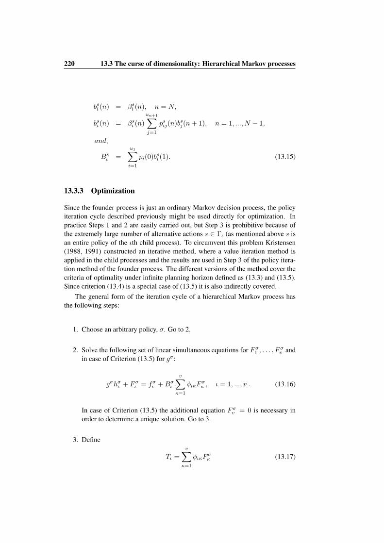
220 13.3 The curse of dimensionality: Hierarchical Markov processes
bsi (n) = βsi (n), n = N,
bsi (n) = βsi (n)
un+1∑j=1
psij(n)bsj(n+ 1), n = 1, ..., N − 1,
and,
Bsι =
u1∑i=1
pi(0)bsi (1). (13.15)
13.3.3 Optimization
Since the founder process is just an ordinary Markov decision process, the policyiteration cycle described previously might be used directly for optimization. Inpractice Steps 1 and 2 are easily carried out, but Step 3 is prohibitive because ofthe extremely large number of alternative actions s ∈ Γι (as mentioned above s isan entire policy of the ιth child process). To circumvent this problem Kristensen(1988, 1991) constructed an iterative method, where a value iteration method isapplied in the child processes and the results are used in Step 3 of the policy itera-tion method of the founder process. The different versions of the method cover thecriteria of optimality under infinite planning horizon defined as (13.3) and (13.5).Since criterion (13.4) is a special case of (13.5) it is also indirectly covered.
The general form of the iteration cycle of a hierarchical Markov process hasthe following steps:
1. Choose an arbitrary policy, σ. Go to 2.
2. Solve the following set of linear simultaneous equations for F σ1 , . . . , F
σv and
in case of Criterion (13.5) for gσ:
gσhσι + F σ
ι = fσι +Bσ
ι
v∑κ=1
φικFσκ , ι = 1, ..., v . (13.16)
In case of Criterion (13.5) the additional equation F σv = 0 is necessary in
order to determine a unique solution. Go to 3.
3. Define
Tι =v∑
κ=1
φικFσκ (13.17)

13.3 The curse of dimensionality: Hierarchical Markov processes 221
under Criterion (13.3) and Tι = 0 under Criterion (13.5). For each childprocess, ι, find by means of the recurrence equations
τι,i(n) = maxd
rdi (n)−md
i (n)gσ + βdi (N)Tι
, n = N
τι,i(n) = maxd
rdi (n)−md
i (n)gσ + βdi (n)
un+1∑j=1
pdij(n)τι,j(n+ 1)
,
n = 1, ..., N − 1 (13.18)
a policy s′ of the child process. The action s′(n) is equal to the d′ thatmaximizes the right hand side of the recurrence equation of state i at stagen. Put σ′(ι) = s′ for ι = 1, . . . , v. If σ′ = σ, then stop since an optimalpolicy is found. Otherwise, redefine σ according to the new policy (i.e. putσ = σ′ and go back to 2.
When the iteration cycle is used under Criterion (13.3) all physical outputs(md
i (n) and accordingly also hσι ) are put equal to zero. The iteration cycle covering
this situation was developed by Kristensen (1988).Under Criterion (13.4) all physical outputs, md
i (n), and all discount factorsβd
i (n) and Bσι are put equal to 1, but under Criterion (13.5) only the discount fac-
tors are put equal to 1. The iteration cycle covering these situations was describedby Kristensen (1991).
13.3.4 Discussion and applications
The hierarchical Markov process is specially designed to fit the structure of animaldecision problems where the successive stages of the child processes correspondto the age of the animal in question. By appropriate selection of state spaces in thechild processes and the founder process it is possible to find optimal solutions toeven very large models. The idea is to let the number of states in the child processes(where a value iteration technique is applied) be very large and only include veryfew states in the main process (where the technique is directly based on the policyiteration method). Thus we have got a method which is at the same time fast, exactand able to handle very large models.
Kristensen (1987) used the technique in a dairy cow replacement model whichin a traditional formulation as an ordinary Markov decision process would havecontained approximately 60,000 states, and later Kristensen (1989) in a model withapproximately 180 000 states. In both cases the number of states in the founderprocess was only 5, reducing Step 2 to the solution of only 5 simultaneous linearequations (versus 180,000 in a traditional formulation). Also Houben et al. (1994)used the method in a dairy cow replacement model. The reduction of the systemof equations was in their case from 6,821,724 to just 1, because no permanenttraits were considered in the model. An interesting aspect of their model is that for

222 13.3 The curse of dimensionality: Hierarchical Markov processes
the first time a disease is taken into account. Haran (1997) also built a dairy cowreplacement model based on a hierarchical Markov process.
In a different application area, Mourits et al. (1999) used a hierarchical Markovprocess in the determination of optimal feeding level and insemination age for dairyheifers. Similar ideas for use in fattening of bull calves have been presented byMakulska and Kristensen (1999).
In sows, Huirne et al. (1993) seem to have applied a technique which in manyaspects is similar to a hierarchical Markov process, but they have not explainedtheir method in all details. Also Jørgensen (1992) has applied a technique whichis inspired of a hierarchical Markov process in a sow replacement model, and later(Jørgensen, 1993), he used the hierarchical method in the determination of optimaldelivery policies in slaughter pigs. Also Broekmans (1992) used the method in thedetermination of optimal delivery policies in slaugther pigs taking random varia-tion in prices into account. More recent applications to slaughter pigs include Kure(1997) and, in particular, Toft et al. (2005) who studied the influence of epidemicdiseases on the slaughter policies. Verstegen et al. (1998) used the technique in anexperimental economics study investigating the utility value of management infor-mation systems. They used a formulation involving Bayesian updating of traits asdescribed by Kristensen (1993).
Naturally the hierarchical model just described may also be formulated as anordinary Markov decision process. In that case each combination of child process(founder state), stage and state should be interpreted as a state. We shall denote astate in the transformed process as (ιni), and the parameters are
rdιni = rd
i (n),md
ιni = mdi (n) ,
βdιni = βd
i (n), (13.19)
pd(ιni)(κmj) =
pd
ij(n), ι = κ ∧m = n− 1φικpi(0), n = N ∧m = 10, otherwise
,
where the parameters mentioned on the right hand side of the equations are thosebelonging to the ιth child process except for pi(0) which belongs to child processκ. This formulation of course has the same optimal policies as the hierarchical for-mulation, so it is only computational advantages that make the hierarchical modelrelevant. A comparison to traditional methods may therefore be relevant.
Since the policy iteration method involves the solution of a set of u equations(where u is the number of states) it is only relevant for small models. The valueiteration method, however, has been used with even very large models and mayhandle problems of the same size as the hierarchical formulation, but the time spendon optimization is much lower under the hierarchical formulation. To recognizethis, we shall compare the calculations involved.

13.3 The curse of dimensionality: Hierarchical Markov processes 223
Step 3 of the hierarchical optimization involves exactly the same number ofoperations as one iteration of the value iteration method (Eq. 13.6). The furtherneeds of the hierarchical method are the calculation of the rewards and either thephysical output or the expected discount factor of a stage in the founder processaccording to Eqs. (13.14) and (13.15). Since the calculations at each stage isonly carried out for one action, the calculation of both founder state parametersinvolves approximately the same number of operations as one iteration under thevalue iteration method if the number of alternative actions is 2. If the number ofactions is higher, the calculations relatively involves a lower number of operationsthan an iteration under the value iteration method. These considerations are basedon the assumption that the value iteration method is programmed in an efficientway, so that the sum of Eq. (13.6) is not calculated as a sum of all u elements,but only as a sum of those elements where pd
ij is not zero according to Eq. (13.19).Otherwise the hierarchical technique will be even more superior. Finally the systemof linear equations of Step 2 of the hierarchical cycle must be solved, but in largemodels with only a few states in the founder process the time spent on this isnegligible.
If we use the considerations above in a practical example, the advantages of thehierarchical technique becomes obvious. As reported by Kristensen (1991) a modelwith 180,000 state combinations was optimized by the hierarchical technique under100 different price conditions. The number of iterations needed ranged from 3to 6 corresponding to between 6 and 12 iterations of the value iteration method.If the latter method was used instead, a planning horizon of 20 years would berealistic (cf. van Arendonk, 1985). Since each state in the model equals 4 weeks,this horizon represents 260 iterations, which should be compared to the equivalenceof from 6 to 12 when the hierarchical technique was applied.
13.3.5 The numerical example formulated and solved as a hierarchi-cal Markov process
In order to illustrate the hierarchical technique, we shall formulate the numeri-cal example (the 36-state model) as a hierarchical Markov process. A Java basedsoftware tool for hierarchical Markov processes has been developed by Kristensen(2003)2. The following example is pre-defined and comes with the program.
The three classes of the genetic merit are defined as states in the founder pro-cess of a hierarchical Markov process. Thus the number of child processes is also3, and each child process represents a dairy cow of a certain genetic merit. Whena new heifer is purchased, we assume, like before, that the probability distributionover main states is uniform, so that the probability of entering either one is 1/3. Themaximum age of a cow was assumed to be 4 lactations, and the states of the childprocess are defined from the relative level of milk yield. Further a dummy state
2The program is available on World Wide Web. A Windows installer file may be downloadedfrom URL: http://www.prodstyr.ihh.kvl.dk/software/mlhmp.html

224 13.3 The curse of dimensionality: Hierarchical Markov processes
Table 13.11: Parameters of the hierarchical Markov process: Transition probabil-ities of founder process and initial state probabilities of child pro-cesses.
Transition probabilities, founder Initial state probabilities, childrenState φικ pi(0)ι κ=1 κ=2 κ=3 i = 1 i = 2 i = 3 i = 41 1/3 1/3 1/3 1/3 1/3 1/3 02 1/3 1/3 1/3 1/3 1/3 1/3 03 1/3 1/3 1/3 1/3 1/3 1/3 0
of length, reward and output equal to 0 is included at each stage of the child pro-cesses. If the cow is replaced at the end of a stage, the process enters the dummystate with probability 1 at the next stage, and for the rest of the duration of thesubprocess it will stay in the dummy states. Stage numbers in the child processesdirectly correspond to lactation numbers.
Thus, for all child processes, the probability of staying at the same relative levelof milk yield (state in the subprocess) is 0.6, and if the present state is “Average”,the probability of transition to either “Low” or “High” is 0.2 each. The probabilityof transition (if kept) from “Low” or “High” to “Average” is in both cases 0.3,and from “Low” to “High” and vice versa the probability is 0.1. The initial stateprobabilities of the child processes represent the probability of a new heifer beingeither “Low”, “Average” or “High” yielding. Thus, all initial state probabilities are1/3.
Like before, the physical outputs are interpreted as milk yields and the rewardsare defined as the economic net returns. All parameters of the hierarchical modelare shown in Tables 13.12 and 13.11.
We shall determine an optimal solution under the following 3 criteria of opti-mality:
1. Maximization of total expected discounted rewards, i.e., the objective func-tion (13.3). In this case the physical outputs of Table 13.12 are ignored, anda discount factor βd
i (n) = exp(−r), where r is the interest rate, is applied(for states where the stage length is not zero).
2. Maximization of average rewards over time. In this situation we use theobjective function (13.5) letting the output represent stage length. No dis-counting is performed in this case.
3. Maximization of average rewards over output defined as in Table 13.12.Thus the objective function (13.5) is applied, and no discounting is per-formed.
In Table 13.13, optimal policies under the three criteria are shown. It appearsthat the policies under the first two criteria are quite similar, but under the third

13.3 The curse of dimensionality: Hierarchical Markov processes 225
Table 13.12: Parameters of the hierarchical Markov process, child processes.p1
ij(n) p2ij(n)
ι n i j=1 j=2 j=3 j=4 r1i (n) m1
i (n) j=1 j=2 j=3 j=4 r2i (n) m2
i (n)1 1 1 0.6 0.3 0.1 0.0 6,000 3,000 0.0 0.0 0.0 1.0 5,000 3,0001 1 2 0.2 0.6 0.2 0.0 8,000 4,000 0.0 0.0 0.0 1.0 7,000 4,0001 1 3 0.1 0.3 0.6 0.0 10,000 5,000 0.0 0.0 0.0 1.0 9,000 5,0001 1 4 0.0 0.0 0.0 1.0 0 0 0.0 0.0 0.0 1.0 0 01 2 1 0.6 0.3 0.1 0.0 8,000 4,000 0.0 0.0 0.0 1.0 7,000 4,0001 2 2 0.2 0.6 0.2 0.0 10,000 5,000 0.0 0.0 0.0 1.0 9,000 5,0001 2 3 0.1 0.3 0.6 0.0 12,000 6,000 0.0 0.0 0.0 1.0 11,000 6,0001 2 4 0.0 0.0 0.0 1.0 0 0 0.0 0.0 0.0 1.0 0 01 3 1 0.6 0.3 0.1 0.0 8,000 4,000 0.0 0.0 0.0 1.0 7,000 4,0001 3 2 0.2 0.6 0.2 0.0 10,000 5,000 0.0 0.0 0.0 1.0 9,000 5,0001 3 3 0.1 0.3 0.6 0.0 12,000 6,000 0.0 0.0 0.0 1.0 11,000 6,0001 3 4 0.0 0.0 0.0 1.0 0 0 0.0 0.0 0.0 1.0 0 01 4 1 - - - - 6,000 3,500 - - - - 6,000 3,5001 4 2 - - - - 8,000 4,500 - - - - 8,000 4,5001 4 3 - - - - 10,000 5,500 - - - - 10,000 5,5001 4 4 - - - - 0 0 - - - - 0 02 1 1 0.6 0.3 0.1 0.0 8,000 4,000 0.0 0.0 0.0 1,0 7,000 4,0002 1 2 0.2 0.6 0.2 0.0 10,000 5,000 0.0 0.0 0.0 1.0 9,000 5,0002 1 3 0.1 0.3 0.6 0.0 12,000 6,000 0.0 0.0 0.0 1.0 11,000 6,0002 1 4 0.0 0.0 0.0 1.0 0 0 0.0 0.0 0.0 1.0 0 02 2 1 0.6 0.3 0.1 0.0 10,000 5,000 0.0 0.0 0.0 1.0 9,000 5,0002 2 2 0.2 0.6 0.2 0.0 12,000 6,000 0.0 0.0 0.0 1.0 11,000 6,0002 2 3 0.1 0.3 0.6 0.0 14,000 7,000 0.0 0.0 0.0 1.0 13,000 7,0002 2 4 0.0 0.0 0.0 1.0 0 0 0.0 0.0 0.0 1.0 0 02 3 1 0.6 0.3 0.1 0.0 10,000 5,000 0.0 0.0 0.0 1.0 9,000 5,0002 3 2 0.2 0.6 0.2 0.0 12,000 6,000 0.0 0.0 0.0 1.0 11,000 6,0002 3 3 0.1 0.3 0.6 0.0 14,000 7,000 0.0 0.0 0.0 1.0 13,000 7,0002 3 4 0.0 0.0 0.0 1.0 0 0 0.0 0.0 0.0 1.0 0 02 4 1 - - - - 8,000 4,500 - - - - 8,000 4,5002 4 2 - - - - 10,000 5,500 - - - - 10,000 5,5002 4 3 - - - - 12,000 6,500 - - - - 12,000 6,5002 4 4 - - - - 0 0 - - - - 0 03 1 1 0.6 0.3 0.1 0.0 10,000 5,000 0.0 0.0 0.0 1.0 9,000 5,0003 1 2 0.2 0.6 0.2 0.0 12,000 6,000 0.0 0.0 0.0 1.0 11,000 6,0003 1 3 0.1 0.3 0.6 0.0 14,000 7,000 0.0 0.0 0.0 1.0 13,000 7,0003 1 4 0.0 0.0 0.0 1.0 0 0 0.0 0.0 0.0 1.0 0 03 2 1 0.6 0.3 0.1 0.0 12,000 6,000 0.0 0.0 0.0 1.0 11,000 6,0003 2 2 0.2 0.6 0.2 0.0 14,000 7,000 0.0 0.0 0.0 1.0 13,000 7,0003 2 3 0.1 0.3 0.6 0.0 16,000 8,000 0.0 0.0 0.0 1.0 15,000 8,0003 2 4 0.0 0.0 0.0 1.0 0 0 0.0 0.0 0.0 1.0 0 03 3 1 0.6 0.3 0.1 0.0 12,000 6,000 0.0 0.0 0.0 1.0 11,000 6,0003 3 2 0.2 0.6 0.2 0.0 14,000 7,000 0.0 0.0 0.0 1.0 13,000 7,0003 3 3 0.1 0.3 0.6 0.0 16,000 8,000 0.0 0.0 0.0 1.0 15,000 8,0003 3 4 0.0 0.0 0.0 1.0 0 0 0.0 0.0 0.0 1.0 0 03 4 1 - - - - 10,000 5,500 - - - - 10,000 5,5003 4 2 - - - - 12,000 6,500 - - - - 12,000 6,5003 4 3 - - - - 14,000 7,500 - - - - 14,000 7,5003 4 4 - - - - 0 0 - - - - 0 0
Legends: ι = Child process (Founder State), n = Stage number, i = State at Stagen, j = State at Stage n+ 1.

226 13.3 The curse of dimensionality: Hierarchical Markov processes
Table 13.13: Optimal policies under the three criteria (c1, c2, c3) defined in thetext (actions: 1 = “Keep”, 2 = “Replace”).
State 1 State 2 State 3Subprocess Stage c1 c2 c3 c1 c2 c3 c1 c2 c3
1 1 2 2 1 2 2 1 2 1 11 2 2 2 1 2 2 1 2 1 11 3 2 2 1 2 2 1 2 2 12 1 1 1 1 1 1 1 1 1 12 2 2 1 1 1 1 1 1 1 12 3 2 2 1 2 1 1 1 1 13 1 1 1 1 1 1 1 1 1 13 2 1 1 1 1 1 1 1 1 13 3 1 1 1 1 1 1 1 1 1
Table 13.14: The performance of the hierarchical technique compared to the pol-icy and value iteration methods under the three criteria (c1, c2, c3)defined in the text.
Hierarchical model Policy iteration Value iterationc1 c2 c3 c1 c2 c3 c1 c2 c3
Number of iterations 4 3 2 4 4 2 100 100 100Computer time, rel. 1 0.86 0.43 268 267 139 48 46 11
criterion the optimal policy differs significantly. A more detailed example of theeffect of criterion of optimality was discussed by Kristensen (1991).
In order to compare the efficiency of the hierarchical technique to the tradi-tional policy and value iteration methods, the problem of the example was trans-formed to an ordinary Markov decision process and optimized by those methods.The transformed model has 3 × 4 × 4 = 48 states, which is not larger than thepolicy iteration method may be applied without problems. In Table 13.14 someperformance data of the three optimization techniques are compared.
The superiority of the hierarchical technique over the policy iteration method isdue mainly to the time spent on solving the linear simultaneous equations of Step2. In the hierarchical case a system of 3 equations is solved, whereas 48 equationsare solved under the ordinary policy iteration method.
In this numerical example the performance of the hierarchical technique is evenmore superior to the value iteration method than expected from the theoretical con-siderations of Section 13.3.4. In the present case an iteration of the hierarchicalmodel is performed even faster than one of the value iteration method applied tothe same (transformed) model. The reason is that the value iteration algorithm hasnot been programmed in the most efficient way as defined in Section 13.3.4. On thecontrary, the sum of Eq. (13.6) has been calculated over all 48 states of the trans-
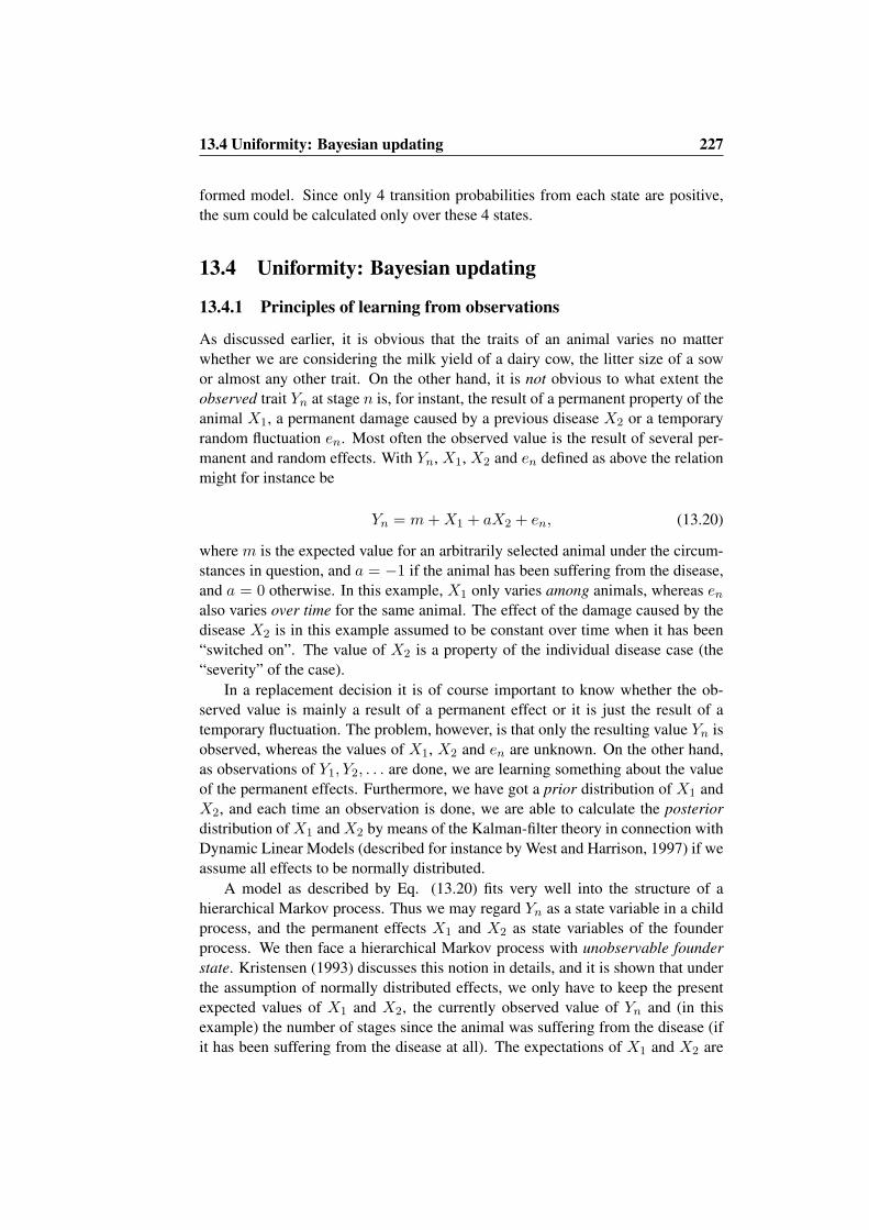
13.4 Uniformity: Bayesian updating 227
formed model. Since only 4 transition probabilities from each state are positive,the sum could be calculated only over these 4 states.
13.4 Uniformity: Bayesian updating
13.4.1 Principles of learning from observations
As discussed earlier, it is obvious that the traits of an animal varies no matterwhether we are considering the milk yield of a dairy cow, the litter size of a sowor almost any other trait. On the other hand, it is not obvious to what extent theobserved trait Yn at stage n is, for instant, the result of a permanent property of theanimal X1, a permanent damage caused by a previous disease X2 or a temporaryrandom fluctuation en. Most often the observed value is the result of several per-manent and random effects. With Yn, X1, X2 and en defined as above the relationmight for instance be
Yn = m+X1 + aX2 + en, (13.20)
where m is the expected value for an arbitrarily selected animal under the circum-stances in question, and a = −1 if the animal has been suffering from the disease,and a = 0 otherwise. In this example, X1 only varies among animals, whereas enalso varies over time for the same animal. The effect of the damage caused by thedisease X2 is in this example assumed to be constant over time when it has been“switched on”. The value of X2 is a property of the individual disease case (the“severity” of the case).
In a replacement decision it is of course important to know whether the ob-served value is mainly a result of a permanent effect or it is just the result of atemporary fluctuation. The problem, however, is that only the resulting value Yn isobserved, whereas the values of X1, X2 and en are unknown. On the other hand,as observations of Y1, Y2, . . . are done, we are learning something about the valueof the permanent effects. Furthermore, we have got a prior distribution of X1 andX2, and each time an observation is done, we are able to calculate the posteriordistribution of X1 and X2 by means of the Kalman-filter theory in connection withDynamic Linear Models (described for instance by West and Harrison, 1997) if weassume all effects to be normally distributed.
A model as described by Eq. (13.20) fits very well into the structure of ahierarchical Markov process. Thus we may regard Yn as a state variable in a childprocess, and the permanent effects X1 and X2 as state variables of the founderprocess. We then face a hierarchical Markov process with unobservable founderstate. Kristensen (1993) discusses this notion in details, and it is shown that underthe assumption of normally distributed effects, we only have to keep the presentexpected values of X1 and X2, the currently observed value of Yn and (in thisexample) the number of stages since the animal was suffering from the disease (ifit has been suffering from the disease at all). The expectations of X1 and X2 are

228 13.5 Herd restraints: Parameter iteration
sufficient to determine the current posterior distribution of the variables, becausethe variance is known in advance. Even though the posterior variance decreases asobservations are done, the decrease does not depend on the values of Y1, Y2, . . .,but only on the number of observations done.
In the study of Kristensen (1993), a more general case involving several traitseach being influenced by several unobservable effects is sketched, and a numericalexample involving only a single trait is given. An example concerning replacementof sows has been given by Jørgensen (1992). It was demonstrated in both studiesthat the Bayesian approach in some cases may result in state space reduction with-out loss of information. In multi-trait updating models a Kalman filter techniquemay be relevant as described by Kristensen (1994).
13.4.2 Applications
The described principles for Bayesian updating have in particular been used incombination with Dynamic Linear Models (see West and Harrison, 1997, for a de-tailed description of the concept). In addition to the model by Jørgensen (1992),such models with built-in learning capabilities have been developed by Kristensenand Søllested (2004a,b) for sow replacement taking all litter size results into ac-count. Lien et al. (2003) developed a model for determination of optimal lengthof leys in an area with winter damage problems, where the productivity of the leyis learned over time as observations are done. Finally, the principles are used in aslaughter pig marketing model with emphasis on information from online weighingequipment (Kristensen et al., 2006).
13.5 Herd restraints: Parameter iteration
One of the major difficulties identified in the introduction was herd restraints.All the replacement models mentioned in the previous sections have been single-component models, i.e., only one animal is considered at the same time, assumingan unlimited supply of all resources (heifers or gilts for replacement, feed, laboretc) and no production quota. In a multi-component model all animals of a herdare simultaneously considered for replacement. If all animals (components) com-pete for the same limited resource or quota, the replacement decision concerningan animal does not only depend on the state of that particular animal, but also onthe states of the other animals (components) of the herd.
If the only (or at least the most limiting) herd restraint is a limited housingcapacity, the number of animals in production is the scarce resource, and accord-ingly the relevant criterion of optimality is the maximization of net revenues peranimal as it is expressed in the criteria (13.1), (13.2), (13.3) and (13.4). Thusthe optimal replacement policy of the single component model is optimal for themulti-component model too.

13.5 Herd restraints: Parameter iteration 229
If the only (or most limiting) herd restraint is a milk quota, the situation is muchmore complicated. Since the most limiting restriction is a fixed amount of milk toproduce, the relevant criterion of optimality is now the maximization of average netrevenues per kg milk yield as expressed in criterion (13.5), because a policy thatmaximizes net revenues per kg milk will also maximize total net revenues from theherd which was assumed to be the objective of the farmer.
By following a policy which is optimal according to criterion (13.5) we assureat any time that the cows which produce milk in the cheapest way are kept. Thus theproblem of selecting which cows to keep in the long run (and the mutual rankingof cows) is solved, but the problem of determining the optimal number of cowsin production at any time is not solved. If for instance, it is recognized 2 monthsbefore the end of the quota year that the quota is expected to be exceeded by 10percent, we have to choose whether to reduce the herd size or to keep the cows andpay the penalty. The problem is that both decisions will influence the possibilitiesof meeting the quota of the next year in an optimal way. To solve this short runquota adjustment problem we need a true multi-component model.
An other example of a herd restraint is a limited supply of heifers. If thedairy farmer only uses home-grown heifers for replacement, the actions concern-ing individual cows become inter-dependent, and again a multi-component modelis needed in order to solve the replacement problem. Ben-Ari and Gal (1986)and later Kristensen (1992) demonstrated that the replacement problem in a dairyherd with cows and a limited supply of home grown heifers may be formulatedas a Markov decision process involving millions of states. This multi-componentmodel is based on a usual single-component Markov decision process represent-ing one cow and its future successors. Even though the hierarchical techniquehas made the solution of even very large models possible, such a model is far toolarge for optimization in practice. Therefore, the need for an approximate methodemerged, and a method called parameter iteration was introduced by Ben-Ari andGal (1986).
The basic idea of the method is to approximate either the present value func-tion fi(n) (objective function (13.3)) or the relative values fs
i (objective functions(13.4) and (13.5)) by a function G involving a set of parameters a1, . . . , am to bedetermined in such a way thatG(i, a1, . . . , am) ≈ fi(n) orG(i, a1, . . . , am) ≈ fs
i .In the implementation of Ben-Ari and Gal (1986) the parameters were deter-
mined by an iterative technique involving the solution of sets of simultaneous linearequations generated by simulation.
In a later implementation Kristensen (1992) determined the parameters by or-dinary least squares regression on a simulated data set. The basic idea of the im-plementation is to take advantage from the fact that we are able to determine anoptimal solution to the underlying (unrestricted) single-component model. If noherd restraint was present, the present value of the multi-component model wouldequal the sum of the present values of the individual animals determined from theunderlying single-component model. Then it is argued in what way the restraintwill logically reduce the (multi-component) present value, and a functional expres-

230 13.6 General discussion
sion having the desired properties is chosen. The parameters of the function areestimated from a simulated data set, and the optimal action for a given (multi-component) state is determined as the one that maximizes the corrected presentvalue. (A state in the multi-component model is defined from the states of theindividual animals in the single-component model, and an action defines the re-placement decision of each individual animal).
Ben-Ari and Gal (1986) compared the economic consequences of the resultingoptimal multi-component policy to a policy defined by dairy farmers, and theyshowed that the policy from the parameter iteration method was better. Kris-tensen (1992) compared the optimal multi-component policies to policies fromusual single-component models in extensive stochastic simulations and showedthat the multi-component policies were superior in situations with shortage ofheifers.
The parameter iteration method has been applied under a limited supply ofheifers. It seems to be realistic to expect, that the method and the basic principles ofKristensen (1992) may be used under other kinds of herd restraints as for instancethe short time adjustment to a milk quota as mentioned above.
13.6 General discussion
In Section 13.1, the main difficulties concerning animal production models wereidentified as variability in traits, cyclic production, uniformity (the traits are diffi-cult to define and measure) and herd restraints. We are now able to conclude thatthe difficulties of variability and the cyclic production are directly solved by theapplication of Markov decision programming, but when the variability of severaltraits are included we face a problem of dimensionality. The formulation of thenotion of a hierarchical Markov process contributed to the solution of the dimen-sionality problem, but did not solve it. The upper limit of number of states to beincluded has been raised considerably, but not eliminated.
This is for instance clearly illustrated when we formulate multi-component herdmodels in order to deal with herd restraints. In that case we still have to use approx-imate methods to determine an “optimal” replacement policy. On the other hand ithas been demonstrated by Kristensen (1992) that the parameter iteration methodapplied to a multi-component herd model (even though it is only approximate) isable to improve the total net revenue compared to the application of a usual single-component (animal) model in a situation with shortage of heifers. The parameteriteration method is an important contribution to the problem of determining opti-mal replacement policies under herd restraints.
In other situations with a limiting herd restraint it may be relevant to use analternative criterion of optimality maximizing average net revenue per unit of thelimiting factor. This method has been successfully applied in a situation with milkproduction under a limiting quota.

13.6 General discussion 231
Recent results have also contributed to the solution of the uniformity problem.The Bayesian updating technique described in Section 13.4 has turned out to be apromising approach, which has been applied to several problems in farm manage-ment. It might also be a solution to the problem of including animal health as atrait to be considered. As concerns other traits such as litter size or milk yield theBayesian approach may in some cases result in a reduction of the state space with-out loss of information (Jørgensen, 1992; Kristensen, 1993). Thus it contributesindirectly to the solution of the dimensionality problem.
New developments in the area of Markov decision programming for herd man-agement support includes the notion of multi-level hierarchical models, where ac-tions are defined at different levels with different time horizons. Thus the methodis able to optimize decisions with different time horizons simultaneously as de-scribed by Kristensen and Jørgensen (2000). A good example of this technique is amodel developed by Nielsen et al. (2004) for optimization of decisions concerningwinter feeding level, summer grazing strategy, start of fattening and slaughteringof organic steers.
Also the development of a standard tool (the Java based MLHMP softwareKristensen, 2003) for (multi-level hierarchical) Markov decision processes is con-sidered to be promising for construction of decision support models in the future.

232 13.6 General discussion

Chapter 14
Monte Carlo simulation
14.1 Introduction
The use of simulation techniques has a long and established tradition within animalproduction. Use of simulation models to understand herd management problemswas the theme of the influential book Systems Analysis in Agricultural Management(Dent and Anderson, 1971), and since then several simulation models have beenformulated within the different animal production systems. This chapter is not anattempt to review these previous efforts.
Decision making in animal production has long been seen as a game withouta conscious opponent (a game against nature), and use of the Bayesian decisionstrategy of maximum expected utility has been the accepted criterion for choos-ing between the available actions. The underlying principle of acting based onthe prior (subjective) probability distribution of the state of nature is an importantpart of the framework. This is the foundation of the so-called Bayesian statisticalmethods. The use of Bayesian methods within statistics has been rather sporadicuntil recently. A reason for this is a philosophical debate concerning the existenceof subjective probabilities, especially whether it is acceptable to use subjectiveprobabilities in the analysis of experiments. Another reason, is the computationalcomplexity that is inherent in the Bayesian methods. This complexity barrier hasto a large degree been broken down, because of numeric techniques, and the useof Bayesian networks to exploit the independencies between elements within thesystem. Because of this, Bayesian methodology is currently a very active researcharea within statistics.
The systems approach used in simulation modeling has many things in com-mon with Bayesian modeling, and to the authors’ opinion, the reason researchersuse the modeling technique is an inherent wish to express their prior knowledge ofthe quantitative and qualitative structure of the system they investigate. This priorknowledge is based on results from many different experiments, observations inpractice, and scientific theory building. Bayesian methodology offers the theoreti-

234 14.2 The simulation method
cal framework for this specification. In addition it offers a more stringent approachto parameter estimation and model testing than the traditional systems approach.
This note is an attempt to describe, how this framework can be used within thesystems approach.
14.2 The simulation method
In Section 9.7 we have already given a rather detailed definition of the simulationmethod. The reader is encouraged to read that section again, before continuingwith this chapter, which only covers the Monte Carlo technique. Here, we shallonly give a very short summary for reference purpose.
A Monte Carlo simulation model is described by a set of parameters Φ =(Φ0,Φs•), where Φ0 represents the state of nature specified initially before thesimulation, and Φs• = (Φs1,Φs2, . . . ,Φst, . . . ,ΦsT ) represents parameters thatchange values during simulations (often called state variables. Further conceptsinclude the decision rule, Θ, and a set of output parameters Ω (typically a subset ofΦs•).
As defined in Section 9.7, the purpose of a Monte Carlo simulation modeldescribed by the parameters Φ = (Φ0,Φs•) is to calculate the expected utility,U(Θ), under a given decision rule, Θ, i.e.,
U(Θ) =∫ ∞
−∞U(Θ, φ)fΦ(φ)dφ (14.1)
=∫ ∞
−∞
∫ ∞
−∞U(Θ,Φs• | Φ0 = φ0)f(Φs•|Φ0)(φs• | φ0)fΦ0(φ0) dφs•dφ0,
where U is the utility function, which in general can refer to any function of theoutput variables. The functions fΦ, f(Φs•|Φ0) and fΦ0 are the density functions ofΦ, (Φs•|Φ0) and Φ0, respectively.
The Monte Carlo simulation technique is a numerical method for solving thisintegral. It relies on the drawing of random numbers. Every time the model en-counters a stochastic variable, a (pseudo)-random variable is drawn from the ap-propriate distribution and this value is used in the subsequent calculations. Eachcompleted calculation (simulation run) with the model represents a random draw-ing from the simultaneous distribution of input and output variables. By increasingthe number of calculations the distribution of the output variables can be specifiedto any degree of precision. The expected utility is found from:
U(Θ) ≈ 1k
k∑i=1
U(Θ, φi). (14.2)
where φi is a random drawing from the multidimensional distribution of the pa-rameters, and k is the number of random drawings (simulation runs).

14.2 The simulation method 235
14.2.1 Systems approach
Standard statistical methods for analysis of data, e.g. from experiments help infinding a sufficient model for the data. A sufficient model is such that the deviationfrom the model is random and independent from any known sources. Such a modelwill usually have very few parameters. In model comparisons between models withdifferent number of parameters, the model with fewest parameters is preferred, ifthere is no substantial evidence for the model with most parameters. This approachcan be justified for several reasons, from the practical experience that models withfew parameters are more robust, when applied to other data sources; from the Tay-lor expansion that approximates any function to a desired accuracy with a (loworder) polynomial; and, from the difficulty of separating effects of different pa-rameters if no prior knowledge of the parameters exists.
Usually each set of data is treated separately from previous experience. Incontrast, the simulation research method uses the systems approach, where existingknowledge of a system is build into the model.
The primary consideration within the system approach is the understanding ofa whole system. A system can e.g. be defined as in Clausen (1969).
A system is a part of reality that in some manner is detached (seemsdifferent) from the rest of reality. This rest is the environment ofthe system. Evidently the rest is also a system. These two systems(the system and its environment) are characterized by their individ-ual structure. But they are also interdependent. There is said to be acommunication between them.
Such a system cannot be understood by focusing on single elements of thesystem, the interaction and structure of the elements is just as important.
The modeling steps can be divided into several steps, e.g. definition of themodeling goals, system analysis, system synthesis, verification, validation and in-ference. The goal of the simulation model can be to develop a decision supportsystem or to integrate current knowledge concerning the system to enhance theunderstanding of the system etc. In the system analysis step the components, inter-actions, relationship and dynamic behavior of the system is isolated. The behaviorof each element is described using information from different sources, e.g. researchreports, new experiments. The object oriented approach is one of the techniquesthat can be used. In the system synthesis step the model is developed and pro-grammed according to the specifications in the system analysis step. The Objectoriented method makes it possible to make the structure and elements of the pro-gram closely correspond to the real system. Verification is the check of whether themodel behaves according to the system specification. Validation is the step wherethe model output is compared to data from the real world, and finally the inferencestep, where the model is used according to the goal. These steps are performedcyclically with subsequent refinement of model until the final model can be usedfor inference.
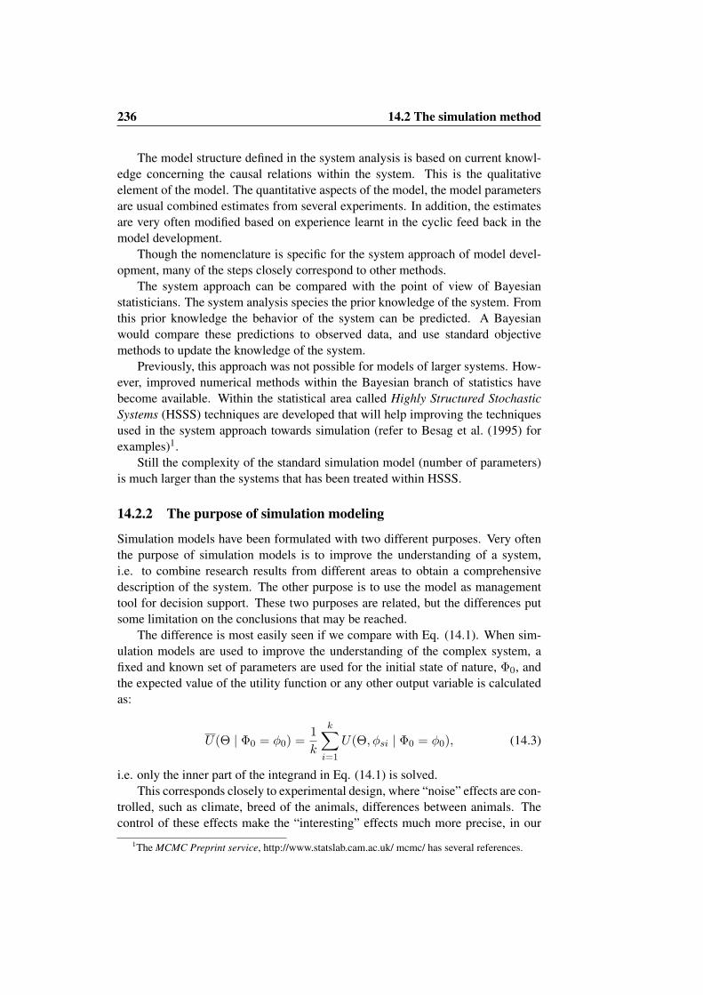
236 14.2 The simulation method
The model structure defined in the system analysis is based on current knowl-edge concerning the causal relations within the system. This is the qualitativeelement of the model. The quantitative aspects of the model, the model parametersare usual combined estimates from several experiments. In addition, the estimatesare very often modified based on experience learnt in the cyclic feed back in themodel development.
Though the nomenclature is specific for the system approach of model devel-opment, many of the steps closely correspond to other methods.
The system approach can be compared with the point of view of Bayesianstatisticians. The system analysis species the prior knowledge of the system. Fromthis prior knowledge the behavior of the system can be predicted. A Bayesianwould compare these predictions to observed data, and use standard objectivemethods to update the knowledge of the system.
Previously, this approach was not possible for models of larger systems. How-ever, improved numerical methods within the Bayesian branch of statistics havebecome available. Within the statistical area called Highly Structured StochasticSystems (HSSS) techniques are developed that will help improving the techniquesused in the system approach towards simulation (refer to Besag et al. (1995) forexamples)1.
Still the complexity of the standard simulation model (number of parameters)is much larger than the systems that has been treated within HSSS.
14.2.2 The purpose of simulation modeling
Simulation models have been formulated with two different purposes. Very oftenthe purpose of simulation models is to improve the understanding of a system,i.e. to combine research results from different areas to obtain a comprehensivedescription of the system. The other purpose is to use the model as managementtool for decision support. These two purposes are related, but the differences putsome limitation on the conclusions that may be reached.
The difference is most easily seen if we compare with Eq. (14.1). When sim-ulation models are used to improve the understanding of the complex system, afixed and known set of parameters are used for the initial state of nature, Φ0, andthe expected value of the utility function or any other output variable is calculatedas:
U(Θ | Φ0 = φ0) =1k
k∑i=1
U(Θ, φsi | Φ0 = φ0), (14.3)
i.e. only the inner part of the integrand in Eq. (14.1) is solved.This corresponds closely to experimental design, where “noise” effects are con-
trolled, such as climate, breed of the animals, differences between animals. Thecontrol of these effects make the “interesting” effects much more precise, in our
1The MCMC Preprint service, http://www.statslab.cam.ac.uk/ mcmc/ has several references.
14.2 The simulation method 237
case we need fewer simulation runs or in the experimental case, we need feweranimals.
Typical investigations under this framework, are sensitivity analyses, where theeffect of small changes in the parameters in Φ0. In this manner important param-eters can be isolated and research efforts directed towards a better understandingof these parameters. The knowledge of the systems sensitivity to changes in theparameters is part of, what we call understanding of a system.
In contrast, when simulation models are used to determine “optimal” strategieswe want to find the optimal set of decision rules given the precision in our currentknowledge of the parameters (state of nature). The parameters used in each simu-lation run should therefore be a sample from the prior distribution of Φ0 reflectingthe precision in our current knowledge, and not fixed values.
14.2.3 Dimensionality of simulation modeling
The dimensionality of a simulation model is the number of parameters that servesas input to the model.
The dimensionality is best understood when Eq. (14.1) is considered. It can besplit into three parts.
The dimensionality of state of nature : This is the number of parameters in Φ0
specifying the initial conditions. Typically this number is comparatively“small” (less than 100 different variables). Many of the parameters haveindependent prior distributions, reducing the problem of specifying the co-variance between the parameters. These parameters can often be estimatedusing Bayesian techniques. The dimensionality of the state of nature can becompared to the dimensionality of e.g. Markov chain probabilistic simula-tion approaches. Other numerical integration methods may be consideredfor the outer part of the integrand in Eq. (14.1)
The dimensionality of the systems’ state space : The number of parameters inΦs•. This will typically be very large, as each element in the simulationmodel and the interactions between the elements are represented. That is,the integration of the inner part of Eq. (14.1) is only tractable with the MonteCarlo simulation model.
The dimensionality of the decision space : Nothing general can be said of thisdimension. With simple heuristic rules the dimension may be very low, andwith complex models the dimensionality may approach the dimensionalityof the system state space. If the set of decision rules are too complicated, thesearch for optimality will usually be intractable.
The major problem with too many parameters in the model is that it is notpossible to distinguish effects of the different parameters based on observations.I.e. estimation, or learning, of the values of the parameters will result in verystrong dependency between the parameter estimates.
238 14.3 Why use the Monte Carlo Approach
14.3 Why use the Monte Carlo Approach
Within animal production several simulation models exist. These models are eitherdeterministic or probabilistic e.g. Markov Chain or Monte Carlo. Because of theflexibility of the latter approach, the method as such does not lead to any fixedset of assumptions. The assumptions differ from model to model. The two othermethods have some assumptions implied. These assumptions are not always statedin the model. Therefore, some of the consequences of the assumptions will bereviewed briefly.
14.3.1 The Deterministic Approach
The assumptions are of course that the real system has no stochastic variation. Inorder to understand the effect of the assumption, we can approximate the utilityfunction or any output variable by a second order Taylor expansion around thevalue Φ,
U(Φ) ≈ U(Φ) + U ′(Φ− Φ) +12(Φ− Φ)>U ′′(Φ− Φ), (14.4)
where U ′ is the vector of first derivatives of U() with respect to the parameters,and U ′′ is the matrix of second derivatives of U() with respect to the parameters.
The expectation and variance of this expression can in general not be founddirectly, but if we assume multivariate normal distribution of the parameters, wehave:
E(U(Φ)) ≈ U(Φ) +12tr(U ′′Var(Φ)) (14.5)
Var(U(Φ)) ≈ U ′Var(Φ)U ′> +12tr(U ′′Var(Φ))2 (14.6)
The major problem with deterministic models is the term that depends on the vari-ance in Eq. (14.5). This term only vanishes if U ′′ = 0, i.e. if U() is linear in theparameters or if Var(Φ) = 0. Neither case is likely to happen.
The problem with the deterministic models is not so much, that the variance onthe output is ignored, but that the calculated expectation is systematically wrong.Results from a deterministic model will not be correct even if all causal relationsand expectations of parameter values are correct. The value of such models isof course dubious, and knowledge of the magnitude of the systematic error is ofextreme importance, i.e. the second term in Eq. (14.5).
Probably (hopefully!) the severity of these problems does not interfere withthe use of deterministic models to understand causal relations in order to formulateresearch hypothesis.
14.3.2 The Markov chain approach
The Markov Chain approach is usually used for finding the steady state distribution,i.e. the expected long term probability of being in each of the states. As the states

14.3 Why use the Monte Carlo Approach 239
0 1 2 3 4 5 6 7 8 9 10 11 12 13 14 15 16 17 18 19 200.00
0.02
0.04
0.06
0.08
0.10
0.12
0.14
0.16
Number of farrowings
Probability
Figure 14.1: Probability distribution of number of animals in the farrowing statewhen steady state is reached in a Markov Chain simulation modelwith a herd size of 200 sows
are defined for an individual, the probability refers to a single individual. Thewhole herd can be studied if independency of the individuals is assumed.
Within the whole herd problem, we are interested in the distribution of howmany animals that are in each of the states. This can also be found from the steadystate distribution, even though usually only the steady state probability and the ex-pected number are reported. The distribution is multinomial with the total numberof animals and the steady state probabilities as parameters.
An example will illustrate this. In a sow herd model based on a step length of 1week, the steady state distributions shows that approximately 4 % of the sows willbe in the farrowing state. In a sow herd of 200 sows the probability distribution ofsows in this state is shown in Figure 14.1.
We can assign income (utility) to this curve. The income will increase linearlywith number of farrowings per week until the number of available pens is reached.If the number of farrowings is above the number of available pens, the incomewill most likely have a progressively lower slope, as the number of surplus sowsincreases, because there are not enough pens. Due to this non-linearity we cannotuse the expected probability to calculate the income, but must take the expectationfor each of the possible number of farrowings. On the other hand, such a directapplication of the income curve to the probability distributions will not sufficeeither. The problem is that the capacity restrictions will make the farmer react in

240 14.4 An object oriented model of a pig herd
case of surplus. This means that the probabilities used in the Markov Chain modelare not correct, because they do not only depend on the state of the animal but alsoon the state of the other animals. The remedy to this problem within the MarkovChain approach is to increase the state space to include the states of all the animalssimultaneously. This will make the problem grow prohibitively large, i.e. we areconfronted with the curse of dimensionality as discussed in Chapter 13.
Though the Markov Chain approach enables us to obtain the full probabilitydistribution, we still have the problem that this probability distribution is only cor-rect, if the animals are independent of each other. If capacity restrictions etc. existthis is not so.
14.3.3 Conclusion
The two simulation approaches have their limitation because of the implied as-sumptions of the methods.
Monte Carlo simulation offers a flexible approach for solving these inherentproblems. Of course, Monte Carlo simulation has other limitations, such as com-putation time and lack of a robust search strategy for optimality. Optimally, MonteCarlo simulation should be used to supplement other probabilistic approaches suchas Markov Chain or Bayesian Networks.
14.4 An object oriented model of a pig herd
To illustrate the modeling process, a description of a research project with an ob-ject oriented simulation model of a pig herd is presented in the following. Thedescription should mainly serve as an illustration of the object oriented concept. Itis based on Jørgensen and Kristensen (1995).
As in other simulation models the herd is described consisting of the animal,and its biological states, as well as the housing system, the confinement. The restof the production system plays a major role, i.e. the observation, the updatingand filtering of information, decision support systems, the decisions and the corre-sponding actions that are carried out. An outline of the production system is shownin Figure 14.2.
The system, a pig herd, is not stable, and rely on the manager’s continuouscorrection of the production flow. The manager uses his knowledge or belief inthe state of the herd. This belief is based on observations with varying precisionof the herd, e.g. observations of weight of the individual animal. The state ismeasured using a measuring device with given precision. The resulting observationis sent to a Belief Management System (BMS) that handles updating and filteringof the observation. The result is a belief in the state. This belief can be used in adecision support system (DSS). The output from the DSS is a suggested decision.The Manager then makes the final decision based on the information from theDSS. Finally the decision is turned into an action by the staff in the herd. Actions

14.4 An object oriented model of a pig herd 241
observations
belief
suggested decisions
decisions
actions
DSS
manager
worker
BMS
Confinement
Animals
Mating
Weaning Farrowing
Introduction
Culling
Figure 14.2: The elements of a pig production herd
comprise e.g. matings, weanings, movements, and observations. The objects in themodel communicate by a message passing scheme that also handles the dynamicupdating of the model.
14.4.1 General layout
The simulation model is programmed in Borland Pascal 7.0 as a program to be rununder Windows. The program has two basic classes: DinaPigObjects and Mes-sages sent between two DinaPigObjects. A message consists mainly of a messagetime, a Receiver and Sender ID, a command and the strength of the command. Sim-ilarly the main features of a DinaPigObject are an ID and a method for handlingMessages. The main structure in the program is a sorted list or queue of Messages,sorted according to message time. The simulation is carried out by retrieving thefirst Message in the queue. The system time is updated to the message time. Thereceiver of the message (a DinaPigObject) is asked to handle the message. Themessage is then deleted and the next message in the queue is processed. The han-dling of the message will typically produce additional messages to other objects,as well as to the receiver itself. The scheduling of the simulation model is handledby the message processing. The posting of a message from the receiver to itselfwith a time lag allows for adjustment of the updating frequency of the model. Thefirst step in the handling of messages by a DinaPigObject is an updating from theprevious to the current system time. The scheduling method is thus a modification

242 14.4 An object oriented model of a pig herd
of the event-driven method, where additional events are generated with fixed timeintervals, but the updating may occur with varying time steps.
This comparatively simple structure can handle the full complexity of the sim-ulation model.
Seven main descendants of the DinaPigObject have been defined, i.e. the ani-mals, the physiological states of the animals, the confinement, the manager and thestaff, the measuring device, the belief management system and the decision sup-port system. These will be described in the following. Different descendants ofthe Message class are used to handle the observations, the beliefs, the suggesteddecision, decisions and actions.
14.4.2 Modeling the confinement
Objects with relation to the confinement are based on a class that inherits the fea-tures of DinaPigObject but in addition has three lists assigned. A list of pointsdefining the outline of the confinement, a list of resources, e.g. drinking nipples,feeders, and an item list of other items. The main descendants of this class are De-partments, Sections and Pens. The item list of a department consists of Sections.The item list of a section consists of pens and the item list of a pen consists ofanimals.
14.4.3 Modeling the animal and its physiological states
The model of the animal itself is very simple, as the detailed model is handled in thedescription of the different physiological states of the animal. An animal simplyhas a list of states assigned and a list of internal messages between the states of theanimal. The message handling starts with an updating of each state in the state listto the current simulation time.
State description
Each animal has a list of state’s assigned. Each state models a physiological pro-cess. As mentioned the states are assigned an animal. Each state has a transitionfunction that updates the previous physiological state to the state at the currenttime. In addition some states are observable and some states can be influenced byoutside events. Current states are growth process, death-process, generic diseaseprocess, puberty, oestrus, pregnancy and lactation.
14.4.4 Modeling the measuring device
The modeling of the physiological state of the animal relies, as shown above, ondetailed models and a number of parameters. This is in order to get as close aspossible an approximation to the real, biological system.
This detailed knowledge of the biological systems is in general not available atthe herd level. Instead, the pig producers have to rely on observations in the herd.

14.4 An object oriented model of a pig herd 243
It is important to make this distinction in the model. Therefore, all information tothe pig producer has to be based on observations. To represent this in the modelthe concept of a measuring device is used. The concept covers both actual devices,e.g. weighing scales, pregnancy testers, as well as virtual devices, e.g. assessmentof the health state or weight of an animal by eye.
In the model the manager sends a message to the measuring device in order toobtain an observation on an animal. The measuring device in turn sends a messageto the animal and the animal returns a message with the requested value in thestrength parameter of the message. The measuring device transforms the strengthand returns the value to the manager.
The simplest measuring device is a device for making quantitative measure-ments. It simply adds a random noise to the value received from the animal. Themeasurement device is thus defined with a measurement precision (i.e. the recip-rocal of the variance of the random noise). Another class of measuring devices isused for categorical measurements, e.g. pregnancy testing, heat detection, diseasediagnose. These devices return a measurement such as pregnant/not pregnant, dis-eased/healthy. These measurements are prone to mistakes, just as the quantitativemeasurements. The definition of these devices relies on the concept of an under-lying continuous distribution with threshold values to define the intervals for thedifferent categories. The strength returned from the animal is added a random noise(with a given precision) and subsequently categorized according to the thresholdvalues. In this manner different precision and sensitivity can be modeled. E.g. thedisease state of the animal described above will return a 0 if the animal is healthyand 1 if the animal is infected. This value is added a random value and the animalis classified as diseased if the resulting value is above e.g. 0.75.
14.4.5 Modeling the belief management system
The observations made should be used for adjusting the pig producers belief in thestate of his herd. In order to represent this in the model the concept of a BeliefManagement System is introduced. This is a general framework that should coversimple systems that e.g. calculate monthly averages of the production trait as wellas complicated Bayesian Networks that uses Bayesian methods for a correct han-dling of the observation. (The term BMS is inspired by the terminology used inrelation to causal or Bayesian Networks, e.g. Jensen, 1996, 2001). Ideally, eventhe subjective processing of information in the mind of the pig producer should becovered by this concept. However, our work has not yet carried us that far.
The “ideal” Belief Management System should simply use every measurementin the herd in order to estimate the parameters of the detailed biological mod-els using advanced statistical methods. The contrast between this ideal and themethod used in the real world, by pig producers as well as researchers, is strik-ing. Most management information systems rely on rather simple techniques, suchas quarterly or monthly averages of key production traits (cf. Chapter 5). A fewincorporate methods from production control such as CUSUM-charts. Recently,

244 14.4 An object oriented model of a pig herd
more advanced techniques have been applied, such as Kalman filtering techniques.These techniques combined with the techniques of Bayesian nets are promisingcandidates for the future BMS. Even though these techniques can solve very com-plex problems, the size of the problems will still set an upper limit to what can besolved. So, a BMS will have to rely on an approximation. It is important to realizethat a more complex system is not necessarily better from an economic point ofview, if the cost of obtaining the information is included.
It is not the intention to program the BMS directly in the simulation model.Instead, the simulation model communicates through a standard interface with theBMS. The observations from the model are transformed into beliefs. When themanager or DSS needs information concerning beliefs, they will send a messagewith a request. The BMS returns the belief.
The belief itself can be represented with varying simplicity. If the BMS onlycalculates monthly averages, it would be natural to let the belief in the production ofan animal be the monthly average. More advanced BMS would use the predictionof the future monthly average based in the historical data. The belief may even bebased on the individual animals own performance, and may include the variance aswell as the expectation.
Clearly, some representation of beliefs would be better than others, but thiswould be seen as a result (i.e. poorer production due to worse decisions), ratherthan as a defined standard for the BMS. This ensures that every method of dataprocessing can be described as a BMS.
Some of the aspects of a BMS are currently handled in the DSS, especiallyin those based on Markov Chain methodology. From a conceptual point of view,the distinction between BMS and DSS has proved to be valuable. In any casemany information systems exist that would be categorized as BMS without anyDSS element in it. Similarly many DSS exist with no calibration to the actualregistrations in the herd.
14.4.6 Modeling the decision support system
The DSS in the simulation model is not intended to be programmed directly intothe model, at least not for the more complicated models. Instead interface betweenDSS and the simulation model is established. The DSS can be of varying com-plexity including simple ’rules of thumb’ as well as complicated systems, such asthose based on Markov decision programming. Some of these DSS have includedelements that in our terminology would be called BMS. This is, however, only aproblem from a more formalistic point of view.
The DSS responds to messages from the Manager requesting suggested choiceof actions. A well-established problem solved by the DSS is the selection betweenthe actions cull the animal or keep the animal. Other important operational ac-tions are buying and selling of animals, movement of animals (weaning - regroup-ing etc), mating (actual decision ’refrain’ from mating sows in heat), induction ofevents, influence nutritional status/growth/meat quality through feeding, observe,

14.5 Representing model dynamics 245
timing of actions. Many of these actions are not currently covered by DSS but arehandled by heuristics. The heuristic rules will often differ between herds and theeconomic basis of the rules is not always adequate.
The DSS will usually base its suggested decision on the belief in the herd.Therefore, the BMS and DSS will often be tightly connected
14.4.7 Modeling the manager and the staff
From the start of project, the role intended for the manager in the simulation modelwas to transform suggested decisions from the DSS into actual decisions. Thistransformation should be based on e.g. different objectives, additional informationnot included in the DSS, constraints unknown to the DSS, and a possible irrationalcomponent.
An example of such a transformation is that the DSS suggest that the farmershould cull sow no. 101. The farmer decides to keep the sow. Possible reasonscould be that he will wait and see, if there is a replacement gilt coming in heat atthe right time, that the sow is easy to manage, that one of the other sows in thegroup has a sore leg and he wants to have a surplus “just in case”, that the sow isthe only one remaining from the foundation of the herd or that the piglets have a“cute” coloring. From the pig producers point of view all these reasons are validand should be taken into account although they are not included in the DSS.
This original role has still been kept, but some of the roles originally placed inthe DSS and BMS are still modeled as part the manager. This corresponds to therole played by the manager in previous simulation models, where the managementwere mainly described as a set of heuristic rules.
The work with the model has shown it of value to define experts, managementtasks and management schedules in order to structure the program. The experts aredescendants of the manager class and handle a subset of the management function,e.g. buying and selling of animals, weighing of animals, mating of animals. Tasksare mainly lists of linked actions, i.e. the movement of the pigs from one pen toanother involves several actions, e.g. find a section with empty pens, select the bestpen, move the pigs from the old pen etc. Typically the task sends a message to otherobjects and then waits for the responding messages before continuing. A scheduleis a description of tasks to be performed with regular intervals, e.g. weekly ormonthly.
14.5 Representing model dynamics
The dynamic systems that are modeled do of course evolve in continuous time. Inorder to simulate the system on the digital computer, we have to make a decision,how to represent the continuous time scale on the computer.

246 14.5 Representing model dynamics
14.5.1 Selection and effect of stepping method
First of all, a variable called system time is defined.Within animal simulation the most frequent approach is the fixed-time incre-
menting procedure. Using this procedure, first the system time is advanced withone unit. Then each element in the model is updated to this time, by determiningthe events that has happened, and the changes in the state variables. This procedureis in close accordance with the formulation of the models with difference equationsand discrete time Markov Chains.
Another approach next-event incrementing that is the most important in simu-lation of event driven systems (e.g. queuing systems). With this method the systemclock is incremented by a variable amount. Each time an element of the systemis updated, the time of the next event for that element is calculated (and elementsinfluenced by it). These future events are then stored in a sorted list. The next-eventincrementing simple sets the system clock to the time of the first element in the list,updates this element (and generates new events for the element) and continues withthe next element on the list.
Each approach has its advantages. Continuous growth processes will be diffi-cult to represent by the next event approach, while the handling of almost simulta-neous events is difficult in the fixed time approach. If only the first three animalsin oestrus should be mated, how do we decide which of the animals, it was, whenthey in principles show heat simultaneously.
Of course the methods can be combined, a simple approach is to include anartificial event with fixed time steps for each element in the model. The elementswill then be updated at least as frequent as the length of these time steps. This isthe approach used in the pig simulation model in the previous section.
The choice of the length of each time step in the fixed time incrementing ap-proach is another important decision to make in simulation models. Formally theoutput of the simulation model should not depend on our choice of time stepping.If the simulation should claim to represent the real system, a choice of calculationmethod should obviously have no influence. Very often the initial specification ofthe model does not allow changes in time step length. Therefore before we proceedwe will look on the two possible specification methods.
14.5.2 Difference equations
Let us describe a simple growth model.The animal is given an amount of feed, ∆FU , on a given day. This daily feed
intake is split into feed used for maintenance and feed used for growth.
∆FUmaintenance = kmaintenanceW0.75 (14.7)
∆FUgrowth = ∆FU −∆FUmaintenance + εfg (14.8)
The random term εfg is included in order to model the stochastic element in themodel.

14.5 Representing model dynamics 247
The growth can then be calculated:
∆W = kefficiency∆FUgrowth + εg
And the weight and total feed summarised
FUt+1 = FUt + ∆FUt (14.9)
Wt+1 = Wt + ∆W (14.10)
These so-called state variables are then kept until the next period.The stochastic elements are often assumed to be distributed independently and
N (0, σ2ε) (A different variance for each residual).
This is the difference equation approach and it seems to be the standard formu-lation of models within animal production.
Note that the length of the time step (1 day) is not formulated explicitly. Byselecting this time step in the model description, we are stuck with it. If we want tochange the length of the time steps in the model the formulas must be reformulated.If we take the weekly allowance of feed and base the calculation on that, we get adifferent answer than by applying the formula seven times in succession. As theanimal grows, the metabolic weight changes and this results in a lower daily gain.The time step one day seems “natural”, but we may be interested in making shortertime steps, in fact the feeding of animals is seldom an event that only occurs oncea day. Again the equations that we would have to use would be different (eventhough the difference would be smaller).
14.5.3 Differential equations
To avoid this, the model can be quantified on a continuous time scale as differentialequations.
The rate of feed energy used for maintenance and the rate of feed energy usedfor growth.
dFUmaintenance
dt= kmaintenanceW
0.75 (14.11)
dFUgrowth
dt=dFU
dt− dFUmaintenance
dt+ εfg (14.12)
The growth rate can then be calculateddW
dt= kefficiency
dFUgrowth
dt+ εg
We also have to specify an equation for the rate of feed available. The simplestcase is that the feed is available at a constant rate.
dFU
dt= kfeed
The weight and total feed consumption can then be found, as a solution to thedifferential equations.
The random terms in the model are normally assumed to follow the so-calledWiener process.

248 14.5 Representing model dynamics
Solution of the equations
Even though the formulas in the difference equations and the differential equationslook alike, it should be emphasized, they are not the same. However, in generalsuch differential equations have to be solved by numerical methods, and one ofthese methods, Euler’s method, uses the difference equations as approximations.It is important to recognize that Euler’s method is an inefficient method for solv-ing differential equations, and other far more precise and fast methods exist. Oneof these, the Runge-Kutta method, should be easy to implement in any simulationmodel. Other methods use a variable time stepping approach, i.e. the length ofthe time step is varied, until the difference in the function between the two timestep is sufficiently small. See any textbook on solving ordinary differential equa-tions for reference (e.g. Press et al., 1989). The Wiener process in continuous timecorresponds to the Normal distribution in fixed time interval. Further treatment ofthis process can be found in textbooks concerning Stochastic processes (e.g. Hoelet al., 1972).
Because of the interaction between model elements, the variable time stepmethod can be difficult to use in a herd simulation model. But a good idea isto compare model outputs with time steps of different length, to choose the methodthat results in the best trade off between computing time and accuracy. To be hon-est, very few simulation models within animal production have been through suchscrutiny, at least none has been published to our knowledge. The usual time step iseither one day or one week.
14.5.4 State transitions in continuous time
A similar discussion, as the one made above, can be made for the modeling of statetransitions. Markov chains cover both discrete and continuous time.
The Markov property is that if we know the current state, the future is inde-pendent of the past. In Markov chain models this property is ensured by defininga large discrete state space. The transition probability from the state thus only de-pends on the state, and not on the history. In Monte Carlo simulations models wedo not have this property, instead the state space is defined by a mixture of con-tinuous and discrete variables, as well as discrete states. Naturally these variableswill interact. The changes in the continuous variables will depend on the discretevariables, and vice versa.
It is often convenient to represent the transition from state to state in continuoustime by the intensity of transition. The intensity of transition is defined as
h(t) =f(t)
1− F (t)
The function h(t) is also called the hazard rate. h(t) corresponds to the probabilitythat an event will occur within the next infinitesimal small time step, if it has notoccurred yet. If we look at a time interval the probability that the event will occur

14.6 Stochastic specification 249
within the interval is.
P(Event) = exp(−∫ t
0h(t)dt)
Several important statistical distributions can be easily formulated using the in-tensity. A process with constant intensity will follow the exponential distribution.Processes with increasing intensity can be used to represent aging processes.
In a simulation model we would usually want to represent the intensity just aswe represent other continuous variable in the model, i.e. if the death intensity islinearly related to the weight.
dhdeath
dt= kd0 + kd1W
Instead of modeling the intensity directly in this manner, it is often better to modelthe logarithm of the intensity, because h(t) > 0, as can be seen from the definition.This constraint is automatically ensured if the model is on the logarithmic scale.
14.5.5 Competing events
When events are modeled in discrete time intervals, it is important to consider ifmore than one event can occur in the interval. Typically the events (state transi-tions) influence the subsequent intensity of transition, and Eq. (14.5.4) cannot beapplied directly. The probability of transition from a given state is not simply thesums of the probabilities defined in Eq. (14.5.4).
A method for handling this problem is to calculate the time of transition ratherthan the probability of transition. If transitions take place within the time inter-val the first of the transitions are selected. Then the remaining part from the firsttransition to the end of the time step is treated, in similar manner until no moretransitions take place.
14.5.6 Discussion
In the literature concerning simulation models, the difference between the twokinds of models is seldom recognized. Usually one must assume from the con-text that the equations are difference equations, but on the other hand, a term suchas energy used for maintenance, seems only to be natural, if it is understood interms of differential equations, i.e. in continuous time.
It can strongly be advised to specify the model on a continuous scale, i.e. asdifferential equations, as the number of artifacts introduced in the modeling processwill be minimized in this manner.
14.6 Stochastic specification
The specification of the stochastic part of the model is essential for the validityof the model. As mentioned previously, simulation modeling within animal pro-

250 14.6 Stochastic specification
duction relies very much on the systems approach and not so much on statisticalmethods. Therefore, there has been comparatively little effort to describe, how toproceed with the specification of the stochastic part of model. The concept behindrelies on piecing together of data from several sources, and experiments and it isnot understood formally what is actually done.
In the following guidelines for the specification of animal production herds willbe presented. The guidelines are based on our own experience and are very muchinfluenced by the specification of e.g. statistical programs such as BUGS (see Liu,1996; Spiegelhalter et al., 1996, where the latter is the BUGS manual which isavailable on the internet). The overall goal is that it should in principle be possibleto estimate every parameter in the model using a formal statistical approach. Theadditive model used within animal breeding and statistical methods for time seriesanalysis has also inspired the approach.
The underlying idea is that the stochastic specification should reflect the un-certainty in the parameters. Some variables we know only a little about, eitherbecause they are not easy to observe, or because they vary much, and we have toobserve e.g. the specific herd for a while before we know the level in the herd. Theprior distribution of such variables should be more vague, than parameters we aresure of. As mentioned this is especially important when considering the use of thesimulation model for decision support purposes.
The hierarchic system of the production herd should be represented, where itis possible. Animals within a herd at a given time are not statistically independentindividuals. But if we model the herd level separately we can catch much of thedependency, and treat the individuals as independent conditioned on the herd level.Within slaughter pig production the same refers to section and pen within section.
14.6.1 Example: use of results from an experiment
When using results from different sources, one very often has to rely on publishedresults, e.g. the mean level of a parameter and a standard error of the parameter.Usually correlations between estimated parameters is not published, though theycan be high.
A relevant and very simple model is
k0ij = µ+H0 + L0i +A0ij
where k0ij is the parameter value for the jth animal within the ith litter with herd0 (the experimental herd). µ is the true mean of the parameter, Hk is the randomeffect of herd Hk ∼ N (0, σ2
H), H0 is one instance of Hk. L0i is the random effectof litter i , L0i ∼ N (0, σ2
L) and A0ij is the effect of animal A0ij ∼ N (0, σ2A)
The published results return the information that
µ+H0 ∼ N (k0, σ2e)
where σe is the standard error of the estimate.

14.6 Stochastic specification 251
We want to use information from this experiment in our simulation model, i.e.we want to know the distribution of the parameter value for a new animal in a newherd.
kkij = µ+Hk + Lki +Akij (14.13)
E(kkij) = k0 (14.14)
Var(kkij) = σ2e + σ2
H + σ2L + σ2
A (14.15)
The expectation of the value is the estimated level from the experiment, but thevariance is still not known. The experiment does not give any indication of thevariance between herds, as it is only carried out within a single herd. The exper-iment might give us information concerning the two final variance terms, but thatdepends on the design. If litter is treated as a block in the experiment we can ob-tain an estimate of σ2
L, but the variance between blocks may be larger because theexperimental procedures are based on the block design. Anyway, the variance be-tween blocks is seldom reported. In the block design the residual error will give usan estimate of σ2
A. If it is not reported, it can usually be found from the standarderror of the parameter estimate. If the parameter value is based on litter averagesthe residual error cannot be used directly as it is a sum of litter and animal effects.
Of course it is not only the estimate of variance but also the precision of thevariance estimates that should be considered. Usually the standard error will havea relatively high precision and possibly litter and animal variance as well, whilethe between herd variance will be very hard to estimate precisely, especially if weconsider parameters that need intensive physiological studies to measure.
In order to model uncertainties in the variance estimates the gamma distributionshould usually be used
If we combine several experiments, we can pool these experiments, if we aresure that they have measured the same parameter. The difference between the ex-periments gives us some indication of the variance between experimental herds,and this information might be used as an indication of the variance between em-phproduction herds. Within statistical research this is called Meta analysis (e.g.Morris and Normand, 1992).
14.6.2 The principles
The underlying principles in the example above are, that we identify different pop-ulations. We consider a population of herds, a population of litters in each herds,and a population of pigs within litters. We assume that the effects of these popula-tions can be described as additive, independent, Normal deviations from the gen-eral mean. The correspondence to the model used in quantitative genetics withinanimal breeding should be clear. Populations such as breed and geographic regionmay be relevant, as well, and in addition a more abstract one, the population ofmeasurement errors.

252 14.6 Stochastic specification
The example used above, was static in the description. But if we look at herdresults, a general observation that the herd level fluctuates over time. If we considerthe effect of the animal, it is also reasonable to assume that the animal’s differencefrom the herd level will change over time, rather than be constant.
A time series representation of this is relevant, i.e. a stationary first order au-toregressive process:
Ht+1 = α(Ht −H0) + (1− α)εH
The variance of εH will correspond to the variance between herds, while α de-termines the dependency of subsequent points. At the herd level the stationaryprocess is the natural assumption, as the variance in the herd level is expected notto increase steadily. With respect to the animal, non-stationary time series may berelevant, e.g. for growing animals. Probably processes of higher order are neces-sary. A model with changes at different time scale is probably the most appropriate,i.e. the herd level is modeled as the sum of two effects, one changing at a time scaleof 1 year and the other at the time scale of 1 week.
Seasonal variation and trends can also readily be implemented in the time seriesapproach. Such effects are most naturally modeled at the herd level.
Sudden changes in level are also part of the real system. The time series ap-proach makes this formulation easy. Random changes can be modeled in the fol-lowing manner. At each time step there is a probability for a change. If the changeoccurs then the herd level changes randomly, not with the current time step, butwith a much larger, i.e. the correlation between the current herd level becomesmuch lower. The magnitude of the sudden changes can of course be modeled di-rectly, i.e. the change is simply added to the current herd level.
Ht+1 = St + α(Ht −H0) + (1− α)εH
where St is the magnitude of the sudden impact. The resulting change is an abruptchange in level, followed by a gradual decline towards the mean level.
These techniques are primarily used on the herd level, but are also relevanton the animal level, eg. to model increased mortality after moving the animal toa new environment (e.g. weaning) and the effect of boar stimulation on pubertyattainment.
The last two effects will have to be modeled on a continuous scale even thoughthey model discrete events. As discussed in the previous section this can be doneby modeling transition intensities rather than probabilities.
Probability distributions other than the normal distributions cannot directlyhandle such aspects as different populations and time series fluctuations. The ap-proach to be used, therefore is to model the parameters of the probability distribu-tion rather than the probability distribution it self. Often the parameters are trans-formed using a suitable function such as the logarithmic or the logit-transform.This technique corresponds to the generalized linear model approach within statis-tics (not to be confused with the general linear model).

14.6 Stochastic specification 253
An example of this approach is given in Chapter 6 when considering categoricalmeasurements.
14.6.3 What happens if the a priori distribution is too vague
If the model gives results that vary too much or don’t make sense at all, it is anindication that our prior knowledge of the system is more precise than we haveindicated in the a priori assumptions.
This is not a problem, in fact it is the advantage of using the stochastic approachto modeling, i.e. we can find the posterior distribution of the parameters. We candocument a procedure of specification of vague priors, running the model, findingthe a posteriori distribution of the parameters even the latent parameters and thenuse this knowledge in the final model specification.
The only problems are that it is time consuming, and there will be a veryhigh correlation between some of the parameters. This is a result of the overparametrization of the model, e.g. high growth rate can be a result of either highfeed intake or high utilization of the feed. From a herd point of view the causeis not as interesting as the result, and the high correlation is an indication that asimpler model is just as valid for our purpose.
The easiest way of updating the distribution is simply to define a plausibleregion of outcomes of the model, discard those simulation runs that are outsidethe plausible region, and investigate the distribution of the input parameters inthose simulation runs that have been kept. Either the parameter space can thenbe redefined or the input values in the remaining data set can be used as basis forre-sampling. See further in section 14.11.3.
14.6.4 Initializing simulation model from herd data bases
In the context of Markov chain decision modeling the concept of steady state dis-tribution was presented, i.e. in the long run, the expected distribution over stateswould be constant, irrespective of the initial value. The same applies to MonteCarlo Models, except for very special cases. When studying decision rules in gen-eral, the effect of initial conditions can therefore be removed with long simulationruns. An arbitrary start configuration of the herd can simply be selected, and aftera period depending on the system in question, the effect of the initial configura-tion will be diminished. This initial period is simply discarded from considerationsconcerning the decision rules.
If the interest is in decision support in an actual herd, it is not only the longrun properties that are of interest, but also the short run development of the herd.Therefore it is of interest to base the simulations on the current state of the herd,i.e. the start configuration is based on the recorded values from the herd.
In other words, we need a transformation from the belief in the herd to theactual state of the herd. The state of the herd comprises the state of the animals andthe state of the manager’s belief in the state of the herd.
254 14.6 Stochastic specification
The herd average in litter size for 1st parity (H1) has as prior distributionN (9.5, 0.25). The effect of the sow (deviation from herd mean, A) is distributedas N (0, 1.25) and the independent residual ε is distributed as N(0, 5). 20 sowswere observed with an average of 10 and variance 6.6 , i.e. the average distributedas N (0, 0.33) , i.e. according to the model:
Yij = Hi +Aj + εij
where Yij is the litter size in parity i for sow j.The posterior distribution of the herd level is then
N(
9.5× 43 + 4
+10.0× 33 + 4
,1
3 + 4
)= N
(9.7,
17
)The simulated value of H1 is drawn from this distribution. With known H1 we canfind the value of Aj conditioned on the observed litter size:
Aj |(Y1j ,H1) ∼ N(
1.255 + 1.25
(Y1 −H1j), 1.25− 1.252
5 + 1.25
)= N (0.2(Y1j−H1), 1.0)
From the specification the individual sow values can be sampled.Note that for the belief management part of model, the herd distribution is
available, but the uncertainty concerning the herd level should be included in thesow values, i.e. the herd levels and the sow values will be correlated, and theconditional variance of the sow value will be 1 + 1/7 ≈ 1.15.
Though, this procedure seems straightforward, it is mainly because we haveignored some of the problems. First of all, how far back in registrations shouldwe base our estimate of the herd level. Clearly, very old registrations do not tellany thing about the current level. Here the methods for time series analysis andmonitoring should be used in order to estimate the current level. A second andmore difficult problem is that the procedure is only valid for 1st parity. When themanagers have observed the litter size in the first parity, management decisions willdecide whether the sow will continue in the system or not. This can be remediedby using the correct statistical method, i.e. we should combine all previous obser-vations for the sow in order to estimate Aj , and in addition the herd levels at eachof the sow’s previous litters.
In many cases the effect of this can be ignored, when simulation models areinitialized. But if for instance the effect of a Monte Carlo replacement DSS is to beexplored, we cannot ignore the problem. These systems rely on the combined in-formation from the previous history of the animals. If this information is discardedwhen the model is started, the use of the simulation model for evaluation purposesdoes not make sense.
To summarize, the initialization from herd data is not a trivial matter, and itshould be thoroughly explored. The initialization is an estimation of the parametersin the model, and on the individual level, and not only the parameters in the stateof nature. Because of the complexity of this estimation, the initialization is often

14.7 Random number generation 255
based on several hidden assumptions. It is important to specify and investigatethese assumptions.
The safe approach is to base model inference on steady state results.
14.6.5 Probability distributions
Comprehensive discussion of these functions can be found in many standard sta-tistical textbooks (DeGroot, 1970, is the classical reference). Therefore, only somegeneral aspects of the choice of distributions shall be discussed.
It is strongly advised to select distributions with well studied statistical prop-erties. The Gaussian (or Normal) distribution has many properties that make itthe natural first choice, but other distributions, especially for discrete events, andfor between event intervals should be considered. As an example, a sum of expo-nentially distributed variables is Gamma distributed. The Gamma distribution isthus a natural choice, if the processes modeled are the result of several underlyingphysiological steps. Because of previous difficulties with random number gener-ation, the triangular distribution has often been the preferred choice within farmmanagement economics. This cannot be recommended. Two justifications for thiswill suffice. It is not tractable with statistical methods. Therefore, results from dataanalysis cannot be directly applied to the model. In addition, it specifies a rathernarrow range for the observations. In Bayesian statistics a prior probability of zero,is very strict. No matter what evidence becomes available, this prior will never bechanged. Zero probability means this can never happen in all eternity!
14.7 Random number generation
The generation of random numbers is the core of the Monte Carlo technique. Wewill not go into detail with the technique, but only give a review, with some exam-ples included. A detailed account can be found in Press et al. (1989).
Two aspects are important.
• Generation of a sequence of independent uniform deviates within a specifiedrange.
• Transformation of the uniform deviates into different probability distribu-tions.
14.7.1 Generation of uniform random numbers
Uniform deviates are just random numbers, which lie within a specified range typ-ically 0 to 1, with any number in the range just as likely as any other. In most com-pilers and programs such as SAS and spreadsheets, there is a facility for generatingsuch numbers. Typically, there is a function call to initiate the random sequence(in Borland Pascal (BP) it is Randomize), and a function call to obtain each num-ber in the sequence (in BP Random). If Randomize is used the computer’s clock

256 14.7 Random number generation
is read and the value used for starting the random sequence. This sequence willchange each time the program is run. Another possibility is to assign a value to avariable (in BP the Randseed variable) and then generate a standardised sequenceof random numbers. This latter possibility should be preferred, because it will bepossible to replicate the calculations. This can be an advantage, when debuggingprograms and it may be used in the statistical analysis of the simulation runs inspecial cases.
The standard procedures can be misleading and should be treated carefully.They usually use the so called linear congruential method that generates a se-quence of integers I1, I2, . . . each between 0 and m− 1 by the recurrence relation
Ij+1 = aIj + c mod m
where a and c are positive integer specific for the system routine and m is usuallythe maximum integer value. If the values of the constants are chosen properlyall integers between 0 and m − 1 should eventually turn up in the sequence. Inthis case the choice of random seed I0 is not important. In BP the choice of mand the other constants is not documented. At least in BP 7.0 m seems to be32 bit value (Longint), but in earlier versions it may be a 16 bit (word) or evenan 8 bit-value (Integer - maximum value 32767). Too small a m value results intoo few different values in the cycle, and a correlation between the subsequentrandom numbers. In the former case a real number is returned and the full 32 bitrepresentation of the Longint type is utilised, while in the latter case only a numberof digits corresponding to the type of parameter is used).
As the last digits in the numbers are much less random than the first digits,when the linear congruential method is used, a random deviate should never besplit into several values.
Press et al. (1989) show several possibilities for improving the system sup-plied random generator, such as shuffling the random numbers to avoid the serialcorrelation between the numbers. Such methods should be implemented in everysimulation model.
14.7.2 Sampling from probability distributions in general
The uniform deviates can rarely be used directly, but have to be transformed intothe relevant probability distributions. Fortunately, efficient algorithms exist thatcan perform this transformation. The main principle behind the transformation isillustrated, if we consider the discrete case, e.g. the rolling of a dice. Each outcome1, 2, . . . , 6 has a probability of 1/6 of happening. The accumulated distribution(that is, the probability of obtaining at least 1, at least 2 etc) is 1/6, 2/6, . . . , 6/6.Therefore, the algorithm for simulating the outcome of a dice is to draw a uniformrandom deviate, u, if u is between 0 and 1/6 then the simulated outcome is 1, if uis between 1/6 and 2/6 the outcome is 2 etc. The principle is illustrated in Figure14.3a.

14.7 Random number generation 257
1 2 3 4 5 60.0
0.2
0.4
0.6
0.8
1.0
u
x
1
0
u
x
F(x)
f(x)
a) b)
Figure 14.3: Transformation method. (a) The drawing of random values for a dis-crete value distribution. (b) The drawing from a continuous distribu-tion
Similarly for continuous variable with density f(x). We integrate the functionto obtain the (accumulated) probability distribution, F (x). We draw a uniformdeviate u, and find the variable x with the density f(), by using the expression.
u = F (X) ⇒ x = F−1(u)
The method is illustrated in Figure 14.3b. This general approach can be usedfor any distribution. However, for many distributions the calculation of F−1 is verytime consuming. The use of Eq. (14.7.2) is therefore usually restricted to distribu-tions where the inverse can be easily found, such as the Exponential, Weibull andGeometric distribution.
If the calculation of F−1 is too time consuming, the so-called acceptance-rejection method can be used. In this method another function g(x) that “covers” ordominates the density function f(x) is selected (“covers” means that g(x) > f(x)for every x). G(x) is defined similarly to F (x), i.e. as the integral of the functionover the sample space. Note that G(x) → A for x → ∞, where A is a positiveconstantA > 1, in contrast to F (x) where the limit is 1. The choice of the functiong(x) is based on the ease of finding G−1 and its proximity to f(x), A should be asclose to 1 as possible. An illustration of the method can be seen in Figure 14.4.
The acceptance-rejection algorithm then selects a uniform random deviate onthe interval 0, A] and finds x by using Eq. (14.7.2) with G instead of F . A newuniform random deviate is then selected on ]0, 1] and the value of x is accepted

258 14.7 Random number generation
A
0
u1
x
Reject if u2>f/g
Accept if u2<f/g
G(x)g(x)f(x)
Figure 14.4: The acception-rejection method for generating random values
if u < f(x)/g(x), if not it is rejected and the sampling starts a new with a newrandom deviate on ]0, A]. The method uses on average A attempts to generate onerandom deviate. Therefore, A should be as close as 1 as possible.
The principle behind the acceptance-rejection sampling can be used in general.Effective adaptive methods now exist, that makes the specification of g(x) simpler(Gilks and Wild, 1992; Gilks, 1992).
In the case of the normal distribution a third method is used (see Press et al.,1989). This method is based on some of the mathematical properties of the Gaus-sian distribution.
14.7.3 The multivariate case
Usually, the problem of drawing random numbers from multivariate distributioncan be solved by sequentially drawing from the conditional distribution given theinstances of the previous variables. In fact, simulation modeling is really a ques-tion of representing these conditional distributions (conditioned on the decisions aswell).
However, In some cases it is an advantage to be able to draw a set of randomvariables simultaneously from a multivariate distribution, e.g. the multivariate nor-mal case.
If the variable vector x of dimension (n × 1) is to be drawn from a N (µ,Σ)distribution the algorithm is to draw a vector e of n independent normal deviates

14.7 Random number generation 259
with expectation 0 and variance 1. The vector x is then found from
x = µ+ Ce
whereC is a lower diagonal matrix, such thatC>C = Σ. Fast algorithms (Choleskydecomposition) for the calculation of C exists.
14.7.4 Metropolis-Hastings method
The Metropolis-Hastings method for drawing random samples from probabilitydistributions has recently become extremely important within statistical research,especially the special case, the Gibbs sampler. For drawing random numbers forMonte Carlo simulation models the use of the method is not the obvious choice,but it may be in the future. In addition the method may be used to estimate theherd specific parameters in the state of nature, Φ0, and used as input to the simu-lation model. Therefore, the principle shall very briefly be discussed. A detaileddescription of the method can be found in Chib and Greenberg (1995).
The principle is best discussed based on Figure 14.3b. We start out with apoint within the area under the density to be sampled. The idea is then to selecta new point by moving randomly around within the area. We select the moverandomly, but so that we are sure that we follow the “covering” density in ourmoves. Then a uniform deviate is drawn and the new point is evaluated just asin the acceptance-rejection algorithm. If we accept the new point, we output thepoint as our random number, if we don’t, we simply output the old point. Thisprocedure is continued. In fact the method specifies a Markov Chain with thedesired probability distribution as steady state distribution. Therefore, the methodsare also termed Markov Chain Monte Carlo (MCMC) methods.
The benefit from this method is that no integration has to be done, i.e. thefunction G(x) does not have to be found. Especially for multivariate distributionswith high dimension this is an enormous benefit. Furthermore, the random movescan be selected such that first the move is selected in the first dimension, then inthe second and so on cyclically through the parameter space.
The draw back, and for our purpose, it is a major one, is that the points are verymuch serially correlated, i.e. neighbor points are more similar than points far apart.
14.7.5 Sampling from a set of random deviates
If a series of random samplings has been performed previously, it is possible toreuse the samples in re-sampling plan. If a data base of N observations exists, asimple method is to sample each of these observations with equal probability.
One approach of doing this is to shuffle the observation set and then samplesequentially from the data set. A simple algorithm is to add a uniform randomdeviate to each observation in the data set, and then sort the data set according tothis new value.

260 14.8 Representing Decision Rules
This approach is particularly well suited to specifying the state of nature dis-tribution φ0 as it becomes easy when comparing treatments in simulation runs, tosecure that the same state of nature is used in both cases.
An additional benefit is that the MCMC-based methods for statistical analysisof data automatically deliver such a data set of random samplings from the desiredprobability distribution. Therefore, there is no need for the additional step of an-alyzing the output from the MCMC step. As mentioned previously the MCMCmethod produces a set of random deviates that are serially correlated, and theyshould therefore not be used directly as they are. The shuffling should remove theproblem, but an additional precaution is only to use a fraction of the MCMC out-put, e.g. every kth observation where k depends on the magnitude of the serialcorrelation.
14.8 Representing Decision Rules
The primary consideration, when implementing decision rules within the simula-tion model, is to distinguish between the “real” world as represented by the param-eters in the model, and the information that the manager can react upon, i.e. theobservable part of the herd. This information is called the belief as mentioned insection 14.4. If e.g. the animal is in the pregnant state, this information should notbe available to the manager, the decisions he makes should be based on registeredmatings, pregnancy diagnosis etc.
One should also be aware that the process of optimization is partly a process oflearning about the model parameters. This is one reason that the uncertainty in thestate-of-nature should be represented correctly. A very inflexible decision rule canbe optimized within a constant state of nature, to even outperform a more flexibledecision-rule. But if the state of nature varies as represented by the prior distri-bution, the flexible approach is the best, because the inflexible rule cannot adaptto the changing circumstances. This is an example of how the model specificationand the results from the model are not always independent. To be strict these con-siderations also refer to the model structure. For example, if we model fluctuationsin the herd level as a first order autoregressive process, a decision strategy that usesthis model in a BMS will be better off than is actually correct, because we ignoreuncertainty in model structure.
The decision rules usually represented within simulation models are ratherprimitive, and the average farm manager will probably react on a more informedlevel. It can therefore be advocated to use decision rules that specify how to useDSS-systems within the model to secure that the operational management is closeto optimal. As the problem with the current DSS-systems is how to handle con-straints, the decision rule should in addition specify how the suggested decisionsfrom the system should be carried out under the constraints.
An additional trick is to let the DSS suggest a decision, and to base the actualdecision on a drawing of a random number. E.g., if the DSS suggest the culling of
14.9 Inference based on the model 261
an animal then the decision is carried out in 0.95 percent of the cases, e.g. we havea penetration ratio of the decision. The penetration ratio can also depend on othervariables in the model, i.e. a sow with a very low ranking will have high risk ofbeing culled if she simultaneously has leg weakness. E.g. we model an underlyingvariable
Y = β1RPO + β2LW + ε
where RPO is the retention Pay Off value and LW is leg weakness score, and ε israndom normal deviate. If Y is above a certain threshold the decision is carriedout.
It is important to recognize that the random part of the decision rule (the pene-tration ratio) is part of the state of nature and not a decision variable. The introduc-tion of the penetration ratio corresponds to a mixed strategy rather than the originalpure strategy. As it can be shown that there always exist a pure strategy that is atleast as good as a mixed strategy, it does not make sense to do any optimization.
14.9 Inference based on the model
The purpose of building the model was to draw inference from the set of decisionrules, Θ, the initial state of nature Φ0, the output Ω, and response functions basedon the values.
The procedures are most easily explained by borrowing terms from experi-mental world. A set of decision rule is termed a treatment. Expected values from agiven treatment are found by a number of replicates (k) or simulation runs. Whenusing the models for inferences new treatments are repeatedly specified and the ex-pected utility calculated for the treatment. If we want to compare a set of treatmentssimultaneously, we design an experiment with the different treatments included.
As in ordinary statistical design we may choose a design that influences howthe state of nature interacts with the desired treatment comparisons, e.g. by block-ing different treatments within the same state of nature. The simulation runs aremade either to study a relatively short planning horizon, or to study the long runor steady state properties of the different experimental designs. In the latter case,the results from an initial period are discarded before the system is analyzed, toremove the effect of initial conditions.
14.9.1 Definition of sensitivity
As mentioned previously, calculation of sensitivity estimates is one approach to-wards the understanding of the model’s behavior and thus the system. Sensitivityestimates can also be used in other context’s, e.g. it plays an important role in someof the search strategies for optimal solutions.
The sensitivity is simply the response function, U(), differentiated with respectto a given parameter in the state of nature, Φ0 (or the set of decision rules, Θ). Ifwe consider every parameter simultaneously, it is the vector of first derivatives, U ′,

262 14.9 Inference based on the model
as used in Eq. (14.4) on page 238. As shown it makes good sense to calculate U ′′,the matrix of second order partial derivatives of U() with respect to the parameters,in addition to U ′. In order to estimate these quantities several numerical methodscan be chosen. Sometimes the gradient notation ∇kU() is used to denote the kthorder partial derivatives.
The traditional approach is to calculate the response function for the estimatedlevel of the parameter:
∂U(Θ,Φ)∂Φi
≈ U(Θ,Φ)− U(Θ,Φ + ∆)δ
(14.16)
where Φi is the ith element of the parameter vector, ∆ is a vector with the ithelement equal to δ and the rest of the elements zero. δ is chosen small compared toΦi. Of course, formally we should let δ → 0 in order to estimate the sensitivity. Aswe have only estimates of the expected utility we run into trouble with this method.The variance of the sensitivity in Eq. (14.16) is 2Var(U(Φ,Θ))
δ2 , i.e. if δ is too smallthe variance of the estimate becomes much too big.
With n0 parameters we need at least (n0 + 1)× k simulation runs to calculateU ′ and (2n2
0 +1)×k in order to calculate U ′′ (using the 9 point formula 25.3.25 inChapter 25 of Abramowitz and Stegun (1964), where k is the number of simulationruns. (Note that in order to calculate U ′′ for a 10 dimensional multivariate normaldistribution with 10 (expectations) + 55 (Variance matrix) parameters we have todo on the order of 8700k simulation runs). With very complex models with manyparameters, the complexity problem is obvious.
Fortunately, research efforts have made the estimation of sensitivity possiblewithin only one simulation run (Rubinstein and Shapiro, 1993). A short review ofthis technique can be found in Section 14.11.2
14.9.2 Calibration of model and search for optimal strategies
Many of the problems in the initial specification of the model can be formulated asan optimization problem. For example if we know that:
f(Ω) = A (14.17)
g(Ω) = B (14.18)
where f() and g() are functions of the output variables and A and B are vectors,we can define the response function.
R(Ω) = (A− f(Ω))2 + (B − g(Ω))2
If the (global) minimum of this function is found, the model has been calibrated toour knowledge of the system.
The search for optimal strategies is included in linear programming, dynamicprogramming and influence diagrams, (i.e. simplex algorithm, policy and value it-eration). No such search facility is included in connection with simulation models.

14.9 Inference based on the model 263
Therefore, the search for the optimal set of decision rules or parameter value istreated as a general problem of multidimensional optimization. Several numericalmethods exist that can handle this. The choice of method should be made carefully.The flexible form of the simulation models means that the behavior of the expectedutility function is unknown, for example whether discontinuities and local optimaexists. Such phenomenons can make some methods go wrong. Another compli-cation is, that the expected utility is only estimated with a precision depending onthe number of simulation runs within each treatment. The difference between twoset of decision rules may therefore be just a matter of sampling error, rather thana difference in expected utility. The solution to this problem is to do more simula-tion runs. But there is a trade off between time spent improving the precision in theestimation of one set of decisions rules, and the time spent searching for a better.
A well-established technique for well-behaved response functions, especiallywith continuous variables in the decision rules, is the gradient search. First an ex-periment is designed to initially explore the response function, e.g. a response sur-face design. The result from this experiment is analyzed and the response surfaceestimated. If the optimum is outside the current design, the path of steepest ascentof the response surface is estimated, i.e. the statistical procedure removes the ran-dom noise from the individual points. Then an experiment is made with treatmentson the steepest ascent path, until the optimal treatment on this path is found. Anew response surface design is made centered around this optimum point. Thisprocedure is repeated until the optimum is found with sufficient precision. Usingthis procedure, an (at least local) optimum will be found.
Refer to a textbook in numerical optimization methods for further techniques,e.g. Press et al. (1989).
14.9.3 Stochastic search techniques
Other promising techniques are stochastic search techniques, such as simulatedannealing and genetic algorithms. These algorithms start with the selection of anarbitrary initial set of decision rules (treatment) as the current. The expected utilityof this is calculated by several simulation runs.
Then the following steps are carried out iteratively. A new treatment candidateis selected based on the current treatment. The candidate is selected by some kindof random mechanism, e.g. by randomly changing a decision to the opposite, i.e. ifthe decision is cull then decide not to cull. Especially within genetic algorithms thisrandom permutation has a whole vocabulary connected with it, such as mutation,cross over, chromosomes etc. Genetic algorithms selects several new candidatesat each iteration. Then the treatment candidate(s) is evaluated by calculating theexpected utility using this candidate(s).
Based on the expected utility it is decided whether to keep or discard the can-didate. This decision is based on the drawing of a random variable. The specificrule for deciding this depends on the technique.
264 14.9 Inference based on the model
If the treatment candidate is kept the old current treatment is discarded, and thenew treatment used instead. Then the iterations are continued.
Simulated annealing follows a so-called annealing schedule, corresponding toa decline in temperature in order to stop the iterations. In the start of the optimiza-tion almost any change in the treatment will be accepted, but later on in the sched-ule only treatment candidates with improved or slightly reduced expected utilitywill be accepted. This avoids that the procedure get stuck in local optima. Simi-larly, genetic algorithms has rules concerning the number of so-called generationsto be used in the optimization.
There are reasons to expect that the simulated annealing will be the best choiceof the stochastic techniques. The principles in simulated annealing closely corre-spond to the principles within the Metropolis-Hastings and Gibbs sampling, thoughthe object is to optimize rather than take the expectation. The very large researcheffort within MCMC-techniques indicates that the progress within the area will befast. Already the “marriage” between Bayesian Networks and Influence Diagramhas exploited the similarity between finding optima and calculating expectation.Both Metropolis Hastings Algorithms and simulated annealing have been used inthe framework.
Simulated annealing can then be used in the general framework of Bayesiananalysis, while genetic algorithms stand separate, at least at the current state ofdevelopment.
These stochastic search techniques have not been used to any large extentwithin herd management. Houben et al. (1995) have used genetic algorithms andMayer et al. (1996) have studied the use of both genetic algorithms and simulatedannealing. For an introduction to the area Ingber (1993) can be recommended.
A third set of possibilities are the so-called heuristic search strategies. Exam-ples can be found in Reeves (1993).
14.9.4 Variance reduction (Experimental planning)
As in the real experimental planning it is an advantage to be able to compare treat-ments with the same random influences. The block concept of experimental plan-ning ensures that the comparison between treatments can be made within block andthe influence of external ’noise’ can thus be reduced.
The same concept can be used for simulation experiments. As the sequence ofrandom numbers is fully specified by the random seed this is in principle easy. Iftwo treatments are compared using the same random seed in the simulation run therandom influences should be the same. However, before the method can be appliedit is necessary to follow some guidelines.
The problem with the technique is that the treatment (decision rules) very oftenchanges the number of random drawings to be made. For example, if the decisionrule specifies that an animal shall be culled rather than kept, the sequence of ran-dom deviates for the other elements in the model changes. Usually this meansthat the two sequences soon get out of synchronization and thus the effect of the

14.10 Verification and model comparison 265
blocking is lost. However, here it is important to divide the set of parameters intwo, i.e. Φ = (Φ0,Φs•), where Φ0 are the initial values of the parameters at thestart of the calculation (State of Nature) and Φs• are parameter values that changeduring simulations as mentioned in Section 14.2. The parameters based on Φ0 willtypically be easy to standardize and blocking can be kept for this purpose. In ad-dition, it can be advised to make the parameters specifying the fluctuations in herdlevel identical for the different simulation runs. This should be possible withouttoo much difficulty.
For few of the parameters in Φ0, the so-called stratified sampling can be ofinterest. The stratified sampling secures that values are drawn more evenly fromthe whole distribution than the density of the parameter specifies. E.g. with theexponential distribution, where the tail is very long, it can be of interest to be sure tohave a sample of adequate size in the tail end of the distribution. Therefore a fixedproportion of the simulation runs are made from the tail end of the distribution.The expected utility is then calculated as a weighted average of the average in eachof the samples. This method becomes too complicated if several parameters areused. Perhaps another example can illustrate the principle as well. In models ofdisease spread within the herd, it is of interest to study the cases, where the herdis infected, i.e. a sample is made so that the herd is infected. When calculatingexpected utility the real infection rate is used in order to combine the results fromthe infected and non-infected simulation runs.
14.10 Verification and model comparison
In literature concerning simulation model the verification and validation of themodels are always strongly emphasized, but the application of these project phasesis more seldom.
Verification is the control of internal consistency of the model, i.e. if the modelbehaves as it is supposed to do. This is a natural and essential part of any pro-gramming activity, and is usually carried out in simulation models, but by informalmethods.
Validation is the control, whether the model is a valid representation of thereal system. A review of validation attempts for simulation models can be foundin Sørensen (1990). Systematic guidelines for verification and validation are alsogiven by Sargent (1998).
To the authors’ opinion the use of the validation concept has not proven veryuseful. Using the systems approach, where the model building reflects the currentscientific theory, the validation of the verified model corresponds closely to testingthe theory. See Déry et al. (1993) for a discussion of validation seen in this context.In any case, a controlled and precise experiment would be a more natural choicefor tests of scientific hypothesis. The role to be played by the simulation model inthis context is to improve the experimental planning.
266 14.11 Advanced simulation methods
The validation concept is comparable to the question: is a map a valid modelof a landscape? Of course there is no general answer to this question. If we askIs this map or that map the better model of the landscape, we can still not obtain ageneral answer, but now the discussion can be fruitful. If we can define what mapsare to be used for, then we can measure the adequacy of each of the models.
If model building is considered from the Bayesian framework, the model is areflection of the subjective belief in the system. If the assumptions are believed tobe true and the model is verified, the model is simply a calculation based on thebelief. A subjective belief can not be validated, it can only be updated based onnew observations. There may exist different prior belief in the systems structureand parameter values. Decision makers may even have several possible modelsthat may be true, and thus prior probabilities of being true can be assigned to thealternative models. In light of the evidence the most probable model can be found.
Instead of discussing model validation, model comparison, should thereforebe preferred. If we look at statistical modeling, a whole set of tools for modelcomparison and model test is available. These methods offer a stringent method ofmodel evaluation. In line with the Bayesian framework a natural choice would beto use the Bayes factor (see Kass and Raftery, 1995, for a review), but the stochasticapproach should make other statistical test’s available, as well. For the comparisonbetween two alternative models (hypothesis) the Bayes factor is simple the ratioof the likelihood of data given each of the models. Another definition is that theposterior odds is equal to the Bayes factor multiplied by the prior odds.
14.11 Advanced simulation methods
The area of Monte Carlo methods is rapidly advancing and some of the techniquesthat have not yet reached the area of farm management, will be illustrated below.
The techniques are mainly applicable with respect to the parameters in Φ0, thestate of nature, and will, in general, improve the use of existing simulation runs,and make it possible to refine the posterior parameter estimates.
14.11.1 Importance Sampling
Importance sampling is originally a method for increasing the efficiency of integra-tion by Monte Carlo simulation. If we sample more frequently in a region, wherethe magnitude of the integrand is important, the efforts are used more efficiently.The idea is to sample from a distribution π with density function fπ(x) and then tocalculate the integral as a weighed average,∫ ∞
−∞h(x)dx ≈ 1
N
N∑i=1
h(xi)fπ(xi)
where x1, . . . , xN is a random sample drawn from the distribution π. Inspiredby the simulation integral of Eq. (14.1), we define the function h as h(φ) =

14.11 Advanced simulation methods 267
U(Θ, φ)fΦ(φ) for a given decision rule, Θ. Assume that we draw a random sampleφ1, . . . , φN from the distribution of Φ with the density function fΦ(φ). We maythen calculate the integral of h by importance sampling as,
∫ ∞
−∞h(φ)dφ ≈ 1
N
N∑i=1
h(φi)fΦ(φi)
=1N
N∑i=1
U(Θ, φi)fΦ(φi)fΦ(φi)
=1N
N∑i=1
U(Θ,Φi).
(14.19)If we compare with Eq. (14.1) and Eq. (14.2) on page 234, it is easily seen that theright-hand side of Eq. (14.19) is just the expected utility determined by simulation,and since,
U(Θ) =∫ ∞
−∞h(φ)dφ =
∫ ∞
−∞U(Θ, φ)fΦ(φ),
we see that the left-hand side is just the true expected utility, U(Θ). In other words,our initial approach to the sampling, was in fact a use of importance sampling,where the importance was measured in terms of a prior probability density of theparameters.
In special cases it may be more relevant to sample from a density proportionalto the whole integrand as in Eq. (14.19) instead of the density of parameters. Amore obvious application of the principle is, if we have performed a simulationexperiment with one probability density of the parameters fΦ(φ) and we want tofind the expected utility with another density, e.g. qΦ(φ). We can then find the ex-pected utility by use of the original sample φ1, . . . , φN drawn from the distributiondescribed by the density fΦ(φ) as,
U q(Θ) =∫ ∞
−∞U(Θ, φ)qΦ(φ) ≈ 1
N
N∑i=1
U(Θ, φi)qΦ(φi)fΦ(φi)
=1N
N∑i=1
wiU(Θ, φi),
where wi = qΦ(φi)fΦ(φi)
.This approach can be applied with sensitivity analysis and calibration of the
model to an observed level. Note that the method requires that both the samplingdensity and the new density is known.
Usually, the sum of weight factors is close to one, i.e.∑N
i=1wi ≈ 1, but ifthe distributions differ widely this might not be case. As a precaution the expectedutility is therefore divided by the sum of the weights, i.e. the final estimated utilityunder the new distribution becomes
Eq(U(Θ)) =∑N
i=1wiU(Θ, φi)
N∑N
i=1wi
(14.20)
Note that if the two distributions differ widely, only few of the simulation runs willhave a high weight factor, and the variance of the estimated utility will be high.

268 14.11 Advanced simulation methods
14.11.2 Sensitivity calculation
An obvious possibility for using importance sampling for calculating sensitivitiesis to use Eq. (14.16) and calculate by adding δ to the parameters in the densityfunction and use Eq. (14.20) to calculate the expected utility with the new param-eters. However, an even better method exists, if certain assumptions are fulfilled.
The gradient (vector of first order partial derivatives with respect to the param-eters) is simply calculated using the following formula.
∇UM (Θ) ≈ 1k
k∑i=1
UM (Θ, ψi)S(1)(Θ, φi)
whereS(1)(Θ, φi) = ∇ log(p(Θ, φi))
S(1) is called the efficient score function. It has close correspondence to likelihoodratios, etc
For the parameters in Φ0, S(1), can usually be found easily. The method gen-eralizes to the matrix of second order partial derivatives as well. Note that no extrasimulation runs are necessary. To some extent it is even possible to optimize withrespect to the decision parameters. This demands of course that the decision vari-ables have been varied randomly within the simulation run.
For further information concerning this score function method, see Rubinsteinand Shapiro (1993).
14.11.3 Calibration with observed values
The following has been adapted from Raftery et al. (1995).The usual method for stochastic specification in simulation models is to assign
prior distribution to the state of nature, Φ0, and to treat the output, Ω, as a result ofthe model. Very often a better approach is to specify a pre-model joint distributionof (Φ0,Ω), because the prior knowledge is very often based on observations ofoutput values rather than model parameters. The level of production traits etc. isgenerally known, e.g. the expected milk yield in a herd can be specified even with-out a simulation model. The model provides us with a sample from the probabilitydistribution of Ω, gM (Ω).
The method relies on the importance sampling principle. The sampling hasbeen done with the density based on the pre-model distribution of Φ0, p(Ω). Thisdensity has to be estimated from the output of the simulation runs (the estimateddensity is referred to as p(Ω)). Instead we want to sample from the density basedon the pre-model distribution of Ω, q(Ω), i.e. the importance sampling weights are:
wi =q(Ω = ωi)p(Ω = ωi)
Based on Eq. (14.20) we can calculate any relevant measure, such as expectationand variance of the parameters in Φ0.

14.12 Outlook 269
14.11.4 Acceptance rejection sampling
The concept behind acceptance-rejection sampling as described in Section 14.7.2can also be applied to processing of output from simulation runs, by elaborating onthe methods above.
The sample from the simulation run corresponds to the “covering” distributiong(x) in Figure 14.4. The weight wi in the formula above is the ration of the twodensities. All that remains is to find a constant such that awi ≤ 1. If we leta = 1/max(wi) this is accomplished.
The data set with simulation results is treated sequentially. For each element iwe draw a uniform random deviate ui. If awi ≤ ui the element is kept in the dataset. If not it is deleted. The resulting database will be a sample from the posteriordistribution.
This ’calibrated’ data set can be used for further calculations.Note that if the the two densities differ widely only few values will be kept in
the database.
14.12 Outlook
Within the last years many improvements in Monte Carlo simulation techniqueshas been made. The improvements has taken place within optimization, parame-ter estimation and model comparison and within sensitivity analysis. These newdevelopments has only to a small extent been implemented in the area of herd man-agement. The possibilities for this are obvious. Especially the combination withthe Markov Chain decisions support methods, or their generalization Bayesian Net-works and Influence Diagrams.
In the future the Monte Carlo simulation will probably be a technique used tosupplement the techniques, in order to overcome the inherent complexity problems,due to the herd constraints.

270 14.12 Outlook

Bibliography
Abramowitz, M., Stegun, I., 1964. Handbook of Mathematical Functions. AppliedMathematics Series, vol. 55. National Bureau of Standards, Washington.
Adler, H. C., 1978. Animal welfare in farm animal production. In: Folsch, D. W.(Ed.), Ethology and Ethics of farm Animal Production. Birkhauser, Basel andStuttgart.
Anderson, D., Weeks, D., 1989. Cattle liveweight sampled on a continuous versusintermittent basis. Livestock Production Science 23, 117–135.
Anderson, J. R., Dillon, J. L., Hardaker, J. B., 1977. Agricultural Decision Analy-sis. The Iowa State University Press, Ames, Iowa.
Anonymous, 1977. Report of committee of experts on animal husbandry and wel-fare: Policy recommandations. Tech. rep., Dutch National Council for Agricul-tural Research, The Hague.
Arnold, R. N., Bennet, G. L., 1991. Evaluation of four simulation models of cattlegrowth and body composition: Part i - comparison and characterization of themodels. Agricultural Systems 35, 401–432.
Bangsø, O., 2004. Object oriented bayesian networks. Ph.D. thesis, Department ofComputer Science, Aalborg University, Aalborg.
Bellman, R. E., 1957. Dynamic Programming. Princeton University Press, Prince-ton.
Bellman, R. E., 1961. Adaptive control processes: A guided tour. Princeton Uni-versity Press, Princeton.
Bellman, R. E., Dreyfus, S. E., 1962. Applied dynamic programming. PrincetonUniversity Press, Princeton.
Bellman, R. E., Kalaba, R., 1965. Dynamic programming and modern control the-ory. Academic Press, New York.
Ben-Ari, Y., Amir, I., Sharar, S., 1983. Operational replacement decision modelfor dairy herds. Journal of Dairy Science 66, 1747–1759.

272 BIBLIOGRAPHY
Ben-Ari, Y., Gal, S., 1986. Optimal replacement policy for multicomponent sys-tems: An application to a dairy herd. European Journal of Operational Research23, 213–221.
Besag, J., Green, P., Higdon, D., Mengersen, K., 1995. Bayesian computation andstochastic systems. Statistical Science 10, 3–66.
Bielza, C., Müller, P., Ríos Insua, D., 1999. Decision analysis by augmented prob-ability simulation. Management Science 45, 995–1007.
Black, J. L., 1995. The evolution of animal growth models modelling energymetabolism in the pig - critical evaluation of a simple reference model. In:Moughan, P. J., Verstegen, M. W. A., Visserreyneveld, M. I. (Eds.), ModellingGrowth in the Pig. Vol. 78 of Eaap Publication. Wageningen Peers, Wageningen.
Brambell, F. W. R., 1965. Report of the technical committee to enquire into thewelfare of animals kept under intensive livestock husbandry system. CommandPaper 2836, HMSO, London.
Brandl, N., Jørgensen, E., 1996. Determination of live weight in pigs from dimen-sions by image analysis. Computers and Electronics in Agriculture 15, 57–72.
Brantas, G. C., 1978. Quoted in “introduction to plenary session i. intensive con-finement farming: Ethological, veterinary and ethical issues”. In: Proceedingsof the 1st World Congress of Ethology and Applied Zootech. Madrid.
Bressers, H., te Brake, J., Jansen, M., Nijenhuis, P., Noordhuizen, J., 1994.Monitoring individual sows - radiotelemetrically recorded ear base temperaturechanges around farrowing. Livestock Production Science 37, 353–361.
Bressers, H., te Brake, J., Noordhuizen, J., 1991. Oestrus detection in group-housedsows by analysis of data on visits to the boar. Applied Animal Behaviour Science31, 183–189.
Broekmans, J. E., 1992. Influence of price fluctuations on delivery strategies forslaughter pigs. Dina Notat 7, 1–28.
Buntine, W. L., 1994. Operations for learning with graphical models. Journal ofArtificial Intelligence Research 2, 159–225.
Chang, W., Streeter, D., Jones, L., 1994. An object-oriented model for simulatingmilking parlor operations. Journal of Dairy Science 77, 84–93.
Charnes, J. M., Shenoy, P. P., 1996. A forward monte carlo method for solvinginfluence diagrams using local computation (abstract). In: Proceedings of theFirst European Conference on Highly Structured Stochastic Systems. 19.-24.may 1996. Rebild, Denmark.

BIBLIOGRAPHY 273
Chib, S., Greenberg, E., 1995. Understanding the metropolis-hastings algorithm.American Statistician 49, 327–335.
Clausen, S., 1969. Kybernetik - Systemer og Modeller. Institute of MathematicalStatistics and Operations Research. The Technical University of Denmark.
Cornou, C., 2006. Automated oestrus detection methods in group housed sows:Review of the current methods and perspectives for development. Livestock Sci-ence, In press.
Cowell, R. G., Dawid, A. P., Lauritzen, S. L., Spiegelhalter, D. J., 1999. Probabilis-tic Networks and Expert Systems. Statistics for Engineering and InformationScience. Springer-verlag, New York, Berlin, Heidelberg.
Danfær, A., 1990. A dynamic model of nutrient digestion and metabolism in lactat-ing dairy cows. Beretning fra Statens Husdyrbrugsforsøgs 671, National Instituteof Animal Science.
Dawkins, M., 1980. Animal Suffering. Chapman and Hall, London.
de Mol, R., Keen, A., Kroeze, G., 1999. Description of a detection model foroestrus and diseases in dairy cattle based on time series analysis with a kalmanfilter. Computers and Electronics in Agriculture 22, 171–185.
de Roo, G., 1987. A stochastic model to study breeding schemes in a small pigpopulation. Agricultural Systems 25, 1–25.
de Vries, A., 2001. Statistical process control charts applied to dairy herd repro-duction. Ph.D. thesis, University of Minnesota.
de Vries, A., Conlin, B. J., 2003. Design and performance of statistical processcontrol charts applied to estrus detection efficiency. Journal of Dairy Science 86,1970–1984.
de Vries, A., Conlin, B. J., 2005. A comparison of the performance of statisticalquality control charts in a dairy production system through stochastic simulation.Agricultural Systems 82, 317–341.
de Vries, A., van Leeuwen, J., Thatcher, W. W., 2004. Economic importance ofimproved reproductive performance. In: Proceedings 2004 Florida Dairy Re-production Road Show. Okeechobee, Ocala and Chipley, Florida, pp. 33–43.
DeGroot, M. H., 1970. Optimal statistical decisions. McGraw-Hill, Inc„ New York.
DeLorenzo, M. A., Spreen, T. H., Bryan, G. R., Beede, D. K., van Arendonk, J.A. M., 1992. Optimizing model: insemination, replacement, seasonal variation,and cash flow. Journal of Dairy Science 75, 885–896.
Dent, J., Anderson, J., 1971. System analysis in agricultural management. Wiley.

274 BIBLIOGRAPHY
Dent, J. B., Harrison, S. R., Woodford, K. B., 1986. Farm planning with linearprogramming: Concept and Practice. Butterworths, Sydney.
Dijkhuizen, A., Krabbenborg, R., Huirne, R., 1989. Sow replacement: A compar-ison of farmer’s actual decisions and model recommendations. Livestock Pro-duction Science 23, 207–218.
Dijkhuizen, A. A., Huirne, R. B. M., Jalvingh, A. W., 1995. Economic analysis ofanimal diseases and their control. Preventive Veterinary Medicine 25, 135–149.
Dijkhuizen, A. A., Morris, R. S., 1997. Animal Health Economics: Principles andApplications. University of Sidney, Sidney.
Dijkhuizen, A. A., Morris, R. S., Morrow, M., 1986. Economic optimization ofculling strategies in swine breeding herds, using the “porkchop computer pro-gram”. Preventive Veterinary Medicine 4, 341–353.
Dindorph, U., 1992. Agricultural applications of knowledge based system concepts- exemplified by a prototype on weed control in organic farming. WEEDOF.Ph.D. thesis, Tidsskrift for planteavls Sprecialserie Beretning nr S 2201.
Dittmer, S., January 1997. Predicting calving dates with bayesian networks. In:Kristensen, A. R. (Ed.), Proceedings of the Dutch/Danish symposium on animalhealth and management economics. Vol. 56 of Dina Notat. Copenhagen, pp. 95–101.
Déry, R., Landry, M., Banville, C., 1993. Revisiting the issue of model validationin or: An epistemological view. European Journal of Operations Research 66,168–183.
Enevoldsen, C., 1993. Sundhedsstyring i mælkeproduktionen. Ph.D. thesis, Insti-tut for Husdyrbrug og Husdyrsundhed, Den Kongelige Veterinær- og Landbo-højskole, København.
Finlayson, J., Cacho, O., Bywater, A. C., 1995. A simulation model of grazingsheep: I. animal growth and intake. Agricultural Systems 48, 1–25.
Firk, R., Stamer, E., Junge, W., Krieter, J., 2002. Automation of oestrus detectionin dairy cows: a review. Livestock Production Science 75 (219-232).
Fraser, A. F., Broom, D. M., 1990. Farm Animal Behaviour and Welfare, 3rd Edi-tion. Baillière, London.
Giaever, H. B., 1966. Optimal dairy cow replacement policies. Ph.D. thesis, Uni-versity of California, Berkeley, University Microfilms, Ann Arbor, Michigan.
Gilks, W., 1992. Derivative-free adaptive rejection sampling for gibbs sampling.In: Bernardo, J., Berger, J., Dawid, A., Smith, A. (Eds.), Bayesian Statistics 4.Oxford University Press, pp. 641–649.

BIBLIOGRAPHY 275
Gilks, W., Thomas, A., Spiegelhalter, D. J., 1993. A language and program forcomplex bayesian modelling. The Statistician 43, 169–178.
Gilks, W., Wild, P., 1992. Adaptive rejection sampling for gibbs sampling. AppliedStatistics 41(2), 337–348.
Gonzales-Alcorta, M. J., Dorfman, J. H., Pesti, G. M., 1994. Maximizing profitin broiler production as price change: A simple approximation with practicalvalue. Agribusiness 10 (5), 389–399.
Goodall, E. A., Sprevak, D., 1985. A bayesian estimation of the lactation curve ofa dairy cow. Animal Production 40, 189–193.
Greve, J., 1995. The dynamic ranking approach and its application to piglet pro-duction. Dina research report, 35, Faculty of Technology and science. AalborgUniversity., Aalborg.
Hadley, G., 1964. Nonlinear and dynamic programming. Vol. Reading, Mas-sachusetts. Addison-Wesley.
Hansen, A. E., 1992. Styret vækst hos slagtesvin ved ad libitum fodring. Masterthesis, Department of Animal Science and Animal Health, The Royal Veterinaryand Agricultural University, København.
Hansen, M. S., 2006. Optimization of delivery strategies for slaughter pigs. Mas-ter’s thesis, Department of Large Animal Sciences, The Royal Veterinary andAgricultural University.
Haran, P., 1997. Markov decision processes in the optimisation of culling decisionsfor irish dairy herds. Master’s thesis, School of Computer Applications, DublinCity University.
Hardie, A. J., 1996. Ph.D. thesis, University of Exeter.
Hayes-Roth, F., Waterman, D. A., Lenat, D. B., 1996. Building Expert Systems.Addison-wesley.
Henry, G. M., DeLorenzo, M. A., Beede, D. K., van Horn, H. H., Moss, C. B.,Boggess, W. G., 1995. Determining the optimal nutrient management strategiesfor dairy farms. Journal of Dairy Science 78, 693–703.
Hillier, F. S., Lieberman, G. J., 1996. Introduction to Operations Research, 3rdEdition. Holden-Day Inc., San Francisco.
Hoel, P., Port, S., Stone, C., 1972. Introduction to Stochastic Processes. WavelandPress, Inc., Illinois.

276 BIBLIOGRAPHY
Hogeveen, H., Thiesson, B., Thysen, I., Nordhuizen-Stassen, E. N., Maurice, H.,Andersen, S. K., Lam, T. J. G. M., van Werven, T., 1994. Mastitis pathogendiagnosis using bayesian belief networks. In: Hogeveen, H. (Ed.), Knowledge-based methods for automated mastitis diagnosis on dairy farms. Department ofHerd Helth and Reproduction, Utrecht University, Utrecht, pp. 129–144.
Houben, E., Huirne, R., Dijkhuizen, A., Kristensen, A. R., 1994. Optimal replace-ment of mastitis cows determined by a hierarchic markov process. Journal ofDairy Science 77, 2975–2993.
Houben, E., Huirne, R. B. M., Dijkhuizen, A. A., Schreinemakers, J. F., 1995.Genetic algorithm to link decisions at animal and herd level on dairy farms.In: Houben, E. H. P. (Ed.), Economic optimization of decisions with respect todairy cow health management. Department of Farm Management, WageningenAgricultural University, pp. 101–121.
Howard, R., 1960. Dynamic Programming and Markov Processes. The M.I.T.Press, Cambridge, Massachusetts.
Howard, R. A., 1971. Dynamic probabilistic systems. Volume II: Semi-Markovand decision processes. John Wiley & Sons, Inc., New York.
Howard, R. A., Matheson, J. E., 1981. Influence diagrams. In: Howard, R. A.,Matheson, J. E. (Eds.), Readings on the Principles and Applications of DecisionAnalysis. Strategic Decisions Group, Menlo Park, California, pp. 719–762.
Hughes, B. O., 1976. Behaviour as an index of welfare. In: Proceedings of the 5thEuropean Conference. Malta.
Huirne, R., 1990. Computerized Management Support for Swine Breeding Farms.Ph.D. thesis. Department of Farm Management, Agriculturel University ,P.O.box 338,6700 AH Wageningen. The Netherlands, Wageningen.
Huirne, R., Dijkhuizen, A., Renkema, J. A., 1991. Economic optimization of sowreplacement decisions on the personal computer by method of stochastic dy-namic programming. Livestock Production Science 28, 331–347.
Huirne, R., Hendriks, T., Dijkhuizen, A., Giesen, G., 1988. The economic op-timisation of sow replacement decisions by stochastic dynamic programming.Journal of Agricultural Economics 39, 426–438.
Huirne, R., van Beek, P., Hendriks, T., Dijkhuizen, A., 1993. An application ofstochastic dynamic programming to support sow replacement decisions. Euro-pean Journal of Operational Research 67, 161–171.
Ingber, A., 1993. Simulated annealing: Practice versus theory. J. Mathl. Comput.Modelling. 18 (11), 29–57.

BIBLIOGRAPHY 277
Jalvingh, A. W., Dijkhuizen, A. A., van Arendonk, J. A. M., Brascamp, E. W.,1992a. Dynamic probabilistic modelling of reproductive and replacement in sowherds. general aspects and model description. Agricultural Systems 39, 133–152.
Jalvingh, A. W., Dijkhuizen, A. A., van Arendonk, J. A. M., Brascamp, E. W.,1992b. An economic comparison of management strategies on reproduction andreplacement in sow herds using a dynamic probabilistic model. Livestock Pro-duction Science 32, 331–350.
Jenkins, K. B., Halter, A. N., 1963. A multistage stochastic decision model: Ap-plication to replacement of dairy cows. Technical Bulletin 67, Agricultural Ex-perimental Station, Oregon State University.
Jensen, A. L., 1995. A probabilistic model based decision support system formildew management in winter wheat. Dina research report 39, University ofAalborg.
Jensen, F., Jensen, F. V., Dittmer, S. L., 1994. From influence diagrams to junctiontrees. In: de Mantaras, R. L., Poole, D. (Eds.), Proceedings of the 10th Con-ference on Uncertainty in Artificial Intelligence. Morgan Kaufmann Publishers,San Francisco, CA, pp. 367–373.
Jensen, F. V., 1996. An Introduction to Bayesian Networks. UCL Press, London.
Jensen, F. V., 2001. Bayesian Networks and Decision Graphs. Statistics for Engi-neering and Information Science. Springer-Verlag, New York.
Jensen, K. K., Sørensen, J. T., 1999. The idea of “ethical accounting” for a livestockfarm. Journal of Agricultural and Environmental Ethics 11, 85–100.
Jewell, W., 1963. Markov renewal programming i and ii. Operations Research 11,938–971.
Johnston, J., 1965. Dynamic programming and the theory of the firm. Journal ofAgricultural Economics 16, 532–543.
Jørgensen, E., 1992. Sow replacement: Reduction of state space in dynamic pro-gramming models and evaluation of benefit from using the model. Dina Re-search Report 6.
Jørgensen, E., August 1993. The influence of weighing precision on delivery de-cisions in slaughter pig production. Acta Agriculturæ Scandinavica, Section A43 (3), 181–189.
Jørgensen, E., 1985. Principper bag produktionskontrol i sohold. Phd thesis, De-partment of Animal Science, The Royal Veterinary and Agricultural University,Copenhagen, in Danish.

278 BIBLIOGRAPHY
Jørgensen, E., 1991. Probabilistic growth model for pigs. paper presented at dina-workshop 1991. ebeltoft 3-4 december. dupl.
Jørgensen, E., 1992. Sow replacement: Reduction of state space in dynamic pro-gramming model and evaluation of benefit from using the model. Dina ResearchReport 6, –21.
Jørgensen, E., 1993. The influence of weighing precision on delivery decisions inslaughter pig production. Acta Agriculturae Scandinavica Section A - AnimalScience 43, 181–189.
Jørgensen, E., Kristensen, A. R., 1995. An object oriented simulation model of apig herd with emphasis on information flow. In: FACTS 95 March 7, 8, 9. FarmAnimal Computer Technologies Conference. Orlando, Florida, pp. 206–215.
Kaelbling, L. P., Littman, M. L., Cassandra, A. R., 1998. Planning and acting inpartially observable stochastic domains. Artificial Intelligence 101 (1–2), 99–134.
Kass, R., Raftery, A., 1995. Bayes factors. J. Amer. Statist. Assn. 90 (430), 773–795.
Kennedy, J. O. S., 1986. Dynamic Programming Applications to Agriculture andNatural Resources. Elsevier Applied Science Publishers, London and New York.
Kilgour, R., 1987. The application of animal behaviour and the human care of farmanimals. Journal of Animal Science 46, 1478–1486.
Kilgour, R., Dalton, C., 1984. Livestock Behaviour. A practical guide. Granada,London.
Killen, L., Kearney, B., 1978. Optimal dairy cow replacement policy. Irish Journalof Agricultural Economics and Rural Sociology 7, 33–40.
Kjærulff, U., 1995. dhugin: A computational system for dynamic time-slicedbayesian networks. International Journal of Forecasting 11, 89–111.
Kristensen, A. R., 1986. A model to describe and predict the production and foodintake of the dairy cow. Acta Agriculturæ Scandinavica 36, 305–317.
Kristensen, A. R., 1987. Optimal replacement and ranking of dairy cows deter-mined by a hierarchic markov process. Livestock Production Science 16, 131–144.
Kristensen, A. R., 1988. Hierarchic markov processes and their applications inreplacement models. European Journal of Operational Research 35, 207–215.
Kristensen, A. R., 1989. Optimal replacement and ranking of dairy cows undermilk quotas. Acta Agriculturæ Scandinavica 39, 311–318.

BIBLIOGRAPHY 279
Kristensen, A. R., 1991. Maximization of net revenue per unit of physical outputin markov decision processes. European Review of Agricultural Economics 18,231–244.
Kristensen, A. R., 1992. Optimal replacement in the dairy herd: A multi-component system. Agricultural Systems 39, 1–24.
Kristensen, A. R., 1993. Bayesian updating in hierarchic markov processes ap-plied to the animal replacement problem. European Review of Agricultural Eco-nomics 20, 223–239.
Kristensen, A. R., 1994. A survey of markov decision programming techniquesapplied to the animal replacement problem. European Review of AgriculturalEconomics 21, 73–93.
Kristensen, A. R., 2003. A general software system for markov decision processesin herd management applications. Computers and Electronics in Agriculture 38,In press.
Kristensen, A. R., Jørgensen, E., 2000. Multi-level hierarchic markov processes asa framework for herd management support. Annals of Operations Research. 94,69–89.
Kristensen, A. R., Nielsen, L., Hansen, M. S., 2006. Optimal slaughter pig market-ing with emphasis on information from on-line live weight assessment. Submit-ted for journal publication.
Kristensen, A. R., Pedersen, C. V., 2003. Representation of uncertainty in a montecarlo simulation model of a scanvenging chicken production system. In: EFITA2003. Fourth European Conference of the European Federation for InformationTechnology in Agriculture, Food and the Environment. Debrecen, Hungary, pp.451–459.
Kristensen, A. R., Søllested, T. A., 2004a. A sow replacement model usingbayesian updating in a 3-level hierarchic markov process. i. biological model.Livestock Production Science 87, 13–24.
Kristensen, A. R., Søllested, T. A., 2004b. A sow replacement model usingbayesian updating in a 3-level hierarchic markov process. ii. optimization model.Livestock Production Science 87, 25–36.
Kristensen, A. R., Østergaard, V., 1982. Optimalt udskiftningstidspunkt formalkekoen fastlagt ved en stokastisk model. Beretning fra Statens Husdyrbrugs-forsøg 533, National Institute of Animal Science.
Kristensen, A. R., Thysen, I., 1991. Economic value of culling information in thepresence and absence of a milk quota. Acta Agriculturæ Scandinavica 41, 129–135.

280 BIBLIOGRAPHY
Kure, H., 1997. Marketing management support in slaughter pig production. Ph.D.thesis, The Royal Veterinary and Agricultural University.
Lauritzen, S. L., 1995. Probabilistic expert systems. Tech. Rep. R-95-2013, Aal-borg University. Insititute for Electronic Systems. Department of Mathematicsand Computer Science., Aalborg.
Lauritzen, S. L., Nilsson, D., 2001. Limids of decision problems. ManagementScience 47, 1235–1251.
Lauritzen, S. L., Spiegelhalter, D. J., 1988. Local computations with probabilitieson graphical structures and their application to expert system (with discussion).Journal of the Royal Statististical Society B 50, 157–224.
Lien, G., Kristensen, A. R., Hegrenes, A., Hardaker, J. B., 2003. Optimal lengthof leys in an area with winter damage problems. Grass and Forage Science 58,168–177.
Liu, J., 1996. Metropolized independent sampling with comparisons to rejectionsampling and importance sampling. Statistics and Computing 6, 113–119.
Lovejoy, W. S., 1991. A survey of algorithmic methods for partially observedmarkov decision processes. Annals of Operations Research 28 (1-4), 47–66.
Madsen, T. N., Andersen, S., Kristensen, A. R., 2005. Modelling the drinkingpatterns of young pigs using a state space model. Computers and Electronics inAgriculture 48, 39–62.
Madsen, T. N., Kristensen, A. R., 2005. A model for monitoring the condition ofyoung pigs by their drinking behaviour. Computers and Electronics in Agricul-ture 48, 138–154.
Madsen, T. N., Ruby, V., 2005. An application for early detection of growth ratechanges in the slaughter pig production unit. Computers and Electronics in Agri-culture 25, 261–270.
Makulska, J., Kristensen, A. R., 1999. Economic optimization of bull fattening.In: Perspectives of Modern Information and Communication Systems in Agri-culture, Food Production and Environmental Control. European Federation forInformation Technology in Agriculture, Food and the Environment.
Marchant, J. A., Schofield, C. P., Jun. 1993. Extending the snake image processingalgorithm for outlining pigs in scenes. Computers and Electronics in Agriculture8 (4), 261–275.URL http://www.sciencedirect.com/science/article/B6T5M-48TN34R-8F/2/2c7618fa096e82ccb4b955a2f4085bed
Mayer, D., Belward, J., Burrage, K., 1996. Use of advanced techniques to optimizea multi-dimensional dairy model. Agricultural Systems 50, 239–253.

BIBLIOGRAPHY 281
McAinsh, C. V., Kristensen, A. R., 2004. Dynamic modelling of a traditionalafrican chicken production system. Tropical Animal Health and Production 36,609–626.
McArthur, A. T. G., 1973. Application of dynamic programming to the cullingdecision in dairy cattle. Proceedings of the New Zealand Society of Animal Pro-duction 33, 141–147.
McCullough, D. A., DeLorenzo, M. A., 1996a. Effects of price and managementlevel on optimal replacement and insemination decisions. Journal of Dairy Sci-ence 79, 242–253.
McCullough, D. A., DeLorenzo, M. A., 1996b. Evaluation of a stochastic dynamicreplacement and insemination model for dairy cattle. Journal of Dairy Science79, 50–61.
McKendrick, I. J., Gettinby, G., Gu, Y., Reid, S. W. J., Reive, C. W., 2000a. Using abayesian belief network to aid differential diagnosis of tropical bovine diseases.Preventive Veterinary Medicine 47, 141–156.
McKendrick, I. J., Gettinby, G., Gu, Y., Reid, S. W. J., Revie, C. W., 2000b. Using abayesian belief network to aid differential diagnosis of tropical bovine diseases.Preventive Veterinary Medicine 47, 141–156.
McKinion, J. M., Lemmon, H. E., 1985. Expert systems for agriculture. Computersand Electronics in Agriculture 1, 31–40.
Montgomery, D. C., 2005. Introduction to statistical quality control, 5th Edition.John Wiley & Sons, Inc.
Morris, C., Normand, S., 1992. Hierarchical models for combining informationand for meta-analysis. In: Bernardo, J., Berger, J., Dawid, A., Smith, A. (Eds.),Bayesian Statistics 4. Oxford University Press, pp. 321–344.
Mourits, M., Huirne, R., Dijkhuizen, A., Kristensen, A. R., Galligan, D., 1999.Economic optimization of dairy heifer management decisions. Agricultural Sys-tems 61, 17–31.
Nash, D. L., Rogers, G. W., 1995. Herd sire portfolio selection: A comparison ofrounded linear and integer programming. Journal of Dairy Science 78, 2486–2495.
Nielsen, B. K., Kristensen, A. R., Thamsborg, S. M., 2004. Optimal decisionsin organic steer production - a model including winter feeding level, grazingstrategy and slaughtering policy. Livestock Production Science 88, 239–250.
Østergaard, S., Chagunda, M., Friggens, N., Bennedsgaard, T., Klaas, I., 2005. Astochastic model simulating pathogen-specific mastitis control in a dairy herd.Journal of Dairy Science 88, 4243–4257.

282 BIBLIOGRAPHY
Østergaard, S., Sørensen, J. T., Hindhede, J., Houe, H., 2004. Control strategiesagainst milk fever in dairy herds evaluated by stochastic simulation. LivestockProduction Science 86, 209–223.
Østergaard, S., Sørensen, J. T., Kristensen, A. R., 2000. A stochastic model sim-ulating the feeding-health-production complex in a dairy herd. Journal of DairyScience 83, 721–733.
Otto, L., Kristensen, C. S., 2004. A biological network describing infection withmycoplasma hyopneumoniae in swine herds. Preventive Veterinary Medicine66, 141–161.
Pearl, J., 1988. Probabilistic reasoning in intelligent systems. Morgan KaufmanPublishers, San Mateo.
Pedersen, B., Ruby, V., Jørgensen, E., 1995. Organisation and application of re-search and development in commercial pig herds: The Danish approach. In:Hennesy, D., Cranwell, P. (Eds.), Manipulating Pig Production V. Proceedingsof the Fifth Biennial Conference of the Australasien Pig Science Association(APSA). Canberra, November 26 to 29, 1995.
Pedersen, C., 1996. Kan det betale sig at analysere grovfoder. [is there a pay-offfrom roughage analysis], student report in the course “Advanced Herd Manage-ment”.
Pettigrew, J., Cornelius, S., Eidman, S., Moser, R., 1986. Integration of factorsaffecting sow efficiency: A modelling approach. Journal of Animal Science 63,1314–1321.
Poole, A., West, M., Harrison, P. J., 1994. Applied Bayesian Forecasting and TimeSeries Analysis. Chapman-Hall, New York.
Preinrich, G., 1940. The economic life of industrial equipment. Econometrica 8,12–44.
Press, W. H., Flannery, B. R., Teukolsky, S. A., Vetterling, W. T., 1989. NumericalRecipes in Pascal. The art of scientific computing. Cambridge University Press,Cambridge.
Puterman, M. L., 1994. Markov Decision Processes: discrete stochastic dynamicprogramming. Wiley - Interscience.
Rae, A. N., 1994. Agricultural Management Economics - Activity Analysis andDecision Making. CAB International.
Raftery, A., Givens, G., Zeh, J., 1995. Inference from a deterministic populationdynamics model for bowhead whales. Journal of the American Statistical Asso-ciation. 90 (430), 402–430.

BIBLIOGRAPHY 283
Ramaekers, P., Huiskes, J., Verstegen, M., den Hartog, L., Vesseur, P., Swinkels,J., 1995. Estimating individual body weights of group-housed growing-finishingpigs using a forelegs weighing system. Computers and Electronics in Agriculture13, 1–12.
Randall, J. M., 1976. Environmental and welfare aspects of intensive livestockhousing: a report on an american tour. Silsoe Report 19, National Institute ofAgricultural Engineering.
Rapp, B., 1974. Models for optimal investment and maintenance decisions.Almquist & Wiksell, Stockholm.
Rasmussen, L. K., 1995. Bayesian network for blood typing and parentage verifi-cation of cattle. Vol. 38 of Dina Research Report.
Rasmussen, S., Nielsen, A. H., 1985. The impact of quotas on the optimal ad-justment of milk production at the farm level. European Review of AgriculturalEconomics 12, 351–364.
Reenberg, H., 1979. Udskiftning af malkekøer. en stokastisk udskiftningsmodel.Memorandum 6, Jordbrugsøkonomisk Institut.
Reeves, C. (Ed.), 1993. Modern Heuristic techniques for combinatorial problems.Halsted Press.
Reeves, C. (Ed.), 1995. Modern heuristic techniques for combinatorial problems.McGraw-Hill, London.
Ross, S. M., 1970. Applied probability models with optimization applications.Holden-Day, San Francisco, California.
Rubinstein, R., Shapiro, A., 1993. Discrete Event Systems. Sensitivity analysisand stochastic optimisation by the score function method. John Wiley & Sons,Chichester.
Sandøe, P., Hurnik, F. (Eds.), 1996. Welfare of domestic animals. Concepts, the-ories and methods of measurement. No. 27 in Acta Agriculturæ Scandinavica,section A, Animal Science. Supplementum.
Sandøe, P., Simonsen, H. B., 1992. Assessing animal welfare: where does scienceend and philosophy begin? Animal Welfare 1, 257–267.
Sargent, R. G., 1998. Verification and validation of simulation models. In:Medeiros, D. J., Watson, J. S., Carson, J. S., Manivannan, M. S. (Eds.), Proceed-ings of the 1998 winter simulation conference. Washington DC, pp. 121–130.
Scholten, H., Udink ten Cate, A., Eradus, W., Geurts, P., Glas, C., Miedema, R.,1995. Optimization of a fuzzy inference system for estrus detection in cattle. In:

284 BIBLIOGRAPHY
Udink ten Cate, A., Martin-Clouaire, R., Dijkhuizen, A., Lokhorst, C. (Eds.),2nd IFAC/IFIP/EurAgEng Workshop on AI in Agriculture, Wageningen, May29-31 1995. Wageningen, pp. 103–108.
Shachter, R., 1986. Evaluating influence diagrams. Operations Research 34, 871–882.
Shachter, R. D., Kenley, C., 1989. Gaussian influence diagrams. Management Sci-ence 35, 527–550.
Shenoy, P. P., 1992. Valuation-based systems for bayesian decision analysis. Oper-ations Research 40, 463–484.
Singh, D., 1986. Simulation of swine herd population dynamics. Agricultural Sys-tems 22, 157–183.
Skidmore, A. L., Beverly, R. W., 1995. Utilizing object-oriented analysis, design,and programming techniques to develop a dairy herd simulation program. In:FACTS 95 March 7, 8, 9. Farm Animal Computer Technologies Conference.Orlando, Florida, pp. 190–195.
Slader, R., Gregory, A., 1988. An automatic feeding and weighing system for adlibitum fed pigs. Computers and Electronics in Agriculture 3, 157–170.
Smith, B. J., 1971. The dairy cow replacement problem. an application of dy-namic programming. Bulletin 745, Florida Agricultural Experiment Station,Gainesville, Florida.
Spiegelhalter, D., Thomas, A., Best, N., Gilks, W., 1996. BUGS. Bayesian Infer-ence Using Gibbs Sampling. Version 0.5 (version ii). MRC Biostatistics Unit.URL http://weinberger.mrc-bsu.cam.ac.uk/bugs/Welcome.html
Sørensen, J., 1990. Validation of livestock herd simulation models: a review. Live-stock Production Science 26, 79–90.
Sørensen, J. T., Enevoldsen, C., 1991. Kvægsundhed, økonomi og mælkekvote.Dans Veterinærtidsskrift 74, 298–302.
Sørensen, J. T., Kristensen, E. S., Thysen, I., 1992. A stochastic model simulatingthe dairy herd on a pc. Agricultural Systems 39, 177–200.
Stewart, H. M., Burnside, E. B., Pfeiffer, W. C., 1978. Optimal culling strategiesfor dairy cows of different breeds. Journal of Dairy Science 61, 1605–1615.
Stewart, H. M., Burnside, E. B., Wilton, J. W., Pfeiffer, W. C., 1977. A dynamicprogramming approach to culling decisions in commercial dairy herds. Journalof Dairy Science 60, 602–617.

BIBLIOGRAPHY 285
Strang, G., King, J., 1970. Litter productivity in large white pigs. Animal Produc-tion 12, 235–243.
Sundgren, P.-E., van Male, J., Aumaitre, A., Kalm, E., Nielsen, H., 1979. Sow andlitter recording procedures. report of a working party of the eaap commision onpig production. Livestock Production Science 7, 393–401.
Tatman, J. A., Shachter, R. D., 1990. Dynamic programming and influence dia-grams. IEEE Transactions on Systems, Man, and Cybernetics 20, 365–379.
Tess, M. W., Bennett, G. L., Dickerson, G. E., 1983. Simulation of genetic changesin life cycle efficiency of pork production. i. a bioeconomic model. Journal ofAnimal Science 56, 336–353.
Thompson, P., Pulvermacher, R., Timms, L., 1995. Pedometer use for estrus de-tection. In: Proc. Animal Behavior and the Design of Livestock and PoultrySystems. International Conference. Indianapolis, Indiana, april 19-21. 1995. pp.230–243.
Thysen, I., 1983. Alternative fremgangsmåder ved optimering af foderrationer. In:Østergaard, V., Neimann-Sørensen, A. (Eds.), Optimum feeding of the dairycow. Feed composition, feed intake, matabolism and production. Vol. 551 ofReport from the National Institute of Animal Science. København, Ch. 17, pp.17.1–17.28, in Danish.
Thysen, I., 1993a. Monitoring bulk tank somatic cell counts by a multi-processkalman filter. Acta Agriculturæ Scandinavica, Section A, Animal Science 43,58–64.
Thysen, I., 1993b. Productivity control and decision support in dairy herds. In:Schiefer, G. (Ed.), Integrated systems in agricultural informatics. Bonn, pp. 149–158.
Thysen, I., Enevoldsen, C., 1994. Visual monitoring of reproduction in dairy herds.Preventive Veterinary Medicine 19, 189–202.
Thysen, I., Enevoldsen, C., Hindhede, J., Sørensen, J. T., 1988. Et system til styringaf mælkeproduktion og reproduktion i kvægbesætningen. In: Østergaard, V.,Hindhede, J. (Eds.), Studier i kvægproduktionssystemer. Vol. 649 of Beretningfra Statens Husdyrbrugsforsøg. København, pp. 15–57.
Toft, N., Jørgensen, E., 2002. Estimation of farm specific parameters in a lon-gitudinal model for litter size with variance components and random dropout.Livestock Production Science 77, 175–185.
Toft, N., Kristensen, A. R., Jørgensen, E., 2005. A framework for decision sup-port related to infectious diseases in slaughter pig fattening units. AgriculturalSystems 85, 120–137.

286 BIBLIOGRAPHY
Treacy, D., 1987. In: Proc. of th 6th Conf. Australian Ass. of Anim. Breed. &Gen. University of Western Australia, Perth, WA Australia, Dep. Agric. & RuralAffairs, box 125, Bendigo, Vic. 3550 Australia„ pp. 285–288.
Turner, M., Gurney, P., Belyavin, C., 1983. Automatic weighing of layer-replacement pullets housed on litter or in cages. British Poultry Science 24,33–45.
Vaarst, M., Enevoldsen, C., Thysen, I., Thiesson, B., Andersen, S. K., Criél,M., 1996. Mastitis diagnosis in Danish organic herds using Bayesian networks.Vol. 54 of Dina Research Report.
van Arendonk, J. A. M., 1984. Studies on the replacement policies in dairy cattle.i. evaluation of techniques to determine the optimum time for replacement andto rank cows on future profitability. Zeitschrift für Tierzüchtung und Züchtungs-biologie 101, 330–340.
van Arendonk, J. A. M., 1985. Studies on the replacement policies in dairy cattle.ii. optimum policy and influence of changes in production and prices. LivestockProduction Science 13, 101–121.
van Arendonk, J. A. M., 1986. Studies on the replacement policies in dairy cattle.iv. influence of seasonal variation in performance and prices. Livestock Produc-tion Science 14, 15–28.
van Arendonk, J. A. M., 1988. Management guides for insemination and replace-ment decisions. Journal of Dairy Science 71, 1050–1057.
van Arendonk, J. A. M., Dijkhuizen, A. A., 1985. Studies on the replacement poli-cies in dairy cattle. iii. optimum policy and influence of changes in productionand prices. Livestock Production Science 13, 333–349.
Van der Stuyft, E., Schofield, C., Randall, J., Wambacq, P., Goedseels, V., 1991.Development and application of computervision systems for uses in livestockproduction. Computers and Electronics in Agriculture 6, 243–265.
van der Wal, J., Wessels, J., 1985. Markov decision processes. Statistica Neer-landica 39, 219–233.
Verstegen, J. A., Sonnemans, J., Huirne, R. B., Dijkhuizen, A. A., Cox, J. C.,1998. Quantifying the effects of sow-herd management information systems onfarmers’ decision making using experimental economics. American Journal ofAgricultural Economics 80, 821.
Watson, R. T., 2002. Data management. Databases and organizations, 3rd Edition.John Wiley & Sons, Inc., New York.
West, M., Harrison, J., 1997. Bayesian Forecasting and Dynamic Models, 2nd Edi-tion. Springer Series in Statistics. Springer, New York.

BIBLIOGRAPHY 287
White, C. C. I., White, D. J., 1989. Markov decision processes. European Journalof Operational Research 39, 1–16.
Whittemore, C. T., Fawcett, R. H., 1976. Theoretical aspects of a flexible model tosimulate protein and lipid growth in pigs. Animal Production 22, 87.
Williams, H. P., 1985. Model Building in Mathematical Programming. Wiley.

288 BIBLIOGRAPHY

Appendix A
A short review of basicprobability theory anddistributions
Probabilities and distributions play an important role in almost all aspects of herdmanagement science. In this appendix a very brief overview of basic concepts isgiven.
A.1 The probability concept
A.1.1 Interpretation of probabilities
In daily language the probability concept is used intensively. We may for instanceclaim that
• The probability of the outcome “5” when rolling a dice is 16 .
• The probability that cow no. 543 is pregnant is 0.40.
• The probability that a cure for cancer is developed within 5 years is 0.15.
Even though we intuitively have a clear understanding of what is meant byeach of the three statements, a closer investigation will reveal that the probabilityconcept is used in three very different senses of the word. We may distinguishamong the following interpretations:
A frequency interpretation: For the “dice statement” the probability expresseshow frequently we will observe a given outcome if exactly the same ex-periment is repeated a “large” number of times. The value is rather objec-tive. This interpretation is relevant for the dice example. The statement onlymakes sense before the dice is rolled.

290 A.1 The probability concept
An objective belief interpretation: For the “cow pregnancy statement”, the prob-ability expresses our belief in a certain (unobservable) state or event. Sincethe cow is either pregnant or open, the probability only refers to our belief -not to the true state of the cow. The belief may be based on an underlyingfrequency interpretation of similar cases and thus be rather objective.
A subjective belief interpretation: For the “cure for cancer statement” the prob-ability expresses our belief in a certain unobservable (or not yet observed)event. Since no similar data are available, the belief will necessarily behighly subjective.
In herd management, we typically use the frequency interpretation to deal withbiological variation (uncertainty about future outcomes) and a belief interpreta-tion for representation of uncertain knowledge. If possible, we prefer the objectivebelief interpretation, but in some cases (typically when dealing with strategic deci-sions) subjective believes may be the only thing available. For a discussion of theuse of subjective probabilities in agricultural decision analysis, reference is madeto Anderson et al. (1977).
A.1.2 Experiments and associated concepts
In probability theory, the term “experiment” is used intensively. An experimentcan be anything creating an outcome we can observe. For a given experiment wedefine the sample space, S, as the set of all possible outcomes.
An event,A, is a subset of S, i.e. A ⊆ S, and two events,A1 andA2, are calleddisjoint, if they have no common outcomes, i.e. if A1 ∩A2 = ∅.
Example 25 Experiment: Rolling a diceRolling a dice and observing the outcome is an example of an experiment. Thesample space is S = 1, 2, 3, 4, 5, 6. Examples of events are:
A1: 1
A2: 1, 5
A3: 4, 5, 6
Since A1 ∩ A3 = ∅, we conclude that A1 and A3 are disjoint. On the other hand,A1 and A2 are not disjoint, because A1 ∩A2 = 1.
A.1.3 Probability distributions on a sample space
Let S be the sample space of an experiment. We shall now present a simplifieddefinition of a probability distribution.

A.1 The probability concept 291
Definition 9 A probability distribution P on the sample space S is a function, sothat
• P(S) = 1 .
• For any event A ⊆ S, 0 ≤ P(A) ≤ 1 .
• For any two disjoint events A1 and A2, P(A1 ∪A2) = P(A1) + P(A2).
Example 26 Probability distribution: Rolling a diceJust like Example 25, the sample space is S = 1, 2, 3, 4, 5, 6. A valid probabilityfunction on S is, for A ⊆ S,
P(A) =|A|6, (A.1)
where |A| is the size of A (i.e. the number of elements it contains). Applying Eq.(A.1) for selected events results in the following probabilities:
• P(1) = P(2) = P(3) = P(4) = P(5) = P(6) = 16 .
• P(1, 5) = 26 = 1
3 .
• P(1, 2, 3) = 36 = 1
2 .
It should be noticed that many other valid probability functions could be defined,even though the one defined here is the only one that makes sense from a frequencypoint of view.
A.1.4 Independence
If two events, A and B are independent (i.e. if the output of one of the events hasno influence at all on the outcome of the other), then
P(A ∩B) = P(A)P(B). (A.2)
Example 27 Independence: Rolling two dicesIf we role two dices (a red and a blue) simultaneously, it is reasonable to assumethe outcomes for the two dices to be independent. The sample space, S, for theexperiment is
S = (1, 1), (1, 2), . . . , (1, 6), . . . , (6, 6)
where the outcome for the red dice is always first in the tuple. We define theprobability distribution P on S for any A ⊆ S as

292 A.1 The probability concept
P(A) =|A|36. (A.3)
where |A| is the number of elements in A. Now, define two events, A and B:
A = (6, 1), (6, 2), . . . , (6, 6) ⇒ P(A) =636
=16
B = (1, 6), (2, 6), . . . , (6, 6) ⇒ P(B) =636
=16.
In words, the event A represents that the outcome of the red dice is “6” and Bis the event that the blue dice shows “6”.
Now, define the event C as the outcome that both dices show “6”, i.e. C =A ∩ B = (6, 6). By use of Eq. (A.3) we calculate the probability of C asP(C) = 1
36 , and we notice that Eq. (A.2) also applies in this case, since
P(C) = P(A ∩B) = P(A)P(B) =16× 1
6=
136
A.1.5 Conditional probabilities and sum rule
Definition 10 Let A and B be two events, where P(B) > 0. The conditionalprobability of A given B is written as P(A | B), and it is defined as
P(A | B) =P(A ∩B)
P(B).
Example 28 Conditional probabilities: Rolling a diceAgain, let S = 1, 2, 3, 4, 5, 6, and P(A) = |A|
6 . Define the events B = 1, 2, 3,and A = 2. Then, A ∩B = 2, and
P(A | B) =P(A ∩B)
P(B)=
P(2)P(1, 2, 3)
=1636
=13
The result is in agreement with the intuitive expectation that if the outcome isknown to be “1”, “2” or “3” all three values are equally probable.
Let A1, A2, . . . , An be pairwise disjoint events so that
n⋃i=1
Ai = S.
Furthermore, let B be an event so that P(B) > 0. According to the chain rule wemay calculate P(B) as

A.1 The probability concept 293
P(B) =n∑
i=1
P(B | Ai)P(Ai). (A.4)
Example 29 Chain rule: Rolling a diceAgain, let S = 1, 2, 3, 4, 5, 6, and P(A) = |A|
6 . Define the three disjoint events
• A1 = 1, 2,
• A2 = 3, 4,
• A3 = 5, 6.
Then, A1 ∪A2 ∪A3 = S. Define the event B = 1, 3, 5 with the probabilityP(B) = 3
6 = 12 . The conditional probabilities P(B | Ai) for i = 1, 2, 3 are
calculated as
P(B | A1) =P(B ∩A1)
P(A1)=
1626
=12,
and analogously for i = 2 and i = 3. Applying the chain rule enables us tocalculate the probability of B indirectly as
P(B) =n∑
i=1
P(B | Ai)P(Ai)
= P(B | A1)P(A1) + P(B | A2)P(A2) + P(B | A3)P(A3)
=12· 13
+12· 13
+12· 13
=36
=12.
A.1.6 Bayes’ theorem
One of the most important theorems at all in probability calculus is Bayes’ theoremwhich may be stated as follows.
Theorem 1 (Bayes’ theorem) Let A1, A2, . . . , An be pairwise disjoint events sothat
⋃ni=1Ai = S, where S is the sample space. IfB is an event so that P(B) > 0,
then
P(Ai | B) =P(B | Ai)P(Ai)∑n
j=1 P(B | Aj)P(Aj).

294 A.2 Discrete distributions
If we compare with the chain rule (A.4) we notice that Bayes’ theorem mayalso be written as
P(Ai | B) =P(B | Ai)P(Ai)
P(B), (A.5)
implying that the theorem provides us with a formula for “reversing” conditionalprobabilities. This is extremely important for all kinds of reasoning under uncer-tainty as the following example will illustrate.
Example 30 Updating of beliefIn a dairy herd, the conception rate is known to be 0.40, and the heat detection rateis known to be 0.55.
Define I as the event “insemination” of a dairy cow. Define also the events Π+
and Π− as the events “pregnant” and “not pregnant”, respectively. The conditionalprobability P(Π+ | I) is equal to the conception rate, i.e. P(Π+ | I) = 0.40.Accordingly, P(Π− | I) = 0.60.
After 3 weeks, the farmer observes the cow for heat. Define H+ as the eventthat the farmer actually detects heat, and let H− be the event that no heat is de-tected. Thus, P(H+ | Π−) = 0.55, and accordingly, P(H− | Π−) = 0.45. Thereis a slight risk that the farmer erroneously observes a pregnant cow to be in heat.We therefore assume, that P(H+ | Π+) = 0.01 (the value is a guess).
Now, assume that the cow has been inseminated (implying that the probabilityof pregnancy is 0.40), and after 3 weeks the farmer observes the cow and concludesthat it is not in heat. Thus, we have observed the event H−, and we would like toknow the updated probability that the cow is pregnant. We apply Bayes’ theorem:
P(Π+ | H−) =P(H− | Π+)P(Π+)
P(H− | Π+)P(Π+) + P(H− | Π−)P(Π−).
All conditional probabilities of the above expression are known, and we have
P(Π+ | H−) =0.99 · 0.40
0.99 · 0.40 + 0.45 · 0.60= 0.59.
The conclusion is that the negative heat observation result increases our beliefin the (unobservable) event “pregnant” from the original 0.40 to 0.59.
A.2 Discrete distributions
For some experiments, the probability is defined by a certain function defined overthe sample space. In those cases, we say that the outcome is drawn from a standarddistribution. If the sample space is a countable set, we denote the correspondingdistribution as discrete.
A.2 Discrete distributions 295
There exists standard distributions corresponding to many natural phenomena.Three classical examples are presented in the following subsections after the defi-nition of three important concepts describing a distribution.
Definition 11 If X is a random variable representing the (numerical) outcome ofan experiment with sample space S, and P(X) is the probability of the outcome,then the expected value, E(X), of X is defined as
E(X) =∑k∈S
kP(k). (A.6)
The variance, Var(X), is defined as
Var(X) = E(X2)− (E(X))2. (A.7)
The distribution function F (x) is defined as the probability of X being less than orequal to x, i.e.
F (x) =∑k≤x
P(k). (A.8)
A.2.1 The binomial distribution
Consider an experiment with binary outcomes - we either observe a success (s) ora failure (f). Examples of this kind of experiments include for instance:
Mating of a sow: Pregnant (s), not pregnant (f).
Tossing a coin: Heads (s), tails (f).
Testing for a disease: Positive (s), negative (f).
Assume that the probability of success is p, and that the experiment is repeatedn times. Let X be the total number of successes observed in the n experiments.The sample space of the compound n experiments is S = 0, 1, 2, . . . , n. Therandom variable X is then said to be binomially distributed with parameters n andp. In symbols we write X ∼ B(n, p).
The probability function P(X = k) is (by frequency interpretation) given by
P(X = k) =(nk
)pk(1− p)n−k, (A.9)
where (nk
)=
n!k!(n− k)!
(A.10)

296 A.2 Discrete distributions
is the binomial coefficient which may be calculated directly from the equation orlooked up in a table.
The expected value (mean) of a binomial distribution is simply
E(X) = np, (A.11)
and the variance is
Var(X) = np(1− p). (A.12)
The binomial distribution is one of the most frequently used distribution fornatural phenomena.
A.2.2 The hypergeometric distribution
Consider an experiment where n items are drawn at random from a total populationof N items among which D have a special property (we assume that 0 < n ≤ Nand 0 ≤ D ≤ N ). Let the random variable X denote the number of items havingthe special property among the items drawn. The sample space is S = n−, n− +1, . . . , n+, where n− = max0, n−N +D and n+ = minn,D. The randomvariable X is then said to have a hypergeometric distributed with parameters n, Nand D. In symbols we write X ∼ H(n,N,D).
The probability function P(X = k) is (by frequency interpretation) given by
P(X = k) =
(Dk
)(N −Dn− k
)(Nn
) . (A.13)
The expected value (mean) of a hypergeometric distribution is
E(X) =nD
N, (A.14)
and the variance is
Var(X) =nD(N −D)
N2· N − n
N − 1. (A.15)
A.2.3 The Poisson distribution
If a certain phenomenon occurs at random with a constant intensity (but indepen-dently of each others) the total occurrences X in a time interval of a given length(or in a space of a given area) is Poisson distributed with parameter λ. In symbolswe write X ∼ P(λ). Examples of such counts include:
• Number of (non-infectious) disease cases per month.

A.3 Continuous distributions 297
• Number of feeding system failures per year.
• Number of labor incidents per year.
The sample space for X is S = 0, 1, 2, . . ., and the probability functiondefined on S is (by frequency interpretation):
P(X = k) =e−λλk
k!. (A.16)
The expected value (mean) of a Poisson distribution is
E(X) = λ, (A.17)
and also the variance is simply
Var(X) = λ. (A.18)
The Poisson distribution may be used as an approximation for a binomial dis-tribution with “small” p and “large” n.
A.3 Continuous distributions
In some cases, the sample space S of a distribution is not countable. If, further-more, S is an interval on R, the random variable X taking values in S is said tohave a continuous distribution.
If the random variableX has a continuous distribution, we have for any x ∈ S:
P(X = x) = 0. (A.19)
Thus, no probability function exists for a continuous distribution. Instead, thedistribution is defined by a density function, f(x). By convention we define thatf(x) = 0 for x ∈ R \ S. The density function has the following properties (fora, b ∈ S and a ≤ b):
P(X ∈ S) =∫
Sf(x)dx = 1 (A.20)
and
P(a ≤ X < b) =∫ b
af(x)dx. (A.21)
Thus, for a continuous distribution, f can only be interpreted as a probability whenintegrated over an interval. The expected value, E(X), of X is defined as
E(X) =∫
Sxf(x)dx. (A.22)

298 A.3 Continuous distributions
The variance, Var(X), is calculated as in the discrete case, i.e. Var(X) = E(X2)−(E(X))2. The distribution function is also for a continuous distribution defined asthe probability of X being less than or equal to x, but it is evaluated as an integral,
F (x) =∫ x
−∞f(x)dx. (A.23)
It follows directly, that
F ′(x) = f(x). (A.24)
In the following subsections, we shall introduce three classical continuous dis-tributions.
A.3.1 The uniform distribution
If S = [a; b], and the random variable X has a uniform distribution on S, then thedensity function is, for X ∈ S,
f(x) =1
b− a. (A.25)
In symbols, we write X ∼ U(a, b). The expected value and the variance are
E(X) =a+ b
2, (A.26)
and
Var(X) =(b− a)2
12. (A.27)
A.3.2 The normal distribution
If the sample space S of a random variable, X , is the entire set of real numbers, R,andX has a normal distribution with parameters µ and σ, then the density functionis
f(x) =1√2πσ
e−(x−µ)2
2σ2 . (A.28)
In symbols, we write X ∼ N (µ, σ2). The expected value and the variance aresimply
E(X) = µ, (A.29)
and
Var(X) = σ2. (A.30)

A.3 Continuous distributions 299
The normal distribution may be used to represent almost all kinds of randomoutcome on the continuous scale in the real world. Exceptions are phenomenathat are bounded in some sense (e.g. the waiting time to be served in a queuecannot be negative). The normal distribution is the cornerstone among statisticaldistributions.
It can be shown (central limit theorems) that if X1, X2, . . . , Xn are randomvariables of (more or less) any kind, then the sum Yn = X1 + X2 + . . . + Xn isnormally distributed for n sufficiently large.
The following theorem describes other important properties of normally dis-tributed random variables.
Theorem 2 Let X1 ∼ N (µ1, σ21) and X2 ∼ N (µ2, σ
22) and assume that X1 and
X2 are independent. Furthermore, let a and b be arbitrary real numbers, anddefine Y1 = X1 +X2, Y2 = X1 −X2 and Y3 = aX1 + b. Then,
Y1 ∼ N (µ1 + µ2, σ21 + σ2
2),
Y2 ∼ N (µ1 − µ2, σ21 + σ2
2),
andY3 ∼ N (aµ1 + b, a2σ2
1).
The normal distribution with µ = 0 and σ = 1 is called the standard nor-mal distribution. A random variable being standard normally distributed is oftendenoted as Z. The density function and the distribution function of the standardnormal distribution are often denoted as φ and Φ, respectively. It follows from Eq.(A.28) that
φ(z) =1√2πe−
z2
2 . (A.31)
Let X ∼ N (µ, σ2), and define
Z =X − µ
σ.
It then follows from Theorem 2, that Z ∼ N (0, 1). Accordingly the values ofthe density function f and distribution function F of X may be calculated as
f(x) =1σφ
(x− µ
σ
), (A.32)
and
F (x) = Φ(x− µ
σ
). (A.33)

300 A.3 Continuous distributions
Thus, if we have a table for (or a computer implementation of) the standardnormal distribution, we may use it to calculate the values for any normal distribu-tion.
A.3.3 The truncated normal distribution
If, in a population of individuals (e.g. animals), a numerical trait X has a nor-mal distribution N (µ, σ2), and individuals are selected so that only those havinga < X ≤ b are kept, then the trait Xab among the selected individuals has a trun-cated normal distribution. If the density function of X is denoted as f(x) definedas in Eq. (A.28), and the corresponding distribution function is denoted as F (x),then the density function fab(x) of Xab is
fab(x) =f(x)
F (b)− F (a)=
φ(z)σ (Φ(β)− Φ(α))
, (A.34)
where z = x−µσ , α = a−µ
σ , and β = b−µσ .
The expected value and the variance of Xab are simply
E(Xab) = µ− σ2 f(b)− f(a)F (b)− F (a)
= µ− σφ(β)− φ(α)Φ(β)− Φ(α)
, (A.35)
and
Var(Xab) = σ2
(1− βφ(β)− αφ(α)
Φ(β)− φ(α)−(φ(β)− φ(α)Φ(β)− Φ(α)
)2). (A.36)
The special cases, where either a = ∞ or b = ∞ are easily handled by the formulasabove. If, for instance b = ∞, then
E(Xa∞) = µ− σ2 f(∞)− f(a)F (∞)− F (a)
= µ+ σ2 f(a)1− F (a)
= µ− σφ(α)
1− Φ(α).
A.3.4 The exponential distribution
If the sample space is S = R+, and the random variable X has an exponentialdistribution with parameter λ, then the density function is
f(x) = λe−λx. (A.37)
In symbols, we write X ∼ E(λ). The expected value and the variance are
E(X) =1λ, (A.38)
and

A.4 Sampling from a distribution 301
Var(X) =1λ2. (A.39)
The exponential distribution is in many ways complimentary to the Poissondistribution. If something happens at random at constant intensity, the numberof events within a fixed time interval is Poisson distributed, and the waiting timebetween two events is exponentially distributed.
A.4 Sampling from a distribution
Assume that X1, X2, . . . , Xn are sampled independently from the same arbitrarydistribution having the known mean µ and the known standard deviation σ. Definethe sample mean as
X =∑n
i=1Xi
n.
Then,
E(X) = µ, (A.40)
and,
Var(X) =σ2
n. (A.41)
It follows from (A.41) that the standard deviation of X is σ/√n.
If, in particular, for all i, Xi ∼ N (µ, σ2) then X ∼ N (µ, σ2/n).
A.5 Hypothesis testing
A.5.1 Normal distributions
Assume that X1, X2, . . . , Xn are sampled independently from the same normaldistribution having the known mean µ and the known standard deviation σ. Forsome reason we expect (hope) that µ has a certain value, µ0, and we would there-fore like to test the hypothesis H0 : µ = µ0.
From Section A.4 we know that the sample meanX has the distributionN (µ, σ2/n).We may use this information to calculate a confidence interval for the mean, µ.
A 95% confidence interval for the sample mean under H0 is calculated as
µ0 ± 1.96σ√n,
where we use the facts that 1.96 = Φ−1(0.975), and −1.96 = Φ−1(0.025). Inother words, in the standard normal distribution 2.5% of the observations fall below-1.96, and 97.5% fall below 1.96. Thus 95% fall between the two values.

302 A.5 Hypothesis testing
The idea of calculating a confidence interval is to check whether the samplemean, X , falls inside the interval. If the answer is yes, we accept the hypothesis.Otherwise we reject it.
When dealing with basic production monitoring, a good approximation to theconfidence interval is
µ0 ± 2σ√n.
If neither µ nor σ are known, the sample mean becomes student-t distributed(with n − 1 degrees of freedom) instead. Then the confidence interval becomeslarger because of the uncertainty about σ. However, for large n, the student-tdistribution converges towards a standard normal distribution.
A.5.2 Binomial distributions
Assume that we have observed the outcome ofX successes out of n binomial trials.We would like to test the hypothesis H0 : p = p0.
Under the hypothesis, the expected number of successes is E0(X) = np0,and the variance is Var0(X) = np0(1 − p0). In order to test the hypothesis, wecalculate the likelihood (probability) that the observed value of X is drawn fromthe distribution B(n, p0). This may basically be done in two different ways:
Approximation with the normal distribution N (np0, np0(1− p0)): This is a rea-sonable approach if n is big, and p0 is neither close to 0 nor 1.
Direct use of the binomial distribution function: If n is small or p0 is close to 0or 1, this is the only valid option.

Appendix B
Selected topics from linearalgebra
In this appendix a very short overview of basic topics from linear algebra is given.The main purpose is to introduce vectors and matrices with their associated opera-tions, but first, a few characteristics of real numbers are described.
B.1 Real numbers
B.1.1 Elements of the real number system
The real number system consists of 4 parts:
• A set, R, of all real numbers.
• A relation “<” on R. If, a, b ∈ R, then “a < b” is either true or false. It iscalled the order relation.
• A function, “+”: R× R → R. The addition operation.
• A function, “·”: R× R → R. The multiplication operation.
B.1.2 Axioms for real numbers
A number of axioms apply to real numbers. We shall particularly mention thefollowing:
Associative laws: For the two operations we have:
a+ (b+ c) = (a+ b) + c
a · (b · c) = (a · b) · c

304 B.2 Vectors and matrices
Commutative laws: For the two operations we have:
a+ b = b+ c
a · b = b · a
Distributive law: a · (b+ c) = a · b+ a · c
Additive identity (“zero element”): There exists an element in R called 0, sothat, for all a, a+ 0 = a
Additive inverse: For all a, there exists a b so that a+ b = 0, and b = −a
Multiplicative identity (“one element”): There exists an element in R called 1,so that, for all a, 1 · a = a
Multiplicative inverse: For all a 6= 0, there exists a b so that a · b = 1, andb = a−1
B.1.3 Solving equations
Let a 6= 0 and b be known real numbers, and let x be an unknown real number. If,for some reason, we know that a · x = b, we say that we have a linear equation.We can solve the equation (determine the value of x) in a couple of stages usingthe axioms:
a · x = b⇔
a−1 · a · x = a−1 · b⇔
1 · x = a−1 · b⇔
x = a−1 · b.
B.2 Vectors and matrices
B.2.1 Definition, notation and examples
A matrix is a rectangular table of real numbers arranged in columns and rows. Thesize of a matrix is written as n ×m, where n is the number of rows, and m is thenumber of columns. We may refer to a matrix using a single symbol, like a, b, xetc. Sometimes we use bold face, a,b,x, or underline, a, b, x in order to emphasizethat we refer to a matrix and not just a real number.
Examples of matrices:
A 2× 3 matrix: (3 6 2−1 5 23
)

B.2 Vectors and matrices 305
A 4× 3 matrix: 2 5 1−1 7 33 16 12−3 4 3
Symbol notation for a 2× 2 matrix:
a =(a11 a12
a21 a22
)
B.2.2 Special matrices, vectors
A matrix a of size n× n is called a quadratic matrix:
a =
a11 a12 . . . a1n
a21 a22 . . . a2n...
.... . .
...an1 an2 . . . ann
.
A matrix b of size 1× n is called a row vector:
b =(b11 b12 . . . b1n
).
A matrix c of size n× 1 is called a column vector:
c =
c11c21
...cn1
.
B.2.3 Addition operation
Definition
Just like in real numbers, we have an addition operation for matrices. It is, however,not valid for arbitrary matrices, but only for matrices of same size (say n×m). Theoperation is defined as an element by element addition of the corresponding realnumbers in the two matrices, i.e.
a+ b =
a11 a12 . . . a1m
a21 a22 . . . a2m...
.... . .
...an1 an2 . . . anm
+
b11 b12 . . . b1m
b21 b22 . . . b2m...
.... . .
...bn1 bn2 . . . bnm
=

306 B.2 Vectors and matrices
a11 + b11 a12 + b12 . . . a1m + b1m
a21 + b21 a22 + b22 . . . a2m + b2m...
.... . .
...an1 + bn1 an2 + bn2 . . . anm + bnm
.
Associative and commutative laws
From the axioms for real numbers, it follows directly, that the commutative andassociative laws are also valid for matrix addition (when the operation is defined).In other words, if a, b and c are of equal size, then
a+ (b+ c) = (a+ b) + c,
and
a+ b = b+ a.
Additive identity: “Zero element”
We also easily see, that the set of n×mmatrices has a “zero element”, 0, consistingof only zeros, so that for any n×m matrix, a,
a+ 0 = a.
Additive inverse
The additive inverse of a matrix a is denoted as −a and it is created just by replac-ing each of its real number elements with the additive inverse. Thus,
a+ (−a) =
a11 a12 . . . a1m
a21 a22 . . . a2m...
.... . .
...an1 an2 . . . anm
+
−a11 −a12 . . . −a1m
−a21 −a22 . . . −a2m...
.... . .
...−an1 −an2 . . . −anm
= 0
B.2.4 Multiplication operation
Definition
We also have a multiplication operation for matrices. Like addition, it is not validfor arbitrary matrices, but only for matrices where the number of columns of thefirst matrix equals the number of rows of the second matrix. Thus, if a is an n×mmatrix, and b is an m× k matrix, the multiplication operation is defined as

B.2 Vectors and matrices 307
a · b =
a11 a12 . . . a1m
a21 a22 . . . a2m...
.... . .
...an1 an2 . . . anm
·
b11 b12 . . . b1k
b21 b22 . . . b2k...
.... . .
...bm1 bm2 . . . bmk
=
∑
j a1jbj1∑
j a1jbj2 . . .∑
j a1jbjk∑j a2jbj1
∑j a2jbj2 . . .
∑j a2jbjk
......
. . ....∑
j anjbj1∑
j anjbj2 . . .∑
j anjbjk
.
The result of the multiplication is a matrix of size n× k.
Laws for matrix multiplication
It is rather easily proved that the associative law holds for matrix multiplication(when defined), i.e.
a · (b · c) = (a · b) · c.
Due to the restriction on size, it is obvious that the commutative law is not validfor matrix multiplication, since most often, the product b · a doesn’t exists. Evenwhen b · a exists, it most often differs from a · b. Thus, for matrices most often,
a · b 6= b · a
As concerns, the distributive law, it is easy to show that it holds for matrices.Thus, if a is an n×m matrix, and b and c are m× k matrices, then
a · (b+ c) = a · b+ a · c.
Vector multiplication
Since vectors are just special variants of matrices, all rules that apply to matricesare also valid for vectors. In particular, a row vector, a, of size 1 × n may bemultiplied with a column vector, b, of size n×1. The product a · b is a 1×1 matrix(i.e. a real number),
a · b =(a11 a12 . . . a1n
)·
b11b21
...bn1
=∑
j
a1jbj1.
The “opposite” product, b · a, is a quadratic n× n matrix:

308 B.2 Vectors and matrices
b·a =
b11
b21...bn1
·( a11 a12 . . . a1n
)=
b11a11 b11a12 . . . b11a1n
b21a11 b21a12 . . . b21a1n...
.... . .
...bn1a11 bn1a12 . . . bn1a1n
.
Multiplicative identity: “One element”
For the set of n×mmatrices, there exist two quadratic “one elements”, In and Im,having the property that, for an arbitrary n×m matrix:
In · a = a · Im = a.
The “one element”, In is referred as the identity matrix of size n. It is definedas
In =
1 0 . . . 00 1 . . . 0...
.... . .
...0 0 . . . 1
.
An identity matrix is always a quadratic matrix of which the diagonal elementsare 1 and all other are 0.
B.2.5 Other matrix operations
A real number r may be multiplied with a matrix a:
ra = ar = r
a11 a12 . . . a1m
a21 a22 . . . a2m...
.... . .
...an1 an2 . . . anm
=
ra11 ra12 . . . ra1m
ra21 ra22 . . . ra2m...
.... . .
...ran1 ran2 . . . ranm
.
The transpose, a′ of a matrix a is formed by changing columns to rows andvice versa:
a′ =
a11 a12 . . . a1m
a21 a22 . . . a2m...
.... . .
...an1 an2 . . . anm
′
=
a11 a21 . . . an1
a12 a22 . . . an2...
.... . .
...a1m a2m . . . anm
.
Thus, the transpose of an n×m matrix is an m× n matrix.

B.2 Vectors and matrices 309
The determinant, det(a) of a quadratic n×n matrix is a real number. Calcula-tion of the determinant is rather complicated for large n. However many softwarepackages support calculation of determinants. Here we shall only show the calcu-lation for n = 2 and n = 3:
The determinant of a 2× 2 matrix is:
det(a) =∣∣∣∣ a11 a12
a21 a22
∣∣∣∣ = a11a22 − a21a12.
The determinant of a 3× 3 matrix is:
det(a) =
∣∣∣∣∣∣a11 a12 a13
a21 a22 a23
a31 a32 a33
∣∣∣∣∣∣ =
a11a22a33 + a12a23a31 + a21a32a13 − a31a22a13 − a21a12a33 − a32a23a11.
A quadratic matrix, a, is called singular if, and only if, det(a) = 0. Accordingly,if det(a) 6= 0, then a is said to be non-singular.
The trace of a quadratic matrix, a, of size n× n is,
tr(a) =n∑
i=1
aii,
i.e. the trace is the sum of the diagonal elements.
B.2.6 The multiplicative inverse of a quadratic matrix
If a quadratic matrix, a, is non-singular, it has a unique (multiplicative) inversematrix, a−1, satisfying
a · a−1 = a−1 · a = I,
where I is the identity matrix of same size as a.Finding the inverse of a matrix is rather complicated, but many software pack-
ages support the operation. For very big matrices (millions of rows and columns),inversion is a challenge even to modern computers. Nevertheless, it is crucial inmany herd management implementations (and certainly also in animal breeding).
Here we shall only show the calculation for n = 2 and n = 3:
Inversion of a 2× 2 matrix:
a−1 =(a11 a12
a21 a22
)−1
=1
det(a)
(a22 −a12
−a21 a11
)

310 B.2 Vectors and matrices
Inversion of a 3× 3 matrix:
a−1 =
a11 a12 a13
a21 a22 a23
a31 a32 a33
−1
=
1det(a)
∣∣∣∣ a22 a23
a32 a33
∣∣∣∣ −∣∣∣∣ a21 a23
a31 a33
∣∣∣∣ ∣∣∣∣ a21 a22
a31 a32
∣∣∣∣−∣∣∣∣ a12 a13
a32 a33
∣∣∣∣ ∣∣∣∣ a11 a13
a31 a33
∣∣∣∣ −∣∣∣∣ a11 a12
a31 a32
∣∣∣∣∣∣∣∣ a12 a13
a22 a23
∣∣∣∣ −∣∣∣∣ a12 a13
a21 a23
∣∣∣∣ ∣∣∣∣ a11 a12
a21 a22
∣∣∣∣
′
B.2.7 Systems of linear equations
Solving systems of linear equation plays an important role in many herd manage-ment methods. Often, we need to deal with systems of thousands, or even millions,of equations. To illustrate the use of matrices in this connection we, however, startwith a very simple (and naive) example.
Example 31 Old McDonald has a farm . . .McDonald has sheep and geese on his farm, but he has forgotten how many of eachspecies. Let us denote the number of sheep as x1 and the number of geese as x2.The other day, he counted the number of heads of his animals. The number was25. He knows that sheep and geese have one head each, so he set up the followingequation:
1x1 + 1x2 = 25.
He also counted the number of legs, and it was 70. He knows that a sheep has 4legs and a goose has 2 legs, so he also set up the following equation:
4x1 + 2x2 = 70.
Now, define the matrix a and the vectors b and x as
a =(
1 14 2
), x =
(x1
x2
), b =
(2570
).
We may then express the two equations as one matrix equation,(1 14 2
)·(x1
x2
)=(
2570
),
or, in short notation:ax = b.

B.3 Linear regression 311
Having brought a system of linear equations to the elegant form, ax = b,solution for x is just as straightforward as with an equation of real numbers:
a · x = b⇔
a−1 · a · x = a−1 · b⇔
I · x = a−1 · b⇔
x = a−1 · b.
This is true no matter whether we have a system of 2 equations like Example31, or we have a system of a million equations.
Even though solution by inversion of a matrix as shown above is mathemati-cally correct, it is important to know that from a computational point of view, itis not recommendable, because it is numerically unprecise. If solution of systemsof linear equations is needed, the documentation of the software used should bestudied carefully in order to find a method which is numerically better. Many soft-ware packages have better routines for numerical solution of equations than justinversion. If not, a textbook on numerical methods should be consulted.
B.3 Linear regression
Matrices and vectors also play an important role in linear regression and other kindsof linear models. We shall illustrate that through an example.
Example 32 Linear regressionIn a study of children born in Berkeley 1928-29, the height and weight of 10 18-year old girls were measured. The results (in cm and kg, respectively) were asfollows:
Girl #, i Height, xi Weight, Yi
1 169.6 71.22 166.8 58.23 157.1 56.04 181.1 64.55 158.4 53.06 165.6 52.47 166.7 56.88 156.5 49.29 168.1 55.610 165.3 77.8
It seems reasonable to assume, that the weight, Yi depends on the height xi accord-ing to the following linear regression model:

312 B.3 Linear regression
Yi = β0 + β1xi + εi, εi ∼ N (0, σ2), i = 1, . . . , 10. (B.1)
Now, define the vectors and matrices
Y =
71.258.256.064.553.052.456.849.255.677.8
x =
1 169.61 166.81 157.11 181.11 158.41 165.61 166.71 156.51 168.11 165.3
ε =
ε1ε2ε3ε4ε5ε6ε7ε8ε9ε10
β =
(β0
β1
).
We may then write the model (B.1) in matrix notation simply as
Y = xβ + ε. (B.2)
In should be noticed, that the linear model (B.1) is also able to handle classvariables. If, instead of 10 girls, we had observed 5 girls and 5 boys, we couldintroduce a binary variable, xi1 having the value 0 for “girl”, and the value 1 for“boy”. Thus, our data matrix, x and coefficient vector β would just have been,
x =
1 1 169.61 1 166.81 0 157.11 1 181.11 0 158.41 0 165.61 1 166.71 0 156.51 1 168.11 0 165.3
β =
β0
β1
β2
,
and the model (B.2) would still hold.
The model (B.2) could be extended to include more explanatory variables andmore data. This only means that the matrices defined grow bigger. So, in general,if data can be described by a linear model as in (B.2), a least squares estimate, β,of the coefficients in the vector β is calculated as
β = (x′x)−1x′Y. (B.3)

B.3 Linear regression 313
Furthermore, define the vector of predictions Y = xβ. An estimate, s2, for theresidual variance, σ2 is calculated as
s2 =1
n− k(Y − Y )′(Y − Y ), (B.4)
where n is the number of observations (number of rows in x), and k is the numberof parameters estimated (number of columns in x).
Example 33 Numerical resultsFor Example 32 (without class variable for gender), we get the following estimates:
β =
1 169.61 166.81 157.11 181.11 158.41 165.61 166.71 156.51 168.11 165.3
′
1 169.61 166.81 157.11 181.11 158.41 165.61 166.71 156.51 168.11 165.3
−1
1 169.61 166.81 157.11 181.11 158.41 165.61 166.71 156.51 168.11 165.3
′
71.258.256.064.553.052.456.849.255.677.8
.
By doing the calculations at the right hand side, we get
β =(−36.90.582
).
For the variance and standard deviation we get (n = 10, k = 2),
s2 = 71.5, s = 8.46

314 B.3 Linear regression

Appendix C
“Advanced” topics from statistics
C.1 Covariance and correlation
Definition 12 Let X and Y be two random variables having expected values µX
and µY , and let σX and σY denote the standard deviations. The covariance be-tween X and Y is denoted as Cov(X,Y ), or just σXY . It is defined as
Cov(X,Y ) = σXY = E((X − µX)(Y − µY )) = E(XY )− µXµY .
The correlation between X and Y is
Corr(X,Y ) = ρXY =Cov(X,Y )σXσY
.
It follows directly from the definition that
Cov(X,X) = σ2X ,
and,
Corr(X,X) = 1.
If X and Y are independent, then E(XY ) = µXµY , and therefore, Cov(X,Y ) =0, and Corr(X,Y ) = 0. Thus, if two variables are independent, the covariance iszero. It must be emphasized that the opposite is not necessarily true. The fact thata covariance is zero does not guarantee that the variables are independent.
C.2 Random vectors
Some experiments (see Section A.1.2) produce outcomes that are vectors. Such avector is called a random vector. We write X = (X1X2 . . . Xn)′.

316 C.3 Multivariate distributions
Each element,Xi inX , is a random variable having an expected value E(Xi) =µi and a variance Var(Xi) = σ2
i . The covariance between two elements Xi andXj is denoted as σij . For convenience, we also use the notation σii = σ2
i .A random vector X = (X1X2 . . . Xn)′ has an expected value, µ, which is also
a vector. It has a “variance”, Σ, which is a matrix:
E(X) =
E(X1)E(X2)
...E(Xn)
=
µ1
µ2...µn
, Σ =
σ11 σ12 . . . σ1n
σ21 σ22 . . . σ2n...
.... . .
...σn1 σn2 . . . σnn
.
The matrix Σ is also called the variance-covariance matrix or just the covariancematrix. Since Cov(Xi, Xj) = Cov(Xj , Xi), we conclude that Σ is symmetric, i.e.that σij = σji.
Theorem 3 Let X and Y be independent random vectors of size n. Furthermore,let A be an m × n matrix and b be a column vector of size m. Define the randomvectors Z1 and Z2 as Z1 = X + Y and Z2 = AX + b. Denote the expectationsand variance-covariance matrices as µX , µY , µZ1 , µZ2 , ΣX , ΣY , ΣZ1 and ΣZ2 ,respectively. Then
µZ1 = µX + µY , ΣZ1 = ΣX + ΣY ,
and,
µZ2 = AµX + b, ΣZ2 = AΣXA′.
C.3 Multivariate distributions
The distribution of a random vector is called a multivariate distribution. Somemultivariate distributions may be expressed by a certain function over the samplespace. We shall consider two such common multivariate functions: The multino-mial distribution (discrete) and the multivariate normal distribution (continuous).
C.3.1 The multinomial distribution
Consider an experiment with categorical outcomes. Assume that there are k mutu-ally exclusive and exhaustive outcomes. Examples include:
• Rolling a dice → 1, 2, 3, 4, 5, 6 (k = 6)
• Testing for somatic cell count at cow level (k = 4) →

C.3 Multivariate distributions 317
– c ≤ 200, 000
– 200, 000 < c ≤ 300, 000
– 300, 000 < c ≤ 400, 000
– 400, 000 < c
Assume that the probability of category i is pi with∑k
i pi = 1, and that the exper-iment is repeated n times. Let X = (X1X2 . . . Xn)′ be a random vector defined sothat Xi is the total number of outcomes belonging to category i. The sample spaceof the compound n experiments is S = x ∈ Z+ ∪ 0 |
∑ki xi = n, where
Z+ ∪ 0 is the set of non-negative integers. Under the conditions mentioned,the random vector X is said to have a multinomial distribution with parametersp = (p1, p2, . . . , pk)′ and n.
The probability distribution for x ∈ S is
f(x) =n!
x1!x2! · · ·xk!px11 p
x22 · · · pxk
k . (C.1)
The expected value, µ, and the variance-covariance matrix, Σ are
µ = np, Σ =
np1(1− p1) −np1p2 . . . −np1pk
−np2p1 np2(1− p2) . . . −np2pk...
.... . .
...−npkp1 −npkp2 . . . npk(1− pk)
. (C.2)
It is easy to see that the binomial distribution is a special case of the multinomialdistribution with k = 2.
C.3.2 The multivariate normal distribution
Definition
A random vector X = (X1X2 . . . Xn)′ from the sample space S = Rn has amultivariate normal distribution if its density function is given by
f(x) =1√
(2π)n det(Σ)e−
(x−µ)′Σ−1(x−µ)2 . (C.3)
The expected value is µ and the variance-covariance matrix is Σ. We also writeX ∼ N (µ,Σ).
Conditional distribution of sub-vectors
Suppose that X = (X1X2 . . . Xn)′ is N (µ,Σ), and we partition X into two sub-vectors Xa = (X1 . . . Xj)′ and Xb = (Xj+1 . . . Xn)′. We partition the meanvector µ and the variance-covariance matrix Σ accordingly and write

318 C.4 Hyper distributions
X =(Xa
Xb
)µ =
(µa
µb
)Σ =
(Σaa Σab
Σba Σbb
).
Then, Xa ∼ N (µa,Σaa), and Xb ∼ N (µb,Σbb). The matrix Σab = Σ′ba containsthe covariances between elements of the sub-vector Xa and the sub-vector Xb.
For Xa = xa, the conditional distribution of Xb is N (ν, C), where
ν = µb + ΣbaΣ−1aa (xa − µa), (C.4)
and,
C = Σbb − ΣbaΣ−1aa Σab. (C.5)
Example 34 Lactations of a dairy cowLet X1, X2, . . . , X5 denote the 305 days energy corrected milk yield of the samedairy cow. It is then reasonable to assume that X = (X1X2 . . . X5)′ has a 5dimensional normal distribution. Having observed e.g. X1, X2 and X3 we canpredict X4 and X5 according to Eqs. (C.4) and (C.5).
C.4 Hyper distributions
C.4.1 Motivation
Until now, our assessment to distributions has been under the assumption that aparameter has a fixed (but often unknown) value.
When we, for instance, observe the number, n, of sows conceiving out of Ninseminated, we have tested the hypothesis that n is drawn from a binomial dis-tribution with parameter p = p0, where p0 is some fixed value (e.g. 0.84). Foranalysis of production results (cf. Chapter 5), this is not really a problem.
However, even though it is interesting to analyze whether an achieved concep-tion rate is “satisfactory”, the real challenge is to use the information gained forplanning of the future, where predictions play an important role. Thus, a centralquestion in production planning is: If we mate 50 sows, how many can we expectto farrow in 115 days?
The question can be answered at several levels of insight:
The naive approach returning only a value: Assume that we know the concep-tion rate with certainty, e.g. p = 0.84. With N = 50 inseminations, theexpected number of farrowings is pN = 0.84× 50 = 42 which we return asthe answer.
The semi-naive approach returning a distribution: Here we take the binomialvariation into account and return the binomial distribution B(50, 0.84) bywhich we can calculate the probability of any n ≤ 50.

C.4 Hyper distributions 319
Figure C.1: Distribution of number of farrowings, n, out of 50 inseminated. Thedistribution under known conception rate, p = 0.84 is compared to thedistribution with Beta distributed conception rate.
The “correct” approach returning a compound distribution: Here we also takethe uncertainty about p into account. We do that by specifying a (hyper) dis-tribution for p. The natural hyper distribution for the probability parameterof a binomial distribution is a so-called beta distribution (see Section C.4.2).The function returned as answer is a binomial distribution with Beta dis-tributed probability.
In Figure C.1, the two distributions are compared. As it is seen from the figure,the uncertainty about the number of farrowings increase if the conception rate isnot known with certainty.
In all kinds of planning, representation of uncertainty is important. In gen-eral, we use hyper distributions to represent the uncertainty about a true value of aparameter. The hyper distribution reflects our initial belief in the true value.
Hyper distributions learn over time. As new observations are collected, ouruncertainty may decrease. This is reflected in the (updated) hyper distribution (thevariance of it decreases).
The parameters of a hyper distribution are called hyper parameters.
C.4.2 Conjugate families
Definition
Most standard distributions have corresponding families of hyper distributions thatare suitable for representation of our belief in parameter values. If the family isclosed under sampling, it is called a conjugate family. To be closed under sam-

320 C.4 Hyper distributions
pling means that if our prior belief in a parameter is represented by a distributionfrom a certain family, then the posterior distribution after having taken further ob-servations belongs to the same family.
Conjugate family of a binomial distribution
The conjugate family for the probability parameter of a binomial distribution is thefamily of Beta distributions. The sample space of a Beta distribution is S = ]0; 1[.The Beta distribution has two parameters α and β. The density function is (whereΓ is the gamma function):
f(x) =Γ(α+ β)Γ(α)Γ(β)
xα−1(1− x)β−1. (C.6)
The expected value and variance are
E(X) =α
α+ β, Var(X) =
αβ
(α+ β)2(α+ β + 1). (C.7)
Theorem 4 Assume that our prior belief in the probability, p, of a binomial distri-bution is Beta(α, β) and we take a new observation from the binomial distributionin question. If we observe k successes out of n trials the posterior belief in p, giventhe new observation, is Beta(α+ k, β + n− k).
When we specify a Beta prior, we may think of it this way:
• What is our initial guess about the parameter? This guess is put equal toα/(α+ β).
• How certain are we about our guess? As if we have observedm = 10, 100, 1000trials (cases)? We then put α+ β = m and from these two equations we candetermine the parameters α and β.
Conjugate family of a Poisson distribution
The conjugate family for the parameter λ of a Poisson distribution is the family ofGamma distributions with density function is
f(x) =βα
Γ(α)xα−1e−βx. (C.8)
The expected value and variance are
E(X) =α
β, Var(X) =
α
β2. (C.9)

C.4 Hyper distributions 321
Theorem 5 Assume that our prior belief in the parameter, λ, of a Poisson distri-bution is Gamma(α, β) and we take n new observations, X1 = x1, . . . , Xn = xn,from the Poisson distribution in question. Our posterior belief in λ given the newobservations is then Gamma(α+
∑ni xi, β + n).
When we specify a Gamma prior, we may think of it this way:
• What is our initial guess about the parameter? This guess is put equal toα/(β).
• How certain are we about our guess? As if we have observedm = 10, 100, 1000trials (cases)? We then put β = m and from these two equations we can de-termine the parameters α and β.
Other conjugate families
For parameters of some other distributions, the conjugate families are:
Mean of a normal distribution: The family of normal distributions.
Inverse variance (= precision) of a normal distribution: The family of Gammadistributions.
Exponential distribution: The family of Gamma distributions.
Uniform distribution: The family of Pareto distributions.
Multinomial distribution: The family of Dirichlet distributions.
For further information about conjugate families, reference is made to DeGroot(1970).

322 C.4 Hyper distributions

Appendix D
Transition matrices for Chapter13
D.1 Probabilities for the actions “Keep” and “Replace”

324 D.1 Probabilities for the actions “Keep” and “Replace”
Table D.1: Transition probabilities from state i to state j of the 36-state modelunder the action "Keep" (j = 1, . . . , 12).
1 2 3 4 5 6 7 8 9 10 11 12Bad genetic merit
1st lactation 2nd lactation 3rd lactation 4th lactationi gi li yi L A H L A H L A H L A H1 B 1 L 0 0 0 0.6 0.3 0.1 0 0 0 0 0 02 B 1 A 0 0 0 0.2 0.6 0.2 0 0 0 0 0 03 B 1 H 0 0 0 0.1 0.3 0.6 0 0 0 0 0 04 B 2 L 0 0 0 0 0 0 0.6 0.3 0.1 0 0 05 B 2 A 0 0 0 0 0 0 0.2 0.6 0.2 0 0 06 B 2 H 0 0 0 0 0 0 0.1 0.3 0.6 0 0 07 B 3 L 0 0 0 0 0 0 0 0 0 0.6 0.3 0.18 B 3 A 0 0 0 0 0 0 0 0 0 0.2 0.6 0.69 B 3 H 0 0 0 0 0 0 0 0 0 0.1 0.3 0.6
10 B 4 L 1/9 1/9 1/9 0 0 0 0 0 0 0 0 011 B 4 A 1/9 1/9 1/9 0 0 0 0 0 0 0 0 012 B 4 H 1/9 1/9 1/9 0 0 0 0 0 0 0 0 013 A 1 L 0 0 0 0 0 0 0 0 0 0 0 014 A 1 A 0 0 0 0 0 0 0 0 0 0 0 015 A 1 H 0 0 0 0 0 0 0 0 0 0 0 016 A 2 L 0 0 0 0 0 0 0 0 0 0 0 017 A 2 A 0 0 0 0 0 0 0 0 0 0 0 018 A 2 H 0 0 0 0 0 0 0 0 0 0 0 019 A 3 L 0 0 0 0 0 0 0 0 0 0 0 020 A 3 A 0 0 0 0 0 0 0 0 0 0 0 021 A 3 H 0 0 0 0 0 0 0 0 0 0 0 022 A 4 L 1/9 1/9 1/9 0 0 0 0 0 0 0 0 023 A 4 A 1/9 1/9 1/9 0 0 0 0 0 0 0 0 024 A 4 H 1/9 1/9 1/9 0 0 0 0 0 0 0 0 025 H 1 L 0 0 0 0 0 0 0 0 0 0 0 026 H 1 A 0 0 0 0 0 0 0 0 0 0 0 027 H 1 H 0 0 0 0 0 0 0 0 0 0 0 028 H 2 L 0 0 0 0 0 0 0 0 0 0 0 029 H 2 A 0 0 0 0 0 0 0 0 0 0 0 030 H 2 H 0 0 0 0 0 0 0 0 0 0 0 031 H 3 L 0 0 0 0 0 0 0 0 0 0 0 032 H 3 A 0 0 0 0 0 0 0 0 0 0 0 033 H 3 H 0 0 0 0 0 0 0 0 0 0 0 034 H 4 L 1/9 1/9 1/9 0 0 0 0 0 0 0 0 035 H 4 A 1/9 1/9 1/9 0 0 0 0 0 0 0 0 036 H 4 H 1/9 1/9 1/9 0 0 0 0 0 0 0 0 0
Legends: i = State; gi = genetic merit of state i indicated as B = Bad, A = Average,H = High; li = lactation number of state i; yi = milk yield of state i indicated as L= Low, A = Average, H = High.

D.1 Probabilities for the actions “Keep” and “Replace” 325
Table D.2: Transition probabilities from state i to state j of the 36-state modelunder the action "Keep" (j = 13, . . . , 24).
13 14 15 16 17 18 19 20 21 22 23 24Average genetic merit
1st lactation 2nd lactation 3rd lactation 4th lactationi gi li yi L A H L A H L A H L A H1 B 1 L 0 0 0 0 0 0 0 0 0 0 0 02 B 1 A 0 0 0 0 0 0 0 0 0 0 0 03 B 1 H 0 0 0 0 0 0 0 0 0 0 0 04 B 2 L 0 0 0 0 0 0 0 0 0 0 0 05 B 2 A 0 0 0 0 0 0 0 0 0 0 0 06 B 2 H 0 0 0 0 0 0 0 0 0 0 0 07 B 3 L 0 0 0 0 0 0 0 0 0 0 0 08 B 3 A 0 0 0 0 0 0 0 0 0 0 0 09 B 3 H 0 0 0 0 0 0 0 0 0 0 0 0
10 B 4 L 1/9 1/9 1/9 0 0 0 0 0 0 0 0 011 B 4 A 1/9 1/9 1/9 0 0 0 0 0 0 0 0 012 B 4 H 1/9 1/9 1/9 0 0 0 0 0 0 0 0 013 A 1 L 0 0 0 0.6 0.3 0.1 0 0 0 0 0 014 A 1 A 0 0 0 0.2 0.6 0.2 0 0 0 0 0 015 A 1 H 0 0 0 0.1 0.3 0.6 0 0 0 0 0 016 A 2 L 0 0 0 0 0 0 0.6 0.3 0.1 0 0 017 A 2 A 0 0 0 0 0 0 0.2 0.6 0.2 0 0 018 A 2 H 0 0 0 0 0 0 0.1 0.3 0.6 0 0 019 A 3 L 0 0 0 0 0 0 0 0 0 0.6 0.3 0.120 A 3 A 0 0 0 0 0 0 0 0 0 0.2 0.6 0.621 A 3 H 0 0 0 0 0 0 0 0 0 0.1 0.3 0.622 A 4 L 1/9 1/9 1/9 0 0 0 0 0 0 0 0 023 A 4 A 1/9 1/9 1/9 0 0 0 0 0 0 0 0 024 A 4 H 1/9 1/9 1/9 0 0 0 0 0 0 0 0 025 H 1 L 0 0 0 0 0 0 0 0 0 0 0 026 H 1 A 0 0 0 0 0 0 0 0 0 0 0 027 H 1 H 0 0 0 0 0 0 0 0 0 0 0 028 H 2 L 0 0 0 0 0 0 0 0 0 0 0 029 H 2 A 0 0 0 0 0 0 0 0 0 0 0 030 H 2 H 0 0 0 0 0 0 0 0 0 0 0 031 H 3 L 0 0 0 0 0 0 0 0 0 0 0 032 H 3 A 0 0 0 0 0 0 0 0 0 0 0 033 H 3 H 0 0 0 0 0 0 0 0 0 0 0 034 H 4 L 1/9 1/9 1/9 0 0 0 0 0 0 0 0 035 H 4 A 1/9 1/9 1/9 0 0 0 0 0 0 0 0 036 H 4 H 1/9 1/9 1/9 0 0 0 0 0 0 0 0 0
Legends: i = State; gi = genetic merit of state i indicated as B = Bad, A = Average,H = High; li = lactation number of state i; yi = milk yield of state i indicated as L= Low, A = Average, H = High.

326 D.1 Probabilities for the actions “Keep” and “Replace”
Table D.3: Transition probabilities from state i to state j of the 36-state modelunder the action "Keep" (j = 25, . . . , 36).
25 26 27 28 29 30 31 32 33 34 35 36High genetic merit
1st lactation 2nd lactation 3rd lactation 4th lactationi gi li yi L A H L A H L A H L A H1 B 1 L 0 0 0 0 0 0 0 0 0 0 0 02 B 1 A 0 0 0 0 0 0 0 0 0 0 0 03 B 1 H 0 0 0 0 0 0 0 0 0 0 0 04 B 2 L 0 0 0 0 0 0 0 0 0 0 0 05 B 2 A 0 0 0 0 0 0 0 0 0 0 0 06 B 2 H 0 0 0 0 0 0 0 0 0 0 0 07 B 3 L 0 0 0 0 0 0 0 0 0 0 0 08 B 3 A 0 0 0 0 0 0 0 0 0 0 0 09 B 3 H 0 0 0 0 0 0 0 0 0 0 0 0
10 B 4 L 1/9 1/9 1/9 0 0 0 0 0 0 0 0 011 B 4 A 1/9 1/9 1/9 0 0 0 0 0 0 0 0 012 B 4 H 1/9 1/9 1/9 0 0 0 0 0 0 0 0 013 A 1 L 0 0 0 0 0 0 0 0 0 0 0 014 A 1 A 0 0 0 0 0 0 0 0 0 0 0 015 A 1 H 0 0 0 0 0 0 0 0 0 0 0 016 A 2 L 0 0 0 0 0 0 0 0 0 0 0 017 A 2 A 0 0 0 0 0 0 0 0 0 0 0 018 A 2 H 0 0 0 0 0 0 0 0 0 0 0 019 A 3 L 0 0 0 0 0 0 0 0 0 0 0 020 A 3 A 0 0 0 0 0 0 0 0 0 0 0 021 A 3 H 0 0 0 0 0 0 0 0 0 0 0 022 A 4 L 1/9 1/9 1/9 0 0 0 0 0 0 0 0 023 A 4 A 1/9 1/9 1/9 0 0 0 0 0 0 0 0 024 A 4 H 1/9 1/9 1/9 0 0 0 0 0 0 0 0 025 H 1 L 0 0 0 0.6 0.3 0.1 0 0 0 0 0 026 H 1 A 0 0 0 0.2 0.6 0.2 0 0 0 0 0 027 H 1 H 0 0 0 0.1 0.3 0.6 0 0 0 0 0 028 H 2 L 0 0 0 0 0 0 0.6 0.3 0.1 0 0 029 H 2 A 0 0 0 0 0 0 0.2 0.6 0.2 0 0 039 H 2 H 0 0 0 0 0 0 0.1 0.3 0.6 0 0 031 H 3 L 0 0 0 0 0 0 0 0 0 0.6 0.3 0.132 H 3 A 0 0 0 0 0 0 0 0 0 0.2 0.6 0.633 H 3 H 0 0 0 0 0 0 0 0 0 0.1 0.3 0.634 H 4 L 1/9 1/9 1/9 0 0 0 0 0 0 0 0 035 H 4 A 1/9 1/9 1/9 0 0 0 0 0 0 0 0 036 H 4 H 1/9 1/9 1/9 0 0 0 0 0 0 0 0 0
Legends: i = State; gi = genetic merit of state i indicated as B = Bad, A = Average,A = High; li = lactation number of state i; yi = milk yield of state i indicated as L= Low, A = Average, A = High.

D.1 Probabilities for the actions “Keep” and “Replace” 327
Table D.4: Transition probabilities from state i to state j of the 36-state modelunder the action "Replace" (j = 1, . . . , 12).
1 2 3 4 5 6 7 8 9 10 11 12Bad genetic merit
1st lactation 2nd lactation 3rd lactation 4th lactationi gi li yi L A H L A H L A H L A H1 B 1 L 1/9 1/9 1/9 0 0 0 0 0 0 0 0 02 B 1 A 1/9 1/9 1/9 0 0 0 0 0 0 0 0 03 B 1 H 1/9 1/9 1/9 0 0 0 0 0 0 0 0 04 B 2 L 1/9 1/9 1/9 0 0 0 0 0 0 0 0 05 B 2 A 1/9 1/9 1/9 0 0 0 0 0 0 0 0 06 B 2 H 1/9 1/9 1/9 0 0 0 0 0 0 0 0 07 B 3 L 1/9 1/9 1/9 0 0 0 0 0 0 0 0 08 B 3 A 1/9 1/9 1/9 0 0 0 0 0 0 0 0 09 B 3 H 1/9 1/9 1/9 0 0 0 0 0 0 0 0 0
10 B 4 L 1/9 1/9 1/9 0 0 0 0 0 0 0 0 011 B 4 A 1/9 1/9 1/9 0 0 0 0 0 0 0 0 012 B 4 H 1/9 1/9 1/9 0 0 0 0 0 0 0 0 013 A 1 L 1/9 1/9 1/9 0 0 0 0 0 0 0 0 014 A 1 A 1/9 1/9 1/9 0 0 0 0 0 0 0 0 015 A 1 H 1/9 1/9 1/9 0 0 0 0 0 0 0 0 016 A 2 L 1/9 1/9 1/9 0 0 0 0 0 0 0 0 017 A 2 A 1/9 1/9 1/9 0 0 0 0 0 0 0 0 018 A 2 H 1/9 1/9 1/9 0 0 0 0 0 0 0 0 019 A 3 L 1/9 1/9 1/9 0 0 0 0 0 0 0 0 020 A 3 A 1/9 1/9 1/9 0 0 0 0 0 0 0 0 021 A 3 H 1/9 1/9 1/9 0 0 0 0 0 0 0 0 022 A 4 L 1/9 1/9 1/9 0 0 0 0 0 0 0 0 023 A 4 A 1/9 1/9 1/9 0 0 0 0 0 0 0 0 024 A 4 H 1/9 1/9 1/9 0 0 0 0 0 0 0 0 025 H 1 L 1/9 1/9 1/9 0 0 0 0 0 0 0 0 026 H 1 A 1/9 1/9 1/9 0 0 0 0 0 0 0 0 027 H 1 H 1/9 1/9 1/9 0 0 0 0 0 0 0 0 028 H 2 L 1/9 1/9 1/9 0 0 0 0 0 0 0 0 029 H 2 A 1/9 1/9 1/9 0 0 0 0 0 0 0 0 030 H 2 H 1/9 1/9 1/9 0 0 0 0 0 0 0 0 031 H 3 L 1/9 1/9 1/9 0 0 0 0 0 0 0 0 032 H 3 A 1/9 1/9 1/9 0 0 0 0 0 0 0 0 033 H 3 H 1/9 1/9 1/9 0 0 0 0 0 0 0 0 034 H 4 L 1/9 1/9 1/9 0 0 0 0 0 0 0 0 035 H 4 A 1/9 1/9 1/9 0 0 0 0 0 0 0 0 036 H 4 H 1/9 1/9 1/9 0 0 0 0 0 0 0 0 0
Legends: i = State; gi = genetic merit of state i indicated as B = Bad, A = Average,H = High; li = lactation number of state i; yi = milk yield of state i indicated as L= Low, A = Average, H = High.

328 D.1 Probabilities for the actions “Keep” and “Replace”
Table D.5: Transition probabilities from state i to state j of the 36-state modelunder the action "Replace" (j = 13, . . . , 24).
13 14 15 16 17 18 19 20 21 22 23 24Average genetic merit
1st lactation 2nd lactation 3rd lactation 4th lactationi gi li yi L A H L A H L A H L A H1 B 1 L 1/9 1/9 1/9 0 0 0 0 0 0 0 0 02 B 1 A 1/9 1/9 1/9 0 0 0 0 0 0 0 0 03 B 1 H 1/9 1/9 1/9 0 0 0 0 0 0 0 0 04 B 2 L 1/9 1/9 1/9 0 0 0 0 0 0 0 0 05 B 2 A 1/9 1/9 1/9 0 0 0 0 0 0 0 0 06 B 2 H 1/9 1/9 1/9 0 0 0 0 0 0 0 0 07 B 3 L 1/9 1/9 1/9 0 0 0 0 0 0 0 0 08 B 3 A 1/9 1/9 1/9 0 0 0 0 0 0 0 0 09 B 3 H 1/9 1/9 1/9 0 0 0 0 0 0 0 0 0
10 B 4 L 1/9 1/9 1/9 0 0 0 0 0 0 0 0 011 B 4 A 1/9 1/9 1/9 0 0 0 0 0 0 0 0 012 B 4 H 1/9 1/9 1/9 0 0 0 0 0 0 0 0 013 A 1 L 1/9 1/9 1/9 0 0 0 0 0 0 0 0 014 A 1 A 1/9 1/9 1/9 0 0 0 0 0 0 0 0 015 A 1 H 1/9 1/9 1/9 0 0 0 0 0 0 0 0 016 A 2 L 1/9 1/9 1/9 0 0 0 0 0 0 0 0 017 A 2 A 1/9 1/9 1/9 0 0 0 0 0 0 0 0 018 A 2 H 1/9 1/9 1/9 0 0 0 0 0 0 0 0 019 A 3 L 1/9 1/9 1/9 0 0 0 0 0 0 0 0 020 A 3 A 1/9 1/9 1/9 0 0 0 0 0 0 0 0 021 A 3 H 1/9 1/9 1/9 0 0 0 0 0 0 0 0 022 A 4 L 1/9 1/9 1/9 0 0 0 0 0 0 0 0 023 A 4 A 1/9 1/9 1/9 0 0 0 0 0 0 0 0 024 A 4 H 1/9 1/9 1/9 0 0 0 0 0 0 0 0 025 H 1 L 1/9 1/9 1/9 0 0 0 0 0 0 0 0 026 H 1 A 1/9 1/9 1/9 0 0 0 0 0 0 0 0 027 H 1 H 1/9 1/9 1/9 0 0 0 0 0 0 0 0 028 H 2 L 1/9 1/9 1/9 0 0 0 0 0 0 0 0 029 H 2 A 1/9 1/9 1/9 0 0 0 0 0 0 0 0 030 H 2 H 1/9 1/9 1/9 0 0 0 0 0 0 0 0 031 H 3 L 1/9 1/9 1/9 0 0 0 0 0 0 0 0 032 H 3 A 1/9 1/9 1/9 0 0 0 0 0 0 0 0 033 H 3 H 1/9 1/9 1/9 0 0 0 0 0 0 0 0 034 H 4 L 1/9 1/9 1/9 0 0 0 0 0 0 0 0 035 H 4 A 1/9 1/9 1/9 0 0 0 0 0 0 0 0 036 H 4 H 1/9 1/9 1/9 0 0 0 0 0 0 0 0 0
Legends: i = State; gi = genetic merit of state i indicated as B = Bad, A = Average,H = High; li = lactation number of state i; yi = milk yield of state i indicated as L= Low, A = Average, H = High.

D.1 Probabilities for the actions “Keep” and “Replace” 329
Table D.6: Transition probabilities from state i to state j of the 36-state modelunder the action "Replace" (j = 25, . . . , 36).
25 26 27 28 29 30 31 32 33 34 35 36High genetic merit
1st lactation 2nd lactation 3rd lactation 4th lactationi gi li yi L A H L A H L A H L A H1 B 1 L 1/9 1/9 1/9 0 0 0 0 0 0 0 0 02 B 1 A 1/9 1/9 1/9 0 0 0 0 0 0 0 0 03 B 1 H 1/9 1/9 1/9 0 0 0 0 0 0 0 0 04 B 2 L 1/9 1/9 1/9 0 0 0 0 0 0 0 0 05 B 2 A 1/9 1/9 1/9 0 0 0 0 0 0 0 0 06 B 2 H 1/9 1/9 1/9 0 0 0 0 0 0 0 0 07 B 3 L 1/9 1/9 1/9 0 0 0 0 0 0 0 0 08 B 3 A 1/9 1/9 1/9 0 0 0 0 0 0 0 0 09 B 3 H 1/9 1/9 1/9 0 0 0 0 0 0 0 0 0
10 B 4 L 1/9 1/9 1/9 0 0 0 0 0 0 0 0 011 B 4 A 1/9 1/9 1/9 0 0 0 0 0 0 0 0 012 B 4 H 1/9 1/9 1/9 0 0 0 0 0 0 0 0 013 A 1 L 1/9 1/9 1/9 0 0 0 0 0 0 0 0 014 A 1 A 1/9 1/9 1/9 0 0 0 0 0 0 0 0 015 A 1 H 1/9 1/9 1/9 0 0 0 0 0 0 0 0 016 A 2 L 1/9 1/9 1/9 0 0 0 0 0 0 0 0 017 A 2 A 1/9 1/9 1/9 0 0 0 0 0 0 0 0 018 A 2 H 1/9 1/9 1/9 0 0 0 0 0 0 0 0 019 A 3 L 1/9 1/9 1/9 0 0 0 0 0 0 0 0 020 A 3 A 1/9 1/9 1/9 0 0 0 0 0 0 0 0 021 A 3 H 1/9 1/9 1/9 0 0 0 0 0 0 0 0 022 A 4 L 1/9 1/9 1/9 0 0 0 0 0 0 0 0 023 A 4 A 1/9 1/9 1/9 0 0 0 0 0 0 0 0 024 A 4 H 1/9 1/9 1/9 0 0 0 0 0 0 0 0 025 H 1 L 1/9 1/9 1/9 0 0 0 0 0 0 0 0 026 H 1 A 1/9 1/9 1/9 0 0 0 0 0 0 0 0 027 H 1 H 1/9 1/9 1/9 0 0 0 0 0 0 0 0 028 H 2 L 1/9 1/9 1/9 0 0 0 0 0 0 0 0 029 H 2 A 1/9 1/9 1/9 0 0 0 0 0 0 0 0 039 H 2 H 1/9 1/9 1/9 0 0 0 0 0 0 0 0 031 H 3 L 1/9 1/9 1/9 0 0 0 0 0 0 0 0 032 H 3 A 1/9 1/9 1/9 0 0 0 0 0 0 0 0 033 H 3 H 1/9 1/9 1/9 0 0 0 0 0 0 0 0 034 H 4 L 1/9 1/9 1/9 0 0 0 0 0 0 0 0 035 H 4 A 1/9 1/9 1/9 0 0 0 0 0 0 0 0 036 H 4 H 1/9 1/9 1/9 0 0 0 0 0 0 0 0 0
Legends: i = State; gi = genetic merit of state i indicated as B = Bad, A = Average,A = High; li = lactation number of state i; yi = milk yield of state i indicated as L= Low, A = Average, A = High.

330 D.1 Probabilities for the actions “Keep” and “Replace”

Appendix E
Solutions to exercises
E.1 Solutions to exercises of Chapter 4
E.1.1 Gross margin
Revenues:Milk, 680,000 kg × 2.75 1,870,000Sold cows 320,000Sold calfs, 110 × 1,250 137,500Total revenues: 2,327,500
Variable costs:Penalty, 30,000 kg × 2.70 81,000Heifers (bought/transferred), 46 × 8,000 368,000Concentrates, 213,000 SFU × 1.95 415,545Roughage, 340,000 FE a 1.25 425,000Various costs 113,400Total costs: 1,402,945
Gross margin (housing, labor, management 924,555
Gross margin per cow per year, 9,246
Gross margin per kg milk 1,35
Gross margin per kg quota 1,42
In the present herd, net returns per kg quota is most relevant, since the primarylimitation is the size of the quota.

332 E.1 Solutions to exercises of Chapter 4
E.1.2 Internal prices
Gross margin, spring barley:Revenues:Grain, 64 hkg × 124 DKK 7,936Straw, 40 hkg × 20 DKK 800Total: 8.736
Variable costs:Sowing 427Fertilizer 889Chemicals 260Drying 358Fuel and machinery 4,060Total: 5.994
Gross margin per hectare 2,742
Internal price, beetsVariable costs:Sowing 576Fertilizer 2,291Chemicals 1,270Fuel and machinery 6,520Total: 10,700
Lost gross margin from barley 2,742
Internal price per hectare 13,442
Internal price per SFU 1.08 DKK
In other words, if industrial by-products are available at a price of 1.00 DKKper SFU, the farmer should not grow beets (problem c).
E.1.3 Marginal considerations, I
In the figure below, the marginal increase in milk yield (problem a) is shown as thedistance between the two horizontal dashed lines:

E.1 Solutions to exercises of Chapter 4 333
The exact marginal value for a given feed intake is calculated from the firstderivative of Y with respect to X:
dY
dX= 6.546− 0.424X
By insertion we have for X=14, dYdX = 0.61.
For the prices given, the marginal revenue for an additional energy unit be-comes:
dU
dX=dY
dXpY = (6.546− 0.424X)pY ,
where pY is the price of milk. The marginal costs is:
dO
dX= pX
where pX is the feed price.Optimal energy intake is obtained where:
dU
dX=dO
dX⇔ (6.546− 0.424X)pY = pX ⇔ (6.546− 0.424X) =
pX
pY
In other words, it is the price ration between feed and milk that determines theoptimal feeding level. For the present prices, X = 14 is optimal.
E.1.4 Marginal considerations, II
Daily feed intake is:X = 3.56 ln(V )− 13.61
Daily gain is:
G =X
2.17 exp(0.00256V )

334 E.1 Solutions to exercises of Chapter 4
Marginal revenue is found as daily feed intake multiplied by the slaughter price.Marginal cost is found as daily feed intake multiplied by the feed price. The result-ing marginal curves are shown in the figure below.
Optimal slaughter weight is determined as the intersection of the two curves(510 kg).

E.2 Exercises of Chapter 5 335
E.2 Exercises of Chapter 5
E.2.1 Milk yield
a. Probably one of the “cleanest” expressions for herd milk production capacity.In comparison, 305 days milk yield and lactation yield are influenced by theinsemination policy of the herd. As concerns the lactation yield, it is noteven standardized.
b. The precision depends heavily on herd size. It is low in small herds because ofthe sample uncertainty.
c. Since revenues from milk sale is the most important source of income in a dairyherd, the significance is huge from an economical point of view.
d. Standard deviation per day becomes 490/7/24 = 2.92 kg for first lactationcows and 630/7/24 = 3.75 kg for second and higher parities. Since thecalculated results are average values of 11 and 15 observations, respectively,the standard deviations of the average become 2.92/
√11 = 0.89 kg and
3.75/√
15 = 0.97 kg. As a rule of thumb for normally distributed data, adeviation is significant if it exceeds the standard deviation multiplied by 2,so in this case, acceptable results would be 26.3 − 2 × 0.89 = 24.5 kg and29.6− 2× 0.97 = 27.7 kg.
Since the calculated result concerning first lactation cows is clearly belowthe deduced acceptable value, we conclude that the deviation is significantfrom a statistical point of view. In contrast, the result concerning other cowsis higher than the acceptable value, and accordingly we have to accept theresult as a possible consequence of usual random variation. On the otherhand, the significance from an economical point of view could call for useof a higher significance level than the usual 0.05.
E.2.2 Daily gain in slaughter pigs
a. It is necessary to record
• The weight of all pigs inserted
• The weight of all pigs delivered to the slaughter house
• The valuation weight of all pigs at the beginning of the period
• Date of first day of the period
• The valuation weight of all pigs at the end of the period
• Date of last day of the period
It is not necessary to observe any weights at animal level.
b. The following registrations must be recorded for each animal i

336 E.2 Exercises of Chapter 5
• Date of insertion
• Weight at insertion
• Date of delivery
• Weight at delivery
All records must be kept at animal level, so the method implies that the pigsare uniquely identified.
c. It is necessary to record
• The total weight of all pigs inserted
• The date of insertion
• The number of pigs inserted at a given day
• The weight of all pigs delivered to the slaughter house
• The date of delivery
• The number of pigs delivered at a given day
It is not necessary to observe any weights at animal level.
d. Using method a, any precision can be achieved, but if a high precision is desired,the labor demands for obtaining the valuation weights are huge. Neverthe-less, it is the standard method used in Denmark. Method b is not realisticunless all pigs are uniquely identified (it is used with calves). The labor re-quirements of method c are small and the precision is high. It is used in thealternative Danish system called “Dynamisk e-kontrol”.
e. The total number of days in feed are 125× 10× 90 = 112500. Thus, daily gainhas been 796 g.
f. We have for the 4 methods, where σc is the standard deviation of the calculatedvalue:
1. In this case σo =√
2(σ2v + σ2
m) =√
2(02 + 02) = 0. Then, σc =√σ2
s + σ2o =
√σ2
s + 02 = σs = 3.1.
2. Using the equation provided, we have σv = s =√RN2
iσ2
ini
(1− niNi
) =√125× 102 52
1 (1− 110) = 530 kg. We further obtain for the total gain
σ′o =√
2(σ2v + σ2
m) =√
2(5302 + 02) = 750 kg. Re-calculatedto standard deviation on daily level we have σo = σ′o/112500 =750/112500 = 0.0067 kg = 6.7 g. Then, σc =
√σ2
s + σ2o =
√3.12 + 6.72 =
7.4.
E.2 Exercises of Chapter 5 337
3. Using the equation provided, we have σv = s =√RN2
iσ2
ini
(1− niNi
) =√1× 12502 152
125(1− 1251250) = 1591 kg. We further obtain for the to-
tal gain σ′o =√
2(σ2v + σ2
m) =√
2(15912 + 02) = 2250 kg. Re-calculated to standard deviation on daily level we have σo = σ′o/112500 =2250/112500 = 0.0200 kg = 20.0 g. Then, σc =
√σ2
s + σ2o =√
3.12 + 20.02 = 20.2.
4. We have, σm ≈ 76000 × 0.03 = 2280 kg. Then, we further obtainfor the total gain σ′o =
√2(σ2
v + σ2m) =
√2(02 + 22802) = 3224
kg. Re-calculated to standard deviation on daily level we have σo =σ′o/112500 = 3224/112500 = 0.0287 kg = 28.7 g. Then, σc =√σ2
s + σ2o =
√3.12 + 28.72 = 28.9.
g. Using the rule of thumb that deviations below 2 times the standard deviationprovides us with the following acceptable results under the 4 methods:
1. 820− 2× 3.1 = 814 g.
2. 820− 2× 7.4 = 805 g.
3. 820− 2× 20.2 = 780 g.
4. 820− 2× 28.9 = 762 g.
Since the calculated result was 796, the farmer should only interfere if method1 or method 2 has been applied.
h. The worst consequence is the disturbance in the production system, becausethe batch is not ready for delivery at the scheduled time. The economicconsequences cannot be calculated unless it has been decided how to adjust.
E.2.3 Reproduction in dairy herds
We use the hypothesis p = 0.5 and calculate the binomial test variable tn as
tn = P(n ≤ no | p = 0.5)
where no is the number of observed pregnancies out of N inseminations. In eachof the three cases we have
a. tn = P(n ≤ 0.4 × 10 | p = 0.5, N = 10) = P(n ≤ 4 | p = 0.5, N = 10) =0, 38.
b. tn = P(n ≤ 0.4 × 20 | p = 0.5, N = 20) = P(n ≤ 8 | p = 0.5, N = 20) =0, 25
c. tn = P(n ≤ 0.4× 50 | p = 0.5, N = 50) = P(n ≤ 20 | p = 0.5, N = 50) =0, 10

338 E.2 Exercises of Chapter 5
d. The calculated key figures are very imprecise under typical Danish herd sizes(unless a very long period is behind).
e. The probability of 5 unsuccessful inseminations is 0.55 = 0, 03125. Our teststatistic under 20 observations become tn = P(n ≥ 5 | p = 0.03125, N =20) = 1− P(n ≤ 4 | p = 0.03125, N = 20) = 1− 0.9999 = 0.0001. It isvery unlikely that the observation is caused by random biological variation.The farmer should investigate further.
f. Our test statistic under 100 observations become tn = P(n ≥ 5 | p = 0.03125, N =100) = 1− P(n ≤ 4 | p = 0.03125, N = 100) = 1− 0.796 = 0.204. Theobservation may very well be the result of random fluctuations.
g. Our test statistic under 200 observations become tn = P(n ≥ 5 | p = 0.03125, N =200) = 1− P(n ≤ 4 | p = 0.03125, N = 200) = 1− 0.248 = 0.752. Theobservation may very well be the result of random fluctuations.
E.2.4 Disease treatments
a. Sole ulcers are very painful to cows, they cause economic losses and the numberseems to be far too high. The summer occurrence indicates a problem withthe grazing area.
b. The number of cases is poisson distributed under the hypothesis that they occurat random. Our test statistic therefore becomes tn = P(n ≥ no | λ = 2)where no is the observed number of cases. Since, for no = 5, tn = 0.05, weconclude that observation of more than 5 cases is significant.
c. They are very fluctuating due to random variation.
d. Treatments are not a good measure of health in a herd. Farmers have differentpolicy concerning call for veterinary assistance.
E.2.5 Validity, reproduction
We have approximately that the number of calvings per cow per year (CPCPY )may be calculated as
CPCPY =365
IT ×RR+ CI × (1−RR)
where
• IT = Average time of insertion of heifers expressed as days after calving ofthe cows they replace.
• CI = Average calving interval in days for the cows who are not replaced.

E.2 Exercises of Chapter 5 339
• RR = Annual replacement rate.
In this particular case we have
1.10 =365
IT × 0.45 + 360× 0.55⇔ IT = 297
If the farmer wants to increase the number of calvings per cow per year,CPCPY ,to 1.30, we get
1.30 =365
297× 0.45 + CI × 0.55⇔ CI = 267
Since the pregnancy period is 280 days for cows, this is obviously not possible.The low number of calvings in the herd is due to the fact that culled cows are kepton average to 297 days after calving (which has nothing to do with reproduction).The conclusion is that the validity of CPCPY is low as a measure of reproductionefficiency.
E.2.6 Economic significance of days open
In both cases the number of calves per cow per year is increased by (12/13 −12/14)× 0.60 = 0.0396 calves.
a. When there is no milk quota the marginal value is simply
dDdY
= b = 2.10
The cost of 30 additional days open is
Milk, 255 kg × 2.10 = 535.50Calves, 0.0396 × 1200 = 47.52Total cost, 30 days = 583.02
The cost of one additional day open is therefore 583.02/30 = 19.43 DKK.
b. Under a quota, the total gross margin T , is the quota multiplied by the averagegross margin per kg milk produced:
T = 600000D
Y= 600000
c+ bY
Y= 600000(
c
Y+ b)
The marginal value of a 1 kg increased milk yield per cow per year thereforebecomes
dTdY
= −600000c
Y 2= −600000
−4000Y 2
=24× 108
Y 2
Since the present milk yield is Y = 6500, the total marginal value becomes
dTdY
=24× 108
65002= 56.80

340 E.2 Exercises of Chapter 5
The number of cows needed to produce 600000 kg milk is 600000/6500 =92.3. Thus, the marginal value of 1 kg milk is 56.80/92.3 = 0.62 kr.
The cost of 30 additional days open is
Milk, 255 kg × 0.62 = 158.10Calves, 0.0396 × 1200 = 47.52Total cost, 30 days = 205.62
The cost of one additional day open is therefore 205.62/30 = 6.85 DKK.