Embed Size (px)
Citation preview
HHAABBIITTAATT RREEQQUUIIRREEMMEENNTTSS OOFFSSEELLEECCTTEEDD FFAAUUNNAALL GGRROOUUPPSSOOFF TTHHEE CCOOBBAARR PPEENNEEPPLLAAIINNBBIIOORREEGGIIOONN AANNDD TTHHEE LLOOWWEERRMMUURRRRAAYY DDAARRLLIINNGGCCAATTCCHHMMEENNTT
AA TTEECCHHNNIICCAALL RREEPPOORRTT
NNSSWW BBIIOODDIIVVEERRSSIITTYY SSTTRRAATTEEGGYY
[[JJUU EE 22000022]]
NN
HABITATREQUIREMENTS OFSELECTED FAUNAL
GROUPS OF THECOBAR PENEPLAIN
BIOREGION AND THELOWER MURRAY
DARLING CATCHMENT
A project undertaken for theNSW Biodiversity Strategy

© Crown copyright June 2002New South Wales Government
ISBN 0 7347 5252 0
This project has been funded by NSW Biodiversity Strategy, NSW National Parks and Wildlife Service andDepartment of Land and Water Conservation.
ACKNOWLEDGEMENTS
Major Author
Else Foster
Department of Land and Water Conservation,P.O. Box 363,Buronga, 2739.
Statistical advice: Simon Ferrier (NSW NPWS), Hugh Jones (DLWC).
General expertise: Murray Ellis (NSW NPWS), David Freudenberger (CSIRO), PeterCatling (CSIRO), Pip Masters (SA DEH), Jeff Foulkes (SA DEH).
GIS support: James Val (DLWC), Bruce Pirie (DLWC).
Ultrasonic Bat call analysis: David Gee (Consultant)
General support: Staff of the Conservation Assessment and Priorities Unit, in theLandscape Conservation Division, NSW NPWS, Hurstville.
DisclaimerWhile every reasonable effort has been made to ensure that this document is correct at the time ofprinting, the State of New South Wales, its agents and employees, do not assume any responsibility andshall have no liability, consequential or otherwise, of any kind, arising from the use of or reliance on any ofthe information contained in this document.
For more information and for information on access to data contact the:Department of Land and Water ConservationP.O. Box 363Buronga 2739Phone (03) 50219 400 Fax (03) 50213 328www.dlwc.nsw.gov.au
CONTENTS
Project Summary i
1 INTRODUCTION 11.1 Background 11.2 Objectives 11.3 Study area 2
1.3.1 Location and area 21.3.2 Bioregions 2
2 METHODS 52.1 Data collection 5
2.1.1 Site selection and sampling 52.1.2 Vegetation and habitat 52.1.3 Birds 64.2.4 Bats 64.2.5 Reptiles 64.2.6 Nomenclature 7
2.2 Data analysis 72.2.1 Classification 92.2.2 Ordination 102.2.3 Modelling 10
Primary models 12Field-based variables used for primary models 12Secondary models 12
3 RESULTS 243.1 Vegetation 24
3.1.1 Classification and ordination 24Site classification 24Species classification 24Evaluation 25Descriptions of the nine vegetation types 25Ordination 28
3.2 Birds 313.2.1 Classification and ordination 31
Site classification 31Species classification 31Evaluation 31Ordination 31
3.2.2 Modelling 34Bird group 1 - woodland and riparian species (11 species) 34Bird group 2 – riparian species (10 species) 37Bird group 4 – woodland species (13 species) 39
Bird group 5 – generalists (20 species) 42Bird group 6 – mallee species (9 species) 47Summary of primary models 50
3.3 Reptiles 503.3.1 Classification and ordination 50
Site classification 50Species classification 51Evaluation 51Ordination 51
3.3.2 Modelling 53Reptile group 1 – mallee and generalist species (7 species) 53Reptile group 3 – generalist species (20 species) 54Reptile group 5 – mallee species (7 species) 57Summary of primary models 60
3.4 Bats 603.4.1 Classification and ordination 60
Site classification 60Species classification 60Evaluation 61Ordination 61
3.4.2 Modelling 61Bat group 1 – rapid and slow-flying species (9 species) 61Bat group 2 – rapid-flying species (5 species) 64Summary of primary models 66
4 DISCUSSSION 684.1 Advancing fauna investigations of the Cobar Peneplain Bioregion 684.2 Assessment of the primary models and variables 70
4.2.1 Significant habitat variables for each faunal assemblage 714.3 Assessment of secondary models and variables 794.4 Assessment of spatial interpolation of models 804.5 Clearing as a threat to biodiversity 814.6 Conservation management implications 83
FiguresFigure 2.2a Strategy for determining habitat preferences for fauna assemblages on the
Lower Murray Darling (LMD) and Cobar Peneplain Bioregion (CPB). .......8Figure 3.1a Rotated ordination (SSH) plots according to plant species abundance and
correlated plant species.. ..............................................................................29Figure 3.2a Generalised linear model for predicted number of woodland and riparian
bird species, showing nature of effects of final significant terms and upperand lower bounds of 95% confidence intervals. ..........................................35
Figure 3.2b Generalised linear model for predicted number of riparian bird species,showing nature of effects of final significant terms and upper and lowerbounds of 95% confidence intervals. ...........................................................38
Figure 3.2c Generalised linear model for predicted number of woodland bird species,showing nature of effects of final significant terms and upper and lowerbounds of 95% confidence intervals. ...........................................................40
Figure 3.2d Generalised linear model for predicted number of generalist bird species,showing nature of effects of final significant terms and upper and lowerbounds of 95% confidence intervals. ........................................................... 43
Figure 3.2e Generalised linear model for predicted number of generalist bird species,showing nature of effects of final significant terms, including habitatcomplexity score components and upper and lower bounds of 95%confidence intervals. .................................................................................... 45
Figure 3.2f Generalised linear model for predicted number of mallee bird species,showing nature of effects of final significant terms and upper and lowerbounds of 95% confidence intervals. ........................................................... 48
Figure 3.3a Generalised linear model for predicted number of mallee and generalistreptile species, showing nature of effects of final significant terms and upperand lower bounds of 95% confidence intervals. .......................................... 53
Figure 3.3b Generalised linear model for predicted number of generalist reptile species,showing nature of effects of final significant terms and upper and lowerbounds of 95% confidence intervals. ........................................................... 55
Figure 3.3c Generalised linear model for predicted number of mallee reptile species,showing nature of effects of final significant terms and upper and lowerbounds of 95% confidence intervals. ........................................................... 58
Figure 3.4a Generalised linear model for predicted number of rapid and slow-flying batspecies, showing nature of effects of final significant terms and upper andlower bounds of 95% confidence intervals. ................................................. 63
Figure 3.4b Generalised linear model for predicted number of rapid-flying bat species,showing nature of effects of final significant terms and upper and lowerbounds of 95% confidence intervals. ........................................................... 65
TablesTable 2.2a Field based and derived variables for primary models ................................. 13Table 2.2b Original structural classifications and final classifications combined for
analysis. ........................................................................................................ 14Table 2.2c Major rangeland types of the Lower Murray Darling Catchment................. 15Table 2.2d Rangetypes of the Lower Murray Darling Catchment.................................. 15Table 2.2e Landforms of the Lower Murray Darling Catchment ................................... 15Table 2.2f Vegetation types of Lower Murray Darling Catchment ................................ 16Table 3.1a Plant species correlated with the ordination space on the basis of a Monte-
Carlo test. ..................................................................................................... 28Table 3.2a Bird assemblages with principal species and associated vegetation
communities.. ............................................................................................... 32Table 3.2b Analysis of deviance table for woodland and riparian bird assemblage by
habitat predictors. ......................................................................................... 34Table 3.2c Summary statistics from the generalised linear model for probability of
occurrence of woodland and riparian bird assemblage and habitat predictors....................................................................................................................... 34
Table 3.2d Analysis of deviance table for woodland and riparian bird assemblage byGIS predictors.. ............................................................................................ 36
Table 3.2e Summary statistics for predicted abundance of species from woodland andriparian bird assemblage and GIS predictors. .............................................. 36
Table 3.2f Analysis of deviance table for woodland and riparian bird assemblage by GISpredictors...................................................................................................... 36
Table 3.2g Summary statistics for count of species from woodland and riparian birdassemblage and GIS predictors. ...................................................................36
Table 3.2h Analysis of deviance table for riparian bird assemblage by habitat predictors.......................................................................................................................37
Table 3.2i Summary statistics from the generalised linear model for probability ofoccurrence of riparian bird assemblage and habitat predictors. ...................37
Table 3.2j Analysis of deviance table for riparian bird assemblage by GIS predictors..38Table 3.2k Summary statistics for predicted abundance of species from riparian bird
assemblage and GIS predictors. ...................................................................39Table 3.2l Analysis of deviance table for riparian bird assemblage by GIS predictors..39Table 3.2m Summary statistics for count of species from riparian bird assemblage and
GIS predictors. .............................................................................................39Table 3.2n Analysis of deviance table for woodland bird assemblage by habitat
predictors......................................................................................................40Table 3.2o Summary statistics from the generalised linear model for probability of
occurrence of woodland bird assemblage and habitat predictors.................40Table 3.2p Analysis of deviance table for woodland bird assemblage by GIS predictors.
......................................................................................................................41Table 3.2q Summary statistics for predicted abundance of species from woodland bird
assemblage and GIS predictors. ...................................................................41Table 3.2r Analysis of deviance table for woodland bird assemblage by GIS predictors.
......................................................................................................................42Table 3.2s Summary statistics for count of species from woodland bird assemblage and
GIS predictors. .............................................................................................42Table 3.2t Analysis of deviance table for generalist bird assemblage by habitat
predictors......................................................................................................42Table 3.2u Summary statistics from the generalised linear model for probability of
occurrence of generalist bird assemblage and habitat predictors. ................43Table 3.2v Analysis of deviance table for generalist bird assemblage by habitat
predictors......................................................................................................44Table 3.2w Summary statistics from the generalised linear model for probability of
occurrence of generalist bird assemblage and habitat predictors. ................44Table 3.2x Analysis of deviance table for generalist bird assemblage by GIS predictors.
......................................................................................................................46Table 3.2y Summary statistics for predicted abundance of species from generalist bird
assemblage and GIS predictors. ...................................................................46Table 3.2z Analysis of deviance table for generalist bird assemblage by GIS predictors.
......................................................................................................................46Table 3.2aa Summary statistics for predicted abundance of species from generalist bird
assemblage and GIS predictors. ...................................................................46Table 3.2ab Analysis of deviance table for generalist bird assemblage by GIS predictors.
......................................................................................................................47Table 3.2ac Summary statistics for count of species from generalist bird assemblage and
GIS predictors. .............................................................................................47Table 3.2ad Analysis of deviance table for mallee bird assemblage by habitat predictors.
......................................................................................................................48Table 3.2ae Summary statistics from the generalised linear model for probability of
occurrence of mallee bird assemblage and habitat predictors......................48Table 3.2af Analysis of deviance table for mallee bird assemblage by GIS predictors..49Table 3.2ag Summary statistics for predicted abundance of species from mallee bird
assemblage and GIS predictors. ...................................................................49
Table 3.2ah Analysis of deviance table for mallee bird assemblage by GIS predictors. 49Table 3.2ai Summary statistics for count of species from mallee bird assemblage and
GIS predictors. ............................................................................................. 49Table 3.3a Reptile assemblages with principal species and associated vegetation
communities. ................................................................................................ 52Table 3.3b Analysis of deviance table for mallee and generalist reptile assemblage by
habitat predictors. ......................................................................................... 53Table 3.3c Summary statistics from the generalised linear model for probability of
occurrence of mallee and generalist reptile assemblage and habitatpredictors...................................................................................................... 53
Table 3.3d Analysis of deviance table for of mallee and generalist reptile assemblage byGIS predictors. ............................................................................................. 54
Table 3.3e Summary statistics for count of species from of mallee and generalist reptileassemblage and GIS predictors. ................................................................... 54
Table 3.3f Analysis of deviance table for generalist reptile assemblage by habitatpredictors...................................................................................................... 55
Table 3.3g Summary statistics from the generalised linear model for probability ofoccurrence of generalist reptile assemblage and habitat predictors. ............ 55
Table 3.3h Analysis of deviance table for of generalist reptile assemblage by GISpredictors...................................................................................................... 56
Table 3.3i Summary statistics for predicted abundance of species from of generalistreptile assemblage and GIS predictors. ........................................................ 56
Table 3.3j Analysis of deviance table for of generalist reptile assemblage by GISpredictors...................................................................................................... 57
Table 3.3k Summary statistics for count of species from of generalist reptile assemblageand GIS predictors........................................................................................ 57
Table 3.3l Analysis of deviance table for mallee reptile assemblage by habitatpredictors...................................................................................................... 58
Table 3.3m Summary statistics from the generalised linear model for probability ofoccurrence of mallee reptile assemblage and habitat predictors. ................. 58
Table 3.3n Analysis of deviance table for mallee reptile assemblage by GIS predictors....................................................................................................................... 59
Table 3.3o Summary statistics for predicted abundance of species from mallee reptileassemblage and GIS predictors. ................................................................... 59
Table 3.3p Analysis of deviance table for mallee reptile assemblage by GIS predictors....................................................................................................................... 59
Table 3.3q Summary statistics for count of species from mallee reptile assemblage andGIS predictors. ............................................................................................. 59
Table 3.4a Bat assemblages with principal species and associated vegetationcommunities.. ............................................................................................... 62
Table 3.4b Analysis of deviance table for rapid and slow-flying bat assemblage byhabitat predictors. ......................................................................................... 61
Table 3.4c Summary statistics from the generalised linear model for probability ofoccurrence of rapid and slow-flying bat assemblage and habitat predictors....................................................................................................................... 63
Table 3.4d Analysis of deviance table for rapid and slow-flying bat assemblage by GISpredictors...................................................................................................... 64
Table 3.4e Summary statistics for count of species from rapid and slow-flying batassemblage and GIS predictors. ................................................................... 64
Table 3.4f Analysis of deviance table for rapid-flying bat assemblage by habitatpredictors...................................................................................................... 64
Table 3.4g Summary statistics from the generalised linear model for probability ofoccurrence of rapid-flying bat assemblage and habitat predictors. ..............65
Table 3.4h Analysis of deviance table for rapid-flying bat assemblage by GISpredictors......................................................................................................66
Table 3.4i Summary statistics for predicted abundance of species from rapid-flying batassemblage and GIS predictors. ...................................................................66
Table 3.4j Analysis of deviance table for rapid-flying bat assemblage by GIS predictors.......................................................................................................................66
Table 3.4k Summary statistics for count of species from rapid-flying bat assemblageand GIS predictors........................................................................................66
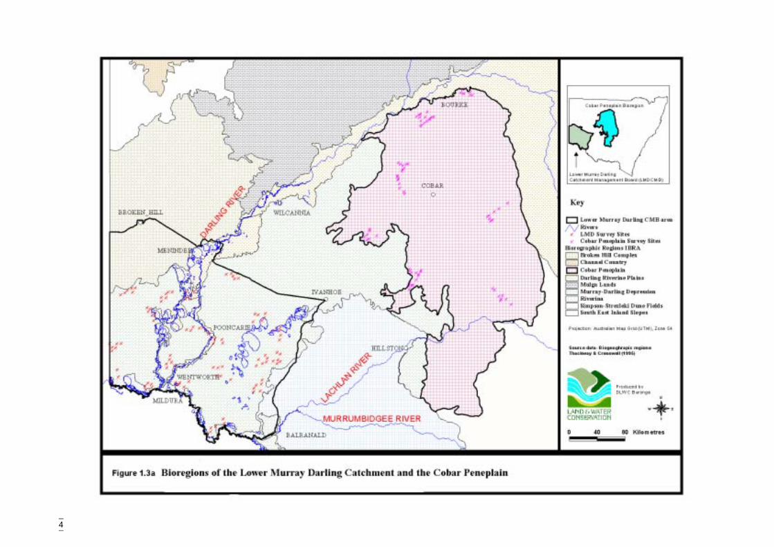
MapsFigure 1.3a Bioregions of the Lower Murray Darling Catchment and the Cobar
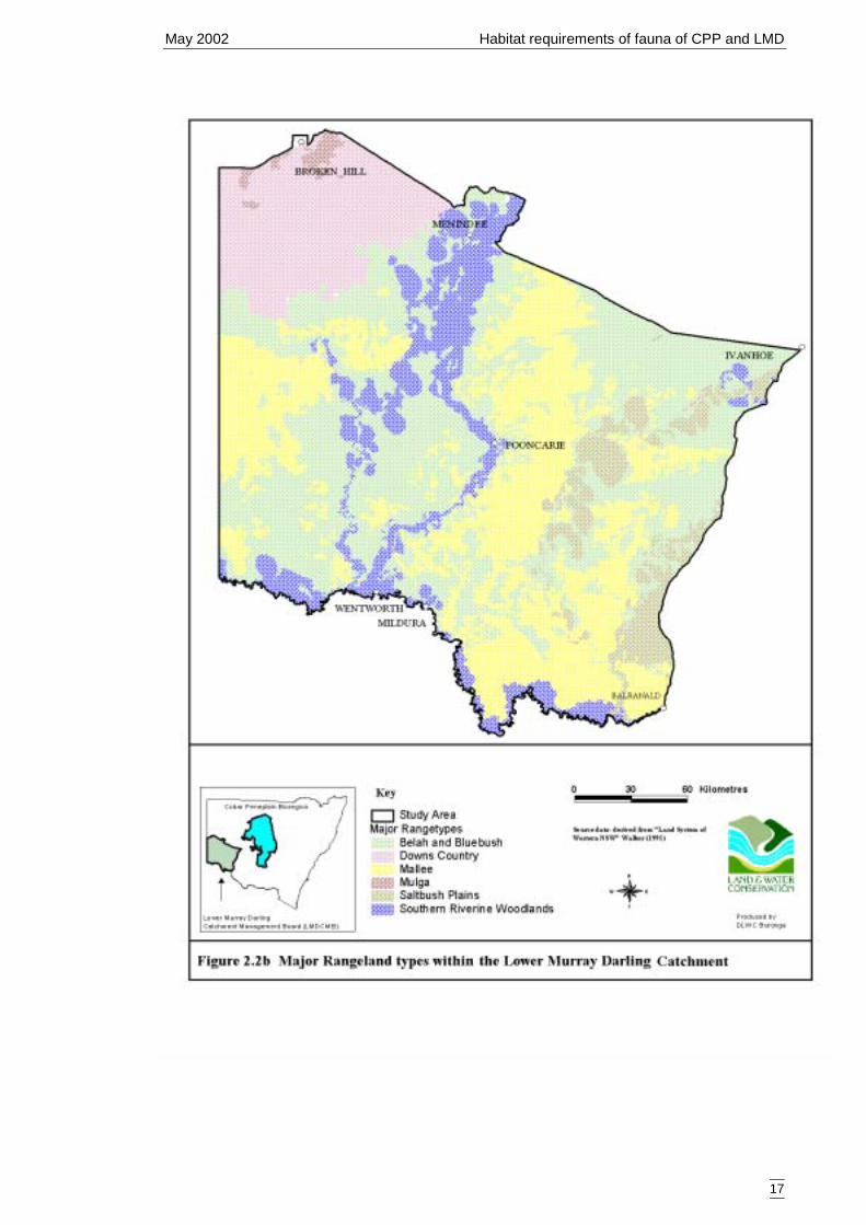
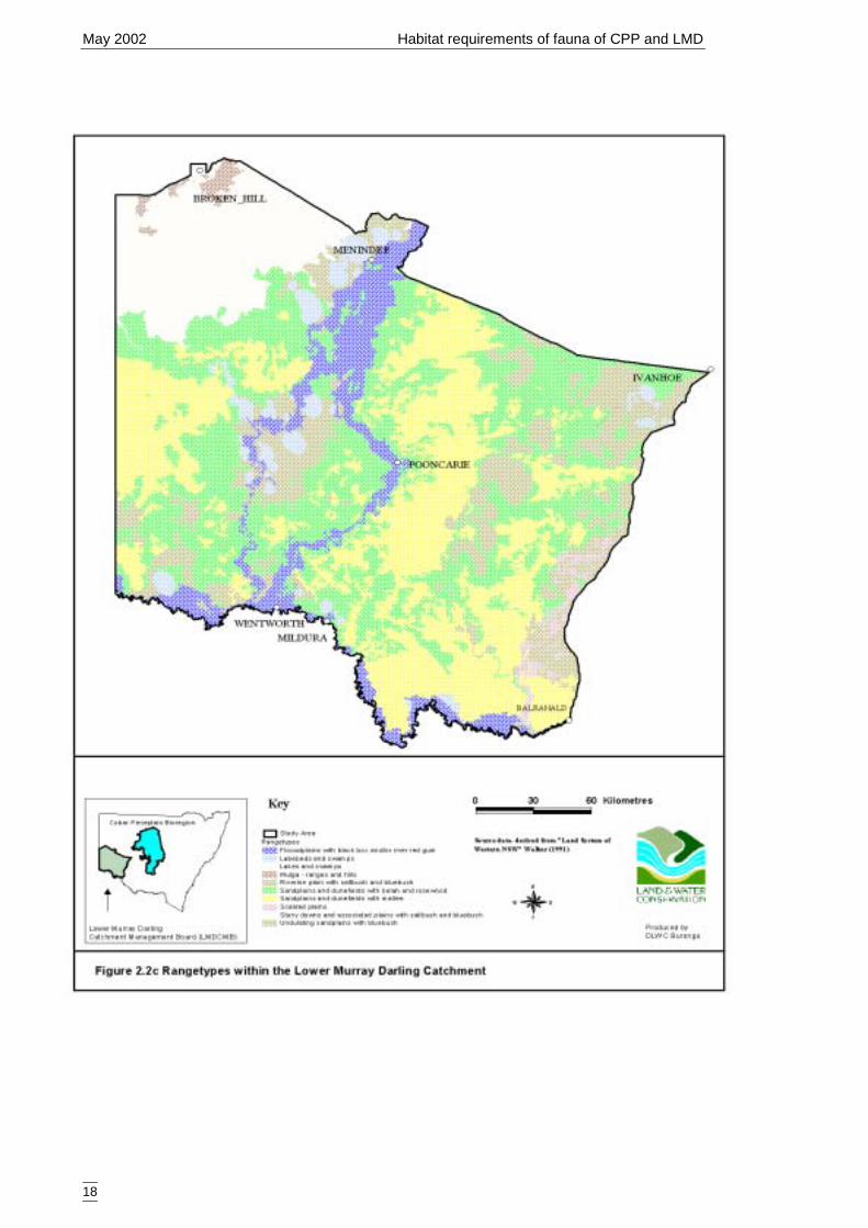
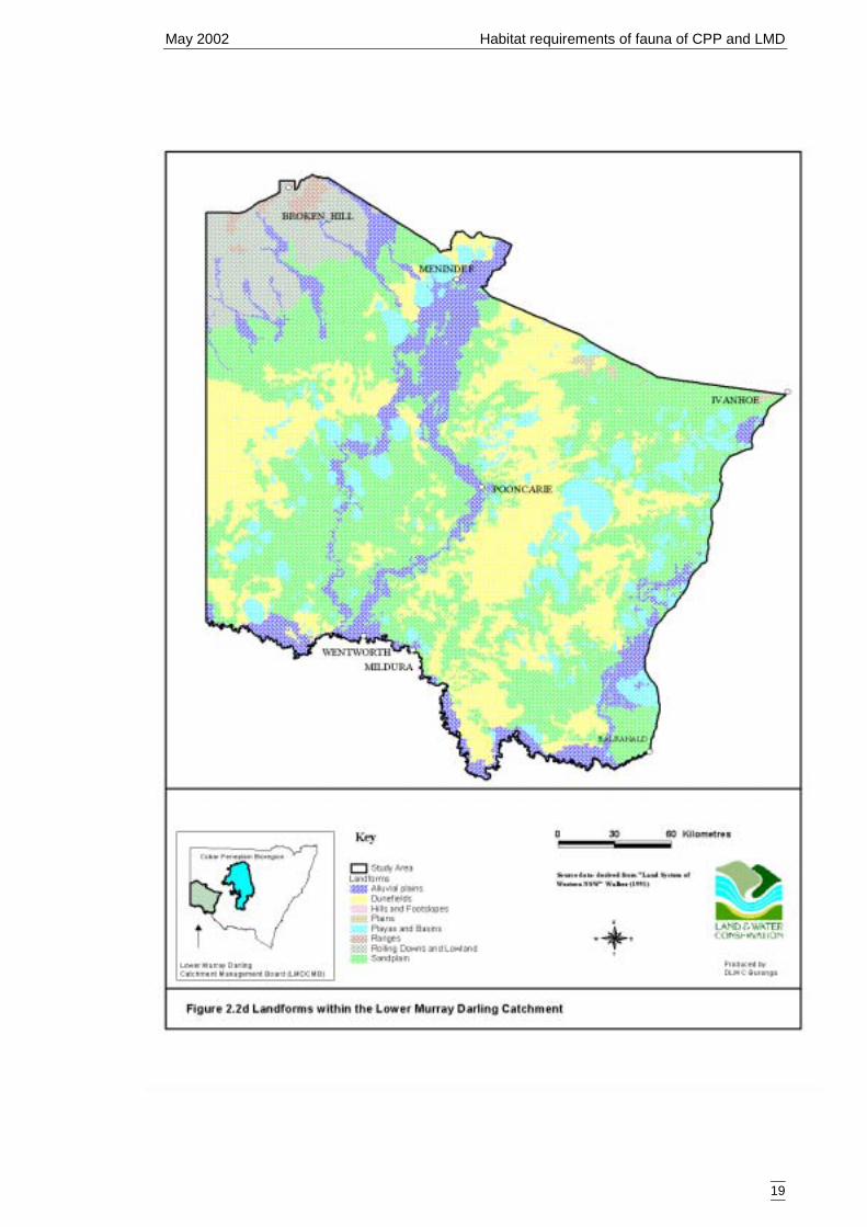
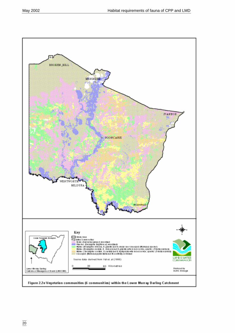
Peneplain ........................................................................................................4Figure 2.2b Major rangeland types within the Lower Murray Darling Catchment.. ......17Figure 2.2c Rangetypes types within the Lower Murray Darling Catchment ...............18Figure 2.2d Landforms within the Lower Murray Darling Catchment ..........................19Figure 2.2e Vegetation communities (6 communities) within the Lower Murray Darling
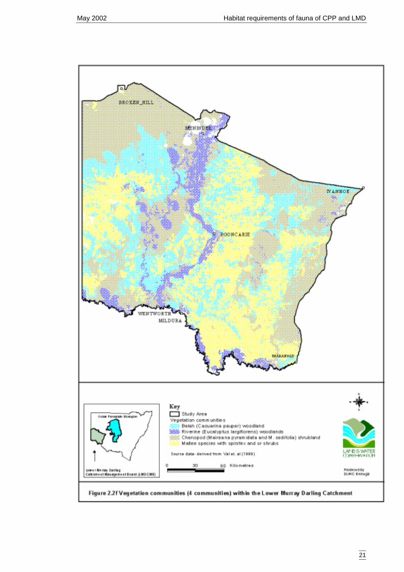
Catchment. ...................................................................................................20Figure 2.2f Vegetation communities (4 communities) within the Lower Murray Darling
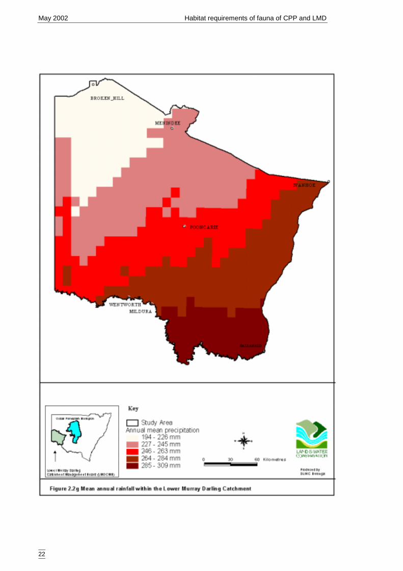
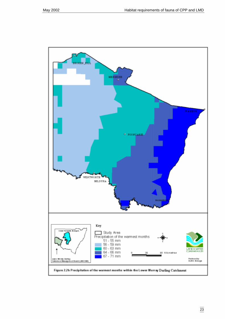
Catchment ....................................................................................................21Figure 2.2g Mean annual rainfall within the Lower Murray Darling Catchment...........22Figure 2.2h Precipitation of the warmest months within the Lower Murray Darling
Catchment ....................................................................................................23
AppendicesAppendix A Vegetation data sheet used in surveys ........................................................86Appendix B Habitat complexity score, based on Catling & Burt (1995). ......................88Appendix C Survey site locations and codes ..................................................................89Appendix D Plant codes referred to in dendrograms and two-way table (listed in
alphabetical order). ....................................................................................92Appendix E Dendogram for sites according to vegetation abundance (beta value = -0.1,
site codes are listed in Appendix C). .........................................................95Appendix F Dendogram for Group II sites according to vegetation abundance (beta
value = -0.2, site codes are listed in Appendix C). ....................................98Appendix G Dendogram for plant species classification (beta value = -0.1, species
codes are listed in Appendix D)...............................................................100Appendix H Dendogram for plant species classification Group 2 (beta value = -0.2,
species codes are listed in Appendix D). .................................................104Appendix I Dendogram for plant species classification Group 2a (beta value = -0.2,
species codes are listed in Appendix D). .................................................107Appendix J Dendogram for plant species classification Group 2b (beta value = -0.2,
species codes are listed in Appendix D). .................................................108Appendix K Two-way table of distribution of perennial plant species (columns indicate
site locations, site codes in Appendix C; rows indicate plant species,species codes in Appendix D)..................................................................109
Appendix L Bird species codes, listed in alphabetic order. ..........................................121Appendix M Dendogram for sites according to bird presence (beta value = -0.1, site
codes are listed in Appendix C). ..............................................................123
Appendix N Dendogram for bird species classification (beta value = -0.1, species codesare listed in Appendix L). ........................................................................126
Appendix O Dendogram for Group 1 bird species classification (beta value = -0.1,species codes are listed in Appendix L)...................................................128
Appendix P Dendogram for Group 1d bird species classification (beta value = -0.1,species codes are listed in Appendix L)...................................................129
Appendix Q Dendogram for Group 3 bird species classification (beta value = -0.1,species codes are listed in Appendix L)...................................................129
Appendix R Two-way table of distribution of bird species (columns indicate sitelocations, site codes in Appendix C; rows indicate bird species, speciescodes in Appendix L). ...........................................................................131
Appendix S Significant terms from primary models, testing on-site habitat variables.137Appendix T Significant terms for secondary models, testing GIS terms. ....................141Appendix U Predicted diversity of bird group 1 (habitat suitability data)....................143Appendix V Predicted diversity of bird group 1 (count data).......................................144Appendix W Predicted diversity of bird group 2 (habitat suitability data)...................145Appendix X Predicted diversity of bird group 2 (count data).......................................146Appendix Y Predicted diversity of bird group 4 (habitat suitability data)....................147Appendix Z Predicted diversity of bird group 4 (count data) .......................................148Appendix AA Predicted diversity of bird group 5 (habitat suitability data using hcs).149Appendix AB Predicted diversity of bird group 5 (habitat suitability data testing hcs
components) ..........................................................................................150Appendix AC Predicted diversity of bird group 5 (count data) ....................................151Appendix AD Predicted diversity of bird group 6 (habitat suitability data).................152Appendix AE Predicted diversity of bird group 6 (count data) ....................................153Appendix AF Summary of effects of habitat variables from primary models on diversity
of bird assemblages. ..............................................................................154Appendix AG Reptile species codes. ............................................................................155Appendix AH Dendogram for sites according to reptile presence (beta value = -0.2, site
codes are listed in Appendix C). ...........................................................156Appendix AI Dendogram for reptile presence classification (beta value = -0.1, species
codes are listed in Appendix AG). ........................................................159Appendix AJ Two-way table of distribution of reptile species (columns indicate site
locations, site codes in Appendix C; rows indicate bird species, speciescodes in Appendix AG). ........................................................................160
Appendix AK Predicted diversity of reptile group 1 (count data) ................................164Appendix AL Predicted diversity of reptile group 3 (habitat suitability data) .............165Appendix AM Predicted diversity of reptile group 3 (count data) ...............................166Appendix AN Predicted diversity of reptile group 5 (habitat suitability data) .............167Appendix AO Predicted diversity of reptile group 5 (count data) ................................168Appendix AP Summary of effects of habitat variables from primary models on diversity
of reptile assemblages. ..........................................................................169Appendix AQ Bat species codes...................................................................................169Appendix AR Dendogram for sites according to bat presence (beta value = -0.1, site
codes are listed in Appendix C). ...........................................................170Appendix AS Dendogram for bat presence classification (beta value = -0.2, species
codes are listed in Appendix AQ). ........................................................172Appendix AT Two-way table of distribution of bat species (columns indicate site
locations, site codes in Appendix C; rows indicate bird species, speciescodes in Appendix AQ). ........................................................................173
Appendix AU Predicted diversity of bat group 1 (count data) .....................................175

Appendix AV Predicted diversity of bat group 2 (habitat suitability data) ..................176Appendix AW Predicted diversity of bat group 2 (count data) ....................................177Appendix AX Summary of effects of habitat variables from primary models on diversity
of bat assemblages. ................................................................................178
References .....................................................................................................................179
Glossary.........................................................................................................................187
PROJECT SUMMARY
i
This report describes a project funded by the NSW Biodiversity Strategy, which was released in1999. As a whole of government document, the Biodiversity Strategy commits all governmentagencies to working cooperatively towards conserving the biodiversity of NSW. The Strategyoutlines a framework for coordinating and integrating government and community efforts toconserve biodiversity across all landscapes.
Project objectivesThe objectives of the project were to:� Determine local scale habitat attributes that describe the preferred habitat of selected faunal
groups of the Cobar Peneplain Bioregion and the Lower Murray Darling Catchment,� Evaluate landscape variables as surrogates for preferred habitat for the same selected faunal
assemblages.� Provide a basis upon which to implement off-reserve conservation measures.� Promote a greater understanding within the community of the region’s biodiversity.� Reduce the cost of resource assessments by providing a regional overview of environmental
values.� Assist in the development and implementation of policies and programmes aimed at
conservation biology in the Lower Murray Darling Catchment.
This technical report is one of two reports specified for the project and specifically addresses thefirst two objectives. The second report will interpret the results of this technical report forpresentation to a wider audience. That document will also develop best management practices thatwill assist in the promotion of a greater understanding of managing the region’s biodiversity.
MethodsFlora and fauna data was collated from the Cobar Peneplain Bioregional Assessment and theLower Murray Darling Environmental Studies. Cluster analysis was used to distinguish floristicand faunal assemblages for birds, bats and reptiles. Faunal assemblages were tested against localor micro-scale habitat variables using generalised linear modelling and predictions of diversity foreach assemblage determined to establish habitat suitability of each site. Habitat suitability wasthen tested against landscape variables for the Lower Murray Darling Catchment, again usinggeneralised linear modelling, to evaluate landscape variables as surrogates. These landscapemodels were spatially interpolated and maps of predicted diversity across the landscape wereproduced. A similar process testing the recorded number of species in each faunal assemblageagainst landscape variables was also conducted.
Key resultsTen faunal assemblages were modelled for which microhabitat predictors of distribution andlandscape surrogates of habitat suitability were successfully identified. Vegetation was the mostfrequently determined local and landscape scale surrogate and proved a good first predictor formany assemblages including generalist bird species, woodland birds, mallee birds, bats and malleereptiles. The response of these and other assemblages to habitat were distinguished further bymicrohabitat variables. For example, log density and vegetation structural attributes separated thedistribution of generalist birds and reptile species. Landscape variables, in particular vegetation,proved to be successful surrogates of habitat suitability but greater explanation of the variation infaunal distribution may be achieved by modelling against the combined microhabitat andlandscape attributes.
Implications for biodiversity conservation managementVegetation was determined as the best first predictor of faunal distribution and habitat suitabilityand is a good first consideration for reserve selection. However, a comprehensive range of taxawill not be conserved using this single attribute. The complex relationship between speciesdistribution and finer-scale attributes creates habitat specialists whose requirements may not bemet within large reserves selected without consideration of microhabitat conditions. Distributionmaps of preferred habitat can be used as a tool against the threat of clearing but need to be verifiedbefore use in conservation plans. Best management practices designed to maintain habitat qualityoutside existing reserves need to be developed.
June 2002 Habitat requirements of fauna of CPP and LMD
1
1 INTRODUCTION
1.1 BACKGROUND
The NSW Biodiversity Strategy was implemented to address the loss of biodiversityacross NSW and this current project was designed to meet one of the priority actions ofthe Strategy. This action requires the acceleration of the outcomes of the CobarPeneplain Bioregional Assessment and is listed under Section 2: Conservation andprotection of biodiversity, Objective 2.1: Implement bioregional assessment andplanning throughout NSW and Priority Action 13: Bioregional planning.
This project extends work initiated by the Cobar Peneplain Bioregional Assessment,particularly the work investigating fauna distribution. The outcomes of the faunainvestigation included a recommendation for incorporating additional data from othersurveys into the Cobar Peneplain database (Masters & Foster 2000). The need for awider geographical spread of sites was stressed to obtain significant predictions for thedistribution and habitat requirements of fauna species.
A proposal for this project was put forward by the Department of Land and WaterConservation for a project to be jointly funded by the NSW Biodiversity Strategy, NSWNational Parks and Wildlife Service and the Department of Land and WaterConservation. This project would utilise fauna and habitat records from the CobarPeneplain Bioregion and the Lower Murray Darling Catchment to further investigatefauna habitat requirements. The bioregions of the catchment are contiguous with theCobar Peneplain Bioregion and many flora and fauna species are found across bothregions, justifying the use of both data sets.
1.2 OBJECTIVES
The objectives of the project were to:
� Determine local scale habitat attributes that describe the preferred habitat of selectedfaunal groups of the Cobar Peneplain Bioregion and the Lower Murray DarlingCatchment,
� Evaluate landscape variables as surrogates for preferred habitat for the sameselected faunal assemblages.
� Provide a basis upon which to implement off-reserve conservation measures.� Promote a greater understanding within the community of the region’s biodiversity.� Reduce the cost of resource assessments by providing a regional overview of
environmental values.� Assist in the development and implementation of policies and programmes aimed at
conservation biology in the Lower Murray Darling Catchment.
June 2002 Habitat requirements of fauna of CPP and LMD
2
This technical report is one of two reports specified for the project and specificallyaddresses the first three objectives. The second report will interpret the results ofthis technical report for presentation to a wider audience. That document will alsodevelop best management practices that will assist in the promotion of a greaterunderstanding of managing the region’s biodiversity.
1.3 STUDY AREA
The information below is taken from Masters & Foster (2000) and Val et al. (2001).
1.3.1 Location and areaThe Cobar Peneplain covers approximately 73 500 square kilometres (Figure 1.3a). Itspans central and far-western NSW and extends from Bourke in the north to Griffith inthe south. It is bounded by the Darling and Bogan Rivers in the north-west and north-east respectively. The townships of Cobar, Canbelego, Nymagee, Mt Hope, EubalongWest, Lake Cargelligo and Rankin Springs are located within its boundaries whilstLouth, Nyngan, Tottenham, Tullamore, Condobolin and Griffith lie along itsboundaries.
The Lower Murray Darling Catchment is approximately 60 100 square kilometres(Figure 1.3a). The catchment is bounded by the Murray River in the south and extendsnorthwards to Broken Hill and Ivanhoe and from the South Australian border east toBalranald. Leasehold land is the major land tenure, covering more than 90% of thecatchment (DLWC GIS).
About 60% of the Cobar Peneplain and the entirety of the Lower Murray DarlingCatchment lie within the Western Division administrative area of NSW. The remaining40% of the Cobar Peneplain lie in the Central Division. Lands in the Western Divisionare predominantly leasehold tenure and those of the Central Division are predominantlyfreehold. This difference in tenure between west and east has resulted in differingmanagement practices across this divide. For example, the Central Division is moreintensively cultivated and more extensively cleared of native vegetation when comparedto the Western Division, where the predominant land use is pastoralism, with extensiveclearing having been restricted by the lease conditions.
Eight local government areas lie wholly or partly within the Cobar Peneplain Bioregion.These are Bourke, Bogan, Brewarrina, Bland, Carrathool, Lachlan, Cobar andNarrandera. The Lower Murray Darling Catchment encompasses the entire LocalGovernment areas of Wentworth and Broken Hill City, most of the Shire of Balranaldand parts of the Central Darling Shire and the unincorporated area of NSW.
1.3.2 BioregionsAustralia is divided into bioregions that represent interacting ecosystems classified bydominant landscape features such as geology, landform, climate and vegetation(Thackway & Cresswell 1995).
The Cobar Peneplain is characterised by landforms of rolling downs and plainsdominated by woodlands of bimble box, white cypress pine, mulga, red box, belah andmallee. It is a semi-arid area with rainfall ranging from 360mm in the north-west toabout 500mm in the south-east. Rainfall is highly variable over the whole region and
June 2002 Habitat requirements of fauna of CPP and LMD
3
prolonged periods of low rainfall with intermittent floods are characteristic (Pickard &Norris 1994). Rainfall is summer-dominant in the north of the region and winter-dominant in the south. From November to March is the hottest period, with frequentmaximum daily temperatures in excess of 38oC. The coldest month is July and frequentfrosts occur between June and August.
Four bioregions occur in the Lower Murray Darling Catchment (Thackway & Cresswell1995) (Figure 1.3a). These are:
� The Murray Darling Depression Bioregion (72%, 4 305 128 hectares) constitutesthe majority of the catchment. It lies on either side of the Darling River and is thebioregion most extensively used for dryland cropping and grazing. It ischaracterised as an undulating sand and clay plain with wind-blown dunes and isgeologically young; most features date to the Tertiary or Quaternary age.
� The Darling Riverine Plains Bioregion (8%, 495 330 hectares) follows theDarling River Corridor from the north of the study area and is predominantlyalluvial fans and plains of grey clay soils covered by Eucalyptus dominatedwoodlands.
� The Riverina Bioregion (6%, 373 262 hectares) is an ancient riverine plain withalluvial fans extending along the Murray River. Sediments are unconsolidatedand vegetation is varied, however red gum, black box, swamps and saltbushshrublands are characteristic in the NSW Lower Murray Darling area.
� The Broken Hill Complex (14%, 838 413 hectares) consists of rocky hills andcolluvial fans, with desert loams (sometimes calcareous), clays and lithosols inlower areas. Shrublands and mulga dominate the vegetation.
The Lower Murray Darling Catchment is in the semi-arid region of NSW and has awinter dominant rainfall. Average rainfall ranges from 355mm in the east to 200mm inthe west. During summer rainfall is low throughout the area. Low summer rainfall isalso accompanied by high evaporation rates. Temperature varies little across the studyarea. Temperature ranges from average overnight lows of 3°C to average daytimemaximums of 34°C. Recordings of below 0°C in winter and above 40°C in summer canoccur.
Five broad vegetation types occur within the Lower Murray Darling Catchment,determined largely by edaphic and climatic factors (Cunningham et al. 1992). Theseinclude belah woodlands on red earths, dense mallee communities on sandplains anddunefields, bluebush shrublands on brown or grey clays, riverine communities of blackbox and/or red gum and a small area of mulga shrublands on sandplains and ranges inthe north-west of the catchment.
4
June 2002 Habitat requirements of fauna of CPP and LMD
5
2 METHODS
2.1 DATA COLLECTION
Fauna and flora data were obtained from existing sources. Data from the CobarPeneplain Bioregional Assessment (Masters & Foster 2000) and the Lower MurrayDarling Environmental Studies (Val et al. 2001) were incorporated into a singledatabase.
A requirement for combining data from different surveys is compatibility of surveymethodology. Both the Cobar Peneplain Bioregional Assessment and the Lower MurrayDarling Environmental Studies employed similar survey techniques. Methods for faunacollection and vegetation surveys are taken from Masters & Foster (2000) and Val et al.(2001) and a brief description of the methods used in these studies follows below.
Birds, bats and reptiles were the primary fauna targeted and to maximise the probabilityof detection the surveys were conducted during the warmer months of the year.Terrestrial mammals were also surveyed but captured rates were too low for furtheranalysis. Surveying for the Lower Murray Darling Environmental Studies took placefrom September 1998 - April 1999 and October 1999 - March 2000 and totalled 114sites. The Cobar Peneplain Bioregional Assessment surveys took place from November1997 - late April 1998, covering 80 sites.
2.1.1 Site selection and samplingThe survey sites were selected using a stratified survey design based on vegetation (tosample as diverse a range of vegetation types as possible), geographical spread anddistance from water. More detail on site selection can be obtained from the relevantreports (Masters & Foster 2000, Val et al. 2001). Table 2.1
Bird and reptile surveys were conducted within a 3 hectare site. A 100 metre x 100metre vegetation and habitat sub-site was located within the 3 hectare site.
2.1.2 Vegetation and habitatVegetation data included structural details (after Specht 1970) and cover/abundanceestimates of dominant species as determined by a modified Braun-Blanquet method(Appendix A).
Structural information included the height of each vegetation layer and the projectivefoliage cover (measured as the percent shadow cast when the sun is overhead) of thedominant species within each layer. Each structural layer of herb, grass, shrub <0.25metre, shrub 0.25 - 2 metre, shrub >2 metre, tree < 10 metre, tree 10 - 30 metre and tree>30 metre was assigned to one of the cover categories 0%, <10%, 10 - 30% and 30 -50%. Some categories were combined if the frequencies were considered too low for
June 2002 Habitat requirements of fauna of CPP and LMD
6
analysis (see Results section). The dominant species from each structural layer weregiven a Braun-Blanquet cover/abundance estimate. All other species detected at a sub-site were recorded as present.
The microhabitat attributes collected from each 1 hectare sub-site were the presence orabsence of disturbance, the type of disturbance, type of herbivore, evidence of past fireand surface soil texture, soil depth and indication of moisture level. Within a 20 x 20metre sub-site of the 1 hectare site, the number of logs greater than 5 centimetresdiameter, number of hollow logs, the presence of tree hollows and the cover and type ofsurface strew were also noted. The percent litter and cryptogam (lichen, moss andcyanobacteria) cover were averaged from ten 1 m2 plots, each plot 1 metre apart.
2.1.3 BirdsMultiple bird censuses were conducted at each site, each of 30 minutes duration andundertaken on different days and at different times of the morning to maximise birddetection. Sampling took place from sunrise for approximately 3 hours. Counts weremade of birds within the 3 hectare site or flying over the site and were identified fromtheir calls and by observation. The Lower Murray Darling Environmental Studiessurvey conducted two morning censuses per site while the Cobar Peneplain BioregionalAssessment conducted three morning and one late afternoon census. Preliminaryanalysis showed that the additional afternoon and morning census did not contributesubstantially to the species diversity of a site and therefore bias would be minimal.
2.1.4 BatsInsectivorous microchiropteran bats were surveyed with harp traps and an ultrasonicAnabat TM ‘bat-detector’ recorder. Harp traps intercept and trap bats in flight while theAnabat TM records ultrasonic calls that can be used to identify species. Species that flyabove and below the canopy can be detected in this way.
All sites were sampled, using with the Anabat TM ’bat detector’, except in wet or windyweather, for a period of 30 minutes. Recording commenced between dusk and threehours after dusk. One harp trap per site was set to intercept below canopy species andwas opened for three (Cobar Peneplain Bioregional Assessment) or four (Lower MurrayDarling Environmental Studies) nights. Bats were identified, marked with a liquidmarker and held in a cool place until their release at point of capture in the evening.
2.1.5 ReptilesDiurnal searchesEach site was sampled for one person-hour. Sampling was conducted in the earlymorning hours before temperatures became too warm. Extremely hot parts of the daywere avoided as reptile activity is low and those species that are active are quickmoving and difficult to correctly identify. Potential habitats such as logs, leaf litter,burrows, shrubs and spinifex were examined and the number of each species wasrecorded.
Nocturnal searchesEach site was sampled for a period of one person-hour after sunset and beforetemperatures became too cool, with the number of each species being recorded.Sampling on cold, windy or rainy nights was avoided. The Lower Murray DarlingEnvironmental Studies conducted nocturnal surveys once each site and the CobarPeneplain Bioregional Assessment surveyed each site twice.
June 2002 Habitat requirements of fauna of CPP and LMD
7
2.1.6 NomenclatureVertebrate nomenclature followed the CSIRO list of Stanger et al. (1998). Reptileidentification followed Cogger (1992) and Swan (1990), amphibian identificationfollowed Cogger (1992) and Robinson (1993), bat identification followed Parnaby(1992) and Churchill (1998), rodent identification followed Dickman (1993) anddasyurid identification followed Dickman and Read (1992). Strahan (1983) and Triggs(1996) were also used for mammal identification. Bird identification followed Simpsonet al. (1999).
Plant nomenclature and identification followed Harden (1990, 1991, 1992, 1993) andcommon names were taken from Cunningham et al. (1992) and Hart (1995).
2.2 DATA ANALYSIS
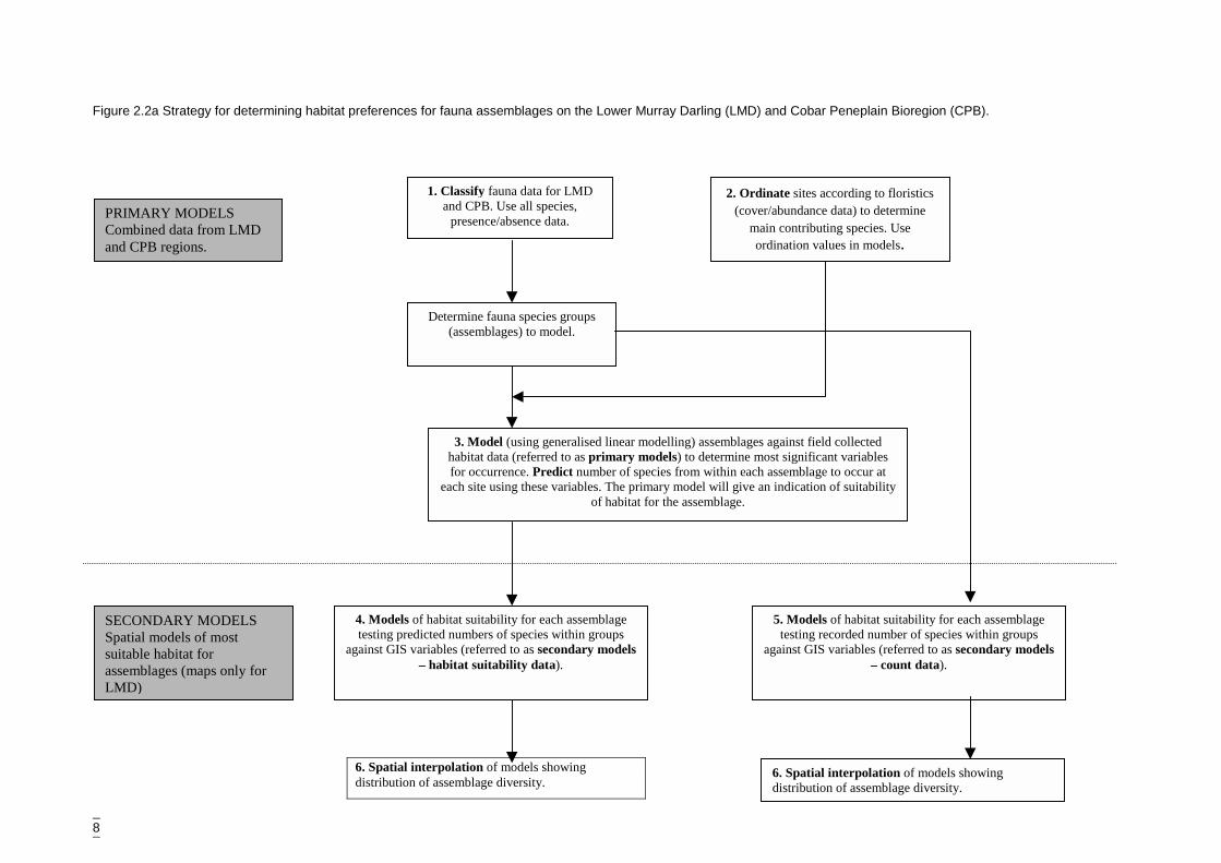
The analysis of the vegetation and fauna data involved six steps:1. Classification of sites according to both floristic cover/abundance and fauna
presence and classification of species associations.2. Ordination of sites according to floristic cover/abundance.3. Generalised linear modelling of the number of species from each fauna species
classification group against field-collected habitat data (the primary model). Predictnumber of species expected to occur at sites within the Lower Murray DarlingCatchment. Predicted number of species used as a measure of habitat suitability ofeach site,
4. Generalised linear modelling of habitat suitability of each site against remotelymapped GIS variables (a secondary model),
5. Generalised linear modelling of the number of species from each fauna speciesclassification group against remotely mapped GIS variables (a secondary model) forthe Lower Murray Darling Catchment, and
6. Spatial interpolation of the secondary models for the Lower Murray DarlingCatchment.
This analysis pathway is summarised in Figure 2.2a.
It was felt that the aim of regional conservation assessment could be better met bystudying species groups as opposed to individual species. Specific habitat informationfor single species would not be available but habitat requirements for assemblageswould provide a more robust basis for predicted abundance distributions across theregion. The problem of relatively small numbers of data points for single species,particularly threatened species, would be overcome by analysing (modelling)assemblages. It is therefore assumed that conserving for the assemblage will includeconserving for any species within the assemblage.
8
Figure 2.2a Stra
PRIMARY MCombined datand CPB regi
SECONDARSpatial modelsuitable habitaassemblages (LMD)
tegy for determining habitat preferences for fauna assemblages on the Lower Murray Darling (LMD) and Cobar Peneplain Bioregion (CPB).
1. Classify fauna data for LMDand CPB. Use all species,
presence/absence data.
Determine fauna species groups(assemblages) to model.
2. Ordinate sites according to floristics(cover/abundance data) to determine
main contributing species. Useordination values in models.
3. Model (using generalised linear modelling) assemblages against field collectedhabitat data (referred to as primary models) to determine most significant variablesfor occurrence. Predict number of species from within each assemblage to occur at
each site using these variables. The primary model will give an indication of suitabilityof habitat for the assemblage.
4. Models of habitat suitability for each assemblagetesting predicted numbers of species within groups
against GIS variables (referred to as secondary models– habitat suitability data).
ODELSa from LMD
ons.
Y MODELSs of mostt formaps only for
5. Models of habitat suitability for each assemblagetesting recorded number of species within groups
against GIS variables (referred to as secondary models– count data).
6. Spatial interpolation of models showingdistribution of assemblage diversity.
6. Spatial interpolation of models showingdistribution of assemblage diversity.
June 2002 Habitat requirements of fauna of CPP and LMD
9
2.2.1 ClassificationSites were classified using the computer software programme PATN (Belbin 1995) toidentify patterns in species (plant and animal) distribution. Species classification wasalso conducted to identify species associations. The vegetation data was ordinated toidentify specific gradients across the sites. The faunal species classification groups werethen examined for relationships with the vegetation gradients.
The vegetation and faunal data were classified using the general pathways describedbelow, following strategies used in similar studies (e.g. Forward & Robinson 1996,McKenzie et al. 1991, Masters & Foster 2000). Site classification produces groups ofsites with similar species composition while species classification generates groups ofspecies with similar distributions. The construction of a two-way table was used toillustrate fauna occurrence across sites.
Single occurrences of plant species were excluded from the analysis and thecover/abundance ratings were ranked. Single occurrences of bird and reptile specieswere excluded from consideration and the abundance data converted topresence/absence.
Site classificationSites were classified separately for flora, birds, reptiles and bats. An association matrixwas created using the Bray-Curtis coefficient of dissimilarity (ASO module) todetermine the level of association between sites. An agglomerative hierarchicalclustering algorithm, flexible UPGMA (Unweighted Pair Group arithMetic Averaging)was employed (FUSE module) to create the groups. The beta value was set at � = -0.1unless otherwise stated. The variation in the beta value allows for space dilation (orcontraction) and is better for extracting ‘true’ groups from ecological data (Belbin1995).
A dendogram (DEND module) was used to display the results of the clustering andillustrate the relationships between the sites. The determination of the number of groupsis largely subjective, ensuring that ecologically meaningful groups can be created, basedon the author’s knowledge of semi-arid flora and vertebrate fauna. Groups were definedusing the group definition module (GDEF). The significance level (given as a pseudo F-ratio) of the groups is determined using a between-group mean dissimilarity comparedto a within-group mean dissimilarity via an ANOSIM randomisation (ASIM).
The site groups were explored for 'principal' species using the group statistics (GSTA)module. The GSTA module presents a Kruskal-Wallis value for each species as anindicator of the level of association. Species with values larger than 7 and p < 0.05 wereassigned to a group. 'Principal' species were defined either as species that achieved ahigh Kruskal-Wallis value or were considered to be important to the group basedknowledge of the survey region.
Species classificationSpecies (flora and fauna) analysis was conducted by transposing the data (DATN) toproduce a matrix of species by sites. The species were then range standardised. TheASO-FUSE-DEND-GDEF analysis steps outlined above were followed, however the Bray-Curtis measure of association was replaced with the two-step measure of association, asit is more suited for species classification. The two-step measure is a modification of the

June 2002 Habitat requirements of fauna of CPP and LMD
10
Bray-Curtis measure to account for asymmetric associations between species (Belbin1995).
Evaluation of classificationThe final step in the classification process was the construction of a two-way table usingthe TWAY module to evaluate the site and species classifications and to further assistwith identifying the best site groupings.
2.2.2 OrdinationOrdination is the arrangement of sites along gradients on the basis of speciescomposition and allows for the representation of sites in space showing the relationshipbetween sites. Sites close together are similar in species composition. The ordinationvalues determined from the floristics data were used as variables in the primary modelsand were chosen to reduce the complexity inherent is testing individual plant species.
The sites were ordinated using non-metric semi-strong hybrid multidimensional scaling(SSH) and the axes rotated (PCR) (Belbin 1995). The choice of the number ofdimensions or axes used to describe the data is subjective and is a compromise betweentoo few and too many. Too few dimensions and there will be too many constraints foreffective placement of sites, too many and the sites are unconstrained, creating noise(Belbin 1995). The number can be determined by calculating the stress level (badness offit) produced from 10 random starts for 1 – 5 dimensions and producing a scree plotversus the number of dimensions. The optimum number of dimensions is achievedwhen the decrease in the stress is no longer large for an increase in dimensionality(Faith & Norris 1989). Four dimensions were determined as optimal for the vegetationdata.
The species correlations to the ordination axes were examined by use of a multiple-linear regression programme, Principal Axis Correlation (PCC). The resultantcorrelation coefficients were tested for significance using a Monte-Carlo test with 100randomisation (MCAO). Significant (p < 0.05) species with r values greater than 0.6were selected as best describing the gradients along each axis.
2.2.3 ModellingGeneralised linear modelling (GLM) is a form of multiple regression that accommodatesa wide range of error and link functions and has been applied extensively to themodelling of species distributions (Bos et al. 2002, Catling et al. 1998, 2000, Claridge& Barry 2000, Claridge et al. 2000, Read et al. 2000). It is an extension of linearregression modelling that allows the specification of error structures in addition to thenormal distribution. The assumption is that the response variable is linearly related to aset of measured explanatory variables or predictors. The linear model can be written as
yi = a + � bjxij + ei
where yi is the observed response for sample i, x ij are the j predictor variables, a and bjare parameters to be estimated from the data, and ei is a random error component withmean and variance from the exponential family of distributions (McCullagh & Nelder1989).
Three components must be defined for a GLM: an error function, a linear predictor, anda link function:
June 2002 Habitat requirements of fauna of CPP and LMD
11
� The Poisson error family was used for the count data. The response variableswere the number of species within a group at a site. These are count data and arebest described by the Poisson probability distribution.� The linear predictor (LP) is defined as the sum of the effects of the predictor
variables:
LPi=a + bxi1 + cxi2 +…….
where a, b, c are parameters to be estimated from the observed data. Theseparameters define the effect of the variables on the linear predictor and henceon the estimated probability of recording the species. The xi1, xi2 are thepredictor variables, for example continuous variables such as annual rainfall, orfactor data such as vegetation type, where different classes are recognised.
� A log link function was used to fit the count data. The link function relates themean value of y to its linear predictor. In the case of count data the log linkensures that negative fitted values are not calculated. The predicted valued of yis obtained by applying the inverse of the link function to the linear predictor:
Predicted response=explinear predictor
Generalised linear models were fitted using the Splus6 (Insightful 2001) statisticalsoftware package. Models were constructed using a forward stepwise procedure forselecting environmental predictors (ie. environmental variables) for groups of species.
The terms of the model were estimated using a forward stepwise procedure as describedby Nicholls (1991). This process starts with each variable being fitted as a series ofnested models and noting the reduction in residual deviance for each successive modelfit. The significance of each change in deviance is examined by a Chi-square test (at thep < 0.05 significance). Deviance is a measure of the closeness of fit of a model to theobserved data from which it was derived. The smaller the deviance the better the model(i.e. the stronger the environmental relationship). The variable that was most significantwith the greatest reduction in residual deviance was added to the model. This processwas repeated using all the remaining variables. The model fitting process was repeateduntil the addition of additional variables no longer resulted in a significant reduction inthe model deviance. Quadratic terms were also tested to determine the significance ofany non-linear relationships within the model.
The random error component of the model is often more variable than expected for aPoisson distribution and is not uncommon for fauna counts. This is known asoverdispersion and indicates a clustered distribution of the data (Read et al. 2000). Ifafter the initial fit overdispersion was evident, either a negative binomial or quasi familywas nominated on subsequent passes. However, many of the secondary modelsinvolving predicted values as the response (see below) were underdispersed indicating amore uniform than random distribution but were not treated differently on subsequentpasses.
Once the most significant terms were identified, interactions between the terms weretested. A model containing an interactive term was chosen only if the residual deviancewas smaller than the previous model. Once all terms were identified, the model wassimplified by investigating which terms could be deleted from the model. Terms were
June 2002 Habitat requirements of fauna of CPP and LMD
12
retained only if their removal caused a significant increase in deviance. Finally, non-significant (t value < 1.5) levels of factor variables were merged.
Primary modelsThe prime purpose of the primary models was to provide a set of attributes that wouldenable the assessment of independent sites for their suitability for a particular faunalassemblage. The primary model presents the local-scale habitat or microhabitatconditions that best fit the response i.e. the field variables that best fit each speciesgroup. These field variables therefore describe each species group’s preferredmicrohabitat. The predicted number of species expected to occur within a subset of thedata, namely the Lower Murray Darling Catchment sites, was then calculated for eachspecies group. The predicted number of species from the assemblage can be considereda measure of the habitat suitability of the site - a higher number of species indicates ahigher preference for the site. These values were used in a second round of modelling(secondary models) designed to test the microhabitat suitability of sites against remotelymapped variables within the Lower Murray Darling Catchment.
Field-based variables used for primary modelsThe variables used in the primary models are listed in Table 2.2a. These variables wererecorded on-site, determined from the ordination or derived from site information (e.g.habitat complexity score). Some vegetation structural levels were infrequently recordedand were amalgamated into the most similar category. These amalgamated attributes aresummarised in Table 2.2b.
The habitat complexity score is a modified version of one devised by Catling & Burt(1995) and is an amalgamation of several structural features. These are outlined inAppendix B. A high score (greater than 10) indicates a structurally complex site withwoodland cover, high litter cover, log density and tree hollows. A low score indicates arelatively less complex site.
Secondary modelsThese models were developed only for the Lower Murray Darling Catchment and weredesigned to predict distribution across a region using remotely mapped variables. Theaims of the secondary models were to:� identify the remotely mapped GIS surrogates that were significant for each species
group,� predict the diversity of each species group according to the landscape variables and,� spatially interpolate the model to derive the distribution of faunal assemblage
diversity.
The secondary models tested two different responses against GIS variables:� the predicted number of species from each group (determined from the primary
models) which are referred to as habitat suitability models, and� the recorded number or count of species within each species group, referred to as
count models.A Poisson distribution and a log-link function were specified for both sets of models.
The GIS coverages that were tested were landsystems, vegetation communities(determined from previous analysis of vegetation for the Lower Murray DarlingCatchment (Val et al. 2001)) and rainfall.
Land systems can be defined as ‘an area or group of areas throughout which there is arecurring pattern of topography, soil and vegetation’ (Christian 1958). The total number
June 2002 Habitat requirements of fauna of CPP and LMD
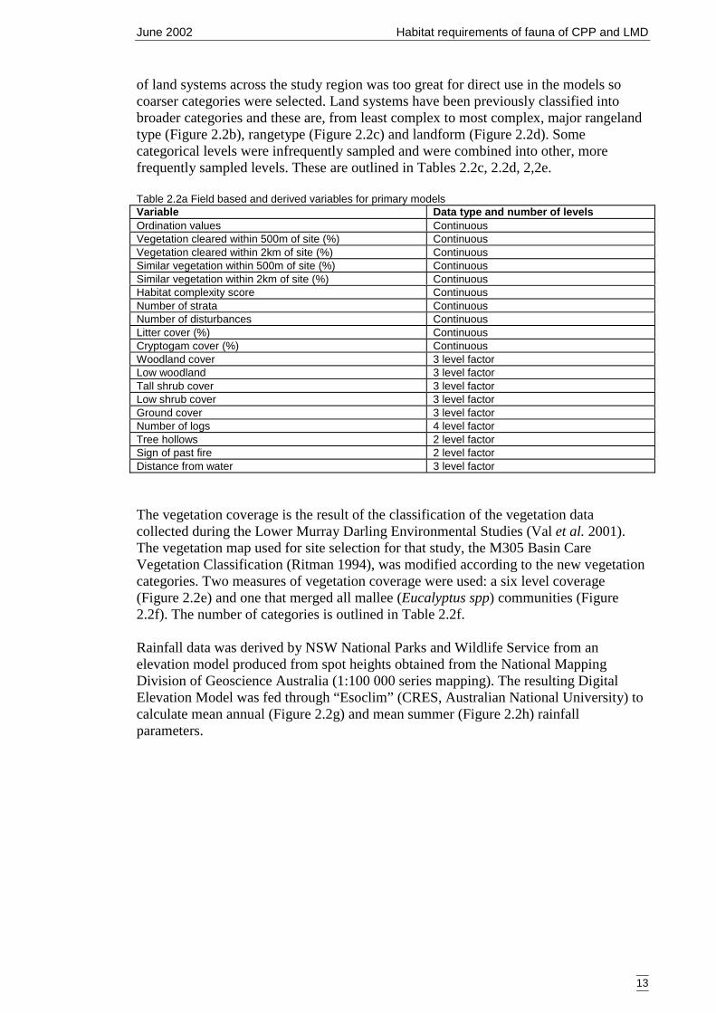
13
of land systems across the study region was too great for direct use in the models socoarser categories were selected. Land systems have been previously classified intobroader categories and these are, from least complex to most complex, major rangelandtype (Figure 2.2b), rangetype (Figure 2.2c) and landform (Figure 2.2d). Somecategorical levels were infrequently sampled and were combined into other, morefrequently sampled levels. These are outlined in Tables 2.2c, 2.2d, 2,2e.
Table 2.2a Field based and derived variables for primary modelsVariable Data type and number of levelsOrdination values ContinuousVegetation cleared within 500m of site (%) ContinuousVegetation cleared within 2km of site (%) ContinuousSimilar vegetation within 500m of site (%) ContinuousSimilar vegetation within 2km of site (%) ContinuousHabitat complexity score ContinuousNumber of strata ContinuousNumber of disturbances ContinuousLitter cover (%) ContinuousCryptogam cover (%) ContinuousWoodland cover 3 level factorLow woodland 3 level factorTall shrub cover 3 level factorLow shrub cover 3 level factorGround cover 3 level factorNumber of logs 4 level factorTree hollows 2 level factorSign of past fire 2 level factorDistance from water 3 level factor
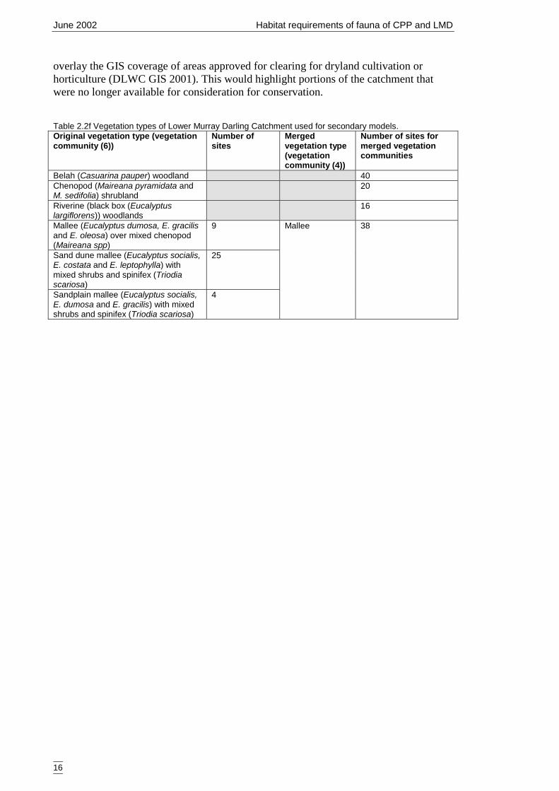
The vegetation coverage is the result of the classification of the vegetation datacollected during the Lower Murray Darling Environmental Studies (Val et al. 2001).The vegetation map used for site selection for that study, the M305 Basin CareVegetation Classification (Ritman 1994), was modified according to the new vegetationcategories. Two measures of vegetation coverage were used: a six level coverage(Figure 2.2e) and one that merged all mallee (Eucalyptus spp) communities (Figure2.2f). The number of categories is outlined in Table 2.2f.
Rainfall data was derived by NSW National Parks and Wildlife Service from anelevation model produced from spot heights obtained from the National MappingDivision of Geoscience Australia (1:100 000 series mapping). The resulting DigitalElevation Model was fed through “Esoclim” (CRES, Australian National University) tocalculate mean annual (Figure 2.2g) and mean summer (Figure 2.2h) rainfallparameters.
June 2002 Habitat requirements of fauna of CPP and LMD
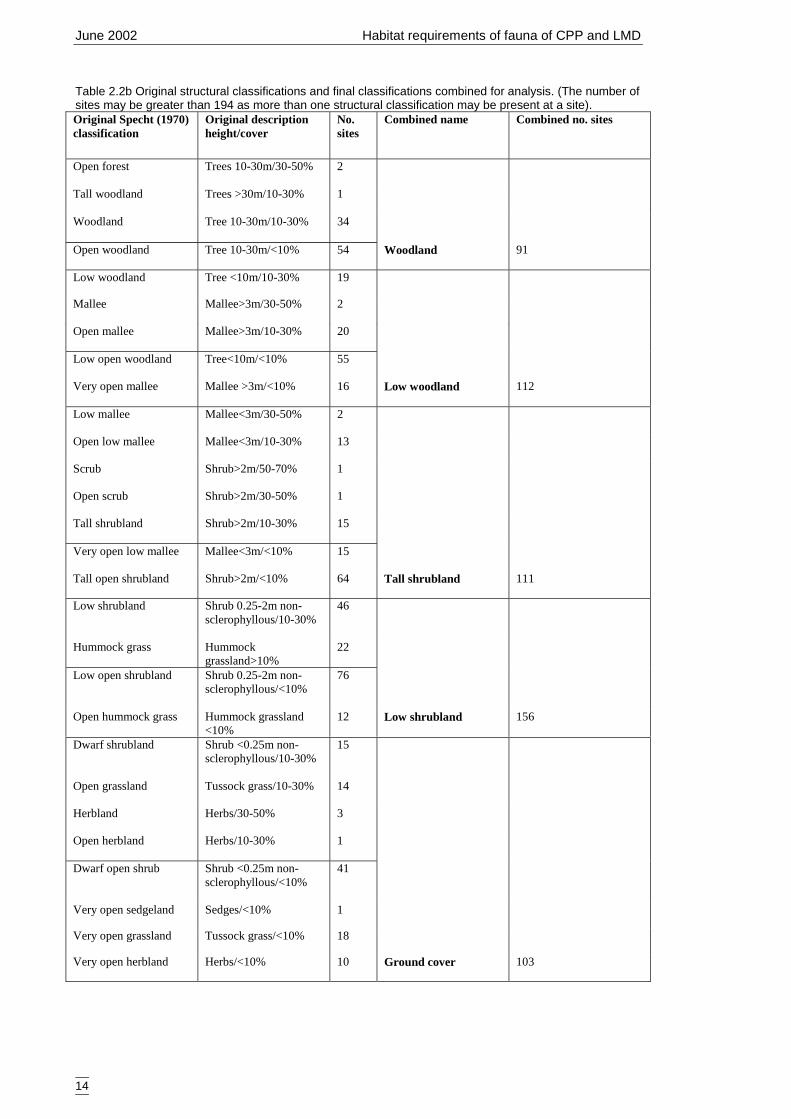
14
Table 2.2b Original structural classifications and final classifications combined for analysis. (The number ofsites may be greater than 194 as more than one structural classification may be present at a site).Original Specht (1970)classification
Original descriptionheight/cover
No.sites
Combined name Combined no. sites
Open forest Trees 10-30m/30-50% 2
Tall woodland Trees >30m/10-30% 1
Woodland Tree 10-30m/10-30% 34
Open woodland Tree 10-30m/<10% 54 Woodland 91
Low woodland Tree <10m/10-30% 19
Mallee Mallee>3m/30-50% 2
Open mallee Mallee>3m/10-30% 20
Low open woodland Tree<10m/<10% 55
Very open mallee Mallee >3m/<10% 16 Low woodland 112
Low mallee Mallee<3m/30-50% 2
Open low mallee Mallee<3m/10-30% 13
Scrub Shrub>2m/50-70% 1
Open scrub Shrub>2m/30-50% 1
Tall shrubland Shrub>2m/10-30% 15
Very open low mallee Mallee<3m/<10% 15
Tall open shrubland Shrub>2m/<10% 64 Tall shrubland 111
Low shrubland Shrub 0.25-2m non-sclerophyllous/10-30%
46
Hummock grass Hummockgrassland>10%
22
Low open shrubland Shrub 0.25-2m non-sclerophyllous/<10%
76
Open hummock grass Hummock grassland<10%
12 Low shrubland 156
Dwarf shrubland Shrub <0.25m non-sclerophyllous/10-30%
15
Open grassland Tussock grass/10-30% 14
Herbland Herbs/30-50% 3
Open herbland Herbs/10-30% 1
Dwarf open shrub Shrub <0.25m non-sclerophyllous/<10%
41
Very open sedgeland Sedges/<10% 1
Very open grassland Tussock grass/<10% 18
Very open herbland Herbs/<10% 10 Ground cover 103
June 2002 Habitat requirements of fauna of CPP and LMD
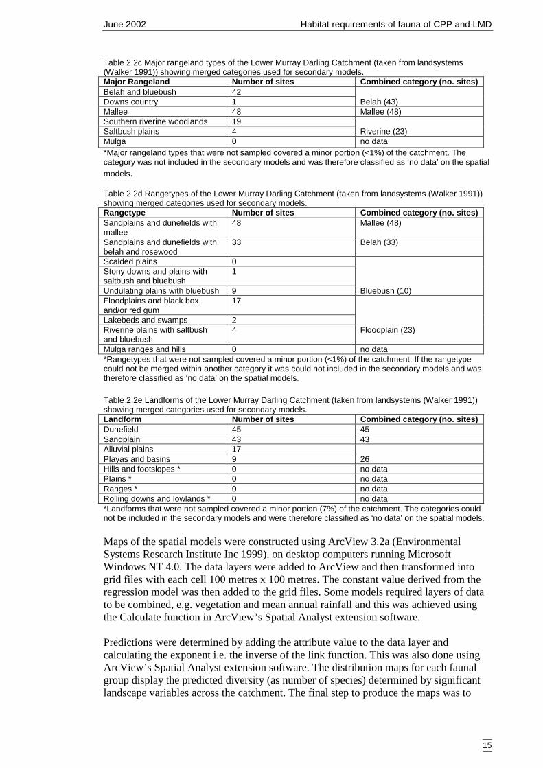
15
Table 2.2c Major rangeland types of the Lower Murray Darling Catchment (taken from landsystems(Walker 1991)) showing merged categories used for secondary models.Major Rangeland Number of sites Combined category (no. sites)Belah and bluebush 42Downs country 1 Belah (43)Mallee 48 Mallee (48)Southern riverine woodlands 19Saltbush plains 4 Riverine (23)Mulga 0 no data*Major rangeland types that were not sampled covered a minor portion (<1%) of the catchment. Thecategory was not included in the secondary models and was therefore classified as ‘no data’ on the spatialmodels.
Table 2.2d Rangetypes of the Lower Murray Darling Catchment (taken from landsystems (Walker 1991))showing merged categories used for secondary models.Rangetype Number of sites Combined category (no. sites)Sandplains and dunefields withmallee
48 Mallee (48)
Sandplains and dunefields withbelah and rosewood
33 Belah (33)
Scalded plains 0Stony downs and plains withsaltbush and bluebush
1
Undulating plains with bluebush 9 Bluebush (10)Floodplains and black boxand/or red gum
17
Lakebeds and swamps 2Riverine plains with saltbushand bluebush
4 Floodplain (23)
Mulga ranges and hills 0 no data*Rangetypes that were not sampled covered a minor portion (<1%) of the catchment. If the rangetypecould not be merged within another category it was could not included in the secondary models and wastherefore classified as ‘no data’ on the spatial models.
Table 2.2e Landforms of the Lower Murray Darling Catchment (taken from landsystems (Walker 1991))showing merged categories used for secondary models.Landform Number of sites Combined category (no. sites)Dunefield 45 45Sandplain 43 43Alluvial plains 17Playas and basins 9 26Hills and footslopes * 0 no dataPlains * 0 no dataRanges * 0 no dataRolling downs and lowlands * 0 no data*Landforms that were not sampled covered a minor portion (7%) of the catchment. The categories couldnot be included in the secondary models and were therefore classified as ‘no data’ on the spatial models.
Maps of the spatial models were constructed using ArcView 3.2a (EnvironmentalSystems Research Institute Inc 1999), on desktop computers running MicrosoftWindows NT 4.0. The data layers were added to ArcView and then transformed intogrid files with each cell 100 metres x 100 metres. The constant value derived from theregression model was then added to the grid files. Some models required layers of datato be combined, e.g. vegetation and mean annual rainfall and this was achieved usingthe Calculate function in ArcView’s Spatial Analyst extension software.
Predictions were determined by adding the attribute value to the data layer andcalculating the exponent i.e. the inverse of the link function. This was also done usingArcView’s Spatial Analyst extension software. The distribution maps for each faunalgroup display the predicted diversity (as number of species) determined by significantlandscape variables across the catchment. The final step to produce the maps was to
June 2002 Habitat requirements of fauna of CPP and LMD
16
overlay the GIS coverage of areas approved for clearing for dryland cultivation orhorticulture (DLWC GIS 2001). This would highlight portions of the catchment thatwere no longer available for consideration for conservation.
Table 2.2f Vegetation types of Lower Murray Darling Catchment used for secondary models.Original vegetation type (vegetationcommunity (6))
Number ofsites
Mergedvegetation type(vegetationcommunity (4))
Number of sites formerged vegetationcommunities
Belah (Casuarina pauper) woodland 40Chenopod (Maireana pyramidata andM. sedifolia) shrubland
20
Riverine (black box (Eucalyptuslargiflorens)) woodlands
16
Mallee (Eucalyptus dumosa, E. gracilisand E. oleosa) over mixed chenopod(Maireana spp)
9
Sand dune mallee (Eucalyptus socialis,E. costata and E. leptophylla) withmixed shrubs and spinifex (Triodiascariosa)
25
Sandplain mallee (Eucalyptus socialis,E. dumosa and E. gracilis) with mixedshrubs and spinifex (Triodia scariosa)
4
Mallee 38
May 2002 Habitat requirements of fauna of CPP and LMD
17
May 2002 Habitat requirements of fauna of CPP and LMD
18
May 2002 Habitat requirements of fauna of CPP and LMD
19
May 2002 Habitat requirements of fauna of CPP and LMD
20
May 2002 Habitat requirements of fauna of CPP and LMD
21
May 2002 Habitat requirements of fauna of CPP and LMD
22
May 2002 Habitat requirements of fauna of CPP and LMD
23
May 2002 Habitat requirements of fauna of CPP and LMD
24
3 RESULTS
3.1 VEGETATION
3.1.1 Classification and ordinationSpecies that occurred more than once across the study site were analysed with the finaldata set comprised 255 perennial species from 194 sites.
Site classificationSite classification revealed five broad communities, or groups, (ANOSIM, pseudoF=1.40, p<0.001) (Appendix E) representing a gradient from east to west across thestudy region. These were:� mulga (Acacia aneura ssp) shrublands in the east (Group I, 19 sites);� a large complex group of sites of various vegetation communities from across the
study area (Group II, 79 sites);� ridge sites located in the east (Group III, 12 sites); and� mallee (Eucalyptus spp) communities (Group IV, 44 sites) from the west and� belah (Casuarina spp) woodlands (Group V, 40 sites) also located in the west of the
region.
Following a separate classification, Group II split into five sub-groups (ANOSIM,pseudo F=1.38, p<0.001) (Appendix F). These were identified as belah (Casuarinacristata) sites located in the eastern portion of the region (Group IIa, 15 sites), riverinesites located in the east (Group IIb, six sites), white cypress pine (Callitrisglaucophylla) sites on rocky ridges in the east (Group IIc, 18 sites), chenopod (mixedMaireana spp) shrubland sites, some with a belah (Casuarina pauper) overstorey, in thewest of the region (Group IId, 27 sites), and a fifth group of riverine sites located in thewest (Group IIe, 13 sites).
Species classificationSpecies classification also revealed a gradient across the study region from east to westwith 12 final groups defined. The primary split in the species classification separated thedata into three main groups based on species abundance (ANOSIM, pseudo F=2.04,p<0.001). These were:� Species that were recorded as present only and restricted to the eastern portion of
the study area formed one block which was located at the top of the dendogram(Appendix G, Group 1, 56 species). These were sites located on the CobarPeneplain.
� A large second group, located in the middle of the dendogram, represented thosespecies that occurred in higher densities across the study region (Appendix G,Group 2, 150 species).
May 2002 Habitat requirements of fauna of CPP and LMD
25
� A third block located at the bottom of the dendogram of present only species fromthe west of the study area, namely the Lower Murray Darling Catchment (AppendixG, Group 3, 49 species).
A second classification was required to clarify the sub-groups within Group 2. Fourgroups were apparent (ANOSIM, pseudo F=1.16, p<0.001) (Appendix H) with Groups2a and 2b requiring a third classification. Group 2a separated into five sub-groups(ANOSIM, pseudo F=1.77, p<0.001) (Appendix I) and Group 2b into three sub-groups(ANOSIM, pseudo F=1.12, p<0.001) (Appendix J).
The sub-groups of Group 2a are numbered 1-5 (Appendix I). Sub-group 2a1 (32species) consisted of species that occurred across all communities but which had higherdensities in the western portion of the region. Sub-group 2a2 (8 species) consisted ofridge species that occurred exclusively within the eastern portion of the region on theCobar Peneplain. Species in sub-group 2a3 (4 species) were recorded predominantly aspresent only and mainly in the east. Subgroups 2a4 (7 species) and 2a5 (7 species) werecomposed of riverine species confined to the Lower Murray Darling Catchment.
Sub-group 2b1 (30 species) was a collection of ridge species recorded in the east of theregion (Appendix J). Sub-group 2b2 (21 species) was also from the east and representedthe widespread white cypress pine (Callitris glaucophylla), bimble box (Eucalyptuspopulnea subsp bimbil) and red box (E. intertexta) communities. The belah (Casuarinacristata and C. pauper) woodland species of sub-group 2b3 (14 species) were recordedacross the study region.
Group 2c (22 species) from the second classification were species occurring with mallee(Eucalyptus spp)/spinifex (Triodia scariosa) communities and located primarily in thewest of the study region (Appendix H). The final species group, Group 2d, was a smallcollection (five species) of infrequently encountered species in the east of the region(Appendix H).
EvaluationThe final stage of the classification process was construction of a two-way tableillustrating the distribution of species across sites. Closer inspection revealed thatunderstorey or sub-dominant overstorey species were responsible for some sites beingplaced within groups that did not correspond to the dominant species recorded at thesite. Eight sites were then re-located to the group that more accurately reflected thedominant species on site. The amended distribution of sites is shown in the two-waytable (Appendix K).
The communities were defined by the abundance of common overstorey species andadditional co-dominants. Equally significant were the widespread and less frequentunderstorey species. Descriptions of these final nine groups are below and followdendogram order.
Descriptions of the nine vegetation types
1. Mulga (Acacia anuera var. latifolia, A. aneura var. aneura) shrublands +/-ironwood (A. excelsa) over mixed shrubs.
No. sites in group: 19 sites (19 from the Cobar Peneplain, 0 from Lower Murray DarlingCatchment).
May 2002 Habitat requirements of fauna of CPP and LMD
26
Total number of species in group: 96
Principal species with cover/abundance score (18): mulga (Acacia aneura var. latifolia, A. aneura var.aneura), ironwood (A. excelsa), punty bush (Senna artemisioides subsp filifolia), silver cassia (S.artemisioides subsp artemisioides), narrow-leaf hopbush (Dodonaea viscosa subsp angustissima),green hopbush (D. petiolaris), western boobialla (Myoporum montanum), woollybutt (Eragrostiseriopoda), supplejack (Ventilago viminalis), turpentine (Eremophila sturtii), emubush (E. longifolia),crimson foxtail (Ptilotus atriplicifolius var. atriplicifolius), sand spurge (Phyllanthus fuernrohrii),beefwood (Grevillea striata), bloodwood (Corymbia tumescens), mountain wanderrie grass (Eriachnemucronata) and five-minute grass (Tripogon loliiformis).
2. Belah (Casuarina cristata) woodland +/- leopardwood (Flindersia maculosa)over wilga (Geijera parviflora), turpentine (Eremophila sturtii) and budda(Eremophila mitchellii) shrubs.
No. sites in group: 15 sites (15 from the Cobar Peneplain, 0 from Lower Murray DarlingCatchment).
Total number of species in group: 69
Principal species with cover/abundance score (9): belah (Casuarina cristata), leopardwood(Flindersia maculosa), wilga (Geijera parviflora), turpentine (Eremophila sturtii), budda (E.mitchellii), warrior bush (Apophyllum anomalum), grey copperburr (Sclerolaena diacantha),galvanized burr (S. birchii) and speargrass species (Austrostipa spp).
3. Bimble box (Eucalyptus populnea subsp bimbil) woodland +/- red gum (E.camaldulensis) over slender bamboo grass (Austrostipa verticillata) tussockgrassland.
No. sites in group: 6 sites (6 from the Cobar Peneplain, 0 from Lower Murray Darling Catchment).
Total number of species in group: 53
Principal species with cover/abundance score (6): bimble box (Eucalyptus populnea subsp. bimbil),red gum (E. camaldulensis), coolibah apple (Angophora melanoxylon), sticky wallaby-bush(Beyeria viscosa), slender bamboo grass (Austrostipa verticillata) and windmill grass (Chloristruncata).
4. White cypress pine (Callitris glaucophylla) woodland +/- currawang (Acaciadoratoxylon) shrub.
No. sites in group: 16 sites (16 from the Cobar Peneplain, 0 from Lower Murray DarlingCatchment).
Total number of species in group: 81
Principal species with cover/abundance score (7): white cypress pine (Callitris glaucophylla),currawang (Acacia doratoxylon), mountain wanderrie grass (Eriachne mucronata), inland wongavine (Pandorea pandorana), crimson foxtail (Ptilotus atriplicifolius var. atriplicifolius), no. 9wiregrass (Aristida jerichoensis) and rough speargrass (Austrostipa scabra subsp. scabra).
5. Bluebush (Maireana pyramidata +/- M. sedifolia) shrubland +/- belah(Casuarina pauper) and rosewood (Alectryon oleifolius) over copperburr(Sclerolaena obliquicuspis and S. diacantha).
No. sites in group: 24 sites (0 from the Cobar Peneplain, 24 from Lower Murray DarlingCatchment).
Total number of species in group: 74
May 2002 Habitat requirements of fauna of CPP and LMD
27
Principal species with cover/abundance score (9): black bluebush (Maireana pyramidata), pearlbluebush (M. sedifolia), M. appressa, belah (Casuarina pauper), rosewood (Alectryon oleifolius),limestone copperburr (Sclerolaena obliquicuspis), pale poverty-bush (S. divaricata) andspeargrasses (Austrostipa nitida and A. nodosa).
6. Black box (Eucalyptus largiflorens) woodland +/- river red gum (E.camaldulensis) over lignum (Muehlenbeckia florulenta).
No. sites in group: 17 sites (1 from the Cobar Peneplain, 16 from Lower Murray DarlingCatchment).
Total number of species in group: 55
Principal species with cover/abundance score (16) black box (Eucalyptus largiflorens), river redgum (E. camaldulensis), lignum (Muehlenbeckia florulenta), river cooba (Acacia stenophylla),lippia (Phyla nodiflora), nitre goosefoot (Chenopodium nitrariaceum), warrego summer-grass(Paspalidium jubiflorum), spreading saltbush (Atriplex limbata), small saltbush (A. eardleyae),eastern flat-top saltbush (A. lindleyi), slender-fruit saltbush (A. leptocarpa), streaked poverty-bush(Sclerolaena tricuspis), roly-poly (S. muricata var. muricata), spear-fruit copperburr (S.patenticuspis), star copperburr (S. stelligera) and red copperburr (S. calcarata).
7. White cypress pine (Callitris glaucophylla)+/- bimble box (E. populnea subspbimbil) and red box (E. intertexta) woodland over wilga (Geijera parviflora)shrub.
No. sites in group: 12 sites (12 from the Cobar Peneplain, 0 from Lower Murray DarlingCatchment).
Total number of species in group: 105
Principal species with cover/abundance score (22) white cypress pine (Callitris glaucophylla),bimble box (E. populnea subsp bimbil), red box (E. intertexta), grey mallee (E. morrisii), kurrajong(Brachychiton populneus), quinine bush (Alstonia constricta), wilga (Geijera parviflora), inlandwonga vine (Pandorea pandorana), budda (Eremophila mitchellii), tar bush (E. glabra), stickywallaby-bush (Beyeria viscosa), dead finish (Acacia tetragonophylla), Deane’s wattle (A. deanei),broad-leaf hopbush (Dodonaea viscosa subsp. spatulata), climbing saltbush (Einadia nutans), longgreybeard grass (Amphipogon caricinus var. caricinus), yellow burr-daisy (Calotis lappulacea),speargrass species (Austrostipa spp), mulga grass (Thyridiolepis mitchelliana), mountain wanderriegrass (Eriachne mucronata) and other grasses (Eragrostis spp and Aristida spp).
8. Mallee (Eucalyptus socialis and E. dumosa +/- E. gracilis, leptophylla andcostata) over mixed shrubs and spinifex (Triodia scariosa).
No. sites in group: 45 sites (11 from the Cobar Peneplain, 34 from Lower Murray DarlingCatchment).
Total number of species in group: 135
Principal species with cover/abundance score (19): pointed mallee (Eucalyptus socialis), congoomallee (E. dumosa), yorrell (E. gracilis), narrow-leaf red mallee (E. leptophylla), lerp mallee (E.costata), mallee cypress pine (Callitris verrucosa), spinifex (Triodia scariosa), needle wattle(Acacia rigens), Wilhelm's wattle (A. wilhelmiana), umbrella bush (A. ligulata), broad-leafedhopbush (Dodonaea viscosa subsp. angustissima), Mueller's daisy-bush (Olearia muelleri), greycassia (Senna artemisioides subsp. petiolaris), erect mallee bluebush (Maireana pentatropis), cactuspea (Bossiaea walkeri), stiff western rosemary (Westringia rigida), spreading flax-lily (Dianellarevoluta), felted nightshade (Solanum coactiliferum) and grey copperburr (Sclerolaena diacantha).
May 2002 Habitat requirements of fauna of CPP and LMD
28
9. Belah (Casuarina pauper) woodlands over rosewood (Alectryon oleifolius), wilga(Geijera parviflora) and mixed shrubs.
No. sites in group: 40 sites (0 from the Cobar Peneplain, 40 from Lower Murray DarlingCatchment).
Total number of species in group: 79
Principal species with cover/abundance score (19): belah (Casuarina pauper), rosewood (Alectryonoleifolius), wilga (Geijera parviflora), sugarwood (Myoporum platycarpum subsp. platycarpum),leafless cherry (Exocarpos aphyllus), spine bush (Acacia colletioides), showy daisy-bush (Oleariapimeleoides), Mueller's daisy-bush (O. muelleri), dense cassia (Senna artemisioides nothosubsp.coriacea), satiny bluebush (Maireana georgei), erect mallee bluebush (M. pentatropis), woolly-fruited copperburr (M. sclerolaenoides), black bluebush (M. pyramidata), ruby saltbush (Enchylaenatomentosa), cannon-ball (Dissocarpus paradoxus), limestone copperburr (Sclerolaenaobliquicuspis), grey copperburr (S. diacantha), cottony saltbush (Chenopodium curvispicatum) andbitter saltbush (Atriplex stipitata).
OrdinationOrdination of the vegetation data required four dimensions in order to reduce the stressto an acceptable level (stress = 0.16). As distance between site groups is an indication ofthe degree of similarity, sites (or groups) that are further apart in the ordination spaceare more dissimilar, while those close together are more similar (Figure 3.1a).Significant plant species that were most highly correlated to the ordination space wereplotted as vectors and assisted in describing which species were associated with eachordination axis. Several groups overlapped, particularly near the centre of the ordinationspace but other groups were more clearly separated.
Ordination axis 1 poorly differentiated classification groups but Group VIII was evidentin the upper right of the ordination space where mallee (Eucalyptus socialis and E.dumosa) and spinifex (Triodia scariosa) were best fitted to the ordination space.Ordination axis 2 separated the Cobar Peneplain sites of Group VII from Group VIIIwith wilga (Geijera parviflora) and white cypress pine (Callitris glaucophylla) fittedalong axis 2 in the region of Group VII. Ordination axis 3 clearly separated the CobarPeneplain sites of Group I from the Lower Murray Darling sites of Group IX with belah(Casuarina pauper), rosewood (Alectryon oleifolius) and wilga (Geijera parviflora)vectors fitted to the ordination in the region of Group IX. The fourth ordination axisseparated the Cobar Peneplain sites of Group II from Group VIII with mallee species(Eucalyptus socialis and E. dumosa) and white cypress pine (Callitris glaucophylla)vectors fitted in the region of Group VIII in the upper right section.
Table 3.1a Plant species correlated with the ordination space on the basis of a Monte-Carlo test.Species abbreviation Species name Correlation (r)
Alecolei Alectryon oleifolius 0.76Atristip Aristida stipitata 0.61Callglau Callitris glaucophylla 0.65Casupaup Casuarina pauper 0.81Cheisieb Cheilanthes sieberi spp. sieberi 0.68Enchtome Enchylaena tomentosa 0.69Eucadumo Eucalyptus dumosa 0.77Eucasoci Eucalyptus socialis 0.73Geijparv Geijera parviflora 0.71Mairpent Maireana pentatropis 0.65Trioscar Triodia scariosa 0.74*p<0.05, **p<0.01, **p<0.001
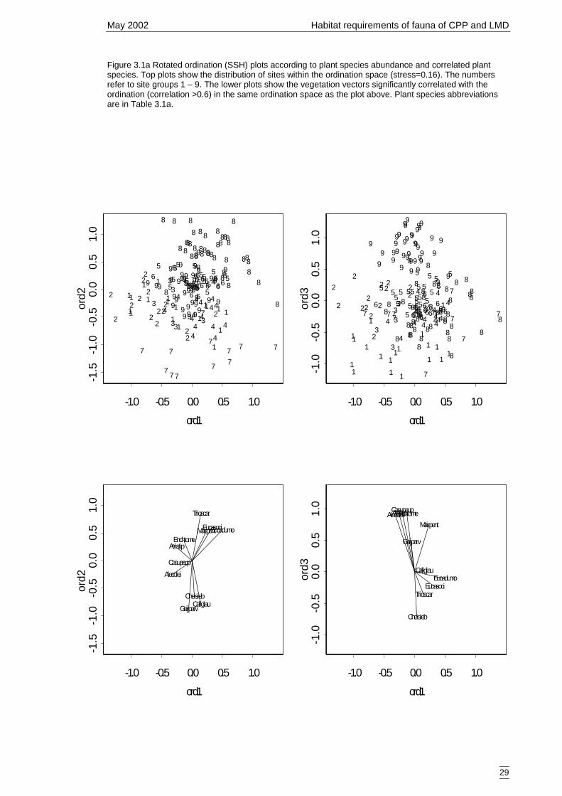
May 2002 Habitat requirements of fauna of CPP and LMD
29
Figure 3.1a Rotated ordination (SSH) plots according to plant species abundance and correlated plantspecies. Top plots show the distribution of sites within the ordination space (stress=0.16). The numbersrefer to site groups 1 – 9. The lower plots show the vegetation vectors significantly correlated with theordination (correlation >0.6) in the same ordination space as the plot above. Plant species abbreviationsare in Table 3.1a.
-1.0 -0.5 0.0 0.5 1.0ord1
-1.5
-1.0
-0.5
0.0
0.5
1.0
ord2
1
211
11
131
1
1
11
1
34
44
42
14
88
4
4
4
4
4
2
2
5
7
77
8
7
8
7
8
7
3
2
7
7
2
7
7
2
3
2
2 32
7
7
41
1
22
2 6
1
3
12
1
1
8
24
8
8
4
8
8
444
9
8
8
9
8
5
99
88
9
5
5
9 8
9
8
95
8
9
8
9
9
8
5 99
8
55
999
66
8
95
9
9 5
8
9 95
88
6 966
8
8
559
99
8 8
55
99
8
8
995
65 44
99
8 8
6 6
5
9
8
8
595
8
88
98
56 8
8
65 695 5
8
8
9
9
9
8
9
9 56 5
5
-1.0 -0.5 0.0 0.5 1.0ord1
-1.5
-1.0
-0.5
0.0
0.5
1.0
ord2
CallglauCheisieb
EucadumoEucasoci
Trioscar
Atristip
CasupaupAlecolei
Geijparv
EnchtomeMairpent
-1.0 -0.5 0.0 0.5 1.0ord1
-1.0
-0.5
0.0
0.5
1.0
ord3
1
2
1
11
1
1
3
1 1
11 1
13
444
42
1 4
88
4 4
44
4
22
57 7 7
8
78
7
8
73
2
7
7
2
7
7
232
2
32 77
4
11
222
6
1
3
1
2
1
1
8
2
4 8
8
4
8
8444
9
8
8
9
8
5
9
9
8
8
95
5
9
8
9
8
9
5 8
9 89
9
8
5
9
9
85
5
99
9
6
68
9
5
9
9
5
8
9 9
5
8
86
9
668
8
55
9
9
9
8
85
5
99
8
8
9
9
565
44
9
9
88
66
5
9
88
5
9
588
8
9
856
88
65
6
9
5 5
8
8
99
9
8
9
95
6 5
5
-1.0 -0.5 0.0 0.5 1.0ord1
-1.0
-0.5
0.0
0.5
1.0
ord3
Callglau
Cheisieb
EucadumoEucasoci
Trioscar
AtristipCasupaupAlecolei
Geijparv
EnchtomeMairpent
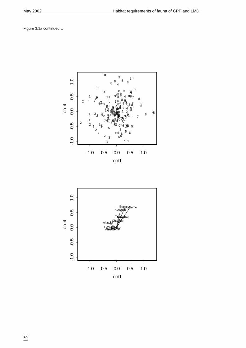
May 2002 Habitat requirements of fauna of CPP and LMD
30
Figure 3.1a continued…
-1.0 -0.5 0.0 0.5 1.0ord1
-1.0
-0.5
0.0
0.5
1.0
ord4
1
2
11
11
1
31
1
1
1
11
3
4
4
4
4
2
1
4
88
4
4
4
4
4
22
57
7
7
8
7
8
7
8
7
32
7
7
2
7
72
3
2
2
3
2 77
4
1
12
2
2
6
1 3
12
1
1
8
2
4
88
4
8
8
4
44
9
8
89
8
5 99
8
8
95
5
9
8
9
895
8
9
8
9
9
85
9
9
8
5599 9
6
6
8
9
5
9
9
5
8
9
9
5
8
8
6
9
66
88
5
59
99
8
8
559
9
8
8
99
5
6
5
44
998
8
66
5
9
88
5
95
88
8
9
8
5
6
88
6
5
6
95
5
8
8
9
99
8
9
9
565 5
-1.0 -0.5 0.0 0.5 1.0
ord1
-1.0
-0.5
0.0
0.5
1.0
ord4
Callglau
Cheisieb
EucadumoEucasoci
Trioscar
AtristipCasupaup
Alecolei
GeijparvEnchtome
Mairpent
May 2002 Habitat requirements of fauna of CPP and LMD
31
3.2 BIRDS
3.2.1 Classification and ordinationNinety-four species from 192 sites were used in the analysis. These were species thatoccurred more than once across the study area but excluded larger mobile species suchas raptors, parrots and nocturnal species. Presence/absence data was analysed.
Site classificationSites were classified to identify groups of sites with similar bird distributions. Theclassification revealed six groups (ANOSIM, pseudo F=1.46, p<0.001) (Appendix M)and no further investigation into individual site groups was required.
Species classificationSpecies were classified to identify groups of species with similar geographicaldistributions. Species classification revealed a total of 10 groups from primary andsubsequent analysis. The initial cut of the dendogram produced four groups (ANOSIM,pseudo F=1.77, p<0.001) (Appendix N) based on frequency. The least encounteredspecies were at the lower end of the dendogram, consisting of Groups 2 – 4. Group 1,located at the top of the dendogram, was composed of the more frequently encounteredspecies.
Classification of Group 1 split the species into five sub-groups, Groups 1a – 1e(ANOSIM, pseudo F=1.56, p<0.001) (Appendix O), according to frequency within eachsite group and the degree of geographical spread. Group 1d required further clarificationand split into two groups (ANOSIM, pseudo F=1.41, p<0.001) (Appendix P). This splitseparated the widespread species from those requiring a more restricted habitat.
Group 3 secondary classification revealed two groups based on species association withriverine wetland habitats (ANOSIM, pseudo F=2.02, p<0.001) (Appendix Q).
EvaluationThe final stage of the classification process was construction of a two-way tableillustrating the distribution of species across sites (Appendix R). Site groups were testedagainst floristic data to determine the associated vegetation communities to help withnaming the bird species groups. Table 3.2a summarises these results.
OrdinationThe results from the principal axis correlation did not reveal any species highly linearlycorrelated to vegetation gradients (r<0.5, p > 0.05). Bubble plots of the abundance ofeach species group against each ordination axis did not reveal any trends in association,except for Group 6 (mallee (Eucalyptus spp) bird species) which showed a trend ofincreasing abundance in the upper half of the ordination space for ordination axes 2 and4. This corresponds to the region where mallee (Eucalyptus spp) and white cypress pine(Callitris glaucophylla) were best fitted.
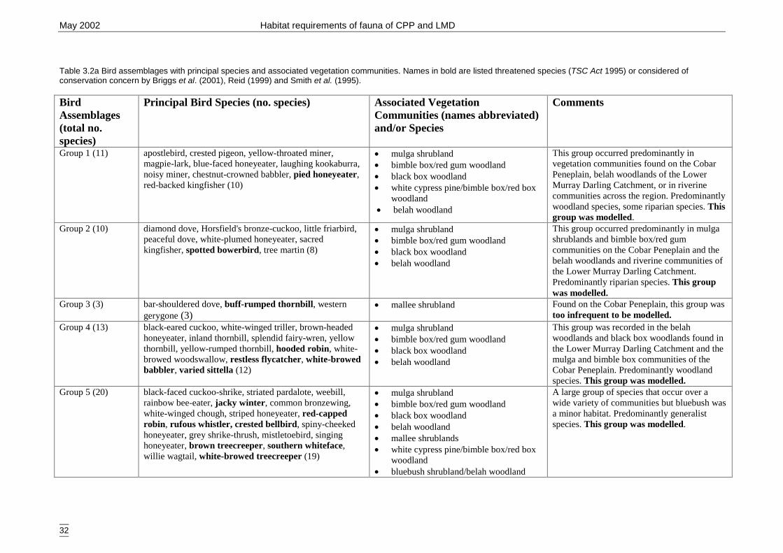
May 2002 Habitat requirements of fauna of CPP and LMD
32
Table 3.2a Bird assemblages with principal species and associated vegetation communities. Names in bold are listed threatened species (TSC Act 1995) or considered ofconservation concern by Briggs et al. (2001), Reid (1999) and Smith et al. (1995).
BirdAssemblages(total no.species)
Principal Bird Species (no. species) Associated VegetationCommunities (names abbreviated)and/or Species
Comments
Group 1 (11) apostlebird, crested pigeon, yellow-throated miner,magpie-lark, blue-faced honeyeater, laughing kookaburra,noisy miner, chestnut-crowned babbler, pied honeyeater,red-backed kingfisher (10)
� mulga shrubland� bimble box/red gum woodland� black box woodland� white cypress pine/bimble box/red box
woodland� belah woodland
This group occurred predominantly invegetation communities found on the CobarPeneplain, belah woodlands of the LowerMurray Darling Catchment, or in riverinecommunities across the region. Predominantlywoodland species, some riparian species. Thisgroup was modelled.
Group 2 (10) diamond dove, Horsfield's bronze-cuckoo, little friarbird,peaceful dove, white-plumed honeyeater, sacredkingfisher, spotted bowerbird, tree martin (8)
� mulga shrubland� bimble box/red gum woodland� black box woodland� belah woodland
This group occurred predominantly in mulgashrublands and bimble box/red gumcommunities on the Cobar Peneplain and thebelah woodlands and riverine communities ofthe Lower Murray Darling Catchment.Predominantly riparian species. This groupwas modelled.
Group 3 (3) bar-shouldered dove, buff-rumped thornbill, westerngerygone (3)
� mallee shrubland Found on the Cobar Peneplain, this group wastoo infrequent to be modelled.
Group 4 (13) black-eared cuckoo, white-winged triller, brown-headedhoneyeater, inland thornbill, splendid fairy-wren, yellowthornbill, yellow-rumped thornbill, hooded robin, white-browed woodswallow, restless flycatcher, white-browedbabbler, varied sittella (12)
� mulga shrubland� bimble box/red gum woodland� black box woodland� belah woodland
This group was recorded in the belahwoodlands and black box woodlands found inthe Lower Murray Darling Catchment and themulga and bimble box communities of theCobar Peneplain. Predominantly woodlandspecies. This group was modelled.
Group 5 (20) black-faced cuckoo-shrike, striated pardalote, weebill,rainbow bee-eater, jacky winter, common bronzewing,white-winged chough, striped honeyeater, red-cappedrobin, rufous whistler, crested bellbird, spiny-cheekedhoneyeater, grey shrike-thrush, mistletoebird, singinghoneyeater, brown treecreeper, southern whiteface,willie wagtail, white-browed treecreeper (19)
� mulga shrubland� bimble box/red gum woodland� black box woodland� belah woodland� mallee shrublands� white cypress pine/bimble box/red box
woodland� bluebush shrubland/belah woodland
A large group of species that occur over awide variety of communities but bluebush wasa minor habitat. Predominantly generalistspecies. This group was modelled.
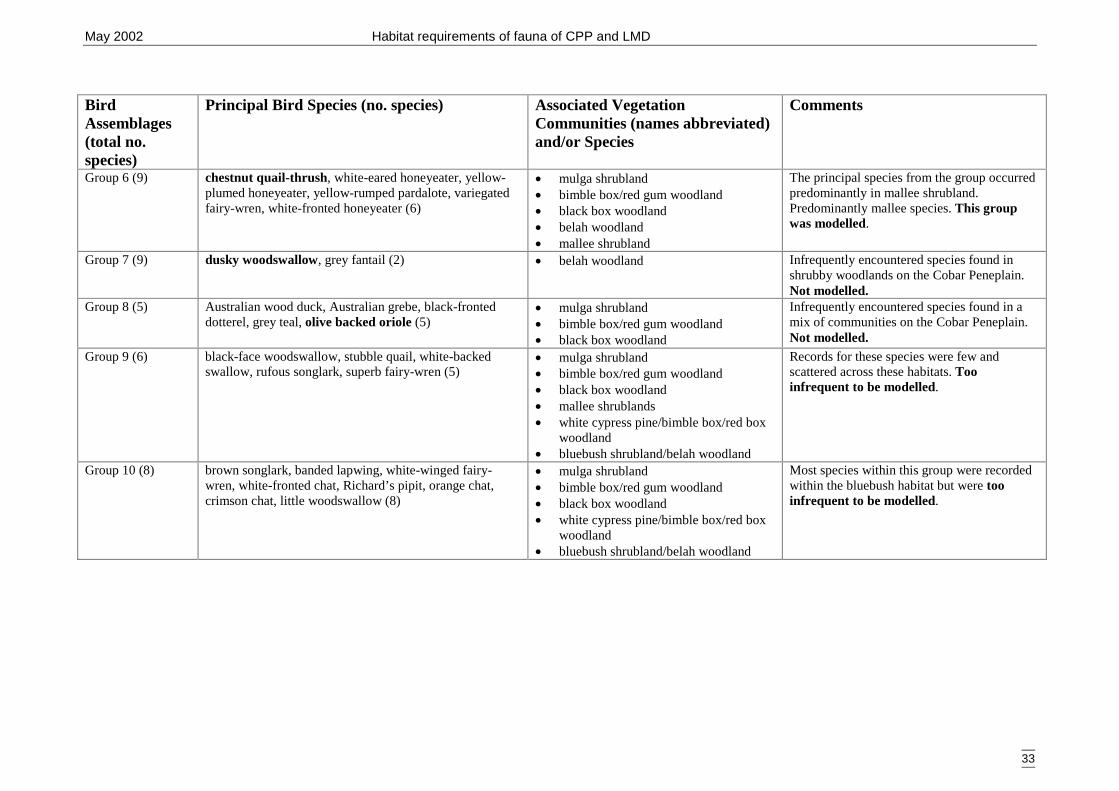
May 2002 Habitat requirements of fauna of CPP and LMD
33
BirdAssemblages(total no.species)
Principal Bird Species (no. species) Associated VegetationCommunities (names abbreviated)and/or Species
Comments
Group 6 (9) chestnut quail-thrush, white-eared honeyeater, yellow-plumed honeyeater, yellow-rumped pardalote, variegatedfairy-wren, white-fronted honeyeater (6)
� mulga shrubland� bimble box/red gum woodland� black box woodland� belah woodland� mallee shrubland
The principal species from the group occurredpredominantly in mallee shrubland.Predominantly mallee species. This groupwas modelled.
Group 7 (9) dusky woodswallow, grey fantail (2) � belah woodland Infrequently encountered species found inshrubby woodlands on the Cobar Peneplain.Not modelled.
Group 8 (5) Australian wood duck, Australian grebe, black-fronteddotterel, grey teal, olive backed oriole (5)
� mulga shrubland� bimble box/red gum woodland� black box woodland
Infrequently encountered species found in amix of communities on the Cobar Peneplain.Not modelled.
Group 9 (6) black-face woodswallow, stubble quail, white-backedswallow, rufous songlark, superb fairy-wren (5)
� mulga shrubland� bimble box/red gum woodland� black box woodland� mallee shrublands� white cypress pine/bimble box/red box
woodland� bluebush shrubland/belah woodland
Records for these species were few andscattered across these habitats. Tooinfrequent to be modelled.
Group 10 (8) brown songlark, banded lapwing, white-winged fairy-wren, white-fronted chat, Richard’s pipit, orange chat,crimson chat, little woodswallow (8)
� mulga shrubland� bimble box/red gum woodland� black box woodland� white cypress pine/bimble box/red box
woodland� bluebush shrubland/belah woodland
Most species within this group were recordedwithin the bluebush habitat but were tooinfrequent to be modelled.
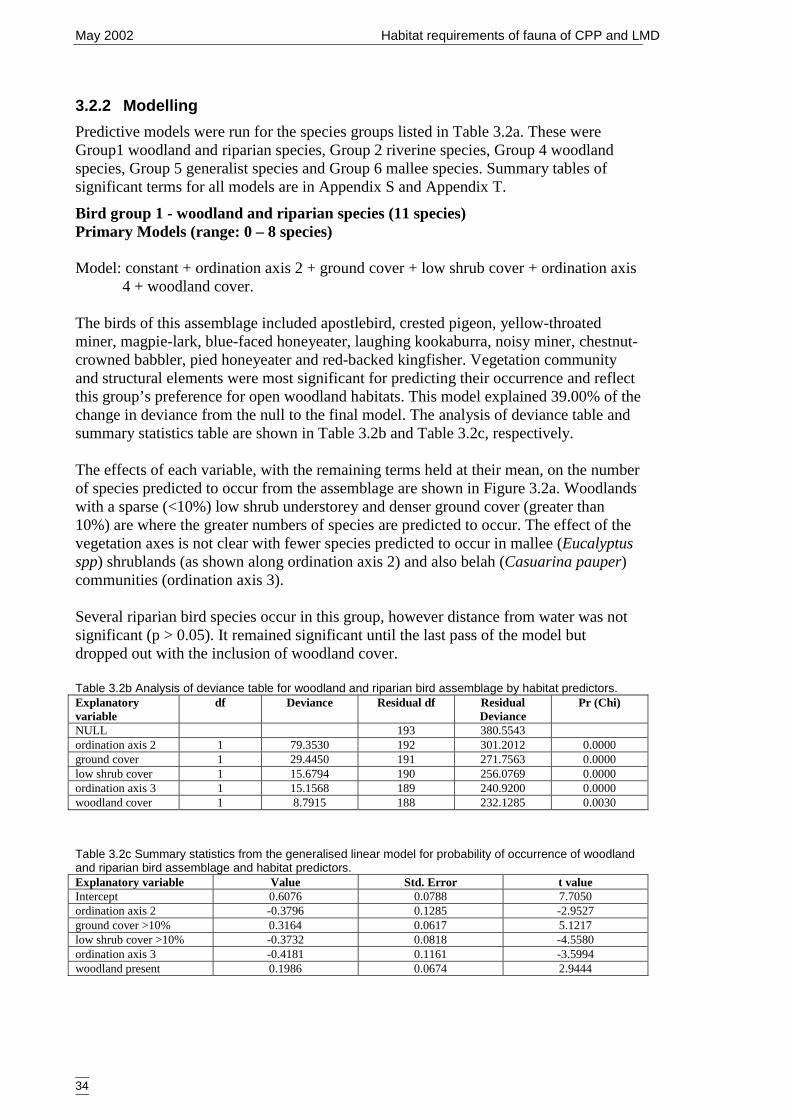
May 2002 Habitat requirements of fauna of CPP and LMD
34
3.2.2 ModellingPredictive models were run for the species groups listed in Table 3.2a. These wereGroup1 woodland and riparian species, Group 2 riverine species, Group 4 woodlandspecies, Group 5 generalist species and Group 6 mallee species. Summary tables ofsignificant terms for all models are in Appendix S and Appendix T.
Bird group 1 - woodland and riparian species (11 species)Primary Models (range: 0 – 8 species)
Model: constant + ordination axis 2 + ground cover + low shrub cover + ordination axis4 + woodland cover.
The birds of this assemblage included apostlebird, crested pigeon, yellow-throatedminer, magpie-lark, blue-faced honeyeater, laughing kookaburra, noisy miner, chestnut-crowned babbler, pied honeyeater and red-backed kingfisher. Vegetation communityand structural elements were most significant for predicting their occurrence and reflectthis group’s preference for open woodland habitats. This model explained 39.00% of thechange in deviance from the null to the final model. The analysis of deviance table andsummary statistics table are shown in Table 3.2b and Table 3.2c, respectively.
The effects of each variable, with the remaining terms held at their mean, on the numberof species predicted to occur from the assemblage are shown in Figure 3.2a. Woodlandswith a sparse (<10%) low shrub understorey and denser ground cover (greater than10%) are where the greater numbers of species are predicted to occur. The effect of thevegetation axes is not clear with fewer species predicted to occur in mallee (Eucalyptusspp) shrublands (as shown along ordination axis 2) and also belah (Casuarina pauper)communities (ordination axis 3).
Several riparian bird species occur in this group, however distance from water was notsignificant (p > 0.05). It remained significant until the last pass of the model butdropped out with the inclusion of woodland cover.
Table 3.2b Analysis of deviance table for woodland and riparian bird assemblage by habitat predictors.Explanatoryvariable
df Deviance Residual df ResidualDeviance
Pr (Chi)
NULL 193 380.5543ordination axis 2 1 79.3530 192 301.2012 0.0000ground cover 1 29.4450 191 271.7563 0.0000low shrub cover 1 15.6794 190 256.0769 0.0000ordination axis 3 1 15.1568 189 240.9200 0.0000woodland cover 1 8.7915 188 232.1285 0.0030
Table 3.2c Summary statistics from the generalised linear model for probability of occurrence of woodlandand riparian bird assemblage and habitat predictors.Explanatory variable Value Std. Error t valueIntercept 0.6076 0.0788 7.7050ordination axis 2 -0.3796 0.1285 -2.9527ground cover >10% 0.3164 0.0617 5.1217low shrub cover >10% -0.3732 0.0818 -4.5580ordination axis 3 -0.4181 0.1161 -3.5994woodland present 0.1986 0.0674 2.9444
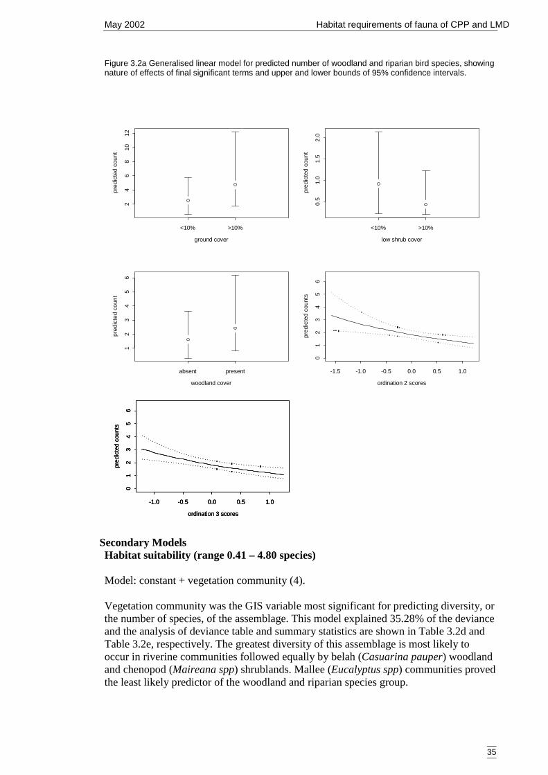
May 2002 Habitat requirements of fauna of CPP and LMD
35
Figure 3.2a Generalised linear model for predicted number of woodland and riparian bird species, showingnature of effects of final significant terms and upper and lower bounds of 95% confidence intervals.
Secondary ModelsHabitat suitability (range 0.41 – 4.80 species)
Model: constant + vegetation community (4).
Vegetation community was the GIS variable most significant for predicting diversity, orthe number of species, of the assemblage. This model explained 35.28% of the devianceand the analysis of deviance table and summary statistics are shown in Table 3.2d andTable 3.2e, respectively. The greatest diversity of this assemblage is most likely tooccur in riverine communities followed equally by belah (Casuarina pauper) woodlandand chenopod (Maireana spp) shrublands. Mallee (Eucalyptus spp) communities provedthe least likely predictor of the woodland and riparian species group.
ordination 3 scores
pred
icte
d co
unts
-1.0 -0.5 0.0 0.5 1.0
01
23
45
6
ordination 3 scores
pred
icte
d co
unts
-1.0 -0.5 0.0 0.5 1.0
01
23
45
6
ordination 3 scores
pred
icte
d co
unts
-1.0 -0.5 0.0 0.5 1.0
01
23
45
6
ground cover
pred
icte
d co
unt
24
68
1012
<10% >10%
low shrub cover
pred
icte
d co
unt
0.5
1.0
1.5
2.0
<10% >10%
woodland cover
pred
icte
d co
unt
12
34
56
absent present
ordination 2 scores
pred
icte
d co
unts
-1.5 -1.0 -0.5 0.0 0.5 1.0
01
23
45
6

May 2002 Habitat requirements of fauna of CPP and LMD
36
Table 3.2d Analysis of deviance table for woodland and riparian bird assemblage by GIS predictors.Explanatory variable df Deviance Residual df Residual
DeviancePr (Chi)
NULL 113 50.9574vegetation community (4) 2 17.9802 111 32.9772 0.0001
Table 3.2e Summary statistics for predicted abundance of species from woodland and riparian birdassemblage and GIS predictors.Explanatory variable Value Std. Error t valueIntercept 0.3718 0.1071 3.4685riverine 0.4671 0.1962 2.3809mallee -0.5476 0.2070 -2.6450
Spatial representationThe spatial interpolation of the secondary model maps the predicted diversity of theassemblage at a landscape scale. In the current model, the spatial representation isprimarily the vegetation coverage and predicts that greater diversity will be restricted tothe riverine corridors and riverine communities (2.31 species) and fewest in mallee(Eucalyptus spp) communities (0.84 species). Belah (Casuarina pauper) woodland andchenopod (Maireana spp) shrublands were predicted to be more diverse than mallee(Eucalyptus spp) communities but less diverse than riverine communities (1.45 species)(Appendix U). The predicted preference for riverine areas reflects these communitiessignificance for providing the suitable habitat defined by the micro-scale, on-sitevariables. Thus, it is predicted that riverine communities will provide the vegetationcommunity and structural cover required for the woodland and riparian assemblage.
Count (range: 0 – 8 species)
Model: constant + vegetation group (4).
The model tests the recorded number of species from the species group against GISvariables. The final model identifies vegetation community as the only significant term,explaining 26.43% of the deviance. The deviance and the analysis of deviance table andsummary statistics are shown in Table 3.2f and Table 3.2g.
Table 3.2f Analysis of deviance table for woodland and riparian bird assemblage by GIS predictors.Explanatory variable df Deviance Residual df Residual
DeviancePr
(Chi)NULL 113 252.9577vegetation community (4) 2 66.8580 111 186.0996 0.000
Table 3.2g Summary statistics for count of species from woodland and riparian bird assemblage and GISpredictors.Explanatory variable Value Std. Error t valueIntercept 0.3600 0.1075 3.3469riverine 0.8927 0.1715 5.2043mallee -1.1068 0.2561 -4.3212
Spatial representationThe spatial interpolation of the model testing the recorded number of species is similarto the previous one testing predicted values and is also a representation of the vegetationcoverage. Similarly, more species will occur along the riverine corridors (3.5 species)with fewest in mallee (Eucalyptus spp) communities (0.47 species). Species diversity inbelah (Casuarina pauper) woodland and chenopod (Maireana spp) shrublands waspredicted to be midway between these two values (1.43 species) (Appendix V).Although the same landscape variable was identified, the diversity values predicted
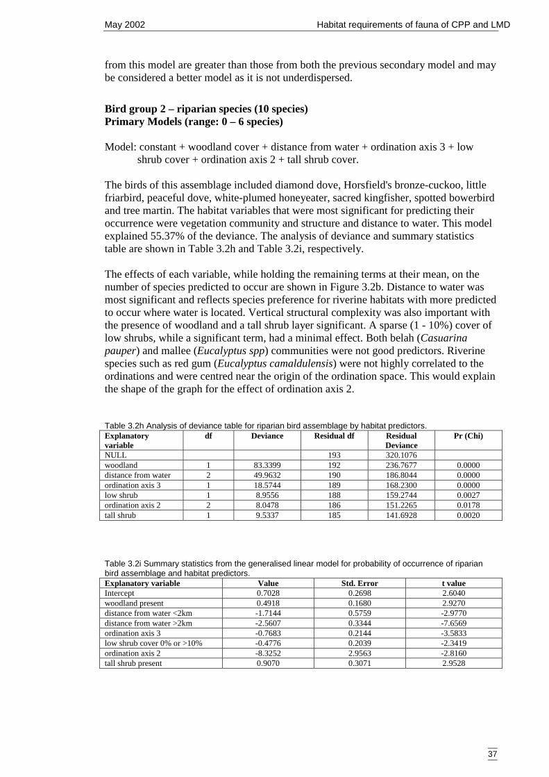
May 2002 Habitat requirements of fauna of CPP and LMD
37
from this model are greater than those from both the previous secondary model and maybe considered a better model as it is not underdispersed.
Bird group 2 – riparian species (10 species)Primary Models (range: 0 – 6 species)
Model: constant + woodland cover + distance from water + ordination axis 3 + lowshrub cover + ordination axis 2 + tall shrub cover.
The birds of this assemblage included diamond dove, Horsfield's bronze-cuckoo, littlefriarbird, peaceful dove, white-plumed honeyeater, sacred kingfisher, spotted bowerbirdand tree martin. The habitat variables that were most significant for predicting theiroccurrence were vegetation community and structure and distance to water. This modelexplained 55.37% of the deviance. The analysis of deviance and summary statisticstable are shown in Table 3.2h and Table 3.2i, respectively.
The effects of each variable, while holding the remaining terms at their mean, on thenumber of species predicted to occur are shown in Figure 3.2b. Distance to water wasmost significant and reflects species preference for riverine habitats with more predictedto occur where water is located. Vertical structural complexity was also important withthe presence of woodland and a tall shrub layer significant. A sparse (1 - 10%) cover oflow shrubs, while a significant term, had a minimal effect. Both belah (Casuarinapauper) and mallee (Eucalyptus spp) communities were not good predictors. Riverinespecies such as red gum (Eucalyptus camaldulensis) were not highly correlated to theordinations and were centred near the origin of the ordination space. This would explainthe shape of the graph for the effect of ordination axis 2.
Table 3.2h Analysis of deviance table for riparian bird assemblage by habitat predictors.Explanatoryvariable
df Deviance Residual df ResidualDeviance
Pr (Chi)
NULL 193 320.1076woodland 1 83.3399 192 236.7677 0.0000distance from water 2 49.9632 190 186.8044 0.0000ordination axis 3 1 18.5744 189 168.2300 0.0000low shrub 1 8.9556 188 159.2744 0.0027ordination axis 2 2 8.0478 186 151.2265 0.0178tall shrub 1 9.5337 185 141.6928 0.0020
Table 3.2i Summary statistics from the generalised linear model for probability of occurrence of riparianbird assemblage and habitat predictors.Explanatory variable Value Std. Error t valueIntercept 0.7028 0.2698 2.6040woodland present 0.4918 0.1680 2.9270distance from water <2km -1.7144 0.5759 -2.9770distance from water >2km -2.5607 0.3344 -7.6569ordination axis 3 -0.7683 0.2144 -3.5833low shrub cover 0% or >10% -0.4776 0.2039 -2.3419ordination axis 2 -8.3252 2.9563 -2.8160tall shrub present 0.9070 0.3071 2.9528
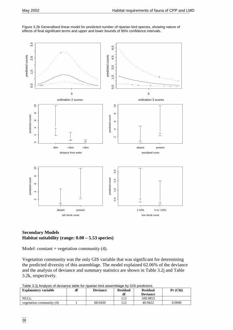
May 2002 Habitat requirements of fauna of CPP and LMD
38
Figure 3.2b Generalised linear model for predicted number of riparian bird species, showing nature ofeffects of final significant terms and upper and lower bounds of 95% confidence intervals.
Secondary ModelsHabitat suitability (range: 0.00 – 5.53 species)
Model: constant + vegetation community (4).
Vegetation community was the only GIS variable that was significant for determiningthe predicted diversity of this assemblage. The model explained 62.06% of the devianceand the analysis of deviance and summary statistics are shown in Table 3.2j and Table3.2k, respectively.
Table 3.2j Analysis of deviance table for riparian bird assemblage by GIS predictors.Explanatory variable df Deviance Residual
dfResidualDeviance
Pr (Chi)
NULL 113 108.9853vegetation community (4) 1 68.0430 112 40.9422 0.0000
distance from water
pred
icte
d co
unts
02
46
810
0km <2km >2km
woodland cover
pred
icte
d co
unt
24
68
10
absent present
tall shrub cover
pred
icte
d co
unt
24
68
10
absent present
low shrub cover
pred
icte
d co
unt
0.5
1.0
1.5
2.0
1-10% 0 or >10%
ordination 2 scores
pred
icte
d co
unts
0
0.0
1.0
2.0
3.0
ordination 3 scores
pred
icte
d co
unts
0
0.0
1.5
3.0
4.5
6.0
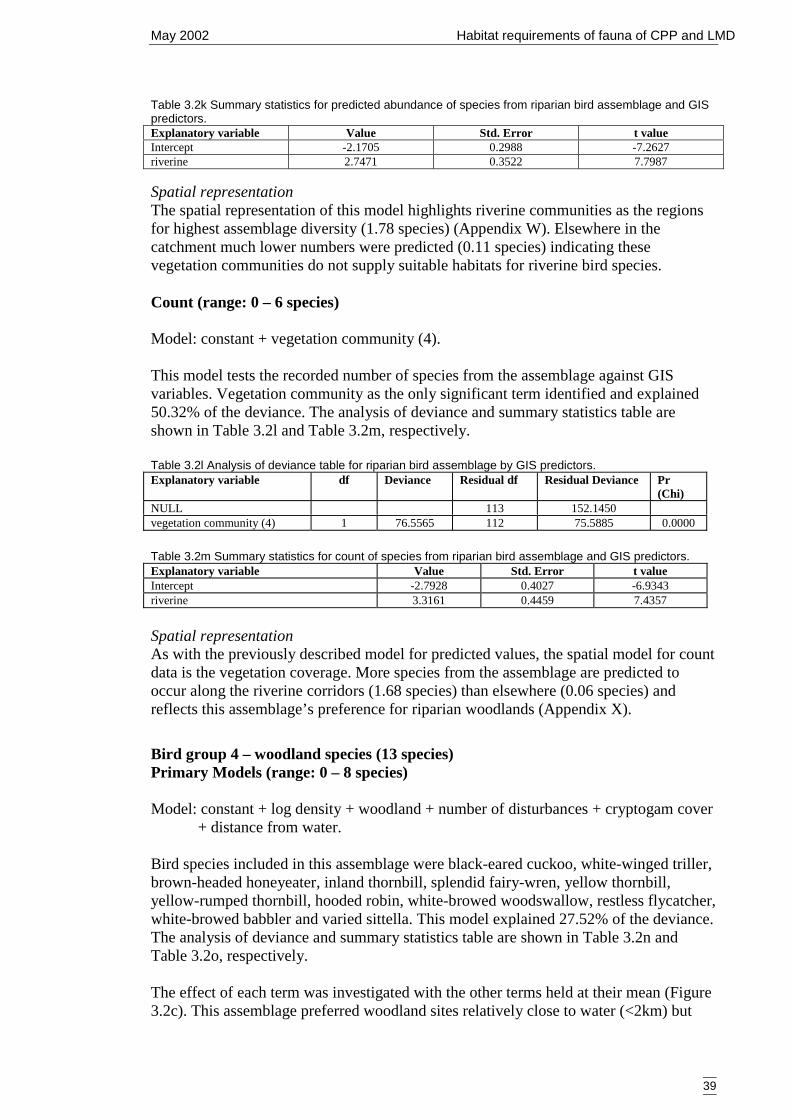
May 2002 Habitat requirements of fauna of CPP and LMD
39
Table 3.2k Summary statistics for predicted abundance of species from riparian bird assemblage and GISpredictors.Explanatory variable Value Std. Error t valueIntercept -2.1705 0.2988 -7.2627riverine 2.7471 0.3522 7.7987
Spatial representationThe spatial representation of this model highlights riverine communities as the regionsfor highest assemblage diversity (1.78 species) (Appendix W). Elsewhere in thecatchment much lower numbers were predicted (0.11 species) indicating thesevegetation communities do not supply suitable habitats for riverine bird species.
Count (range: 0 – 6 species)
Model: constant + vegetation community (4).
This model tests the recorded number of species from the assemblage against GISvariables. Vegetation community as the only significant term identified and explained50.32% of the deviance. The analysis of deviance and summary statistics table areshown in Table 3.2l and Table 3.2m, respectively.
Table 3.2l Analysis of deviance table for riparian bird assemblage by GIS predictors.Explanatory variable df Deviance Residual df Residual Deviance Pr
(Chi)NULL 113 152.1450vegetation community (4) 1 76.5565 112 75.5885 0.0000
Table 3.2m Summary statistics for count of species from riparian bird assemblage and GIS predictors.Explanatory variable Value Std. Error t valueIntercept -2.7928 0.4027 -6.9343riverine 3.3161 0.4459 7.4357
Spatial representationAs with the previously described model for predicted values, the spatial model for countdata is the vegetation coverage. More species from the assemblage are predicted tooccur along the riverine corridors (1.68 species) than elsewhere (0.06 species) andreflects this assemblage’s preference for riparian woodlands (Appendix X).
Bird group 4 – woodland species (13 species)Primary Models (range: 0 – 8 species)
Model: constant + log density + woodland + number of disturbances + cryptogam cover+ distance from water.
Bird species included in this assemblage were black-eared cuckoo, white-winged triller,brown-headed honeyeater, inland thornbill, splendid fairy-wren, yellow thornbill,yellow-rumped thornbill, hooded robin, white-browed woodswallow, restless flycatcher,white-browed babbler and varied sittella. This model explained 27.52% of the deviance.The analysis of deviance and summary statistics table are shown in Table 3.2n andTable 3.2o, respectively.
The effect of each term was investigated with the other terms held at their mean (Figure3.2c). This assemblage preferred woodland sites relatively close to water (<2km) but
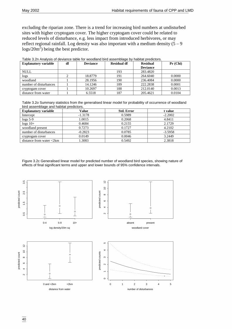
May 2002 Habitat requirements of fauna of CPP and LMD
40
excluding the riparian zone. There is a trend for increasing bird numbers at undisturbedsites with higher cryptogam cover. The higher cryptogam cover could be related toreduced levels of disturbance, e.g. less impact from introduced herbivores, or mayreflect regional rainfall. Log density was also important with a medium density (5 – 9logs/20m2) being the best predictor.
Table 3.2n Analysis of deviance table for woodland bird assemblage by habitat predictors.Explanatory variable df Deviance Residual df Residual
DeviancePr (Chi)
NULL 193 283.4820logs 2 18.8779 191 264.6040 0.0000woodland 1 28.1956 190 236.4084 0.0000number of disturbances 1 14.1246 189 222.2838 0.0001cryptogam cover 1 10.2697 188 212.0140 0.0013distance from water 1 6.5518 187 205.4621 0.0104
Table 3.2o Summary statistics from the generalised linear model for probability of occurrence of woodlandbird assemblage and habitat predictors.Explanatory variable Value Std. Error t valueIntercept -1.3178 0.5989 -2.2002logs 5-9 1.0015 0.2068 4.8411logs 10+ 0.4684 0.2155 2.1729woodland present 0.7273 0.1727 4.2102number of disturbances -0.2823 0.0785 -3.5958cryptogam cover 0.0149 0.0046 3.2449distance from water <2km 1.3083 0.5492 2.3818
Figure 3.2c Generalised linear model for predicted number of woodland bird species, showing nature ofeffects of final significant terms and upper and lower bounds of 95% confidence intervals.
log density/20m sq
pred
icte
d co
unt
0.5
1.5
2.5
3.5
0-4 5-9 10+
woodland cover
pred
icte
d co
unt
24
68
1012
absent present
distance from water
pred
icte
d co
unt
24
68
1012
0 and >2km <2km
number of disturbances
pred
icte
d co
unts
0 1 2 3 4 5
01
23
45
May 2002 Habitat requirements of fauna of CPP and LMD
41
Secondary ModelsHabitat suitability (range: 0.08 – 5.52 species)
Model: constant + vegetation community (4) + mean annual rainfall.
This model explained 28.61% of the deviance. The analysis of deviance and summarystatistics table are shown in Table 3.2p and Table 3.2q, respectively. Greater assemblagediversity was predicted by vegetation community and mean annual rainfall, specificallybelah (Casuarina pauper) woodlands and riverine communities and higher rainfall.
Table 3.2p Analysis of deviance table for woodland bird assemblage by GIS predictors.Explanatory variable df Deviance Residual df Residual
DeviancePr (Chi)
NULL 113 58.0230vegetation community (4) 2 11.3329 111 46.6901 0.0034mean annual rainfall 1 5.2693 110 41.4208 0.0217
Table 3.2q Summary statistics for predicted abundance of species from woodland bird assemblage andGIS predictors.Explanatory variable Value Std. Error t valueIntercept -2.3530 1.1558 -2.0357chenopod vegetation community -0.9891 0.3442 -2.8736mallee vegetation community -0.3393 0.2044 -1.6599mean annual rainfall 0.0101 0.0044 2.2927
Spatial representationA strong north-west to south-east gradient is evident in the spatial interpolation of thismodel. Numbers were predicted to be lowest in the north-west (<0.50 species) wherelow rainfall and chenopod (Maireana spp) shrublands dominate. In the south-east,where belah (Casuarina pauper) woodlands, riverine communities and higher rainfalloccur, greater diversity was predicted (maximum 2.50 species) (Appendix Y).
Count (range: 0 - 8 species)
Model: constant + vegetation community (4) + mean annual rainfall.
This model accounted for 16.27% of the deviance with vegetation community and meanannual rainfall predicting the occurrence of woodland species. The analysis of devianceand summary statistics table are shown in Table 3.2r and Table 3.2s, respectively.
cryptogam cover
pred
icte
d co
unts
0 20 40 60 80
02
46
8
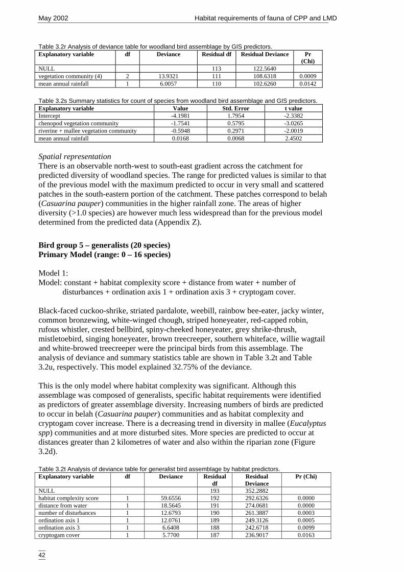
May 2002 Habitat requirements of fauna of CPP and LMD
42
Table 3.2r Analysis of deviance table for woodland bird assemblage by GIS predictors.Explanatory variable df Deviance Residual df Residual Deviance Pr
(Chi)NULL 113 122.5640vegetation community (4) 2 13.9321 111 108.6318 0.0009mean annual rainfall 1 6.0057 110 102.6260 0.0142
Table 3.2s Summary statistics for count of species from woodland bird assemblage and GIS predictors.Explanatory variable Value Std. Error t valueIntercept -4.1981 1.7954 -2.3382chenopod vegetation community -1.7541 0.5795 -3.0265riverine + mallee vegetation community -0.5948 0.2971 -2.0019mean annual rainfall 0.0168 0.0068 2.4502
Spatial representationThere is an observable north-west to south-east gradient across the catchment forpredicted diversity of woodland species. The range for predicted values is similar to thatof the previous model with the maximum predicted to occur in very small and scatteredpatches in the south-eastern portion of the catchment. These patches correspond to belah(Casuarina pauper) communities in the higher rainfall zone. The areas of higherdiversity (>1.0 species) are however much less widespread than for the previous modeldetermined from the predicted data (Appendix Z).
Bird group 5 – generalists (20 species)Primary Model (range: 0 – 16 species)
Model 1:Model: constant + habitat complexity score + distance from water + number of
disturbances + ordination axis 1 + ordination axis 3 + cryptogam cover.
Black-faced cuckoo-shrike, striated pardalote, weebill, rainbow bee-eater, jacky winter,common bronzewing, white-winged chough, striped honeyeater, red-capped robin,rufous whistler, crested bellbird, spiny-cheeked honeyeater, grey shrike-thrush,mistletoebird, singing honeyeater, brown treecreeper, southern whiteface, willie wagtailand white-browed treecreeper were the principal birds from this assemblage. Theanalysis of deviance and summary statistics table are shown in Table 3.2t and Table3.2u, respectively. This model explained 32.75% of the deviance.
This is the only model where habitat complexity was significant. Although thisassemblage was composed of generalists, specific habitat requirements were identifiedas predictors of greater assemblage diversity. Increasing numbers of birds are predictedto occur in belah (Casuarina pauper) communities and as habitat complexity andcryptogam cover increase. There is a decreasing trend in diversity in mallee (Eucalyptusspp) communities and at more disturbed sites. More species are predicted to occur atdistances greater than 2 kilometres of water and also within the riparian zone (Figure3.2d).
Table 3.2t Analysis of deviance table for generalist bird assemblage by habitat predictors.Explanatory variable df Deviance Residual
dfResidualDeviance
Pr (Chi)
NULL 193 352.2882habitat complexity score 1 59.6556 192 292.6326 0.0000distance from water 1 18.5645 191 274.0681 0.0000number of disturbances 1 12.6793 190 261.3887 0.0003ordination axis 1 1 12.0761 189 249.3126 0.0005ordination axis 3 1 6.6408 188 242.6718 0.0099cryptogam cover 1 5.7700 187 236.9017 0.0163
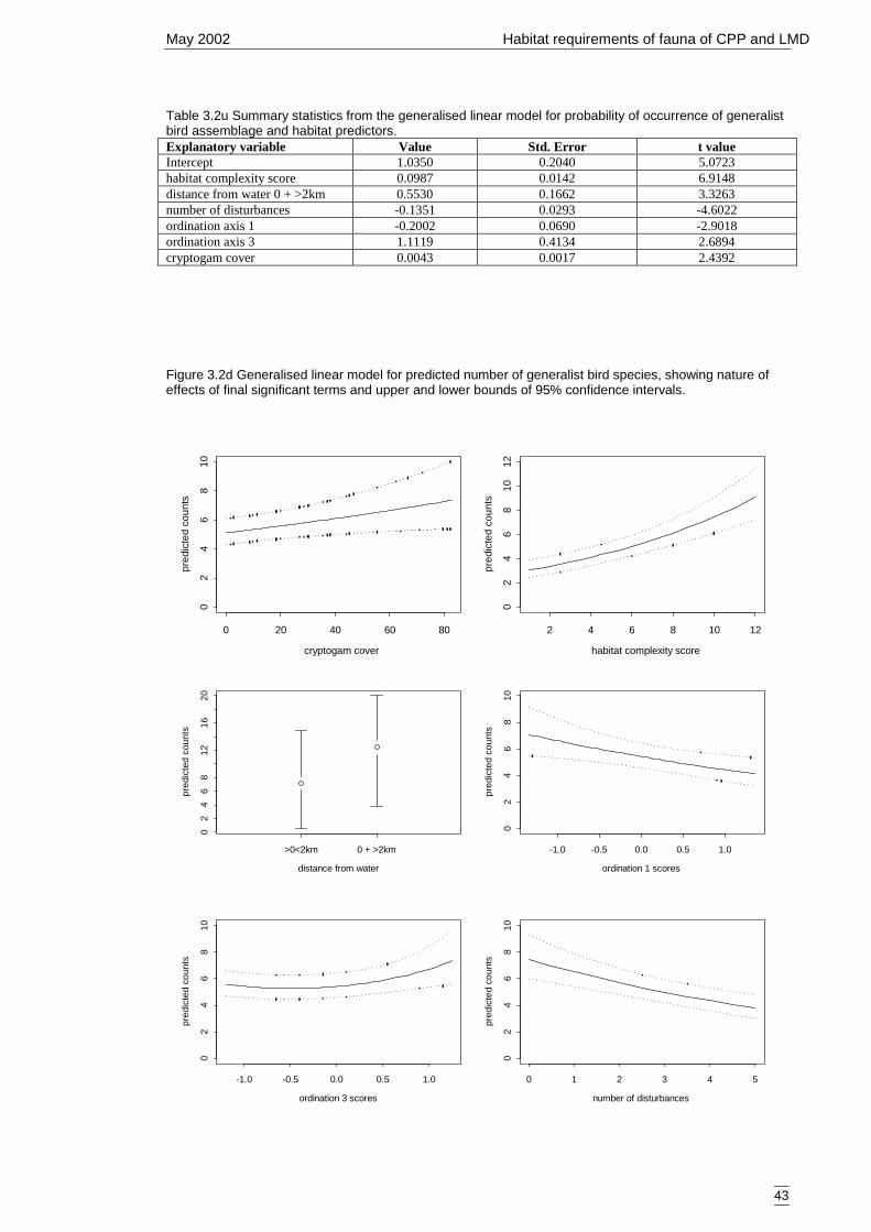
May 2002 Habitat requirements of fauna of CPP and LMD
43
Table 3.2u Summary statistics from the generalised linear model for probability of occurrence of generalistbird assemblage and habitat predictors.Explanatory variable Value Std. Error t valueIntercept 1.0350 0.2040 5.0723habitat complexity score 0.0987 0.0142 6.9148distance from water 0 + >2km 0.5530 0.1662 3.3263number of disturbances -0.1351 0.0293 -4.6022ordination axis 1 -0.2002 0.0690 -2.9018ordination axis 3 1.1119 0.4134 2.6894cryptogam cover 0.0043 0.0017 2.4392
Figure 3.2d Generalised linear model for predicted number of generalist bird species, showing nature ofeffects of final significant terms and upper and lower bounds of 95% confidence intervals.
distance from water
pred
icte
d co
unts
02
46
812
1620
>0<2km 0 + >2km
ordination 1 scores
pred
icte
d co
unts
-1.0 -0.5 0.0 0.5 1.0
02
46
810
ordination 3 scores
pred
icte
d co
unts
-1.0 -0.5 0.0 0.5 1.0
02
46
810
number of disturbances
pred
icte
d co
unts
0 1 2 3 4 5
02
46
810
cryptogam cover
pred
icte
d co
unts
0 20 40 60 80
02
46
810
habitat complexity score
pred
icte
d co
unts
2 4 6 8 10 12
02
46
810
12
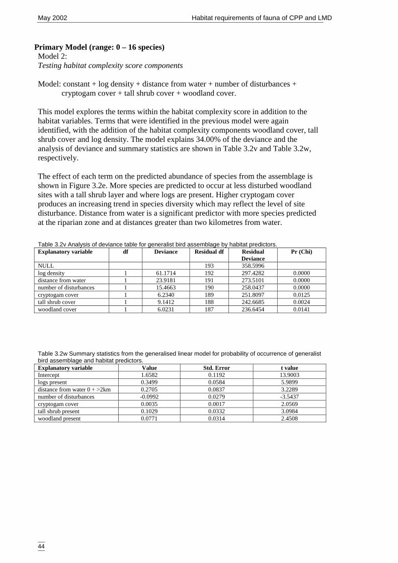
May 2002 Habitat requirements of fauna of CPP and LMD
44
Primary Model (range: 0 – 16 species)Model 2:Testing habitat complexity score components
Model: constant + log density + distance from water + number of disturbances +cryptogam cover + tall shrub cover + woodland cover.
This model explores the terms within the habitat complexity score in addition to thehabitat variables. Terms that were identified in the previous model were againidentified, with the addition of the habitat complexity components woodland cover, tallshrub cover and log density. The model explains 34.00% of the deviance and theanalysis of deviance and summary statistics are shown in Table 3.2v and Table 3.2w,respectively.
The effect of each term on the predicted abundance of species from the assemblage isshown in Figure 3.2e. More species are predicted to occur at less disturbed woodlandsites with a tall shrub layer and where logs are present. Higher cryptogam coverproduces an increasing trend in species diversity which may reflect the level of sitedisturbance. Distance from water is a significant predictor with more species predictedat the riparian zone and at distances greater than two kilometres from water.
Table 3.2v Analysis of deviance table for generalist bird assemblage by habitat predictors.Explanatory variable df Deviance Residual df Residual
DeviancePr (Chi)
NULL 193 358.5996log density 1 61.1714 192 297.4282 0.0000distance from water 1 23.9181 191 273.5101 0.0000number of disturbances 1 15.4663 190 258.0437 0.0000cryptogam cover 1 6.2340 189 251.8097 0.0125tall shrub cover 1 9.1412 188 242.6685 0.0024woodland cover 1 6.0231 187 236.6454 0.0141
Table 3.2w Summary statistics from the generalised linear model for probability of occurrence of generalistbird assemblage and habitat predictors.Explanatory variable Value Std. Error t valueIntercept 1.6582 0.1192 13.9003logs present 0.3499 0.0584 5.9899distance from water 0 + >2km 0.2705 0.0837 3.2289number of disturbances -0.0992 0.0279 -3.5437cryptogam cover 0.0035 0.0017 2.0569tall shrub present 0.1029 0.0332 3.0984woodland present 0.0771 0.0314 2.4508
May 2002 Habitat requirements of fauna of CPP and LMD
45
Figure 3.2e Generalised linear model for predicted number of generalist bird species, showing nature ofeffects of final significant terms, including habitat complexity score components and upper and lowerbounds of 95% confidence intervals.
Secondary ModelsHabitat suitability (range: 1.98– 15.89 species)Model 1Testing habitat complexity score
Model: constant + vegetation community (4).
Vegetation community was the only significant term in determining the predictednumber of species from the assemblage. This model explained 41.29% of the deviance.The analysis of deviance and summary statistics table are shown in Table 3.2x andTable 3.2y, respectively.
log density/20m sq
pred
icte
d co
unts
24
68
1216
20
absent present
distance from water
pred
icte
d co
unts
02
46
812
1620
>0<2km 0 + >2km
tall shrub cover
pred
icte
d co
unts
13
57
911
13
absent present
woodland cover
pred
icte
d co
unts
13
57
911
13
absent present
number of disturbances
pred
icte
d co
unts
0 1 2 3 4 5
02
46
810
cryptogam cover
pred
icte
d co
unts
0 20 40 60 80
02
46
810
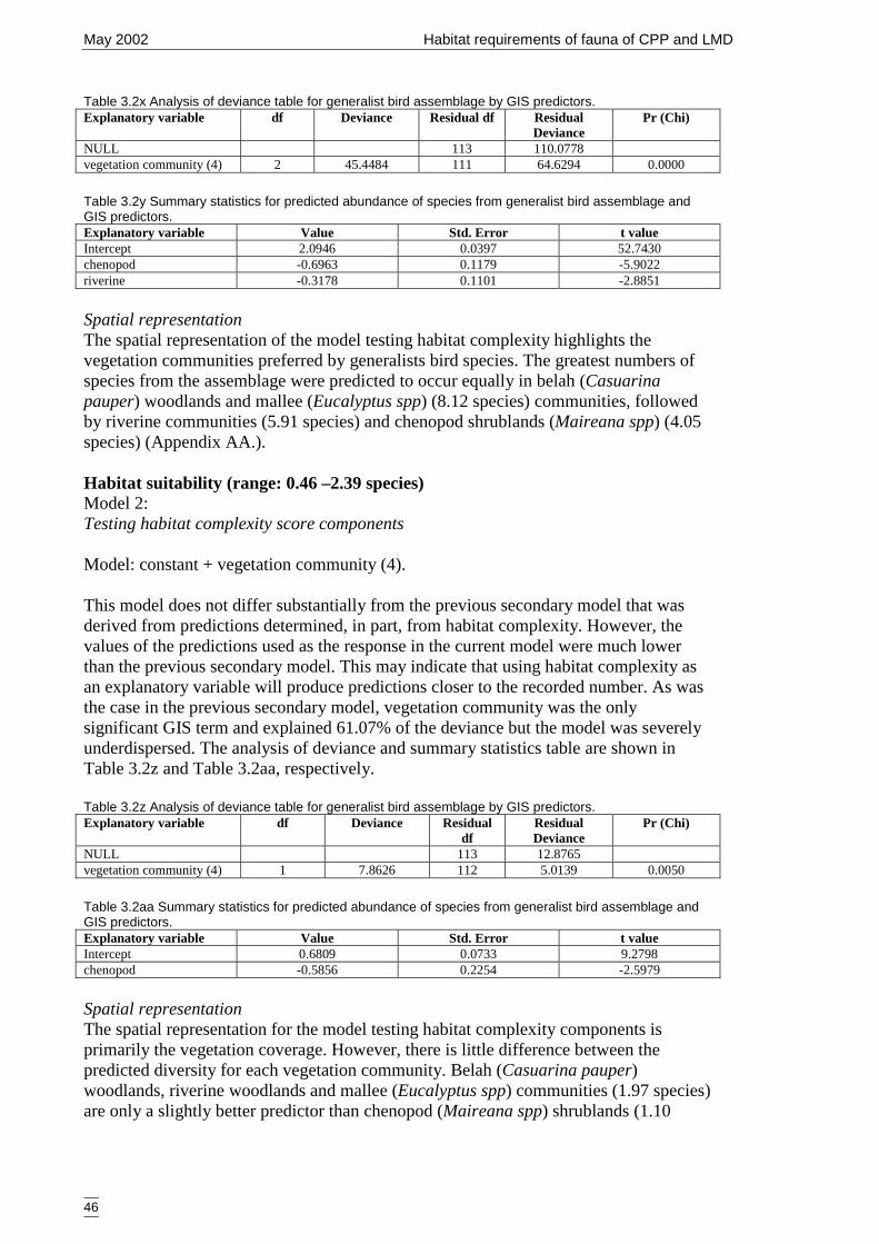
May 2002 Habitat requirements of fauna of CPP and LMD
46
Table 3.2x Analysis of deviance table for generalist bird assemblage by GIS predictors.Explanatory variable df Deviance Residual df Residual
DeviancePr (Chi)
NULL 113 110.0778vegetation community (4) 2 45.4484 111 64.6294 0.0000
Table 3.2y Summary statistics for predicted abundance of species from generalist bird assemblage andGIS predictors.Explanatory variable Value Std. Error t valueIntercept 2.0946 0.0397 52.7430chenopod -0.6963 0.1179 -5.9022riverine -0.3178 0.1101 -2.8851
Spatial representationThe spatial representation of the model testing habitat complexity highlights thevegetation communities preferred by generalists bird species. The greatest numbers ofspecies from the assemblage were predicted to occur equally in belah (Casuarinapauper) woodlands and mallee (Eucalyptus spp) (8.12 species) communities, followedby riverine communities (5.91 species) and chenopod shrublands (Maireana spp) (4.05species) (Appendix AA.).
Habitat suitability (range: 0.46 –2.39 species)Model 2:Testing habitat complexity score components
Model: constant + vegetation community (4).
This model does not differ substantially from the previous secondary model that wasderived from predictions determined, in part, from habitat complexity. However, thevalues of the predictions used as the response in the current model were much lowerthan the previous secondary model. This may indicate that using habitat complexity asan explanatory variable will produce predictions closer to the recorded number. As wasthe case in the previous secondary model, vegetation community was the onlysignificant GIS term and explained 61.07% of the deviance but the model was severelyunderdispersed. The analysis of deviance and summary statistics table are shown inTable 3.2z and Table 3.2aa, respectively.
Table 3.2z Analysis of deviance table for generalist bird assemblage by GIS predictors.Explanatory variable df Deviance Residual
dfResidualDeviance
Pr (Chi)
NULL 113 12.8765vegetation community (4) 1 7.8626 112 5.0139 0.0050
Table 3.2aa Summary statistics for predicted abundance of species from generalist bird assemblage andGIS predictors.Explanatory variable Value Std. Error t valueIntercept 0.6809 0.0733 9.2798chenopod -0.5856 0.2254 -2.5979
Spatial representationThe spatial representation for the model testing habitat complexity components isprimarily the vegetation coverage. However, there is little difference between thepredicted diversity for each vegetation community. Belah (Casuarina pauper)woodlands, riverine woodlands and mallee (Eucalyptus spp) communities (1.97 species)are only a slightly better predictor than chenopod (Maireana spp) shrublands (1.10
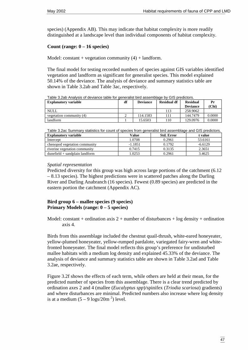
May 2002 Habitat requirements of fauna of CPP and LMD
47
species) (Appendix AB). This may indicate that habitat complexity is more readilydistinguished at a landscape level than individual components of habitat complexity.
Count (range: 0 – 16 species)
Model: constant + vegetation community (4) + landform.
The final model for testing recorded numbers of species against GIS variables identifiedvegetation and landform as significant for generalist species. This model explained50.14% of the deviance. The analysis of deviance and summary statistics table areshown in Table 3.2ab and Table 3ac, respectively.
Table 3.2ab Analysis of deviance table for generalist bird assemblage by GIS predictors.Explanatory variable df Deviance Residual df Residual
DeviancePr
(Chi)NULL 113 258.9062vegetation community (4) 2 114.1583 111 144.7479 0.0000landform 1 15.6503 110 129.0976 0.0000
Table 3.2ac Summary statistics for count of species from generalist bird assemblage and GIS predictors.Explanatory variable Value Std. Error t valueIntercept 1.0708 0.2961 53.6161chenopod vegetation community -1.1851 0.1792 -6.6129riverine vegetation community 0.7415 0.3135 2.3651dunefield + sandplain landform 1.0253 0.2961 3.4625
Spatial representationPredicted diversity for this group was high across large portions of the catchment (6.12– 8.13 species). The highest predictions were in scattered patches along the DarlingRiver and Darling Anabranch (16 species). Fewest (0.89 species) are predicted in theeastern portion the catchment (Appendix AC).
Bird group 6 – mallee species (9 species)Primary Models (range: 0 – 5 species)
Model: constant + ordination axis 2 + number of disturbances + log density + ordinationaxis 4.
Birds from this assemblage included the chestnut quail-thrush, white-eared honeyeater,yellow-plumed honeyeater, yellow-rumped pardalote, variegated fairy-wren and white-fronted honeyeater. The final model reflects this group’s preference for undisturbedmallee habitats with a medium log density and explained 45.33% of the deviance. Theanalysis of deviance and summary statistics table are shown in Table 3.2ad and Table3.2ae, respectively.
Figure 3.2f shows the effects of each term, while others are held at their mean, for thepredicted number of species from this assemblage. There is a clear trend predicted byordination axes 2 and 4 (mallee (Eucalyptus spp)/spinifex (Triodia scariosa) gradients)and where disturbances are minimal. Predicted numbers also increase where log densityis at a medium (5 – 9 logs/20m 2) level.
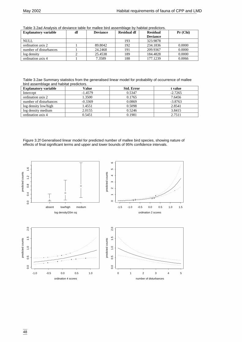
May 2002 Habitat requirements of fauna of CPP and LMD
48
Table 3.2ad Analysis of deviance table for mallee bird assemblage by habitat predictors.Explanatory variable df Deviance Residual df Residual
DeviancePr (Chi)
NULL 193 323.9878ordination axis 2 1 89.8042 192 234.1836 0.0000number of disturbances 1 24.2468 191 209.9367 0.0000log density 2 25.4538 189 184.4828 0.0000ordination axis 4 1 7.3589 188 177.1239 0.0066
Table 3.2ae Summary statistics from the generalised linear model for probability of occurrence of malleebird assemblage and habitat predictors.Explanatory variable Value Std. Error t valueIntercept -1.4579 0.5347 -2.7265ordination axis 2 1.3500 0.1765 7.6456number of disturbances -0.3369 0.0869 -3.8763log density low/high 1.4551 0.5098 2.8541log density medium 2.0155 0.5246 3.8415ordination axis 4 0.5451 0.1981 2.7511
Figure 3.2f Generalised linear model for predicted number of mallee bird species, showing nature ofeffects of final significant terms and upper and lower bounds of 95% confidence intervals.
log density/20m sq
pred
icte
d co
unts
0.0
0.4
0.8
1.2
1.6
absent low/high medium
ordination 2 scores
pred
icte
d co
unts
-1.5 -1.0 -0.5 0.0 0.5 1.0 1.5
01
23
45
6
ordination 4 scores
pred
icte
d co
unts
-1.0 -0.5 0.0 0.5 1.0
0.0
0.5
1.0
1.5
2.0
number of disturbances
pred
icte
d co
unts
0 1 2 3 4 5
0.0
0.5
1.0
1.5
2.0

May 2002 Habitat requirements of fauna of CPP and LMD
49
Secondary ModelsHabitat suitability (range: 0.04 – 4.55 species)
Model: constant + vegetation community (4).
Vegetation community was the only variable significant for predicting diversity ofmallee species. Mallee (Eucalyptus spp) communities are the most likely habitat withchenopod (Maireana spp) shrublands the least favourable for this group of birds. Themodel explained 65.26% of the deviance and the analysis of deviance and summarystatistics are shown in Table 3.2af and Table 3.2ag, respectively.
Table 3.2af Analysis of deviance table for mallee bird assemblage by GIS predictors.Explanatory variable df Deviance Residual
dfResidualDeviance
Pr (Chi)
NULL 113 97.7528vegetation community (4) 2 63.7991 111 33.9537 0.0000
Table 3.2ag Summary statistics for predicted abundance of species from mallee bird assemblage and GISpredictors.Explanatory variable Value Std. Error t valueIntercept -0.6734 0.1871 -3.5990chenopod -1.2890 0.6247 -2.0632mallee 1.3220 0.2208 5.9868
Spatial representationGreatest diversity for this assemblage was predicted for mallee (Eucalyptus spp)communities. However, it was not a high number (1.91 species) given the number ofpotential species. Lowest diversity was predicted to occur in chenopod (Maireana spp)shrublands (0.14 species) with belah (Casuarina pauper) woodlands and riverinecommunities equally diverse (0.50 species) (Appendix AD).
Count (range: 0 – 5 species)
Model: constant + vegetation community (4) + mean annual rainfall.
Vegetation and rainfall were identified as significant GIS terms for the count data. Themodel explained 51.86% of the deviance and the analysis of deviance and summarystatistics are shown in Table 3.2ah and Table 3.2ai, respectively. Mallee (Eucalyptusspp) communities and mean annual rainfall were predictors of greater assemblagediversity and, by implication, favourable habitat attributes.
Table 3.2ah Analysis of deviance table for mallee bird assemblage by GIS predictors.Explanatory variable df Deviance Residual df Residual
DeviancePr (Chi)
NULL 113 203.3352vegetation community (4) 2 92.9056 111 110.4296 0.0000mean annual rainfall 1 12.5487 110 97.8809 0.0003
Table 3.2ai Summary statistics for count of species from mallee bird assemblage and GIS predictors.Explanatory variable Value Std. Error t valueIntercept -5.1621 1.2262 -4.2096chenopod vegetation community -1.9875 1.0087 -1.9703mallee vegetation community 1.6825 0.2450 6.8664mean annual rainfall 0.0161 0.0045 3.5111
May 2002 Habitat requirements of fauna of CPP and LMD
50
Spatial representationThe spatial interpolation of the model illustrates a clear north-west to south-eastgradient. Greater diversity is predicted in mallee (Eucalyptus spp) communities, whichgradually decreases north-westward across the catchment according to the rainfallgradient. This results in higher numbers in the south-east, excluding the Murray Rivercorridor, where rainfall is higher (4.3 species maximum) and fewer species (0.02species) in the drier north-west (Appendix AE).
Summary of primary modelsAppendix AF summarises the effects of the variables on the diversity of each speciesgroup. The most frequently identified variables for the bird group models were distancefrom water (natural or artificial), cover of woodland and number of disturbances. Thenumber of disturbances had a consistently negative impact upon the predicted diversityof bird species while woodland was consistently positive. Distance from water also hada positive effect, except for the riverine species group where this was expected.
Vegetation ordinations axes 2 and 3, density of logs and cryptogam cover were the nextmost frequently identified variables. The diversity of woodland and riparian speciesdecreased in both belah/rosewood communities (ordination axis 3) and malleecommunities (ordination axis 2). The diversity of mallee bird species was increased inmallee/spinifex communities and the diversity of generalists bird species was greater inbelah/rosewood communities. Cryptogam cover and density of logs both had a positiveeffect on species diversity. It is unclear why cryptogam cover would have an effect,however it may be an indicator of fewer disturbances, i.e. less grazing pressure, orgreater rainfall.
Tall shrubland had a positive effect for both the riparian assemblage and the generalistassemblage. Low shrubland was significant for both the riparian assemblage and thewoodland and riparian assemblage, exhibiting a negative effect on the diversity of bothgroups. Hummock grass (spinifex) was included in low shrubland and it is reasonablefor a negative effect to be evident for both species groups. Spinifex favours sandy soilsand is associated with mallee communities, previously identified as having a reducedeffect on the diversity of woodland and riparian bird species.
The least frequently identified determinants of diversity were ordination axis 1 (a weakindicator of increasing mallee/spinifex cover), ordination axis 4 (increasingmallee/white cypress pine cover), habitat complexity and ground cover. All variableshad a positive effect on species diversity, except ordination axis 1 which had a negativeeffect.
REPTILES
3.2.3 Classification and ordinationA total of 48 species were detected from the nocturnal and diurnal searches across 186sites (8 sites recorded no species). Species that occurred only once were excluded andpresence/absence data was analysed.
Site classificationThe classification of the sites revealed six groups (ANOSIM, pseudo F=1.40, p<0.001)(Appendix AH) with the first split separating mallee (Eucalyptus spp) sites (Group VI,27 sites) from the remainder. The next split separated the bluebush (Maireana spp)
May 2002 Habitat requirements of fauna of CPP and LMD
51
shrubland sites (Group V, 10 sites). The next group of sites to be defined was thosewhich recorded few species (Group IV, five sites). At a lower level of fusion, Group II(56 sites) and Group III (31 sites) emerged and were spread equally across the studyregion. Group I (57 sites) was revealed at the lowest fusion level and was composedmostly of sites in the west of the study region.
Species classificationFive species groups were revealed from the classification (ANOSIM, pseudo F=1.53,p<0.001) (Appendix AI), split primarily according to preference for mallee (Eucalyptusspp) habitat (Group 5, seven species). The remaining groups were generalist species andhabitat specialists. Group 4 (one species) was a bluebush (Maireana spp) shrublandhabitat species, Group 3 (20 species) was composed of generalist habitat species andGroup 2 (five species) was a group of generalists and bluebush (Maireana spp) habitatspecies. Group 1 (seven species) was composed of generalist and mallee (Eucalyptusspp) shrubland habitat species.
EvaluationThe final stage of the classification process was construction of a two-way tableillustrating the distribution of species across sites (Appendix AJ). Site groups weretested against floristic data to determine the associated vegetation communities to helpwith naming the reptile species groups. Table 3.3a summarises these results.
OrdinationThe results from the principal axis correlation did not reveal any species highlycorrelated to vegetation gradients (r<0.4, p > 0.05). Bubble plots of the abundance ofeach species group against each ordination axis revealed a trend for the abundance ofGroup 3 (generalists species) to increase along ordination axis 3 towards belah(Casuarina pauper) and rosewood (Alectryon oleifolius). An increasing trend inabundance of Group 1 (generalist and mallee (Eucalyptus spp) reptile species) andGroup 5 (mallee (Eucalyptus spp) reptile specialists) was noted along ordination axis 2towards mallee (Eucalyptus spp)/spinifex (Triodia scariosa) communities.
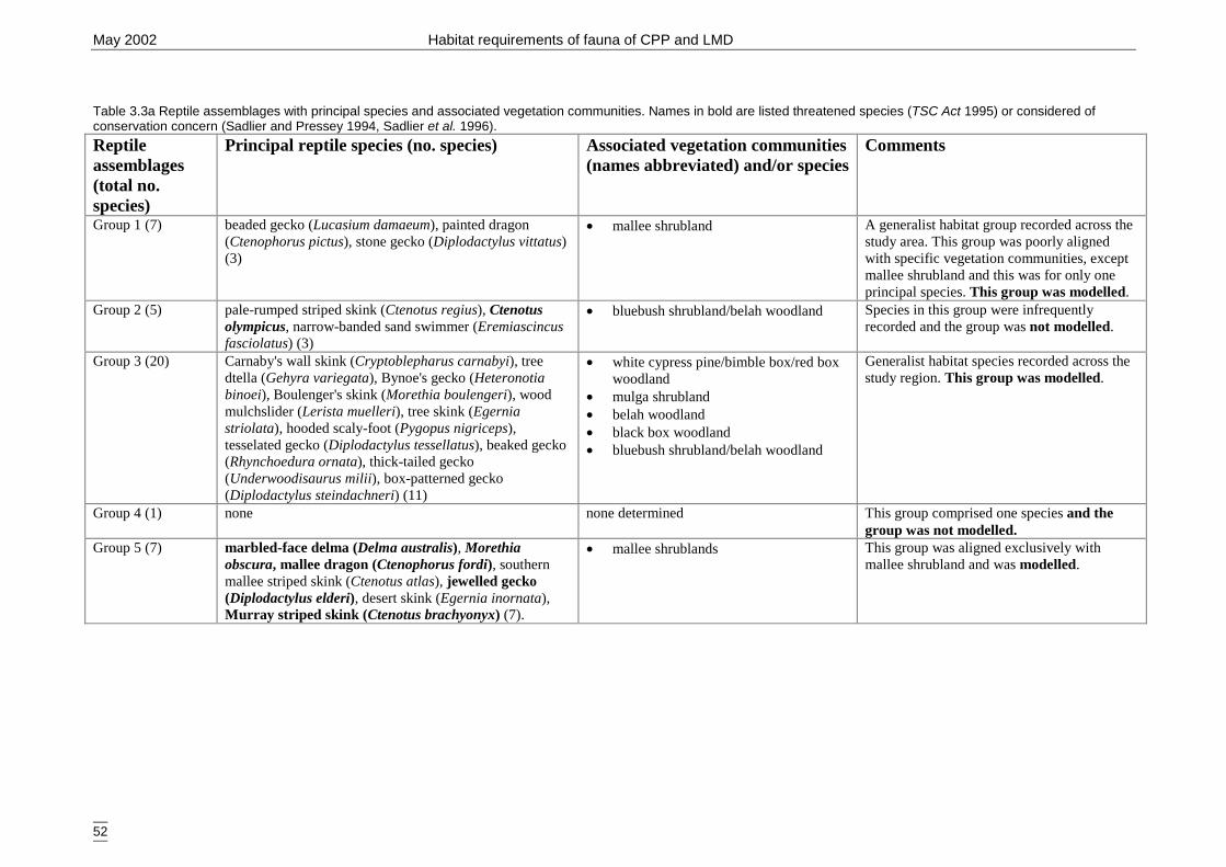
May 2002 Habitat requirements of fauna of CPP and LMD
52
Table 3.3a Reptile assemblages with principal species and associated vegetation communities. Names in bold are listed threatened species (TSC Act 1995) or considered ofconservation concern (Sadlier and Pressey 1994, Sadlier et al. 1996).Reptileassemblages(total no.species)
Principal reptile species (no. species) Associated vegetation communities(names abbreviated) and/or species
Comments
Group 1 (7) beaded gecko (Lucasium damaeum), painted dragon(Ctenophorus pictus), stone gecko (Diplodactylus vittatus)(3)
� mallee shrubland A generalist habitat group recorded across thestudy area. This group was poorly alignedwith specific vegetation communities, exceptmallee shrubland and this was for only oneprincipal species. This group was modelled.
Group 2 (5) pale-rumped striped skink (Ctenotus regius), Ctenotusolympicus, narrow-banded sand swimmer (Eremiascincusfasciolatus) (3)
� bluebush shrubland/belah woodland Species in this group were infrequentlyrecorded and the group was not modelled.
Group 3 (20) Carnaby's wall skink (Cryptoblepharus carnabyi), treedtella (Gehyra variegata), Bynoe's gecko (Heteronotiabinoei), Boulenger's skink (Morethia boulengeri), woodmulchslider (Lerista muelleri), tree skink (Egerniastriolata), hooded scaly-foot (Pygopus nigriceps),tesselated gecko (Diplodactylus tessellatus), beaked gecko(Rhynchoedura ornata), thick-tailed gecko(Underwoodisaurus milii), box-patterned gecko(Diplodactylus steindachneri) (11)
� white cypress pine/bimble box/red boxwoodland
� mulga shrubland� belah woodland� black box woodland� bluebush shrubland/belah woodland
Generalist habitat species recorded across thestudy region. This group was modelled.
Group 4 (1) none none determined This group comprised one species and thegroup was not modelled.
Group 5 (7) marbled-face delma (Delma australis), Morethiaobscura, mallee dragon (Ctenophorus fordi), southernmallee striped skink (Ctenotus atlas), jewelled gecko(Diplodactylus elderi), desert skink (Egernia inornata),Murray striped skink (Ctenotus brachyonyx) (7).
� mallee shrublands This group was aligned exclusively withmallee shrubland and was modelled.
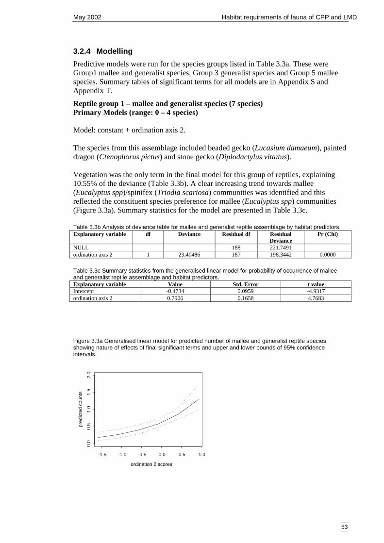
May 2002 Habitat requirements of fauna of CPP and LMD
53
3.2.4 ModellingPredictive models were run for the species groups listed in Table 3.3a. These wereGroup1 mallee and generalist species, Group 3 generalist species and Group 5 malleespecies. Summary tables of significant terms for all models are in Appendix S andAppendix T.
Reptile group 1 – mallee and generalist species (7 species)Primary Models (range: 0 – 4 species)
Model: constant + ordination axis 2.
The species from this assemblage included beaded gecko (Lucasium damaeum), painteddragon (Ctenophorus pictus) and stone gecko (Diplodactylus vittatus).
Vegetation was the only term in the final model for this group of reptiles, explaining10.55% of the deviance (Table 3.3b). A clear increasing trend towards mallee(Eucalyptus spp)/spinifex (Triodia scariosa) communities was identified and thisreflected the constituent species preference for mallee (Eucalyptus spp) communities(Figure 3.3a). Summary statistics for the model are presented in Table 3.3c.
Table 3.3b Analysis of deviance table for mallee and generalist reptile assemblage by habitat predictors.Explanatory variable df Deviance Residual df Residual
DeviancePr (Chi)
NULL 188 221.7491ordination axis 2 1 23.40486 187 198.3442 0.0000
Table 3.3c Summary statistics from the generalised linear model for probability of occurrence of malleeand generalist reptile assemblage and habitat predictors.Explanatory variable Value Std. Error t valueIntercept -0.4734 0.0959 -4.9317ordination axis 2 0.7906 0.1658 4.7683
Figure 3.3a Generalised linear model for predicted number of mallee and generalist reptile species,showing nature of effects of final significant terms and upper and lower bounds of 95% confidenceintervals.
ordination 2 scores
pred
icte
d co
unts
-1.5 -1.0 -0.5 0.0 0.5 1.0
0.0
0.5
1.0
1.5
2.0
May 2002 Habitat requirements of fauna of CPP and LMD
54
Secondary ModelsHabitat suitability (range: 0.42 –1.68 species)
No landscape-scale terms were significant for predicting preferred habitat for thisassemblage.
Count (range: 0 – 4 species)
Model: constant + vegetation community (4) + mean annual rainfall.
At a landscape level, the model testing GIS variables against the recorded number ofspecies in the assemblage identified vegetation and mean annual rainfall as the mostsignificant terms, explaining 22.40% of the deviance (Table 3.3d). Summary statisticsare shown in Table 3.3e and indicate that mallee (Eucalyptus spp) communities and lowrainfall were the best predictors.
Table 3.3d Analysis of deviance table for of mallee and generalist reptile assemblage by GIS predictors.Explanatory variable df Deviance Residual df Residual
DeviancePr
(Chi)NULL 113 141.2970vegetation community (4) 2 26.3196 111 114.9774 0.0000mean annual rainfall 1 5.3321 110 109.6453 0.0209
Table 3.3e Summary statistics for count of species from of mallee and generalist reptile assemblage andGIS predictors.Explanatory variable Value Std. Error t valueIntercept 2.4910 1.1306 2.2032chenopod + riverine vegetation community -0.7331 0.3118 -2.3509mallee vegetation community 0.6450 0.2121 3.0405mean annual rainfall -0.0108 0.0044 -2.4324
Spatial representationThe spatial interpolation of the model reveals that the maximum number of species(more than 2.0 species) are predicted to occur in the upper western portions of thecatchment, corresponding to mallee (Eucalyptus spp)/spinifex (Triodia scariosa)communities in regions of lower rainfall (Appendix AK).
Reptile group 3 – generalist species (20 species)Primary Models (range: 0 – 8 species)
Model: constant + ordination axis 2 + ordination axis 3 + log density + low shrub cover+ woodland cover.
This was the largest reptile group and included Carnaby's wall skink (Cryptoblepharuscarnabyi), tree dtella (Gehyra variegata), Bynoe's gecko (Heteronotia binoei),Boulenger's skink (Morethia boulengeri), wood mulchslider (Lerista muelleri), treeskink (Egernia striolata), hooded scaly-foot (Pygopus nigriceps), tesselated gecko(Diplodactylus tessellatus), beaked gecko (Rhynchoedura ornata), thick-tailed gecko(Underwoodisaurus milii) and box-patterned gecko (Diplodactylus steindachneri).
The model explained 46.73% of the deviance (Table 3.3f) and describes the vegetationtypes and microhabitat variables that predict these species’ occurrence. Summary

May 2002 Habitat requirements of fauna of CPP and LMD
55
statistics are shown in Table 3.3g. Figure 3.3b shows the nature of the effects of eachterm on predicted numbers, with the other terms held at their mean.
There is a clear trend away from mallee (Eucalyptus spp)/spinifex (Triodia scariosa)communities on ordination axis 2 with greatest numbers predicted for pine (Callitrisglaucophylla) and wilga (Geijera parviflora) associations. Ordination axis 3 also showsthe trend towards belah (Casuarina pauper) and pine (Callitris glaucophylla)communities in addition to a weaker trend for mallee (Eucalyptus spp) communities.Structural indicators are sparse woodland (<10% cover) and sparse low shrub cover(<10%). A high density of logs (>10/20m2) is also a good predictor of generalist reptilespecies diversity.
Table 3.3f Analysis of deviance table for generalist reptile assemblage by habitat predictors.Explanatoryvariable
df Deviance Residual df ResidualDeviance
Pr (Chi)
NULL 188 312.7277ordination axis 2 1 103.1667 187 209.5610 0.0000ordination axis 3 1 16.6731 186 192.8879 0.0000log density 2 14.7897 184 178.0982 0.0006low shrub cover 1 6.3695 183 171.7287 0.0116woodland cover 1 5.1648 182 166.5638 0.0230
Table 3.3g Summary statistics from the generalised linear model for probability of occurrence of generalistreptile assemblage and habitat predictors.Explanatory variable Value Std. Error t valueIntercept 0.6601 0.1476 4.4703ordination axis 2 -6.6944 1.0196 -6.5656ordination axis 3 1.5492 0.5005 3.0948log density low/medium (0 – 9) 0.3393 0.1531 2.2158log density high (10+) 0.5042 0.1600 3.1514low shrub >10% cover -0.2779 0.1052 -2.6413woodland <10% cover 0.2155 0.0940 2.2927
Figure 3.3b Generalised linear model for predicted number of generalist reptile species, showing nature ofeffects of final significant terms and upper and lower bounds of 95% confidence intervals.
ordination 2 scores
pred
icte
d co
unts
-1.5 -1.0 -0.5 0.0 0.5 1.0
01
23
45
ordination 3 scores
pred
icte
d co
unts
-1.0 -0.5 0.0 0.5 1.0
01
23
45
6
log density/20m sq
pred
icte
d co
unts
24
68
absent low/medium high
low shrub cover
pred
icte
d co
unts
12
34
56
<10% >10%
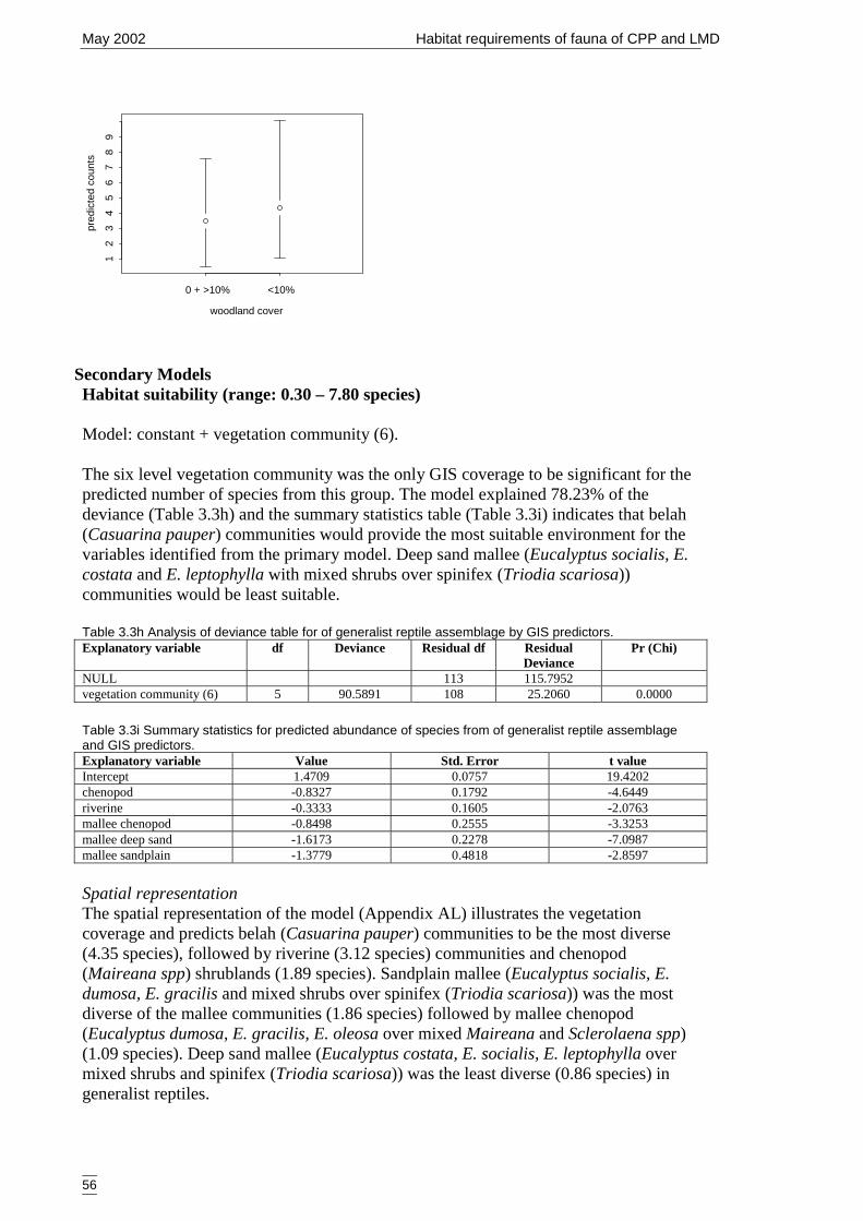
May 2002 Habitat requirements of fauna of CPP and LMD
56
Secondary ModelsHabitat suitability (range: 0.30 – 7.80 species)
Model: constant + vegetation community (6).
The six level vegetation community was the only GIS coverage to be significant for thepredicted number of species from this group. The model explained 78.23% of thedeviance (Table 3.3h) and the summary statistics table (Table 3.3i) indicates that belah(Casuarina pauper) communities would provide the most suitable environment for thevariables identified from the primary model. Deep sand mallee (Eucalyptus socialis, E.costata and E. leptophylla with mixed shrubs over spinifex (Triodia scariosa))communities would be least suitable.
Table 3.3h Analysis of deviance table for of generalist reptile assemblage by GIS predictors.Explanatory variable df Deviance Residual df Residual
DeviancePr (Chi)
NULL 113 115.7952vegetation community (6) 5 90.5891 108 25.2060 0.0000
Table 3.3i Summary statistics for predicted abundance of species from of generalist reptile assemblageand GIS predictors.Explanatory variable Value Std. Error t valueIntercept 1.4709 0.0757 19.4202chenopod -0.8327 0.1792 -4.6449riverine -0.3333 0.1605 -2.0763mallee chenopod -0.8498 0.2555 -3.3253mallee deep sand -1.6173 0.2278 -7.0987mallee sandplain -1.3779 0.4818 -2.8597
Spatial representationThe spatial representation of the model (Appendix AL) illustrates the vegetationcoverage and predicts belah (Casuarina pauper) communities to be the most diverse(4.35 species), followed by riverine (3.12 species) communities and chenopod(Maireana spp) shrublands (1.89 species). Sandplain mallee (Eucalyptus socialis, E.dumosa, E. gracilis and mixed shrubs over spinifex (Triodia scariosa)) was the mostdiverse of the mallee communities (1.86 species) followed by mallee chenopod(Eucalyptus dumosa, E. gracilis, E. oleosa over mixed Maireana and Sclerolaena spp)(1.09 species). Deep sand mallee (Eucalyptus costata, E. socialis, E. leptophylla overmixed shrubs and spinifex (Triodia scariosa)) was the least diverse (0.86 species) ingeneralist reptiles.
woodland cover
pred
icte
d co
unts
12
34
56
78
9
0 + >10% <10%
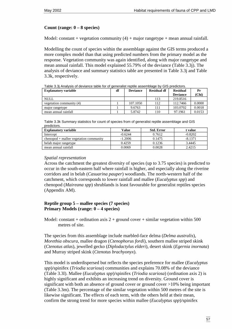
May 2002 Habitat requirements of fauna of CPP and LMD
57
Count (range: 0 – 8 species)
Model: constant + vegetation community (4) + major rangetype + mean annual rainfall.
Modelling the count of species within the assemblage against the GIS terms produced amore complex model than that using predicted numbers from the primary model as theresponse. Vegetation community was again identified, along with major rangetype andmean annual rainfall. This model explained 55.79% of the deviance (Table 3.3j). Theanalysis of deviance and summary statistics table are presented in Table 3.3j and Table3.3k, respectively.
Table 3.3j Analysis of deviance table for of generalist reptile assemblage by GIS predictors.Explanatory variable df Deviance Residual df Residual
DeviancePr
(Chi)NULL 113 219.8516vegetation community (4) 1 107.1050 112 112.7466 0.0000major rangetype 1 9.6763 111 103.0702 0.0018mean annual rainfall 1 5.8742 110 97.1961 0.0153
Table 3.3k Summary statistics for count of species from of generalist reptile assemblage and GISpredictors.Explanatory variable Value Std. Error t valueIntercept -0.6244 0.7612 -0.8202chenopod + mallee vegetation community -1.2006 0.1475 -8.1371belah major rangetype 0.4259 0.1236 3.4445mean annual rainfall 0.0069 0.0028 2.4215
Spatial representationAcross the catchment the greatest diversity of species (up to 3.75 species) is predicted tooccur in the south-eastern half where rainfall is higher, and especially along the riverinecorridors and in belah (Casuarina pauper) woodlands. The north-western half of thecatchment, which corresponds to lower rainfall and mallee (Eucalyptus spp) andchenopod (Maireana spp) shrublands is least favourable for generalist reptiles species(Appendix AM).
Reptile group 5 – mallee species (7 species)Primary Models (range: 0 – 4 species)
Model: constant + ordination axis 2 + ground cover + similar vegetation within 500metres of site.
The species from this assemblage include marbled-face delma (Delma australis),Morethia obscura, mallee dragon (Ctenophorus fordi), southern mallee striped skink(Ctenotus atlas), jewelled gecko (Diplodactylus elderi), desert skink (Egernia inornata)and Murray striped skink (Ctenotus brachyonyx).
This model is underdispersed but reflects the species preference for mallee (Eucalyptusspp)/spinifex (Triodia scariosa) communities and explains 70.08% of the deviance(Table 3.3l). Mallee (Eucalyptus spp)/spinifex (Triodia scariosa) (ordination axis 2) ishighly significant and exhibits an increasing trend on diversity. Ground cover issignificant with both an absence of ground cover or ground cover >10% being important(Table 3.3m). The percentage of the similar vegetation within 500 metres of the site islikewise significant. The effects of each term, with the others held at their mean,confirm the strong trend for more species within mallee (Eucalyptus spp)/spinifex
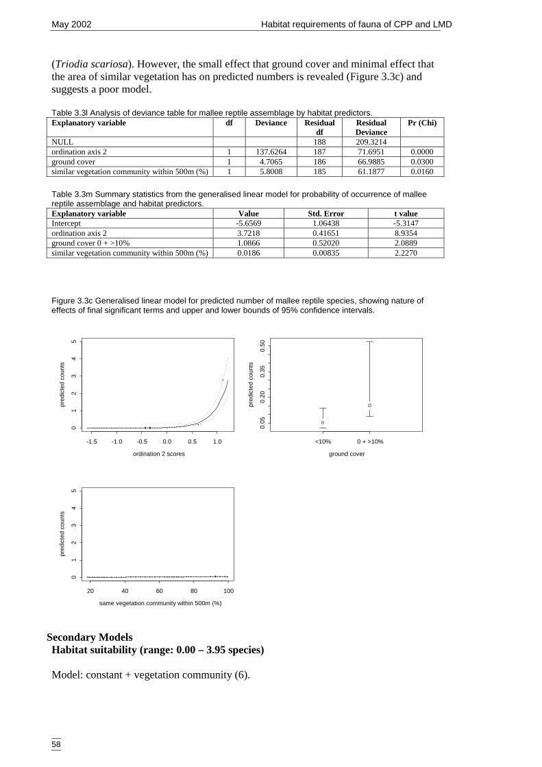
May 2002 Habitat requirements of fauna of CPP and LMD
58
(Triodia scariosa). However, the small effect that ground cover and minimal effect thatthe area of similar vegetation has on predicted numbers is revealed (Figure 3.3c) andsuggests a poor model.
Table 3.3l Analysis of deviance table for mallee reptile assemblage by habitat predictors.Explanatory variable df Deviance Residual
dfResidualDeviance
Pr (Chi)
NULL 188 209.3214ordination axis 2 1 137.6264 187 71.6951 0.0000ground cover 1 4.7065 186 66.9885 0.0300similar vegetation community within 500m (%) 1 5.8008 185 61.1877 0.0160
Table 3.3m Summary statistics from the generalised linear model for probability of occurrence of malleereptile assemblage and habitat predictors.Explanatory variable Value Std. Error t valueIntercept -5.6569 1.06438 -5.3147ordination axis 2 3.7218 0.41651 8.9354ground cover 0 + >10% 1.0866 0.52020 2.0889similar vegetation community within 500m (%) 0.0186 0.00835 2.2270
Figure 3.3c Generalised linear model for predicted number of mallee reptile species, showing nature ofeffects of final significant terms and upper and lower bounds of 95% confidence intervals.
Secondary ModelsHabitat suitability (range: 0.00 – 3.95 species)
Model: constant + vegetation community (6).
ordination 2 scores
pred
icte
d co
unts
-1.5 -1.0 -0.5 0.0 0.5 1.0
01
23
45
ground cover
pred
icte
d co
unts
0.05
0.20
0.35
0.50
<10% 0 + >10%
same vegetation community within 500m (%)
pred
icte
d co
unts
20 40 60 80 100
01
23
45
May 2002 Habitat requirements of fauna of CPP and LMD
59
The six level vegetation community was the only term in the final model that wassignificant for the predicted diversity of this group. The model explained 77.29% of thedeviance (Table 3.3n). The summary statistics table (Table 3.3o) indicates that deepsand mallee (Eucalyptus socialis, E. costata and E. leptophylla with mixed shrubs overspinifex (Triodia scariosa)) followed by sandplain mallee (Eucalyptus socialis, E.dumosa and E. gracilis with mixed shrubs over spinifex (Triodia scariosa))communities provide the most suitable environment for this species group.
Table 3.3n Analysis of deviance table for mallee reptile assemblage by GIS predictors.Explanatory variable df Deviance Residual df Residual
DeviancePr (Chi)
NULL 113 113.9180vegetation community (6) 3 88.0558 110 25.8622 0.0000
Table 3.3o Summary statistics for predicted abundance of species from mallee reptile assemblage andGIS predictors.Explanatory variable Value Std. Error t valueIntercept -2.8385 0.4742 -5.9857mallee chenopod 1.7573 0.7424 2.3670mallee deep sand 3.3128 0.4997 6.6284mallee sandplain 2.8427 0.6883 4.1297
Spatial representationThe spatial interpolation of the model illustrates the vegetation coverage and predictsgreater diversity to occur in the bands of mallee (Eucalyptus spp) communities that lienorth east/south west across the catchment (Appendix AN). In these areas more speciesare predicted in the deep sand mallee (Eucalyptus socialis, E. costata and E. leptophyllawith mixed shrubs over spinifex (Triodia scariosa)) (1.60 species) compared to thesandplain mallee (Eucalyptus socialis, E. dumosa and E. gracilis with mixed shrubsover spinifex (Triodia scariosa)) (1.00 species) and the mallee chenopod (Eucalyptusdumosa, E. gracilis, E. oleosa over mixed Maireana and Sclerolaena spp) areas (0.34species). The remainder of the catchment covered by belah (Casuarina pauper)woodlands, riverine communities and chenopod (Maireana spp) shrublands werepredicted to support negligible mallee reptile species diversity (0.06 species).
Count (range: 0 – 4 species)
Model: constant + landform.
Landform, specifically dunefields, was the only landscape variable significant for therecorded number of species of this assemblage. This model explained 34.28% of thedeviance (Table 3.3p) and the summary statistics are presented in Table 3.3q.
Table 3.3p Analysis of deviance table for mallee reptile assemblage by GIS predictors.Explanatory variable df Deviance Residual df Residual
DeviancePr
(Chi)NULL 113 153.8206landform 1 52.7378 112 101.0828 0.0000
Table 3.3q Summary statistics for count of species from mallee reptile assemblage and GIS predictors.Explanatory variable Value Std. Error t valueIntercept 0.0000 0.1490 0.0000sandplain + alluvial landform -2.4423 0.4344 -5.6219
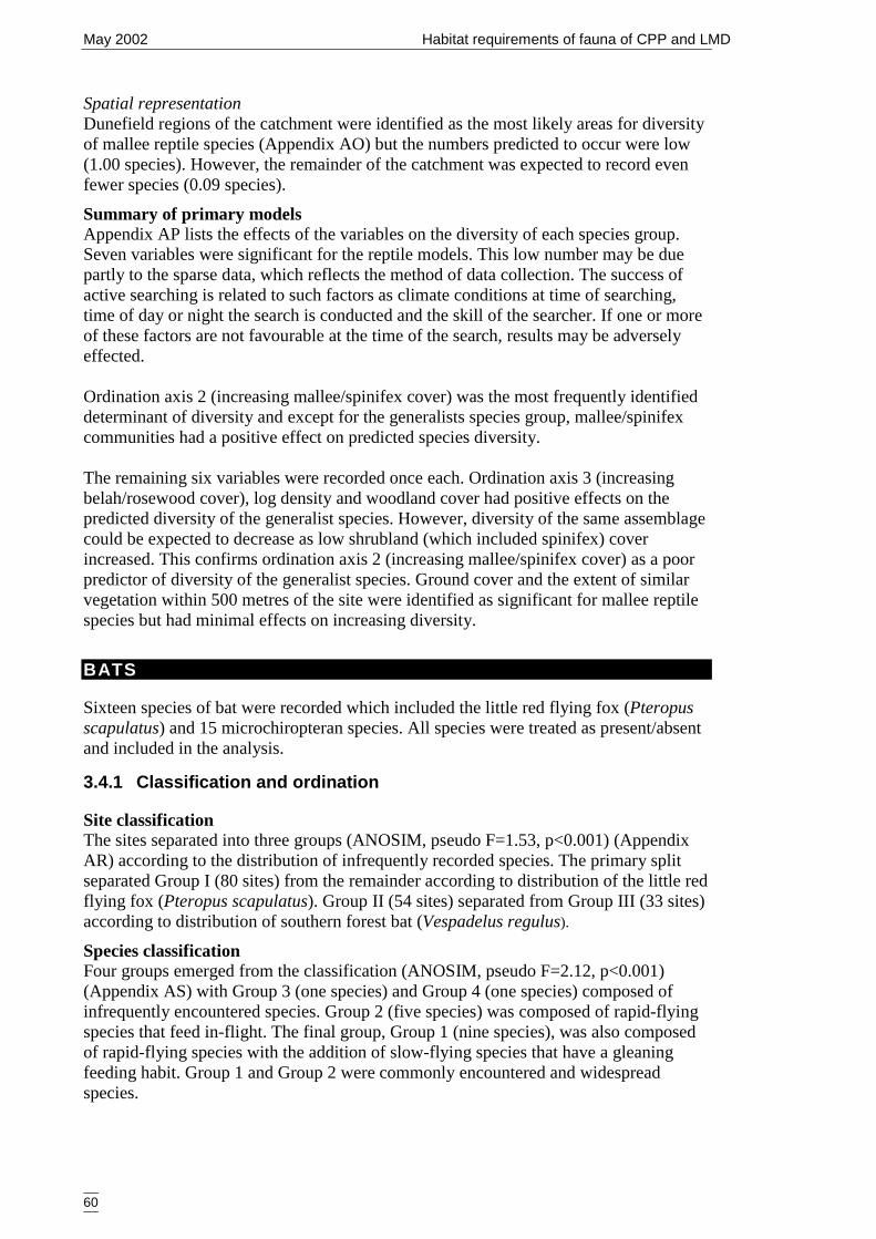
May 2002 Habitat requirements of fauna of CPP and LMD
60
Spatial representationDunefield regions of the catchment were identified as the most likely areas for diversityof mallee reptile species (Appendix AO) but the numbers predicted to occur were low(1.00 species). However, the remainder of the catchment was expected to record evenfewer species (0.09 species).
Summary of primary modelsAppendix AP lists the effects of the variables on the diversity of each species group.Seven variables were significant for the reptile models. This low number may be duepartly to the sparse data, which reflects the method of data collection. The success ofactive searching is related to such factors as climate conditions at time of searching,time of day or night the search is conducted and the skill of the searcher. If one or moreof these factors are not favourable at the time of the search, results may be adverselyeffected.
Ordination axis 2 (increasing mallee/spinifex cover) was the most frequently identifieddeterminant of diversity and except for the generalists species group, mallee/spinifexcommunities had a positive effect on predicted species diversity.
The remaining six variables were recorded once each. Ordination axis 3 (increasingbelah/rosewood cover), log density and woodland cover had positive effects on thepredicted diversity of the generalist species. However, diversity of the same assemblagecould be expected to decrease as low shrubland (which included spinifex) coverincreased. This confirms ordination axis 2 (increasing mallee/spinifex cover) as a poorpredictor of diversity of the generalist species. Ground cover and the extent of similarvegetation within 500 metres of the site were identified as significant for mallee reptilespecies but had minimal effects on increasing diversity.
BATS
Sixteen species of bat were recorded which included the little red flying fox (Pteropusscapulatus) and 15 microchiropteran species. All species were treated as present/absentand included in the analysis.
3.4.1 Classification and ordination
Site classificationThe sites separated into three groups (ANOSIM, pseudo F=1.53, p<0.001) (AppendixAR) according to the distribution of infrequently recorded species. The primary splitseparated Group I (80 sites) from the remainder according to distribution of the little redflying fox (Pteropus scapulatus). Group II (54 sites) separated from Group III (33 sites)according to distribution of southern forest bat (Vespadelus regulus).
Species classificationFour groups emerged from the classification (ANOSIM, pseudo F=2.12, p<0.001)(Appendix AS) with Group 3 (one species) and Group 4 (one species) composed ofinfrequently encountered species. Group 2 (five species) was composed of rapid-flyingspecies that feed in-flight. The final group, Group 1 (nine species), was also composedof rapid-flying species with the addition of slow-flying species that have a gleaningfeeding habit. Group 1 and Group 2 were commonly encountered and widespreadspecies.
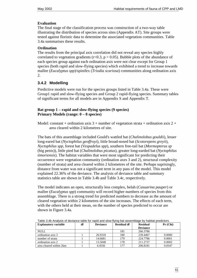
May 2002 Habitat requirements of fauna of CPP and LMD
61
EvaluationThe final stage of the classification process was construction of a two-way tableillustrating the distribution of species across sites (Appendix AT). Site groups weretested against floristic data to determine the associated vegetation communities. Table3.4a summarises these results.
OrdinationThe results from the principal axis correlation did not reveal any species highlycorrelated to vegetation gradients (r<0.3, p > 0.05). Bubble plots of the abundance ofeach species group against each ordination axis were not clear except for Group 1species (both rapid and slow-flying species) which exhibited a trend to increase towardsmallee (Eucalyptus spp)/spinifex (Triodia scariosa) communities along ordination axis2.
3.4.2 ModellingPredictive models were run for the species groups listed in Table 3.4a. These wereGroup1 rapid and slow-flying species and Group 2 rapid-flying species. Summary tablesof significant terms for all models are in Appendix S and Appendix T.
Bat group 1 – rapid and slow-flying species (9 species)Primary Models (range: 0 – 8 species)
Model: constant + ordination axis 3 + number of vegetation strata + ordination axis 2 +area cleared within 2 kilometres of site.
The bats of this assemblage included Gould's wattled bat (Chalinolobus gouldii), lesserlong-eared bat (Nyctophilus geoffroyi), little broad-nosed bat (Scotorepens greyii),Nyctophilus spp, forest bat (Vespadelus spp), southern free-tail bat (Mormopterus sp(big penis)), little pied bat (Chalinolobus picatus), greater long-earded bat (Nyctophilustimoriensis). The habitat variables that were most significant for predicting theiroccurrence were vegetation community (ordination axes 3 and 2), structural complexity(number of strata) and area cleared within 2 kilometres of the site. Perhaps suprisingly,distance from water was not a significant term in any pass of the model. This modelexplained 22.36% of the deviance. The analysis of deviance table and summarystatistics table are shown in Table 3.4b and Table 3.4c, respectively.
The model indicates an open, structurally less complex, belah (Casuarina pauper) ormallee (Eucalyptus spp) community will record higher numbers of species from thisassemblage. There is a strong trend for predicted numbers to decrease as the amount ofcleared vegetation within 2 kilometres of the site increases. The effects of each term,with the others held at their mean, on the number of species predicted to occur areshown in Figure 3.4a.
Table 3.4b Analysis of deviance table for rapid and slow-flying bat assemblage by habitat predictors.Explanatory variable df Deviance Residual df Residual
DeviancePr (Chi)
NULL 181 266.3786ordination axis 3 1 26.9318 180 239.4467 0.0000number of strata 1 14.6681 179 224.7786 0.0001ordination axis 2 1 13.5048 178 211.2737 0.0002area cleared within 2km 1 4.4556 177 206.8181 0.0347
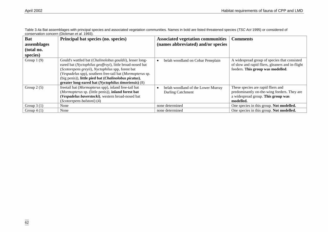
April 2002 Habitat requirements of fauna of CPP and LMD
62
Table 3.4a Bat assemblages with principal species and associated vegetation communities. Names in bold are listed threatened species (TSC Act 1995) or considered ofconservation concern (Dickman et al. 1993).Batassemblages(total no.species)
Principal bat species (no. species) Associated vegetation communities(names abbreviated) and/or species
Comments
Group 1 (9) Gould's wattled bat (Chalinolobus gouldii), lesser long-eared bat (Nyctophilus geoffroyi), little broad-nosed bat(Scotorepens greyii), Nyctophilus spp, forest bat(Vespadelus spp), southern free-tail bat (Mormopterus sp.(big penis)), little pied bat (Chalinolobus picatus),greater long-eared bat (Nyctophilus timoriensis) (8)
� belah woodland on Cobar Peneplain A widespread group of species that consistedof slow and rapid fliers, gleaners and in-flightfeeders. This group was modelled.
Group 2 (5) freetail bat (Mormopterus spp), inland free-tail bat(Mormopterus sp. (little penis)), inland forest bat(Vespadelus baverstocki), western broad-nosed bat(Scotorepens balstoni) (4)
� belah woodland of the Lower MurrayDarling Catchment
These species are rapid fliers andpredominantly on-the-wing feeders. They area widespread group. This group wasmodelled.
Group 3 (1) None none determined One species in this group. Not modelled.Group 4 (1) None none determined One species in this group. Not modelled.
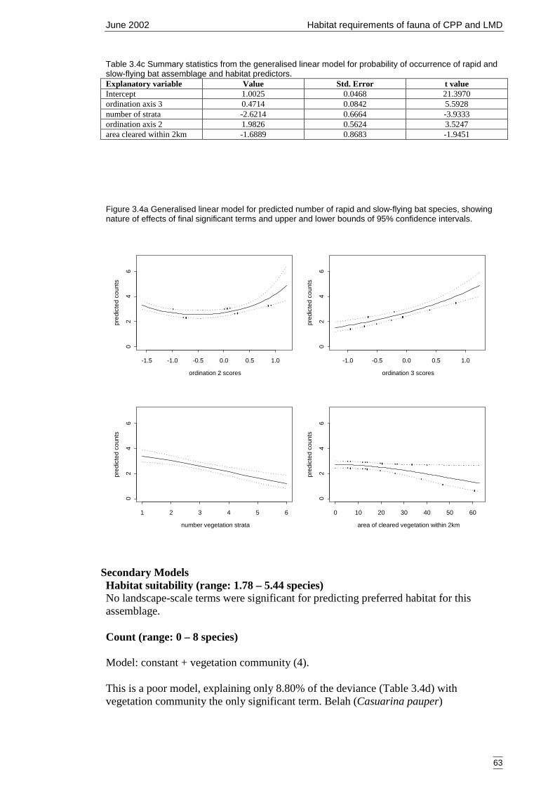
June 2002 Habitat requirements of fauna of CPP and LMD
63
Table 3.4c Summary statistics from the generalised linear model for probability of occurrence of rapid andslow-flying bat assemblage and habitat predictors.Explanatory variable Value Std. Error t valueIntercept 1.0025 0.0468 21.3970ordination axis 3 0.4714 0.0842 5.5928number of strata -2.6214 0.6664 -3.9333ordination axis 2 1.9826 0.5624 3.5247area cleared within 2km -1.6889 0.8683 -1.9451
Figure 3.4a Generalised linear model for predicted number of rapid and slow-flying bat species, showingnature of effects of final significant terms and upper and lower bounds of 95% confidence intervals.
Secondary ModelsHabitat suitability (range: 1.78 – 5.44 species)No landscape-scale terms were significant for predicting preferred habitat for thisassemblage.
Count (range: 0 – 8 species)
Model: constant + vegetation community (4).
This is a poor model, explaining only 8.80% of the deviance (Table 3.4d) withvegetation community the only significant term. Belah (Casuarina pauper)
ordination 2 scores
pred
icte
d co
unts
-1.5 -1.0 -0.5 0.0 0.5 1.0
02
46
ordination 3 scores
pred
icte
d co
unts
-1.0 -0.5 0.0 0.5 1.0
02
46
number vegetation strata
pred
icte
d co
unts
1 2 3 4 5 6
02
46
area of cleared vegetation within 2km
pred
icte
d co
unts
0 10 20 30 40 50 60
02
46
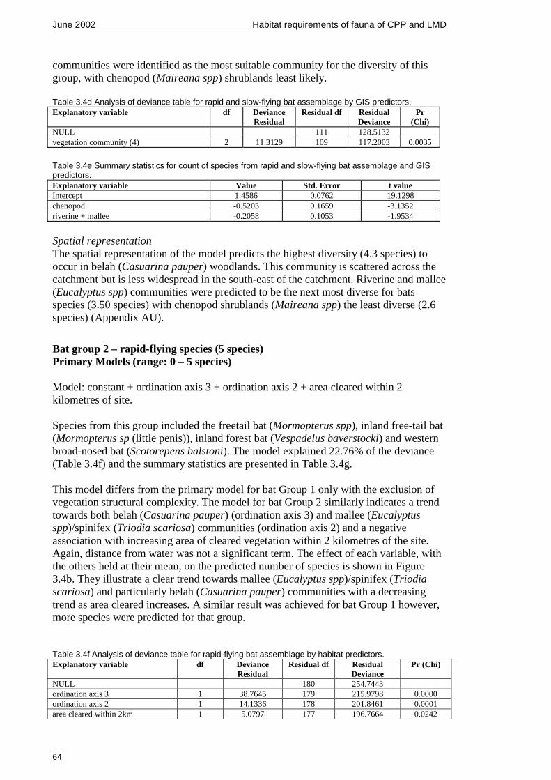
June 2002 Habitat requirements of fauna of CPP and LMD
64
communities were identified as the most suitable community for the diversity of thisgroup, with chenopod (Maireana spp) shrublands least likely.
Table 3.4d Analysis of deviance table for rapid and slow-flying bat assemblage by GIS predictors.Explanatory variable df Deviance
ResidualResidual df Residual
DeviancePr
(Chi)NULL 111 128.5132vegetation community (4) 2 11.3129 109 117.2003 0.0035
Table 3.4e Summary statistics for count of species from rapid and slow-flying bat assemblage and GISpredictors.Explanatory variable Value Std. Error t valueIntercept 1.4586 0.0762 19.1298chenopod -0.5203 0.1659 -3.1352riverine + mallee -0.2058 0.1053 -1.9534
Spatial representationThe spatial representation of the model predicts the highest diversity (4.3 species) tooccur in belah (Casuarina pauper) woodlands. This community is scattered across thecatchment but is less widespread in the south-east of the catchment. Riverine and mallee(Eucalyptus spp) communities were predicted to be the next most diverse for batsspecies (3.50 species) with chenopod shrublands (Maireana spp) the least diverse (2.6species) (Appendix AU).
Bat group 2 – rapid-flying species (5 species)Primary Models (range: 0 – 5 species)
Model: constant + ordination axis 3 + ordination axis 2 + area cleared within 2kilometres of site.
Species from this group included the freetail bat (Mormopterus spp), inland free-tail bat(Mormopterus sp (little penis)), inland forest bat (Vespadelus baverstocki) and westernbroad-nosed bat (Scotorepens balstoni). The model explained 22.76% of the deviance(Table 3.4f) and the summary statistics are presented in Table 3.4g.
This model differs from the primary model for bat Group 1 only with the exclusion ofvegetation structural complexity. The model for bat Group 2 similarly indicates a trendtowards both belah (Casuarina pauper) (ordination axis 3) and mallee (Eucalyptusspp)/spinifex (Triodia scariosa) communities (ordination axis 2) and a negativeassociation with increasing area of cleared vegetation within 2 kilometres of the site.Again, distance from water was not a significant term. The effect of each variable, withthe others held at their mean, on the predicted number of species is shown in Figure3.4b. They illustrate a clear trend towards mallee (Eucalyptus spp)/spinifex (Triodiascariosa) and particularly belah (Casuarina pauper) communities with a decreasingtrend as area cleared increases. A similar result was achieved for bat Group 1 however,more species were predicted for that group.
Table 3.4f Analysis of deviance table for rapid-flying bat assemblage by habitat predictors.Explanatory variable df Deviance
ResidualResidual df Residual
DeviancePr (Chi)
NULL 180 254.7443ordination axis 3 1 38.7645 179 215.9798 0.0000ordination axis 2 1 14.1336 178 201.8461 0.0001area cleared within 2km 1 5.0797 177 196.7664 0.0242
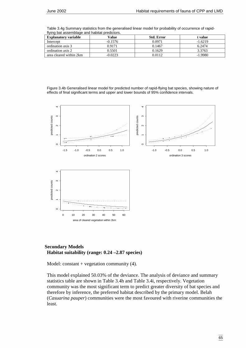
June 2002 Habitat requirements of fauna of CPP and LMD
65
Table 3.4g Summary statistics from the generalised linear model for probability of occurrence of rapid-flying bat assemblage and habitat predictors.Explanatory variable Value Std. Error t valueIntercept -0.1576 0.0971 -1.6219ordination axis 3 0.9171 0.1467 6.2474ordination axis 2 0.5501 0.1629 3.3763area cleared within 2km -0.0223 0.0112 -1.9980
Figure 3.4b Generalised linear model for predicted number of rapid-flying bat species, showing nature ofeffects of final significant terms and upper and lower bounds of 95% confidence intervals.
Secondary ModelsHabitat suitability (range: 0.24 –2.87 species)
Model: constant + vegetation community (4).
This model explained 50.03% of the deviance. The analysis of deviance and summarystatistics table are shown in Table 3.4h and Table 3.4i, respectively. Vegetationcommunity was the most significant term to predict greater diversity of bat species andtherefore by inference, the preferred habitat described by the primary model. Belah(Casuarina pauper) communities were the most favoured with riverine communities theleast.
ordination 2 scores
pred
icte
d co
unts
-1.5 -1.0 -0.5 0.0 0.5 1.0
01
23
4
ordination 3 scores
pred
icte
d co
unts
-1.0 -0.5 0.0 0.5 1.0
01
23
4
area of cleared vegetation within 2km
pred
icte
d co
unts
0 10 20 30 40 50 60
01
23
4
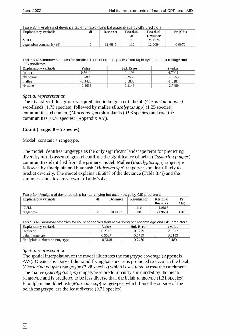
June 2002 Habitat requirements of fauna of CPP and LMD
66
Table 3.4h Analysis of deviance table for rapid-flying bat assemblage by GIS predictors.Explanatory variable df Deviance Residual
dfResidualDeviance
Pr (Chi)
NULL 113 24.1529vegetation community (4) 3 12.0845 110 12.0684 0.0070
Table 3.4i Summary statistics for predicted abundance of species from rapid-flying bat assemblage andGIS predictors.Explanatory variable Value Std. Error t valueIntercept 0.5611 0.1193 4.7001chenopod -0.5809 0.2553 -2.2753mallee -0.3420 0.1880 -1.8187riverine -0.8638 0.3143 -2.7480
Spatial representationThe diversity of this group was predicted to be greater in belah (Casuarina pauper)woodlands (1.75 species), followed by mallee (Eucalyptus spp) (1.25 species)communities, chenopod (Maireana spp) shrublands (0.98 species) and riverinecommunities (0.74 species) (Appendix AV).
Count (range: 0 – 5 species)
Model: constant + rangetype.
The model identifies rangetype as the only significant landscape term for predictingdiversity of this assemblage and confirms the significance of belah (Casuarina pauper)communities identified from the primary model. Mallee (Eucalyptus spp) rangetypefollowed by floodplain and bluebush (Maireana spp) rangetypes are least likely topredict diversity. The model explains 18.68% of the deviance (Table 3.4j) and thesummary statistics are shown in Table 3.4k.
Table 3.4j Analysis of deviance table for rapid-flying bat assemblage by GIS predictors.Explanatory variable df Deviance Residual df Residual
DeviancePr
(Chi)NULL 110 149.9813rangetype 2 28.0152 108 121.9661 0.0000
Table 3.4k Summary statistics for count of species from rapid-flying bat assemblage and GIS predictors.Explanatory variable Value Std. Error t valueIntercept 0.2719 0.1259 2.1592belah rangetype 0.5527 0.1719 3.2153floodplain + bluebush rangetype -0.6148 0.2470 -2.4891
Spatial representationThe spatial interpolation of the model illustrates the rangetype coverage (AppendixAW). Greater diversity of the rapid-flying bat species is predicted to occur in the belah(Casuarina pauper) rangetype (2.28 species) which is scattered across the catchment.The mallee (Eucalyptus spp) rangetype is predominantly surrounded by the belahrangetype and is predicted to be less diverse than the belah rangetype (1.31 species).Floodplain and bluebush (Maireana spp) rangetypes, which flank the outside of thebelah rangetype, are the least diverse (0.71 species).
June 2002 Habitat requirements of fauna of CPP and LMD
67
Summary of primary modelsAppendix AX lists the effects of the variables on the diversity of each species group.Few habitat variables were identified as predictors of bat species diversity. Ordinationaxes 2 and 3 both exhibited positive effects on diversity indicating all bat speciesdetected were associated with both mallee and belah/rosewood communities. The extentof cleared vegetation was also significant for all bat species. The greater the amount ofvegetation cleared within two kilometres of the site, the lower the predicted diversity ofbat species. Increasing structural complexity had a negative effect on the predicteddiversity of species Group 1. This group was equally composed of slow and rapid-flyingspecies and fewer species were predicted where structural complexity increased. It isreasonable to assume that more closed habitats do not favour rapid-flying species.

June 2002 Habitat requirements of fauna of CPP and LMD
68
4 DISCUSSION
This report addresses several of the project objectives stated earlier. Data from the CobarPeneplain Bioregional Assessment (Masters & Foster 2000) and the Lower Murray DarlingEnvironmental Studies (Val et al. 2001) were successfully incorporated into one databaseand preferred habitat determined. The habitat suitability of each site for every faunalassemblage was modelled as a function of the remotely mapped landscape variables andevaluated.
Analysis of the combined data set included the classification of the flora and fauna datafollowed by regression modelling to identify the local-scale habitat attributes required forspecies group diversity. Spatial models testing habitat suitability against landscapevariables and their spatial interpolation were then constructed for the Lower MurrayDarling Catchment. It was not possible to construct spatial models for the Cobar PeneplainBioregion as sufficient coverages for all variables were not available.
The identification of habitat variables at different spatial scales (local and regional) willenable the assessment of the environmental value of areas considered for various land usese.g. cultivation or reservation, particularly in relation to different faunal assemblages andwill contribute to the level of knowledge available for such programmes as the SouthernMallee Regional Guidelines for the Development of Land Use Agreements in the LowerMurray Darling Catchment (Southern Mallee Regional Planning Committee 2000).
This technical report is one of two reports specified for the project. The second is a reportthat will interpret the results of this technical report for presentation to a wider audience.That document will also present best management practices that will assist in the promotionof a greater understanding the region’s biodiversity.
4.1 ADVANCING FAUNA INVESTIGATIONS OF THE COBARPENEPLAIN BIOREGION
A recommendation of the Cobar Peneplain Bioregional Assessment, Investigating FaunaDistribution of the Cobar Peneplain (Masters & Foster 2000) was for the incorporation ofadditional survey data into the Cobar Peneplain Bioregion database. It was stressed that awider geographical spread of data would enable significant predictions of the distributionand habitat requirements of species to be obtained. As a result, fauna and flora data fromthe Lower Murray Darling biodiversity surveys were merged with the Cobar PeneplainBioregion data and the data re-analysed. Additionally, spatial models were constructed forthe Lower Murray Darling Catchment. The possibility of the development of spatial models
June 2002 Habitat requirements of fauna of CPP and LMD
69
for the peneplain may be assessed after considering the suitability of the technique and asGIS coverages for the peneplain e.g. landsystems, become available.
Assessment of fauna classification for the extended geographical rangeThe comparison of species group composition revealed a high degree of similarity betweenthe Cobar Peneplain Bioregion data set and the larger Cobar Peneplain Bioregion/LowerMurray Darling Catchment data set. The range of many species from the peneplainextended into the Lower Murray Darling catchment. However, seven resident bird species(bar-shouldered dove, black honeyeater, striated thornbill, fairy martin, yellow-facedhoneyeater, brown honeyeater and buff-rumped thornbill) recorded from Cobar PeneplainBioregion were not included in the expanded analysis due to their low occurrence. The lastthree species are uncommon visitors to the Lower Murray Darling Catchment but allspecies were recorded off-site during the Lower Murray Darling Environmental Studies. Ofthe reptile species only one species, the broad-banded sand swimmer (Eremiascincusrichardsonii) was not included in the analysis due to its low occurrence but it has beenrecorded in the catchment at off-site locations.
From the combined analysis two bird assemblages (bar-shouldered dove, buff-rumpedthornbill, western gerygone (species Group 3) and black honeyeater, brown honeyeater,dusky woodswallow, golden whistler, grey-fronted honeyeater, grey fantail, noisy friarbird,speckled warbler and shy heathwren (species Group 7)) were primarily restricted to CobarPeneplain Bioregion. One bat assemblage (little red flying fox (Pteropus scapulatus)) wasexclusive to the Cobar Peneplain Bioregion. In comparison, one bat assemblage (southernforest bat (Vespadelus regulus) and two reptile assemblages (gibber gecko (Diplodactylusbyrnei) (species Group 4)) and marbled-face delma (Delma australis), Morethia obscura,mallee dragon (Ctenophorus fordi), southern mallee striped skink (Ctenotus atlas), jewelledgecko (Diplodactylus elderi), desert skink (Egernia inornata), Murray striped skink(Ctenotus brachyonyx) (species Group 5)) were restricted to the Lower Murray DarlingCatchment. This reptile/bird dichotomy may reflect the division between reptiles in themore arid, poorer environments of the west and birds in the relatively wetter, richerenvironments of the east (Morton & James 1988, Stafford-Smith & Morton 1990).
BirdsThere was a high level of fidelity between the bird species classifications for the CobarPeneplain data set (assemblage names denoted by italics) and the combined data set.Species either remained in a similarly described assemblage or were allocated to the newgeneralist assemblage. Sixty-three percent of birds (peaceful dove, spotted bowerbird, littlefriarbird, white-plumed honeyeater and tree martin) identified as riparian species in theCobar Peneplain Bioregion study, were similarly classified in this current analysis. Two ofthe remaining three riparian species (brown honeyeater and singing honeyeater) wereidentified as belonging to the new generalist assemblage. Sixty-seven percent of openwoodland species from the Cobar Peneplain (apostlebird, yellow-throated miner, magpie-lark, blue-faced honeyeater, grey-crowned babbler and noisy miner) were aligned with thenew woodland/riparian assemblage and one of the remaining three open woodland species(white-winged chough) was placed in the new generalist assemblage. Sixty-three percent ofCobar Peneplain tall shrubland/low woodland species (inland thornbill, brown-headedhoneyeater, yellow thornbill, yellow-rumped thornbill, white-browed woodswallow,chestnut-rumped thornbill and splendid fairy-wren) were placed in the new woodlandassemblage. Four of the remaining five tall shrubland/low woodland species (weebill, red-
June 2002 Habitat requirements of fauna of CPP and LMD
70
capped robin, southern whiteface and striated pardalote) were placed in the new generalistassemblage. The majority (60%) of the Cobar Peneplain woodlands with shrub layerassemblage were allocated to the new generalist assemblage and three of the remaining fourwoodland with shrub layer species (restless flycatcher, hooded robin, black-faced cuckoo-shrike) were allocated to the new woodland assemblage. Fifty-seven percent of the CobarPeneplain mallee species assemblage (variegated fairy-wren, yellow-plumed honeyeater,white-eared honeyeater, yellow-rumped pardalote) was retained in the new malleeassemblage. The remaining three Cobar Peneplain mallee species were either not includedin the expanded analysis due to low numbers, or placed in an assemblage of infrequentlyencountered species.
ReptilesThe reptile assemblages from the Cobar Peneplain Bioregion study were predominantlygeneralists or infrequently detected species. Analysis of the expanded data set located theinfrequently detected species (eastern spiny-tailed gecko, Ctenotus allotropis, northerndtella, beaded gecko and central beared dragon) within the new reptile generalistassemblage. Ninety-two percent of the Cobar Peneplain Bioregion generalists (box-patterned gecko, beaked gecko, marbled velvet gecko, prickly gecko, tree dtella, Morethiaboulengeri, Lerista muelleri, Carnaby’s wall skink, tree skink, bearded dragon) wereretained within the new reptile generalist assemblage. The reptile assemblages from theCobar Peneplain Bioregion study had previously exhibited no environmental preferencesbut the expanded data set enabled distribution to be successfully tested against habitatvariables.
BatsWith the expanded data set, bat fauna became sufficiently abundant and widespread to beclassified and modelled.
Assessment of habitat predictors for the extended geographical rangeThe benefits of a wider geographic spread of sites become apparent when comparing thehabitat predictors of species assemblages for the Cobar Peneplain Bioregion and the speciesassemblages of the extended geographic range. More predictors of diversity were identifiedfor similar species assemblages and the percent deviance explained was generally higher.Bird species best illustrates this comparison. Vegetation community was the only predictorfor riparian bird diversity and explained 35.7% of the deviance. Modelling the expandeddata set also identified vegetation community with the addition of distance from water andvertical structural components (woodland, tall shrub and low shrub). The devianceexplained increased to 55.37%. Only vegetation community and tall shrub cover predictedthe three ‘woodland’ assemblages of the Cobar Peneplain Bioregion. By comparison, thethree ‘woodland’ assemblages of the extended geographic region identified vegetationcommunity, distance from water, vertical structural components (woodland, low shrub andground cover) and the microhabitat variables log density and cryptogam cover. Devianceexplained increased from 21 – 28.5% for the Cobar Peneplain Bioregion to 27 – 39% forthe extended region.
4.2 ASSESSMENT OF THE PRIMARY MODELS AND VARIABLES
Sixteen habitat variables were identified and in most models, more than one variable wassignificant for each group. However, the fit may have been poor (as in the case of reptile
June 2002 Habitat requirements of fauna of CPP and LMD
71
Group 5) or the range of standard errors for some models may have been wide, indicatingthe assumption of a Poisson distribution was not always correct.
4.2.1 Significant habitat variables for each faunal assemblage
Vegetation compositionVegetation floristics and/or structure were the most consistent and reliable determinants ofthe diversity of all faunal assemblages. This follows from other studies, which emphasisedthe significance of vegetation and structure in the distribution of fauna (see Bos et al.2002,Catling et al. 1998, 2000, Fox & Fox 1981) and of vegetation in assessing conservationvalue (see Margules & Nicholls 1987, Pressey et al. 1995, Pressey & Bedward 1991). Thisstudy identified the broad responses of each faunal group to vegetation thereby contributingto the knowledge of the conservation value of each community. Not suprisingly, woodlandbird species preferred woodland habitats. However, where woodland and riparian speciesoccurred together, diversity was increased by the addition of a ground cover layer and asparse low shrub layer. The riparian only bird species assemblage was also predicted toprefer woodlands with sparse low shrub cover but a tall shrub layer in place of groundcover. Vegetation composition, as opposed to structural features, was more important forbird species regarded as generalists and mallee species. Belah woodland provided a moresuitable habitat for generalist bird species and mallee spinifex communities providedsuitable habitat for mallee bird species.
Generalist reptiles were associated with sparse belah woodlands with a sparse low shrubcover. Where generalist occurred with mallee species, greater diversity could be expectedwithin mallee spinifex communities. The diversity of mallee specific species increased inmallee spinifex communities but could be expected to decline with the presence of a sparseground cover.
Bat diversity was related to both belah and mallee spinifex communities with the twoassemblages differentiated on site characteristics other than vegetation composition orstructure.
The specific vegetation requirements for each faunal group indicate that the vegetationcomposition or structural characteristics identified for one faunal assemblage may notnecessarily have been a good predictor of another assemblage; the predictor may have had anegative effect on the diversity of alternative assemblages. Conservation measurestherefore need to incorporate a range of vegetation communities and structural features tomaximise diversity across all faunal assemblages.
The conservation value of each community to the range of biological variation can also beviewed by the collective response of each faunal group to vegetation community.
Mallee/spinifex communitiesMallee/spinifex communities favoured a greater number of reptile and bat assemblages thanbird assemblages. The results of the modelling suggest that the diversity of the two largestbat assemblages (88% of total bat species) and of the two habitat specific reptileassemblages (29% of total reptile species) could be expected to increase in mallee/spinifexcommunities. The reptile results reflects the constituent species preference for mallee
June 2002 Habitat requirements of fauna of CPP and LMD
72
habitats and the survey results show that reptile species were most frequently detected onthe deep sand mallee/spinifex communities of the Lower Murray Darling Catchment.Threatened reptile species or species of concern were marbled-face delma (Delmaaustralis), Morethia obscura, mallee dragon (Ctenophorus fordi), jewelled gecko(Diplodactylus elderi) and Murray striped skink (Ctenotus brachyonyx). Bats were recordedacross all communities and frequently in mallee/spinifex communities, however, lessfrequently than in belah/rosewood communities. Bats species listed as threatened or ofregional conservation concern were little pied bat (Chalinolobus picatus), greater long-eared bat (Nyctophilus timoriensis), inland forest bat (Vespadelus baverstocki) andchocolate wattled bat (Chalinolobus morio). All bat species have previously been recordedin mallee communities (Ayers et al. 1996, Val et al. 2001) and in South Australia, thegreater long-eared bat is restricted to mallee communities (Ayres et al. 1996).
Diversity of the mallee bird assemblage was predicted to increase most in mallee/spinifexcommunities and the survey results show the species were recorded most frequently on thedeep sand mallee/spinifex communities of the Lower Murray Darling Catchment. Thisassemblage represented 9.6% of total bird species and included the threatened specieschestnut-quail thrush and Gilbert’s whistler, which have both previously been associatedwith mallee communities (Ayers et al. 1996, Val et al. 2001).
Belah/rosewood communitiesBelah/rosewood communities supported species nominated mostly as generalists. Theseincluded the two largest bat assemblages (88% of total bat species), the reptile generalists(one assemblage representing 50% of total species) and the bird generalists (oneassemblage representing 21% of total species). In this report, the term generalist has beenused to designate species that were known previously to occur in several vegetation types.The bird generalists were recorded in mulga shrubland, bimble box/red gum woodland,black box woodland, belah woodland, mallee shrublands and white cypress pine/bimblebox/red box woodland of the Cobar Peneplain and in belah woodlands and bluebushshrubland/belah woodland of the Lower Murray Darling Catchment. Reptiles were morefrequently detected in white cypress pine/bimble box/red box woodlands and mulgashrubland on the Cobar Peneplain and in belah woodland, black box woodland andbluebush shrubland/belah woodland of the Lower Murray Darling Catchment. Bats wererecorded across all communities but were most frequent in belah woodlands of the LowerMurray Darling Catchment.
The results from the modelling predict the generalist species groups to have higherdiversity in belah/rosewood communities over other communities. Several bird specieswere of conservation concern and included jacky winter, chestnut-rumped thornbill, red-capped robin, rufous whistler, crested bellbird, brown treecreeper, southern whiteface andwhite-browed treecreeper. Bats species listed as threatened were little pied bat, greaterlong-eared bat, inland forest bat and chocolate wattled bat. Belah/rosewood woodlands maytherefore be more important than other vegetation communities for listed species previouslyconsidered as generalist species.
Limitation of vegetation ordinationThe vegetation ordination scores were used as a surrogate for individual floristic speciesdata in the models, however few species were highly correlated to the axes. This is due
June 2002 Habitat requirements of fauna of CPP and LMD
73
likely to the small number of data points for some individual species. This may arise due toeither restricted distributions or widespread but sparse distributions. For example, plantspecies associated only with belah/rosewood communities of the Cobar Peneplain e.g.leopardwood (Flindersia maculosa), were not useful in describing the ordination gradients,despite being relatively common on the Cobar Peneplain. Similarly, riparian vegetationspecies such as red gum (Eucalyptus camaldulensis) are restricted to areas of favourablehabitat across the study region but do not describe the gradients. Correlations assume alinear association between the plant species and the ordination to describe a gradient andthis may not be a correct assumption for each species. A unimodal or multimodaldistribution may more accurately describe the distribution of the scarcer or restrictedspecies. Nevertheless, the ordinations gave a broad indication of vegetation communitiesacross the study area.
The limitations of the ordinations as a predictor were highlighted in the investigation ofriparian bird species. Riparian bird species were components of bird species Groups 1 and 2where belah/rosewood and mallee/spinifex communities exhibited a negative effect onspecies diversity. Riparian plant species were not highly correlated to the axes. Forexample, red gum exhibited a linear but weak association and black box (E. largiflorens)exhibited a multimodal distribution along the ordination axes. The ordination axes mayhave revealed what plant species riparian birds were not associated with but neither didthey clearly reveal what plant species they were associated with.
Vegetation integrityVegetation integrity, measured as the percentage of clearing within specified distances fromthe site of detection, impacted only upon bat diversity. However, the reliability of this resultmust be seen within the constraints of the uneven distribution of observations resultingfrom the omission of this attribute in the stratification process. Additionally, levels ofclearing will, to some extent, reflect the vegetation community in which the site waslocated with greater pressure for clearing occurring in more productive landscapes, forexample belah woodlands. Any level of clearing within two kilometres of the site reducedthe predicted number of species from both modelled groups. Their respective responsesdiffered, however. No rapid-flying species could be expected where more than 60% ofvegetation had been cleared. Only one species from the rapid and slow-flying group waspredicted to occur where more than 60% of vegetation had been cleared, representing a75% reduction in the diversity of this assemblage. Little is known of the ecology orconservation requirements of bats or the effects of vegetation fragmentation oninsectivorous bats in rural areas (Lumsden et al. 1995). However, it has been proposed thatbats are more tolerant of fragmented landscapes by virtue of their ability to fly to accessroosting sites and foraging areas. They have been known to fly large distances, more thanfive (Lunney et al. 1985) or 10 kilometres (Lumsden & Bennett 1999, Lumsden et al.1995). The key to reduced diversity possibly relates to reduced foraging and roostingopportunities. Bats are reliant on vegetation to supply invertebrates associated with foliageand for tree hollows or loose bark for roosting. The loss of these habitat resources wouldencourage large movements over the landscape in search of these requirements.
Kitchener et al. (1980) found that lizard diversity was not related to the degree of isolationfrom uncleared land. Our work suggests similar results, as the percentage of cleared landwas not a determinant of reptile diversity in general.
June 2002 Habitat requirements of fauna of CPP and LMD
74
Vegetation community extentVegetation community extent, measured as the percentage of similar vegetation communityat threshold distances from the site, had a positive but minimal influence on the predictednumber of mallee reptiles. These results must also be viewed within the limitationsdiscussed for vegetation integrity. For the mallee group, vegetation community extent wassignificant for a distance up to 500 metres from the site. The greater the extent of similarvegetation, the higher the predicted number of species from the group. The lack ofsignificance of vegetation extent for other reptile assemblages is similar to results of otherstudies conducted in buloke (Casuarina) woodlands in Victoria where patch size was notcorrelated to reptile diversity (Hadden & Westbrooke 1996).
Vegetation structural diversityVertical structural diversity was examined as the number of vegetation strata at each site.This variable was a predictor of the rapid and slow-flying bat species assemblage only,where there was a negative effect for increased structural diversity. Other studies (Foulkeset al. 1995, Hadden & Westbrooke 1996, Kitchener et al. 1980, Masters 1991, Pianka1986) have shown structural diversity to be important for reptile species diversity byproviding greater opportunities for habitat selection but was not significant in this work.
Greater vertical structural diversity is normally associated with greater bat diversity(Bennett et al. 1989). However, there is equal composition of rapid and slow-fliers in thebat assemblage for which vertical structural diversity is significant. These species feedeither on the wing on insects associated with trees and shrubs (rapid-fliers) or by gleaningfrom foliage (slow-fliers). It could be hypothesised that a more closed habitat would nothave favoured the rapid-flying species, as they are less manoeuvrable and less able to avoidobstacles such as shrubs when compared to slow-fliers. The result would be a decrease ingroup diversity as structural complexity increased. Alternatively, the result may reflect atrapping bias rather than a true effect of structural variability. In more shrubbyenvironments, locating suitable flyways for the harp trap may have been difficult; hence theopportunity for capturing species was reduced. Likewise, Anabat recordings may have beeneffected as the increased foliage may have deflected ultrasonic calls. This limitation wouldhave been exacerbated by the relatively short recording period (half an hour per site)(Richards 2001) and particularly if recording coincided with poor weather conditions suchas windy nights or low humidity.
Vegetation structural formation - woodlandComponents of vertical structural diversity i.e. structural formations, were good predictorsof species group diversity. Diversity of the woodland and riparian bird assemblage, riparianbird assemblage, woodland bird assemblage and generalist bird assemblage were allpredicted to increase with the presence of woodland. These groups exhibited differentresponses, however, with minimum numbers predicted for the woodland and riparianassemblage and greatest numbers predicted for the generalist bird assemblage. Thegeneralist reptile assemblage also preferred the presence of woodlands but group diversitywas expected to be greatest in very sparse (<10%) woodlands.
Woodland included a variety of communities spread across the study areas: belahwoodlands, black box woodlands, bimble box/red gum woodlands and white cypresspine/bimble box/red box woodlands. The association of these faunal assemblages withwoodlands conforms to known distributions (Watson et al. 2001, Simpson et al. 1999) and
June 2002 Habitat requirements of fauna of CPP and LMD
75
the work of other authors in singling out woodlands as a determinant of distribution(Kitchener et al. 1980). Several woodland bird species recorded in these surveys have beenlisted as threatened (Threatened Species Act 1995) including grey-crowned babbler, hoodedrobin and pied honeyeater. Other species of regional conservation concern were spottedbowerbird, restless flycatcher, white-browed babbler and varied sittella (NSW NPWS 2001,Val et al. 2001). Their predicted occurrence in woodlands will have implications fordevelopment and conservation strategies for the region as woodlands are often targeted fordevelopment.
Vegetation structural formation – tall shrubTall shrubs exhibited an effect only for bird species diversity. Riparian and generalist birdspecies diversity increased where tall shrubs were present and decreased where tall shrubswere absent. However, generalist species showed a greater preference for tall shrubs asmore species were predicted to occur when compared to the riparian group. Mulga (Acaciaaneura) constituted 13% of sites from the tall shrub category and 57% of species fromthese avian assemblages have been previously recorded in mulga shrublands (Recher &Davis 1997), including five species listed either as threatened or of regional conservationconcern (crested bellbird, red-capped robin, rufous whistler, southern whiteface, white-browed treecreeper).
Vegetation structural formation – low shrubThe cover of low shrubs was not a good predictor of increased fauna diversity. Thediversity of the woodland and riparian bird assemblage, the riparian bird assemblage andthe generalist reptile assemblage was greatest where cover was very sparse (<10%),indicating a preference for open habitats, but predicted numbers were low. The majority ofbirds (82% in the woodland and riparian group and 60% in the riparian only group) areknown to frequent open habitats and either forage on the ground or spend significantportions of time on the ground e.g. magpie-lark, peaceful dove, apostlebird, chestnut-crowned babbler and grey-crowned babbler (Simpson et al. 1999). Other species requireopen habitats for good vantage points from which to scan for prey on the ground e.g.laughing kookaburra, sacred kingfisher and red-backed kingfisher (Simpson et al. 1999).
The generalist reptile species also preferred habitats with an open lower stratum with 40%of species in this assemblage known to forage in open areas (Cogger 1992). Few of thesespecies were detected in deep sand mallee/spinifex sites and were more frequent in a rangeof other vegetation communities. A hummock grass understorey, common in deep sandmallee spinifex communities, may not present sufficiently open habitats for the generalistreptile species, hence reducing species diversity.
Vegetation structural fromation – ground coverGround cover had a positive effect on group diversity for the woodland and riparian birdassemblage and the mallee reptile assemblage. Ground cover incorporated several speciesbut was predominantly Chenopodiaceae dwarf shrubs (Atriplex spp and Sclerolaena spp)and mixed grassland species such as speargrasses (Austrostipa spp), wiregrasses (Aristidaspp), lovegrasses (Eragrostis spp) and mulga grass (Thyridiolepis mitchelliana). Some sitesrecorded dense cover of exotic weed species e.g. Ward’s weed (Carrichtera annua), as partof the ground cover component.
June 2002 Habitat requirements of fauna of CPP and LMD
76
Chenopod species were often dominant in riparian plant communities where woodland andriparian birds were dominant. Fifty-four percent of sites in the ground cover categoryrecorded dwarf chenopod shrubs as the ground cover. Many of these plant species areconsidered increaser species i.e. resistant to grazing or unpalatable (Wilson 1990), orcoloniser species i.e. species which establish in degraded environments (Calow 1999).Examples include streaked poverty-bush (Sclerolaena tricuspis), galvanised burr (S.muricata var. muricata), red copperburr (S. calcarata), small saltbush (Atriplex eardleyae),eastern flat-top saltbush (A. lindleyi) and slender-fruit saltbush (A. leptocarpa). Riparianzones are typically well utilised by domestic stock and high grazing pressure will produceconditions suitable for increaser and coloniser species (Cunningham et al. 1992).
The grassland species were common in mulga shrublands, bimble box/red gum woodlands,white cypress pine/ bimble box woodland and red box/white cypress pine woodlands of theCobar Peneplain. In the Lower Murray Darling Catchment, speargrass (Austrostipa spp)was common in the deep sand plain mallee/spinifex communities.
The reasons why ground cover had a positive effect on bird and reptile group diversity arenot immediately evident. Although the effect was minimal for the reptile species, for thebird species a sparse cover was predicted to result in a substantial increase in speciesdiversity. Several species of bird from the woodland and riparian group (apostlebird,crested pigeon, yellow-throated miner, magpie lark and chestnut-crowned babbler) forageon the ground for invertebrates and grass seeds and may have either fed on grass seed orinvertebrates sheltering within the ground cover. Higher amounts of ground cover mayhave decreased these open foraging opportunities. At riparian sites the high cover ofincreaser and exotic species is more likely an indicator of grazing pressure and degradedenvironments than a direct link to bird diversity. For reptiles, the presence of speargrass inmallee/spinifex communities may reflect rainfall events rather than a direct effect on reptilediversity. Reptiles found in mallee/spinifex would most likely use the shelter and foodopportunities afforded by spinifex than individual grass tussocks.
Habitat complexityHabitat complexity has been examined in several studies and identified as significant forspecies abundance and distribution for woodland bird species in northern ACT (Watson etal. 2001) and ground-dwelling small mammals in south-eastern New South Wales (Catling& Burt 1995, Catling et al. 2000). In both instances abundances were increased instructurally more complex communities. Habitat complexity scores reflect specific studylocation environments so may not be suitable for direct comparison across regions.Nevertheless, habitat complexity was significant in this work and showed that moregeneralist bird species could be expected in more structurally diverse communities. Watsonet al. (2001) examined bird 35 species, nine of them common to the generalist speciesgroup. They were brown treecreeper, grey-shrike-thrush, jacky winter, rufous whistler,southern whiteface, striated pardalote, weebill, white-winged chough and willie wagtail.Watson et al. (2001) determined that these species require, in conjunction with other habitatvariables, a minimum of a moderately complex community for a secure population. Thiscurrent study predicted the mean number of generalist bird species to be five per site, whichcorresponded to a habitat complexity score of seven. This indicates a moderate to complexstructural diversity and supports Watson’s et al. findings.
June 2002 Habitat requirements of fauna of CPP and LMD
77
Distance from waterAlthough many species of bat are known to be associated with water either for feeding orroosting opportunities within riverine vegetation (Lumsden & Bennett 1995, Young & Ford2000), this current works suggests that species distribution is equal across habitats and thatdistance from water does not influence species diversity. None of the species recorded wereknown to be exclusive to riverine habitats. However, the ability of this site characteristic toconclusively explain the diversity of bats or other assemblages may be limited due to theprocess of site selection. Stratification concentrated on selecting sites at greatest distancefrom water and was not based on equally selecting from the distance categories.
Distance from water (both natural and artificial sources) was a better predictor for birdspecies diversity, producing a variety of responses from the assemblages. Bird assemblagesthat were effected were the riparian, woodland and generalist groups. The most obviouseffect was for the riparian species with a decrease in diversity expected away from theriparian zone. Diversity for the remaining two assemblages was predicted to increase asdistance from water increased and these general trends have been noted by other authorsinvestigating the effects of water on bird abundance (Landsberg et al. 1997). Landsberg etal. (1997) found 45% of species listed in the woodland and generalist groups to decrease inabundance at sites closer to water while 30% of the riparian species were observed toincrease in abundance at such sites.
The woodland and generalists groups exhibited an inverse response to distance from water.The diversity of woodland species was expected to be higher at distances less than twokilometres from water with higher diversity of generalist species expected at distancesgreater than two kilometres. The drinking habits and diet of the constituent species canexplain the different response of these assemblages. According to ratings devised by Fisheret al. (1972) and Dominelli (1999), 60% of the riparian assemblage are considered waterdependent. That is, they require water either year round or in summer. Birds of thewoodland and generalist assemblages are considered water-independent, as theirdistribution is not related to the availability of water. Diversity of the woodland assemblagewas highest at distances less than two kilometres from water. The majority of species of theassemblage (23%) are occasional drinkers; that is, they drink when water is available. Thegeneralist bird species have the least reliance on free water and are rated as completelyindependent of water, or never seen to drink. Forty percent of the generalist species fell intothis category and the diversity of the assemblage was greatest at distances greater than twokilometres from water. If the two categories of ‘occasional’ and ‘never’ are combined, thepercentage of water-independent species rises to 38% for the woodland species and 70%for the generalists, further highlighting the water-independent behaviour of the generalists.
A strong correlation between drinking habits and diet was also noted by Fisher et al.(1972). Since different foods contain varying amounts of preformed water a diet low inpreformed water would increase a species reliance on free water. A significant proportion(40%) of the riparian species are granivorous which would necessitate water dependantdrinking habits to meet metabolic requirements and this strong affiliation was noted byFisher et al. (1972). The water-independent woodland and generalists are mostlyinsectivores (38% and 70%, respectively) for which Fisher et al. (1972) noted a strongeraffiliation with water-independent drinking habits.
June 2002 Habitat requirements of fauna of CPP and LMD
78
LogsLogs were a significant component of the preferred habitat for several groups but eachgroup exhibited different requirements. The diversity of woodland, generalist and malleebird assemblages was greater where logs were either present (for the generalist group) or ofmedium density (for woodland and mallee groups). Substantial proportions of species fromthese groups (50% of the generalist species, 77% of the woodland species and 22% of themallee species) are insectivorous and forage on the ground where logs would providesuitable foraging opportunities for birds seeking insects. The generalist reptile species werealso predicted to increase in diversity where logs were present but required higher densitiesthan required for bird species. The majority of generalist reptile species (75%) use fallentimber for either shelter e.g. tree dtella (Gehyra variegata) and Boulenger’s skink(Morethia boulengeri), or as vantage points for spotting prey e.g. central bearded dragon(Pogona vitticeps).
DisturbancesDisturbance exhibited an effect for bird species only. Disturbance was the total number ofactivities or processes regarded as detrimental to animal or plant biomass. They were eitheranthropogenic agents or ‘natural’ agents (acknowledging there may be some interactionbetween nature and land managers). Anthropogenic agents included logging, rubbishdumping, tracks and mineral extraction. ‘Natural’ agents included grazing (noting the typesof herbivores), feral animal damage, fire, erosion, exotic plant species and presence ofrabbit warrens. The number and degree of impact of each disturbance was not equal in eachvegetation community e.g. grazing by domestic stock is less intensive in malleecommunities than in belah communities, rabbits are more abundant where calcareous soilsdominate compared to sandy soils. The diversity of the mallee bird group, woodland birdgroup and generalist bird group was reduced with increasing levels of disturbance.However, the degree of response was not similar. The mallee assemblage was predicted tobe the most sensitive to disturbance and the generalist group the most resilient. At a level offive disturbances, zero mallee species were predicted to occur while one woodland speciesand four generalist species were predicted to occur for the same number of disturbances.
There is substantial literature discussing and examining the effects of habitat disturbanceand fragmentation on bird populations and diversity. This includes habitat loss fromclearing for agriculture or forestry (e.g. Ford et al. 2001, Green & Catterall 1998, Saunders& Curry 1990, Williams et al. 2001), habitat modification from changed water supplies forpastoralism or mining (e.g. Dominelli 1999, Read et al. 2000) and habitat degradation fromgrazing or over-grazing (e.g. James et al. 1995, Jansen et al. 2001, Landsberg et al. 1997,Loyn 1987, Reid & Fleming 1992). All activities have been implicated in the decline ofavian species across Australia, including the arid zone. The composition of avianassemblages has also changed as a result of these anthropogenic changes with substantialnumbers either increasing or decreasing in abundance across their range (Smith & Smith1994). This study supports others indicating a predicted decrease in diversity for mallee(Smith & Smith 1994) and woodland avian species (Briggs et al. 2001, Reid 1999).
CryptogamCryptogam cover had a positive effect on the diversity of woodland and generalist birdassemblages. Cryptogam cover is dependent upon water availability, stocking intensity, soilsurface characteristics, vegetation and soil stability, and changes to cryptogam distributionwill have flow-on effects to ecosystem processes such as nutrient recycling and plant
June 2002 Habitat requirements of fauna of CPP and LMD
79
recruitment (Hodgins & Rogers 1997, Landsberg et al. 1997). Studies have shown that hoofimpact from grazing stock will reduce cryptogam cover and this impact is greatest wherestock concentrate close to water (Andrew & Lange 1986, Eldridge & Tozer 1997, Hodginsand Rogers 1997, Landsberg et al. 1997, Lange 1969, Rogers and Lange 1971). The abovementioned bird assemblages also exhibited a positive response to distance from water, andas cryptogam cover decreases in response to stocking intensity, the value of cryptogamcover as a predictor is possibly as an indicator of reduced grazing pressure and associatedecosystem processes rather than a direct indicator of bird diversity.
The discussion above highlights the effect of local, or micro-scale, variables on individualassemblages. Variables that may determine the diversity of one faunal group may have norelation to, or have a negative impact on, alternative groups. In addition, the response ofmultiple assemblages to the same variable may differ for each level of the variable. Catling& Burt (1997) found similar results for ground-dwelling mammals in north-east NSW andconcluded that management options would differ for each group. Strategic planning forconservation management therefore needs to incorporate a wide diversity of habitats tocapture maximum fauna diversity. This requires the focus to be at a landscape level toensure capture of all spatial patterning of the micro-scale attributes, including othervariables which may not have been considered (Noss 1983, Poiani et al. 2000). Theinterpolation of the spatial models is one tool available to assist with strategic planning.
4.3 ASSESSMENT OF SECONDARY MODELS AND VARIABLES
The performance of landscape variables as surrogates of habitat suitablility was variouslysuccessful. Vegetation was a significant predictor for every faunal group and all but fourmodels. Less frequent were mean annual rainfall, landform, major rangetype and rangetype.Mean summer rainfall was not identified as a predictor for any model.
Examination of the models revealed three vegetation communities to support the greatestnumber of faunal assemblages, including a total of 15 threatened species or species ofconcern. Woodland birds, generalist reptiles and rapid and slow-flying bats were predictedto be most diverse in belah woodlands. Riverine communities were suited to generalistbirds, riparian birds and generalist reptiles.
Mallee communities provided habitat required for the mallee bird assemblage and themallee and generalist reptile assemblage, including two threatened species or species ofconcern. There was partitioning within the mallee communities between the bird and reptilefaunal groups based on rainfall with reptiles occurring in regions of lower rainfall and birdsin regions of comparatively higher rainfall. This finding supports other authors who citelower rainfall as the cause of sporadic production which favours the narrower diets ofreptiles (Pianka 1989) and reptile dispersal over bird dispersal (Morton & James 1988,Stafford-Smith & Morton 1990).
However, the models testing the habitat suitability were consistently underdispersed. Thedispersion parameter (the ratio of the residual deviance to the degrees of freedom) was lessthan 1.0. This was likely due to the high number of low prediction values and the low rangeof values. The models using the count data were better dispersed (the dispersion parameter
June 2002 Habitat requirements of fauna of CPP and LMD
80
was closer to 1.0) and either confirmed the terms identified from the model testing habitatsuitability or identified additional terms.
Half the count models identified one significant attribute and only one model identifiedthree attributes. The majority of the habitat suitability models identified only one landscapesurrogate. The small number of identified variables may be due to relatively little spatial ortemporal variation in environmental variables such as rainfall, temperature, topography andgeology across this region of NSW. For some of the faunal groups investigated, e.g.reptiles, variation in these variables may yield more influence at the micro-scale than at thelandscape-scale.
The ability of landscape variables to act as indicators of preferred habitat may be limited inthe semi-arid regions of NSW where variation in landscape attributes may be minimal.However, the process of modelling biological data against landscape variables andpredicting distributions according to the variables has been successfully employedelsewhere (NSW NPWS 1994a, 1994b). These studies were conducted in the north-east ofNSW where a greater number of environmental variables with a wider range of values wereavailable for testing than were available for the far west of NSW.
An alternative to separately modelling fauna distributions as a function of microhabitat andlandscape variables would be to incorporate both types of attributes into one data set andmodel fauna response as a function of both microhabitat and landscape attributes.Examination of deviance explained for the primary and secondary models reveals that onlythree primary models performed better than the secondary models. Even within thelimitations of the secondary models, this suggests that the remotely mapped variables canbe as successful a predictor of fauna distribution as microhabitat variables. It was assumedthat the large amount of site data presented by the microhabitat variables would lead tobetter performance in the models compared to the landscape variables and hence justifiedthe separate treatment of the attributes. The results suggest that combining the data willreveal both microhabitat variables e.g. vegetation structure, and landscape variables e.g.rainfall, that contribute to fauna distribution. This approach has been employed in otherstudies (Catling et al. 1998, Claridge & Barry 2000).
4.4 ASSESSMENT OF SPATIAL INTERPOLATION OF MODELS
The aim of the development of the spatial maps was to derive distributions of predictedspecies diversity according to suitable habitat across the catchment and in doing so, provideanother tool for the development of conservation strategies in the Lower Murray DarlingCatchment. The most immediate application of these distributions would be theirincorporation into the Southern Mallee Regional Guidelines for the Development of LandUse Agreements (Southern Mallee Regional Planning Committee 2000). The veracity ofthe maps and their value as a tool for planning however can only be substantiated throughverification (NSW NPWS 1994b, MacNally 2000). This has been used elsewhere to testmodels for selection of reserve areas (Loyn et al. 2001). This requires field surveys to beconducted in areas not sampled and the results compared with the modelled predictions. Itwould be inappropriate to employ the maps in conservation planning without testing theirreliability.
June 2002 Habitat requirements of fauna of CPP and LMD
81
The spatial interpolation for the majority of groups was based on the vegetation coverage.Six models presented maps of predicted diversity determined by the combined effects ofmore than one attribute. These maps demonstrate more successfully the application of thistechnique than maps derived from one landscape attribute.
4.5 CLEARING AS A THREAT TO BIODIVERSITY
Vegetation was significant for the diversity of all faunal groups. Clearing of nativevegetation has been listed as a threatening process under the Threatened Species Act 1995(NSW NPWS 2001) confirming that there has been a loss of native vegetation which hassignificantly impacted upon threatened species and is potentially causing other species tobecome threatened. A threatening process is defined as a process that threatens, or couldthreaten, the survival or evolution development of species, populations or ecologicalcommunities (Threatened Species Act 1995).
Clearing of native vegetation has caused widespread fragmentation of ecologicalcommunities, reduced the viability of ecological communities, resulted in habitatdestruction and loss of biological diversity and lead to soil erosion and salinity. There is anextensive amount of literature covering these topics and their consequences (e.g.Cunningham 2000, Goldney & Bowie 1990, Greig & Devonshire 1981, Lynch & Saunders1991, Sivertsen 1995).
Clearing has been identified as a threat to a number of threatened species and species thatcould become threatened. Many such species were recorded within the study region andincluded western pygmy-possum (Cercartetus concinnus), little pied bat (Chalinolobuspicatus), southern ningaui (Ningaui yvonneae), greater long-eared bat (Nyctophilustimoriensis), little red flying fox (Pteropus scapulatus), Bolam’s mouse (Pseudomysbolami), inland forest bat (Vespadelus baverstocki), swamp wallaby (Wallabia bicolor),southern bell frog (Litoria raniformis), mallee worm lizard (Aprasia inaurita), Gunther’sskink (Cyclodomorphus melanops ssp. elongata), western blue-tongued lizard (Tiliquaoccipitalis), mallee dragon (Ctenophorus fordi), Murray striped skink (Ctenotusbrachyonyx), marbled-faced delma (Delma australis), northern dtella (Gehyra dubia), piedhoneyeater (Certhionyx variegatus), chestnut quail-thrush (Cinclosoma castanotus), shyheathwren (Sericornis cautus), malleefowl (Leipoa ocellata), black-eared miner (Manorinamelanotis), barking owl (Ninox connivens), Gilbert’s whistler (Pachycephala inornata),brown treecreeper (Climacteris picumnus victoriae), hooded robin (Melanodryascucullata), grey-crowned babbler (Pomatostomus temporalis) and speckled warbler(Pyrrholaemus sagittata) (NSW NPWS 2001).
Ecological communities threatened by clearing include riparian communities and nelia(Acacia loderi) shrublands (NSW NPWS 2001).
The listing of clearing as a threatening process to biodiversity acknowledges the pressurefor alternative land uses. Clearing in the Central Division, where freehold land dominates,has generally been subjected to fewer controls than in the Western Division. In the CentralDivision portion of the Cobar Peneplain only 14% of the original woodland cover remains
June 2002 Habitat requirements of fauna of CPP and LMD
82
(Goldney and Bowie 1990). In the Lower Murray Darling Catchment portion of theWestern Division, which is leasehold land, 95% of original woodlands remain (1998 data)(LMDCMB 2001). All retained woodlands not within reserves are subject to grazing.
However, pressure on these woodlands is increasing in the Lower Murray DarlingCatchment. A recent development in land management policy for the Lower MurrayDarling Catchment is the land use agreements for Southern Mallee region. The SouthernMallee is an area in the southern region of the catchment suitable for opportunistic drylandcultivation. An agreement was reached between the South West New South Wales LandManagement Group and the Department of Land and Water Conservation whereby clearingcould be ‘traded-off’ for land set aside as conservation reserves. Since implementation ofthe plan in 1999, 37 388 hectares has been approved for clearing and 94 572 hectares setaside in private reservations (Val et al. 2002). The majority of clearing approvals are for theclearing of belah/rosewood woodlands (13 979 hectares, 37% of approvals) followed byeast-west dune mallee (7 505 hectares, 20%) and mallee mosaic, a patchy distribution ofbelah and mallee (7 714 hectares, 20%). Cleared belah/rosewood represents 25% of totalland cleared within the southern mallee region, east west dune mallee 12% and malleemosaic 7%. However, the amount of land reserved for each community does not reflect theamount cleared, creating the possibility for bias in the reserve system. Belah/rosewoodrepresents 16% of land reserved within the southern mallee region and 17% of all reservedland within the catchment. East-west dune mallee is the highest reserved vegetationcommunity within the southern mallee region (47% of reserves) and near the highestreserved community within the catchment (21% of reserves). Deep sand mallee is the mostreserved community within the catchment (22% of reserves).
A large number of threatened species and species of concern (14 birds and 6 reptiles) werepredicted to occur in woodlands across the study region. Clearly there will be a loss ofbiodiversity if actions, such as an adequate and representative network of reserves, are notestablished. The work undertaken here can assist this process in two ways. Firstly, at thelocal-scale through the identification of habitat variables related to species diversity andsecondly, at the landscape-scale by either targeting areas for reservation (areas ofpotentially highest diversity) or by excluding from consideration for clearance areas of highpredicted diversity. However, the latter option should only be achieved after verification ofthe maps as described earlier.
The regions within the catchment which have been identified as highest potential fordiversity of faunal assemblages, with the obvious exclusion of portions which have beencleared, are likely targets for conservation. However, this strategy would ignore thepotential of sub-optimal habitats to supply populations for the long-term survival ofpopulations in more favourable habitat (Barrett et al. 1994). For example, young mallee(recently burnt) is often overlooked in the selection of conservation areas compared to longunburnt (‘old growth’) mallee. Work at Tarawi Nature Reserve has shown that manyspecies such as ningaui, mallee dragon, many skink species and striated grass wren, areequally abundant in long unburnt and recently burnt mallee/spinifex habitats. In addition,young mallee/spinifex has higher vegetation species diversity than older mallee. However,this work requires clarification and further analysis and should not detract from retainingold growth vegetation (Willson, A., NSW NPWS, pers. comm., 2002). Also, studiesconducted in differing successional stages of eucalyptus forest post fire have demonstrated
June 2002 Habitat requirements of fauna of CPP and LMD
83
a sequence of fauna species replacements related to flora composition and time since fire(Fox & McKay 1981). To favour long unburnt areas would exclude those species thatpreferred earlier successional stages. The exclusion of sub-optimal habitat may alsocompromise the establishment of a fully networked system of reserves.
6 CONSERVATION MANAGEMENT IMPLICATIONS
Vegetation has been employed as an indicator of biodiversity (e.g. Ferrier & Watson 1997,Fox & Fox 1981) and as a basis for conservation planning and reserve selection through theprinciples of comprehensiveness, adequateness and representativeness (NSW NPWS 2002).This study provides further evidence of the value of vegetation and also highlights thelimitations of a strategy based on one broad-scale attribute. The requirements of all taxawere met not only from vegetation but a hierarchy of broad-scale vegetation and finer-scalesurrogates. Generalist bird species and the bat species were adapted to a range of vegetationbut others, such as mallee reptiles, mallee birds and riparian birds were specific to avegetation community and also depended on a suite of other microhabitat conditions.Large, floristically heterogenous reserves will exclude many species from protection(Pressey & Bedward 1991), therefore a conservation strategy based solely on reservingvegetation types will fail to capture the needs of a comprehensive range of fauna.Vegetation is the first level for selection but the process should be cognisant ofrequirements at other levels.
Conservation management strategies, including those incorporated in the Southern MalleeRegional Guidelines for the Development of Land Use Agreements (Southern MalleeRegional Planning Committee 2000), must also consider the scale of operation (Briggs etal. 2001, Lindenmayer 2000). Faunal assemblages have different requirements at differentscales e.g. at the local-scale bat diversity may respond to structural complexity and theamount of cleared land and at the regional scale, to vegetation community. Different faunalassemblages will also respond differently at the same scale e.g. reptile and bird diversity atthe local-scale. Therefore strategies need to incorporate a diverse range of managementscales to optimise conservation of individual faunal assemblages and arrays of differentfaunal assemblages. In practical terms this will include policies and guidelines aimed atmaintaining or improving local-scale attributes through best management practices and atthe regional scale, conserving representatives of the range of land types and vegetationcommunities.
It has been argued that the reservation of land in western NSW has been inadequate(Pressey & Taffs 2001a). These authors argue that up to 1997, reservation of land ingovernment reserves in western NSW failed to sufficiently represent the range and extentof land types and ignored the vulnerability of land types to threats such as clearing andcropping. Further work by Pressey & Taffs (2001b) measured the irreplaceability – thelikelihood that an area will be needed to contribute to conservation targets – of land types inthe western region of the state. They identified substantial portions within the LowerMurray Darling Catchment as having highest priority for protection against clearing andcropping.
June 2002 Habitat requirements of fauna of CPP and LMD
84
Local-scale habitat variables can be influenced by management practises and the resultanthabitat modification will have consequences for fauna diversity. The degree of modificationwill depend largely on land management objectives. Within the study areas, where themajority is under leasehold land tenure, the effects of human activity on fauna diversity canbe managed through best management practices. Best management practises forconservation of habitat variables may be regarded as land management practises that meetthe objectives of ecological and economic sustainability. They include policies on croppingand clearing, total grazing pressure, feral animal control, drought management and weedcontrol. These will be explored in more detail in the next scheduled report.
The implications for conservation planning developed from this project and other studiescan therefore be summarised to include:
1. Scale of faunal assemblage response –� Fauna distribution is determined by a hierarchy of broad-scale attributes, primarily
vegetation, and microhabitat attributes.� One faunal assemblage may be characterised by different habitat requirements at
the local and landscape scale.� Different faunal assemblages may exhibit varying responses to the same attribute
at the same scale.� Different faunal assemblages may exhibit varying responses to different levels of
the same attribute at the same scale.� Conservation and reservation strategies must therefore consider scale in order to
accommodate these varying responses of the faunal groups to attributes and tocapture all variation within the attribute. They should also accommodate thehierarchy of vegetation to finer-scale microhabitat attributes.
2. Distribution of faunal assemblage diversity -� The development of distribution maps for the Cobar Peneplain may be more
successful testing the recorded numbers of species in the assemblage than thepredicted number of species for the assemblage. The production of maps isdependent upon the availability of sufficient GIS coverages.
� Distribution maps of assemblage diversity in the Lower Murray DarlingCatchment must be verified before inclusion into programmes such as theSouthern Mallee Regional Guidelines for the Development of Land UseAgreements.
� Areas identified as highest diversity may be the natural choice for reserve selectionbut sub-optimal habitats i.e. areas of less diversity, should not be discounted asthese habitats will supply populations for the long-term survival of populations inmore favourable habitats and assist in establishing conservation networks.
3. Threats to faunal assemblage diversity –� The distribution maps can be used as a tool to manage the threat of clearing to
vegetation communities and associated fauna.� Clearing will impact upon the irreplaceability value of vegetation, which will alter
according to continued clearing. Irreplaceability value should influence reserveselection and should be implemented within existing programmes.

June 2002 Habitat requirements of fauna of CPP and LMD
85
� Areas of highest predicted diversity may be presently cleared and therefore unableto be included for consideration in conservation planning.
� Best management practises should be developed to maintain or improve habitatquality.

86
APPENDICES
Appendix A Vegetation data sheet used in surveys.
V E G E T A T I O N S I T E / Q U A D R A T D A T A
Site Number Date
DD MM YY
GPS
Location
Observer/s Climatic Condition 1= Wet - rainfall prior to survey, annuals present. 2 = Dry - vegetation dry, few annuals present.
Vegetation Condition 1 = virtually no cover, 2 = undisturbed natural, 3 = disturbed natural,4 = degraded natural, 5 = highly degraded
AD = Flag the dominant/codominant species for Overstorey (up to 3 spp), Emergents (up to 3 spp) and Understorey (up to 5 spp) (O/E/U).*Note: an emergent species is defined as a species that emerges above the dominant overstorey and has a cover abundance of <5% and not abundant.
CA : Cover Abundance scale adapted from Braun-Blanquet system. LS Life Stage1 = one/few individuals and <5% cover $2 = uncommon and <5% $ V = vegetative3 = common and <5% R = regenerating4 = very abundant/any number of individuals and <5% OR 5-20% D = dead/dormant5 =20-50% cover B = budding6 =50-75% of area F = flowering7 = covering more than 75% of area I = immature fruits
M = mature fruits$ where large shrubs or trees are involved upgrade the category to X = recently shed reflect the cover rather than the number of individuals S = seedling
Species CA AD0/E/U
Voucher LS/Comments
1
2
3
4
5
6
7
8
9

87
Site Number Date
DD MM YY
GPS
Location
VEGETATION ASSOCIATION DESCRIPTION (PLA)VEGETATION STRUCTURAL SUMMARY: (From highest to lowest stratum):(From observations of quadrat not plant list)
Growth Form Height(m) % o Species
VEGETATION ASSOCIATION DESCRIPTION: Dominant/Codominant overstorey species are defined as species that dominate the tallest stratumwith a canopy cover >(or equal to) 5%. If there are no layers that have a canopy cover > (or equal to) 5% then the dominant/codominant overstorey species are defined asspecies that dominate the tallest layer which has the maximum recorded cover/abundance (check plantlist). An emergent species is defined as a species that emergesabove the overstorey and occupies a stratum that has a canopy cover of less than 5%. Emergents are not part of the dominant structural layer eg. Banksia ornatashrubland with Eucalyptus arenacea. Canopy cover is based on projective foliage cover. Projective Foiliage Cover is equivalent to the percentage of shadow(compared to lght), assuming sun is straight overhead.
Overstorey Structural Description: Describe the vegetation structure, using the adapted Specth 1970 table (below), based on the averageheight of the overstorey as you view it
..............................................................................................................................................................
..........................................................................................................................................................................................................................
Life Form/Height Class Projective Foliage Cover of Tallest StratumDense (70-100%) Mid-dense (50-
70%)Mid-dense (30-50%) Sparse (10-30%) Very sparse (<10%)
Trees > 30m Tall closed forest Tall forest Tall open forest Tall woodland -Trees 10-30m Closed forest Forest Open forest Woodland Open woodlandTrees <10m Low closed forest Low forest Low open forest Low woodland Low open woodlandMallee (>3m) Closed mallee Mallee Mallee Open mallee Very open malleeLow Mallee (<3m) Closed low mallee Low mallee Low mallee Open low mallee Very open low malleeShrubs > 2m Closed scrub Scrub Open scrub Tall shrubland Tall open shrublandShrubs 0.25-2m Sclerophyllous Closed heathland Heathland Open heathland Shrubland Open shrubland Non-sclerophyllous - - Low scrubland Low shrubland Low open shrublandShrubs < 0.25m Sclerophyllous - - - Dwarf open heathland Dwarf open heathland
(fell-field) Non-sclerophyllous - - - Dwarf shrubland Dwarf open shrublandHummock grasses - - - Hummock grassland Open hummock
grasslandGraminoid (tussock)grasses
Closed grassland Grassland Grassland Open grassland Very open grassland
Sedges Closed sedgeland Sedgeland Sedgeland Open sedgeland Very open sedgelandHerbs Closed herbland Herbland Herbland Open herbland Very open herblandFerns Closed fernland Fernland Fernland - Very open fernland
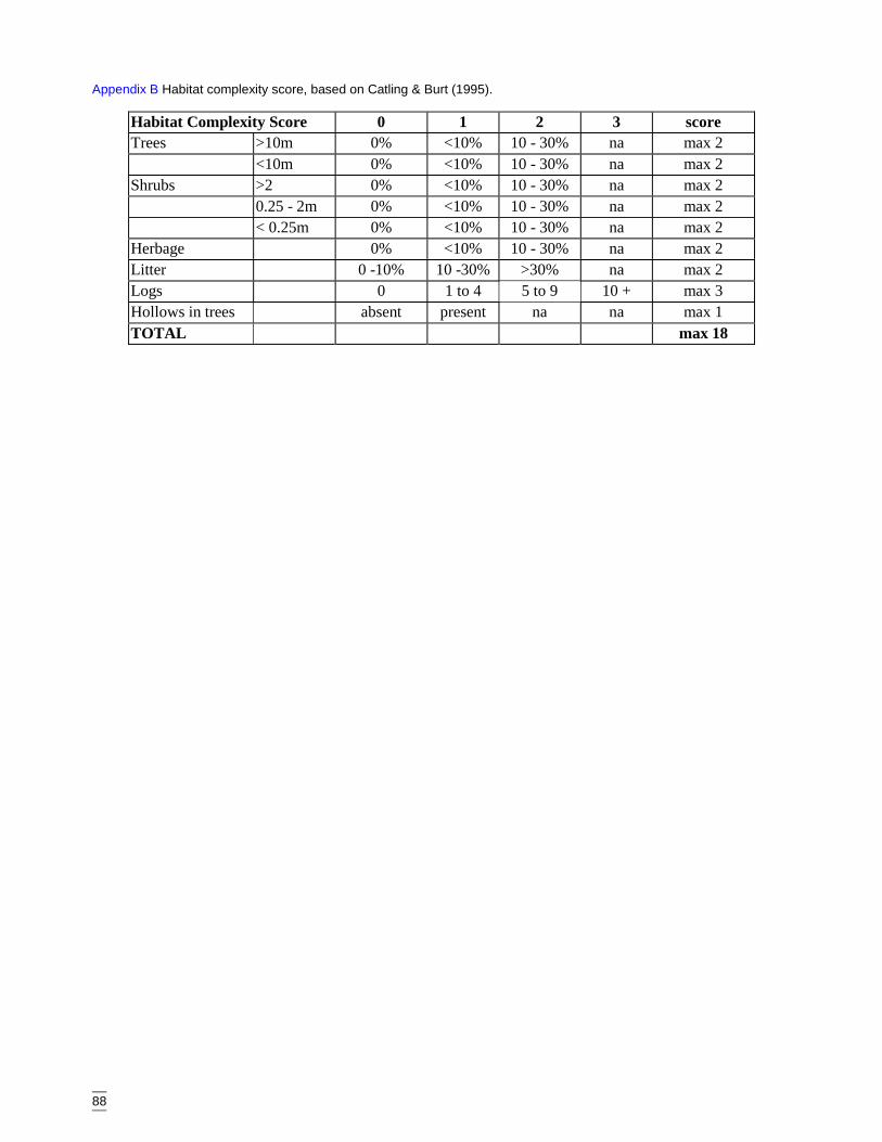
88
Appendix B Habitat complexity score, based on Catling & Burt (1995).
Habitat Complexity Score 0 1 2 3 scoreTrees >10m 0% <10% 10 - 30% na max 2
<10m 0% <10% 10 - 30% na max 2Shrubs >2 0% <10% 10 - 30% na max 2
0.25 - 2m 0% <10% 10 - 30% na max 2< 0.25m 0% <10% 10 - 30% na max 2
Herbage 0% <10% 10 - 30% na max 2Litter 0 -10% 10 -30% >30% na max 2Logs 0 1 to 4 5 to 9 10 + max 3Hollows in trees absent present na na max 1TOTAL max 18
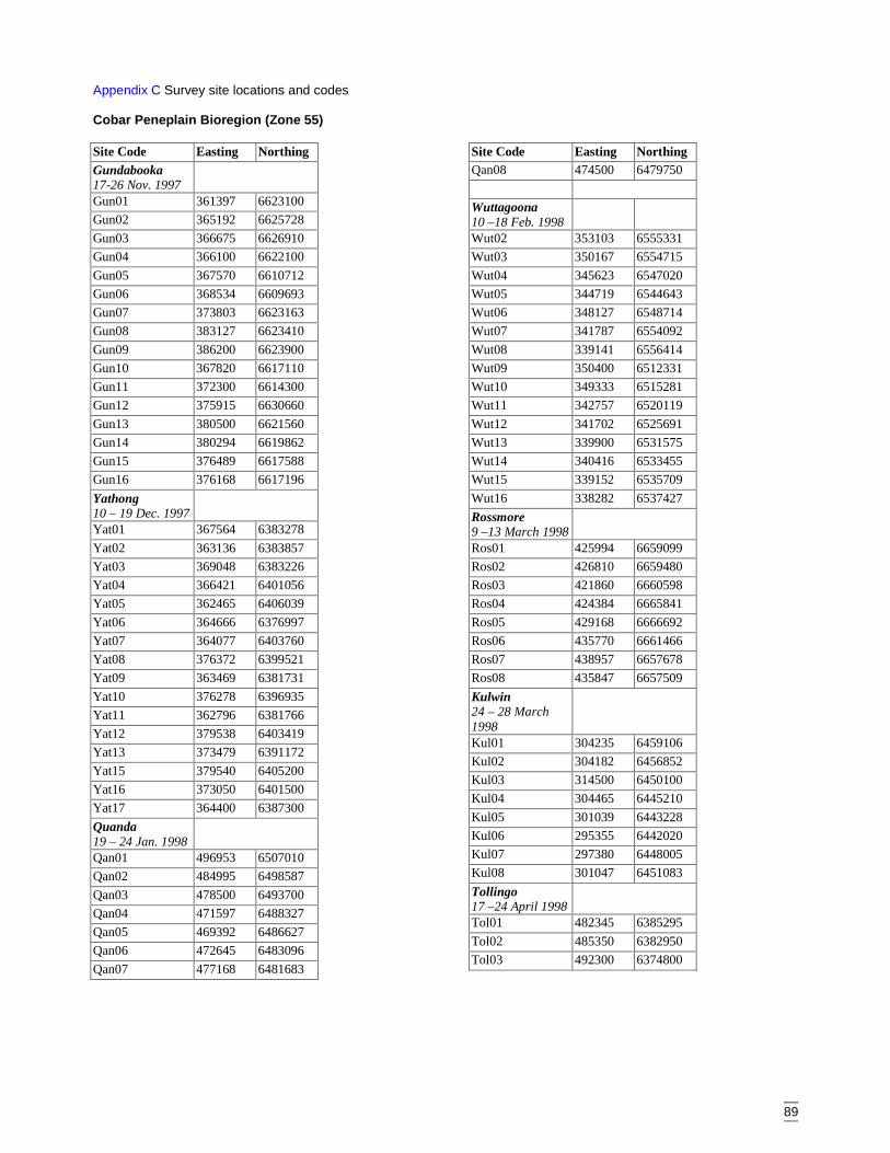
89
Appendix C Survey site locations and codes
Cobar Peneplain Bioregion (Zone 55)
Site Code Easting NorthingGundabooka17-26 Nov. 1997Gun01 361397 6623100Gun02 365192 6625728Gun03 366675 6626910Gun04 366100 6622100Gun05 367570 6610712Gun06 368534 6609693Gun07 373803 6623163Gun08 383127 6623410Gun09 386200 6623900Gun10 367820 6617110Gun11 372300 6614300Gun12 375915 6630660Gun13 380500 6621560Gun14 380294 6619862Gun15 376489 6617588Gun16 376168 6617196Yathong10 – 19 Dec. 1997Yat01 367564 6383278Yat02 363136 6383857Yat03 369048 6383226Yat04 366421 6401056Yat05 362465 6406039Yat06 364666 6376997Yat07 364077 6403760Yat08 376372 6399521Yat09 363469 6381731Yat10 376278 6396935Yat11 362796 6381766Yat12 379538 6403419Yat13 373479 6391172Yat15 379540 6405200Yat16 373050 6401500Yat17 364400 6387300Quanda19 – 24 Jan. 1998Qan01 496953 6507010Qan02 484995 6498587Qan03 478500 6493700Qan04 471597 6488327Qan05 469392 6486627Qan06 472645 6483096Qan07 477168 6481683
Site Code Easting NorthingQan08 474500 6479750
Wuttagoona10 –18 Feb. 1998Wut02 353103 6555331Wut03 350167 6554715Wut04 345623 6547020Wut05 344719 6544643Wut06 348127 6548714Wut07 341787 6554092Wut08 339141 6556414Wut09 350400 6512331Wut10 349333 6515281Wut11 342757 6520119Wut12 341702 6525691Wut13 339900 6531575Wut14 340416 6533455Wut15 339152 6535709Wut16 338282 6537427Rossmore9 –13 March 1998Ros01 425994 6659099Ros02 426810 6659480Ros03 421860 6660598Ros04 424384 6665841Ros05 429168 6666692Ros06 435770 6661466Ros07 438957 6657678Ros08 435847 6657509Kulwin24 – 28 March1998Kul01 304235 6459106Kul02 304182 6456852Kul03 314500 6450100Kul04 304465 6445210Kul05 301039 6443228Kul06 295355 6442020Kul07 297380 6448005Kul08 301047 6451083Tollingo17 –24 April 1998Tol01 482345 6385295Tol02 485350 6382950Tol03 492300 6374800
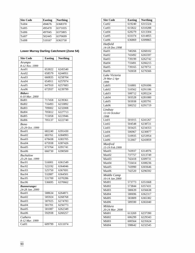
90
Site Code Easting NorthingTol04 494676 6368370Tol05 495470 6371035Tol06 497045 6375805Tol07 502445 6370699Tol08 510167 6363730
Lower Murray Darling Catchment (Zone 54)
Site Code Easting NorthingArumpo8-12 Nov. 1999Aru01 653022 6245540Aru02 658579 6244951Aru03 660835 6258704Aru04 654911 6257074Aru05 647910 6257683Aru06 672937 6239799Bidura6-10 Mar. 2000Bid01 717458 6239361Bid02 716493 6233892Bid03 709002 6232008Bid04 705812 6227713Bid05 715058 6223946Bid06 705137 6222740Bono25-29 Oct. 1999Bon01 682240 6391430Bon02 683761 6384993Bon03 678438 6383705Bon04 675938 6387426Bon05 673764 6391741Bon06 666730 6390500Buckalow25-29 Jan. 1999Buc01 516001 6361549Buc02 522192 6364046Buc03 525750 6367691Buc04 532887 6364501Buc05 531700 6370286Buc06 536695 6370662Bunnerungee24-28 Jan. 2000Bun01 588634 6264871Bun02 585924 6268768Bun03 587025 6274783Bun04 581701 6256773Bun05 581087 6262349Bun06 592938 6260257Cuthero8-12 Mar. 1999Cut01 609799 6311074
Site Code Easting NorthingCut02 619240 6315324Cut03 615822 6310288Cut04 628279 6313304Cut05 633374 6314855Cut06 636869 6309865Hatfield14-18 Dec.1998Hat01 740266 6268102Hat02 743492 6265597Hat03 739199 6262742Hat04 733491 6266215Hat05 739165 6278751Hat06 743658 6276566Lake Victoria29 Mar-2 Apr1999Lak01 516881 6291696Lak02 510562 6291186Lak03 508712 6285224Lak04 503528 6281080Lak05 503938 6285791Lak06 500252 6291719Lindsay12-16 October1998Lin01 501015 6241267Lin02 504548 6238721Lin03 503425 6234353Lin04 506967 6230877Lin05 510935 6253954Lin06 512667 6243859Manfred15-19 Feb.1999Man01 743937 6314976Man02 737757 6313749Man03 742418 6309731Man04 733414 6308236Man05 743990 6303646Man06 742520 6296592Middle Camp10-14 Jan 2000Mid01 573773 6351668Mid02 573844 6357431Mid03 580639 6356638Mid04 580696 6362317Mid05 583809 6365382Mid06 589590 6365040Mildura20-24 Mar. 2000Mld01 613269 6237390Mld02 606299 6229343Mld03 600564 6235624Mld04 598642 6232545
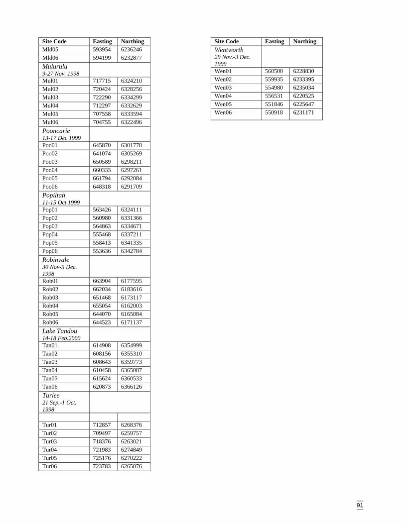
91
Site Code Easting NorthingMld05 593954 6236246Mld06 594199 6232877Mulurulu9-27 Nov. 1998Mul01 717715 6324210Mul02 720424 6328256Mul03 722290 6334299Mul04 712297 6332629Mul05 707558 6333594Mul06 704755 6322496Pooncarie13-17 Dec 1999Poo01 645870 6301778Poo02 641074 6305269Poo03 650589 6298211Poo04 660333 6297261Poo05 661794 6292084Poo06 648318 6291709Popiltah11-15 Oct.1999Pop01 563426 6324111Pop02 560980 6331366Pop03 564863 6334671Pop04 555468 6337211Pop05 558413 6341335Pop06 553636 6342784Robinvale30 Nov-5 Dec.1998Rob01 663904 6177595Rob02 662034 6183616Rob03 651468 6173117Rob04 655054 6162003Rob05 644070 6165084Rob06 644523 6171137Lake Tandou14-18 Feb.2000Tan01 614908 6354999Tan02 608156 6355310Tan03 608643 6359773Tan04 610458 6365087Tan05 615624 6360533Tan06 620873 6366126Turlee21 Sep.-1 Oct.1998
Tur01 712857 6268376Tur02 709497 6259757Tur03 718376 6263021Tur04 721983 6274849Tur05 725176 6270222Tur06 723783 6265076
Site Code Easting NorthingWentworth29 Nov.-3 Dec.1999Wen01 560500 6228830Wen02 559935 6233395Wen03 554980 6235034Wen04 556531 6220525Wen05 551846 6225647Wen06 550918 6231171
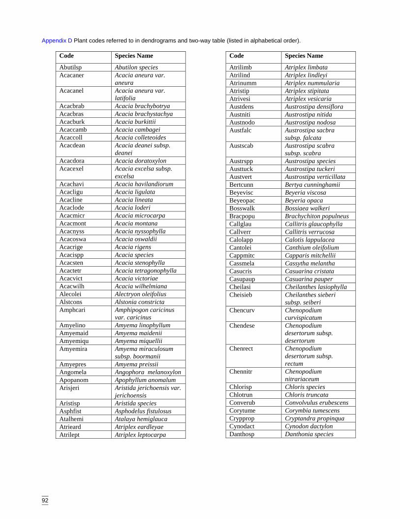
92
Appendix D Plant codes referred to in dendrograms and two-way table (listed in alphabetical order).
Code Species Name
Abutilsp Abutilon speciesAcacaner Acacia aneura var.
aneuraAcacanel Acacia aneura var.
latifoliaAcacbrab Acacia brachybotryaAcacbras Acacia brachystachyaAcacburk Acacia burkittiiAcaccamb Acacia cambageiAcaccoll Acacia colleteoidesAcacdean Acacia deanei subsp.
deaneiAcacdora Acacia doratoxylonAcacexel Acacia excelsa subsp.
excelsaAcachavi Acacia havilandiorumAcacligu Acacia ligulataAcacline Acacia lineataAcaclode Acacia loderiAcacmicr Acacia microcarpaAcacmont Acacia montanaAcacnyss Acacia nyssophyllaAcacoswa Acacia oswaldiiAcacrige Acacia rigensAcacispp Acacia speciesAcacsten Acacia stenophyllaAcactetr Acacia tetragonophyllaAcacvict Acacia victoriaeAcacwilh Acacia wilhelmianaAlecolei Alectryon oleifoliusAlstcons Alstonia constrictaAmphcari Amphipogon caricinus
var. caricinusAmyelino Amyema linophyllumAmyemaid Amyema maideniiAmyemiqu Amyema miquelliiAmyemira Amyema miraculosum
subsp. boormaniiAmyepres Amyema preissiiAngomela Angophora melanoxylonApopanom Apophyllum anomalumArisjeri Aristida jerichoensis var.
jerichoensisAristisp Aristida speciesAsphfist Asphodelus fistulosusAtalhemi Atalaya hemiglaucaAtrieard Atriplex eardleyaeAtrilept Atriplex leptocarpa
Code Species Name
Atrilimb Atriplex limbataAtrilind Atriplex lindleyiAtrinumm Atriplex nummulariaAtristip Atriplex stipitataAtrivesi Atriplex vesicariaAustdens Austrostipa densifloraAustniti Austrostipa nitidaAustnodo Austrostipa nodosaAustfalc Austrostipa sacbra
subsp. falcataAustscab Austrostipa scabra
subsp. scabraAustrspp Austrostipa speciesAusttuck Austrostipa tuckeriAustvert Austrostipa verticillataBertcunn Bertya cunninghamiiBeyevisc Beyeria viscosaBeyeopac Beyeria opacaBosswalk Bossiaea walkeriBracpopu Brachychiton populneusCallglau Callitris glaucophyllaCallverr Callitris verrucosaCalolapp Calotis lappulaceaCantolei Canthium oleifoliumCappmitc Capparis mitchelliiCassmela Cassytha melanthaCasucris Casuarina cristataCasupaup Casuarina pauperCheilasi Cheilanthes lasiophyllaCheisieb Cheilanthes sieberi
subsp. seiberiChencurv Chenopodium
curvispicatumChendese Chenopodium
desertorum subsp.desertorum
Chenrect Chenopodiumdesertorum subsp.rectum
Chennitr Chenopodiumnitrariaceum
Chlorisp Chloris speciesChlotrun Chloris truncataConverub Convolvulus erubescensCorytume Corymbia tumescensCrypprop Cryptandra propinquaCynodact Cynodon dactylonDanthosp Danthonia species
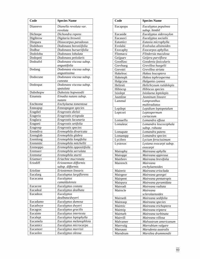
93
Code Species Name
Dianrevo Dianella revoluta var.revoluta
Dichrepe Dichondra repensDigibrow Digitaria browniiDisspara Dissocarpus paradoxusDodoboro Dodonaea boroniifoliaDodbur Dodonaea bursariifoliaDodolobu Dodonaea lobulataDodopeti Dodonaea petiolarisDodoafol Dodonaea viscosa subsp.
angustifoliaDodang Dodonaea viscosa subsp.
angustissimaDodocune Dodonaea viscosa subsp.
cuneataDodospat Dodonaea viscosa subsp.
spatulataDubohopw Duboisia hopwoodiiEinanuta Einadia nutans subsp.
nutansEnchtome Enchylaena tomentosaEnneapsp Enneapogon speciesEragdiel Eragrostis dielsiiEragerio Eragrostis eriopodaEraglacu Eragrostis lacunariaEragseti Eragrostis setifoliaEragrosp Eragrostis speciesEremdiva Eremophila divaricataEremglab Eremophila glabraEremlong Eremophila longifoliaEremmitc Eremophila mitchelliiEremoppo Eremophila oppositifoilaEremserr Eremophila serrulataEremstur Eremophila sturtiiEriamucr Eriachne mucronataEriodiff Eriostemon difformis
subsp. difformisErioline Eriostemon linearisEucalarg Eucaluptus largiflorensEucacama Eucalyptus
camaldulensisEucacost Eucalyptus costataEucadeal Eucalyptus dealbataEucadeax Eucalyptus
dealbata/dwyeriEucadumo Eucalyptus dumosaEucadwye Eucalyptus dwyeriEucagrac Eucalyptus gracilisEucainte Eucalyptus intertextaEucalept Eucalyptus leptophyllaEucamela Eucalyptus melanophloiaEucamicr Eucalyptus microcarpaEucamorr Eucalyptus morrisiiEucaoleo Eucalyptus oleosa
Code Species Name
Eucapopu Eucalyptus populneasubsp. bimbil
Eucaside Eucalyptus sideroxylonEucasoci Eucalyptus socialisEutamicr Eutaxia microphyllaEvolalsi Evolvulus alisinoidesExocaphy Exocarpos aphyllusFlinmacu Flindersia maculosaGeijparv Geijera parvifloraGoodfasc Goodenia fasicularisGrevhueg Grevillea huegeliiGrevstri Grevillea striataHakeleuc Hakea leucopteraHaketeph Hakea tephrospermaHalgcyna Halgania cyaneaHeliruti Helichrysum rutidolepisHibiscsp Hibiscus speciesIxiolept Ixiolaena leptolepisJasmline Jasminum lineareLammul Lampranthus
multiradiatusLepilept Lepidium leptopetalumLeptcori Leptospermum
coriaceumLomaeffu Lomandra effusaLomaleuc Lomandra leucocephala
subsp. robustaLomapate Lomandra patensLomanspp Lomandra speciesLycifero Lycium ferocissimumLysiexoc Lysiana exocarpi subsp.
exocarpiMairaphy Maireana aphyllaMairappr Maireana appressaMairbrev Maireana brevifoliaMairench Maireana
enchylaenoidesMaireric Maireana eriocladaMairgeor Maireana georgeiMairpent Maireana pentatropisMairpyra Maireana pyramidataMairradi Maireana radiataMairscle Maireana
sclerolaenoidesMairsedi Maireana sedifoliaMaireasp Maireana speciesMairtric Maireana trichopteraMairtrip Maireana tripteraMairturb Maireana turbinataMairvill Maireana villosaMalvamer Malvastrum americanumMarrvulg Marrubium vulgareMarsaust Marsdenia australisMarsdrum Marsilea drummondii
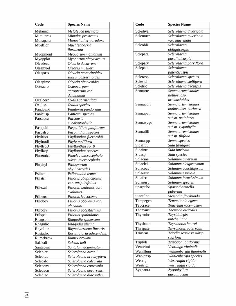
94
Code Species Name
Melaunci Melaleuca uncinataMimupros Mimulus prostratusMonapara Monachather paradoxaMuelflor Muehlenbeckia
florulentaMyopmont Myoporum montanumMyopplat Myoporum platycarpumOleadecu Olearia decurrensOleamuel Olearia muelleriOleapass Olearia passerinoides
subsp. passerinoidesOleapime Olearia pimeleoidesOsteacro Osteocarpum
acropterum var.deminutum
Oxalcorn Oxalis corniculataOxalissp Oxalis speciesPandpand Pandorea pandoranaPanicusp Panicum speciesParseuca Parsonsia
eucalyptophyllaPaspjubi Paspalidium jubiflorumPaspalsp Paspalidium speciesPhylfuer Phyllanthus fuernrohiiPhylnodi Phyla nodifloraPhyllspB Phyllanthus sp. BPhyllasp Phyllanthus speciesPimemicr Pimelea microcephala
subsp. microcephalaPittphyl Pittosporum
phylliraeoidesPsiltenu Psilocaulon tenuePtilatri Ptilotus atriplicifolius
var. atriplicifoliusPtilexal Ptilotus exaltatus var.
exaltatusPtilleuc Ptilotus leucocomaPtilobov Ptilotus obovatus var.
obovatusPtilpoly Ptilotus polystachyusPtilspat Ptilotus spathulatusRhagspin Rhagodia spinescensRhagulic Rhagodia ulicinaRhynline Rhyncharrhena linearisRostadsc Rostellularia adscendensRumebrow Rumex browniiSalskali Salsola kaliSantacum Santalum acuminatumSclebirc Sclerolaena birchiiSclebrac Sclerolaena brachypteraSclecalc Sclerolaena calcarataScleconv Sclerolaena convexulaScledecu Sclerolaena decurrensSclediac Sclerolaena diacantha
Code Species Name
Sclediva Sclerolaena divaricataSclemucr Sclerolaena mucrinata
var. mucrinataScleobli Sclerolaena
obliquicuspisSclepara Sclerolaena
parallelicuspisScleparv Sclerolaena parvifloraSclepate Sclerolaena
patenticuspisSclerosp Sclerolaena speciesSclestel Sclerolaena stelligeraScletric Sclerolaena tricuspisSennarte Senna artemisioides
nothosubsp.artemisioides
Sennacori Senna artemisioidesnothosubsp. coriacea
Sennapeti Senna artemisioidessubsp. petiolaris
Sennazygo Senna artemisioidessubsp. zygophylla
Sennafili Senna atremisioidessubsp. filifolia
Sennaspp Senna speciesSidafibu Sida fibuliferaSidaintr Sida intricataSidasp Sida speciesSolacine Solanum cinereumSolaclei Solanum cleigostemumSolacoac Solanum coactiliferumSolaesur Solanum esurialeSolafero Solanum ferocissimumSolanusp Solanum speciesSparpube Spartothamnella
puberulaStemflor Stemodia floribundaTempegen Tempeltonia egenaTeucrace Teucrium racemosumThemaust Themeda australisThyrmitc Thyridolepis
mitchellianaThysbaue Thysanotus baureiThyspate Thysanotus patersoniiTrioscar Triodia scariosa subsp.
scariosaTriploli Tripogon loliiformisVentvimi Ventilago viminalisWahlflum Wahlenbergia fluminalisWahlensp Wahlenbergia speciesWesrig Westringia rigidaWestrigi Westringia rigidaZygoaura Zygophyllum
aurantiacum
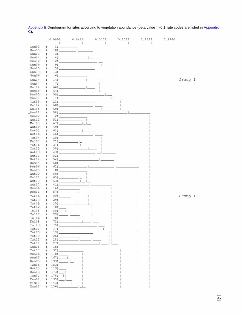
95
Appendix E Dendogram for sites according to vegetation abundance (beta value = -0.1, site codes are listed in AppendixC).
0.0092 0.0426 0.0759 0.1093 0.1426 0.1760 | | | | | | Gun01 ( 1)__________ Gun10 ( 10)_________|________ Gun03 ( 3)________________ | Gun04 ( 4)_______________|_|___ Gun12 ( 12)____________________|__ Gun09 ( 9)______________________|______ Gun05 ( 5)___________________ | Gun13 ( 13)__________________|__ | Gun06 ( 6)_______________ | | Gun14 ( 14)______________|_____|_ | Group I Gun07 ( 7)_______________ | | Kul02 ( 66)______________|____ | | Ros08 ( 64)__________________|__|___ | Ros05 ( 59)________________________|___| Gun11 ( 11)___________________________||____ Yat05 ( 21)___________________ | Kul04 ( 68)__________________|____ | Kul05 ( 69)______________________|_________|_____Ros02 ( 58)____________________________________|___________ Gun02 ( 2)_______________ | Wut11 ( 51)_____________ | | Kul03 ( 67)____________|_|__ | Wut09 ( 49)_____________ | | Ros03 ( 61)____________|___|__ | Wut06 ( 46)__________________|____ | Yat04 ( 20)___________ | | Kul07 ( 71)__________|_ | | Yat16 ( 31)___________|____ | | Yat15 ( 30)_______________|____ | | Wut03 ( 43)___________________|__|_______ | Wut12 ( 52)______________________ | | Wut14 ( 54)_____________________|_______| | Ros04 ( 60)________________ | | Ros06 ( 62)_______________|_____________|____________ | Gun08 ( 8)_______________ | | Wut10 ( 50)___________ | | | Kul01 ( 65)__________|_ | | | Wut13 ( 53)___________|__|__ | | Wut02 ( 42)________________|___________ | | Gun16 ( 16)___________ | | | Ros01 ( 57)__________|_____ | | | Yat06 ( 22)______ | | | | Group II Yat13 ( 29)_____|____ | | | | Yat09 ( 25)_________|_____|__ | | | Yat02 ( 18)____ | | | | Tol08 ( 80)___|__ | | | | Tol07 ( 79)_____|_____ | | | | Tol06 ( 78)__________|__ | | | | Kul08 ( 72)____________|____|___ | | | Tol03 ( 75)____________________|___ | | | Yat01 ( 17)_______________________|___| | | Yat03 ( 19)__________________ || | | Yat10 ( 26)___________ | || | | Yat12 ( 28)__________|______|____ || | | Yat11 ( 27)_____________________|____||___ | | Gun15 ( 15)______________________________|__ | | Yat17 ( 32)_____________ | | | Bun06 ( 110)_____ | | | | Pop03 ( 167)____|_ | | | | Wen05 ( 193)_____|__ | | | | Tan06 ( 182)_______|_ | | | | Hat03 ( 119)____ | | | | | Rob03 ( 173)___| | | | | | Tan02 ( 178)__|| | | | | | Man01 ( 135)___|___ | | | | | Mid03 ( 143)______|_|__ | | | | Man02 ( 136)__________|_|_ | | |
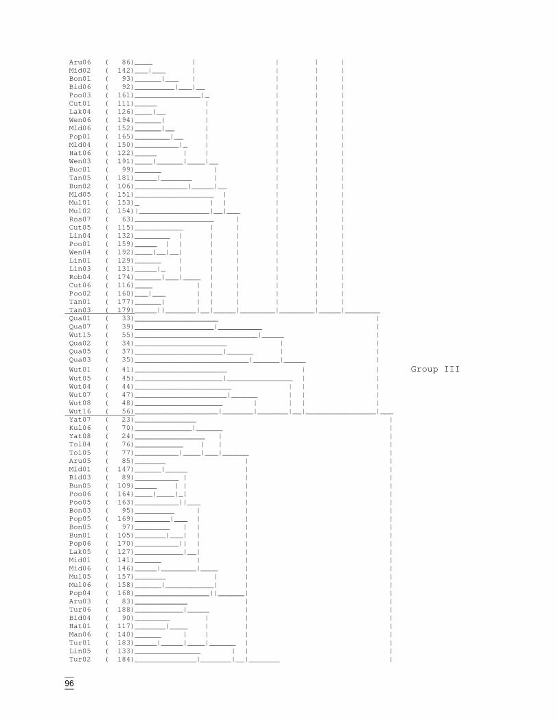
96
Aru06 ( 86)____ | | | | Mid02 ( 142)___|___ | | | | Bon01 ( 93)______|___ | | | | Bid06 ( 92)_________|___|__ | | | Poo03 ( 161)_______________|_ | | | Cut01 ( 111)_____ | | | | Lak04 ( 126)____|__ | | | | Wen06 ( 194)______| | | | | Mld06 ( 152)______|__ | | | | Pop01 ( 165)________|__ | | | | Mld04 ( 150)__________|_ | | | | Hat06 ( 122)_____ | | | | | Wen03 ( 191)____|______|____|__ | | | Buc01 ( 99)______ | | | | Tan05 ( 181)_____|_______ | | | | Bun02 ( 106)____________|_____|__ | | | Mld05 ( 151)__________________ | | | | Mul01 ( 153)_ | | | | | Mul02 ( 154)|________________|__|___ | | | Ros07 ( 63)__________________ | | | | Cut05 ( 115)___________ | | | | | Lin04 ( 132)________ | | | | | | Poo01 ( 159)_____ | | | | | | | Wen04 ( 192)____|__|__| | | | | | Lin01 ( 129)______ | | | | | | Lin03 ( 131)_____|_ | | | | | | Rob04 ( 174)______|___|____ | | | | | Cut06 ( 116)____ | | | | | | Poo02 ( 160)___|___ | | | | | | Tan01 ( 177)______| | | | | | | Tan03 ( 179)_____||_______|__|_____|________|________|_____|________ Qua01 ( 33)___________________ | Qua07 ( 39)__________________|__________ | Wut15 ( 55)____________________________|_____ | Qua02 ( 34)_____________________ | | Qua05 ( 37)____________________|______ | | Qua03 ( 35)__________________________|______|_____ | Wut01 ( 41)_____________________ | | Group III Wut05 ( 45)____________________|_______________ | | Wut04 ( 44)______________________ | | | Wut07 ( 47)_____________________|______ | | | Wut08 ( 48)____________________ | | | | Wut16 ( 56)___________________|_______|_______|__|________________|___ Yat07 ( 23)______________ | Kul06 ( 70)_____________|______ | Yat08 ( 24)________________ | | Tol04 ( 76)___________ | | | Tol05 ( 77)__________|____|___|______ | Aru05 ( 85)_______ | | Mld01 ( 147)______|_____ | | Bid03 ( 89)__________ | | | Bun05 ( 109)_____ | | | | Poo06 ( 164)____|____|_| | | Poo05 ( 163)__________||___ | | Bon03 ( 95)_________ | | | Pop05 ( 169)________|___ | | | Bon05 ( 97)________ | | | | Bun01 ( 105)_______|___| | | | Pop06 ( 170)__________|| | | | Lak05 ( 127)___________|__| | | Mid01 ( 141)______ | | | Mid06 ( 146)_____|________|____ | | Mul05 ( 157)_______ | | | Mul06 ( 158)______|___________| | | Pop04 ( 168)_________________||______| | Aru03 ( 83)____________ | | Tur06 ( 188)___________|_____ | | Bid04 ( 90)________ | | | Hat01 ( 117)_______|____ | | | Man06 ( 140)______ | | | | Tur01 ( 183)_____|_____|____|______ | | Lin05 ( 133)_______________ | | | Tur02 ( 184)______________|_______|__|_______ |
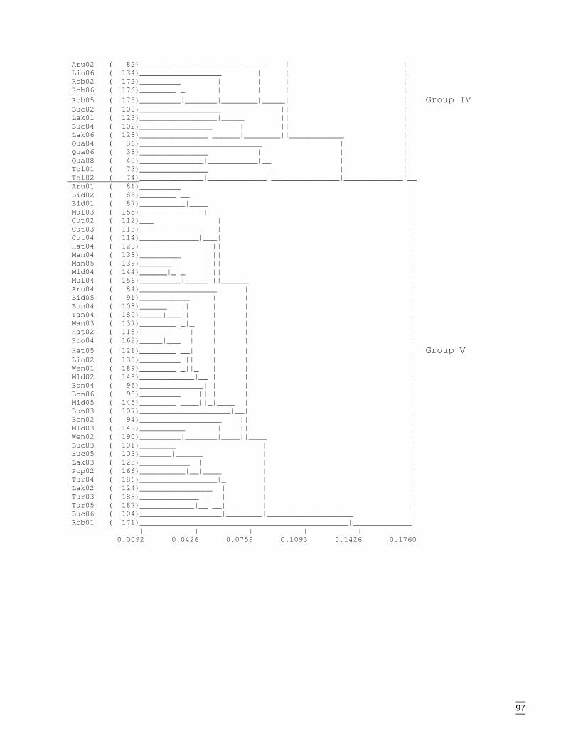
97
Aru02 ( 82)___________________________ | | Lin06 ( 134)__________________ | | | Rob02 ( 172)_________ | | | | Rob06 ( 176)________|_ | | | | Rob05 ( 175)_________|_______|________|_____| | Group IV Buc02 ( 100)__________________ || | Lak01 ( 123)_________________|_____ || | Buc04 ( 102)________________ | || | Lak06 ( 128)_______________|______|________||____________ | Qua04 ( 36)___________________________ | | Qua06 ( 38)_______________ | | | Qua08 ( 40)______________|___________|__ | | Tol01 ( 73)_______________ | | | Tol02 ( 74)______________|_____________|_______________|_____________|__ Aru01 ( 81)_________ | Bid02 ( 88)________|__ | Bid01 ( 87)__________|____ | Mul03 ( 155)______________|___ | Cut02 ( 112)___ | | Cut03 ( 113)__|___________ | | Cut04 ( 114)_____________|___| | Hat04 ( 120)________________|| | Man04 ( 138)_________ ||| | Man05 ( 139)_______ | ||| | Mid04 ( 144)______|_|_ ||| | Mul04 ( 156)_________|_____|||______ | Aru04 ( 84)_________________ | | Bid05 ( 91)___________ | | | Bun04 ( 108)______ | | | | Tan04 ( 180)_____|___ | | | | Man03 ( 137)________|_|_ | | | Hat02 ( 118)______ | | | | Poo04 ( 162)_____|___ | | | | Hat05 ( 121)________|__| | | | Group V Lin02 ( 130)_________ || | | | Wen01 ( 189)________|_||_ | | | Mld02 ( 148)____________|__ | | | Bon04 ( 96)______________| | | | Bon06 ( 98)_________ || | | | Mid05 ( 145)________|____||_|____ | | Bun03 ( 107)____________________|__| | Bon02 ( 94)__________________ || | Mld03 ( 149)__________ | || | Wen02 ( 190)_________|_______|____||____ | Buc03 ( 101)________ | | Buc05 ( 103)_______|______ | | Lak03 ( 125)___________ | | | Pop02 ( 166)__________|__|____ | | Tur04 ( 186)_________________|_ | | Lak02 ( 124)________________ | | | Tur03 ( 185)_____________ | | | | Tur05 ( 187)____________|__|__| | | Buc06 ( 104)__________________|________|___________________ | Rob01 ( 171)______________________________________________|_____________| | | | | | | 0.0092 0.0426 0.0759 0.1093 0.1426 0.1760
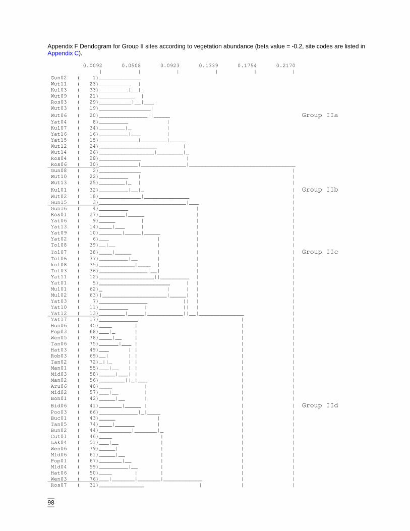
98
Appendix F Dendogram for Group II sites according to vegetation abundance (beta value = -0.2, site codes are listed inAppendix C).
0.0092 0.0508 0.0923 0.1339 0.1754 0.2170 | | | | | | Gun02 ( 1)_____________ Wut11 ( 23)__________ | Kul03 ( 33)_________|__|_ Wut09 ( 21)___________ | Ros03 ( 29)__________|__|___ Wut03 ( 19)________________| Wut06 ( 20)_______________||_____ Group IIa Yat04 ( 8)_________ | Kul07 ( 34)________|_ | Yat16 ( 16)_________|___ | Yat15 ( 15)____________|________|_____ Wut12 ( 24)__________________ | Wut14 ( 26)_________________|________|_ Ros04 ( 28)_____________ | Ros06 ( 30)____________|______________|_________________________________ Gun08 ( 2)_____________ | Wut10 ( 22)_________ | | Wut13 ( 25)________|_ | | Kul01 ( 32)_________|__|_ | Group IIb Wut02 ( 18)_____________|______________ | Gun15 ( 3)___________________________|___ | Gun16 ( 4)_________ | | Ros01 ( 27)________|_____ | | Yat06 ( 9)_____ | | | Yat13 ( 14)____|___ | | | Yat09 ( 10)_______|_____|_____ | | Yat02 ( 6)___ | | | Tol08 ( 39)__|__ | | | Tol07 ( 38)____|_____ | | | Group IIc Tol06 ( 37)_________|__ | | | kul08 ( 35)___________|____ | | | Tol03 ( 36)_______________|__| | | Yat11 ( 12)_________________||_________ | | Yat01 ( 5)______________________ | | | Mul01 ( 62)_ | | | | Mul02 ( 63)|____________________|_____| | | Yat03 ( 7)_______________ || | | Yat10 ( 11)_________ | || | | Yat12 ( 13)________|_____|___________||__|______________ | Yat17 ( 17)____________ | | Bun06 ( 45)____ | | | Pop03 ( 68)___|_ | | | Wen05 ( 78)____|__ | | | Tan06 ( 75)______|___ | | | Hat03 ( 49)___ | | | | Rob03 ( 69)__| | | | | Tan02 ( 72)_||_ | | | | Man01 ( 55)___|__ | | | | Mid03 ( 58)_____|___| | | | Man02 ( 56)________||_|___ | | Aru06 ( 40)____ | | | Mid02 ( 57)___|__ | | | Bon01 ( 42)_____|__ | | | Bid06 ( 41)_______|_____ | | | Group IId Poo03 ( 66)____________|_|____ | | Buc01 ( 43)_____ | | | Tan05 ( 74)____|______ | | | Bun02 ( 44)__________|_______|_ | | Cut01 ( 46)____ | | | Lak04 ( 51)___|__ | | | Wen06 ( 79)_____| | | | Mld06 ( 61)_____|__ | | | Pop01 ( 67)_______|__ | | | Mld04 ( 59)_________|__ | | | Hat06 ( 50)____ | | | | Wen03 ( 76)___|_______|_______|____________ | | Ros07 ( 31)______________ | | |

99
Cut05 ( 47)_________ | | | | Lin04 ( 54)_______ | | | | | Poo01 ( 64)____ | | | | | | Wen04 ( 77)___|__|_|__ | | | | Lin01 ( 52)_____ | | | | | Group IIe Lin03 ( 53)____|_ | | | | | Rob04 ( 70)_____|____|__|___ | | | Cut06 ( 48)____ | | | | Poo02 ( 65)___|__ | | | | Tan01 ( 71)_____| | | | | Tan03 ( 73)____||________ | | | | Mld05 ( 60)_____________|__|______________|____________|_______________| | | | | | | 0.0092 0.0508 0.0923 0.1339 0.1754 0.2170
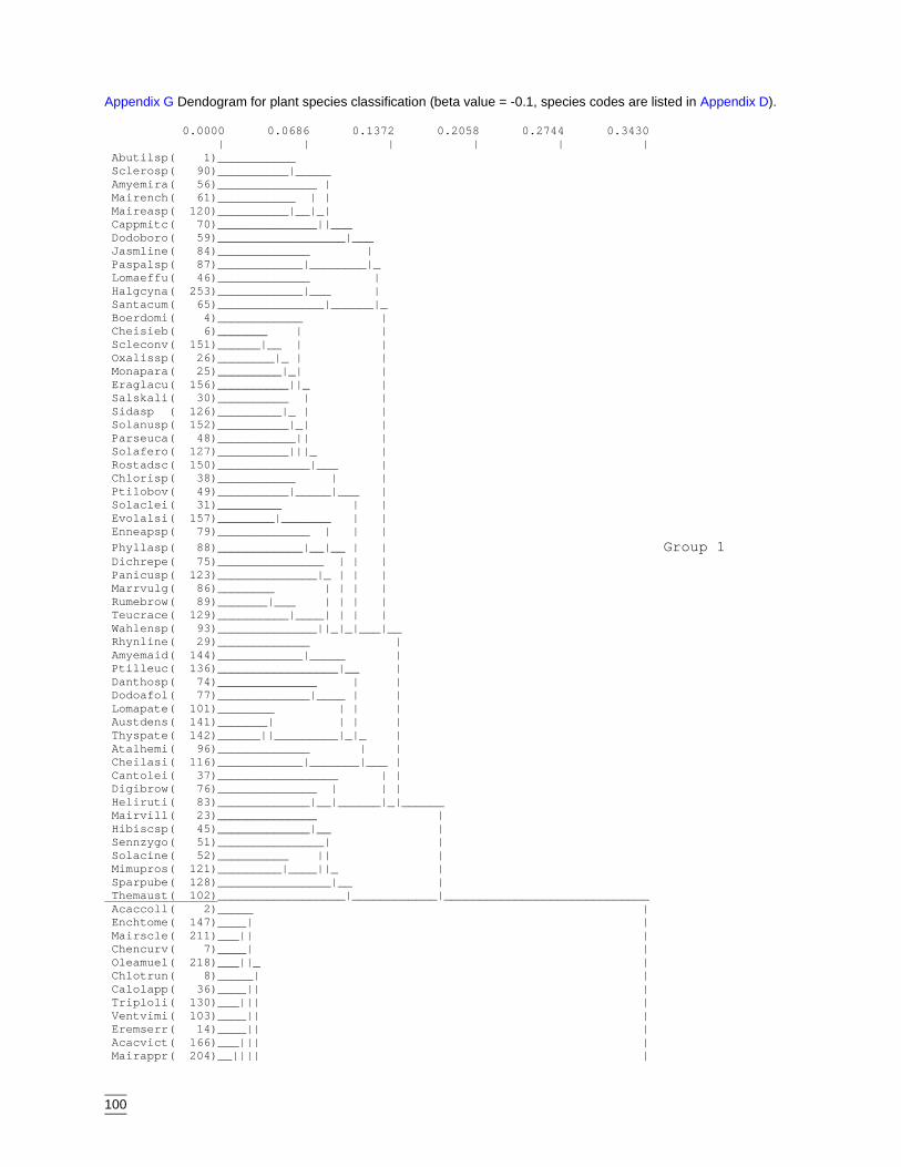
100
Appendix G Dendogram for plant species classification (beta value = -0.1, species codes are listed in Appendix D).
0.0000 0.0686 0.1372 0.2058 0.2744 0.3430 | | | | | | Abutilsp( 1)___________ Sclerosp( 90)__________|_____ Amyemira( 56)______________ | Mairench( 61)___________ | | Maireasp( 120)__________|__|_| Cappmitc( 70)______________||___ Dodoboro( 59)__________________|___ Jasmline( 84)_____________ | Paspalsp( 87)____________|________|_ Lomaeffu( 46)_____________ | Halgcyna( 253)____________|___ | Santacum( 65)_______________|______|_ Boerdomi( 4)____________ | Cheisieb( 6)_______ | | Scleconv( 151)______|__ | | Oxalissp( 26)________|_ | | Monapara( 25)_________|_| | Eraglacu( 156)__________||_ | Salskali( 30)__________ | | Sidasp ( 126)_________|_ | | Solanusp( 152)__________|_| | Parseuca( 48)___________|| | Solafero( 127)__________|||_ | Rostadsc( 150)_____________|___ | Chlorisp( 38)___________ | | Ptilobov( 49)__________|_____|___ | Solaclei( 31)_________ | | Evolalsi( 157)________|_______ | | Enneapsp( 79)_____________ | | | Phyllasp( 88)____________|__|__ | | Group 1 Dichrepe( 75)_______________ | | | Panicusp( 123)______________|_ | | | Marrvulg( 86)________ | | | | Rumebrow( 89)_______|___ | | | | Teucrace( 129)__________|____| | | | Wahlensp( 93)______________||_|_|___|__ Rhynline( 29)_____________ | Amyemaid( 144)____________|_____ | Ptilleuc( 136)_________________|__ | Danthosp( 74)______________ | | Dodoafol( 77)_____________|____ | | Lomapate( 101)________ | | | Austdens( 141)_______| | | | Thyspate( 142)______||_________|_|_ | Atalhemi( 96)_____________ | | Cheilasi( 116)____________|_______|___ | Cantolei( 37)_________________ | | Digibrow( 76)______________ | | | Heliruti( 83)_____________|__|______|_|______ Mairvill( 23)______________ | Hibiscsp( 45)_____________|__ | Sennzygo( 51)_______________| | Solacine( 52)__________ || | Mimupros( 121)_________|____||_ | Sparpube( 128)________________|__ | Themaust( 102)__________________|____________|_____________________________ Acaccoll( 2)_____ | Enchtome( 147)____| | Mairscle( 211)___|| | Chencurv( 7)____| | Oleamuel( 218)___||_ | Chlotrun( 8)_____| | Calolapp( 36)____|| | Triploli( 130)___||| | Ventvimi( 103)____|| | Eremserr( 14)____|| | Acacvict( 166)___||| | Mairappr( 204)__|||| |
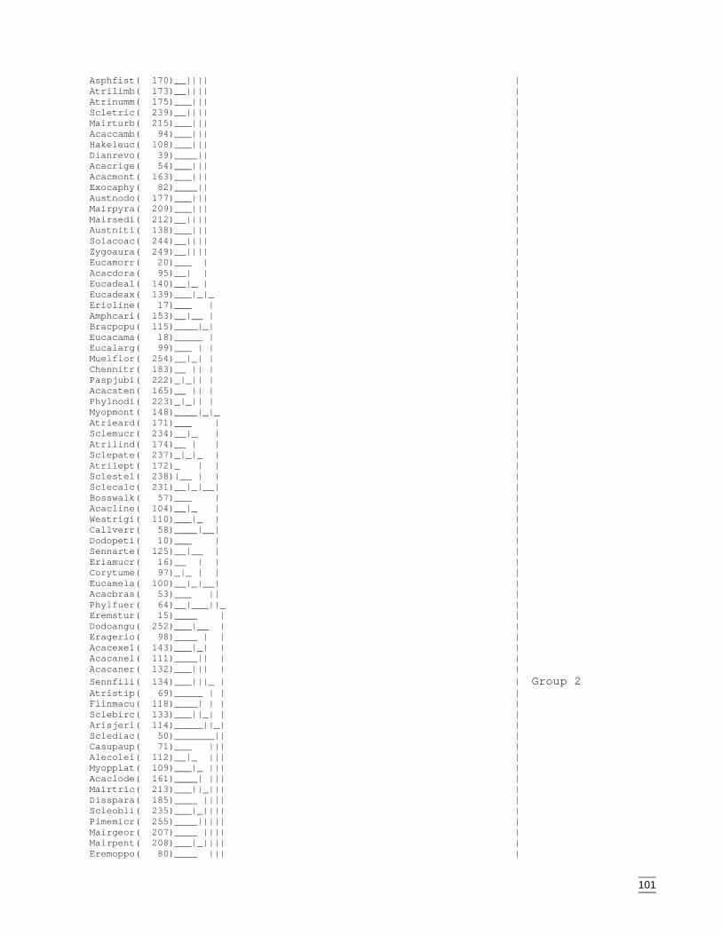
101
Asphfist( 170)__|||| | Atrilimb( 173)__|||| | Atrinumm( 175)___||| | Scletric( 239)__|||| | Mairturb( 215)___||| | Acaccamb( 94)___||| | Hakeleuc( 108)___||| | Dianrevo( 39)____|| | Acacrige( 54)___||| | Acacmont( 163)___||| | Exocaphy( 82)____|| | Austnodo( 177)___||| | Mairpyra( 209)___||| | Mairsedi( 212)__|||| | Austniti( 138)___||| | Solacoac( 244)__|||| | Zygoaura( 249)__|||| | Eucamorr( 20)___ | | Acacdora( 95)__| | | Eucadeal( 140)__|_ | | Eucadeax( 139)___|_|_ | Erioline( 17)___ | | Amphcari( 153)__|__ | | Bracpopu( 115)____|_| | Eucacama( 18)_____ | | Eucalarg( 99)___ | | | Muelflor( 254)__|_| | | Chennitr( 183)__ || | | Paspjubi( 222)_|_|| | | Acacsten( 165)__ || | | Phylnodi( 223)_|_|| | | Myopmont( 148)____|_|_ | Atrieard( 171)___ | | Sclemucr( 234)__|_ | | Atrilind( 174)__ | | | Sclepate( 237)_|_|_ | | Atrilept( 172)_ | | | Sclestel( 238)|__ | | | Sclecalc( 231)__|_|__| | Bosswalk( 57)___ | | Acacline( 104)__|_ | | Westrigi( 110)___|_ | | Callverr( 58)____|__| | Dodopeti( 10)___ | | Sennarte( 125)__|__ | | Eriamucr( 16)__ | | | Corytume( 97)_|_ | | | Eucamela( 100)__|_|__| | Acacbras( 53)___ || | Phylfuer( 64)__|___||_ | Eremstur( 15)____ | | Dodoangu( 252)___|__ | | Eragerio( 98)____ | | | Acacexel( 143)___|_| | | Acacanel( 111)____|| | | Acacaner( 132)___||| | | Sennfili( 134)___|||_ | | Group 2 Atristip( 69)_____ | | | Flinmacu( 118)____| | | | Sclebirc( 133)___||_| | | Arisjeri( 114)_____||_| | Sclediac( 50)_______|| | Casupaup( 71)___ ||| | Alecolei( 112)__|_ ||| | Myopplat( 109)___|_ ||| | Acaclode( 161)____| ||| | Mairtric( 213)___||_||| | Disspara( 185)____ |||| | Scleobli( 235)___|_|||| | Pimemicr( 255)____||||| | Mairgeor( 207)____ |||| | Mairpent( 208)___|_|||| | Eremoppo( 80)____ ||| |
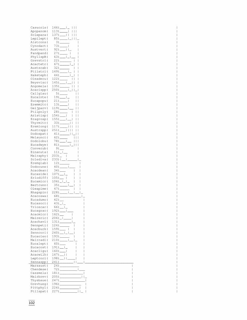
102
Casucris( 146)___|_ ||| | Apopanom( 113)____| ||| | Sclepara( 137)___|| ||| | Lepilept( 85)____|_|||_ | Alstcons( 3)_____ | | Cynodact( 73)____| | | Austvert( 92)___||_ | | Pandpand( 27)____ | | | PhyllspB( 63)___|_|__ | | Grevstri( 22)______ | | | Acactetr( 67)_____|_| | | Austscab( 32)_____ | | | Ptilatri( 149)____|_ | | | Haketeph( 44)_____|_| | | Oleadecu( 122)____ || | | Beyevisc( 145)___|__|| | | Angomela( 135)_____ || | | Acacispp( 250)____|_||_| | Callglau( 5)____ || | Eucainte( 19)___|_ || | Eucapopu( 21)____| || | Eremmitc( 13)____| || | Geijparv( 119)____|__ || | Ptilpoly( 28)____ | || | Aristisp( 154)___| | || | Eragrosp( 155)___|__| || | Thyrmitc( 33)_____|| || | Eremlong( 117)____||| || | Austrspp( 251)___|||| || | Dodospat( 41)_____||_|| | Melaunci( 62)____ ||| | Dodolobu( 78)___|__ ||| | Eucadwye( 81)_____|_||| | Converub( 9)__ | | Einanuta( 11)_|__ | | Mairaphy( 203)_ | | | Sclediva( 233)|__|_____|_ | Eremglab( 12)_____ | | Dodocune( 40)____|___ | | Acacdean( 34)___ | | | Eucaside( 107)__|_ | | | Eriodiff( 105)__ | | | | Eucamicr( 106)_|_|_ | | | Bertcunn( 35)____|__| | | Oleapime( 47)_____ | | | Rhagspin( 228)____|__|__|_ | Acacoswa( 68)___________|_ | Eucadumo( 42)__ | | Eucasoci( 43)_|_ | | Trioscar( 66)__|_ | | Eucagrac( 192)___|___ | | Acacmicr( 162)__ | | | Maireric( 206)_|____| | | Acachavi( 131)______|_ | | Sennpeti( 124)_____ | | | Acacburk( 159)___ | | | | Senncori( 240)__|_|__| | | Eucaoleo( 193)_____ | | | Mairradi( 210)____|__|_ | | Eucalept( 60)___ | | | Eucacost( 191)__|_ | | | Acacligu( 160)___| | | | Acacwilh( 167)__|| | | | Leptcori( 198)__||____| | | Sennaspp( 241)_______||___|_________________________ | Marsaust( 24)__________ | | Chendese( 72)_________|___ | | Cassmela( 181)____________| | | Mairbrev( 205)___________||_ | | Thysbaue( 247)_____________| | | Grevhueg( 196)___________ | | | Pittphyl( 224)__________| | | | Ptilspat( 227)_________||_ | | |
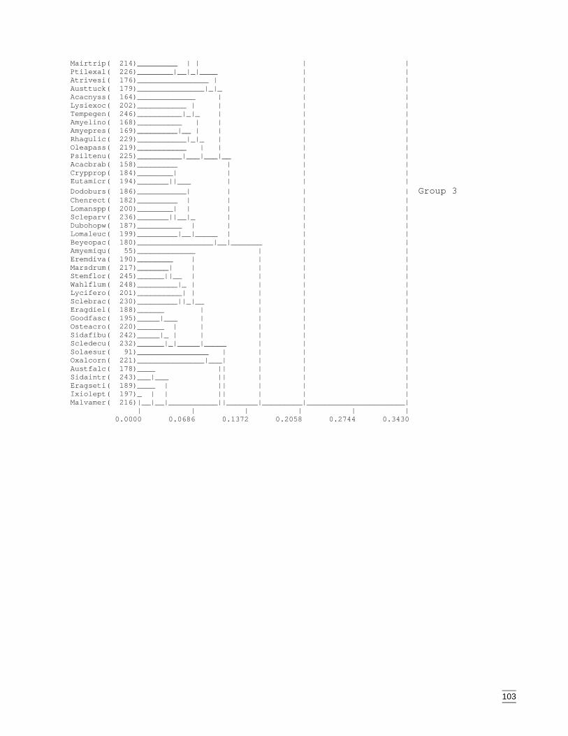
103
Mairtrip( 214)_________ | | | | Ptilexal( 226)________|__|_|____ | | Atrivesi( 176)________________ | | | Austtuck( 179)_______________|_|_ | | Acacnyss( 164)_____________ | | | Lysiexoc( 202)___________ | | | | Tempegen( 246)__________|_|_ | | | Amyelino( 168)__________ | | | | Amyepres( 169)_________|__ | | | | Rhagulic( 229)___________|_|_ | | | Oleapass( 219)___________ | | | | Psiltenu( 225)__________|___|___|__ | | Acacbrab( 158)_________ | | | Crypprop( 184)________| | | | Eutamicr( 194)_______||___ | | | Dodoburs( 186)___________| | | | Group 3 Chenrect( 182)_________ | | | | Lomanspp( 200)________| | | | | Scleparv( 236)_______||__|_ | | | Dubohopw( 187)__________ | | | | Lomaleuc( 199)_________|__|_____ | | | Beyeopac( 180)_________________|__|_______ | | Amyemiqu( 55)_____________ | | | Eremdiva( 190)________ | | | | Marsdrum( 217)_______| | | | | Stemflor( 245)______||__ | | | | Wahlflum( 248)_________|_ | | | | Lycifero( 201)__________| | | | | Sclebrac( 230)_________||_|__ | | | Eragdiel( 188)______ | | | | Goodfasc( 195)_____|___ | | | | Osteacro( 220)______ | | | | | Sidafibu( 242)_____|_ | | | | | Scledecu( 232)______|_|_____|_____ | | | Solaesur( 91)________________ | | | | Oxalcorn( 221)_______________|___| | | | Austfalc( 178)____ || | | | Sidaintr( 243)___|___ || | | | Eragseti( 189)____ | || | | | Ixiolept( 197)_ | | || | | | Malvamer( 216)|__|__|___________||_______|_________|______________________| | | | | | | 0.0000 0.0686 0.1372 0.2058 0.2744 0.3430
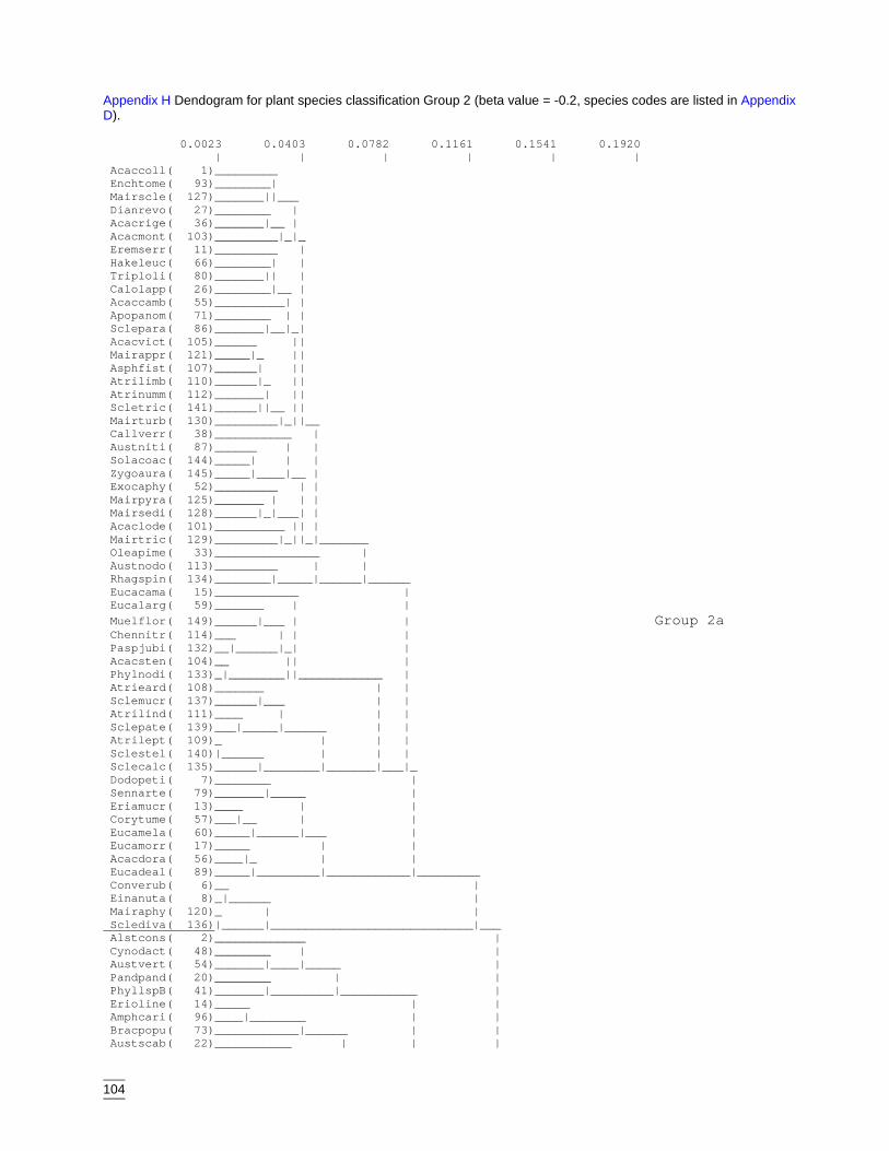
104
Appendix H Dendogram for plant species classification Group 2 (beta value = -0.2, species codes are listed in AppendixD).
0.0023 0.0403 0.0782 0.1161 0.1541 0.1920 | | | | | | Acaccoll( 1)_________ Enchtome( 93)________| Mairscle( 127)_______||___ Dianrevo( 27)________ | Acacrige( 36)_______|__ | Acacmont( 103)_________|_|_ Eremserr( 11)_________ | Hakeleuc( 66)________| | Triploli( 80)_______|| | Calolapp( 26)________|__ | Acaccamb( 55)__________| | Apopanom( 71)________ | | Sclepara( 86)_______|__|_| Acacvict( 105)______ || Mairappr( 121)_____|_ || Asphfist( 107)______| || Atrilimb( 110)______|_ || Atrinumm( 112)_______| || Scletric( 141)______||__ || Mairturb( 130)_________|_||__ Callverr( 38)___________ | Austniti( 87)______ | | Solacoac( 144)_____| | | Zygoaura( 145)_____|____|__ | Exocaphy( 52)_________ | | Mairpyra( 125)_______ | | | Mairsedi( 128)______|_|___| | Acaclode( 101)__________ || | Mairtric( 129)_________|_||_|_______ Oleapime( 33)_______________ | Austnodo( 113)_________ | | Rhagspin( 134)________|_____|______|______ Eucacama( 15)____________ | Eucalarg( 59)_______ | | Muelflor( 149)______|___ | | Group 2a Chennitr( 114)___ | | | Paspjubi( 132)__|______|_| | Acacsten( 104)__ || | Phylnodi( 133)_|________||____________ | Atrieard( 108)_______ | | Sclemucr( 137)______|___ | | Atrilind( 111)____ | | | Sclepate( 139)___|_____|______ | | Atrilept( 109)_ | | | Sclestel( 140)|______ | | | Sclecalc( 135)______|________|_______|___|_ Dodopeti( 7)________ | Sennarte( 79)_______|_____ | Eriamucr( 13)____ | | Corytume( 57)___|__ | | Eucamela( 60)_____|______|___ | Eucamorr( 17)_____ | | Acacdora( 56)____|_ | | Eucadeal( 89)_____|_________|____________|_________ Converub( 6)__ | Einanuta( 8)_|______ | Mairaphy( 120)_ | | Sclediva( 136)|______|_____________________________|___ Alstcons( 2)_____________ | Cynodact( 48)________ | | Austvert( 54)_______|____|_____ | Pandpand( 20)________ | | PhyllspB( 41)_______|_________|___________ | Erioline( 14)_____ | | Amphcari( 96)____|________ | | Bracpopu( 73)____________|______ | | Austscab( 22)___________ | | |
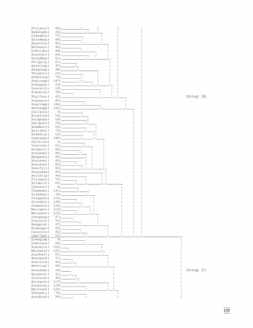
105
Ptilatri( 95)__________|___ | | | Haketeph( 32)_____________|____|__ | | Oleadecu( 77)___________ | | | Eucadeax( 88)__________| | | | Beyevisc( 91)__________|_________|___ | | Melaunci( 40)__________ | | | Dodolobu( 49)_________|________ | | | Acactetr( 44)______________ | | | | Eucadwye( 51)_____________|___|_____|_ | | Ptilpoly( 21)________ | | | Aristisp( 97)_______|_ | | | Eragrosp( 98)________|__________ | | | Thyrmitc( 23)___________ | | | | Eremlong( 74)__________| | | | | Austrspp( 147)_________||_____ | | | | Dodospat( 29)_______________|__|_____|_ | | Grevstri( 19)____________________ | | | Acacbras( 35)______ | | | | Phylfuer( 42)_____|_____________|_____|__|____ | Group 2b Angomela( 85)____________ | | Acacispp( 146)___________|________ | | Sennaspp( 143)___________________|____________|____ | Callglau( 3)___________ | | Eucainte( 16)__________|___ | | Eucapopu( 18)_____________| | | Geijparv( 76)____________||____ | | Eremmitc( 10)_____________ | | | Arisjeri( 72)____________|____| | | Eremstur( 12)___________ || | | Dodoangu( 148)__________|_____||____ | | Chlotrun( 5)____________ | | | Ventvimi( 61)___________|____ | | | Eragerio( 58)__________ | | | | Acacexel( 90)_________|___ | | | | Myopmont( 94)____________| | | | | Acacanel( 69)________ | | | | | Acacaner( 82)_______|___ | | | | | Sennfili( 84)__________|_|__|_____|_ | | Acacoswa( 45)_____________________ | | | Atristip( 46)_____________ | | | | Flinmacu( 75)________ | | | | | Sclebirc( 83)_______|____|_______|_|________ | | Chencurv( 4)_________ | | | Oleamuel( 131)________|_____ | | | Sclediac( 34)_____________|___ | | | Disspara( 115)________ | | | | Scleobli( 138)_______|___ | | | | Pimemicr( 150)__________|____ | | | | Mairgeor( 123)________ | | | | | Mairpent( 124)_______|______|_|__ | | | Casupaup( 47)______ | | | | Alecolei( 70)_____|____ | | | | Myopplat( 67)_________|________|_____ | | | Eremoppo( 50)__________ | | | | Casucris( 92)_________|___ | | | | Lepilept( 53)____________|__________|______|_____|___|____________________ Eremglab( 9)____________ | Dodocune( 28)___________|_________ | Acacmicr( 102)____ | | Maireric( 122)___|________________|_ | Acachavi( 81)_____________________|__ | Bosswalk( 37)______ | | Acacline( 62)_____|__ | | Westrigi( 68)_______|_______________|___ | Eucadumo( 30)_____ | | Group 2c Eucasoci( 31)____|___ | | Trioscar( 43)_______|_ | | Eucagrac( 117)________|_______________ | | Eucaoleo( 118)_____________ | | | Mairradi( 126)____________|__________|__|__ | Sennpeti( 78)_____________ | | Acacburk( 99)______ | | |
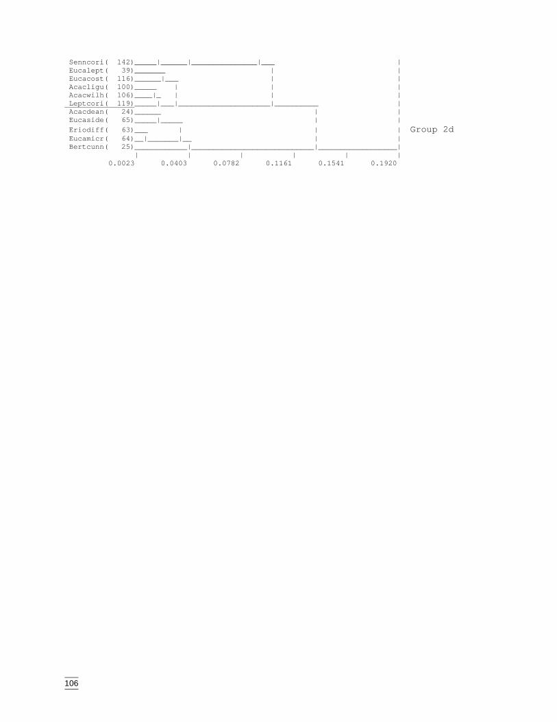
106
Senncori( 142)_____|______|_______________|___ | Eucalept( 39)_______ | | Eucacost( 116)______|___ | | Acacligu( 100)_____ | | | Acacwilh( 106)____|_ | | | Leptcori( 119)_____|___|_____________________|__________ | Acacdean( 24)______ | | Eucaside( 65)_____|_____ | | Eriodiff( 63)___ | | | Group 2d Eucamicr( 64)__|_______|__ | | Bertcunn( 25)____________|____________________________|__________________| | | | | | | 0.0023 0.0403 0.0782 0.1161 0.1541 0.1920
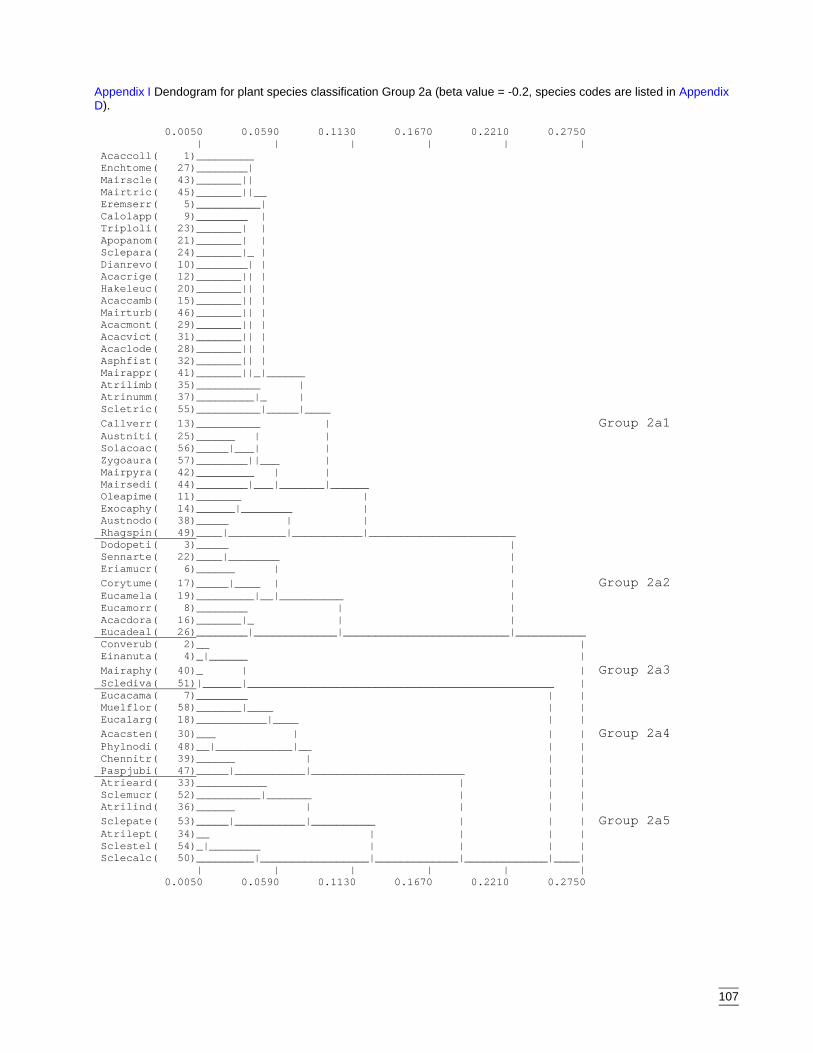
107
Appendix I Dendogram for plant species classification Group 2a (beta value = -0.2, species codes are listed in AppendixD).
0.0050 0.0590 0.1130 0.1670 0.2210 0.2750 | | | | | | Acaccoll( 1)_________ Enchtome( 27)________| Mairscle( 43)_______|| Mairtric( 45)_______||__ Eremserr( 5)__________| Calolapp( 9)________ | Triploli( 23)_______| | Apopanom( 21)_______| | Sclepara( 24)_______|_ | Dianrevo( 10)________| | Acacrige( 12)_______|| | Hakeleuc( 20)_______|| | Acaccamb( 15)_______|| | Mairturb( 46)_______|| | Acacmont( 29)_______|| | Acacvict( 31)_______|| | Acaclode( 28)_______|| | Asphfist( 32)_______|| | Mairappr( 41)_______||_|______ Atrilimb( 35)__________ | Atrinumm( 37)_________|_ | Scletric( 55)__________|_____|____ Callverr( 13)__________ | Group 2a1 Austniti( 25)______ | | Solacoac( 56)_____|___| | Zygoaura( 57)________||___ | Mairpyra( 42)_________ | | Mairsedi( 44)________|___|_______|______ Oleapime( 11)_______ | Exocaphy( 14)______|________ | Austnodo( 38)_____ | | Rhagspin( 49)____|_________|___________|_______________________ Dodopeti( 3)_____ | Sennarte( 22)____|________ | Eriamucr( 6)______ | | Corytume( 17)_____|____ | | Group 2a2 Eucamela( 19)_________|__|__________ | Eucamorr( 8)________ | | Acacdora( 16)_______|_ | | Eucadeal( 26)________|_____________|__________________________|___________ Converub( 2)__ | Einanuta( 4)_|______ | Mairaphy( 40)_ | | Group 2a3 Sclediva( 51)|______|________________________________________________ | Eucacama( 7)________ | | Muelflor( 58)_______|____ | | Eucalarg( 18)___________|____ | | Acacsten( 30)___ | | | Group 2a4 Phylnodi( 48)__|____________|__ | | Chennitr( 39)______ | | | Paspjubi( 47)_____|___________|________________________ | | Atrieard( 33)___________ | | | Sclemucr( 52)__________|_______ | | | Atrilind( 36)______ | | | | Sclepate( 53)_____|___________|__________ | | | Group 2a5 Atrilept( 34)__ | | | | Sclestel( 54)_|________ | | | | Sclecalc( 50)_________|_________________|_____________|_____________|____| | | | | | | 0.0050 0.0590 0.1130 0.1670 0.2210 0.2750
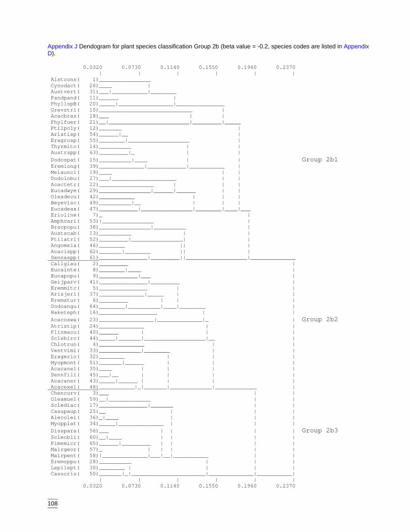
108
Appendix J Dendogram for plant species classification Group 2b (beta value = -0.2, species codes are listed in AppendixD).
0.0320 0.0730 0.1140 0.1550 0.1960 0.2370 | | | | | | Alstcons( 1)________________ Cynodact( 26)____ | Austvert( 31)___|___________|________ Pandpand( 11)______ | PhyllspB( 20)_____|_________________|_______________ Grevstri( 10)_____________________________ | Acacbras( 18)___ | | Phylfuer( 21)__|_________________________|_________|_____ Ptilpoly( 12)_______ | Aristisp( 54)______|__ | Eragrosp( 55)________|___________________ | Thyrmitc( 14)__________ | | Austrspp( 63)_________|_ | | Dodospat( 15)__________|____ | | Group 2b1 Eremlong( 39)______________|____________|___________ | Melaunci( 19)____ | | Dodolobu( 27)___|____________________ | | Acactetr( 22)_________________ | | | Eucadwye( 29)________________|______|______ | | Oleadecu( 42)___________ | | | Beyevisc( 49)__________|__ | | | Eucadeax( 47)____________|________________|________|____|___ Erioline( 7)_ | Amphcari( 53)|________________ | Bracpopu( 38)________________|__________ | Austscab( 13)__________ | | Ptilatri( 52)_________|________________| | Angomela( 46)________ || | Acacispp( 62)_______|________ || | Sennaspp( 61)_______________|_________||___________________|______________ Callglau( 2)_________ | Eucainte( 8)________|____ | Eucapopu( 9)____________|___ | Geijparv( 41)_______________|_________ | Eremmitc( 5)_______________ | | Arisjeri( 37)______________|_____ | | Eremstur( 6)_________ | | | Dodoangu( 64)________|__________|____|________ | Haketeph( 16)__________________ | | Acacoswa( 23)_________________|______________|_ | Group 2b2 Atristip( 24)______________ | | Flinmacu( 40)______ | | | Sclebirc( 44)_____|_______|___________________|__ | Chlotrun( 4)______________ | | Ventvimi( 33)_____________|________ | | Eragerio( 32)________ | | | Myopmont( 51)_______|______ | | | Acacanel( 35)____ | | | | Sennfili( 45)___|__ | | | | Acacaner( 43)_____|______ | | | | Acacexel( 48)___________|_|_______|_____________|_____________ | Chencurv( 3)___ | | Oleamuel( 59)__|_____________ | | Sclediac( 17)_______________|_______ | | Casupaup( 25)__ | | | Alecolei( 36)_|____ | | | Myopplat( 34)_____|______________ | | | Disspara( 56)___ | | | | Group 2b3 Scleobli( 60)__|____ | | | | Pimemicr( 65)______|_________ | | | | Mairgeor( 57)_ | | | | | Mairpent( 58)|______________|___|__|___________ | | Eremoppo( 28)__________ | | | Lepilept( 30)________ | | | | Casucris( 50)_______|_|_______________________|______________|___________| | | | | | | 0.0320 0.0730 0.1140 0.1550 0.1960 0.2370
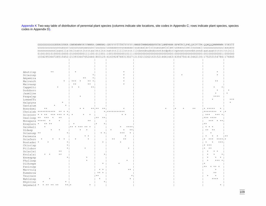
109
Appendix K Two-way table of distribution of perennial plant species (columns indicate site locations, site codes in Appendix C; rows indicate plant species, speciescodes in Appendix D).
GGGGGGGGGGGKRRGYKKR|GWKWRWWYKYYWWRR|GWWKWG|GRYYYYTTTKTYYYYY|MMHRTMMMAMBBPBTBCLWMPMHW|BPWTRCLPWLLRCPTTM|QQWQQQWWWWWW|YYKYTT uuuuuuuuuuuuoouauuo|uuuuouuauaauuoo|uuuuuu|uoaaaaooouoaaaaa|uuaoaaiarioiouauuaelolae|uoeaouioeiiouoaal|uuuuuuuuuuuu|aauaoo nnnnnnnnnnnlssntlls|ntltstttlttttss|nttltn|nsttttlllllttttt|lltbnndnudndocnntkndpdtn|npnnstnonnnbtonnd|aataaatttttt|ttltll 0100100101000010000|010000000111100|011001|1001000000010111|000000000000000000000000|00000000000000000|001000000001|000000 1034295364728515452|213933647652446|803125|6163928768313027|213321326216315214661463|63567541413462135|175253154786|176845 | | | | | | | | | | | | | | | | | | | | | | | | | | | | Abutilsp ** | * | | * | | | * | Sclerosp | *| | * | | * | * | Amyemira | ** *| | * | | | | Mairench * | *** * ** *| | * | | | ** | Maireasp | ** ** | | * | | | | Cappmitc * | * * **| | | | | * *| Dodoboro | | | | | | * | * Jasmline | | | | | | * | * Paspalsp | * | | | | | **** | Lomaeffu | | | | | | * | *** Halgcyna * | | | | | | | * Santacum * * | | | | | | | Boerdomi ** | * * **|** **| * | * |* * ** |* ***** * | Cheisieb *********** ** * *| | *|*********** | | |******** * |* Scleconv * * ** *** *** * *| * * * | | * * | | | *** *** *| Oxalissp ** *** * ** | |** **| | | |*** **** | Monapara ***** * * | ** | | | | | *** * **| Eraglacu * ** ** | * |* *| | | |** | Salskali * |** * *** ** * | | * ****| | | * * * | Sidasp * * | * * | | * * **| | | ** ** | Solanusp ** *| | * *| *** * | | | * | Parseuca | * * | | * | | | * * * |** Solafero * * * * | * * | | ** ** | | |* *** ****|* Rostadsc * * *| | * | * | | | * * ***| Chlorisp *| | | | | |* *** | Ptilobov *| * | | * | | |* ** | Solaclei ** | | | | | | * * * | Evolalsi * * ** | | *| | | | * * *| Enneapsp *| * | | | | | * * * | Phyllasp | * | | * | | | * *** *| Dichrepe | | * | * | | |* | Panicusp | | | | | |** * ** * | Marrvulg | | * * | ** | | | * | Rumebrow | | ** * | | | | ** | Teucrace | |** | *| | | * * | Wahlensp * | | * | * | | | **** | Rhynline * * | | *| | | | | Amyemaid * * ** ** ** **|* * | | | | | * |

110
Ptilleuc * * | | | | | | | * Danthosp | | | * * * | | |* * | * Dodoafol * | | | | | | * | * Lomapate | | | * ** | | | | Austdens | | | *** * | | | | Thyspate | | | * * | | | |* Atalhemi *| **| | | | | | Cheilasi * *| | | * | | | | Cantolei | | | | | |** * | Digibrow | | | * | | | ** | Heliruti * | | | | | | **| Mairvill ** | | | | | | ** | Hibiscsp * | | | | | | * | Sennzygo | | | | | |* * * | Solacine | | | | | | * ** | Mimupros | | * | | | |* * | Sparpube * * | | | | | | * | Themaust *| | | * | | | * | -------------------+---------------+------+----------------+------------------------+-----------------+------------+------ Acaccoll * | * | | | | | ** * | * Enchtome * |* *** * | | | * ** 3 * *** **| * * *| | Mairscle | | | | * ** *| | | Mairtric | | | | | | | Eremserr 1 | | * | | | | |* Calolapp | | 4 | | | | * * *** * *| Triploli *** ***** * * | ** * * | | 3 * * | | |* * * *| Apopanom |*3* ** * **| * | | | |* * | Sclepara * * |1 | | | | | | Dianrevo | | | * | | | * | *3** Acacrige | | | | | | | * ** Hakeleuc | | | 1 | 1 | | | * Acaccamb | 5 | | | | | | Mairturb | | | | | | | Acacmont | | | | | | | Acacvict | | | | 1 | | | Acaclode | | | | | | | Asphfist | | | | 4 | * | | Mairappr | | | |55 * | | | Atrilimb | | | | * | 3 ** | | Atrinumm | | | | | 5 | | Scletric | | | | | 4*** *| | Callverr | | | | 2 | | | * 1* Austniti * * * | | | | 3** 4 *5 ** 44|* | | Solacoac | | | | 4 | | | Zygoaura | | | | 5 | | | Mairpyra | | | | 5*545555| | | Mairsedi | | | | *5* * *4| | | Oleapime | | | | * | |* | * * Exocaphy | * * | | * | * | * | * | Austnodo | | | |* * * 3* | * *| | Rhagspin | | | | 2 | * *| | -------------------+---------------+------+----------------+------------------------+-----------------+------------+------ Dodopeti 3 24| | | | | | * *|
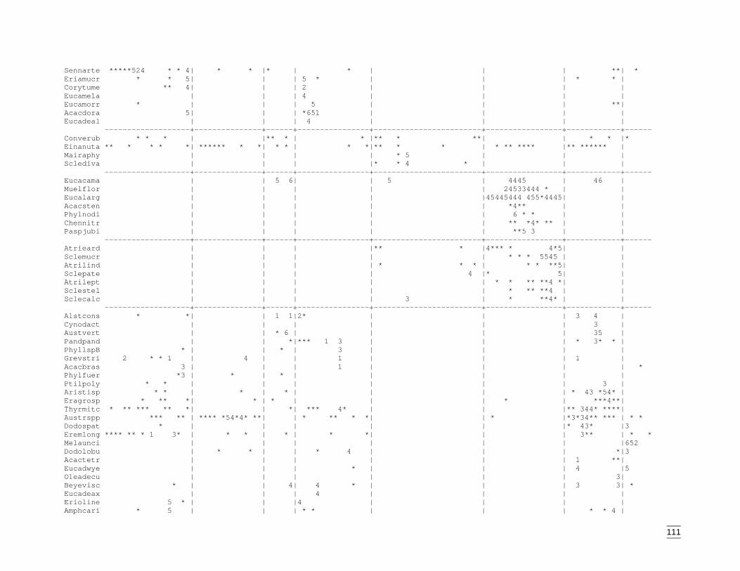
111
Sennarte *****524 * * 4| * * |* | * | | | **| * Eriamucr * * 5| | | 5 * | | | * * | Corytume ** 4| | | 2 | | | | Eucamela | | | 4 | | | | Eucamorr * | | | 5 | | | **| Acacdora 5| | | *651 | | | | Eucadeal | | | 4 | | | | -------------------+---------------+------+----------------+------------------------+-----------------+------------+------ Converub * * * | |** * | * |** * **| | * * |* Einanuta ** * * * *| ****** * *| * * | * *|** * * | * ** **** |** ****** | Mairaphy | | | | * 5 | | | Sclediva | | | |* * 4 * | | | -------------------+---------------+------+----------------+------------------------+-----------------+------------+------ Eucacama | | 5 6| | 5 | 4445 | 46 | Muelflor | | | | | 24533444 * | | Eucalarg | | | | |45445444 455*4445| | Acacsten | | | | | *4** | | Phylnodi | | | | | 6 * * | | Chennitr | | | | | ** *4* ** | | Paspjubi | | | | | **5 3 | | -------------------+---------------+------+----------------+------------------------+-----------------+------------+------ Atrieard | | | |** * |4*** * 4*5| | Sclemucr | | | | | * * * 5545 | | Atrilind | | | | * * * | * * **5| | Sclepate | | | | 4 |* 5| | Atrilept | | | | | * * ** **4 *| | Sclestel | | | | | * ** **4 | | Sclecalc | | | | 3 | * **4* | | -------------------+---------------+------+----------------+------------------------+-----------------+------------+------ Alstcons * *| | 1 1|2* | | | 3 4 | Cynodact | | | | | | 3 | Austvert | | * 6 | | | | 35 | Pandpand | | *|*** 1 3 | | | * 3* * | PhyllspB * | | * | 3 | | | | Grevstri 2 * * 1 | 4 | | 1 | | | 1 | Acacbras 3 | | | 1 | | | | * Phylfuer *3 | * | * | | | | | Ptilpoly * * | | | | | | 3 | Aristisp * * | * | * | | | | * 43 *54* | Eragrosp * ** *| * | * | | | * | ***4**| Thyrmitc * ** *** ** *| | *| *** 4* | | |** 344* ****| Austrspp *** ** | **** *54*4* **| | * ** * *| | * |*3*34** *** | * * Dodospat * | | | | | |* 43* |3 Eremlong **** ** * 1 3* | * * | * | * *| | | 3** | * * Melaunci | | | | | | |652 Dodolobu | * * | | * 4 | | | *|3 Acactetr | | | | | | 1 **| Eucadwye | | | * | | | 4 |5 Oleadecu | | | | | | 3| Beyevisc * | | 4| 4 * | | | 3 3| * Eucadeax | | | 4 | | | | Erioline 5 * | | |4 | | | | Amphcari * 5 | | | * * | | | * * 4 |
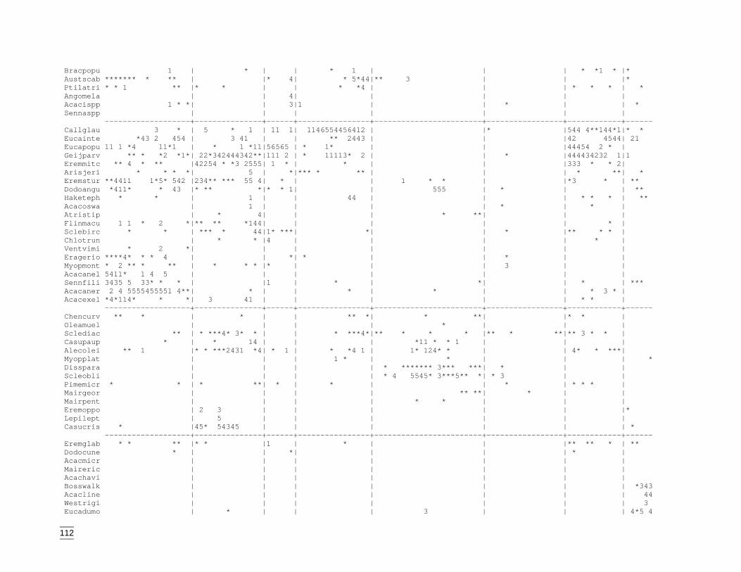
112
Bracpopu 1 | * | | * 1 | | | * *1 * |* Austscab ******* * ** | |* 4| * 5*44|** 3 | | |* Ptilatri * * 1 ** |* * | | * *4 | | | * * * | * Angomela | | 4| | | | | Acacispp 1 * *| | 3|1 | | * | | * Sennaspp | | | | | | | -------------------+---------------+------+----------------+------------------------+-----------------+------------+------ Callglau 3 * | 5 * 1 | 11 1| 1146554456412 | |* |544 4**144*1|* * Eucainte *43 2 454 | 3 41 | | ** 2443 | | |42 4544| 21 Eucapopu 11 1 *4 11*1 | * 1 *11|56565 | * 1* | | |44454 2 * | Geijparv ** * *2 *1*| 22*342444342**|111 2 | * 11113* 2 | | * |444434232 1|1 Eremmitc ** 4 * ** |42254 * *3 2555| 1 * | * | | |333 * * 2| Arisjeri * * * *| 5 | *|*** * ** | | | * **| * Eremstur **4411 1*5* 542 |234** *** 55 4| * | | 1 * * | |*3 * | ** Dodoangu *411* * 43 |* ** *|* * 1| | 555 | * | | ** Haketeph * * | 1 | | 44 | | | * * * | ** Acacoswa | 1 | | | | * | * | Atristip | * 4| | | * **| | | Flinmacu 1 1 * 2 *|** ** *144| | | | | * | Sclebirc * * | *** * 44|1* ***| *| | * |** * * | Chlotrun | * * |4 | | | | * | Ventvimi * 2 *| | | | | | | Eragerio ****4* * * 4 | | *| * | | * | | Myopmont * 2 ** * ** | * * * |* | | | 3 | | Acacanel 5411* 1 4 5 | | | | | | | Sennfili 3435 5 33* * * | |1 | * | *| | * | *** Acacaner 2 4 5555455551 4**| * | | * | * | | * 3 * | Acacexel *4*114* * *| 3 41 | | | | | * * | -------------------+---------------+------+----------------+------------------------+-----------------+------------+------ Chencurv ** * | * | | ** *| * **| |* * | Oleamuel | | | | * | | | Sclediac ** | * ***4* 3* * | | * ***4*|** * * * |** * **|** 3 * * | Casupaup * | * 14 | | | *11 * * 1 | | | Alecolei ** 1 |* * ***2431 *4| * 1 | * *4 1 | 1* 124* * | | 4* * ***| Myopplat | | | 1 * | * | | | * Disspara | | | | * ******* 3*** ***| * | | Scleobli | | | | * 4 5545* 3***5** *| * 3 | | Pimemicr * * | * **| * | * | | * | * * * | Mairgeor | | | | ** **| * | | Mairpent | | | | * * | | | Eremoppo | 2 3 | | | | | |* Lepilept | 5 | | | | | | Casucris * |45* 54345 | | | | | | * -------------------+---------------+------+----------------+------------------------+-----------------+------------+------ Eremglab * * ** |* * |1 | * | | |** ** * | ** Dodocune * | | *| | | | * | Acacmicr | | | | | | | Maireric | | | | | | | Acachavi | | | | | | | Bosswalk | | | | | | | *343 Acacline | | | | | | | 44 Westrigi | | | | | | | 3 Eucadumo | * | | | 3 | | | 4*5 4
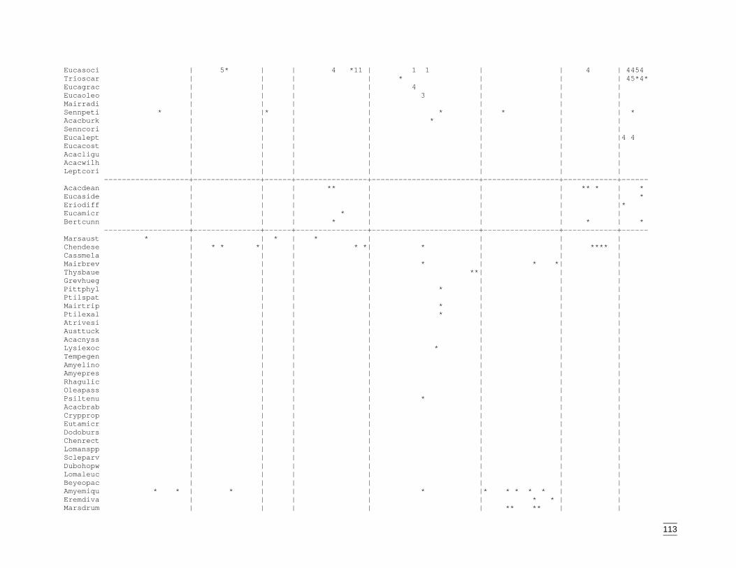
113
Eucasoci | 5* | | 4 *11 | 1 1 | | 4 | 4454 Trioscar | | | | * | | | 45*4* Eucagrac | | | | 4 | | | Eucaoleo | | | | 3 | | | Mairradi | | | | | | | Sennpeti * | |* | | * | * | | * Acacburk | | | | * | | | Senncori | | | | | | | Eucalept | | | | | | |4 4 Eucacost | | | | | | | Acacligu | | | | | | | Acacwilh | | | | | | | Leptcori | | | | | | | -------------------+---------------+------+----------------+------------------------+-----------------+------------+------ Acacdean | | | ** | | | ** * | * Eucaside | | | | | | | * Eriodiff | | | | | | |* Eucamicr | | | * | | | | Bertcunn | | | * | | | * | * -------------------+---------------+------+----------------+------------------------+-----------------+------------+------ Marsaust * | | * | * | | | | Chendese | * * *| | * *| * | | **** | Cassmela | | | | | | | Mairbrev | | | | * | * *| | Thysbaue | | | | **| | | Grevhueg | | | | | | | Pittphyl | | | | * | | | Ptilspat | | | | | | | Mairtrip | | | | * | | | Ptilexal | | | | * | | | Atrivesi | | | | | | | Austtuck | | | | | | | Acacnyss | | | | | | | Lysiexoc | | | | * | | | Tempegen | | | | | | | Amyelino | | | | | | | Amyepres | | | | | | | Rhagulic | | | | | | | Oleapass | | | | | | | Psiltenu | | | | * | | | Acacbrab | | | | | | | Crypprop | | | | | | | Eutamicr | | | | | | | Dodoburs | | | | | | | Chenrect | | | | | | | Lomanspp | | | | | | | Scleparv | | | | | | | Dubohopw | | | | | | | Lomaleuc | | | | | | | Beyeopac | | | | | | | Amyemiqu * * | * | | | * |* * * * * | | Eremdiva | | | | | * * | | Marsdrum | | | | | ** ** | |
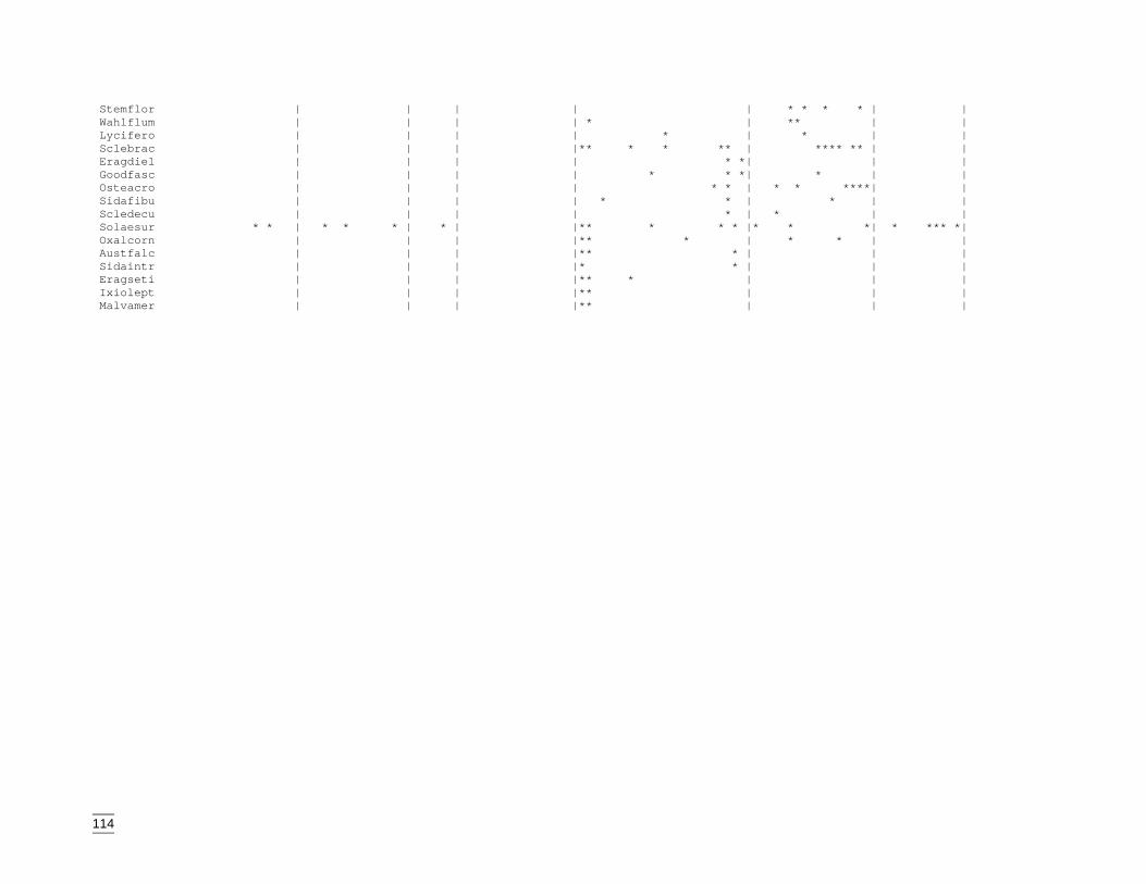
114
Stemflor | | | | | * * * * | | Wahlflum | | | | * | ** | | Lycifero | | | | * | * | | Sclebrac | | | |** * * ** | **** ** | | Eragdiel | | | | * *| | | Goodfasc | | | | * * *| * | | Osteacro | | | | * * | * * ****| | Sidafibu | | | | * * | * | | Scledecu | | | | * | * | | Solaesur * * | * * * | * | |** * * * |* * *| * *** *| Oxalcorn | | | |** * | * * | | Austfalc | | | |** * | | | Sidaintr | | | |* * | | | Eragseti | | | |** * | | | Ixiolept | | | |** | | | Malvamer | | | |** | | |
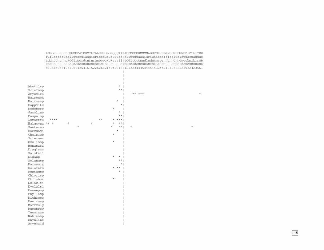
115
AMBBPPBPBBPLMMMMPATBHMTLTALRRRBLBLQQQTT|ABBMCCCHMMMMABBTMHPHLWMBBMBBMWBBLPTLTTBR rliuooooouoaiiuuoruiaauiuriooouauauuuoo|riiuuuuaaaiuriuaaaoaielooiuoleuuaouauuuo uddnoonpnnpkddllpurdtnrnrunbbbckckaaall|uddlttttnndludnnntotnndnndnndncckprkrrcb 000000000000000000000000000000000000000|0000000000000000000000000000000000000000 513565355165165643641615226265214646812|1213234445444544324521246532323532423561 | | | | Abutilsp * | Sclerosp **| Amyemira | ** *** * Mairench | Maireasp * | Cappmitc *| Dodoboro * | Jasmline * | Paspalsp **| Lomaeffu **** ** * ***| Halgcyna ** * * * * **| Santacum * * **| * * Boerdomi * | Cheisieb * | Scleconv | Oxalissp * | Monapara | Eraglacu | Salskali | Sidasp * * | Solanusp **| Parseuca *| Solafero * ** | Rostadsc * | Chlorisp | Ptilobov * | Solaclei | Evolalsi | Enneapsp | Phyllasp | Dichrepe | Panicusp | Marrvulg | Rumebrow | Teucrace | Wahlensp | Rhynline | Amyemaid |
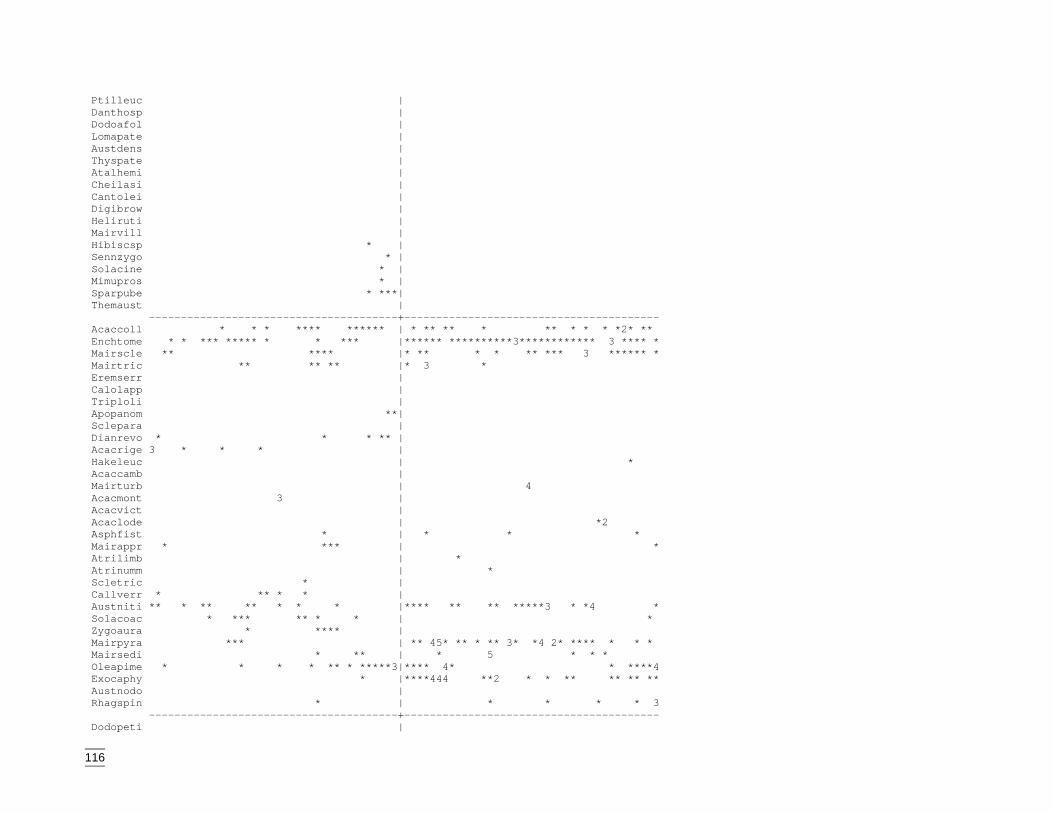
116
Ptilleuc | Danthosp | Dodoafol | Lomapate | Austdens | Thyspate | Atalhemi | Cheilasi | Cantolei | Digibrow | Heliruti | Mairvill | Hibiscsp * | Sennzygo * | Solacine * | Mimupros * | Sparpube * ***| Themaust | ---------------------------------------+---------------------------------------- Acaccoll * * * **** ****** | * ** ** * ** * * * *2* ** Enchtome * * *** ***** * * *** |****** **********3************ 3 **** * Mairscle ** **** |* ** * * ** *** 3 ****** * Mairtric ** ** ** |* 3 * Eremserr | Calolapp | Triploli | Apopanom **| Sclepara | Dianrevo * * * ** | Acacrige 3 * * * | Hakeleuc | * Acaccamb | Mairturb | 4 Acacmont 3 | Acacvict | Acaclode | *2 Asphfist * | * * * Mairappr * *** | * Atrilimb | * Atrinumm | * Scletric * | Callverr * ** * * | Austniti ** * ** ** * * * |**** ** ** *****3 * *4 * Solacoac * *** ** * * | * Zygoaura * **** | Mairpyra *** | ** 45* ** * ** 3* *4 2* **** * * * Mairsedi * ** | * 5 * * * Oleapime * * * * ** * *****3|**** 4* * ****4 Exocaphy * |****444 **2 * * ** ** ** ** Austnodo | Rhagspin * | * * * * 3 ---------------------------------------+---------------------------------------- Dodopeti |
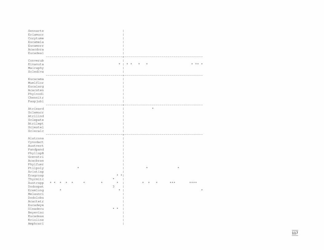
117
Sennarte | Eriamucr | Corytume | Eucamela | Eucamorr | Acacdora | Eucadeal | ---------------------------------------+---------------------------------------- Converub | Einanuta * | * * * * * ** * Mairaphy | Sclediva | ---------------------------------------+---------------------------------------- Eucacama | Muelflor | Eucalarg | Acacsten | Phylnodi | Chennitr | Paspjubi | ---------------------------------------+---------------------------------------- Atrieard | * Sclemucr | Atrilind | Sclepate | Atrilept | Sclestel | Sclecalc | ---------------------------------------+---------------------------------------- Alstcons | Cynodact | Austvert | Pandpand | PhyllspB | Grevstri | Acacbras | Phylfuer | Ptilpoly * | * * Aristisp | Eragrosp * *| Thyrmitc * | Austrspp * * * * * * * * | * * * *** **** Dodospat 3 | Eremlong * * | * Melaunci | Dodolobu | Acactetr | Eucadwye | Oleadecu * * | Beyevisc | Eucadeax | Erioline | Amphcari |
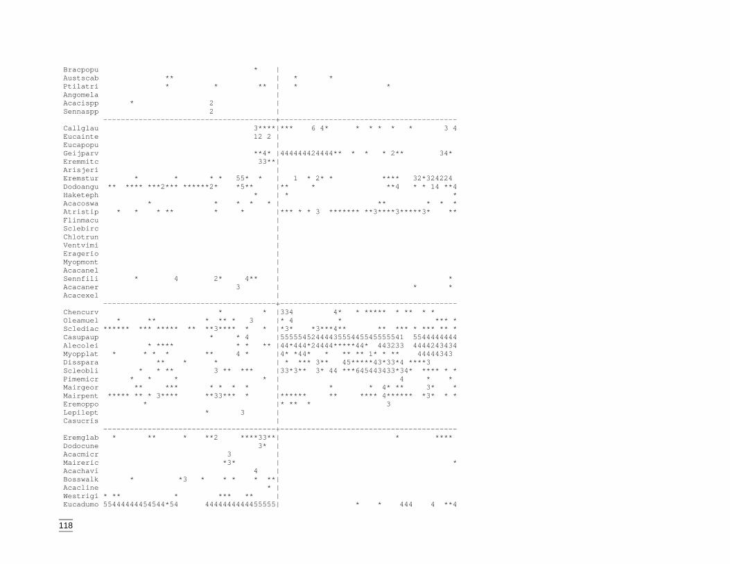
118
Bracpopu * | Austscab ** | * * Ptilatri * * ** | * * Angomela | Acacispp * 2 | Sennaspp 2 | ---------------------------------------+---------------------------------------- Callglau 3****|*** 6 4* * * * * * 3 4 Eucainte 12 2 | Eucapopu | Geijparv **4* |444444424444** * * * 2** 34* Eremmitc 33**| Arisjeri | Eremstur * * * * 55* * | 1 * 2* * **** 32*324224 Dodoangu ** **** ***2*** ******2* *5** |** * **4 * * 14 **4 Haketeph * | * * Acacoswa * * * * * | ** * * * Atristip * * * ** * * |*** * * 3 ******* **3****3*****3* ** Flinmacu | Sclebirc | Chlotrun | Ventvimi | Eragerio | Myopmont | Acacanel | Sennfili * 4 2* 4** | * Acacaner 3 | * * Acacexel | ---------------------------------------+---------------------------------------- Chencurv * * |334 4* * ***** * ** * * Oleamuel * ** * ** * 3 |* 4 * *** * Sclediac ****** *** ***** ** **3**** * * |*3* *3***4** ** *** * *** ** * Casupaup * * 4 |5555545244443555445545555541 5544444444 Alecolei * **** * * ** |44*444*24444*****44* 443233 4444243434 Myopplat * * * * ** 4 * |4* *44* * ** ** 1* * ** 44444343 Disspara ** * * | * *** 3** 45*****43*33*4 ****3 Scleobli * * ** 3 ** *** |33*3** 3* 44 ***645443433*34* **** * * Pimemicr * * * * | 4 * * Mairgeor ** *** * * * * | * * 4* ** 3* * Mairpent ***** ** * 3**** **33*** * |****** ** **** 4****** *3* * * Eremoppo * |* ** * 3 Lepilept * 3 | Casucris | ---------------------------------------+---------------------------------------- Eremglab * ** * **2 ****33**| * **** Dodocune 3* | Acacmicr 3 | Maireric *3* | * Acachavi 4 | Bosswalk * *3 * * * * **| Acacline * | Westrigi * ** * *** ** | Eucadumo 55444444454544*54 4444444444455555| * * 444 4 **4
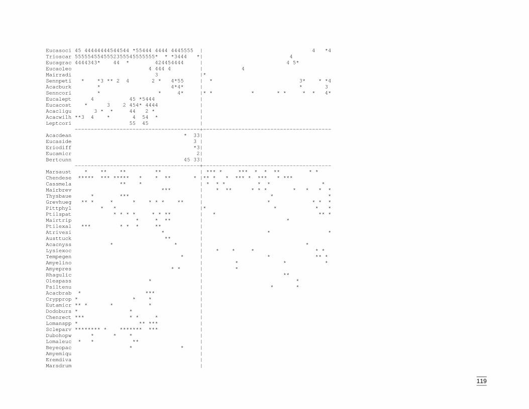
119
Eucasoci 45 44444444544544 *55444 4444 4445555 | 4 *4 Trioscar 5555545545552355545555555* * *3444 *| 4 Eucagrac 4444343* 44 * 424454444 | 4 5* Eucaoleo 4 444 4 | 4 Mairradi 3 |* Sennpeti * *3 ** 2 4 2 * 4*55 | * 3* * *4 Acacburk * 4*4* | * 3 Senncori * * 4* |* * * * * * * 4* Eucalept 4 45 *5444 | Eucacost * 3 2 454* 4444 | Acacligu 3 * * 44 2 * | Acacwilh **3 4 * 4 54 * | Leptcori 55 45 | ---------------------------------------+---------------------------------------- Acacdean * 33| Eucaside 3 | Eriodiff *3| Eucamicr 2| Bertcunn 45 33| ---------------------------------------+---------------------------------------- Marsaust * ** ** ** | *** * *** * * ** * * Chendese ***** *** ***** * * ** * |** * * *** * *** * *** Cassmela ** * | * * * * * * Mairbrev *** | * ** * * * * * * * Thysbaue * *** | * * Grevhueg ** * * * * * * ** | * * * * Pittphyl * * |* * * * Ptilspat * * * * * * ** | * ** * Mairtrip * * ** | * Ptilexal *** * * * ** | Atrivesi * | * * Austtuck ** | Acacnyss * * | * Lysiexoc | * * * * * Tempegen * | * ** * Amyelino | * * * Amyepres * * | * Rhagulic | ** Oleapass * | * Psiltenu | * * Acacbrab * *** | Crypprop * * * | Eutamicr ** * * * | Dodoburs * * | Chenrect *** * * * | Lomanspp * ** *** | Scleparv ******** * ******* *** | Dubohopw * * * | Lomaleuc * * ** | Beyeopac * * | Amyemiqu | Eremdiva | Marsdrum |
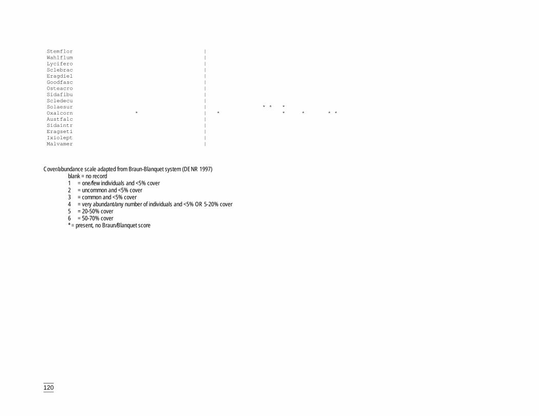
120
Stemflor | Wahlflum | Lycifero | Sclebrac | Eragdiel | Goodfasc | Osteacro | Sidafibu | Scledecu | Solaesur | * * * Oxalcorn * | * * * * * Austfalc | Sidaintr | Eragseti | Ixiolept | Malvamer |
Cover/abundance scale adapted from Braun-Blanquet system (DENR 1997)blank = no record1 = one/few individuals and <5% cover2 = uncommon and <5% cover3 = common and <5% cover4 = very abundant/any number of individuals and <5% OR 5-20% cover5 = 20-50% cover6 = 50-70% cover* = present, no Braun/Blanquet score
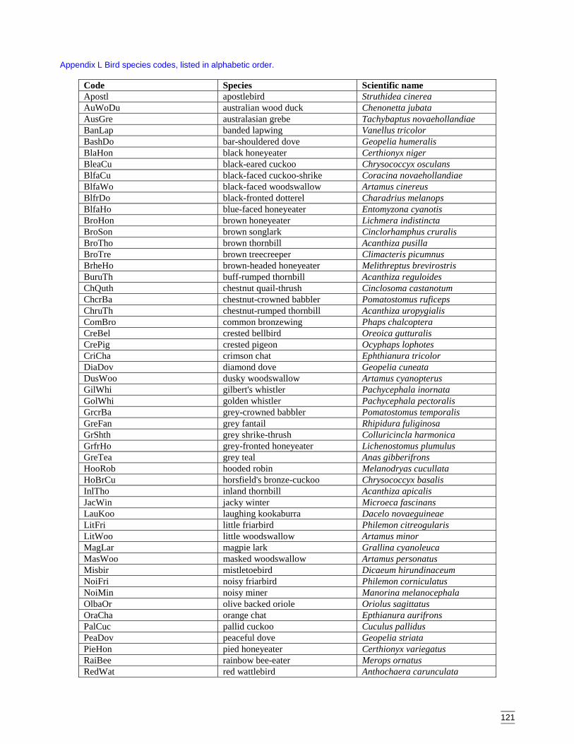
121
Appendix L Bird species codes, listed in alphabetic order.
Code Species Scientific nameApostl apostlebird Struthidea cinereaAuWoDu australian wood duck Chenonetta jubataAusGre australasian grebe Tachybaptus novaehollandiaeBanLap banded lapwing Vanellus tricolorBashDo bar-shouldered dove Geopelia humeralisBlaHon black honeyeater Certhionyx nigerBleaCu black-eared cuckoo Chrysococcyx osculansBlfaCu black-faced cuckoo-shrike Coracina novaehollandiaeBlfaWo black-faced woodswallow Artamus cinereusBlfrDo black-fronted dotterel Charadrius melanopsBlfaHo blue-faced honeyeater Entomyzona cyanotisBroHon brown honeyeater Lichmera indistinctaBroSon brown songlark Cinclorhamphus cruralisBroTho brown thornbill Acanthiza pusillaBroTre brown treecreeper Climacteris picumnusBrheHo brown-headed honeyeater Melithreptus brevirostrisBuruTh buff-rumped thornbill Acanthiza reguloidesChQuth chestnut quail-thrush Cinclosoma castanotumChcrBa chestnut-crowned babbler Pomatostomus ruficepsChruTh chestnut-rumped thornbill Acanthiza uropygialisComBro common bronzewing Phaps chalcopteraCreBel crested bellbird Oreoica gutturalisCrePig crested pigeon Ocyphaps lophotesCriCha crimson chat Ephthianura tricolorDiaDov diamond dove Geopelia cuneataDusWoo dusky woodswallow Artamus cyanopterusGilWhi gilbert's whistler Pachycephala inornataGolWhi golden whistler Pachycephala pectoralisGrcrBa grey-crowned babbler Pomatostomus temporalisGreFan grey fantail Rhipidura fuliginosaGrShth grey shrike-thrush Colluricincla harmonicaGrfrHo grey-fronted honeyeater Lichenostomus plumulusGreTea grey teal Anas gibberifronsHooRob hooded robin Melanodryas cucullataHoBrCu horsfield's bronze-cuckoo Chrysococcyx basalisInlTho inland thornbill Acanthiza apicalisJacWin jacky winter Microeca fascinansLauKoo laughing kookaburra Dacelo novaeguineaeLitFri little friarbird Philemon citreogularisLitWoo little woodswallow Artamus minorMagLar magpie lark Grallina cyanoleucaMasWoo masked woodswallow Artamus personatusMisbir mistletoebird Dicaeum hirundinaceumNoiFri noisy friarbird Philemon corniculatusNoiMin noisy miner Manorina melanocephalaOlbaOr olive backed oriole Oriolus sagittatusOraCha orange chat Epthianura aurifronsPalCuc pallid cuckoo Cuculus pallidusPeaDov peaceful dove Geopelia striataPieHon pied honeyeater Certhionyx variegatusRaiBee rainbow bee-eater Merops ornatusRedWat red wattlebird Anthochaera carunculata
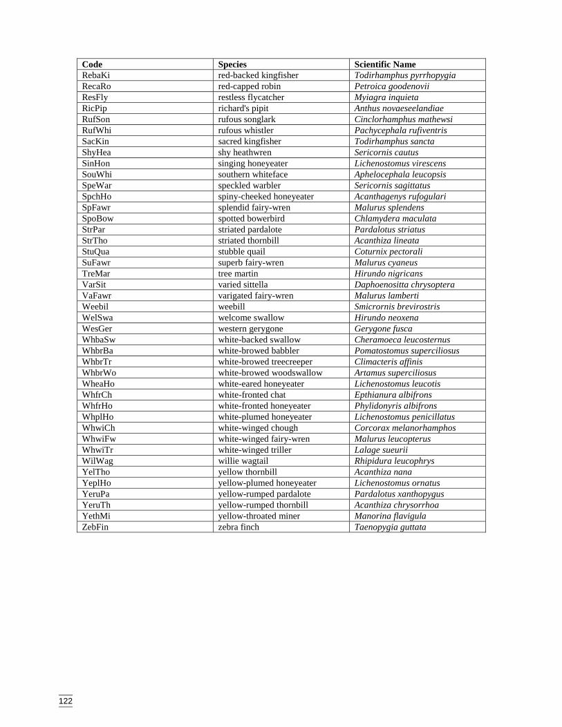
122
Code Species Scientific NameRebaKi red-backed kingfisher Todirhamphus pyrrhopygiaRecaRo red-capped robin Petroica goodenoviiResFly restless flycatcher Myiagra inquietaRicPip richard's pipit Anthus novaeseelandiaeRufSon rufous songlark Cinclorhamphus mathewsiRufWhi rufous whistler Pachycephala rufiventrisSacKin sacred kingfisher Todirhamphus sanctaShyHea shy heathwren Sericornis cautusSinHon singing honeyeater Lichenostomus virescensSouWhi southern whiteface Aphelocephala leucopsisSpeWar speckled warbler Sericornis sagittatusSpchHo spiny-cheeked honeyeater Acanthagenys rufogulariSpFawr splendid fairy-wren Malurus splendensSpoBow spotted bowerbird Chlamydera maculataStrPar striated pardalote Pardalotus striatusStrTho striated thornbill Acanthiza lineataStuQua stubble quail Coturnix pectoraliSuFawr superb fairy-wren Malurus cyaneusTreMar tree martin Hirundo nigricansVarSit varied sittella Daphoenositta chrysopteraVaFawr varigated fairy-wren Malurus lambertiWeebil weebill Smicrornis brevirostrisWelSwa welcome swallow Hirundo neoxenaWesGer western gerygone Gerygone fuscaWhbaSw white-backed swallow Cheramoeca leucosternusWhbrBa white-browed babbler Pomatostomus superciliosusWhbrTr white-browed treecreeper Climacteris affinisWhbrWo white-browed woodswallow Artamus superciliosusWheaHo white-eared honeyeater Lichenostomus leucotisWhfrCh white-fronted chat Epthianura albifronsWhfrHo white-fronted honeyeater Phylidonyris albifronsWhplHo white-plumed honeyeater Lichenostomus penicillatusWhwiCh white-winged chough Corcorax melanorhamphosWhwiFw white-winged fairy-wren Malurus leucopterusWhwiTr white-winged triller Lalage sueuriiWilWag willie wagtail Rhipidura leucophrysYelTho yellow thornbill Acanthiza nanaYeplHo yellow-plumed honeyeater Lichenostomus ornatusYeruPa yellow-rumped pardalote Pardalotus xanthopygusYeruTh yellow-rumped thornbill Acanthiza chrysorrhoaYethMi yellow-throated miner Manorina flavigulaZebFin zebra finch Taenopygia guttata
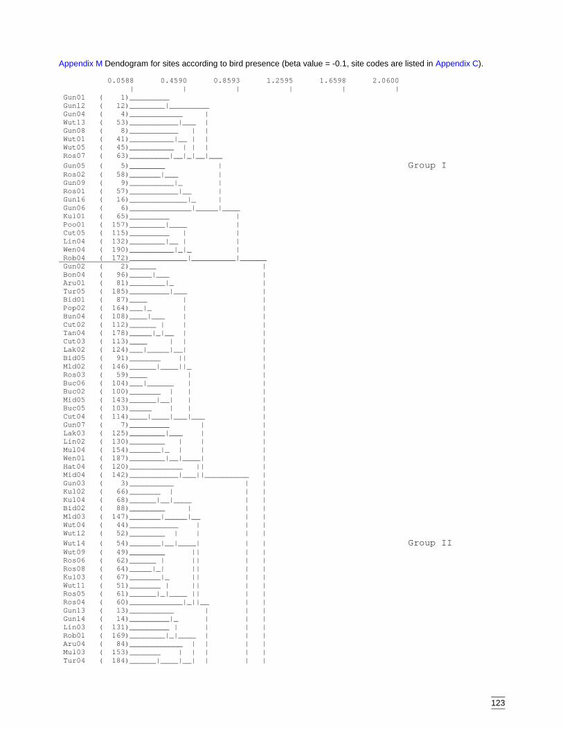
123
Appendix M Dendogram for sites according to bird presence (beta value = -0.1, site codes are listed in Appendix C).
0.0588 0.4590 0.8593 1.2595 1.6598 2.0600 | | | | | | Gun01 ( 1)_________ Gun12 ( 12)________|_________ Gun04 ( 4)____________ | Wut13 ( 53)___________|___ | Gun08 ( 8)___________ | | Wut01 ( 41)__________|__ | | Wut05 ( 45)__________ | | | Ros07 ( 63)_________|__|_|__|___ Gun05 ( 5)________ | Group I Ros02 ( 58)_______|___ | Gun09 ( 9)__________|_ | Ros01 ( 57)___________|__ | Gun16 ( 16)_____________|_ | Gun06 ( 6)______________|_____|____ Kul01 ( 65)_________ | Poo01 ( 157)________|____ | Cut05 ( 115)_________ | | Lin04 ( 132)________|__ | | Wen04 ( 190)__________|_|_ | Rob04 ( 172)_____________|__________|______ Gun02 ( 2)______ | Bon04 ( 96)_____|___ | Aru01 ( 81)________|_ | Tur05 ( 185)_________|___ | Bid01 ( 87)____ | | Pop02 ( 164)___|_ | | Bun04 ( 108)____|___ | | Cut02 ( 112)______ | | | Tan04 ( 178)_____|_|__ | | Cut03 ( 113)____ | | | Lak02 ( 124)___|_____|__| | Bid05 ( 91)_______ || | Mld02 ( 146)______|____||_ | Ros03 ( 59)____ | | Buc06 ( 104)___|______ | | Buc02 ( 100)_______ | | | Mid05 ( 143)______|__| | | Buc05 ( 103)_____ | | | Cut04 ( 114)____|____|___|___ | Gun07 ( 7)_________ | | Lak03 ( 125)________|___ | | Lin02 ( 130)________ | | | Mul04 ( 154)_______|_ | | | Wen01 ( 187)________|__|____| | Hat04 ( 120)____________ || | Mid04 ( 142)___________|___||__________ | Gun03 ( 3)__________ | | Kul02 ( 66)_______ | | | Kul04 ( 68)______|__|____ | | Bid02 ( 88)________ | | | Mld03 ( 147)_______|_____|__ | | Wut04 ( 44)___________ | | | Wut12 ( 52)________ | | | | Wut14 ( 54)_______|__|____| | | Group II Wut09 ( 49)________ || | | Ros06 ( 62)______ | || | | Ros08 ( 64)_____|_| || | | Kul03 ( 67)_______|_ || | | Wut11 ( 51)_______ | || | | Ros05 ( 61)______|_|____ || | | Ros04 ( 60)____________|_||__ | | Gun13 ( 13)__________ | | | Gun14 ( 14)_________|_ | | | Lin03 ( 131)_________ | | | | Rob01 ( 169)________|_|____ | | | Aru04 ( 84)____________ | | | | Mul03 ( 153)_______ | | | | | Tur04 ( 184)______|____|__| | | |
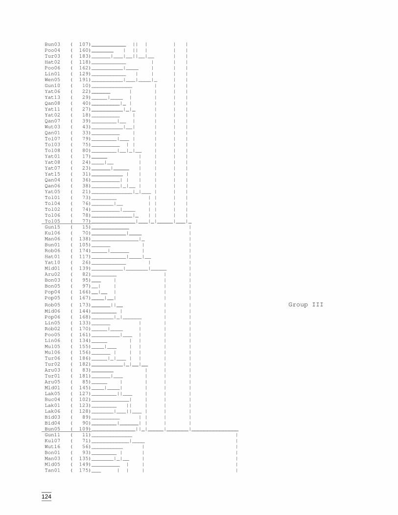
124
Bun03 ( 107)___________ || | | | Poo04 ( 160)_______ | || | | | Tur03 ( 183)______|___|__||__|__ | | Hat02 ( 118)___________ | | | Poo06 ( 162)__________|____ | | | Lin01 ( 129)___________ | | | | Wen05 ( 191)__________|___|____|_ | | Gun10 ( 10)_____________ | | | Yat06 ( 22)______ | | | | Yat13 ( 29)_____|____ | | | | Qan08 ( 40)_________|_ | | | | Yat11 ( 27)__________|_|_ | | | Yat02 ( 18)_________ | | | | Qan07 ( 39)________|__ | | | | Wut03 ( 43)__________|__| | | | Qan01 ( 33)_________ | | | | Tol07 ( 79)________|___ | | | | Tol03 ( 75)_________ | | | | | Tol08 ( 80)________|__|_|__ | | | Yat01 ( 17)_____ | | | | Yat08 ( 24)____|__ | | | | Yat07 ( 23)______|_____ | | | | Yat15 ( 31)__________ | | | | | Qan04 ( 36)_________| | | | | | Qan06 ( 38)_________|_|__ | | | | Yat05 ( 21)_____________|_|___ | | | Tol01 ( 73)________ | | | | Tol04 ( 76)_______|__ | | | | Tol02 ( 74)_________|____ | | | | Tol06 ( 78)_____________|_ | | | | Tol05 ( 77)______________|___|_|_____|___|_ Gun15 ( 15)____________ | Kul06 ( 70)___________|____ | Man06 ( 138)_______________|_ | Bun01 ( 105)______ | | Rob06 ( 174)_____|______ | | Hat01 ( 117)___________|____|__ | Yat10 ( 26)___________ | | Mid01 ( 139)__________|_______|_____ | Aru02 ( 82)________ | | Bon03 ( 95)___ | | | Bon05 ( 97)__| | | | Pop04 ( 166)__|__ | | | Pop05 ( 167)____|__| | | Rob05 ( 173)______||__ | | Group III Mid06 ( 144)________ | | | Pop06 ( 168)_______|_|______ | | Lin05 ( 133)______ | | | Rob02 ( 170)_____|____ | | | Poo05 ( 161)_________|___ | | | Lin06 ( 134)_____ | | | | Mul05 ( 155)____|___ | | | | Mul06 ( 156)______ | | | | | Tur06 ( 186)_____|_|___ | | | | Tur02 ( 182)__________|_|__|__ | | Aru03 ( 83)_______ | | | Tur01 ( 181)______|___ | | | Aru05 ( 85)_____ | | | | Mld01 ( 145)____|____| | | | Lak05 ( 127)________||___ | | | Buc04 ( 102)____________| | | | Lak01 ( 123)________ || | | | Lak06 ( 128)_______|___||___ | | | Bid03 ( 89)_________ | | | | Bid04 ( 90)________|______| | | | Bun05 ( 109)______________||_|_____|_______|_______________ Gun11 ( 11)_____________ | Kul07 ( 71)____________|____ | Wut16 ( 56)__________ | | Bon01 ( 93)________ | | | Man03 ( 135)_______|_|__ | | Mld05 ( 149)_________ | | | Tan01 ( 175)___ | | | |

125
Tan03 ( 177)__|_____|__|____|__ | Aru06 ( 86)____________ | | Pop03 ( 165)___________|______|_ | Kul08 ( 72)_________________ | | Man04 ( 136)____________ | | | Man05 ( 137)________ | | | | Mid03 ( 141)_______|___|____|__|_ | Bid06 ( 92)__________ | | Hat05 ( 121)_________|_____ | | Bun06 ( 110)___________ | | | Cut06 ( 116)__________|___| | | Rob03 ( 171)_____________||__ | | Bon02 ( 94)________ | | | Poo02 ( 158)_______|____ | | | Wen02 ( 188)___________|_ | | | Group IV Poo03 ( 159)________ | | | | Tan06 ( 180)_______|____|___|___|______ | Yat03 ( 19)________ | | Yat09 ( 25)_______|_______ | | Yat04 ( 20)______ | | | Qan05 ( 37)_____|_ | | | Qan03 ( 35)______|_______|__ | | Yat12 ( 28)_____ | | | Yat14 ( 30)____|___ | | | Qan02 ( 34)_______|_____ | | | Wut02 ( 42)_ | | | | Wut07 ( 47)|________ | | | | Wut06 ( 46)_____ | | | | | Wut10 ( 50)____|___|__ | | | | Wut08 ( 48)_______ | | | | | Wut15 ( 55)______|___|_|___|_________|__ | Kul05 ( 69)_____________ | | Bun02 ( 106)____________|_______ | | Mid02 ( 140)___________________|________|_________________|______________ Yat16 ( 32)____________________ | Tan02 ( 176)___________________|________ | Bon06 ( 98)________________ | | Wen06 ( 192)_______________|________ | | Group V Buc01 ( 99)_____________ | | | Buc03 ( 101)____________|___ | | | Cut01 ( 111)_________ | | | | Tan05 ( 179)________|______|_______|___|_______ | Hat03 ( 119)____________ | | Mul02 ( 152)___________|_____ | | Mul01 ( 151)________ | | | Wen03 ( 189)_______|________|___ | | Pop01 ( 163)___________________|_ | | Group VI Hat06 ( 122)_________ | | | Mld06 ( 150)________|__ | | | Mld04 ( 148)__________|___ | | | Lak04 ( 126)_____________|______|_____________|_________________________| | | | | | | 0.0588 0.4590 0.8593 1.2595 1.6598 2.0600
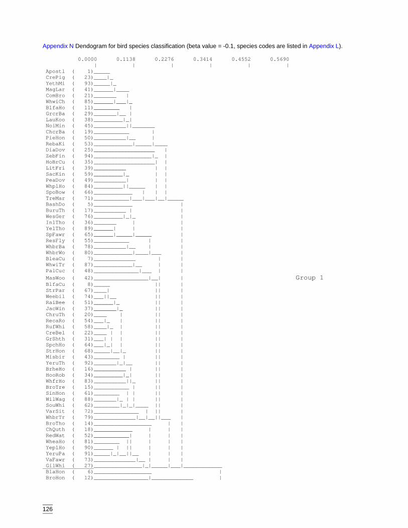
126
Appendix N Dendogram for bird species classification (beta value = -0.1, species codes are listed in Appendix L).
0.0000 0.1138 0.2276 0.3414 0.4552 0.5690 | | | | | | Apostl ( 1)_____ CrePig ( 23)____|_ YethMi ( 93)_____|_ MagLar ( 41)______|____ ComBro ( 21)_______ | WhwiCh ( 85)______|___|_ BlfaHo ( 11)________ | GrcrBa ( 29)_______|__ | LauKoo ( 38)_________|_| NoiMin ( 45)__________||_______ ChcrBa ( 19)___________ | PieHon ( 50)__________|__ | RebaKi ( 53)____________|_____|____ DiaDov ( 25)___________________ | ZebFin ( 94)__________________|_ | HoBrCu ( 35)___________________| | LitFri ( 39)__________ | | SacKin ( 59)_________|_ | | PeaDov ( 49)__________| | | WhplHo ( 84)_________||_____ | | SpoBow ( 66)____________ | | | TreMar ( 71)___________|___|___|__|_____ BashDo ( 5)____________ | BuruTh ( 17)__________ | | WesGer ( 76)_________|_|_ | InlTho ( 36)_______ | | YelTho ( 89)______| | | SpFawr ( 65)______|_____|_____ | ResFly ( 55)___________ | | WhbrBa ( 78)__________|__ | | WhbrWo ( 80)____________|____|___ | BleaCu ( 7)_____________ | | WhwiTr ( 87)____________|__ | | PalCuc ( 48)______________|___ | | MasWoo ( 42)_________________|__| | Group 1 BlfaCu ( 8)_____ || | StrPar ( 67)____| || | Weebil ( 74)___||__ || | RaiBee ( 51)______|_ || | JacWin ( 37)_______|_ || | ChruTh ( 20)____ | || | RecaRo ( 54)___|_ | || | RufWhi ( 58)____|_ | || | CreBel ( 22)____ | | || | GrShth ( 31)___| | | || | SpchHo ( 64)___|_| | || | StrHon ( 68)_____|__|_ || | Misbir ( 43)________ | || | YeruTh ( 92)_______|_|__ || | BrheHo ( 16)__________ | || | HooRob ( 34)_________|_| || | WhfrHo ( 83)__________||_ || | BroTre ( 15)___________ | || | SinHon ( 61)________ | | || | WilWag ( 88)_______|_ | | || | SouWhi ( 62)________|_|_|____ || | VarSit ( 72)______________ | || | WhbrTr ( 79)_____________|__|__||___ | BroTho ( 14)__________________ | | ChQuth ( 18)____________ | | | RedWat ( 52)___________| | | | WheaHo ( 81)________ || | | | YeplHo ( 90)______ | || | | | YeruPa ( 91)_____|_|__||__ | | | VaFawr ( 73)_____________|__ | | | GilWhi ( 27)_______________|_|_____|___|____________ BlaHon ( 6)__________________ | BroHon ( 12)_________________|_____________ |
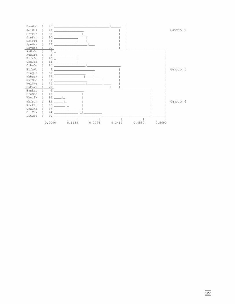
127
DusWoo ( 26)______________________________|_____ | GolWhi ( 28)________________ | | Group 2 GrfrHo ( 32)_______________|__ | | GreFan ( 30)_____________ | | | NoiFri ( 44)____________|____|_ | | SpeWar ( 63)__________________|___ | | ShyHea ( 60)_____________________|_____________|___|_____________________ AuWoDu ( 2)_ | AusGre ( 3)|____________ | BlfrDo ( 10)_ | | GreTea ( 33)|___________|_____ | OlbaOr ( 46)_________________|__________________ | BlfaWo ( 9)______________________ | | Group 3 StuQua ( 69)_________________ | | | WhbaSw ( 77)________________|____|_____ | | RufSon ( 57)__________________ | | | WelSwa ( 75)_________________|________|____ | | SuFawr ( 70)______________________________|____|_________________ | BanLap ( 4)________________ | | BroSon ( 13)_____ | | | WhwiFw ( 86)____|_ | | | WhfrCh ( 82)_____|_ | | | Group 4 RicPip ( 56)______|_ | | | OraCha ( 47)_______|______ | | | CriCha ( 24)_____________|_|__________ | | LitWoo ( 40)_________________________|__________________________|_______| | | | | | | 0.0000 0.1138 0.2276 0.3414 0.4552 0.5690
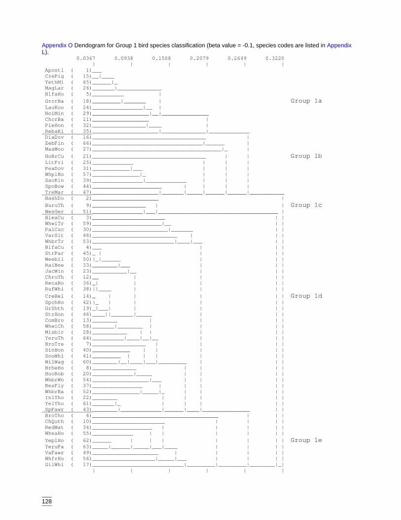
128
Appendix O Dendogram for Group 1 bird species classification (beta value = -0.1, species codes are listed in AppendixL). 0.0367 0.0938 0.1508 0.2079 0.2649 0.3220 | | | | | | Apostl ( 1)___ CrePig ( 15)__|____ YethMi ( 65)______|_ MagLar ( 26)_______|______________ BlfaHo ( 5)__________ | GrcrBa ( 18)_________|_______ | Group 1a LauKoo ( 24)________________|__ | NoiMin ( 29)__________________|__|_______________ ChcrBa ( 11)__________________ | PieHon ( 32)_________________|____ | RebaKi ( 35)_____________________|______________|_____________ DiaDov ( 16)____________________________________ | ZebFin ( 66)___________________________________|______ | MasWoo ( 27)_________________________________________|_ | HoBrCu ( 21)____________________________________ | | Group 1b LitFri ( 25)_____________ | | | PeaDov ( 31)____________|___ | | | WhplHo ( 57)_______________|_ | | | SacKin ( 39)________________|_____________ | | | SpoBow ( 44)______________________ | | | | TreMar ( 47)_____________________|_______|_____|______|______|___________ BashDo ( 2)_____________________ | BuruTh ( 9)_________________ | | Group 1c WesGer ( 51)________________|___|______________________________________ | BleaCu ( 3)_______________________ | | WhwiTr ( 59)______________________|__ | | PalCuc ( 30)________________________|_______ | | VarSit ( 48)___________________________ | | | WhbrTr ( 53)__________________________|____|___ | | BlfaCu ( 4)___ | | | StrPar ( 45)_ | | | | Weebil ( 50)|_|______ | | | RaiBee ( 33)________|___ | | | JacWin ( 23)___________|__ | | | ChruTh ( 12)__ | | | | RecaRo ( 36)_| | | | | RufWhi ( 38)||____ | | | | CreBel ( 14)_ | | | | | Group 1d SpchHo ( 42)|_ | | | | | GrShth ( 19)_|___| | | | | StrHon ( 46)____||_______|_____ | | | ComBro ( 13)________ | | | | WhwiCh ( 58)_______|________ | | | | Misbir ( 28)___________ | | | | | YeruTh ( 64)__________|____|__|__ | | | BroTre ( 7)_________________ | | | | SinHon ( 40)____________ | | | | | SouWhi ( 41)_________ | | | | | | WilWag ( 60)________|__|____|___|_________ | | | BrheHo ( 8)______________ | | | | HooRob ( 20)_____________|_____ | | | | WhbrWo ( 54)__________________|___ | | | | ResFly ( 37)________________ | | | | | WhbrBa ( 52)_______________|_____|_ | | | | InlTho ( 22)________ | | | | | YelTho ( 61)_______|_ | | | | | SpFawr ( 43)________|_____________|______|____|_______________ | | BroTho ( 6)________________________________________ | | | ChQuth ( 10)_______________________ | | | | RedWat ( 34)___________________ | | | | | WheaHo ( 55)_____________ | | | | | | YeplHo ( 62)______ | | | | | | | Group 1e YeruPa ( 63)_____|______|_____|___|____ | | | | VaFawr ( 49)_____________________ | | | | | WhfrHo ( 56)____________________|_____|___ | | | | GilWhi ( 17)_____________________________|_________|_________|________|_| | | | | | |
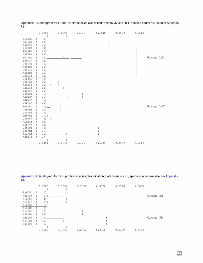
129
Appendix P Dendogram for Group 1d bird species classification (beta value = -0.1, species codes are listed in AppendixL).
0.0355 0.0786 0.1217 0.1648 0.2079 0.2510 | | | | | | BleaCu ( 1)________________________________________ PalCuc ( 13)_______________________________ | WhwiTr ( 30)______________________________|________|_________________ BrheHo ( 4)_____________________________ | InlTho ( 10)_______________ | | SpFawr ( 21)___________ | | | YelTho ( 32)__________|___|_______ | | Group 1d1 YeruTh ( 33)_____________________|______|_______ | HooRob ( 9)_________________________ | | WhbrWo ( 28)________________________|_____ | | ResFly ( 16)________________________ | | | WhbrBa ( 26)_______________________|_____|_____|____ | VarSit ( 24)_______________________________________|________________|____ BlfaCu ( 2)________ | StrPar ( 22)___ | | Weebil ( 25)__|____|___ | RaiBee ( 14)__________|______ | JacWin ( 11)________________|______ | ComBro ( 6)______________ | | WhwiCh ( 29)_____________|________|______ | ChruTh ( 5)_______ | | StrHon ( 23)______|__ | | RecaRo ( 15)__ | | | Group 1d2 RufWhi ( 17)_|______|___ | | CreBel ( 7)_ | | | SpchHo ( 20)|__ | | | GrShth ( 8)__|________|___ | | Misbir ( 12)______________|____ | | SinHon ( 18)__________________|_________|____ | BroTre ( 3)______________________ | | SouWhi ( 19)_____________ | | | WilWag ( 31)____________|________|__________|________________ | WhbrTr ( 27)________________________________________________|___________| | | | | | | 0.0355 0.0786 0.1217 0.1648 0.2079 0.2510
Appendix Q Dendogram for Group 3 bird species classification (beta value = -0.1, species codes are listed in AppendixL).
0.0000 0.1330 0.2660 0.3990 0.5320 0.6650 | | | | | | AuWoDu ( 1)_ AusGre ( 2)|____________ Group 3a BlfrDo ( 4)_ | GreTea ( 5)|___________|_______ OlbaOr ( 6)___________________|_________________________________________ BlfaWo ( 3)_______________________ | StuQua ( 8)______________________| | WhbaSw ( 11)______________________|_______________ | RufSon ( 7)___________ | | Group 3b WelSwa ( 10)__________|___________________ | | SuFawr ( 9)_____________________________|_______|______________________| | | | | | | 0.0000 0.1330 0.2660 0.3990 0.5320 0.6650
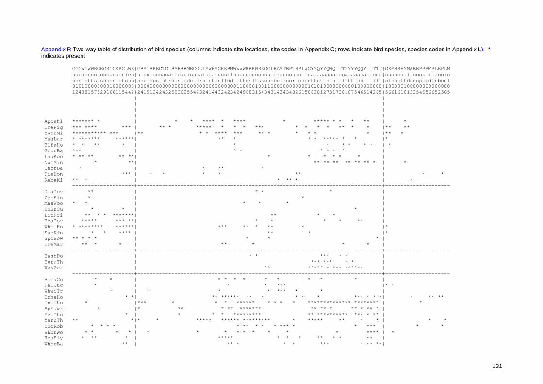
131
Appendix R Two-way table of distribution of bird species (columns indicate site locations, site codes in Appendix C; rows indicate bird species, species codes in Appendix L). *indicates present
GGGWGWWRGRGRGGKPCLWR|GBATBPBCTCLBMRBBMBCGLLMWHMGKKBMWWWWRRKWRRGGLRAMTBPTHPLWGYYQYYQWQTTTYYYYQQYTTTTT|GKMBRHYMABBPPRMPLRPLM uuuuuuuouououuuouieo|uoruiouuauailouuiuuuaiueaiuuuiluuuuoouuoouuioruuuouaoieuaaaaaauaoooaaaaaaaooooo|uuauoaairoooooioiooiu nnntnttsnsnsnnlotnnb|nnurdpntntkddsccdctnknlntdnllddttttssltssnnnbulrnortonnnttnttntnlllttttnntlllll|nlnnbttdunnppbdpnbonl 01010000000010000000|0000000000000000000000000000000011000010011000000000000101010000000000100000000|100000100000000000000 12438157529166115444|2415124243252362554732414432423424968315434314343432615063812731738187546514265|566161012354556652565 | | | | | | | | Apostl ******* * | * * **** * **** * ***** * * * ** | * CrePig *** **** *** | ** * ***** * * * *** * * * * ** * * |** ** YethMi *********** *** |** * * **** *** ** * * * * * |** * MagLar * ******* ******| ** * * * ***** * * |* BlfaHo * * ** * | * * * * * * | * GrcrBa *** | * * * * * * | LauKoo * ** ** ** **| * * * * * * | NoiMin * **| ** ** ** ** ** ** * | * ChcrBa * | * ** * | PieHon *** | * * * * ** | * * RebaKi ** * | * ** * | * --------------------+-------------------------------------------------------------------------------+--------------------- DiaDov ** | * * * | ZebFin * | * | MasWoo * * | * * * | HoBrCu * * | * | LitFri ** * * *******| ** * * | PeaDov ***** *** **| * * * * ** | WhplHo * ******** ******| *** ** * ** * |* SacKin * * **** | ** * |* SpoBow ** * * * | * * * | TreMar ** * * | ** * * * | --------------------+-------------------------------------------------------------------------------+--------------------- BashDo | * * *** * * | BuruTh | *** *** * * | WesGer | ** ***** * *** ****** | --------------------+-------------------------------------------------------------------------------+--------------------- BleaCu * * | * * * * * * * * * | PalCuc * | * * *** |* * WhwiTr * | * * * *** * * | BrheHo * *| ** ****** ** * * * * *** * * *| * ** ** InlTho * |*** * * * ****** * * * * ************** ******** | * SpFawr * |* ** * ** ******* ** ** * ** * ** * | YelTho * | * * * ********* ** ********** *** * ** | YeruTh ** *|* * ***** ****** ********* * ***** ** * * | * * HooRob * * * * | * ** * * * *** * * *** | * * WhbrWo * * * * | * * * * * * * * * **** | * ResFly * ** * | ***** * * * ** * * ** | WhbrBa ** | ** * * * *** * ** **|
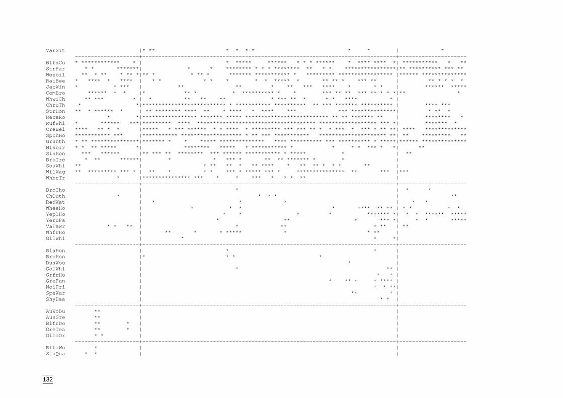
132
VarSit |* ** * * * * * * | * --------------------+-------------------------------------------------------------------------------+--------------------- BlfaCu * ************ * | * ***** ****** * * * ****** * **** **** *| *********** * ** StrPar * * *******| * * ******** * * * ******** ** * * ****************|** ********** *** ** Weebil ** * ** * ** *|** * * ** * ******* *********** * ********* ***************** |****** ************** RaiBee * **** * **** | * * * * * * * ***** * ** ** * *** ** | ** * * * * JacWin * * *** | ** ** * ** *** **** * * * | ****** ***** ComBro ****** * * |* ** * * ********** * * *** ** ** *** ** * * *|** * WhwiCh ** *** * | * ** ** ** * *** ** * * * **** * | ChruTh * *|************************** * *********** ********** ** *** ******* ********** | **** *** StrHon ** * ****** * | ** ******** **** ** * **** * **** *** *** **************| * ** * RecaRo * *|***************** ******* ***** ************************** ** ** ******* ** | ******** * RufWhi * ****** ***|********* **** ************************************* ****************** *** *| ******* * CreBel **** ** * * |***** * *** ****** * * **** * ********* *** *** ** * * *** * *** * ** **| **** ************* SpchHo *********** *** |*********** ******************* * ** *** *********** ********************* **| ** ********* ** GrShth * ** ***************|******* * * ***** ************** **** ********** *** ********** * *****|****** ************** Misbir * * ** ***** *| ******** ***** * *********** * * * * *** * *| ** SinHon *** ****** |** *** ** ******** *** ****** *********** * ***** * | ** BroTre * ** ******| * * *** * ** ** ******* * * | SouWhi ** | * ** ** * ** **** * ** ** * * * ** | WilWag ** ********* *** * | ** * * * *** * ***** *** * *************** ** *** |*** WhbrTr * |*************** *** * * *** * * * ** | --------------------+-------------------------------------------------------------------------------+--------------------- BroTho | * | * * ChQuth * | * * * | ** RedWat | * * * | * * WheaHo | * * * * **** ** ** | * * * * YeplHo | * * * * ******* *| * * ****** ***** YeruPa | * ** * *** *| * * ***** VaFawr * * ** | * ** * ** | ** WhfrHo | ** * * ***** * * ** | GilWhi | * * *| --------------------+-------------------------------------------------------------------------------+--------------------- BlaHon | * * | BroHon |* * * * | DusWoo | * | GolWhi | * ** | GrfrHo | * * | GreFan | * ** * * **** | NoiFri | * * **| SpeWar | ** * | ShyHea | * * | --------------------+-------------------------------------------------------------------------------+--------------------- AuWoDu ** | | AusGre ** | | BlfrDo ** * | | GreTea ** * | | OlbaOr * * | | --------------------+-------------------------------------------------------------------------------+--------------------- BlfaWo * | | StuQua * * | |
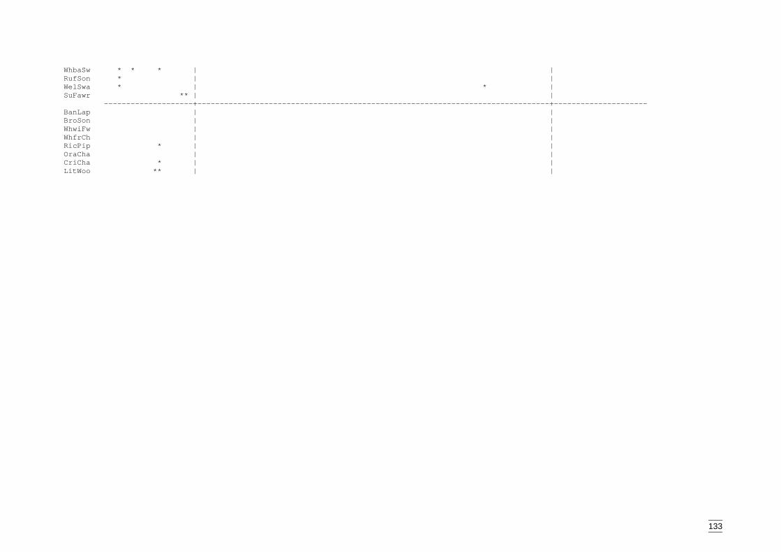
133
WhbaSw * * * | | RufSon * | | WelSwa * | * | SuFawr ** | | --------------------+-------------------------------------------------------------------------------+--------------------- BanLap | | BroSon | | WhwiFw | | WhfrCh | | RicPip * | | OraCha | | CriCha * | | LitWoo ** | |
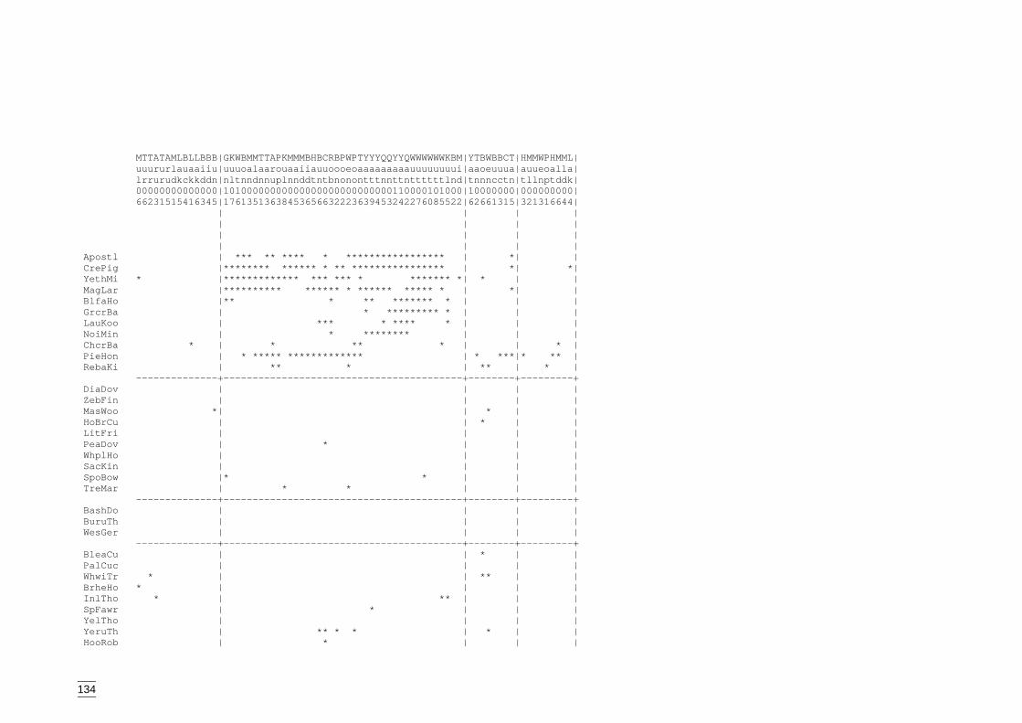
134
MTTATAMLBLLBBB|GKWBMMTTAPKMMMBHBCRBPWPTYYYQQYYQWWWWWWKBM|YTBWBBCT|HMMWPHMML| uuururlauaaiiu|uuuoalaarouaaiiauuoooeoaaaaaaaaauuuuuuuui|aaoeuuua|auueoalla| lrrurudkckkddn|nltnndnnuplnnddtntbnonontttnnttnttttttlnd|tnnncctn|tllnptddk| 00000000000000|10100000000000000000000000000110000101000|10000000|000000000| 66231515416345|17613513638453656632223639453242276085522|62661315|321316644| | | | | | | | | | | | | | | | | Apostl | *** ** **** * ***************** | *| | CrePig |******** ****** * ** **************** | *| *| YethMi * |************* *** *** * ******* *| * | | MagLar |********** ****** * ****** ***** * | *| | BlfaHo |** * ** ******* * | | | GrcrBa | * ********* * | | | LauKoo | *** * **** * | | | NoiMin | * ******** | | | ChcrBa * | * ** * | | * | PieHon | * ***** ************* | * ***|* ** | RebaKi | ** * | ** | * | --------------+-----------------------------------------+--------+---------+ DiaDov | | | | ZebFin | | | | MasWoo *| | * | | HoBrCu | | * | | LitFri | | | | PeaDov | * | | | WhplHo | | | | SacKin | | | | SpoBow |* * | | | TreMar | * * | | | --------------+-----------------------------------------+--------+---------+ BashDo | | | | BuruTh | | | | WesGer | | | | --------------+-----------------------------------------+--------+---------+ BleaCu | | * | | PalCuc | | | | WhwiTr * | | ** | | BrheHo * | | | | InlTho * | ** | | | SpFawr | * | | | YelTho | | | | YeruTh | ** * * | * | | HooRob | * | | |
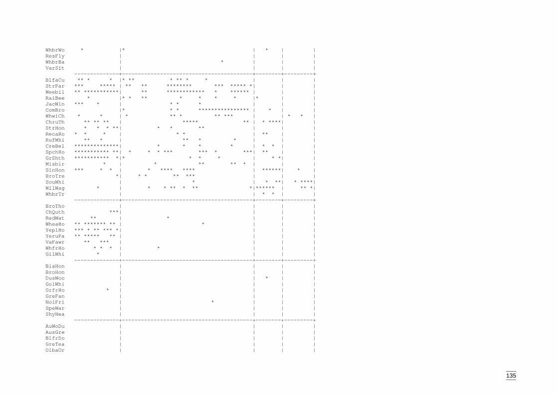
135
WhbrWo * |* | * | | ResFly | | | | WhbrBa | * | | | VarSit | | | | --------------+-----------------------------------------+--------+---------+ BlfaCu ** * * |* ** * ** * * | | | StrPar *** ***** | ** ** ******** *** ***** *| | | Weebil ** ***********| ** ************ * ****** | | | RaiBee * |* * ** * * * * |* | | JacWin *** * | * * * | | | ComBro |* * * **************** | * | | WhwiCh * * | * ** * ** *** | | * * | ChruTh ** ** ** | ***** ** | * ****| | StrHon * * * **| * * ** | | | RecaRo * * * | * * | ** | | RufWhi ** * | ** * * | | | CreBel **************| * * * * | * * | | SpchHo *********** **| * * * *** *** * ***| ** | | GrShth *********** *|* * * * | * *| | Misbir * | * ** ** * | | | SinHon *** * * | * **** **** | ******| * | BroTre *| * * ** *** | | | SouWhi | * | * **| * ****| WilWag * | * * ** * ** *|****** | ** *| WhbrTr | | * * | | --------------+-----------------------------------------+--------+---------+ BroTho | | | | ChQuth ***| | | | RedWat ** | * | | | WheaHo ** ******* ** | * | | | YeplHo *** * ** *** *| | | | YeruPa ** ***** ** | | | | VaFawr ** *** | | | | WhfrHo * * * | * | | | GilWhi * | | | | --------------+-----------------------------------------+--------+---------+ BlaHon | | | | BroHon | | | | DusWoo | | * | | GolWhi | | | | GrfrHo * | | | | GreFan | | | | NoiFri | * | | | SpeWar | | | | ShyHea | | | | --------------+-----------------------------------------+--------+---------+ AuWoDu | | | | AusGre | | | | BlfrDo | | | | GreTea | | | | OlbaOr | | | |
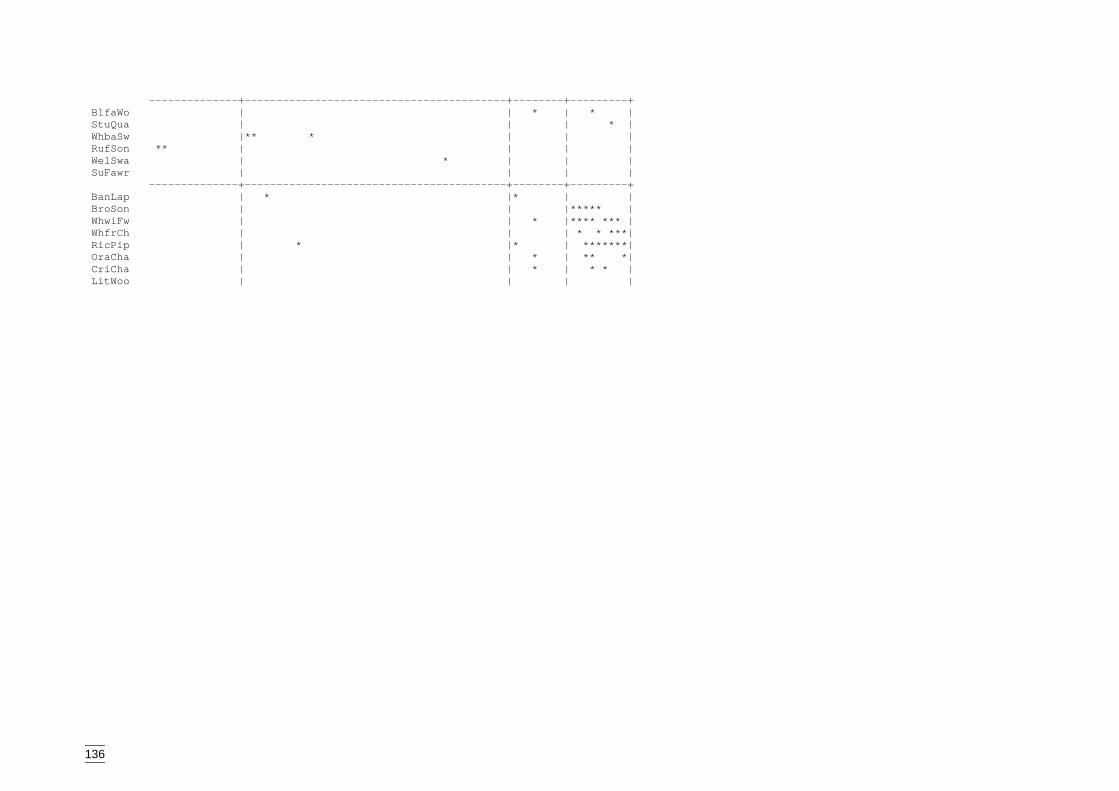
136
--------------+-----------------------------------------+--------+---------+ BlfaWo | | * | * | StuQua | | | * | WhbaSw |** * | | | RufSon ** | | | | WelSwa | * | | | SuFawr | | | | --------------+-----------------------------------------+--------+---------+ BanLap | * |* | | BroSon | | |***** | WhwiFw | | * |**** *** | WhfrCh | | | * * ***| RicPip | * |* | *******| OraCha | | * | ** *| CriCha | | * | * * | LitWoo | | | |
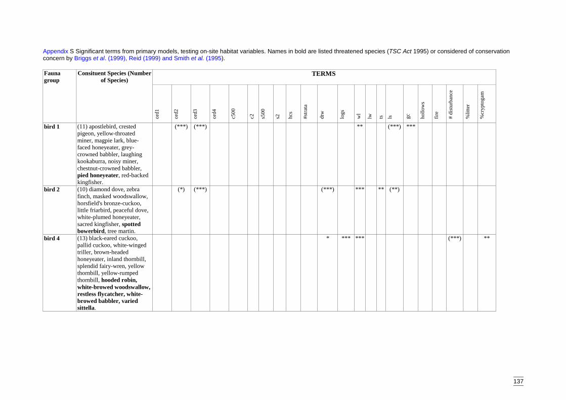
137
Appendix S Significant terms from primary models, testing on-site habitat variables. Names in bold are listed threatened species (TSC Act 1995) or considered of conservationconcern by Briggs et al. (1999), Reid (1999) and Smith et al. (1995).
TERMSFaunagroup
Consituent Species (Numberof Species)
ord1
ord2
ord3
ord4
c500
c2 s500
s2 hcs
#stra
ta
dtw
logs
wl
lw ts ls gc hollo
ws
fire
# di
stur
banc
e
%lit
ter
%cr
ypto
gam
bird 1 (11) apostlebird, crestedpigeon, yellow-throatedminer, magpie lark, blue-faced honeyeater, grey-crowned babbler, laughingkookaburra, noisy miner,chestnut-crowned babbler,pied honeyeater, red-backedkingfisher.
(***) (***) ** (***) ***
bird 2 (10) diamond dove, zebrafinch, masked woodswallow,horsfield's bronze-cuckoo,little friarbird, peaceful dove,white-plumed honeyeater,sacred kingfisher, spottedbowerbird, tree martin.
(*) (***) (***) *** ** (**)
bird 4 (13) black-eared cuckoo,pallid cuckoo, white-wingedtriller, brown-headedhoneyeater, inland thornbill,splendid fairy-wren, yellowthornbill, yellow-rumpedthornbill, hooded robin,white-browed woodswallow,restless flycatcher, white-browed babbler, variedsittella.
* *** *** (***) **
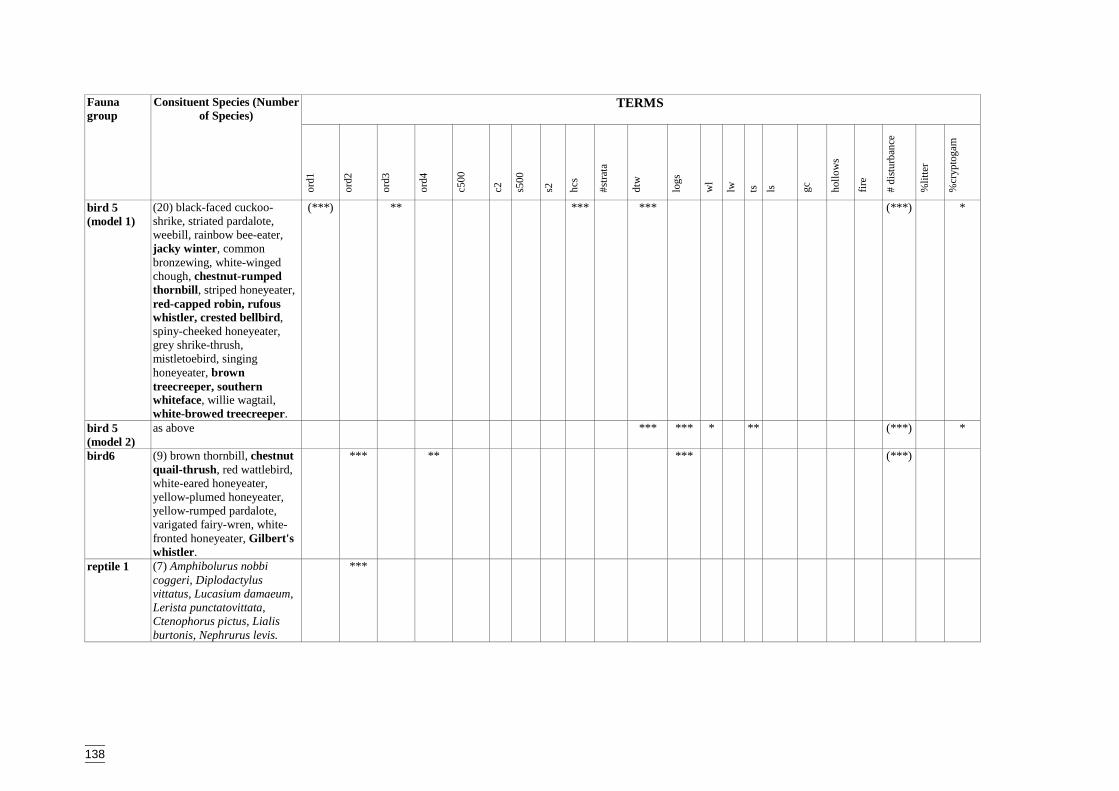
138
TERMSFaunagroup
Consituent Species (Numberof Species)
ord1
ord2
ord3
ord4
c500
c2 s500
s2 hcs
#stra
ta
dtw
logs
wl
lw ts ls gc hollo
ws
fire
# di
stur
banc
e
%lit
ter
%cr
ypto
gam
bird 5(model 1)
(20) black-faced cuckoo-shrike, striated pardalote,weebill, rainbow bee-eater,jacky winter, commonbronzewing, white-wingedchough, chestnut-rumpedthornbill, striped honeyeater,red-capped robin, rufouswhistler, crested bellbird,spiny-cheeked honeyeater,grey shrike-thrush,mistletoebird, singinghoneyeater, browntreecreeper, southernwhiteface, willie wagtail,white-browed treecreeper.
(***) ** *** *** (***) *
bird 5(model 2)
as above *** *** * ** (***) *
bird6 (9) brown thornbill, chestnutquail-thrush, red wattlebird,white-eared honeyeater,yellow-plumed honeyeater,yellow-rumped pardalote,varigated fairy-wren, white-fronted honeyeater, Gilbert'swhistler.
*** ** *** (***)
reptile 1 (7) Amphibolurus nobbicoggeri, Diplodactylusvittatus, Lucasium damaeum,Lerista punctatovittata,Ctenophorus pictus, Lialisburtonis, Nephrurus levis.
***

139
TERMSFaunagroup
Consituent Species (Numberof Species)
ord1
ord2
ord3
ord4
c500
c2 s500
s2 hcs
#stra
ta
dtw
logs
wl
lw ts ls gc hollo
ws
fire
# di
stur
banc
e
%lit
ter
%cr
ypto
gam
reptile3 (20) Cryptoblepharuscarnabyi, Gehyra variegata,Heteronotia binoei, Morethiaboulengeri, Lerista muelleri,Egernia striolata,Diplodactylus intermedius,Gehyra dubia, Oeduramarmorata, Pogona barbata,Ctenotus schomburgkii,Pygopus nigriceps,Diplodactylus steindachneri,Rhynchoedura ornata,Underwoodisaurus milii,Ctenophorus nuchalis,Ctenotus allotropis,Diplodactylus tessellatus,Menetia greyii, Pogonavitticeps.
(***) *** ** * (*)
reptile 5 (7) Ctenophorus fordi,Ctenotus atlas, Diplodactyluselderi, Delma australis,Egernia inornata, Morethiaobscura, Ctenotusbrachyonyx.
*** * *
bat 1 (9) Chalinolobus gouldii,Nyctophilus geoffroyi,Scotorepens greyii,Nyctophilus species,Vespadelus sp, Mormopterussp (big penis), Chalinolobuspicatus, Nyctophilustimoriensis, Vespadelusvulturnus.
*** *** (*) (***)
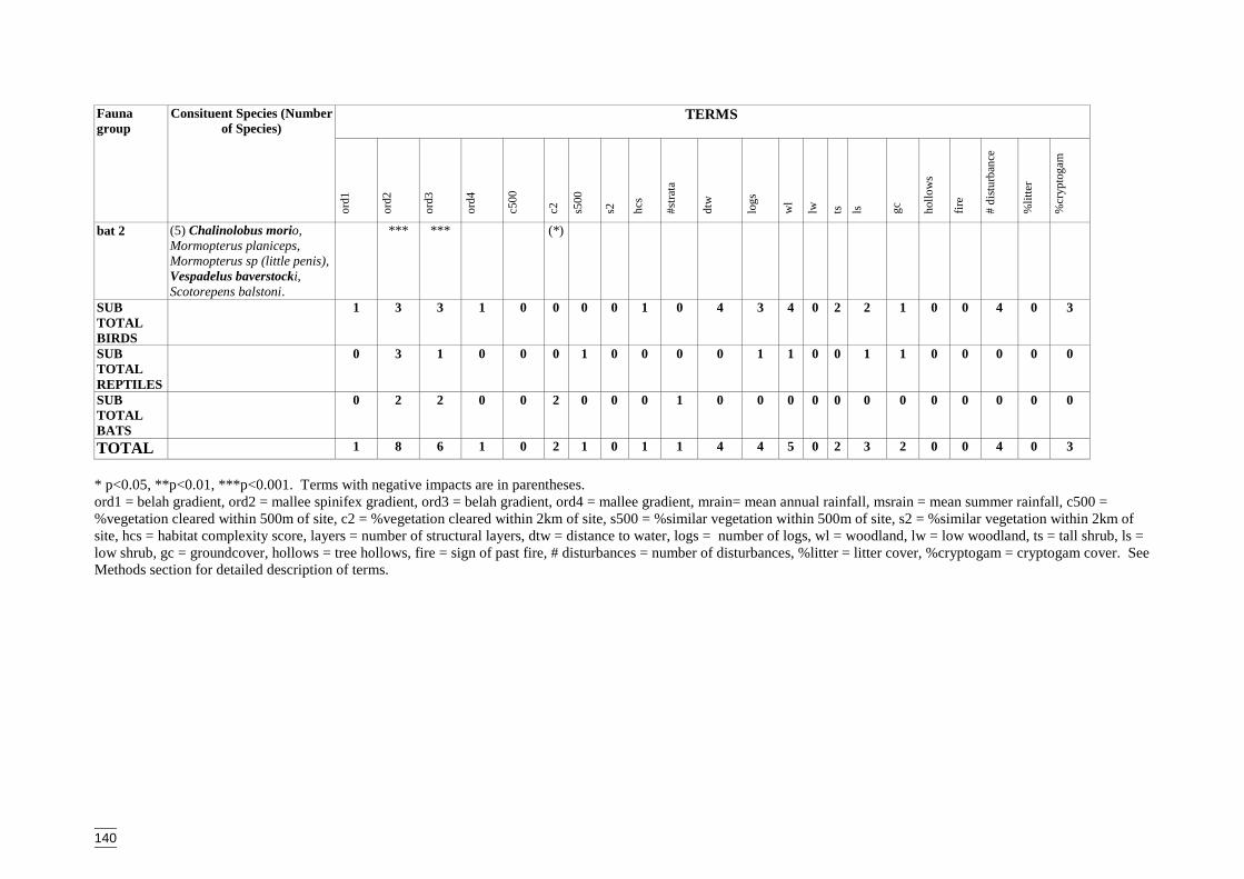
140
TERMSFaunagroup
Consituent Species (Numberof Species)
ord1
ord2
ord3
ord4
c500
c2 s500
s2 hcs
#stra
ta
dtw
logs
wl
lw ts ls gc hollo
ws
fire
# di
stur
banc
e
%lit
ter
%cr
ypto
gam
bat 2 (5) Chalinolobus morio,Mormopterus planiceps,Mormopterus sp (little penis),Vespadelus baverstocki,Scotorepens balstoni.
*** *** (*)
SUBTOTALBIRDS
1 3 3 1 0 0 0 0 1 0 4 3 4 0 2 2 1 0 0 4 0 3
SUBTOTALREPTILES
0 3 1 0 0 0 1 0 0 0 0 1 1 0 0 1 1 0 0 0 0 0
SUBTOTALBATS
0 2 2 0 0 2 0 0 0 1 0 0 0 0 0 0 0 0 0 0 0 0
TOTAL 1 8 6 1 0 2 1 0 1 1 4 4 5 0 2 3 2 0 0 4 0 3
* p<0.05, **p<0.01, ***p<0.001. Terms with negative impacts are in parentheses.ord1 = belah gradient, ord2 = mallee spinifex gradient, ord3 = belah gradient, ord4 = mallee gradient, mrain= mean annual rainfall, msrain = mean summer rainfall, c500 =%vegetation cleared within 500m of site, c2 = %vegetation cleared within 2km of site, s500 = %similar vegetation within 500m of site, s2 = %similar vegetation within 2km ofsite, hcs = habitat complexity score, layers = number of structural layers, dtw = distance to water, logs = number of logs, wl = woodland, lw = low woodland, ts = tall shrub, ls =low shrub, gc = groundcover, hollows = tree hollows, fire = sign of past fire, # disturbances = number of disturbances, %litter = litter cover, %cryptogam = cryptogam cover. SeeMethods section for detailed description of terms.
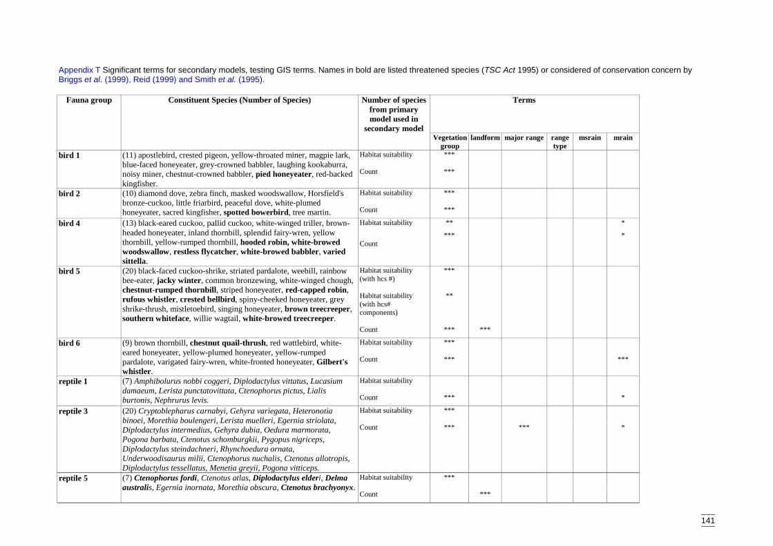
141
Appendix T Significant terms for secondary models, testing GIS terms. Names in bold are listed threatened species (TSC Act 1995) or considered of conservation concern byBriggs et al. (1999), Reid (1999) and Smith et al. (1995).
Fauna group Constituent Species (Number of Species) Number of speciesfrom primarymodel used in
secondary model
Terms
Vegetationgroup
landform major range rangetype
msrain mrain
bird 1 Habitat suitability ***(11) apostlebird, crested pigeon, yellow-throated miner, magpie lark,blue-faced honeyeater, grey-crowned babbler, laughing kookaburra,noisy miner, chestnut-crowned babbler, pied honeyeater, red-backedkingfisher.
Count ***
bird 2 Habitat suitability ***(10) diamond dove, zebra finch, masked woodswallow, Horsfield'sbronze-cuckoo, little friarbird, peaceful dove, white-plumedhoneyeater, sacred kingfisher, spotted bowerbird, tree martin. Count ***
bird 4 Habitat suitability ** *(13) black-eared cuckoo, pallid cuckoo, white-winged triller, brown-headed honeyeater, inland thornbill, splendid fairy-wren, yellowthornbill, yellow-rumped thornbill, hooded robin, white-browedwoodswallow, restless flycatcher, white-browed babbler, variedsittella.
Count*** *
bird 5 Habitat suitability(with hcs #)
***
Habitat suitability(with hcs#components)
**
(20) black-faced cuckoo-shrike, striated pardalote, weebill, rainbowbee-eater, jacky winter, common bronzewing, white-winged chough,chestnut-rumped thornbill, striped honeyeater, red-capped robin,rufous whistler, crested bellbird, spiny-cheeked honeyeater, greyshrike-thrush, mistletoebird, singing honeyeater, brown treecreeper,southern whiteface, willie wagtail, white-browed treecreeper.
Count *** ***
bird 6 Habitat suitability ***(9) brown thornbill, chestnut quail-thrush, red wattlebird, white-eared honeyeater, yellow-plumed honeyeater, yellow-rumpedpardalote, varigated fairy-wren, white-fronted honeyeater, Gilbert'swhistler.
Count *** ***
reptile 1 Habitat suitability(7) Amphibolurus nobbi coggeri, Diplodactylus vittatus, Lucasiumdamaeum, Lerista punctatovittata, Ctenophorus pictus, Lialisburtonis, Nephrurus levis. Count *** *
reptile 3 Habitat suitability ***(20) Cryptoblepharus carnabyi, Gehyra variegata, Heteronotiabinoei, Morethia boulengeri, Lerista muelleri, Egernia striolata,Diplodactylus intermedius, Gehyra dubia, Oedura marmorata,Pogona barbata, Ctenotus schomburgkii, Pygopus nigriceps,Diplodactylus steindachneri, Rhynchoedura ornata,Underwoodisaurus milii, Ctenophorus nuchalis, Ctenotus allotropis,Diplodactylus tessellatus, Menetia greyii, Pogona vitticeps.
Count *** *** *
reptile 5 Habitat suitability ***(7) Ctenophorus fordi, Ctenotus atlas, Diplodactylus elderi, Delmaaustralis, Egernia inornata, Morethia obscura, Ctenotus brachyonyx.
Count ***
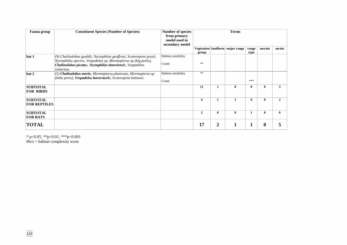
142
Fauna group Constituent Species (Number of Species) Number of speciesfrom primarymodel used in
secondary model
Terms
Vegetationgroup
landform major range rangetype
msrain mrain
bat 1 Habitat suitability(9) Chalinolobus gouldii, Nyctophilus geoffroyi, Scotorepens greyii,Nyctophilus species, Vespadelus sp, Mormopterus sp (big penis),Chalinolobus picatus, Nyctophilus timoriensis, Vespadelusvulturnus.
Count **
bat 2 Habitat suitability **(5) Chalinolobus morio, Mormopterus planiceps, Mormopterus sp(little penis), Vespadelus baverstocki, Scotorepens balstoni.
Count ***
SUBTOTALFOR BIRDS
11 1 0 0 0 3
SUBTOTALFOR REPTILES
4 1 1 0 0 2
SUBTOTALFOR BATS
2 0 0 1 0 0
TOTAL 17 2 1 1 0 5
* p<0.05, **p<0.01, ***p<0.001#hcs = habitat complexity score

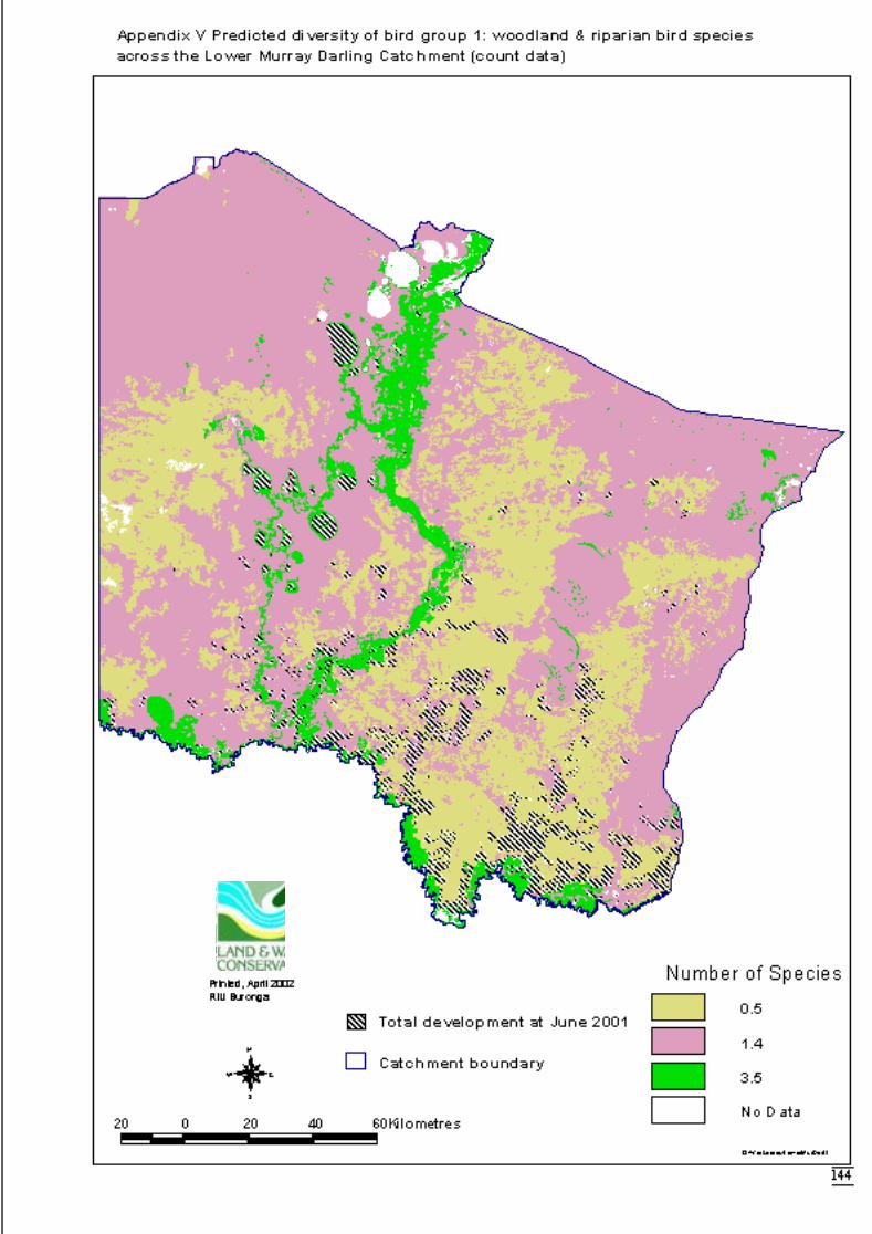

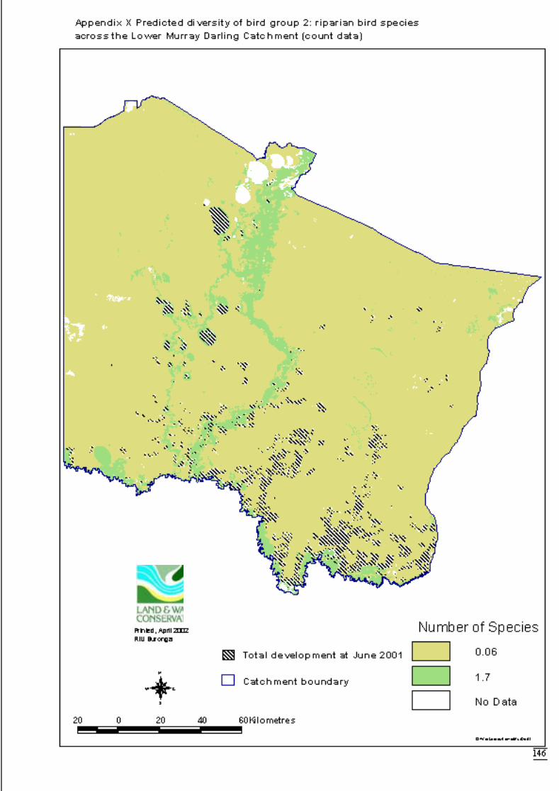

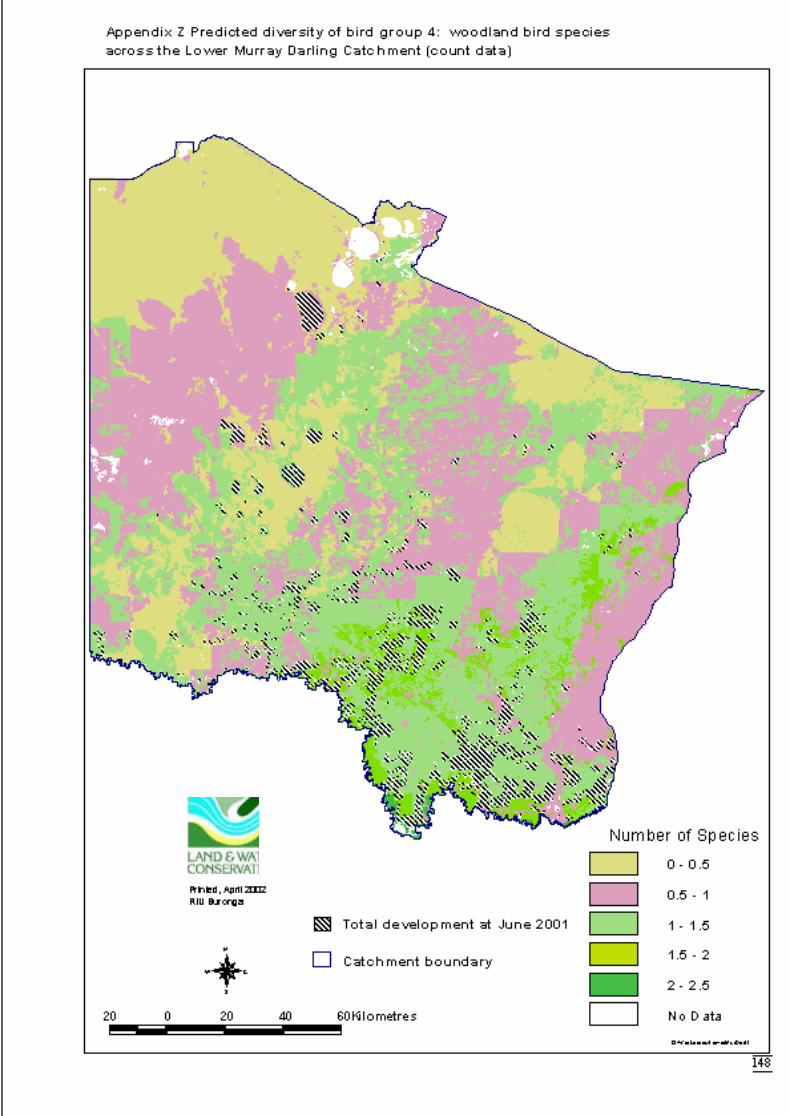
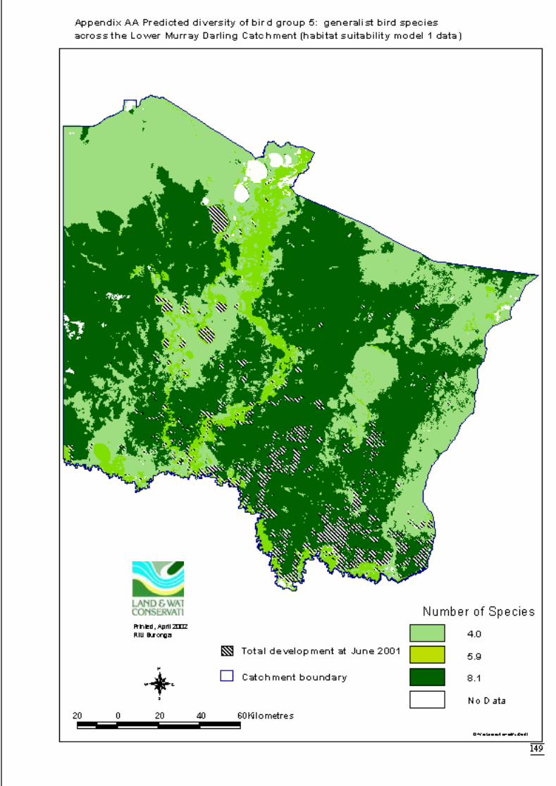
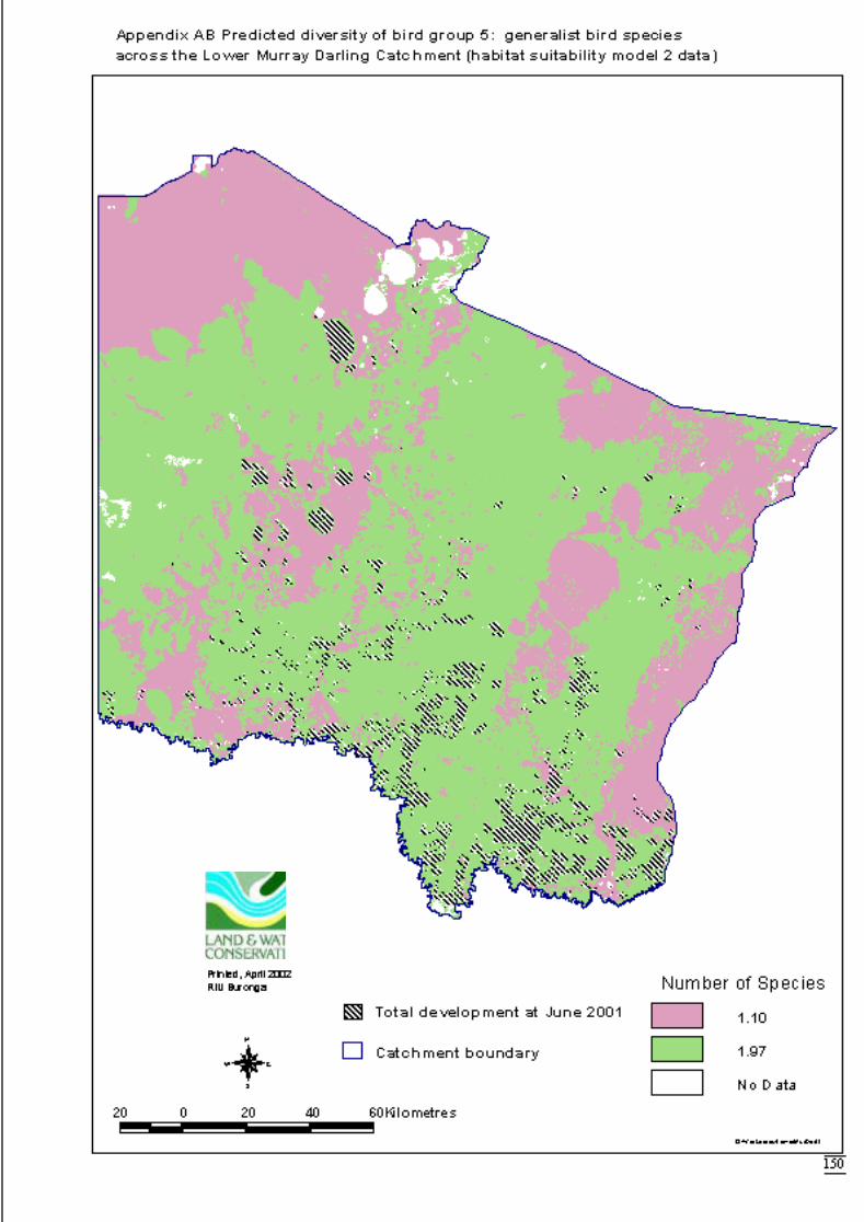
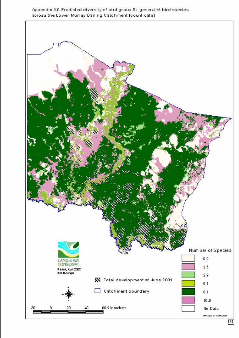
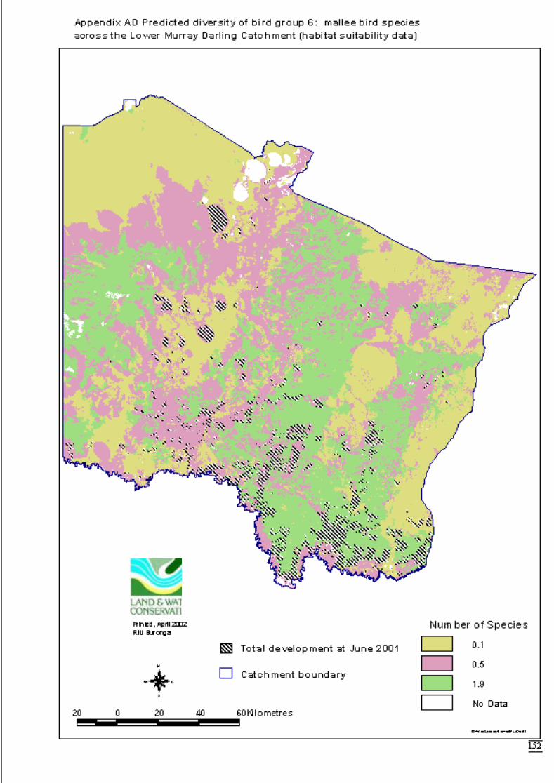
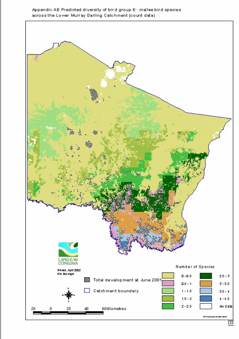
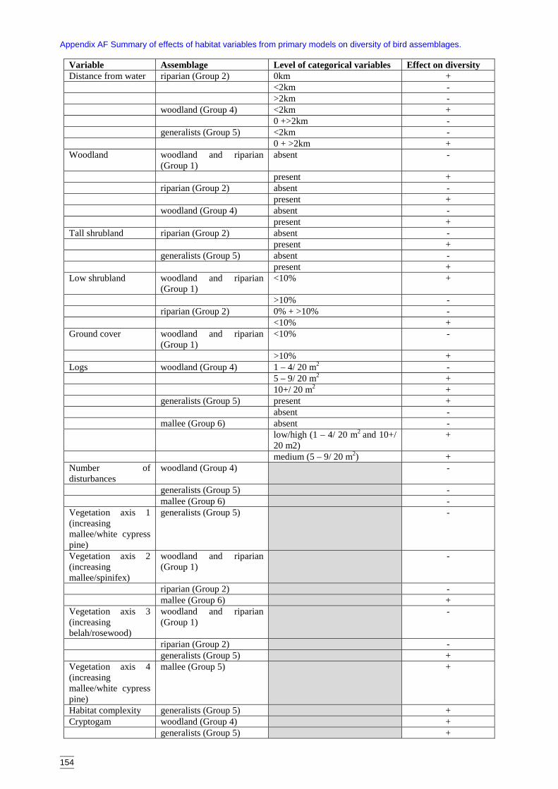
154
Appendix AF Summary of effects of habitat variables from primary models on diversity of bird assemblages.
Variable Assemblage Level of categorical variables Effect on diversityDistance from water riparian (Group 2) 0km +
<2km ->2km -
woodland (Group 4) <2km +0 +>2km -
generalists (Group 5) <2km -0 + >2km +
Woodland woodland and riparian(Group 1)
absent -
present +riparian (Group 2) absent -
present +woodland (Group 4) absent -
present +Tall shrubland riparian (Group 2) absent -
present +generalists (Group 5) absent -
present +Low shrubland woodland and riparian
(Group 1)<10% +
>10% -riparian (Group 2) 0% + >10% -
<10% +Ground cover woodland and riparian
(Group 1)<10% -
>10% +Logs woodland (Group 4) 1 – 4/ 20 m2 -
5 – 9/ 20 m2 +10+/ 20 m2 +
generalists (Group 5) present +absent -
mallee (Group 6) absent -low/high (1 – 4/ 20 m2 and 10+/20 m2)
+
medium (5 – 9/ 20 m2) +Number ofdisturbances
woodland (Group 4) -
generalists (Group 5) -mallee (Group 6) -
Vegetation axis 1(increasingmallee/white cypresspine)
generalists (Group 5) -
Vegetation axis 2(increasingmallee/spinifex)
woodland and riparian(Group 1)
-
riparian (Group 2) -mallee (Group 6) +
Vegetation axis 3(increasingbelah/rosewood)
woodland and riparian(Group 1)
-
riparian (Group 2) -generalists (Group 5) +
Vegetation axis 4(increasingmallee/white cypresspine)
mallee (Group 5) +
Habitat complexity generalists (Group 5) +Cryptogam woodland (Group 4) +
generalists (Group 5) +
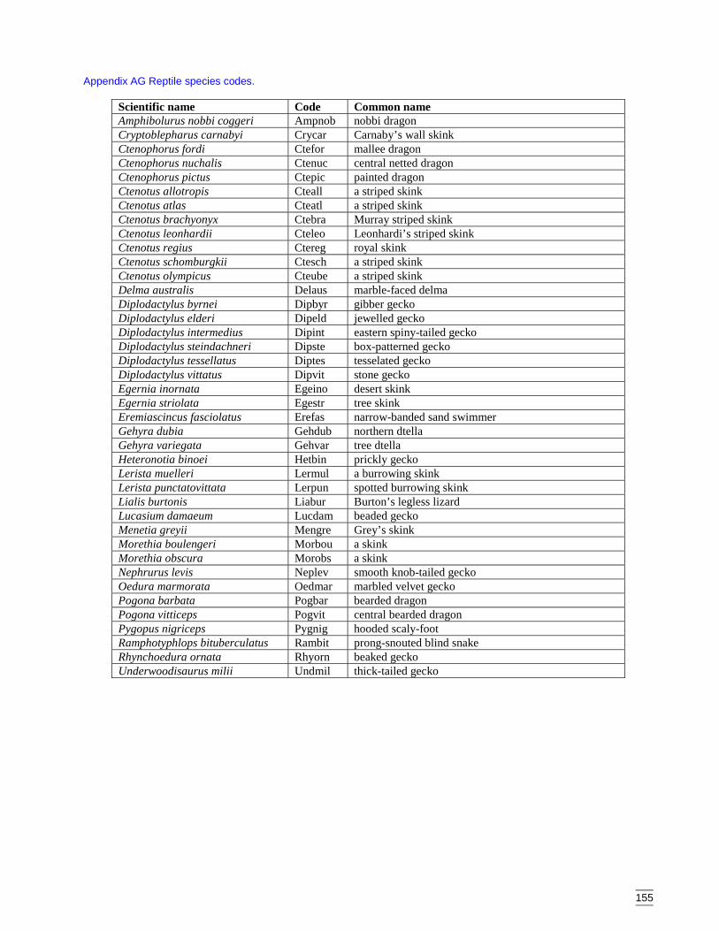
155
Appendix AG Reptile species codes.
Scientific name Code Common nameAmphibolurus nobbi coggeri Ampnob nobbi dragonCryptoblepharus carnabyi Crycar Carnaby’s wall skinkCtenophorus fordi Ctefor mallee dragonCtenophorus nuchalis Ctenuc central netted dragonCtenophorus pictus Ctepic painted dragonCtenotus allotropis Cteall a striped skinkCtenotus atlas Cteatl a striped skinkCtenotus brachyonyx Ctebra Murray striped skinkCtenotus leonhardii Cteleo Leonhardi’s striped skinkCtenotus regius Ctereg royal skinkCtenotus schomburgkii Ctesch a striped skinkCtenotus olympicus Cteube a striped skinkDelma australis Delaus marble-faced delmaDiplodactylus byrnei Dipbyr gibber geckoDiplodactylus elderi Dipeld jewelled geckoDiplodactylus intermedius Dipint eastern spiny-tailed geckoDiplodactylus steindachneri Dipste box-patterned geckoDiplodactylus tessellatus Diptes tesselated geckoDiplodactylus vittatus Dipvit stone geckoEgernia inornata Egeino desert skinkEgernia striolata Egestr tree skinkEremiascincus fasciolatus Erefas narrow-banded sand swimmerGehyra dubia Gehdub northern dtellaGehyra variegata Gehvar tree dtellaHeteronotia binoei Hetbin prickly geckoLerista muelleri Lermul a burrowing skinkLerista punctatovittata Lerpun spotted burrowing skinkLialis burtonis Liabur Burton’s legless lizardLucasium damaeum Lucdam beaded geckoMenetia greyii Mengre Grey’s skinkMorethia boulengeri Morbou a skinkMorethia obscura Morobs a skinkNephrurus levis Neplev smooth knob-tailed geckoOedura marmorata Oedmar marbled velvet geckoPogona barbata Pogbar bearded dragonPogona vitticeps Pogvit central bearded dragonPygopus nigriceps Pygnig hooded scaly-footRamphotyphlops bituberculatus Rambit prong-snouted blind snakeRhynchoedura ornata Rhyorn beaked geckoUnderwoodisaurus milii Undmil thick-tailed gecko
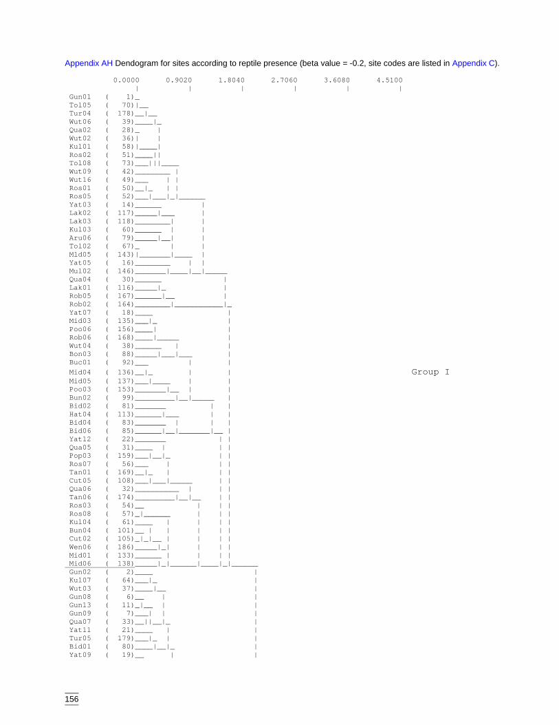
156
Appendix AH Dendogram for sites according to reptile presence (beta value = -0.2, site codes are listed in Appendix C).
0.0000 0.9020 1.8040 2.7060 3.6080 4.5100 | | | | | | Gun01 ( 1)_ Tol05 ( 70)|__ Tur04 ( 178)__|__ Wut06 ( 39)____|_ Qua02 ( 28)_ | Wut02 ( 36)| | Kul01 ( 58)|____| Ros02 ( 51)____|| Tol08 ( 73)___|||____ Wut09 ( 42)________ | Wut16 ( 49)___ | | Ros01 ( 50)__|_ | | Ros05 ( 52)___|___|_|______ Yat03 ( 14)______ | Lak02 ( 117)_____|___ | Lak03 ( 118)________| | Kul03 ( 60)______ | | Aru06 ( 79)_____|__| | Tol02 ( 67)_ | | Mld05 ( 143)|_______|____ | Yat05 ( 16)________ | | Mul02 ( 146)_______|____|__|_____ Qua04 ( 30)______ | Lak01 ( 116)_____|_ | Rob05 ( 167)______|__ | Rob02 ( 164)________|___________|_ Yat07 ( 18)____ | Mid03 ( 135)___|_ | Poo06 ( 156)____| | Rob06 ( 168)____|_____ | Wut04 ( 38)______ | | Bon03 ( 88)_____|___|___ | Buc01 ( 92)___ | | Mid04 ( 136)__|_ | | Group I Mid05 ( 137)___|____ | | Poo03 ( 153)_______|__ | | Bun02 ( 99)_________|__|_____ | Bid02 ( 81)_______ | | Hat04 ( 113)______|___ | | Bid04 ( 83)_______ | | | Bid06 ( 85)______|__|_______|__ | Yat12 ( 22)_______ | | Qua05 ( 31)____ | | | Pop03 ( 159)___|__|_ | | Ros07 ( 56)___ | | | Tan01 ( 169)__|_ | | | Cut05 ( 108)___|___|_____ | | Qua06 ( 32)__________ | | | Tan06 ( 174)_________|__|__ | | Ros03 ( 54)__ | | | Ros08 ( 57)_|______ | | | Kul04 ( 61)____ | | | | Bun04 ( 101)__ | | | | | Cut02 ( 105)_|_|__ | | | | Wen06 ( 186)_____|_| | | | Mid01 ( 133)______ | | | | Mid06 ( 138)_____|_|______|____|_|______ Gun02 ( 2)____ | Kul07 ( 64)___|_ | Wut03 ( 37)____|__ | Gun08 ( 6)__ | | Gun13 ( 11)_|__ | | Gun09 ( 7)___| | | Qua07 ( 33)__||__|_ | Yat11 ( 21)____ | | Tur05 ( 179)___|_ | | Bid01 ( 80)____|__|_ | Yat09 ( 19)__ | |
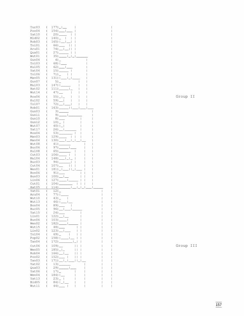
157
Tur03 ( 177)_|__ | | Poo04 ( 154)___|___ | | Yat10 ( 20)____ | | | Mld02 ( 140)_ | | | | Rob03 ( 165)|__|__| | | Tol01 ( 66)___ || | | Aru01 ( 74)__|__|| | | Qua01 ( 27)_____ | | | Wut01 ( 35)____|_|_|______ | Gun04 ( 4)_ | | Tol03 ( 68)|___ | | Kul05 ( 62)___|___ | | Yat04 ( 15)_____ | | | Tol06 ( 71)_ | | | | Man05 ( 131)|___|_|____ | | Gun07 ( 5)_ | | | Mul03 ( 147)|_____ | | | Hat02 ( 111)_____|_ | | | Wut14 ( 47)__ | | | | Ros06 ( 55)_|_ | | | | Group II Kul02 ( 59)__| | | | | Tol07 ( 72)__|___| | | | Rob01 ( 163)_____||___|___|___ | Gun03 ( 3)_____ | | Gun11 ( 9)____|_______ | | Gun10 ( 8)___ | | | Gun12 ( 10)_ | | | | Wut07 ( 40)|_| | | | Yat17 ( 26)__|______ | | | Ros04 ( 53)_______ | | | | Man03 ( 129)____ | | | | | Man04 ( 130)___|__|_|__|__ | | Wut08 ( 41)______ | | | Buc06 ( 97)_____|___ | | | Kul08 ( 65)______ | | | | Cut03 ( 106)____ | | | | | Mul04 ( 148)___|_|_ | | | | Buc03 ( 94)______| | | | | Cut04 ( 107)__ || | | | | Wen01 ( 181)_|___||_|___ | | | Bon06 ( 91)___ | | | | Bun03 ( 100)__|__ | | | | Lin06 ( 127)____|_____ | | | | Cut01 ( 104)_______ | | | | | Hat05 ( 114)______|__|_|_|___|_____ | Yat01 ( 12)_ | | Aru04 ( 77)|____ | | Wut10 ( 43)_ | | | Wut13 ( 46)|___|__ | | Bon04 ( 89)___ | | | Buc05 ( 96)__|___|_____ | | Yat15 ( 24)___ | | | Lin01 ( 122)__|__ | | | Bun06 ( 103)____| | | | Wen02 ( 182)____|_____ | | | Wut15 ( 48)___ | | | | Lin02 ( 123)__|___ | | | | Tol04 ( 69)_ | | | | | Pop02 ( 158)|____|__ | | | | Tan04 ( 172)_______|_| | | | Cut06 ( 109)__ || | | | Group III Wen05 ( 185)_|_ || | | | Rob04 ( 166)__|__ || | | | Poo02 ( 152)___ | || | | | Tan03 ( 171)__|_|___||_|__ | | Yat02 ( 13)______ | | | Qua03 ( 29)_____|___ | | | Yat06 ( 17)_ | | | | Wen04 ( 184)|__ | | | | Yat13 ( 23)_ | | | | | Bid05 ( 84)|_|__ | | | | Wut11 ( 44)___ | | | | |

158
Poo01 ( 151)__|_| | | | | Lin04 ( 125)___||___| | | | Yat16 ( 25)______ | | | | Qua08 ( 34)_____|__|____|________|____|____________ Wut12 ( 45)______ | Lin03 ( 124)_____|_____ | Man02 ( 128)_ | | Group IV Mld04 ( 142)| | | Mul01 ( 145)|_________|____________________________|_ Bon01 ( 86)______ | Mid02 ( 134)_____|___ | Hat06 ( 115)________|___ | Bon02 ( 87)______ | | Mld03 ( 141)_____|_____|_________ | Group V Hat03 ( 112)______ | | Lak04 ( 119)_____|__ | | Mld06 ( 144)_______|_____ | | Pop01 ( 157)_______ | | | Wen03 ( 183)______|_____|_______|___________________|____________________ Kul06 ( 63)_________ | Bun01 ( 98)____ | | Pop04 ( 160)___|____|_ | Aru02 ( 75)________ | | Tur06 ( 180)_______|_|_______ | Aru03 ( 76)_ | | Lak05 ( 120)| | | Lak06 ( 121)|_______ | | Tan02 ( 170)____ | | | Tur01 ( 175)___|___|____ | | Buc02 ( 93)_______ | | | Tan05 ( 173)______|_ | | | Buc04 ( 95)____ | | | | Group VI Mul05 ( 149)___|___|___|___ | | Aru05 ( 78)______ | | | Man06 ( 132)____ | | | | Poo05 ( 155)___|_|__ | | | Mld01 ( 139)_______|__ | | | Bid03 ( 82)____ | | | | Hat01 ( 110)___| | | | | Tur02 ( 176)__||_ | | | | Pop05 ( 161)____|____|___ | | | Bon05 ( 90)_ | | | | Pop06 ( 162)|_____ | | | | Mul06 ( 150)_____|____ | | | | Bun05 ( 102)_______ | | | | | Lin05 ( 126)______|__|__|_|_|___________________________________________| | | | | | | 0.0000 0.9020 1.8040 2.7060 3.6080 4.5100
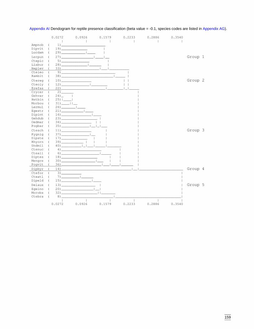
159
Appendix AI Dendogram for reptile presence classification (beta value = -0.1, species codes are listed in Appendix AG).
0.0272 0.0926 0.1579 0.2233 0.2886 0.3540 | | | | | | Ampnob ( 1)______________________ Dipvit ( 19)_____________ | Lucdam ( 29)____________|____ | Lerpun ( 27)________________|____|__ Group 1 Ctepic ( 5)______________ | Liabur ( 28)_____________|______ | Neplev ( 33)___________________|___|__________ Cteleo ( 9)___________________________ | Rambit ( 38)__________________________|_____ | Ctereg ( 10)_______________ | | Group 2 Cteoly ( 12)______________|________ | | Erefas ( 22)______________________|________|_|_____ Crycar ( 2)______ | Gehvar ( 24)_ | | Hetbin ( 25)|____| | Morbou ( 31)____||__ | Lermul ( 26)_______|____ | Egestr ( 21)___________|____ | Dipint ( 16)_______________|____ | Gehdub ( 23)__________________ | | Oedmar ( 34)_______________ | | | Pogbar ( 35)______________|__|_|___ | Ctesch ( 11)_______________ | | Group 3 Pygnig ( 37)______________|__ | | Dipste ( 17)_____________ | | | Rhyorn ( 39)___________ | | | | Undmil ( 40)__________|_|___|_____|_______ | Ctenuc ( 4)____________________ | | Cteall ( 6)___________________|_____ | | Diptes ( 18)__________________ | | | Mengre ( 30)_________________|___ | | | Pogvit ( 36)____________________|___|____|______ | Dipbyr ( 14)___________________________________|__|______________________ Group 4 Ctefor ( 3)__________ | Cteatl ( 7)_________|______ | Dipeld ( 15)_______________|____ | Delaus ( 13)_________________ | | Group 5 Egeino ( 20)________________|__| | Morobs ( 32)__________________||_______ | Ctebra ( 8)__________________________|_________________________________| | | | | | | 0.0272 0.0926 0.1579 0.2233 0.2886 0.3540
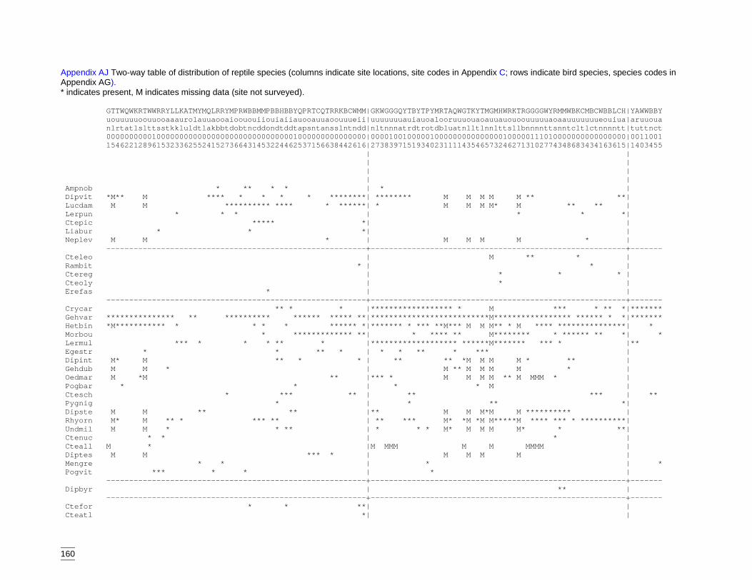
160
Appendix AJ Two-way table of distribution of reptile species (columns indicate site locations, site codes in Appendix C; rows indicate bird species, species codes inAppendix AG).* indicates present, M indicates missing data (site not surveyed).
GTTWQWKRTWWRRYLLKATMYMQLRRYMPRWBBMMPBBHBBYQPRTCQTRRKBCWMM|GKWGGGQYTBYTPYMRTAQWGTKYTMGMHWRKTRGGGGWYRMMWBKCMBCWBBLCH|YAWWBBY uouuuuuoouuooaaaurolauuaooaioououiiouiaiiauooauuaoouuueii|uuuuuuuauiauoalooruuuouaoauuauouoouuuuuaoaauuuuuuueouiua|aruuoua nlrtatlslttsstkkluldtlakbbtdobtncddondtddtapsntansslntndd|nltnnnatrdtrotdbluatnlltlnnlttsllbnnnnttsnntcltlctnnnntt|tuttnct 000000000010000000000000000000000000000001000000000000000|00001001000001000000000000000100000111010000000000000000|0011001 154622128961532336255241527366431453224462537156638442616|27383971519340231111435465732462713102774348683434163615|1403455 | | | | | | | | Ampnob * ** * * | * | Dipvit *M** M **** * * * * ********| ******** M M M M M ** **| Lucdam M M ********** **** * ******| * M M M M* M ** ** | Lerpun * * * | * * *| Ctepic ***** *| | Liabur * * *| | Neplev M M * | M M M M * | ---------------------------------------------------------+--------------------------------------------------------+------- Cteleo | M ** * | Rambit * | * | Ctereg | * * * | Cteoly | * | Erefas * | | ---------------------------------------------------------+--------------------------------------------------------+------- Crycar ** * * |****************** * M *** * ** *|******* Gehvar *************** ** ********** ****** ***** **|**************************M***************** ****** * *|******* Hetbin *M*********** * * * * ****** *|******* * *** **M*** M M M** * M **** ***************| * Morbou * ************* **| * **** ** M******** * ****** ** *| * Lermul *** * * * ** * |******************* ******M******* *** * |** Egestr * * ** * | * * ** * *** | Dipint M* M ** * * | ** ** *M M M M * ** | Gehdub M M * | M ** M M M M * | Oedmar M *M ** |*** * M M M M ** M MMM * | Pogbar * * | * * M | Ctesch * *** ** | ** *** | ** Pygnig * | * ** *| Dipste M M ** ** |** M M M*M M ********** | Rhyorn M* M ** * *** ** | ** *** M* *M *M M*****M **** *** * **********| Undmil M M * * ** | * * * M* M M M M* * **| Ctenuc * * | * | Cteall M * |M MMM M M MMMM | Diptes M M *** * | M M M M | Mengre * * | * | * Pogvit *** * * | * | ---------------------------------------------------------+--------------------------------------------------------+------- Dipbyr | ** | ---------------------------------------------------------+--------------------------------------------------------+------- Ctefor * * **| | Cteatl *| |
161
Dipeld | | Delaus | | Egeino | | Morobs | | Ctebra | |

162
LBWWLTPTCWRPTYQYWYBWPLYQ|WLMMM|BMHBMHLMPW|KBPATALLTTBTBMAMPMBHTPBPMBL iueuiooaueooaauaeaiuoiau|uialu|oiaolaaloe|uuoruraaauuauuraoliauooouui nnntnlpntnbontatntdtonta|tnndl|ndtndtkdpn|lnpurukknrcnclunoddtrpnplnn 000100000000000001010010|10000|0000000000|000000000000000000000000000 162524246542323643511468|23241|1262334613|614263562125455651312556655 | | | | | | | | | | | | Ampnob | | | * ** Dipvit M **| | *| * * * ** Lucdam * **M* * | | | ************ ******** Lerpun * ** * | | | *** * Ctepic | | | * Liabur | | | ** Neplev M | | |* * ------------------------+-----+----------+--------------------------- Cteleo | |* | Rambit | | | Ctereg | |***** * | *** * Cteoly | | ** **| Erefas * | |** | ------------------------+-----+----------+--------------------------- Crycar ************************|** | | Gehvar *********************** | | |* * Hetbin **M***** ***** | | | Morbou **** ** ** *** ** * | | * | * * Lermul * | | | * Egestr **********| | | Dipint M ** * | | | * Gehdub M | | | Oedmar M * | | | Pogbar | | | Ctesch | | * **| Pygnig | | * *| Dipste M | | * | Rhyorn * M* * | |*** | **** * Undmil M | |* * * | Ctenuc | | | Cteall ** * | | | Diptes M ***** | ****| | Mengre ** * | | | Pogvit | | | ------------------------+-----+----------+--------------------------- Dipbyr | | | ------------------------+-----+----------+--------------------------- Ctefor | | |******** * *************** Cteatl | | |* * ** **** Dipeld | | | ******
163
Delaus | | | ** Egeino | | | **** Morobs | | | ** Ctebra | | | * *

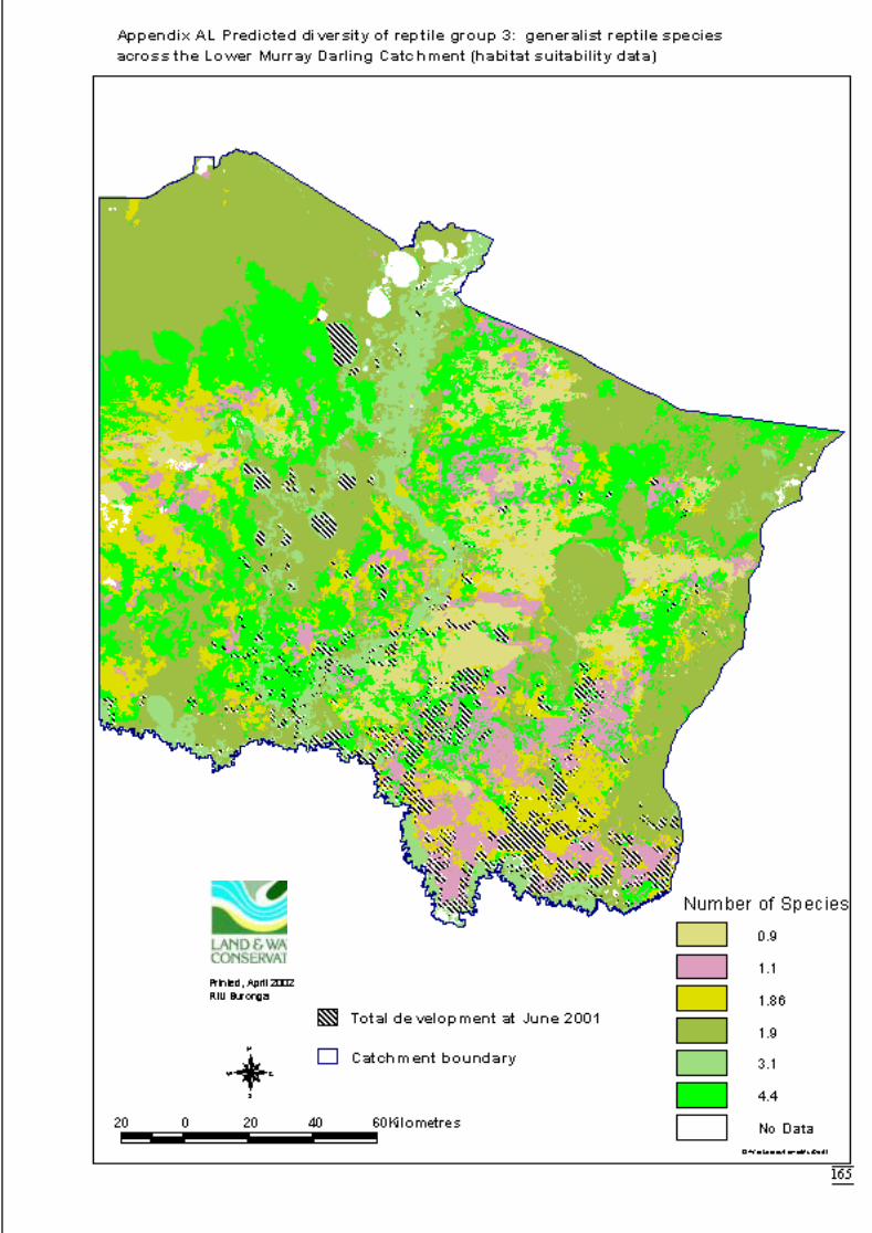
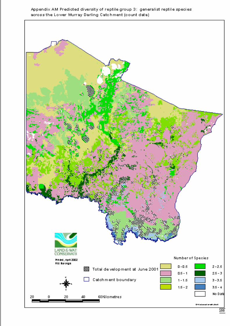
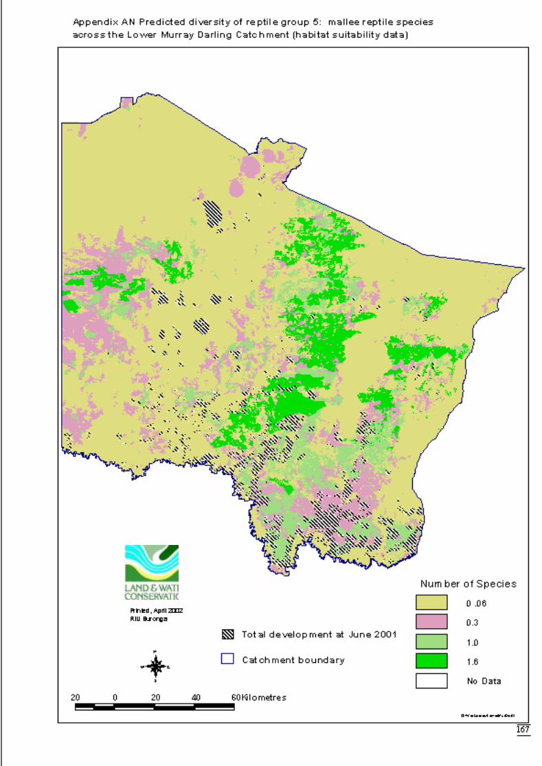
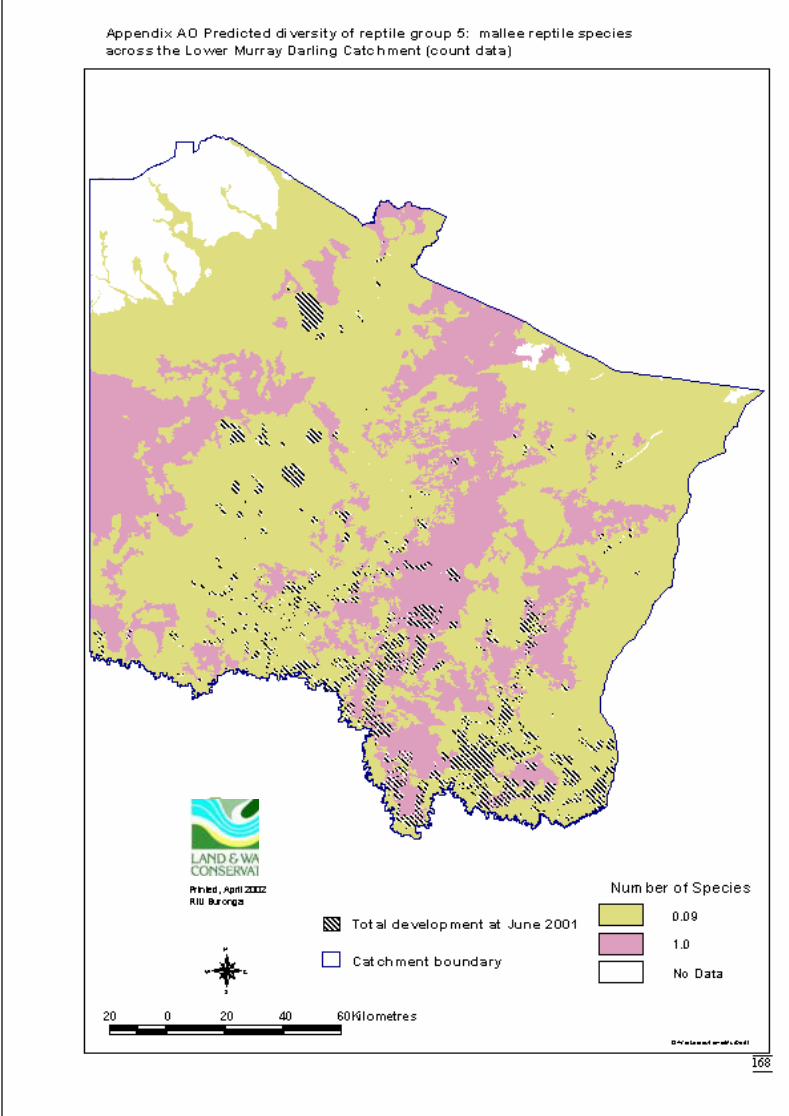
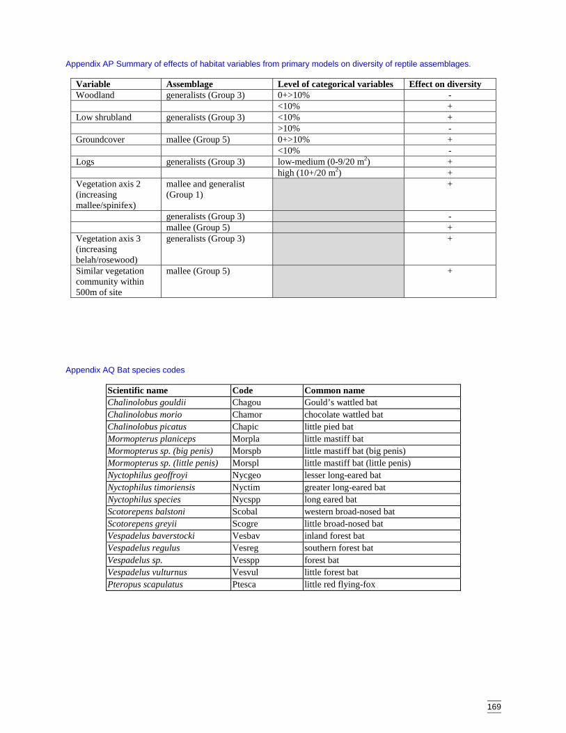
169
Appendix AP Summary of effects of habitat variables from primary models on diversity of reptile assemblages.
Variable Assemblage Level of categorical variables Effect on diversityWoodland generalists (Group 3) 0+>10% -
<10% +Low shrubland generalists (Group 3) <10% +
>10% -Groundcover mallee (Group 5) 0+>10% +
<10% -Logs generalists (Group 3) low-medium (0-9/20 m2) +
high (10+/20 m2) +Vegetation axis 2(increasingmallee/spinifex)
mallee and generalist(Group 1)
+
generalists (Group 3) -mallee (Group 5) +
Vegetation axis 3(increasingbelah/rosewood)
generalists (Group 3) +
Similar vegetationcommunity within500m of site
mallee (Group 5) +
Appendix AQ Bat species codes
Scientific name Code Common nameChalinolobus gouldii Chagou Gould’s wattled batChalinolobus morio Chamor chocolate wattled batChalinolobus picatus Chapic little pied batMormopterus planiceps Morpla little mastiff batMormopterus sp. (big penis) Morspb little mastiff bat (big penis)Mormopterus sp. (little penis) Morspl little mastiff bat (little penis)Nyctophilus geoffroyi Nycgeo lesser long-eared batNyctophilus timoriensis Nyctim greater long-eared batNyctophilus species Nycspp long eared batScotorepens balstoni Scobal western broad-nosed batScotorepens greyii Scogre little broad-nosed batVespadelus baverstocki Vesbav inland forest batVespadelus regulus Vesreg southern forest batVespadelus sp. Vesspp forest batVespadelus vulturnus Vesvul little forest batPteropus scapulatus Ptesca little red flying-fox
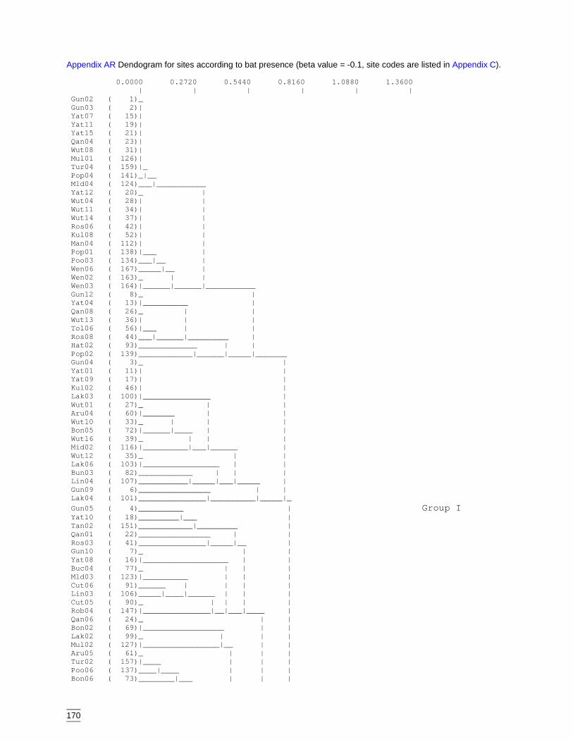
170
Appendix AR Dendogram for sites according to bat presence (beta value = -0.1, site codes are listed in Appendix C).
0.0000 0.2720 0.5440 0.8160 1.0880 1.3600 | | | | | | Gun02 ( 1)_ Gun03 ( 2)| Yat07 ( 15)| Yat11 ( 19)| Yat15 ( 21)| Qan04 ( 23)| Wut08 ( 31)| Mul01 ( 126)| Tur04 ( 159)|_ Pop04 ( 141)_|__ Mld04 ( 124)___|___________ Yat12 ( 20)_ | Wut04 ( 28)| | Wut11 ( 34)| | Wut14 ( 37)| | Ros06 ( 42)| | Kul08 ( 52)| | Man04 ( 112)| | Pop01 ( 138)|___ | Poo03 ( 134)___|__ | Wen06 ( 167)_____|__ | Wen02 ( 163)_ | | Wen03 ( 164)|______|______|___________ Gun12 ( 8)_ | Yat04 ( 13)|__________ | Qan08 ( 26)_ | | Wut13 ( 36)| | | Tol06 ( 56)|___ | | Ros08 ( 44)___|______|_________ | Hat02 ( 93)_____________ | | Pop02 ( 139)____________|______|_____|_______ Gun04 ( 3)_ | Yat01 ( 11)| | Yat09 ( 17)| | Kul02 ( 46)| | Lak03 ( 100)|_______________ | Wut01 ( 27)_ | | Aru04 ( 60)|_______ | | Wut10 ( 33)_ | | | Bon05 ( 72)|______|____ | | Wut16 ( 39)_ | | | Mid02 ( 116)|__________|___|______ | Wut12 ( 35)_ | | Lak06 ( 103)|_________________ | | Bun03 ( 82)____________ | | | Lin04 ( 107)___________|_____|___|_____ | Gun09 ( 6)________________ | | Lak04 ( 101)_______________|__________|_____|_ Gun05 ( 4)__________ | Group I Yat10 ( 18)_________|___ | Tan02 ( 151)____________|_________ | Qan01 ( 22)________________ | | Ros03 ( 41)_______________|_____|__ | Gun10 ( 7)_ | | Yat08 ( 16)|___________________ | | Buc04 ( 77)_ | | | Mld03 ( 123)|__________ | | | Cut06 ( 91)______ | | | | Lin03 ( 106)_____|____|______ | | | Cut05 ( 90)_ | | | | Rob04 ( 147)|_______________|__|___|____ | Qan06 ( 24)_ | | Bon02 ( 69)|__________________ | | Lak02 ( 99)_ | | | Mul02 ( 127)|_________________|__ | | Aru05 ( 61)_ | | | Tur02 ( 157)|____ | | | Poo06 ( 137)____|____ | | | Bon06 ( 73)________|___ | | |

171
Cut01 ( 86)_ | | | | Wen04 ( 165)|__________| | | | Rob01 ( 144)__________||________|______|____ | Wut06 ( 30)_________________ | | Hat01 ( 92)________ | | | Tur06 ( 161)_______|________|_________ | | Kul03 ( 47)_ | | | Tan03 ( 152)|_____ | | | Rob02 ( 145)_____|____ | | | Tol02 ( 54)_________|________ | | | Mld05 ( 125)_________________|_______|_____|_|___________________________ Gun08 ( 5)____ | Bun04 ( 83)___|__ | Man03 ( 111)_____|__ | Mid04 ( 118)____ | | Poo04 ( 135)___|___|__________ | Kul07 ( 51)________ | | Hat05 ( 96)_______|_____ | | Bon01 ( 68)______ | | | Cut04 ( 89)_____|______|____|_______ | Tol01 ( 53)_ | | Tol03 ( 55)| | | Tol08 ( 57)|___________________ | | Buc03 ( 76)_____ | | | Tur03 ( 158)____|_____ | | | Man05 ( 113)_________|_________|____|____ | Aru02 ( 58)___________ | | Poo01 ( 132)__________|____ | | Buc01 ( 74)_____ | | | Poo05 ( 136)____|______ | | | Bun06 ( 85)__________|___|_____ | | Bid01 ( 62)________ | | | Bid05 ( 66)_____ | | | | Mid05 ( 119)____|__|__ | | | Mid03 ( 117)_ | | | | Mid06 ( 120)|________|__ | | | Bid06 ( 67)_ | | | | Tur05 ( 160)|___ | | | | Lin06 ( 109)___|____ | | | | Rob05 ( 148)_______|___| | | | Group II Buc06 ( 79)_ | | | | Hat04 ( 95)|______ | | | | Mul04 ( 129)______|____|_______|__ | | Bid02 ( 63)_ | | | Lin01 ( 104)|__ | | | Bid04 ( 65)__|___ | | | Tan04 ( 153)_____|__ | | | Wen05 ( 166)_______|____ | | | Buc02 ( 75)____ | | | | Mid01 ( 115)_ | | | | | Rob06 ( 149)|__|_____ | | | | Poo02 ( 133)________|__|___ | | | Bon04 ( 71)____ | | | | Hat06 ( 97)___|___ | | | | Cut02 ( 87)___ | | | | | Mul03 ( 128)__|__ | | | | | Cut03 ( 88)_ | | | | | | Pop05 ( 142)|___| | | | | | Lin02 ( 105)___||_|_____ | | | | Buc05 ( 78)____ | | | | | Mul06 ( 131)___|_ | | | | | Tur01 ( 156)____|_____ | | | | | Pop06 ( 143)_________|_|__|__ | | | Mld02 ( 122)__________ | | | | Wen01 ( 162)_________|______|____|______|_______________ | Gun13 ( 9)_______ | | Gun15 ( 10)_ | | | Yat06 ( 14)|_____|__ | | Bun02 ( 81)_____ | | | Bun05 ( 84)____|___|___ | | Bid03 ( 64)___________|_______ | | Yat03 ( 12)_ | | | Wut05 ( 29)| | | |
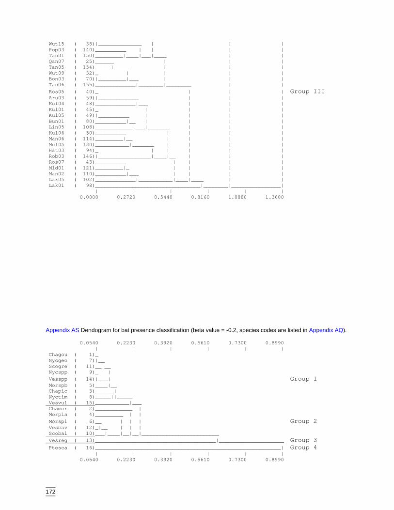
172
Wut15 ( 38)|______________ | | | Pop03 ( 140)__________ | | | | Tan01 ( 150)_________|____|___|____ | | Qan07 ( 25)______ | | | Tan05 ( 154)_____|_____ | | | Wut09 ( 32)_ | | | | Bon03 ( 70)|_________|___ | | | Tan06 ( 155)_____________|________|________ | | Ros05 ( 40)_ | | | Group III Aru03 ( 59)|_____________ | | | Kul04 ( 48)_____________|___ | | | Kul01 ( 45)_ | | | | Kul05 ( 49)|__________ | | | | Bun01 ( 80)__________|__ | | | | Lin05 ( 108)____________|___|_______ | | | Kul06 ( 50)__________ | | | | Man06 ( 114)_________|__ | | | | Mul05 ( 130)___________|_______ | | | | Hat03 ( 94)_ | | | | | Rob03 ( 146)|_________________|____|__ | | | Ros07 ( 43)__________ | | | | Mld01 ( 121)_________|_ | | | | Man02 ( 110)__________|___ | | | | Lak05 ( 102)_____________|___________|____|____ | | Lak01 ( 98)__________________________________|________|________________| | | | | | | 0.0000 0.2720 0.5440 0.8160 1.0880 1.3600
Appendix AS Dendogram for bat presence classification (beta value = -0.2, species codes are listed in Appendix AQ).
0.0540 0.2230 0.3920 0.5610 0.7300 0.8990 | | | | | | Chagou ( 1)_ Nycgeo ( 7)|__ Scogre ( 11)__|__ Nycspp ( 9)_ | Vesspp ( 14)|___| Group 1 Morspb ( 5)____|__ Chapic ( 3)______| Nyctim ( 8)_____||_____ Vesvul ( 15)___________|___ Chamor ( 2)____________ | Morpla ( 4)_________ | | Morspl ( 6)__ | | | Group 2 Vesbav ( 12)_|__ | | | Scobal ( 10)___|____|__|__|_________________________ Vesreg ( 13)_______________________________________|_____________________ Group 3 Ptesca ( 16)____________________________________________________________| Group 4 | | | | | | 0.0540 0.2230 0.3920 0.5610 0.7300 0.8990
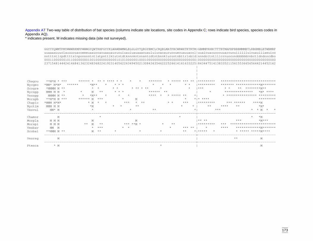
173
Appendix AT Two-way table of distribution of bat species (columns indicate site locations, site codes in Appendix C; rows indicate bird species, species codes inAppendix AQ).* indicates present, M indicates missing data (site not surveyed).
GGYYYQWMTPMYWWWRKMPPWWWGYQWTRHPGYYKLWAWBWMWLBLGLGYTQRGYBMCLCRQBLMATPBCWRWHTKTRTM|GBMMPKHBCTTTBTMAPBPBBBMMMBTLRBHMBLBTWBMRP uuaaaauuuolauuuouaooeeeuaauooaouaauauruouiuauiuauaaaouauluiuoaoauruooueouauuaool|uuaiouaouooouuarououiiiiiiuiouauiiiaeuioo nntttntlrpdttttslnponnnntntlstpnttlktutntdtknnnkntnnsntcdtntbnnklurontnbttrlnbld|nnndoltntlllcrnuoconddddddrnbctldndnncdbo 00011000000101100000000100100000000000101010000001000100000000000000000000000000|00000000000000000000000000000000000000000 23715481444241468413623248368224192314056226349450213084363546222526614161633225|84344751413833521156155366565644214452162 | | | | Chagou **M*M * *** ****** * ** * **** * * * * ******* * ***** *** ** |********* ***************************** Nycgeo *MM* M*M* ****** *M** * * * * * * * * * |********* ******* *************M******* Scogre *MMMM M ** * * * * * ** * ** * * |*** * * ** ********M** Nycspp MMM M M * * M ** * * * ****** ** | * *************** *M* **** Vesspp MMMM M ** * *M** * * * **** * * ***** ** *| * **************** ********* Morspb **M*M M *** ****** M *** * M * *|* **** ********* Chapic *MMM M*M* * M * * *** * ** * * *** |********* *** ****** ****M Nyctim MMM M M *M * * ** * * | ** **** ** *M* Vesvul MM* M * * ** *| *** * * M * * --------------------------------------------------------------------------------+----------------------------------------- Chamor M * * | * *M Morpla M M M M M |** ** *** *M*** Morspl M M M ** M ** *** **M * * ** |********* *** ************************ Vesbav MM M * *** * * * *** ** | * **** *************M******* Scobal **MMM M ** M ** * * * ** *|***** * * ***** *****M**** --------------------------------------------------------------------------------+----------------------------------------- Vesreg M | ** M --------------------------------------------------------------------------------+----------------------------------------- Ptesca * M * | M
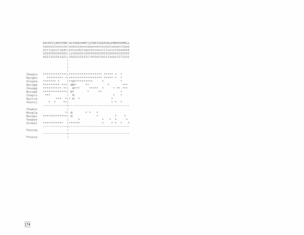
174
BHCMCPLBMTPMW|GGYBBBYWWPTQTWBTRAKKKBLKMMHRRMMLL oauuuoiuuuole|uuauuiauuoaaauoaoruuuuiuauaoolaaa nttltpnclrpdn|nntnndtttpnnntnnsulllnnlnltbsdnkk 0000000000000|110000001000000000000000000000000 4623352561621|356253355317593653415156653371251 | | | | Chagou *************|****************** ***** * * Nycgeo ********* *|****************** ***** * * Scogre ******* * |**M********** * * Nycspp ********* ***| MM* ** * *** Vesspp ********** **| M*** ***** * * ** *** Morspb *************| M* * ** * Chapic *** | M * * Nyctim *** *|* M * * Vesvul * * **| * * * -------------+--------------------------------- Chamor | Morpla *| M * * * Morspl *************| M * * * Vesbav | * * * * * Scobal *********** |****** * * * * * -------------+--------------------------------- Vesreg | -------------+--------------------------------- Ptesca |
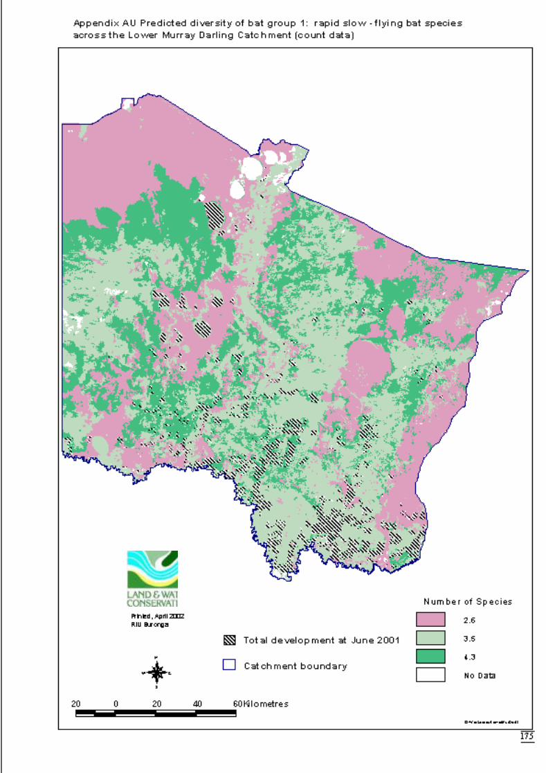
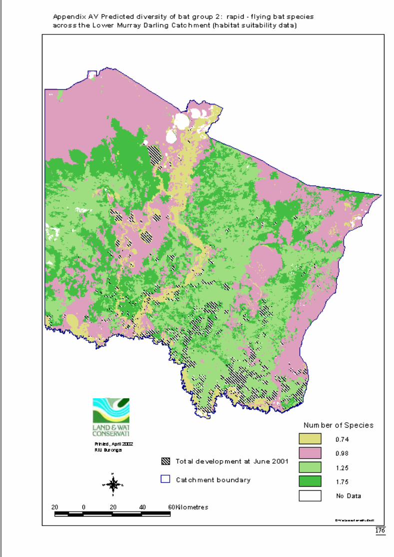
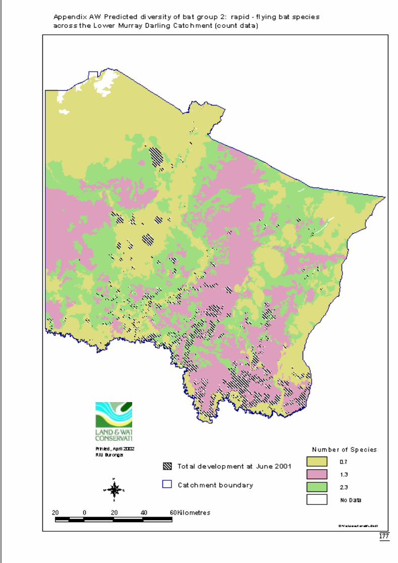
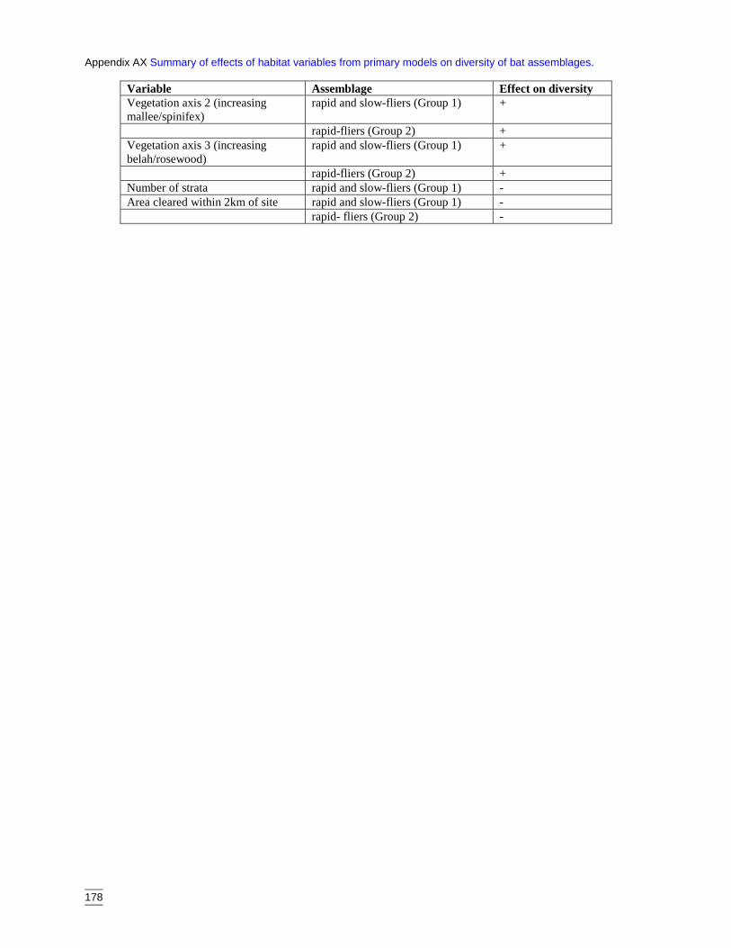
178
Appendix AX Summary of effects of habitat variables from primary models on diversity of bat assemblages.
Variable Assemblage Effect on diversityVegetation axis 2 (increasingmallee/spinifex)
rapid and slow-fliers (Group 1) +
rapid-fliers (Group 2) +Vegetation axis 3 (increasingbelah/rosewood)
rapid and slow-fliers (Group 1) +
rapid-fliers (Group 2) +Number of strata rapid and slow-fliers (Group 1) -Area cleared within 2km of site rapid and slow-fliers (Group 1) -
rapid- fliers (Group 2) -
179
REFERENCESAndrew, M.H. & Lange, R.T. 1986, ‘Development of a new piosphere in arid chenopodshrubland grazed by sheep. I. Changes to the soil surface,’ Aust. J. Ecol., 11, 395 – 409.
Ayers, D., Nash, S. & Baggett, K. (1996 with updates) Threatened species of western New SouthWales, NSW National Parks and Wildlife Service, Hurstville.
Barrett, G.W., Ford, H.A. & Recher, H.F. 1994, ‘Conservation of woodland birds in a fragmentedrural landscape’, Pac. Consv. Biol., 1, 245 – 56.
Belbin, L. 1995, PATN: pattern analysis package (user’s guide), CSIRO Division of WildlifeEcology, Canberra.
Bennett, A.F., Lumsden, L.F. & Menkhorst, P.W. 1989, ‘Mammals of the mallee region ofsoutheastern Australia’, in Noble, J.C. & Bradstock, R.A. (eds) Mediterranean landscapes inAustralia. CSIRO, Australia.
Bos, D.G., Carthew, S.M. & Lorimer, M.F. 2002, ‘Habitat selection by the small dasyuridNingaui yvonneae (Marsupialia: Dasyuridae) in South Australia’, Austral Ecol., 27,103 – 109.
Briggs, S., Seddon, J. & Doyle, S. 2001, Birds in woodland remnants of the central wheat/sheepbelt of New South Wales, Report on NHT project: Predicting biodiversity of woodland remnantsfor on-ground conservation, Canberra.
Calow, P. (ed) 1999, Blackwell’s concise encyclopedia of ecology, Blackwell Sciences Ltd,Carlton, Victoria.
Catling, P.C. & Burt, R.J. 1995, ‘Studies of the ground-dwelling mammals of eucalypt forests insouth-eastern New South Wales: the effect of habitat variables on distribution and abundance’,Wild. Res., 22, 271 - 88.
Catling, P.C. & Burt, R.J. 1997, ‘Studies of the ground-dwelling mammals of eucalypt forests innorth-eastern New South Wales: the species, their abundance and distribution’, Wild. Res., 24,1 –19.
Catling, P.C., Burt, R.J. & Forrester, R.I. 1998, ‘Models of distribution and abundance of ground-dwelling mammals in the eucalypt forests of south-eastern New South Wales’, Wild. Res., 25,449 – 466.
Catling, P.C., Burt, R.J. & Forrester, R.I. 2000, ‘Models of distribution and abundance of ground-dwelling mammals in the eucalypt forests of north-eastern New South Wales in relation to habitatvariables’, Wild. Res., 25, 449 – 466.
Claridge, A. & Barry, S. 2000, ‘Factors influencing the distribution of medium-sized ground-dwelling mammals in south-eastern mainland Australia’, Austral Ecol., 25, 676 – 688.
Claridge, A., Barry, S., Cork, S. & Trappe, J. 2000, ‘ Diversity and habitat relationships ofhypogeous fungi. II. Factors influencing the occurrence and number of taxa’, Biodiv. and Consv.,9, 175 – 199.
180
Christian C.S. 1958, ‘The concept of land units and land systems’, Proc. Ninth Pacific Sci Congr,1957, 20, 74 – 81.
Churchill, S. 1998, Australian bats, Reed New Holland, Sydney.
Cogger, H.G. 1992, Reptiles and amphibians of Australia, Reed Books, Sydney.
Cunningham, G.M., Mulham, W.E., Milthorpe, P.L. & Leigh, J.H. 1992, Plants of western NewSouth Wales, Soil Conservation Service, Sydney.
Cunningham, S.A. 2000, ‘Effects of habitat fragmentation on the reproductive ecology of fourplant species in mallee woodland’, Consv. Biol., 14, 758 – 768.
Dickman, C.R. 1993, The biology and management of native rodents of the arid zone in NSW,species management report number 12, NSW National Parks and Wildlife Service, Hurstville.
Dickman, C.R. & Read, D.G. 1992, The Biology and Management of Dasyurids in the Arid Zonein NSW, Species Management Report Number 11, NSW National Parks and Wildlife Service,Hurstville.
Dickman, C.R., Pressey, R.L., Lim, L. & Parnaby, H.E. 1993, ‘Mammals of particularconservation concern in the western division of New South Wales’, Biol. Consv., 65, 219 – 248.
Dominelli, S. (ed) 1999, Effects of artificial watering points on mallee flora and fauna, Finalreport to Environment Australia, Canberra.
Eldridge, D. & Tozer, M. 1997, A practical guide to soil lichens and bryophytes of Australia’sdry country, Department of Land and Water Conservation, Sydney.
Faith, D.P. & Norris, R.H. 1989, ‘Correlation of environmental variables with patterns ofdistribution and abundance of common and rare freshwater macroinvertebrates’, Biol. Consv., 50,77 – 98.
Ferrier, S. & Watson, G. 1997, An evaluation of the effectiveness of environmental surrogatesand modelling techniques in predicting the distribution of biological diversity, a consultancyreport for Department of Environment, Sport and Territories.
Fisher, C.D., Lindgren, E. & Dawson, W. 1972, ‘Drinking patterns and behaviour of Australiandesert birds in relation to their ecology and abundance’, The Condor 74, 111 – 136.
Ford, H.A., Barrett, G.A., Saunders, D.A. & Recher H.F. 2001, ‘Why have birds in thewoodlands of southern Australia declined?’, Biol. Consv., 97, 71 – 88.
Forward, L.R. & Robinson, A.C. (eds) 1996, A biological survey of the South Olary Plains SouthAustralia 1991-1992, biological survey of South Australia, Department of Environment andNatural Resources, Adelaide.
Foulkes, J., Foster, E. & de Preu, N. 1995, Palaeodrainage systems and the conservation ofAustralian deserts, States Cooperative Assistance Program Project No. 4112, Final report to the
181
Australian Nature Conservation Agency by the Conservation Commission of the NorthernTerritory, Alice Springs.
Fox, B.J. & Fox, M.D., 1981, ‘A comparison of vegetation classifications as descriptors of smallmammal habitat preference’, in Gillison A.N. & Anderson, D.J. (eds) Vegetation classification inAustralia, CSIRO.
Fox, B.J. & McKay, G.M. 1981, ‘Small mammal responses to pyric successional changes ineucalyptus forest’, Aust. J. Ecol., 6,29 – 41.
Goldney, D.C. & Bowie, J.S. 1990, ‘Some management implications for the conservation ofvegetation remnants and associated fauna in the central western region of New South Wales,’Proc. Ecol. Soc. Aust., 16, 427-440.
Green, R.J. & Catterall 1998, ‘The effects of forest clearing and regeneration on the fauna ofWivenhoe Park, south-east Queensland’, Wild. Res., 25, 677 – 690.
Greig, P.J. & Devonshire, P.J. 1981, ‘Tree removals and saline seepage in Victorian catchments:some hydrological and economic results’, Aust. J. Agric. Econ., 25, 134 – 148.
Hadden, S.A. & Westbrooke, M.E. 1996, ‘Habitat relationships of the herpetofauna of remnantbuloke woodlands of the Wimmera Plains, Victoria’, Wild. Res., 23, 363 – 72.
Harden, G.J. (ed) 1990, Flora of New South Wales, vol. 1, New South Wales University Press,Kensington.
Harden, G.J. (ed) 1991, Flora of New South Wales, vol. 2, New South Wales University Press,Kensington.
Harden, G.J. (ed) 1992, Flora of New South Wales, vol. 3, New South Wales University Press,Kensington.
Harden, G.J. (ed) 1993, Flora of New South Wales, vol. 4, New South Wales University Press,Kensington.
Hart, D. 1995, Symbols of western New South Wales plants, Department of Conservation andLand Management, Western Region publication 95/1.
Hodgins, I.W. & Rogers, R.W. 1997, ‘Correlations of stocking with the cryptogamic soil crust ofa semi-arid rangeland in southwest Queensland’, Aust. J. Ecol., 22, 425 – 431.
Insightful 2001, S-PLUS 6 for Windows, Insightful Corporation, Seattle, WA.
James, C., Landsberg, J. & Morton, S. 1995, ‘Ecological functioning in arid Australia andresearch to assist conservation of biodiversity’, Pac. Consv. Biol., 2, 126 – 42.
Jansen, A. & Robertson, A. 2001, ‘Riparian bird communities in relation to land managementpractices in floodplain woodlands of south-eastern Australia,’ Biol. Consv. 100, 173 – 185.
182
Kitchener, D.J., Chapman, A., Dell, J. & Muir, B.G. 1980, ‘Lizard assemblage and reserve sizeand structure in the Western Australian wheatbelt – some implications for conservation’, Biol.Consv., 17, 25 – 62.
Landsberg, J., James, C. & Morton, S. 1997, ‘Assessing the effects of grazing on biodiversity inAustralia’s rangelands’, Aust. Biologist, 10 (3), 153 – 161.
Landsberg, J., James, C., Morton, S., Hobbs, T., Stol, J., Drew, A. & Tongway, H. 1997, ‘Theeffects of artificial sources of water on rangeland biodiversity’, Final report to the BiodiversityConvention and Strategy section of the Biodiversity Group, Environment Australia, Canberra.
Lange, R.T. 1969, ‘The piosphere: sheep tracks and dung patterns’, J. Rangel. Man., 22, 296 –400.
Lindenmayer, D.B. 2000, ‘Factors at multiple scales affecting distribution patterns and theirimplications for animal conservation – Leadbeaters’s Possum as a case study’, Biodiv. andConsv., 9, 15-35.
LMDCMB 2001, Draft Lower Murray Darling catchment blueprint, Department of Land andWater Conservation, Buronga.
Loyn, R. 1987, ‘Effects of patch area and habitat on bird assemblages, species numbers and treehealth in fragmented Victorian forests’, in Saunders, D.A., Arnold, G.W., Burbidge, A.A.,Hopkins, J.M. (eds) Nature conservation: the role of remnants of native vegetation, Surrey Beatty& Sons.
Loyn, R., McNabb, E., Volodina, L. & Willig, R. 2001, ‘Modelling landscape distributions oflarge forest owls as applied to managing forests in north-east Victoria, Australia’, Biol. Consv.,97, 361 – 376.
Lumsden L.F. & Bennett, A.F. 1995, ‘Bats of a semi-arid environment in south-eastern Australia:biogeography, ecology and conservation’, Wild. Res., 22, 217 – 40.
Lumsden L.F. & Bennett, A.F. 1999, ‘Bats in rural landscapes: a significant but largely unknownfaunal component’, in Barlow, T. & Thornburn, R. (eds) Balancing conservation and productionin grassy landscapes, Proceedings of the Bushcare Grassy Landscapes Conference, Clare, SouthAustralia, Environment Australia.
Lumsden L.F., Bennett, A.F., Krasna, S.P. & Silins, J.E. 1995, The conservation of insectivorousbats in rural landscapes of northern Victoria. in Bennett, A., Backhouse, G. & Clark, T. (eds)People and nature conservation, Surrey Beatty & Sons.
Lunney, D. Barker, J. & Priddel, D. 1985, ‘Movements and day roosts of the chocolate wattledbat Chalinolobus morio (Gray) (Microchiroptera: Vespertilionidae) in a logged forest,’ Aust.Mammal., 8, 313-17.
Lynch, J.F. & Saunders, D.A. 1991, ‘Responses of bird species to habitat fragmentation in thewheatbelt of Western Australia: interiors, edges and corridors’, in Saunders, D.A. & Hobbs, R.J.(eds) Nature conservation 2: the role of corridors, Surrey Beatty & Sons.
183
MacNally, R. 2000, ‘Regression and model-building in conservation biology, biogeography andecology: the distinction between – and reconciliation of – ‘predictive’ and ‘explanatory’ models’,Biodiv and Conserv., 9, 655 – 671.
Margules, C.R. & Nicholls, A.O. 1987, ‘Assessing the conservation value of remnant habitat‘islands’: mallee patches on the western Eyre Peninsula, South Australia’, in Saunders, D.A.,Arnold, G. W., Burbidge, A.A. & Hopkins, A.J. (eds) Nature conservation: the role of remnantsof native vegetation, Surrey Beatty & Sons.
Masters, P. 1991, Fire driven succession: the effects on lizards and small mammals in spinifexgrasslands, Master of Applied Science, Curtin University of Technology.
Masters, P. & Foster, E. 2000, Investigating fauna distribution on the Cobar Peneplain, NSWNational Parks and Wildlife Service, Hurstville.
McCullagh, P. & Nelder, J.A. 1989, Generalised Linear Models, 2nd edition, Chapman and Hall,New York.
McKenzie, N.L., Johnstone, R.B. & Kendrick, P.G. 1991, Kimberley rainforests of Australia,Surrey Beatty & Sons, Sydney.
Morton, S.R. & James, C.D. 1988, ‘The diversity and abundance of lizards in arid Australia: anew hypothesis’, The American Naturalists, 132(2), 237 – 256.
Nicholls, A.O. 1991, ‘Examples of the use of generalised linear models in analysis of survey datafor conservation evaluation’, in Margules, C.R. & Austin, M.P. (eds) Nature conservation: costeffective biological surveys and data analysis, CSIRO, Melbourne.
Noss, R.F. 1983, ‘A regional landscape approach to maintain biodiversity’, Bioscience 33, 700 –706.
NSW NPWS 1994a, Fauna of NSW Forests, North East Forests Biodiversity Study Report No. 3,unpublished report, NSW National Parks and Wildlife Service, Hurstville.
NSW NPWS 1994b, Flora of NSW Forests, North East Forests Biodiversity Study Report No. 4,unpublished report, NSW National Parks and Wildlife Service, Hurstville.
NSW NPWS 2001, Clearing of native vegetation declared as a Key Threatening Process, NewsRelease, 21 September 2001, NSW National Parks and Wildlife Service, Hurstville, viewed18/3/02, <http://www.npws.nsw.gov.au>.
NSW NPWS 2002, Australian guidelines for establishing the national reserve system, updated5/10/01, NSW National Parks and Wildlife Service, Hurstville, viewed 28/5/02,<http://www.npws.nsw.gov.au>
Parnaby, H. 1992, An interim guide to identification of insectivorous bats of South-easternAustralia, Technical Reports of the Australian Museum, 8, 1-32.
Pianka, E. 1986, Ecology and natural history of desert lizards: analysis of the ecological nicheand community structure, Princeton University Press, Princeton, New Jersey.

184
Pianka, E. 1989, ‘Desert lizard diversity: additional comments and some data’, The AmericanNaturalist, 134(3), 344-364.
Pickard, J. & Norris, E.H. 1994, ‘The natural vegetation of north-western NSW: notes toaccompany the 1 : 1 000 000 vegetation map sheet’, Cunninghamia, 3(3), 423 – 464.
Poiani, K., Richter, B., Anderson, M. & Richter, H. 2000, ‘Biodiversity conservation at multiplescales: functional sites, landscapes and networks’, Bioscience, 50(2), 133 – 146.
Pressey, R.L. & Bedward, M. 1991 ‘Mapping the environment at different scales: benefits andcosts for nature conservation’, in Margules, C.R. & Austin, M.P. (eds) Nature conservation: costeffective biological surveys and data analysis’, CSIRO.
Pressey, R.L., Ferrier, S., Hutchinson, C.D., Sivertsen, D. P. & Manion, G. 1995, Planning fornegotiation: using an interactive geographic information system to explore alternative protectedarea networks’, in Saunders, D.A., Craig, J.L. & Mattiske, E.M. (eds) Nature conservation 4: therole of networks, Surrey Beatty & Sons.
Pressey, R.L. & Taffs, K.H. 2001a, ‘Sampling of land types by protected areas: three measures ofeffectiveness applied to western New South Wales’, Biol. Consv., 101, 105 - 117.
Pressey, R.L. & Taffs, K.H. 2001b, ‘Scheduling conservation action in production landscapes:priority areas in western New South Wales defined by irreplaceability and vulnerability tovegetation loss’, Biol. Consv., 100, 355 - 376.
Read, J., Reid, N. & Venables, W. 2000, ‘Which birds are useful bioindicators of mining andgrazing impacts in arid South Australia?’, Env. Manage., 26(2), 215 – 232.
Recher, H.F. & Davis, W. E. 1997, ‘Foraging ecology of a mulga bird community’, Wild. Res.24, 27 - 43.
Reid, J. R. W. 1999, Threatened and declining birds in the New South Wales sheep-wheat belt: 1.diagnoses, characteristics and management, CSIRO Wildlife and Ecology – a consultancy reportprepared for the NSW National Parks and Wildlife Service through Threatened Species UnitFunding, CSIRO.
Reid, J. & Fleming, M. 1992, ‘Conservation of birds in the arid zone’, Rangl. J., 14, 65 – 91.
Richards, G.C. 2001, ‘Towards defining adequate bat survey methodology: why electronic calldetection is essential throughout the night’, Australasian Bat Society Newsletter 16, 24-28
Ritman, K. 1994, Basincare: vegetation data for the Murray Darling Basin. A detaileddescription of project m305-Basincare, Department of Land and Water Conservation, Bathurst.
Robinson, M. 1993, A field guide to frogs, Australian Museum/Reed Books, Sydney.
Rogers, R.W. & Lange, R.T. 1971, ‘Lichen populations on arid soil crusts around sheep wateringplaces in South Australia’, Oikos, 22, 93- 100.
185
Sadlier, R. & Pressey, R. 1994, ‘Reptiles and amphibians of particular conservation concern inthe western division of New South Wales: a preliminary review’, Biol. Consv. 69, 41 – 54.
Sadlier, R., Pressey, R. & Whish, G.L. 1996, Reptiles and amphibians of particular conservationconcern in the western division of New South Wales: distribution, habitats and conservationstatus, NSW National Parks and Wildlife Service Occasional Paper 21.
Saunders, D.A. & Curry, P.J. 1990, ‘The impact of agricultural and pastoral industries on birds inthe southern half of Western Australia: past, present and future’, Proc.Ecol. Soc. Aust., 16, 303 –321.
Simpson, K, Day, N and Trusler, P. 1999, Field guide of the birds of Australia. Penguin BooksAustralia, sixth edition, Australia.
Sivertsen, D.P. 1995, ‘Habitat loss – its nature and effects (including case studies from NewSouth Wales)’, in Bradstock, R.A., Auld, T.D., Keith, D.A., Kingsford, R.T., Lunney, D. &Sivertsen, D. (eds) Conservation biodiversity: threats and solutions, Surrey Beatty & Sons.
Smith, P. & Smith, J. 1994, ‘Historical change in the bird fauna of western New South Wales:ecological patterns and conservation implications’, in Lunney, D., Hand, S., Reed, P. & Butcher,D. (eds) The future of the fauna of western New South Wales, Royal Zoolological Society of NewSouth Wales, Mosman.
Smith, P.J., Smith, J.E., Pressey, R.L. & Whish, G.L. 1995, Birds of particular conservationconcern in the western division of New South Wales: distributions, habitats and threats, NSWNational Parks and Wildlife Service Occasional Paper 20.
Southern Mallee Regional Planning Committee 2000, Southern mallee regional guidelines for thedevelopment of land use agreements, unpublished report, Department of Land and WaterConservation, Buronga.
Specht, R.L. 1970, ‘Vegetation’, in Leeper, G.W. (ed) The Australian environment, 4th edition,CSIRO and Melbourne University Press, Melbourne.
Stafford-Smith, D.M. & Morton, S.R. 1990, ‘A framework for the ecology of arid Australia’, J.Arid Env., 18, 255 – 278.
Stanger, M., Clayton, M., Schodde, R., Wombey, J. & Mason, I. 1998, CSIRO list of Australianvertebrates, a reference with conservation status, CSIRO, Collingwood.
Strahan, R. (ed) 1983, The Australian museum complete book of Australian mammals, Angus andRobertson Publishers, Sydney.
Swan, G. 1990, A field guide to the snakes and lizards of New South Wales, Three SistersPublications, Winmalee.
Thackway, R. & Cresswell, I.D. (eds) 1995, An interim bioregionalisation for Australia: aframework for setting priorities in the National Reserves System Cooperation Program,Australian Nature Conservation Agency, Canberra.
186
Triggs, B. 1996, Tracks, scats and other traces, a field guide to Australian mammals, OxfordUniversity Press, Melbourne.
Val, J., Foster, E. & Le Breton, M. 2001, Biodiversity survey of the Lower Murray Darling,Report for the Natural Heritage Trust Project No. MD 1112.97, Environment Australia, Canberra.
Val, J., Deans, F. & Holmes, A. 2002, Southern mallee plan - draft performance report, Reportfor the Southern Mallee Regional Planning Committee, Department of Land and WaterConservation, Buronga.
Walker, P.J. 1991, Land systems of Western New South Wales, Soil Conservation Service of NewSouth Wales Technical Report No. 25.
Watson, J., Freudenberger, D. & Paull, D. 2001, ‘An assessment of the focal-species approach forconserving birds in variegated landscapes in southeastern Australia’, Consv. Biol., 15 (5), 1364 –1373.
Williams, M.R., Abbott, I., Liddelow, G.L., Vellios, C., Wheeler, I.B. & Mellican, A.E. 2001,‘Recovery of bird populations after clearfelling of tall open eucalypt forest in Western Australia’,J Applied Ecology, 38, 910 – 920.
Wilson, A.D. 1990 ‘The effects of grazing on Australian ecosystems’, Proceedings of EcologicalSociety of Australia, 16, 235 – 244.
Young, R.A. & Ford, G.I. 2000, ‘Bat fauna of a semi-arid environment in central westernQueensland, Australia’, Wild. Res., 27, 203 – 215.
187
GLOSSARYattribute – the variables or characteristics used to describe the set of objects in a dataset e.g.species abundance, vegetation species cover.
classification – the process of arranging a set of objects in an order based on their attributes orvariables. The process should produce groups of objects where each object within the group ismore similar to other objects in that group than to objects in other groups.
cluster analysis – a classification method combining similar objects into groups or clusters whichcan then be displayed in a dendrogram.
deviance – a measure used to assess the goodness of fit of a model to the data. The fitted valuesproduced by the model are unlikely to match the data perfectly. The size of the discrepancybetween the model and the data is a measure of the adequacy of the model. A small discrepancyis preferable over a large discrepancy.
dendrogram – a tree-like diagram designed to show relationships between objects with a singleroot representing the complete set of objects and branches representing groups of objects.
dispersion – a measure of variability. An indication of the spread of measurements around thecentre of the distribution. A more uniform than random distribution is referred to asunderdispersed. If the distribution is clustered it is referred to as overdispersed.
generalised linear modelling – models that extends regression modelling by allowing the user tospecify the error and link functions. Useful for dealing with count data.
gradient – the rate of change of a characteristic over distance.
object – the basic unit to be analysed or compared e.g. survey sites, species.
ordination – the arrangement of sites along gradients on the basis of their species composition orenvironmental attributes. Sites that are near one another in the ordination plot are inferred toresemble one another in species composition and environmental variables. There is anassumption that sites with similar species have similar environments.
pattern analysis – a general term used to cover all techniques that search for patterns in data eg.cluster analysis.
Poisson distribution – a distribution where observations follow a random distribution over spaceor time.
Spatial interpolation – extension of the survey results based on the modelled relationshipsbetween fauna species and GIS stored environmental variables.