Embed Size (px)
Citation preview

Guaranteed-quality triangular mesh generation for domains with
curved boundaries
Charles Boivin�
, � and Carl Ollivier-Gooch�
�Ph.D. candidate, [email protected]
�Assistant Professor, [email protected]
Advanced Numerical Simulation Laboratory
Department of Mechanical Engineering
University of British Columbia
SUMMARY
Guaranteed-quality unstructured meshing algorithms facilitate the development of automatic meshing tools.
However, these algorithms require domains discretized using a set of linear segments, leading to numerical errors
in domains with curved boundaries. We introduce an extension of Ruppert’s Delaunay refinement algorithm to two-
dimensional domains with curved boundaries and prove that the same quality bounds apply with curved boundaries
as with straight boundaries. We provide implementation details for two-dimensional boundary patches such as
lines, circular arcs, cubic parametric curves, and interpolated splines. We present guaranteed-quality triangular
meshes generated with curved boundaries, and propose solutions to some problems associated with the use of
curved boundaries. Copyright c�
2001 John Wiley & Sons, Ltd.
�Correspondence to: Charles Boivin, Department of Mechanical Engineering, University of British Columbia, 2324 Main Mall,
Vancouver, BC, Canada V6T 1Z4
Contract/grant sponsor: Supported in part by a NSERC post-graduate scholarship
Contract/grant sponsor: Supported in part by NSERC operating grant OGP0194467

TRIANGULAR MESH GENERATION WITH CURVED BOUNDARIES 1
1. Introduction
For complex geometries, the time spent on geometry description and mesh generation are the pacing
items in the computational simulation cycle. A particularly complex example given by Mavriplis [10]
showed the mesh preparation time to be 45 times that required to compute the solution. There are
therefore huge potential gains to be made by fully automating the meshing process. A fully-automatic
mesh generator must understand curved boundaries to prevent geometric errors at the boundaries
and to correctly resolve boundaries based on their extent and curvature. This is especially critical
given that most problems in computational science are boundary value problems and require accurate
boundary information to yield an accurate solution. Equally important is mesh quality, which affects
the convergence rate and solution accuracy [7, 1, 6]. Finally, automatic mesh generation requires
guarantees on termination and final mesh size. The long-term goal for developers of meshing tools is the
generation of appropriately sized quality meshes directly from CAD models, without user interaction.
Mesh generation from curved boundaries
A fully-automatic mesh generator must handle curved surfaces as readily as planar ones, which requires
the use of the exact representation of the boundaries during the meshing process [15]. Otherwise,
time is wasted discretizing these curves into sets of linear segments, a process which can also lead
to an invalid representation of the boundary. For example, more cells may be necessary to properly
discretize a curved boundary than the user anticipated. Because the mesh generation package at this
point only relies on the linear segments, it has no knowledge of the real shape of the boundary. It can
only place new vertices on a line joining two of the original discretized vertices, as in [9]. The newly
inserted vertices are usually only moved back to the boundary as a post-processing step; while this is
not usually extremely time-consuming, it can potentially degrade mesh quality near the boundary or
even make the mesh invalid. On the other hand, if the user (or the software) over-estimates the number
of vertices necessary along a curved boundary, more cells than required will be present in the mesh,
which will affect simulation performance.
A better approach is to insert points directly on the boundary curves in the first place, using the
Copyright c�
2001 John Wiley & Sons, Ltd. Int. J. Numer. Meth. Engng 2001; 0:0–1
Prepared using nmeauth.cls

2 C. BOIVIN AND C. OLLIVIER-GOOCH
underlying representation of the boundary. Tools capable of generating meshes for domains with curved
boundaries are now relatively common, although each seems to handle curves differently. For example,
the 2D scheme described by Laug et al. [8] uses a mesh to extrapolate a curved boundary using
interpolation splines. These splines are approximated next with a very large number of linear segments.
Points on the boundary are then chosen on these segments whenever needed in the meshing process.
Conversely, the 3D algorithm by Dey et al. [4] uses the curved representation of the boundary directly
to generate extra boundary vertices and to detect possible problems, such as intersection problems.
However, there are no guarantees regarding the quality of the mesh, or even the termination of these
algorithms.
Guaranteed-quality mesh generation
Users of guaranteed-quality meshing tools only need to define the domain properly, and perhaps
indicate a preference on the resolution required. A good mesh can then be obtained without any further
user interaction. The user never needs to fix areas containing an invalid triangulation or poor quality
elements.
Several guaranteed-quality algorithms have been introduced in recent years. Chew [2] introduced the
first two-dimensional Delaunay insertion algorithm with a quality bound, although it only generated
uniform meshes. Ruppert [14] then introduced the first Delaunay insertion scheme to guarantee high-
quality two-dimensional graded meshes. Shewchuk [16] improved the angle bound of Ruppert’s
scheme shortly after and proved that such a modification made the algorithm equivalent to another
by Chew [3]. All of these schemes insert points at the circumcenters of triangles; other authors have
proposed variations on the circumcenter as the location of point insertion. Rivara [13] suggested
inserting a point at the midpoint of the common edge of the two terminal triangles of a set of
triangles called the longest-edge propagation path. More recently, Edelsbrunner and Guoy [5] proposed
inserting points atsinks , circumcenters located inside their own triangles. Shewchuk also introduced
a generalization of Ruppert’s algorithm to three dimensions which showed significantly better quality
bounds than a previous 3D algorithm by Mitchell and Vavasis [11]. In previous research [12], we
extended Ruppert’s and Shewchuk’s work to have better control over cell grading and size, in both 2D
Copyright c�
2001 John Wiley & Sons, Ltd. Int. J. Numer. Meth. Engng 2001; 0:0–1
Prepared using nmeauth.cls
TRIANGULAR MESH GENERATION WITH CURVED BOUNDARIES 3
and 3D. The common downfall of these guaranteed-quality schemes is that they all require the domain
to have linear (or planar) boundaries.
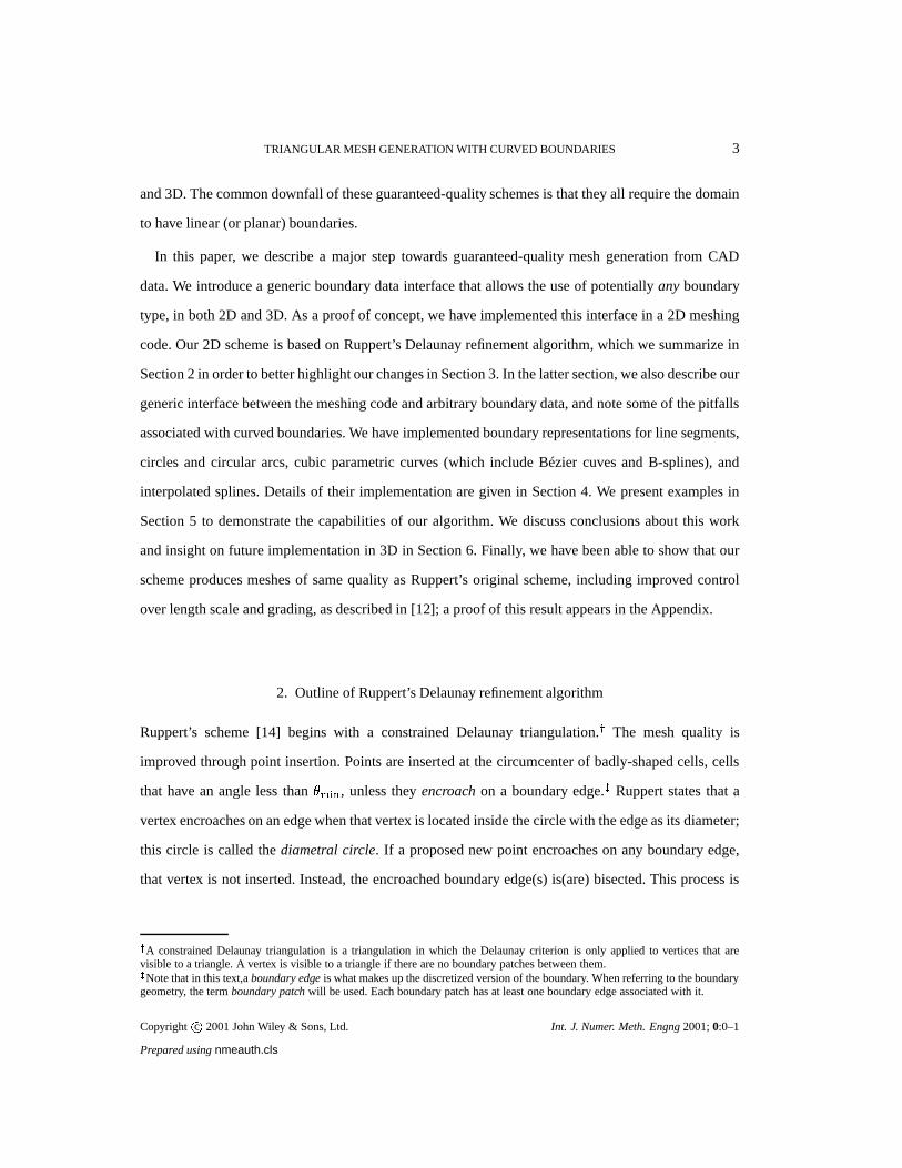
In this paper, we describe a major step towards guaranteed-quality mesh generation from CAD
data. We introduce a generic boundary data interface that allows the use of potentially any boundary
type, in both 2D and 3D. As a proof of concept, we have implemented this interface in a 2D meshing
code. Our 2D scheme is based on Ruppert’s Delaunay refinement algorithm, which we summarize in
Section 2 in order to better highlight our changes in Section 3. In the latter section, we also describe our
generic interface between the meshing code and arbitrary boundary data, and note some of the pitfalls
associated with curved boundaries. We have implemented boundary representations for line segments,
circles and circular arcs, cubic parametric curves (which include Bézier cuves and B-splines), and
interpolated splines. Details of their implementation are given in Section 4. We present examples in
Section 5 to demonstrate the capabilities of our algorithm. We discuss conclusions about this work
and insight on future implementation in 3D in Section 6. Finally, we have been able to show that our
scheme produces meshes of same quality as Ruppert’s original scheme, including improved control
over length scale and grading, as described in [12]; a proof of this result appears in the Appendix.
2. Outline of Ruppert’s Delaunay refinement algorithm
Ruppert’s scheme [14] begins with a constrained Delaunay triangulation. � The mesh quality is
improved through point insertion. Points are inserted at the circumcenter of badly-shaped cells, cells
that have an angle less than ����� � , unless they encroach on a boundary edge. � Ruppert states that a
vertex encroaches on an edge when that vertex is located inside the circle with the edge as its diameter;
this circle is called the diametral circle. If a proposed new point encroaches on any boundary edge,
that vertex is not inserted. Instead, the encroached boundary edge(s) is(are) bisected. This process is
�A constrained Delaunay triangulation is a triangulation in which the Delaunay criterion is only applied to vertices that are
visible to a triangle. A vertex is visible to a triangle if there are no boundary patches between them.Note that in this text,a boundary edge is what makes up the discretized version of the boundary. When referring to the boundary
geometry, the term boundary patch will be used. Each boundary patch has at least one boundary edge associated with it.
Copyright c�
2001 John Wiley & Sons, Ltd. Int. J. Numer. Meth. Engng 2001; 0:0–1
Prepared using nmeauth.cls

4 C. BOIVIN AND C. OLLIVIER-GOOCH
repeated until all cells are well-shaped. Ruppert was able to show that this algorithm always terminates,
and results in a mesh with minimum angle � ��� ��� �������.
Shewchuk [16] showed that a value of � ��� � of���� �
is possible if diametral lenses rather than
diametral circles are used to determine if there is encroachment. The difference between the diametral
circle and diametral lens is shown in Figure 1. In this variant of the algorithm, interior vertices lying
inside the diametral circle of a boundary edge are deleted when that edge is split. The bound on � ��� �
is not tight; in practice, � ��� � can be set to � �� and the algorithm will still terminate.
2.1. Initial discretization
Ruppert’s algorithm can be started either with a Delaunay triangulation or a constrained Delaunay
triangulation. The latter does not pose a problem because Ruppert’s original encroachment rule
guarantees that no vertex will be inserted outside a boundary edge. � A Delaunay triangulation
containing all the boundary points inside a larger bounding box is first created. Boundary edges are
recovered next using the technique described in Section 2.2. The triangles lying outside the domain are
then removed, leaving a constrained Delaunay triangulation.
The algorithm cannot be started with just any constrained Delaunay triangulation, however. No
boundary edges in the initial triangulation should be encroached on. Encroached boundary edges are
therefore split until they are not encroached upon anymore, as an initialization step. This is done by
evaluating the angle opposite the edge. If the angle is obtuse, the vertex at that corner encroaches on
the boundary edge and the edge should be split. This way, only the encroachment caused by vertices
visible to the boundary edge will be corrected, preventing unnecessary splitting of boundary edges and
introduction of artificial small features. When no more vertices encroach on boundary edges, Ruppert’s
algorithm can be started.
�The use of diametral lenses allows boundary triangles with a circumcenter outside the boundary edge to be present in the mesh.
However, no vertex will ever be inserted at this location since it encroaches on the boundary edge.
Copyright c�
2001 John Wiley & Sons, Ltd. Int. J. Numer. Meth. Engng 2001; 0:0–1
Prepared using nmeauth.cls

TRIANGULAR MESH GENERATION WITH CURVED BOUNDARIES 5
2.2. Edge recovery
The boundary edges needed for the initial discretization of the boundary are recovered through
swapping. It is always possible to recover all the edges without having to insert new points in the
domain. Once all the boundary edges have been recovered, the boundary representation is exact.
2.3. Point insertion
We insert points into the mesh by using the Delaunay insertion method of Watson [17]. We list all cells
that contain the new vertex in their circumcircle. These cells are then removed from the mesh, and the
faces of the resulting hull are connected with the newly inserted point. This insertion method preserves
the Delaunay nature of the mesh; no swapping is needed after the insertion. If a boundary edge is part
of the hull, a check is made to ensure that the new vertex will not encroach on it. If it does, the point is
not inserted. Vertices lying inside the diametral circle of the edge are removed, and the boundary edge
is split at its geometric midpoint. We use Watson insertion for this split as well.
2.4. Length scale modifications
In previous work [12], we describe how to modify Ruppert’s scheme to control cell size and grading.
The modification defines a geometric length scale based on the local feature size. The local feature size
was used by Ruppert to prove termination of the original algorithm, and is defined as the radius of the
smallest circle centered at a point that touches two disjoint parts of the domain boundary. We defined
the length scale ��� in terms of the local feature size � ��� as:
����� ��������� � � ��������� � �����neighbors ��� ����! #"��%$'&(*)�+ #"-, + ) . (1)
where both�
and(
are constants / & , and points 0" are neighbors to point . The first constant,�, controls the ratio of input feature size to final mesh boundary edge length, with finer boundary
discretization for larger values of�
. The other constant,(
, is used to control how rapidly the cell size
can change with distance. This is an explicit imitation and generalization of the grading properties of
the local feature size. A larger value of(
results in slower increase in cell size over the same distance.
Copyright c�
2001 John Wiley & Sons, Ltd. Int. J. Numer. Meth. Engng 2001; 0:0–1
Prepared using nmeauth.cls

6 C. BOIVIN AND C. OLLIVIER-GOOCH
The value of ��� is stored at every vertex location.
Ruppert’s scheme was modified to also split cells that are too large according to the definition of
length scale in Equation 1. A cell is considered too large whenever the ratio of its circumradius to the
average ��� of its vertices is greater than � �� .
Implementation details, such as how the � �#� is computed, as well as a proof that the modified
algorithm terminates with quality bounds comparable to Ruppert’s are provided in [12].
2.5. Small angles in the domain
Small angles in the domain definition are problematic because they can lead to infinite recursion when
trying to fix the encroachment of a boundary edge. Ruppert [14] identified this pitfall and suggested the
use of concentric circular shells around small angles to prevent it. Figure 2 illustrates this. Boundary
edges that are connected to a small angle vertex are split at the intersection with circular shells centered
at the vertex — not at the midpoint of the edge. This has the effect of creating protective layers around
the small angle boundary vertex, preventing encroachment. This technique was also used in the present
research.
3. Generic boundary interface
To enable meshing from general curved boundaries, we need a framework in which the mesh generation
code makes no assumptions about the underlying geometry of boundary patches [15]. This implies a
generic interface between mesher and geometry, in which the mesher only needs the results of several
geometric queries. This is illustrated in Figure 3.
Whenever the mesh generation algorithm needs information about the boundary, a “question” is
passed on to the proper type of boundary patch. Each boundary patch type knows how to answer all of
these questions, and the answer is then passed back to the algorithm. This provides a transparent access
to potentially any type of boundary patch. Using object-oriented programming, this generic interface
can be implemented by using a common base class for all boundary data, with implementation of
specific geometric queries in derived boundary data classes.
Copyright c�
2001 John Wiley & Sons, Ltd. Int. J. Numer. Meth. Engng 2001; 0:0–1
Prepared using nmeauth.cls

TRIANGULAR MESH GENERATION WITH CURVED BOUNDARIES 7
The information required for the successful implementation of Ruppert’s algorithm — curve
midpoint, curvature, and original discretization information — is described in Sections 3.2 to 3.6.
The other questions are needed to determine the appropriate mesh length scale ��� . This is the reason
they are implemented; they will not be discussed any further in this text. See [12] for more information.
So far, classes for lines, circles, arcs, cubic parametric curves, and interpolated splines have been
written. New types of boundary patches can be added by providing the proper “answers” for the given
boundary patch.
3.1. Total variation of the tangent angle
Since the meshing code must be able to work with curved as well as linear patches, a new way of
determining where splits happen along a boundary patch is necessary. We first make the observation
that patches with little orientation change need few, long edges for accurate geometric representation.
Linear patches have no orientation change; they can be represented accurately with just one edge.
In contrast, regions of a curve with a large change in orientation require a greater number of shorter
edges. We must also make sure that small amplitude sine-like curves are discretized appropriately. This
suggests we should use the total variation of the tangent angle of a curve to determine where to split a
boundary patch.
The total variation ��� � � � is defined in the following way:
��� � � � � � )�� � ) (2)
By using the following definition of curvature:
� � � �������� �� � ����
it is possible to obtain an another form for Equation 2:
��� � � ��� � ) � � ) � � ) � � �0� )� �Copyright c
�2001 John Wiley & Sons, Ltd. Int. J. Numer. Meth. Engng 2001; 0:0–1
Prepared using nmeauth.cls

8 C. BOIVIN AND C. OLLIVIER-GOOCH
The total variation can therefore also be expressed as the integral of the non-negative curvature
along the arclength. Note that there is no need to compute the integral; one simply needs to compare
the orientation of the curve’s tangent vector at carefully chosen points along the boundary patches to
get the exact value of ��� � � � . More details are given for each type of boundary patches in Section 4.
3.2. Initial discretization
To obtain the initial Delaunay triangulation, each boundary patch must be initially discretized in
some way. Since the exact shape of the boundary is only known by the boundary patches, the initial
discretization of the corresponding curve must be computed by the patches themselves. At this point
in the meshing process, we represent curves with as few edges as possible in order not to introduce
artificial small features in the mesh. However, we must make sure that a valid and exact representation
of the domain will be obtained and that the rules regarding the location of points inside the diametral
lenses are also followed.
An arbitrary discretization of a spline curve is shown in Figure 4. We wish to triangulate outside
(above) the curve. Ruppert’s scheme guarantees that no vertex will be inserted inside (below) the
boundary edges. We also want to make sure that no vertex will be inserted in the regions inside the
curve but outside of the boundary edges (the shaded area in Figure 4). This is to prevent an invalid
discretization, as the vertex inserted in the shaded area would ultimately lie outside the domain once
the boundary is well-resolved.
The protection of this area can be achieved by making sure that the diametral lenses of the boundary
edges completely include the curve boundary. Since points are never inserted inside the diametral
lenses, this will protect the shaded region from point insertion. It is easy to calculate the total variation
in orientation a curve can have to remain inside the diametral lens of a corresponding discretized edge.
The diametral lens, as seen in Figure 5 makes a � � angle with edge ab. A curve passing through
both points a and b can make an angle of � � ,�� with the horizontal at point a and an angle of ,�� with
the horizontal at point b and still be completely inside the diametral lens. This results in a ��� � � � of
��� � . This is the maximum total variation in orientation a curve can have in order to pass through both
points a and b, and still remain inside the diametral lens. A bigger change can potentially put the curve
Copyright c�
2001 John Wiley & Sons, Ltd. Int. J. Numer. Meth. Engng 2001; 0:0–1
Prepared using nmeauth.cls

TRIANGULAR MESH GENERATION WITH CURVED BOUNDARIES 9
outside of the lens. A valid initial discretization scheme must therefore limit the length of edges so that
the ��� � � � of the curve over them does not exceed ��� � , i.e. ��� � � � ����� � ��� � . The diametral lenses
of all the boundary edges will then entirely contain their corresponding boundary patch, therefore not
allowing any vertices to be inserted in the shaded areas of Figure 4.
In addition, whenever a new boundary point is inserted, one must make sure that the two newly
created boundary edges will have diametral lenses that are point-free to prevent insertion outside the
domain. In Shewchuk’s modification to Ruppert’s scheme, all points in a boundary edge’s diametral
circle are deleted before the edge is split; we do the same in our scheme.
As can be seen from Figure 6, a curve with uniform curvature will intersect the edge with angles
of � �� at each endpoint. Knowing that the diametral circle of the original boundary edge is always
point-free, it is easy to see that the diametral lenses of new boundary edges coming from this curve
will also be point-free. The diametral lenses will always be contained within the diametral circle. Such
a statement is not true, however, for non-uniform curvature patches. For such curves, the incident angle
with the boundary edge can be arbitrarily close to � �� . This could result in a diametral lens that is not
entirely contained within the diametral circle whenever that curve needs to be further split, as illustrated
in Figure 7. The area with a white background is point-free whereas the area with a shaded background
might contain points. It can be seen that part of the new diametral lens lies in the shaded area.
This pitfall is avoided by limiting ��� � � � ����� along a boundary edge to ��� � for boundary patches
with non-uniform curvature. While this leads to twice as many boundary edges needed for curves
with non-uniform curvature compared to uniform-curvature patches, this representation is still coarse
enough not to introduce any artifical small feature in the mesh. More details are given in Section 3.5.
The general scheme for the original discretization of the boundary patches is therefore to first
calculate the orientation change over the complete patch. The number of edges is then found by
ensuring that each edge, when split at equal intervals of ��� � � � , will cover less than the maximum
allowed for a given type of boundary patch (i.e ��� � for patches with uniform curvature, ��� � for patches
with non-uniform curvature). The following formula can be used for the number of edges:
Copyright c�
2001 John Wiley & Sons, Ltd. Int. J. Numer. Meth. Engng 2001; 0:0–1
Prepared using nmeauth.cls

10 C. BOIVIN AND C. OLLIVIER-GOOCH
��� � � ��� � � ���� � � � ������� (3)
The new vertices will be located where the orientation change from the previous vertex is:
��� � � � � � ��� � � ����3.3. Edge recovery
Due to the very coarse representation of the boundary patches during edge recovery, some precautions
must be taken in order to get a valid initial constrained Delaunay triangulation. The edge recovery
process must be modified since simple recovery through swapping will fail in some cases. Two
categories of such cases have been found. A description of these and an overview of the edge recovery
strategy used to obtain valid initial triangulations follow.
3.3.1. Crossing of initial discretization edges The initial discretization suggested by the boundary
patches may result in an invalid overall discretization, because the edges that need to be recovered
cross each other. Such a case is shown in Figure 8, which presents a square inside a circle, including
the initial discretization of the circle. The top and bottom edges of the circle’s discretization cross the
edges of the square. Clearly, not all edges in this initial discretization can be recovered simultaneously.
Detecting such cases in advance can be computationally expensive. Instead, we take advantage of the
fact that it is also possible to recover edges through vertex insertion, a process referred to as stitching.
If an edge is not present in the mesh, a vertex is inserted at the midpoint of its corresponding patch.
If any of the two resulting edges is still absent from the mesh, then it is once again split. This method
is guaranteed to recover all the edges since a vertex is always connected to its nearest neighbors in a
Delaunay triangulation [16]. The spacing between the vertices of a boundary patch will eventually be
small enough that the corresponding boundary edges will have to be present in the triangulation.
However, when forming a constrained Delaunay triangulation, blindly inserting vertices for a
missing edge can lead to a very large number of unnecessary vertices. Consider for example the domain
presented in Figure 9. Since vertex a is so close to edge bc, many vertices would need to be inserted on
Copyright c�
2001 John Wiley & Sons, Ltd. Int. J. Numer. Meth. Engng 2001; 0:0–1
Prepared using nmeauth.cls

TRIANGULAR MESH GENERATION WITH CURVED BOUNDARIES 11
edge bc in order to recover the edge. This would lead to an artifical small feature in the triangulation.
Obviously, this is to be avoided.
We balance these competing requirements by inserting vertices only when swapping has failed. We
first go through the list of edges and recover them through swapping. Since the edges are not locked
once they are recovered, it is possible that the recovery of one edge makes a previously recovered
edge disappear. Any edge associated with a curved patch that is still missing after this step will have
a vertex inserted at its corresponding midpoint. Recovery of edges associated with linear patches is
always done through swapping. By following this method, only the necessary vertices are inserted and
no artifical small feature is introduced in the constrained triangulation. The initial discretization for the
case described in Figure 8 is shown in Figure 10.
3.3.2. Boundary edges located in wrong region It is also possible that, due to the rather coarse
discretization of curved boundary patches, entire boundary edges will be located in the wrong region.
This problem has the same source as the previous one, except that in this case, the boundary edges do
not overlap. In such a case, all boundary edges can be recovered, but the initial discretization is still
invalid.
Figure 11 illustrates this. The small square is located to the right of the boundary edge ab. However,
it is located to the left of boundary patch ab. In this case, the small square would be located outside the
triangulation, which can not be allowed.
The easy way to detect this case is to make sure that a vertex connected to edge ab on the left side
is also on the left side of the corresponding curved boundary patch. If the two sides are different, then
edge ��
is split. This check must be done for both vertices located opposite each edge in the mesh
associated with non-linear boundary patches.
As a summary, Figure 12 shows a diagram of the procedure to follow for edges to be recovered. The
process is over once all the edges are recovered in one pass.
Copyright c�
2001 John Wiley & Sons, Ltd. Int. J. Numer. Meth. Engng 2001; 0:0–1
Prepared using nmeauth.cls

12 C. BOIVIN AND C. OLLIVIER-GOOCH
3.4. Point insertion
Point insertion in the mesh, as well as on the boundary, is still done using Watson’s method. However,
curved boundaries modify the way that boundary edges are split. Instead of splitting at the average
location of the edge’s vertices, the location of the new boundary vertex is determined by the boundary
patch itself. The “midpoint” between two vertices is now found using the total variation of the tangent
angle. The general technique is to first find the total variation of the tangent angle between the boundary
edge’s vertices � and�. The midpoint � will be located at the point on the curve where ��� � � � between
� and � and between � and�
is equal. This ensures that the new point is always located on the boundary
and that regions of the curve with higher curvature will be discretized with more edges.
If the curvature over a given boundary edge is (almost) zero, the orientation change is negligible. In
these cases, the split is made according to arclength. This ensures linear patches are split in the same
fashion as before, and it also handles curves that have particularly flat regions.
The fact that the midpoints are no longer always located on the boundary edge being split can lead
to problems. In some cases, boundary edges may cross nearby boundary patches. An example of such
a case is shown in Figure 13. If the first edge of the bottom arc���
happens to be split before the first
edge of the top arc ��� , point � will be inserted outside the domain, which can not be allowed.
The strategy to fix this problem uses the fact that the boundary vertex � inserted to split the bottom
arc���
will not only lie behind edge ��� but will also encroach on ��� since arc ��� is completely
included in the diametral lens of edge ��� . This fact ensures that we can always find the edge ��� to
test whether the new vertex � lies behind it. When the new vertex lies outside the domain and some
edge ��� separates the vertex from the edge���
that it is supposed to split, then we must first split
��� . In other situations, we split���
first; this prevents infinite recursion.
Even with this change in point placement when splitting boundary edges, we are still able to
construct a proof showing that the modified algorithm will terminate with bounds on mesh quality
similar to Ruppert’s original scheme. See the Appendix for the complete details of the proof.
Copyright c�
2001 John Wiley & Sons, Ltd. Int. J. Numer. Meth. Engng 2001; 0:0–1
Prepared using nmeauth.cls

TRIANGULAR MESH GENERATION WITH CURVED BOUNDARIES 13
3.5. Length scale modifications
Whenever a boundary edge is split, the length scale ��� ���� for the new boundary vertex needs to be
computed using Equation 1. For this, we need the local feature size � �#� � � at the new point to take
into account the curvature of the boundary. We define the local feature size for curved boundaries, � �����to be:
� �����#� ��������� � � ���� � � ��� �� � � (4)
where � �� ��� �� ����� � is the radius of curvature at point . The radius of curvature therefore provides
a ceiling on the value of the local feature size on the boundary. By using the radius of curvature, there
will be an equal number of points per radian on the curve as per gap between objects. For curves with
uniform curvature, the edge length from initial discretization and the radius of curvature are equal.
For non-uniform curves, with a ��� � � � ����� of ��� � , the edge lengths will be twice as small. This will
lead to more points on the curved boundary, as needed. This factor of two will not lead to artificial
small features since the ��� at that point might be determined by neighbor vertices, not by � �����#� � .Furthermore, we can only prove that the edge lengths will be within a factor � ��� $ & � ( � of their ideal
length. See the Appendix for details on the proof.
3.6. Small angles in the domain
The concentric circular shells method described in Section 2.5 can also be used to prevent infinite
insertion around small angles created between two curved boundaries. However, one must make sure
that the split points are located using geometric distance from the small angle vertex. If total variation
of the orientation is used instead of geometric distance, infinite encroachment is still possible, as
illustrated in Figure 14a. Vertices a and b were first created, perhaps as part of the initial discretization.
Since � � �� is obtuse, vertex � was inserted to fix encroachment on edge � � . However, � encroaches
on � � � so it too must be split, using point � . However, � ��� � is still obtuse, so edge � � should be split,
and so should ��� � etc. Such a problem does not appear when geometric distance from vertex c is used
instead of orientation change, as can be seen from Figure 14b.
Copyright c�
2001 John Wiley & Sons, Ltd. Int. J. Numer. Meth. Engng 2001; 0:0–1
Prepared using nmeauth.cls

14 C. BOIVIN AND C. OLLIVIER-GOOCH
4. Implementation details
The evaluation of the total variation of orientation over any type of boundary patch is the cornerstone
of both the initial discretization and the midpoint routines. As was mentioned in Section 3.1, there is
no need to actually compute the integral; one only needs to take the difference in orientation between
two points over which the change in orientation of the curve is monotone, i.e. it is either non-varying,
or is strictly increasing or decreasing. The details on how to find these particular points are given in the
following sections.
4.1. Linear patches
The implementation of this type of patch is straightforward. The orientation change over any linear
patch is simply zero. Consequently, edges are split at the geometric midpoint of the edge.
Likewise, the initial discretization of a linear patch is trivial: only one edge is needed. The two
endpoints of the edge are inserted in the mesh, and the edge between these endpoints is marked for
recovery. No other vertices need to be inserted.
4.2. Circles and circular arc patches
The total variation of orientation for these patches is easy to obtain since the curvature of a circular arc
(or circle) is a constant & � � . In order to exactly evaluate Equation 2, one only needs to use the second
form of the orientation change integral and find the total arclength of the arc, a trivial computation
given that the endpoints of the arc are known.
The midpoint between two vertices is calculated using the total variation of the orientation. However,
since the curvature is constant, this is equivalent to splitting on arclength alone, and is simple to
implement. The original discretization demands a bit more caution. First, the number of edges needed
to discretize the arc is found using Equation 3. The value of ��� � � � ����� for patches with uniform
curvature is ��� � . The endpoints, as well as the extra vertices needed to define the proper number of
edges are inserted in the mesh and the� �
edges are marked for recovery. Note that for full circles,
there are no endpoints, and� �
is always six.
Copyright c�
2001 John Wiley & Sons, Ltd. Int. J. Numer. Meth. Engng 2001; 0:0–1
Prepared using nmeauth.cls

TRIANGULAR MESH GENERATION WITH CURVED BOUNDARIES 15
4.3. Cubic parametric curves
Cubic parametric curves are internally defined by two cubic parametric equations � � � � and � � � � , with�
varying between 0 and 1. Such definition allows the representation of cubic Bézier curves, cubic
B-splines and cubic interpolated splines (see section 4.4 for details on splines). In order to compute
��� � � � , we need to find the “critical” values of�
between which the orientation of the curve must be
monotone. This way, it is possible to simply take the difference in the orientation of the curve at these
points to find the total orientation change for the curve. Furthermore, if we are careful to take points on
the curve that only allow a maximum change of ��� � between them, we eliminate the need to determine
if the curve changed orientation by a value of � or a value of� � ,�� �
To achieve this, we select the minima and the maxima of both � � � � and � � � � as critical points.
This limits ��� � � � between two critical points to be smaller than ��� � . There are as many as two such
points for each cubic equation. The inflexion point for each cubic equation is also chosen as a critical
point. Finally, the orientation of a cubic parametric curve might reach a maximum or a minimum at
the locations where the curvature is zero. These locations are found using the following definition of
curvature:
� � )���� )� �
where � � )�� ) . Clearly, the curvature will go to zero whenever )����� ) does. From this, we
get as many as two more critical points on the curve, since ���� � �simplifies to a quadratic
equation for cubic parametric curves. In summary, we potentially have eight critical values of�
for a
2-D cubic parametric curve: four maxima/minima, two inflexion points, and two zero-curvature points.
By ordering these and the endpoints, and then taking the difference in the orientation of the curve
between consecutive values, we obtain the exact answer to Equation 2. An example of a Bézier curve
with eight critical points in shown in Figure 15. Two critical points are very close to each other on the
left part of the curve.
These critical points are stored, and are used to quickly find the location of a midpoint. The location
Copyright c�
2001 John Wiley & Sons, Ltd. Int. J. Numer. Meth. Engng 2001; 0:0–1
Prepared using nmeauth.cls

16 C. BOIVIN AND C. OLLIVIER-GOOCH
is isolated between two of these critical values (or one of them and an endpoint). Since the curve is
monotone between two of these points, it is then possible to use interpolation techniques to find the
exact location of the midpoint.
The initial discretization of a parametric curve follows the generic procedure outlined earlier. In this
case, ��� � � � ����� � ��� � . The endpoints, as well as the new discretization vertices, are inserted in the
mesh, and the� �
edges are marked for recovery.
4.3.1. Tangent vector may be null It is possible to obtain a cubic parametric curve where both
components of the tangent vector are zero. This prevents us from using the tangent vector (or the normal
vector, which depends on the same data) to determine the orientation of the curve at that particular
point. The orientation is usually found using:
� � � � ������� � � � � ��� � � �� � � � � .The signs of ���� � � and ��� � � � are used to determine the quadrant of � � � � . The tangent vector is null
whenever both ���� � � and ��� � � � are zero for some� � �� . This makes the ratio of the two indeterminate:
� ��� ��� �� ���!� � �� � � � � ���
By using L’Hospital’s rule, the limit becomes:
� ��� ��� � � � � � � �� � � � � �We keep using L’Hospital’s rule until a finite value for the ratio is found. We can then use this finite
value to determine the orientation at� � �� , i.e.
� � � � ������� � � � � ��� � � � �� � � � �� � .However, in order to determine the right quadrant for � � � � � we must still use the signs of ��� � � � and
��� � � � as they approach��
. This can be done by evaluating them with a value of�
close to��
and still
Copyright c�
2001 John Wiley & Sons, Ltd. Int. J. Numer. Meth. Engng 2001; 0:0–1
Prepared using nmeauth.cls

TRIANGULAR MESH GENERATION WITH CURVED BOUNDARIES 17
within�
and & .4.4. Cubic interpolated splines
An interpolated spline is a collection of � , & cubic parametric curves, where � is the number of
points to be interpolated. As such, its total variation of the tangent angle is just the sum of the total
variations of its cubic curves. In the present research, the interpolated splines are created with “no-
moment” boundary conditions, i.e. both � � ��� � � and ��� � � � � are set to zero at the endpoints. Note that the
interpolation points are not necessarily inserted in the mesh – they only define the shape of the curve.
The list of critical points for an interpolated spline includes all the critical points of its cubic curves as
well as their endpoints. The midpoint is found using the same technique as described in Section 4.3,
i.e. interpolation techniques are used once the two surrounding critical points are known.
Initial discretization of an interpolated spline is a bit more complicated, as boundary edges will now
more than likely span more than one parametric cubic curve. However, the overall process is the same
as for cubic parametric curves, with ��� � � � ����� also ��� � .
5. Results
Figure 16 details the different steps involved in generating a mesh with the generic boundary interface.
The domain to be discretized, shown in Figure 16a, consists of four linear patches, one Bézier curve (in
the lower-right quadrant), and one circle. The interior of the circle is considered hollow in this case and
will not be triangulated. Figure 16b shows the result of the initial discretization. The domain, defined
by the cells, was shaded in order to provide a better idea of its shape. The circle was discretized using
6 edges. The Bézier curve, spanning� �
, was discretized with three edges. This is in accordance with
the procedure described in Section 4.We can clearly observe the non-uniform distribution of the extra
vertices due to splitting according to orientation change. We can also see that a boundary edge in the
lower right quadrant crosses another boundary patch, a problem that was discussed in Section 3.4.
Even though the mesh in Figure 16b is a valid constrained Delaunay triangulation, encroached
boundary edges must be split before Ruppert’s algorithm can be started, as described in Section 2.1.
Copyright c�
2001 John Wiley & Sons, Ltd. Int. J. Numer. Meth. Engng 2001; 0:0–1
Prepared using nmeauth.cls

18 C. BOIVIN AND C. OLLIVIER-GOOCH
Figure 16c is the result of the encroachment fix step, and this is the triangulation that Ruppert’s
algorithm is started with. Note that the circle is now discretized much more precisely in its lower-right
quadrant than elsewhere because of its proximity to the Bézier curve.
We can see the final result of Ruppert’s algorithm in Figure 16d. All of the angles in this mesh, and
the following ones, are equal to or larger than � �� . To demonstrate how the generic boundaries adapt
to a change in required resolution, we have generated meshes with two and four times the resolution of
the mesh in Figure 16d. These are shown in Figures 16e and 16f, respectively.
Figures 17 and 18 show that the algorithm can easily handle complex geometries with generic
boundaries. They were both created using� � ( ��� . In order to demonstrate more practical uses,
we have also included the mesh of the region surrounding a 4-element airfoil, shown in Figure 19. The
boundary geometry is defined by a circle and four interpolated splines. This relatively coarse mesh was
created using� � ( � & for clarity. The immediate surroundings of the airfoil are shown magnified
in Figure 20, with 20a detailing the state of the mesh after initial discretization, and 20b the final result
from Figure 19.
Table I summarizes the quality of the three previous meshes. The size and grading parameters used,
the minimum and maximum angle in the mesh, as well as the ratio of the actual edge length to the
“theoretical” edge length (from the average of the ��� at its vertices) are listed. These meshes were all
generated with an imposed minimum angle bound of � �� . With higher values of�
and(
, the major
constraint is the cell size, not its shape. This explains why the angle bounds as well as the edge length
ratios are better for these cases. For case with lower values of�
and(
, the angle bound is harder
to reach than the size constraint. This results in smaller cells in some regions, which affects the edge
length ratios.
The use of the generic boundary interface did have a small impact on the time required to insert
points on the boundary. The boundary point insertion routines, which include the calls to determine
the location of the new midpoint, take about 5% longer than before, on average. However, considering
that, on a typical mesh, the time spent on boundary insertion accounts for less than 1% of the total
time, the overall impact on performance is negligible.
Copyright c�
2001 John Wiley & Sons, Ltd. Int. J. Numer. Meth. Engng 2001; 0:0–1
Prepared using nmeauth.cls

TRIANGULAR MESH GENERATION WITH CURVED BOUNDARIES 19
6. Conclusions
We have presented a new framework allowing the use of curved boundaries with a guaranteed-quality
Delaunay refinement algorithm. The boundary data has been separated from the meshing algorithm,
removing all assumptions about the shape of the boundary from the meshing code.
The use of curved boundaries demanded a new way of splitting boundary edges, to ensure regions
with higher curvature were discretized with a greater number of edges. The midpoints are now
computed using the total variation of the tangent angle, ��� � � � . Whenever ��� � � � is negligible over a
given boundary edge, the arclength is used to compute the midpoint.
The introduction of curved boundaries also demanded a new initial discretization strategy. Curved
patches are first discretized with as few segments as possible. The minimum number of segments
required is determined by the total variation of the tangent angle of the patch. We make sure that
the curved patch is always protected by the diametral lenses of its boundary edges. We found some
recovery problems associated with this rather coarse initial representation of the boundary. A new
strategy for edge recovery was developed and presented in this document.
Several patch types have been implemented and tested successfully. New boundary types can be
added to the generic boundary interface by implementing responses for all the generic queries used by
the meshing algorithm.
Finally, we showed examples demonstrating the successful use of curved boundary patches. These
meshes all showed excellent quality, with a minimum angle exceeding � � in all of them. Their
resolution and grading were easily controlled using parameters�
and(
. We also also found that
the generic boundary interface had a negligible impact on the time required to mesh a domain.
6.1. Extension to three dimensions
We are currently beginning work to extend support for meshing from curved boundaries to three
dimensions. As in two dimensions, we will isolate the meshing code from the geometry from a generic
interface. Among other things, this will allow use of various CAD database formats for the cost of
writing wrapper functions to query those databases. As usual, we expect more problems to crop up in
Copyright c�
2001 John Wiley & Sons, Ltd. Int. J. Numer. Meth. Engng 2001; 0:0–1
Prepared using nmeauth.cls

20 C. BOIVIN AND C. OLLIVIER-GOOCH
three dimensions, especially in the area of initial discretization, both of the surface and the volume.
Initial discretization will probably be the pacing item for this work.
REFERENCES
1. I. Babuska and A. Aziz. On the angle condition in the finite element method. 13:214–226, 1976.
2. L. Paul Chew. Guaranteed-quality triangular meshes. Technical Report TR-89-983, Dept. of Computer Science, Cornell
University, 1989.
3. L. Paul Chew. Guaranteed-quality mesh generation for curved surfaces. In Proceedings of the Ninth Annual Symposium
on Computational Geometry, pages 274–280. Association for Computing Machinery, May 1993.
4. Saikat Dey, Robert M. O’Bara, and Mark S. Shepard. Curvilinear mesh generation in 3D. In Proceedings of the Eighth
International Meshing Roundtable, pages 407–417, October 1999.
5. H. Edelsbrunner and D. Guoy. Sink-insertion for mesh improvement. In Proceedings of the 17th ACM Symposium on
Computational Geometry, pages 115–123, June 2001.
6. Lori A. Freitag and Carl F. Ollivier-Gooch. A cost/benefit analysis of simplicial mesh improvement techniques as measured
by solution efficiency. International Journal for Computational Geometry, August 2000.
7. I. Fried. Condition of finite element matrices generated from nonuniform meshes. AIAA Journal, 10:219–221, 1972.
8. Patrick Laug, Houman Borouchaki, and Paul-Louis George. Maillage de courbes gouverné par une carte de métriques.
Technical Report RR-2818, INRIA, 1996.
9. D.J. Mavriplis and S. Pirzadeh. Large-scale parallel unstructured mesh computations for 3D high-lift analysis. Journal of
Aircraft, 36(6), 1999.
10. Fotis Mavriplis. CFD in aerospace in the new millenium. Canadian Aeronautics and Space Journal, 46(4):167–176,
December 2000.
11. Scott A. Mitchell and Stephen A. Vavasis. Quality mesh generation in three dimensions. In Proceedings of the ACM
Computational Geometry Conference, pages 212–221, 1992. Also appeared as Cornell C.S. TR 92-1267.
12. Carl F. Ollivier-Gooch and Charles Boivin. Guaranteed-quality simplicial mesh generation with cell size and grading
control. Engineering with Computers, 17:269–286, 2001.
13. M.-C. Rivara. New longest-edge algorithms for the refinemetn and/or improvement of unstructured triangulations.
International Journal for Numerical Methods, 40:3313–3324, 1997.
14. Jim Ruppert. A Delaunay refinement algorithm for quality 2-dimensional mesh generation. Journal of Algorithms, 18:548–
585, 1995.
15. A. Sheffer and A. Ungor. Efficient adaptive meshing of parametric models. In Proceedings of the 6th ACM Symposium on
Solid Modeling and Applications, pages 59–70, June 2001.
16. Jonathan R. Shewchuk. Delaunay Refinement Mesh Generation. PhD thesis, School of Computer Science, Carnegie
Mellon University, May 1997.
Copyright c�
2001 John Wiley & Sons, Ltd. Int. J. Numer. Meth. Engng 2001; 0:0–1
Prepared using nmeauth.cls

TRIANGULAR MESH GENERATION WITH CURVED BOUNDARIES 21
17. David F. Watson. Computing the � -dimensional Delaunay tessellation with application to Voronoi polytopes. Computer
Journal, 24(2):167–172, 1981.
APPENDIX
II. Proof of Mesh Quality in Two Dimensions
The proof presented in this appendix follows the same approach used in previous research [12]. We
assume that boundary edges are protected by diametral lenses and that input angles are greater than
� � , to prevent adjacent edges from encroaching on each other. We will be able to show the same
bounds for curved boundaries that we previously demonstrated for straight boundaries.
We will now prove the following lemma, which will, among other results, establish an angle bound
for finite cell size and hence for algorithm termination. This lemma is deliberately stated in language
as similar as possible to Ruppert’s Lemma 2, even to exact quotation of much of the phrasing, although
details of the proof and the derived constants differ.
Lemma 1. (After Ruppert [14]) For fixed constants ��� , ��� and � � , determined below, the
following statements hold:
1. At initialization, for each input vertex , the distance to its nearest neighbor vertex is at least
� �#� �%� ���� ��� ������� .2. When a point is chosen as the circumcenter of an overly-large triangle, the distance to the
nearest vertex is at least ��� �� � � �� . ( may be added to the triangulation, or may be rejected
because it encroaches upon some segment.)
3. When a point is chosen as the circumcenter of a skinny triangle, the distance to the nearest
vertex is at least ��� � � � � � . (Again, may be added to the triangulation, or may be rejected
because it encroaches upon some segment.)
4. When a vertex is added as the midpoint of a split segment, the distance to its nearest neighbor
vertex is at least ��� � � � � � .
Proof.
Copyright c�
2001 John Wiley & Sons, Ltd. Int. J. Numer. Meth. Engng 2001; 0:0–1
Prepared using nmeauth.cls

22 C. BOIVIN AND C. OLLIVIER-GOOCH
Case 1. Statement 1 of Lemma 1 is true by the definition of the length scale ��� from the local
feature size � �#� � , provided only that the constant�
in Equation 1 is / & .Having established the truth of Lemma 1 for the initial mesh, we will proceed by induction to prove
that it must be true for all meshes generated by the algorithm. As such, we will assume that Lemma 1
holds for all points in the mesh and determine the bounds on � � , � � , � � , and(
that are required for
Lemma 1 to hold for newly inserted points.
Case 2. We consider first the case of insertion to split a large triangle, as shown in Figure 21. By
definition, the circumradius of�
�� � is larger than � �� times the average of the length scales at its
vertices. The distance from to the nearest point is the circumradius of�
�� � , or
� / � �� ���� � � $ ��� � � �-$ ���� � �� (5)
We can bound the length scale at in terms of this same average using Equation 1:
��������� ���� � �-$ �(��������� ���� � �%$ �(��������� ���� �#�-$ �(��������� ���� � �%$ ��� � � �%$ ���� �#�
� $ �( (6)��� � � �-$ ���� � �%$ ���� �#�� / ����� � , �(
Combining inequalities 5 and 6, we get
� / � � �������� , � � �� (� / �������� � $ �� (7)
This inequality places a lower bound on point spacing for points inserted to split large triangles, and
Copyright c�
2001 John Wiley & Sons, Ltd. Int. J. Numer. Meth. Engng 2001; 0:0–1
Prepared using nmeauth.cls

TRIANGULAR MESH GENERATION WITH CURVED BOUNDARIES 23
confirms Statement 2 of Lemma 1, for any
��� / � � $ &( (8)
The lower bound on � � becomes smaller for large values of(
, corresponding to slow change in cell
size.
Case 3. We consider next the case of insertion to split a badly shaped triangle, as illustrated in
Figure 22. Without loss of generality, we can label vertices so that � and�
are connected by the shortest
edge (of length � ��� � ), and � was inserted in the mesh after�
(or both were input vertices). The radius
of the vertex-free circle around � is � � . Four subcases for relating � � to ������� arise, depending on why
� was inserted in the mesh.
Subcase 3a. � was an input vertex. Then so was�, Statement 1 of Lemma 1 applies, and the distance
� ��� � / � � ���� � � .Subcase 3b. � was inserted to split a large triangle. The circumradius � � of that triangle is no larger
than � ��� � , because vertex�
was not inside the circumcircle. Then Statement 2 of Lemma 1
applies, and � ��� ��/ � �-/ ���� � � � � � .
Subcase 3c. � was inserted to split a badly shaped triangle. By a similar argument and using Statement
3 of Lemma 1, and � ��� � / � �-/ ���� � � � � � .
Subcase 3d. � was inserted to split an encroached boundary edge. We know that�
does not lie
inside the diametral lens of the edge � split, because otherwise�
would encroach on that edge.
Statement 4 of Lemma 1 applies, and � ��� � / � �-/ ��� � � � � � � .
If we satisfy � � / ���*� � �*/ & (which we will show is possible), then the inequality � ��� � /��� � � � � � � (subcase 3d) causes the most difficulty in satisfying Statement 3 of Lemma 1 by making
the length scale at larger than that for any other subcase.
We can relate the radius � of the circumcircle of�
�� � to its smallest angle. The angle � �0 � � � �
Copyright c�
2001 John Wiley & Sons, Ltd. Int. J. Numer. Meth. Engng 2001; 0:0–1
Prepared using nmeauth.cls

24 C. BOIVIN AND C. OLLIVIER-GOOCH
by geometry, and trigonometry gives � ��� � � � ��� ��� � . The definition of length scale gives
������� � ���� � �-$ �( � � � � ��� � $ �(� � � � � � ��� � $ �( (9)
This triangle is being split because � is less than the required angle bound � . We can strengthen
Inequality 9 by replacing � with � , and obtain
� / ��������� $ � � � � �����Lemma 1 states that, for this case, � / ������� � ��� , so we require that
� � / &( $ � � � � ����� (10)
Case 4. Now we turn our attention to the case in which vertex is added to the mesh to split a
segment � , because some vertex or triangle circumcenter lies inside the diametral lens of � . Vertex is
inserted on the patch between�
and � , not necessarily at the midpoint of edge� � .This case is illustrated
in Figure 23. There are four subcases.
Subcase 4a. � lies on a segment�, which can not share a vertex with � , because we have assumed
that input edges are separated by 60. Therefore, and � lie on non-adjacent segments, and the
length scale at is ����� � � �� )�+� , + ) . To satisfy Lemma 1 in this subcase, we therefore require
that � � / �� . Because
� / & , this inequality is always satisfied for � � / & .Subcase 4b. � is a point at the circumcenter of a large triangle � . � has of course been rejected for
insertion since it is located inside the diametral lens. The definition of the length scale then gives:
��������� ��� � � �-$ �� ) +� , + )The circumradius � � of � is smaller than the shorter of ���
+� , +� ��� and ) +� , +� ) , because � ’s
Copyright c�
2001 John Wiley & Sons, Ltd. Int. J. Numer. Meth. Engng 2001; 0:0–1
Prepared using nmeauth.cls

TRIANGULAR MESH GENERATION WITH CURVED BOUNDARIES 25
circumcircle must be point-free. The largest value of � � is obtained when � is at the apex of
the diametral lens, so � � � �� �� . Also, we know from this lemma that ��� � � � � ��� � � � .
Furthermore, the largest value of ) +� , + ) places � and at opposite ends of edge� � , so
)�+� , + ) � � � . The length scale at now becomes:
��������� � � ����$ ���
� ��
� � � � $ ���
� ��
�� $ �� � � ���This inequality satisfies Lemma 1 provided that
� � / �( $ �� � ��� (11)
Subcase 4c. � is a point at the circumcenter of a skinny triangle. The same reasoning can be applied
as in the previous subcase, with the result that
� � / �( $ �� � � � (12)
Subcase 4d. The radius of curvature at is smaller than the local feature size. In this case, the radius
of curvature will define the length scale, and it does not matter whether � comes from a large or
a skinny triangle. The definition of length scale will yield:
���� � ��� � ���This length scale is valid whenever it is smaller than the length scale found in cases � � , �
�, or
� � . Using the results from case ��, for example, this is equivalent to saying that:
�� � � � �( $ �� � � � .
Copyright c�
2001 John Wiley & Sons, Ltd. Int. J. Numer. Meth. Engng 2001; 0:0–1
Prepared using nmeauth.cls
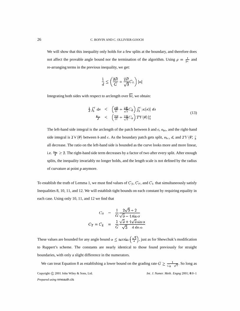
26 C. BOIVIN AND C. OLLIVIER-GOOCH
We will show that this inequality only holds for a few splits at the boundary, and therefore does
not affect the provable angle bound nor the termination of the algorithm. Using � � �� ��� and
re-arranging terms in the previous inequality, we get:
&� �� � �( $ � �
� � ��� . ) � )Integrating both sides with respect to arclength over
� � , we obtain:
���� �� � � � ���� $ �
�
� � ��� � ��� ) � � � � ) � �
������ � ���� $ �
�
� � ��� � ��� � � � ) ��(13)
The left-hand side integral is the arclength of the patch between�
and � , � � � , and the right-hand
side integral is ��� � � � between�
and � . As the boundary patch gets split, � � � � � , and ��� � � � ) ��all decrease. The ratio on the left-hand side is bounded as the curve looks more and more linear,
i.e.������ / �
. The right-hand side term decreases by a factor of two after every split. After enough
splits, the inequality invariably no longer holds, and the length scale is not defined by the radius
of curvature at point anymore.
To establish the truth of Lemma 1, we must find values of � � , ��� , and �� that simultaneously satisfy
Inequalities 8, 10, 11, and 12. We will establish tight bounds on each constant by requiring equality in
each case. Using only 10, 11, and 12 we find that
� � � &( � � � $ �� � , � � ��� �
� � � � � � &( � � $ � � � � ��� �� � , � � ��� �These values are bounded for any angle bound � � � ��� � ��� � � � � , just as for Shewchuk’s modification
to Ruppert’s scheme. The constants are nearly identical to those found previously for straight
boundaries, with only a slight difference in the numerators.
We can treat Equation 8 as establishing a lower bound on the grading rate( / ����
� � . So long as
Copyright c�
2001 John Wiley & Sons, Ltd. Int. J. Numer. Meth. Engng 2001; 0:0–1
Prepared using nmeauth.cls

TRIANGULAR MESH GENERATION WITH CURVED BOUNDARIES 27
(is finite, the mesh will be non-uniform. Relating
(to the angle bound � , we find:
( � � � � � ������� & $ � ���� � , � � �����The minimum theoretical grading rate
(remains finite up to the previously established angle bound.
If the higher bound for(
is used, we have
� � � &� � � ��� ���� � ��� � � � � & $ � � ��� � �� � � � ����� � & $ � � �
In summary, we have established that, for� / & , we can generate meshes with the same angle bounds
as Shewchuk’s modification to Ruppert’s scheme. In the process, we have placed bounds on the grading
rate(
and on the length of the shortest edge in the mesh relative to the local length scale (the constants
� � , � � , and � � give this information).
III. Termination and Size Optimality
We can use the quality lemmas to prove the following theorem about finite mesh size and mesh size
optimality.
Theorem 1. Given a vertex in the output triangular mesh, its nearest neighbor vertex is at a distance
at least ��� � � � � � � $ & � ( � . This implies mesh size optimality.
Proof.
Lemma 1 handles the case where is inserted after . If is inserted last, then we apply the lemma
to :) + , + ) / ���� �
� �
Copyright c�
2001 John Wiley & Sons, Ltd. Int. J. Numer. Meth. Engng 2001; 0:0–1
Prepared using nmeauth.cls

28 C. BOIVIN AND C. OLLIVIER-GOOCH
But ��� � ��/ ����! � $ ���� ���� , so
) + , + ) / ������� , ���� ����� �
and the theorem follows, with only minor algebra.
Because the shortest edge in the mesh must be longer than � ����� ��� �� , each cell has finite size and only
a finite number of them will be required.
We can say more than that. Because the shortest possible edge is within a constant factor of the
length scale locally, the smallest possible triangle is within the square of that same factor of the size
of a triangle whose edges all match the length scale. This implies that the size of the mesh must be
within a constant factor of the size of the smallest possible mesh whose cells meet the quality bound
and whose edges have length within a constant factor of the length scale locally.
Copyright c�
2001 John Wiley & Sons, Ltd. Int. J. Numer. Meth. Engng 2001; 0:0–1
Prepared using nmeauth.cls

FIGURES 29
30o
30o
30o
30o
Figure 1. Comparison between a diametral circle (dashed) and diametral lenses. Diametral lenses allow points tobe inserted closer to boundary edges.
Copyright c�
2001 John Wiley & Sons, Ltd. Int. J. Numer. Meth. Engng 2001; 0:0–1Prepared using nmeauth.cls

30 FIGURES
(a) Small angle causes infinite insertion (b) Concentric circular shells prevent infiniteinsertion
Figure 2. Problem caused by small angles in the domain and how to fix it.
Copyright c�
2001 John Wiley & Sons, Ltd. Int. J. Numer. Meth. Engng 2001; 0:0–1Prepared using nmeauth.cls

FIGURES 31
Midpoint of two verts
Normal at location
Distance from boundary
Initial discretization
Others...
Curvature at location
GenerationAlgorithm
Mesh
Circular Arcs
Others..
Lines
Splines
Information Needed Boundary Patches
Figure 3. Framework used for the implementation of generic boundaries
Copyright c�
2001 John Wiley & Sons, Ltd. Int. J. Numer. Meth. Engng 2001; 0:0–1Prepared using nmeauth.cls

32 FIGURES
Figure 4. Arbitrary original discretization of a spline. No vertex should be inserted in the shaded areas.
Copyright c�
2001 John Wiley & Sons, Ltd. Int. J. Numer. Meth. Engng 2001; 0:0–1Prepared using nmeauth.cls
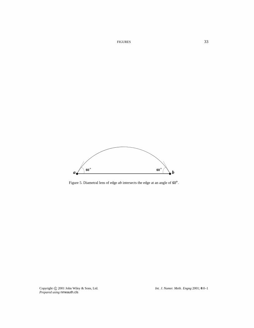
FIGURES 33
60o
60o
a b
Figure 5. Diametral lens of edge ab intersects the edge at an angle of ����� .
Copyright c�
2001 John Wiley & Sons, Ltd. Int. J. Numer. Meth. Engng 2001; 0:0–1Prepared using nmeauth.cls

34 FIGURES
a b
Figure 6. A curve with uniform curvature intersects the edge with angles of ����� .
Copyright c�
2001 John Wiley & Sons, Ltd. Int. J. Numer. Meth. Engng 2001; 0:0–1Prepared using nmeauth.cls

FIGURES 35
Diametral lens outsidethe diametral circle
diametral circle
diametral lens
curve
a
boundary edge
Figure 7. A curve with non-uniform curvature might yield a diametral lens outside the diametral circle.
Copyright c�
2001 John Wiley & Sons, Ltd. Int. J. Numer. Meth. Engng 2001; 0:0–1Prepared using nmeauth.cls

36 FIGURES
Figure 8. Example of an invalid initial discretization
Copyright c�
2001 John Wiley & Sons, Ltd. Int. J. Numer. Meth. Engng 2001; 0:0–1Prepared using nmeauth.cls

FIGURES 37
b c
a
Figure 9. Vertex a should not generate a small feature on edge bc
Copyright c�
2001 John Wiley & Sons, Ltd. Int. J. Numer. Meth. Engng 2001; 0:0–1Prepared using nmeauth.cls

38 FIGURES
Figure 10. Initial discretization of a domain that had overlapping initial boundary edges
Copyright c�
2001 John Wiley & Sons, Ltd. Int. J. Numer. Meth. Engng 2001; 0:0–1Prepared using nmeauth.cls

FIGURES 39
a
b
Figure 11. Example of a feature of the mesh (the small square) that is located in the wrong region due to thediscretization of the curved boundary patch
Copyright c�
2001 John Wiley & Sons, Ltd. Int. J. Numer. Meth. Engng 2001; 0:0–1Prepared using nmeauth.cls

40 FIGURES
Is the edge present?
recoveredGet next edge to be
linear patch?Associated with aIs there a vertex on the
wrong side?
Split edge Swap to recover
Tried swapping forthis edge already?
No
Yes No
No
Yes
NoYes
Yes
Figure 12. Procedure to follow to recover boundary edges
Copyright c�
2001 John Wiley & Sons, Ltd. Int. J. Numer. Meth. Engng 2001; 0:0–1Prepared using nmeauth.cls

FIGURES 41
A
B
C
D
E
Figure 13. The top arc’s discretization crosses over the bottom arc, but does not cross the bottom arc’s discretization
Copyright c�
2001 John Wiley & Sons, Ltd. Int. J. Numer. Meth. Engng 2001; 0:0–1Prepared using nmeauth.cls

42 FIGURES
c
Obtuseangle
b
d
e
a
(a) (b)
Figure 14. Problem associated with curves, small angles, and the use of concentric circular shells.
Copyright c�
2001 John Wiley & Sons, Ltd. Int. J. Numer. Meth. Engng 2001; 0:0–1Prepared using nmeauth.cls

FIGURES 43
Figure 15. Critical points for a Bézier curve
Copyright c�
2001 John Wiley & Sons, Ltd. Int. J. Numer. Meth. Engng 2001; 0:0–1Prepared using nmeauth.cls
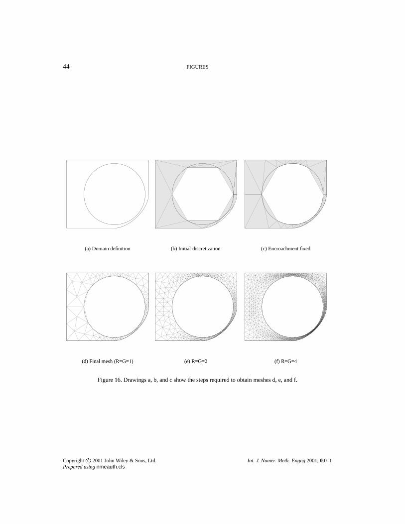
44 FIGURES
(a) Domain definition (b) Initial discretization (c) Encroachment fixed
(d) Final mesh (R=G=1) (e) R=G=2 (f) R=G=4
Figure 16. Drawings a, b, and c show the steps required to obtain meshes d, e, and f.
Copyright c�
2001 John Wiley & Sons, Ltd. Int. J. Numer. Meth. Engng 2001; 0:0–1Prepared using nmeauth.cls

FIGURES 45
Figure 17. Mesh including lines, circles, and arcs as boundary patches. All angles in the mesh are above � � � .
Copyright c�
2001 John Wiley & Sons, Ltd. Int. J. Numer. Meth. Engng 2001; 0:0–1Prepared using nmeauth.cls

46 FIGURES
Figure 18. Mesh with a boundary made up of Bézier curves, lines, and a circle.
Copyright c�
2001 John Wiley & Sons, Ltd. Int. J. Numer. Meth. Engng 2001; 0:0–1Prepared using nmeauth.cls

FIGURES 47
Figure 19. 4-element airfoil mesh.
Copyright c�
2001 John Wiley & Sons, Ltd. Int. J. Numer. Meth. Engng 2001; 0:0–1Prepared using nmeauth.cls

48 FIGURES
(a) After initial discretization
(b) Final mesh, R=G=1
Figure 20. Magnified sections of the 4-element airfoil
Copyright c�
2001 John Wiley & Sons, Ltd. Int. J. Numer. Meth. Engng 2001; 0:0–1Prepared using nmeauth.cls

FIGURES 49
c
a
p
b
r
Figure 21. Lemma 1, Statement 2: � added as circumcenter of large triangle � .
Copyright c�
2001 John Wiley & Sons, Ltd. Int. J. Numer. Meth. Engng 2001; 0:0–1Prepared using nmeauth.cls

50 FIGURES
cp
b
θ
r
r’
a
Figure 22. Lemma 1, Statement 3: � added as circumcenter of badly shaped triangle � .
Copyright c�
2001 John Wiley & Sons, Ltd. Int. J. Numer. Meth. Engng 2001; 0:0–1Prepared using nmeauth.cls

FIGURES 51
a
r’
cb
p
DiametralDiametral
lens circle
2d
Figure 23. Lemma 1, Statement 4: � added to split an encroached boundary edge.
Copyright c�
2001 John Wiley & Sons, Ltd. Int. J. Numer. Meth. Engng 2001; 0:0–1Prepared using nmeauth.cls

52 TABLES
Parameters Angles (in degrees) Edge length ratiosFigure number R G Min Max Min Avg Max
16 1 1 30.01 104.08 0.2500 0.8819 1.85982 2 35.11 104.42 0.4362 0.8937 2.0014 4 32.56 114.88 0.4547 0.9173 1.8015
17 4 4 33.85 108.15 0.3811 0.9223 1.755218 4 4 33.31 110.06 0.1257 0.9003 1.966419 1 1 30.89 111.21 0.0669 0.3686 3.4170
Table I. Quality measures
Copyright c�
2001 John Wiley & Sons, Ltd. Int. J. Numer. Meth. Engng 2001; 0:0–1Prepared using nmeauth.cls