m0

Guaranteed-Quality Triangular Meshes

DTICiI ELECTED

L. Paul Chewo JUL 1 41989

TR 89-983 SApril 1989D

Department of Computer ScienceCornell UniversityIthaca, NY 14853-7501

DISTRMIMON STATEMENT A

Approved for public releow*_. Dii) utioz Unlimited

'This research has been sul ported by NSF grant E it-86-17355, ONR grant N0014-86-K-0281, and DA.RPA un lerONR contract N00014-88-K-0591..

TIM views and cvonc-rIsionn. containe, in this document .etm thoneOf th.& authors and should not be I erpratcd an neces.sarilyrepresenting the official policies, either expresned or impLied,of the Defense Ad, :ed Research P: jects Pgency or the U.S-Gower ment°

iI

Guaranteed-Quality Triangular Meshes

DTICELECTE

L. Paul Chew* JUL 1419891TR 89-983 SApril 1989

Department of Computer ScienceCornell Universityithaca, NY 14853-7501

ZLiSTFLMhUION STAEMENr AL Approved for public teleozelL_ Dism~butoa Unlimited

*This research has been supported by NSF grant DCM-86-17355, ONR grant N0014-86-K-0281, and DARPA underONR contract N00014-88-K-0591..

The views and conclusionL contained In this document are thoseof the authors and should not be interpreted as necessarilyrepresenting the official policies, either expressea or impUed,of the Defense Advanced Research Projects hgency or tlhe U.S.Governent.

Accesion FDr

NTIS CRA&-DTIC TAB UUnanno, ,JJustifirJu.- •Guaranteed-Quality Triangular Meshes

AA\llbifitY Codes L. Paul ChewDepartment of Computer Science

AvaS iado Cornell UniversityDIsi Special _Ithaca, NY 14853

Abstract

There are a number of applications for which it is desirable to divide a given

region in the plane into nicely shaped triangles. One important such

application is the finite element method, a method widely used to obtain

approximate solutions to a wide variety of engineering problems. For this

kind of application, not just any triangulation will do; error bounds are best if

all the triangles are as close as possible to equilateral triangles. Presently,

either these triangulations are produced by hand or they are produced

automatically using one of a number of heuristic techniques. For these

heuristic techniques, certain cases can require human intervention to

eliminate flat triangles. In this paper, we present an efficient new technique

(based on Delaunay triangulations) for automatically producing desirable

triangulations. Unlike most previous techniques, this one comes with a

guarantee: the angles in the resulting triangles are all between 30'd and 120O.9--.

and the edge lengths are all between h and 2h where h is a parameter chosen

by the user. Additional useful properties include (I) the worst-case time to

produce a triangulation is linear in the final number of triangles, and (2) the

user can control the element density, producing smaller triangles in areas

where more accuracy is desired. ,j ,

Work on this paper has been supported by NSF grant DMC-86-17355, ONR grant N0014-86-K-0281, and DARPA under ONR contract N0014-88-K-0591.

Tue. Apr 4, 1989

1. Introduction.

We study the following problem: given a polygonal region in the plane,

divide the region into triangles in such a way that the triangles are as close as

possible to equilateral triangles. We refer to the process of dividing a region

into triangles as triangulation and the resulting set of triangles is called a

triangular mesh for the region. A program for creating a mesh is called an

automatic mesh generator. The reader should note that unlike many

triangulation problems (e.g., triangulating a set of points in the plane) in

which only edges are introduced, an automatic mesh generator can introduce

both new vertices and new edges.

This problem is motivated by the requirements of the finite element

method, a widely used technique for obtaining approximate numerical

solutions to a wide variety of engineering problems. Given a problem, the

first step of the finite element method is to divide the problem region into

finitely many simply-shaped regions called elements, creating a finite

element mesh. In two dimensions, this usually means dividing a given region

into either triangles or quadrilaterals. Triangular elements are sometimes

preferred because of the ease with which they can be made to fit complex

boundaries. Not just any triangulation will do; error bounds are best if the

triangles are as close as possible to equilateral triangles. (For more

information on the finite element method, see, for instance, [HT82, OR76, SF73,

or Zi771.)

Triangulating a planar region by hand (i.e., using a mouse or other input

device and a graphics terminal) can be a tedious process; thus, a number of

automatic mesh generators have been developed (for instance, [BW&87, Ca74,

CFF85, Fr87, Jo86, JS86, Lo85, YS83], and many others; [Sh88, Si79, and Th80J are

survey papers on this subject). Several of these mesh generators use an

iterative smoothing process to improve the resulting meshes. Even with

smoothing, these algorithms do not provide a guarantee about the quality of

Tue, Apr 4, 1989 2

the result, and human intervention may sometimes be required to improve the

triangulation.

In this paper, we present a new algorithm for triangulating planar

regions. Unlike most previous methods, this new algorithm comes with a

guarantee: for a triangulation produced by the algorithm, all angles are

between 300 and 1200 and all edge lengths are between h and 2h where h is a

parameter chosen by the user. In addition, the algorithm can be implemented

to run in worst-case time O(n) where n is the number of triangles in a

triangulation produced by an imaginary perfect triangulation algorithm.

Further, the user can control the element density, producing smaller triangles

in areas where more accuracy is desired.

The guarantee associated with this algorithm is particularly important.

Without such a guarantee, an automatic mesh generator may sometimes

require human inspection of the mesh. One problem with this requirement is

that it is inappropriate for the naive user of the finite element method. More

significantly, this requirement is inappropriate for even the expert user

when solving problems where many meshes need to be generated, such as

problems involving adaptive remeshing, or problems where the geometry

changes over time. A guaranteed-quality mesh generator can make human

inspection of the mesh unnecessary.

Baker, Grosse, and Rafferty [BGR88] have also presented a 2Dtriangulation algorithm that includes a guarantee. They use a completely

different technique for which the resulting angles are guaranteed to be

between 13' and 900. They place a grid over the region to be triangulated and

observe that each interior cell can be triangulated with a single diagonal.

They then develop methods for triangulating the boundary cells. This

technique leads to small triangles near the boundary of the given region.

In the next section we explain some of the background necessary for

understanding the guaranteed-quality triangulation algorithm. In Section 3

we explain the basic algorithm. The linear time version of the algorithm is

Tue, Apr 4. 1989 3

explained in Section 4, and section 5 contains a comparison of the algorithm

with an imaginary perfect triangulation algorithm. Section 6 explains how

the sizes of the elements may be varied across a region. Finally, Section 7

presents some conclusions and further research.

2. Background - Delaunay Triangulations.

Like some earlier techniques ([CFF85, Fr87, and Jo86J, for instance) the

guaranteed-quality triangulation technique is based on properties of

Delaunay triangulations. In this section we present some of the properties of

the Delaunay triangulations and we explain a special type of Delaunay

triangulation, called a constrained Delaunay triangulation, which has

characteristics particularly useful for mesh generators.

A Voronoi diagram and the corresponding Delaunay triangulation.

The Delaunay triangulation of a set S of points in the plane is most easily

introduced by reference to the Voronoi diagram of S (also called the

Dirichlet tessalation of S). The Voronoi diagram of S divides the plane into

regions, one region for each point in S, such that for each region R and

corresponding point p, every point within R is closer to p than to any other

Tue, Apr 4, 1989 4

point of S. The boundaries of these regions form a planar graph. The

Delaunay triangulation of S is the straight-line dual of the Voronoi diagram of

S; that is, we connect a pair of points in S iff they share a Voronoi boundary.

The Voronoi diagram and its dual, the Delaunay triangulation, have been

found to be among the most useful data structures in computational geometry.

See lEd87 or PS85] for a number of Voronoi diagram and Delaunay

triangulation applications.

Each triangle of the Delaunay triangulation of S has the empty circle

property: a circle circumscribed about a Delaunay triangle contains no

points of S in its interior. Indeed, this property can be used as the definition

of Delaunay triangulation.

A Delaunay triangulation and the corresponding empty circles.

Definition. Let S be a set of points in the plane. A triangulation T is a

Delc.unay triangulation of S if for each triangular face A of T there exists a

circle C with the following properties:

1. C circumscribes A, and

2. no vertex of- S is in the interior of C.

A circle circumscribed about about a Delaunay triangle is called a Delaunay

Tue, Apr 4, 1989 5

circle. If S contains 4 points that are cocircular then the Delaunay

triangulation is not necessarily unique. For our purposes, if there is not a

unique Delaunay triangulation then any of them will do.

The Delaunay triangulation has some properties indicating that it might

lead to good finite element meshes. In particular, the Delaunay triangulation

maximizes the minimum angle for a set of points. In other words, among all

triangulations of a given set of points, the Delaunay triangulation has the

largest minimum angle (see, for instance, [Ed87I).

Unfortunately, the Delaunay triangulation is not quite what is needed to

make triangulations for the finite element method. The problem is, for a finite

element mesh, certain edges must be used as part of the final triangulation

(e.g., those that describe the boundaries or, perhaps, those that describe a

crack in the object to be analyzed). Such edges do not always correspond to

legal Delaunay edges. Schroeder and Shephard [SS88] discuss some of the

difficulties of using a Delaunay triangulation to create a mesh for an object.

Many of these difficulties can be resolved by using a constrained

Delaunay triangulation (CDT). Intuitively, a CDT is as close as possible t, a

Delaunay triangulation given that certain prespecified edges must be included

in the triangulation. Compare the definition of the CDT with the definition of

the (unconstrained) Delaunay triangulation given above.

Definition. Let G be a straight-line planar graph. A triangulation T of the

vertices of G is a constrained Delaunay triangulation (CDT) of G if each edge of

G is an edge of T and for each triangular face A of T there exists a circle C with

the following properties:

1. C circumscribes A, and

2. if any vertex v of G is in the interior of C then it cannot be "seen"

from at least one of the vertices of A (i.e., if you draw the line

segments from v to each vertex of A then at least one of the line

segments crosses an edge of G).

Tue, Apr 4, 1989 6

0

A graph 0 and the corresponding constrained Delaunay triangulation.

The same term, Delaunay circle, is used for a circle circumscribed about

either a standard Delaunay triangle or a CDT triangle. The CDT, also called a

generalized Delaunay triangulation [Le78, LL86], was first introduced by Lee.

O(n 2 ) time algorithms for constructing the CDT of a straight-line planar graph

G (with n vertices) are given in [DFP85 and LL86]. An asymptotically-optimal,

O(n log n) worst-case time algorithm appears in [Ch89a]. Surprisingly, the

triangulation technique introduced in Section 4 can be implemented to

triangulate a region in worst-case linear time (linear in the number of

triangles produced) even though the resulting triangulation is a CDT.

Applications of CDTs appear in [Ch89a, Ch89b, DFP85, Le78, and LL86].

3. How to Triangulate.

In this section we present one version of our automatic mesh generator.

We show how properties of the CDT can be used to prove that the triangles in

the resulting mesh are of guaranteed quality. The algorithm presented in this

section is relatively slow, requiring O(n 2 ) time in the worst case (n is the

number of triangles in the final triangulation). Section 4 contains a

modification of this algorithm that creates a guaranteed-quality triangulation

Tue, Apr 4, 1989 7

in worst-case linear time.

There are some undemanding preconditions that the initial problem must

satisfy. The input to the algorithm is a set of data points and data edges.

Basically, these points and edges are those necessary to describe the boundary

of the region, but, in fact, we allow the user to specify additional points and

edges. All points and edges specified at this stage will appear in the final

triangular mesh. The data points and data edges must satisfy the following two

conditions (recall that h is a parameter chosen by the user; intuitively, it

represents the desired side-length of triangles in the triangulation):

1. No two data points are closer than h.

2. All data edges have lengths between h and (43)h.

In practice, it is trivial to subdivide long edges to comply with condition two,

except for edges with lengths between (3)h and 2h. Later in this section, we

show how these edges can, in effect, be hidden, although when this is done,

care must be taken to ensure that condition 1 is not compromised.

Preconditions:The input is a set of data points and data edges. This set describes theregion to be triangulated, but may include additional data points and dataedges. No two data points are closer than h. All data edges have lengthsbetween h and (43)h.

Algorithm:beginCompute the CDT of the data points and data edges;Let T be the portion of the CDT that is within the region to be triangulated;while there is a Delaunay circle within T that has radius > h do

Add the center of the Delaunay circle as a new data point;Recompute T;end while;

Report T as the desired triangulation;end.

Tue, Apr 4, 1989 8

Add the center point of a large-radius Delaunay circle and recompute the CDT.

Theorem 1. T, the final triangulation produced by the preceding algorithm,

satisfies the following two properties.

1. No two vertices of T are closer than h.

2. Every triangle of T fits within a circle of radius :< h.

Proof. First, note that property 1 holds when the algorithm begins and

continues to hold throughout the execution of the algorithm. To see this, note

that all points added are at the centers of Delaunay circles with radius greater

than h.

Second, no point is closer than distance h/2 to a data edge. To see this,

consider a point p and let e be the closest edge to p. Since e has length < (43)h,

if point p is closer than h/2 to such an edge then it is also closer than h to an

endpoint of the edge, a contradiction.

Finally, it is obvious that property 2 holds if the algorithm halts. To see

that it halts, note that for each new point added during the execution of the

algorithm, the circle of radius h/2 about the point is empty, containing no

other points and no portions of data edges. Further, from property 1, it is clear

Tue, Apr 4, 1989 9

that these circles do not overlap. Only finitely many such circles can fit

within a bounded region; thus, since a new circle is added each time through

the loop, the algorithm must halt. 0

Corollary. T, the final triangulation produced by the preceding algorithm,

satisfies the following additional properties.

3. All edges of T have lengths between h and 2h.

4. All angles of T are between 300 and 1200.

Proof. Property 3 obviously follows from properties 1 and 2. To see that

property 4 also follows, consider any triangle of the triangulation and let a be

the smallest angle of that triangle. From property 2, the circle circumscribed

about the triangle has radius < h, and from property 1, the edge opposite angle

x has length 2t h. It immediately follows that the central angle corresponding

to a is > 60 and a itself is - 300. Once we know the smallest angle is > 30, it is

clear that the greatest angle is ! 1200. 0

The second precondition (all data edges have length between h and (413)h)

can be relaxed. Of course, for an edge longer than 2h, new data points can be

introduced to divide the edge into pieces with lengths in the required range.

However, if an edge has length between ('13)h and 2h, a problem occurs: such

an edge cannot be divided into appropriately sized pieces. This difficulty can

be avoided by, in effect, hiding such edges. To do this, place a new data point

in the interior of the region to make a 450 isosceles triangle (with the problem

edge as its hypotenuse); connect the endpoints of the problem edge to this new

data point. These new edges have lengths in the required range. Now, when

the algorithm is executed, no points can be placed within the triangle (such a

new point would be too close to one of the vertices of the triangle) and the

triangle itself satisfies the prooerties of the theorem (it fits within a circle of

Tue, Apr 4, 1989 10

radius h and no two of its points are closer than h). Of course, care must be

taken to ensure that any new data point introduced to hide an edge is no closer

than h to any other data point.

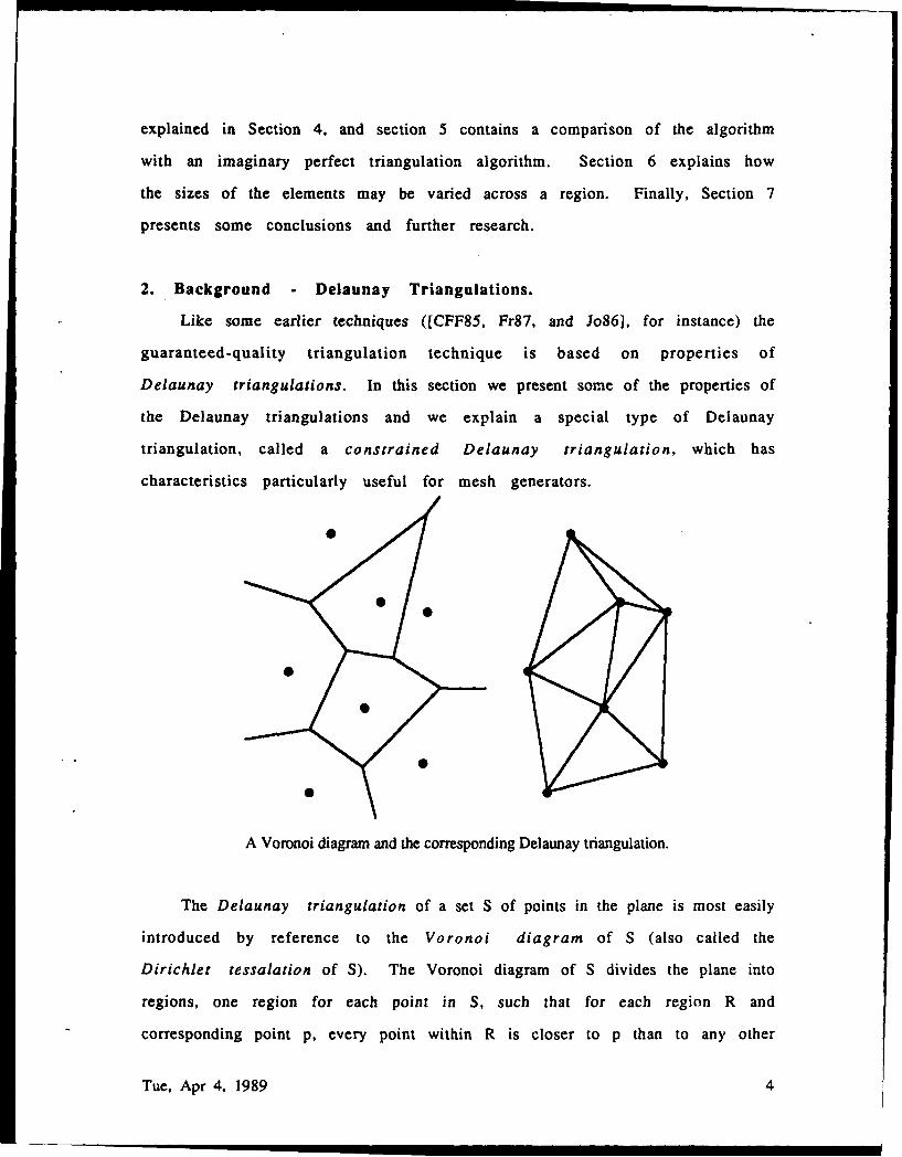
The algorithm as outlined in this section can be implemented to run in

worst-case time O(n 2 ), where n is the number of triangles in the final

triangulation. The initial CDT can be built in time O(n log n) [Ch89a] or, using

a simpler algorithm, in time O(n 2 ). Each point that is inserted can require up

to O(n) processing to update the CDT, giving a total time of O(n 2 ) for the entire

algorithm.

4. How to Triangulate in Optimal Time.

This section contains an outline of the optimal time algorithm. For the

optimal time algorithm, we look at the triangulation problem a little

differently; instead of starting with data points and data edges and building a

triangulation, we start with an independent triangulation and modify it as we

add the data points and data edges. We assume the data points and data edges

satisfy the preconditions stated above. In addition, we assume that the data

points and edges form a connected graph. (The algorithm can be modified to

handle multiple components.) Data points will be added to the triangulation in

depth-first-search order.

We start with a regular grid of equilateral triangles with edge length

(43)h and large enough to cover the region to be triangulated. We assume that

this regular grid is precomputed; the time needed to construct this grid is not

counted as part of the running time of the algorithm. Note that the grid itself

is the Delaunay triangulation (also the CDT) of its own vertices. We call these

vertices grid points to distinguish them from the data points describing the

region to be triangulated. Initially, T consists entirely of this simple CDT, a

triangulation using only grid points and no data points. The data points are

added one at a time to T in depth-first-search order; when a data point is added

we also add any data edges between it and data points already in T. Depth-first-

Tue, Apr 4, 1989 11

search order is used so that we never have to search T to find where to put a

data point; a data point is always placed near a previous data point.

T is modified after each addition to ensure that T is always a CDT and to

ensure that T satisfies the properties of Theorem 1. To do this, we execute the

following steps:

(1) Eliminate any points closer than h to the new data point;

(2) Make T into a CDT again;

(3) while there exists a large (radius>h) Delaunay circle do

Add the circle's center point and make T into a CDT again.

The important observation is that all these changes to T are local changes

(within radius 4h of the newly added data point). This observation can be used

to show that the algorithm runs quickly. Since the only changes in the

diagram are within radius 4h of the new point, and since the points of T

cannot be too close to each other, the number of points affected by a newly

added data point can be bounded by a small constant. In other words, it takes

just constant time to update T for each new data point; thus, the total time is

0(n) where n is the number of data points.

There are many possible variations on this algorithm depending on the

triangular mesh desired. For instance, the edge length in the initial grid can

be different. It also works with a regular grid of squares (with diagonals added

to make triangles) or rectangles. It is even possible to start with an irregular

grid provided the grid is a Delaunay triangulation in which each Delaunay

circle has radius less than h.

5. Comparison with an Optimal Triangulation.

In this section we show that the guaranteed-quality triangulation

algorithm produces an optimal number of triangles. In other words, any mesh

generator that produces a mesh in which the edge length is about h, will

Tue, Apr 4, 1989 12

produce about the same number of triangles. Thus, the linear time version

described in the previous section is optimal in the sense that any mesh

generating algorithm will have to take at least linear time just to report the

mesh.

An imaginary perfect triangulation algorithm would allow the user to

specify the parameter h and would then completely divide a given region into

equilateral triangles where all triangles have edges of length h. Of course, not

every region can be subdivided in this way, but such a triangulation

represents an ideal goal. Each equilateral triangle in such a triangulation has

area ('43)h/4; thus, if A is the area of the region to be triangulated then the

number of triangles is 4A/(h'43).

Our technique matches this ideal goal. The area of the smallest possible

triangle that can be produced by this technique is (43)h/4; thus, the maximum

number of triangles that can be produced for a region of area A is (4A)/(hq 3).

In other words, the guaranteed-quality triangulation algorithm presented

here creates about the same number of triangles as an imaginary ideal

algorithm.

6. Varying the Density.

It is sometimes desirable to divide a region into triangles of different

sizes. For example, for the finite element method, small elements generally

give greater accuracy than large elements, but it takes longer to process small

elements. Because of this, it can be desirable to have small elements where

something interesting is occurring (e.g., near the boundary of the region) to

ensure accuracy, with large elements elsewhere (e.g., in the interior of the

region) to save processing time. In this section we describe one way in which

the element density can be varied without compromising the quality of the

resulting mesh. To do this, we create artificial boundaries.

To see how this can be done, recall the precondition needed by the

Tue. Apr 4, 1989 13

guaranteed-quality triangulation algorithm: all boundary edges must have

lengths between h and (43)h. This was the necessary precondition for using

circles of radius h. If we use circles with radius ('43)h then the precondition

for the edge lengths must be altered in proportion; in this case, all boundary

edges would be required to have lengths between ('43)h and 3h. Note that if a

boundary consists entirely of edges of length (43)h, then on one side of the

boundary we can use circles of radius h and on the other side we can use

circles of radius (43)h.

This idea can be used to vary the element density by inserting artificial

boundaries between regions of different density. Wherever we want a change

in the size of triangles, we insert an artificial boundary, allowing the element

size to change across the boundary by a factor of 43. If a larger factor is

desired then more artificial boundaries can be used. In practice, it may not be

desirable to allow 43 size jumps because of the difficulty of getting all the edges

of an artificial boundary to have exactly the same length, but it should easy

enough to allow jumps of size, say, 3/2.

7. Conclusions and Further Research.

Provided the input satisfies some undemanding preconditions, the

triangulation technique introduced in this paper has the following properties:

(1) the resulting triangulation contains only nicely shaped triangles;

(2) the user can vary the triangle sizes over the region;

(3) the number of triangles produced is near optimal; and

(4) the technique can be implemented to run in optimal, linear time.

In addition, the technique may lead to a number of interesting applications

and extensions.

The guaranteed-quality technique should be applicable to the

triangulation of shells (curved surfaces). Basically, instead of looking at

Delaunay circles, we look at the corresponding spheres where a sphere is

constrained to have its center on the surface.

Tue, Apr 4, 1989 14

In addition to the finite element method, other application areas for

guaranteed-quality triangulations include virtually any problem where it is

desirable to choose a set of points that evenly fills a given region in the plane

or that evenly covers a given surface. For instance, in (DJ8"/J a set of sample

points describing a surface is used to detect errors in numerically controlled

machining. The triangulation technique presented here, altered to work for

surfaces, gives a good way to select the sample points. There are other possible

uses in graphics and geology.

Of particular interest, is the possibility of extending the algorithm

presented here to develop a guaranteed-quality mesh generator for problems

in three dimensions. For the finite element method in three dimensions, the

goal is to divide an object into nicely shaped tetrahedra (or hexahedra or

triangular prisms). We refer to the process of dividing an object into

tetrahedra as 3D triangulation.

The basis of the 2-dimensional technique, the Delaunay triangulation,

extends nicely to 3 dimensions, producing tetrahedra with nicely shaped faces.

Unfortunately, a guarantee about the shapes of the tetrahedral faces does not

imply a guarantee about the quality of the tetrahedra; in the terminology of

[CFF85I, slivers can occur. Slivers are tetrahedra with well-proportioned

faces, but with arbitrarily small volume. An example is the degenerate

tetrahedron defined by 4 points equally spaced around the equator of a sphere.

Several heuristic techniques for 3D triangulation have been developed

[CFF85, Fi86, PP&88, and YS841; [Sh88] surveys several 3D triangulation

techniques. These techniques are heuristic in the sense that there is no

guarantee about the quality of the resulting 3D mesh. A 3D triangulation

technique with guaranteed performance, a technique for which all tetrahedra

are guaranteed to be close to regular tetrahedra, would be of significant

interest in Computer Aided Design.

Tue. Apr 4. 1989 15

References

[BGR88] B. S. Baker, E. Grosse, C. S. Rafferty, Nonobtuse Triangulation ofPolygons, Discrete and Computational Geometry, 3 (1988), 147-168.

[BW&87] P. L. Baehmann, S. L. Wittchen, M. S. Shephard, K. R. Grice, and M. A.Yerry, Robust, geometrically based, automatic two-dimensional meshgeneration, International Journal for Numerical Methods inEngineering, 24 (1987), 1043-1078.

[Ca74) - J. C. Cavendish, Automatic triangulation of arbitrary planar domainsfor the finite element method, International Journal for NumericalMethods in Engineering, 8 (1974), 679-696.

[CFF85] J. C. Cavendish, D. A. Field, and W. H. Frey, An approach to automaticthree-dimensional finite element mesh generation, International

Journal for Numerical Methods in Engineering, 21 (1985), 329-347.

[Ch89a] L. P. Chew, Constrained Delaunay triangulations, Algorithmica, 4(1989), 97-108.

[Ch89b] L. P. Chew, There are planar graphs almost as good as the completegraph, JCSS, to appear.

[DFP85] L. De Floriani, B. Falcidieno. and C. Pienovi, Delaunay-basedrepresentation of surfaces defined over arbitrarily shaped domains,

Computer Vision, Graphics, and Image Processing, 32 (1985), 127-140.

[DJ87] R. L. Drysdale and R. B. Jerard, Discrete simulation of NC machining,Proceedings of the Third Annual Symposium on Computational

Geometry, (1987), 126-135.

lEd87] H. Edelsbrunner, Algorithms in Combinatorial Geometry, Springer-Verlag (1987).

[Fi86] D. A. Field, Implementing Watson's algorithm in three dimensions,Proceedings of the Second Annual Symposium on ComputationalGeometry, (1986), 246-259.

Tue, Apr 4, 1989 16

[Fr87] W. H. Frey, Selective refinement: a new strategy for automatic node

placement in graded triangular meshes, International Journal for

Numerical Methods in Engineering, 24 (1987), 2183-2200.

[HT821 K. H. Huebner and E. A. Thornton, The Finite Element Method for

Engineers, John Wiley & Sons (1982).

[Jo86] B. Joe, Delaunay triangular meshes in convex polygons, SIAM J. Sci.

Stat. Comput., 7:2 (1986), 514-539.

[JS86] B. Joe and R. B. Simpson, Triangular meshes for regions of

complicated shape, International Journal for Numerical Methods in

Engineering, 23 (1986), 751-778.

[Le781 D. T. Lee, Proximity and reachability in the plane, Technical Report

R-831, Coordinated Science Laboratory, University of Illinois (1978).

[LL86] D. T. Lee and A. K. Lin, Generalized Delaunay triangulation for planar

graphs, Discrete and Computational Geometry, 1 (1986), 201-217.

[Lo85] S. H. Lo, A new mesh generation scheme for arbitrary planar

domains, International Journal for Numerical Methods in

Engineering, 21, 1403-1426 (1985).

[OR76] J. T. Oden and J. N. Reddy, An Introduction to the Mathematical

Theory of Finite Elements, John Wiley & Sons (1976).

[PP&88] J. Peraire, J. Peiro, L. Formaggio, K. Morgan, and 0. C. Zienkiewicz,

Finite element Euler computations in three dimensions,

International Journal for Numerical Methods in Engineering, 2 6

(1988), 2135-2159.

[PS851 F. P. Preparata and M. I. Shamos, Computational Geometry,

Springer-Verlag (1985).

[SF731 G. Strang and G. J. Fix, An Analysis of the Finite Element Method,

Prentice-Hall (1973).

Tue, Apr 4, 1989 17

[Sh88] M. S. Shephard, Approaches to the automatic generation and control

of finite element meshes, Applied Mechanics Reviews, 41:4 (April

1988), 169-185.

[Si79] R. B. Simpson, A survey of two dimensional finite element mesh

generation, Proc. of the Ninth Manitoba Conference on NumericalMath. and Computing, (1979), 49-124.

[SS88] W. J. Schroeder and M. S. Shephard, Geometry-based fully automaticmesh generation and the Delaunay triangulation, International

Journal for Numerical Methods in Engineering, 26 (1988), 2503-

2515.

[Th80] W. C. Thacker, A brief review of techniques for generating irregular

computational grids, International Journal for Numerical Methods

in Engineering, 15 (1980), 1335-1341.

[YS83] M. A. Yerry and M. S. Shephard, A modified quadtree approach tofinite element mesh generation, IEEE Computer Graphics & Appl.,

3:1 (1983), 39-46.

[YS84] M. A. Yerry and M. S. Shephard, Automatic three-dimensional mesh

generation by the modified-octree technique, International Journalfor Numerical Methods in Engineering, 20 (1984), 1965-1990.

[Zi77] 0. C. Zienkiewicz, The Finite Element Method, McGraw-Hill (1977).

A

Tue, Apr 4, 1989 18