Embed Size (px)
Citation preview

TECHNICAL UNIVERSITY DRESDEN
DEPARTMENT OF COMPUTER SCIENCE
INSTITUTE OF SOFTWARE AND MULTIMEDIA TECHNOLOGY
CHAIR OF COMPUTER GRAPHICS AND VISUALIZATION
PROF. DR. STEFAN GUMHOLD
Großer Beleg
Simulating the design of a CIP system by means ofComputer Graphics techniques
Katrin Braunschweig(Mat.-No.: 3017128)
Tutor: Sören König
Dresden, October 29, 2008


Aufgabenstellung
Zielstellung:
Bei der automatisierten Reinigung von Verarbeitungsmaschinen kommen sog. Cleaning in Place-Systeme
zum Einsatz. Die Durchführung der Säuberung erfolgt u.a. mit speziell platzierten Sprühreinigungs-
düsen. Die Wirksamkeit solcher Systeme wird momentan durch Versuche an der Maschine getestet, was
diverse Nachteile (hoher Aufwand, hohe Kosten, schlechtes Hygenic Design, keine optimale Auslegung
der Versorgungsanlage) hat.
Ziel dieser Arbeit ist die Untersuchung der Übertragbarkeit von Ansätzen aus der Computergraphik zur
Simulation und Optimierung des Sprühreinigungsvorgangs.
Teilaufgaben:
• Computergestützte Modellbildung des Sprühreinigungsvorgangs (Düsenplatzierung, Sprühkegel,
Sprühschatten, ...)
• Erarbeitung von Lösungsstrategien verwandter Problematiken wie z.B. der Beleuchtungssimula-
tion oder des Scan-View-Plannings.
• Export von CAD - Baugruppen (Testdaten) in ein geeignetes Format für die Simulation
• Realisierung eines Softwareprototyps für die Berechnung der Simulation
• Visualisierung des Wirkbereiches der Sprühdüsen (Simulationsergebnis)
Kür:
• Erarbeitung gewünschter/möglicher Optimierungsstrategien (in Kooperation mit Maschinenbau)
und mögliche Lösungsstrategien zur Platzierung und Ausrichtung der Sprühdüsen


1
Contents
1 Introduction 3
1.1 Motivation . . . . . . . . . . . . . . . . . . . . . . . . . . . . . . . . . . . . . . . . . . 3
1.1.1 CIP systems . . . . . . . . . . . . . . . . . . . . . . . . . . . . . . . . . . . . . 3
1.1.2 3D computer simulation . . . . . . . . . . . . . . . . . . . . . . . . . . . . . . 4
1.1.3 Purpose of study . . . . . . . . . . . . . . . . . . . . . . . . . . . . . . . . . . 5
1.2 Task specification . . . . . . . . . . . . . . . . . . . . . . . . . . . . . . . . . . . . . . 6
1.3 Outline . . . . . . . . . . . . . . . . . . . . . . . . . . . . . . . . . . . . . . . . . . . 6
2 Background and related work 7
2.1 Cleaning in place systems . . . . . . . . . . . . . . . . . . . . . . . . . . . . . . . . . . 7
2.2 Computer Graphics methods . . . . . . . . . . . . . . . . . . . . . . . . . . . . . . . . 7
2.2.1 3D representation of CIP system components . . . . . . . . . . . . . . . . . . . 8
2.2.2 Fluid - surface interaction . . . . . . . . . . . . . . . . . . . . . . . . . . . . . 11
2.2.3 Visualization of interaction features . . . . . . . . . . . . . . . . . . . . . . . . 13
3 Requirements and implementation 17
3.1 3D representation of the CIP system components . . . . . . . . . . . . . . . . . . . . . 17
3.1.1 Fluid representation . . . . . . . . . . . . . . . . . . . . . . . . . . . . . . . . 17
3.1.2 Spray nozzle representation . . . . . . . . . . . . . . . . . . . . . . . . . . . . 19
3.1.3 Object representation . . . . . . . . . . . . . . . . . . . . . . . . . . . . . . . . 25
3.1.4 Transformation . . . . . . . . . . . . . . . . . . . . . . . . . . . . . . . . . . . 29
3.2 Interaction between fluid and objects . . . . . . . . . . . . . . . . . . . . . . . . . . . . 31
3.2.1 Ray-object intersection . . . . . . . . . . . . . . . . . . . . . . . . . . . . . . . 32
3.2.1.1 Line-triangle intersection . . . . . . . . . . . . . . . . . . . . . . . . 32
3.2.1.2 Parabola-triangle intersection . . . . . . . . . . . . . . . . . . . . . . 34
3.2.2 Acceleration methods . . . . . . . . . . . . . . . . . . . . . . . . . . . . . . . . 35
3.2.2.1 Kd-tree construction . . . . . . . . . . . . . . . . . . . . . . . . . . . 36
3.2.2.2 Kd-tree traversal . . . . . . . . . . . . . . . . . . . . . . . . . . . . . 40

2
3.2.2.3 Ray-box intersection . . . . . . . . . . . . . . . . . . . . . . . . . . . 43
3.2.3 Recursive ray tracing . . . . . . . . . . . . . . . . . . . . . . . . . . . . . . . . 46
3.3 Collection of intersection data . . . . . . . . . . . . . . . . . . . . . . . . . . . . . . . 49
3.3.1 Intersection information . . . . . . . . . . . . . . . . . . . . . . . . . . . . . . 49
3.3.2 Texture atlas . . . . . . . . . . . . . . . . . . . . . . . . . . . . . . . . . . . . 51
3.3.2.1 Unfolding . . . . . . . . . . . . . . . . . . . . . . . . . . . . . . . . 52
3.3.2.2 Packing . . . . . . . . . . . . . . . . . . . . . . . . . . . . . . . . . 56
4 Results 59
4.1 Functionality . . . . . . . . . . . . . . . . . . . . . . . . . . . . . . . . . . . . . . . . 59
4.2 Issues . . . . . . . . . . . . . . . . . . . . . . . . . . . . . . . . . . . . . . . . . . . . 64
4.3 Performance . . . . . . . . . . . . . . . . . . . . . . . . . . . . . . . . . . . . . . . . . 71
5 Future work 75
6 Conclusion 77
Bibliography 79
List of Figures 83

3
1 Introduction
These days, a big part of the goods we consume or pharmaceutical products we use are produced or
processed industrially in automated processes in modern facilities. The goal is to reach a high efficiency,
producing goods in large quantities in short time while at the same time keeping the expenses to a mini-
mum. But especially the companies producing consumer goods or pharmaceuticals are bound to special
guidelines regarding the sanitary conditions of the facilities. The cleaning necessary to meet the sanitary
standards causes additional costs and an increased water consumption. Many companies use cleaning
in place (CIP) or cleaning out of place (COP) systems, to clean their facilities. But considering the cur-
rent environmental issues, it is important to use the water reasonably. Therefore the water consumption
should be taken into account during the design of the cleaning system. Since computers are used in
many applications nowadays, ranging from the design of a product to the construction and assembly or
the automation of a process, using computers could also be helpful for the design of a cleaning system
that keeps the water consumption to a minimum.
This project takes a look at the feasibility of simulating a cleaning system on a computer with the help
of established algorithms from the field of 3D Computer Graphics.
1.1 Motivation
This project focuses on cleaning in place (CIP) systems, not on cleaning out of place systems or other
cleaning systems.
1.1.1 CIP systems
Cleaning in Place (CIP) is the process of cleaning production or storage facilities without dismantling.
A CIP system generally consists of storage and mixing facilities for the cleaning liquid, pipework to
circulate the liquid, spray nozzles and an automation system controlling the setting in addition to the
tank or vessel that is to be cleaned. The cleaning liquid is directed from the storage tank through the
pipes towards the facility that needs to be cleaned. Via various types of spray nozzles, which can be fixed

4 1. INTRODUCTION
or rotating, the cleaning liquid is sprayed onto the surface of the facility in order to remove soil. Some
CIP systems only use the liquid once, directly discharging it into the drain after use. Other systems reuse
the liquid depending on the level of contamination. During one cleaning cycle a facility can be sprayed
with several different liquids successively, to remove different types of soil. In between the spraying with
different cleaning liquids, the facility needs to be rinsed properly to avoid a chemical reaction.
Controllable parameters which influence the cleaning result include the temperature of the cleaning liq-
uid, the chemical composition of the liquid, the mechanical force generated by the liquid and the duration
of the spraying process.
CIP systems are used in a vast number of applications ranging from securing hygienic processing of dairy
products, food or liquids to the cleaning of biopharmaceutical production plants. CIP can be applied to
almost any application where cleaning is a crucial factor to prevent contamination and dismantling of the
production plant is too extensive or impossible.
The benefits of a CIP system include a reduced usage of water and cleaning liquid. Furthermore the
automation of the cleaning process and cleaning in place, which supersedes manual dismantling and
manual cleaning, minimize the downtime of the production. Both factors reduce the overall costs for
cleaning. Cleaning in place also improves the hygiene and limits the risk of contamination that might
occur during the reassembly of the production system.
However, determining the type and number of spray nozzles used in a CIP application and the opti-
mal positioning of these nozzles, is still an extensive challenge. Every new application has different
requirements and a unique design, which complicates the automation of the process. Therefore, the
positioning of the spray nozzles and the validation of their efficiency need to be performed manually.
([Vic06], [WEB08a], [WEB08c], [WEB08b])
1.1.2 3D computer simulation
Three dimensional computer simulations have become a very popular technique in a wide range of ap-
plication during the last years due to major improvements in graphics hardware as well as easier access
to high-performance hardware.
The simulations can be classified as either interactive (i.e. realtime) or non-realtime simulations. Inter-
active simulations attempt to process modifications initiated by the user with the least possible delay.
The length of the delay that is still acceptable depends on the nature of the application. To minimize the
delay, however, one needs to cut back on detailed features and realism. Non-realtime simulations on the
other hand can create scenes rich in detail which appear highly realistic. These simulations include for

1.1. MOTIVATION 5
example implementations of complex global illumination methods such as raytracing and often require
much more computation time than interactive simulations.
Applications of 3D computer simulations range from training simulations such as flight training simu-
lations, visualization of data, applications in the entertainment industry (e.g. movies) and augmented
reality to development simulations. The latter, which can also be described as virtual prototyping, in-
cludes the 3D modeling of components of the product that is to be developed, the verification of the
functionality of the product as well as the creation of visually pleasing material to convince potential
customers of the product’s benefits.( [NH04])
The simulation of a CIP system described here belongs to the field of development simulations. One
of the main benefits of these simulations is the fact that developing a product or facility virtually saves
money and resources. The functionality can be verified before using and potentially wasting material and
energy, and modifications requested by the customer can be easily applied prior to construction as well.
1.1.3 Purpose of study
As mentioned before, the selection and positioning of spray nozzles in a CIP system in order to achieve
an optimal cleaning result while saving the most possible amount of water and cleaning chemicals is a
difficult challenge. So far, the positioning has to be performed manually, repeatedly testing and verifying
the efficiency of the system, until the optimal arrangement is found. This is a time-consuming process
with an unnecessary waste of water.
Thus, finding a way to locate the optimal positions for the spray nozzles automatically while at the same
time providing the functionality for verifying the cleaning result, could prove very useful.
In the field of Computer Graphics and Computer Vision, techniques have been developed for automat-
ically positioning scanners to scan a 3D object completely or cameras in order to record a scene com-
pletely ( [Pit99]). The similarity between these applications and the task of automatically positioning
spray nozzles in order to clean the entire surface of an object raises the question if these techniques can
be adapted to this CIP system application.
The intention of this project is to create a 3D computer simulation of a CIP system, that could pro-
vide a basis for testing the adaptability of the techniques mentioned before. In conjunction with these
techniques, further techniques for verifying the efficiency of the cleaning process are required as well.
Therefore, providing means for analyzing the cleaning result is the subject of this project as well. The
overall goal is to automate the process of positioning the spray nozzles and at the same time improve the
efficiency of the cleaning process.

6 1. INTRODUCTION
1.2 Task specification
Creating a 3D simulation of a CIP system includes several subtasks. First, the components of a CIP sys-
tem that are crucial for this application need to be identified, analyzed and transfered into a 3D model.
This includes the selection of an appropriate file format to import test models of the cleaning objects cre-
ated in CAD systems. Second, previously established Computer Graphics methods used in applications
that bear resemblance to the CIP system simulation need to be analyzed with respect to their adaptability
and appropriate methods need to be selected. The functionality of a CIP system can then be simulated by
implementing these selected methods in a software prototype. During the implementation, a number of
adjustable parameters need to be taken into account. These parameters include fluid parameters such as
the fluids velocity, characteristics and position of the spray nozzles as well as the position of the object
that is to be cleaned. Third, methods for visualizing the result of the cleaning process need to be applied
as well, in order to verify the efficiency of the system.
In addition to implementing Computer Graphics techniques for simulating the CIP system, it is also
important to critically analyze the precision, efficiency and eligibility of these techniques. Though often
very efficient, CG techniques are more likely to aim at visually pleasing results than generating physically
correct simulations. Therefore, it is important to keep in mind the effect the applied techniques have on
the precision of the simulation results.
Even though this project deals with the simulation of the functionality of a CIP system, it does not take
into consideration the chemical composition and temperature of the cleaning liquid and the resulting
chemical reactions between the liquid and the soil on the object’s surface. Instead, the focus is on the
positioning of the spray nozzles and their coverage. So far, the amount of cleaning liquid that reaches
every part of the surface is more important than the chemical reaction on the surface.
1.3 Outline
This report is organized as follows: At first an overview of related work with respect to CIP systems in
general and the applied methods taken from the field of Computer Graphics (CG) is given in section 2.
Afterwards the requirements of the simulation and the application of established CG methods are pre-
sented in detail in chapter 3. This includes the description of the 3D representation of a CIP system in
section 3.1, the calculation of the interaction between the fluid and the objects that are to be cleaned in
section 3.2 and the presentation of the process of collecting intersection data in section 3.3. Chapter 4
then depicts the current state of development of the simulation by illustrating and discussing the results.
Afterwards, open issues and options for future work are presented in chapter 5 .

7
2 Background and related work
This chapter gives a short overview of research in the field of CIP systems and introduces the Computer
Graphics techniques applied in this project.
2.1 Cleaning in place systems
Research on CIP systems often refers to the chemical aspect of the cleaning process. This includes the
interaction of chemicals or the risk of developing bacterial biofilms as in [Won98]. Furthermore research
is conducted to find efficient techniques for filtering the cleaning solution for reuse. ( [DDC99])
Research on the construction of CIP systems and the development of more efficient spray nozzles is
mainly conducted by companies selling CIP systems.
2.2 Computer Graphics methods
To find the appropriate techniques for an efficient simulation of the CIP system, it is essential to analyze
the requirements of the application. As described before, the main functionality of a CIP system is to
cleanse a facility or machine part by spraying a cleaning liquid, usually consisting of water and special
chemicals, onto the soiled surface. The subject of this project is to simulate the interaction between
the cleaning liquid and the surface, regardless of the chemical composition of the liquid and the quality
of the contamination, and to visualize the nature of the liquid’s impact on the surface in order to make
assumptions about the cleaning result. From this main problem, several subtasks can be derived. These
subtasks include finding the optimal 3D representation of the relevant CIP components, calculating the
points on the soiled surface that are reached by the liquid and finding an efficient technique to visualize
the parameters characterizing the way in which the liquid hits the surface at these points. There are sev-
eral different possible techniques for each subtask. However, it is important to note that the subtasks are
closely related and therefore not all techniques can be combined arbitrarily. Instead, techniques should
be selected based not only on certain requirements but also on the overall efficiency of the simulation.

8 2. BACKGROUND AND RELATED WORK
2.2.1 3D representation of CIP system components
The components of a CIP systems relevant for simulating the functionality include spray nozzles spraying
the cleaning fluid and the object (i.e. a tank or vessel or any machine part) that is to be cleaned. Surface
material used in CIP applications is mostly impermeable to liquid. Therefore a surface representation
without regarding the interior of the object is sufficient. In addition to the surface, the liquid sprayed
from the nozzles needs to be represented in a way that allows for efficient intersection test with the soiled
surface.
Surface representation Several surface representation methods have been developed in the course
of time, each suitable for different applications.
A commonly used method is representing the surface as a polygonal mesh, which approximates a smooth
surface through planar geometric shapes. Common shapes include triangles and quadrilaterals, which can
be easily processed for rendering via the graphics hardware. Polygonal meshes can be stored as a loose
set of polygons, but connectivity information can be added to create a data structure that enables fast
traversal through the mesh. Such data structures are, for example, the half-edge or the winged-edge data
structure. While planar surfaces can be represented by very few bigger polygons, approximating smooth
curves often requires a huge number of small polygons, which leads to increased computational costs.
( [NH04])
An extension to polygonal meshes are subdivision surfaces, mainly used for approximating smooth sur-
faces. Starting from a coarse mesh, polygons are recursively subdivided into smaller polygons until a
sufficient approximation is reached. As mentioned before, approximating a curvaceous surface requires
a great number of polygons, which increases the complexity of the computation. ( [HDD+94])
Instead of approximating curves through planar polygons, the surface can be described through para-
metric patches. Parametric representations include, for example, Beziér splines and NURBS, which are
commonly used for industrial modeling in computer-aided-design (CAD) systems. Through parametric
equations curves can be described more accurately than through planar shapes and less storage capac-
ity is required since splines can be described by a small number of control points compared to the large
number of vertices in polygonal meshes. However, rendering parametric surfaces based on control points
alone is not yet supported by the graphics hardware. Therefore, parametric patches need to be tessel-
lated and transformed into a polygonal mesh in order to be displayed. Tessellation approaches which
can be distinguished are uniform tessellation and adaptive tessellation. Uniform tessellation samples the
parametric surface at points with uniform spacing and connects these points to form planar primitives
(e.g. triangles). Uniform spacing has the drawback that depending on the curvature the surface can

2.2. COMPUTER GRAPHICS METHODS 9
be oversampled or undersampled. Adaptive tessellation, on the other hand, allows for a more accurate
approximation of the parametric surface. However, adaptive techniques require considerably more com-
putation than uniform techniques. Additionally, tessellation of parametric patches in general can lead to
discontinuity between the patches. ( [NH04], s)
Another approach to representing a surface are implicit functions. The surface is defined as the level
set where the implicit function reaches a certain value. The implicit function can describe the distance
from another point or a physical parameter such as the density or pressure. Implicit surfaces are used,
for example, in grid-based fluid simulations. Similar to parametric surfaces, implicit surfaces cannot be
processed directly by the GPU for rendering. Instead, it is necessary to transform them into polygo-
nal meshes as well. A common algorithm for creating polygonal meshes from implicit surfaces is the
marching cubes algorithm. ( [LC87])
As presented, there are several different approaches to representing a surface in 3D space. While polyg-
onal meshes require comparatively much memory space to store all primitives and connectivity infor-
mation, parametric and implicit surfaces can be described by far less parameters and therefore need less
memory space. However, polygonal meshes can be easily and efficiently rendered using the functional-
ity of the GPU, while the other surface representations need to be converted into a polygonal mesh first.
Since the CIP system simulation does not contain a complex scene consisting of several object, but one
single object (apart from the spray nozzles) at a time, memory space required to store the primitives of
a polygonal mesh is not an issue. Therefore, a polygonal mesh is chosen to represent the surface of the
object that is to be cleaned by the CIP system. The shape of the primitives forming the mesh is limited
to triangles. Triangles can be easily processed by the GPU, can be easily parameterized and allow for
efficient intersection tests. The importance of these characteristics will be explained in more detail in
section 3.
Fluid simulation Simulating fluids is a very challenging task and a considerable amount of research
has been done to achieve realistic results. Especially in the field of computational fluid dynamics the
characteristics of fluids have been studied and techniques have been developed to simulate fluids. Most
methods used in Computer graphics applications, however, aim at generating visually plausible results
rather than achieving physical correctness.
The flow of a fluid can be described by the incompressible Navier-Stokes equations, a set of partial
differential equations derived from Newton’s second law of motion (i.e. F = m · a) with features such
as the pressure, the density and the viscosity taken into account. According to the assumptions made for
an application, the Navier-Stokes equations can take different forms.

10 2. BACKGROUND AND RELATED WORK
To simulate fluids, two different viewpoints for describing the motion of the fluid can be distinguished:
the particle based Lagrangian viewpoint and the grid based Eulerian viewpoint. The Lagrangian approach
describes the fluid as a set of small particles which move through space. The Eulerian approach, on the
other hand, is based on a fixed grid structure which divides the fluid space into discrete points and
analyzes the change of the fluid features at these points, while the fluid moves past them.
The Eulerian approach is the approach most commonly used to simulate fluids, since grid structures
enable an easy calculation of spatial derivatives necessary to simulate the fluid’s motion.
However, the discretization on a grid also has several drawbacks. One issues is keeping track of the exact
location of the fluids surface. Furthermore, simulating 3D surface details that are smaller than the grid
size is limited in purely Eulerian methods. Discretization can also lead to inaccuracies in the calculation
of fluid features, which can lead to a loss of mass.
To solve these problems, several methods combining a grid based numerical simulation with particle
based methods have been developed. Foster and Metaxas ( [FM96]), for example, used massless marker
particles to track the surface of the fluid in their grid-based simulation. Foster and Fedkiw ( [FF01])
introduced a hybrid liquid volume model, combining a grid based approach with particles to preserve
mass. This model also inspired the particle level set method, described by Enright, Marschner and
Fedkiw in ( [EMF02]).
Still, grid based numerical simulation of fluids are very complex and require extensive computation, due
to the small grid and time step size necessary to achieve realistic and stable results.
While grid based methods are suitable for simulating large bodies of fluids in applications where exten-
sive preprocessing is possible, other techniques are necessary for real-time applications and simulations
of smaller amounts of liquid.
According to [BMF07], particle based (Lagrangian) techniques are more appropriate for simulating
smaller amounts of fluids such as jets of water or splashing fluids. For large bodies of water, a huge
number of particles would be necessary. Simple particle systems can be simulated without taking the
interaction between particles into account. Simulating the interaction between particles automatically
increases the complexity of the method considerably. Unlike grid based methods, particle systems auto-
matically preserve mass and allow for an easy tracking of the free surface. However, rendering smooth
surfaces from particle systems can be an issue. A common particle based technique is called Smoothed
Particle Hydrodynamics, which can also be used in real-time applications. ( [BMF07])
In addition to particle based techniques, further techniques have been developed to simulate fluids in
real-time applications. These techniques include procedural methods and heightfield approximations. A

2.2. COMPUTER GRAPHICS METHODS 11
procedural method can be any method that achieves a visually pleasing result without taking physical
properties into account. Heightfield methods can be used as approximations in simulations where only
the 2D surface of a lake or ocean is of interest. ( [BMF07])
To select the optimal technique for simulating the fluid in the CIP system, it is important to consider the
characteristics of this fluid and the requirements of the simulation. In a CIP system, spray nozzles create
individual fluid jets with a relatively small amount of water. Realistic rendering of the fluids surface it not
relevant, whereas a certain amount of physical correctness is crucial in order to receive accurate results.
Another requirement of the simulation is to avoid extensive preprocessing and keep the complexity of
the computation as low as possible. According to the respective characteristics of the different methods
for fluid simulation described before, a particle based approach is the most appropriate approach for this
project. Unlike procedural methods, particle systems take physical features into account while at the
same time they are not as computationally extensive as grid based techniques. The issue of rendering a
smooth surface from particles can be disregarded, since the appearance of the fluid is not a crucial factor.
However, the high speed of the fluid particles that are sprayed by the nozzles requires the calculation of
the particle positions at very small time steps in order to detect the intersection with the object’s surface.
This would increase the computation time substantially. Therefore the representation is further reduced
and only the trajectories of the particles are taken into account.
2.2.2 Fluid - surface interaction
In order to find the points on the soiled surface that are reached by the cleaning liquid, the interaction
between the liquid jets and the surface needs to be simulated. Choosing the appropriate method depends
on the way the liquid and the surface are represented. As mentioned before, the object that is to be
cleaned is represented by a mesh consisting of planar triangles, whereas the fluid jets are represented
by the trajectories of the fluid particles. The task of finding the points where the particles trajectories
intersect the surface has substantial similarities to problems in ray tracing based applications, where rays
of light are intersected with primitives in a scene. Representing the fluid through the particles’ trajectories
is closely related to the representation of light as rays in the ray tracing rendering algorithm or other ray
tracing based applications. Representing the trajectories as straight lines is even identical to the common
representation of light rays. Furthermore, the task of detecting if the fluid reaches the soiled surface at a
certain point is similar to the visibility problem, which analyzes if a certain object is visible from another
point in space (i.e. if a line can be drawn from one point to the other without any obstacles). The fluid
jets only reach the surface, if the object is visible from the spray nozzle. Due to these similarities, ray
tracing has been chosen as the technique for detecting the intersection points between the fluid and the
12 2. BACKGROUND AND RELATED WORK
surface. Therefore, some background information on ray tracing and related work is given.
However, alternative representations of the the fluid and the soiled surface would also enable alternative
techniques for simulating the interaction.
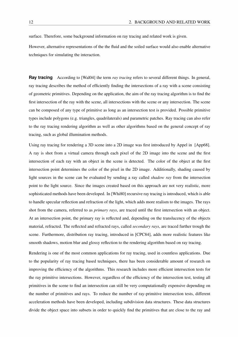
Ray tracing According to [Wal04] the term ray tracing refers to several different things. In general,
ray tracing describes the method of efficiently finding the intersections of a ray with a scene consisting
of geometric primitives. Depending on the application, the aim of the ray tracing algorithm is to find the
first intersection of the ray with the scene, all intersections with the scene or any intersection. The scene
can be composed of any type of primitive as long as an intersection test is provided. Possible primitive
types include polygons (e.g. triangles, quadrilaterals) and parametric patches. Ray tracing can also refer
to the ray tracing rendering algorithm as well as other algorithms based on the general concept of ray
tracing, such as global illumination methods.
Using ray tracing for rendering a 3D scene into a 2D image was first introduced by Appel in [App68].
A ray is shot from a virtual camera through each pixel of the 2D image into the scene and the first
intersection of each ray with an object in the scene is detected. The color of the object at the first
intersection point determines the color of the pixel in the 2D image. Additionally, shading caused by
light sources in the scene can be evaluated by sending a ray called shadow ray from the intersection
point to the light source. Since the images created based on this approach are not very realistic, more
sophisticated methods have been developed. In [Whi80] recursive ray tracing is introduced, which is able
to handle specular reflection and refraction of the light, which adds more realism to the images. The rays
shot from the camera, referred to as primary rays, are traced until the first intersection with an object.
At an intersection point, the primary ray is reflected and, depending on the translucency of the objects
material, refracted. The reflected and refracted rays, called secondary rays, are traced further trough the
scene. Furthermore, distribution ray tracing, introduced in [CPC84], adds more realistic features like
smooth shadows, motion blur and glossy reflection to the rendering algorithm based on ray tracing.
Rendering is one of the most common applications for ray tracing, used in countless applications. Due
to the popularity of ray tracing based techniques, there has been considerable amount of research on
improving the efficiency of the algorithms. This research includes more efficient intersection tests for
the ray primitive intersections. However, regardless of the efficiency of the intersection test, testing all
primitives in the scene to find an intersection can still be very computationally expensive depending on
the number of primitives and rays. To reduce the number of ray-primitive intersection tests, different
acceleration methods have been developed, including subdivision data structures. These data structures
divide the object space into subsets in order to quickly find the primitives that are close to the ray and

2.2. COMPUTER GRAPHICS METHODS 13
therefore more likely to be hit than primitives that are further away. The main concepts of subdivision
data structures are either spatial subdivision or a hierarchical subdivision of the scene.
Hierarchical subdivision is used by so-called bounding volume hierarchies. Primitives are hierarchically
arranged in subsets surrounded by a bounding volume which is usually a box or a sphere. Overlapping
of bounding volumes is permitted. ( [Wal07], [WBS07])
On the contrary, spatial subdivision structures divide the object space into disjoint subsets. These struc-
tures include grids and tree structures.
Tree structures are created by separating the space into subsets using planes. Recursively subdividing
the subsets again leads to a tree structure. Dividing the space into two subsets per division step results in
a binary tree such as a BSP-tree or a kd-tree. ( [IWP08], [Hav02], [WH06]) Dividing the space into four
or eight subsets per step results in tree structures called quadtrees or octrees respectively. ( [BD02])
The efficiency of the acceleration data structures depends on both the technique used to build the structure
and the algorithm applied to traverse through the structure in order to find the intersections with the
primitives ( [Wal04]).
The various acceleration data structures have different advantages and disadvantages and the choice of
data structure depends on the nature of the application. Animated scenes with changes in geometry
require a data structure that can efficiently be rebuild such as grids whereas applications with a huge
number of intersection tests require a data structure that allows for a fast traversal like kd-trees.
According to [Hav00], the most efficient data structure in ray tracing based applications is in most cases
a kd-tree generated based on a surface area heuristic (SAH). Therefore, the SAH based kd-tree is the
acceleration data structure chosen for this project.
2.2.3 Visualization of interaction features
After simulating the interaction between the liquid jets and the soiled surface, the final task is to find a
way to visualize the intersection points and the additional data collected about the characteristics of the
intersection. One approach is to store the intersection points separate from the surface and use primitives
such as spheres for points or arrows for vectors to visualize the data. However, this approach provides
no direct connection between the surface and the collected data.
Intersection points and intersection data can be stored directly with the mesh as well. A common method
for visualizing attributes on a surface is assigning color values to the parameters and displaying these
colors directly on the surface as a false-color representation. Interactively applying color attributes to

14 2. BACKGROUND AND RELATED WORK
a surface is similar to the problem of 3D painting. Attributes can be stored per vertex as in [HH90].
However, this approach requires a high geometric resolution (i.e. a high number of small primitives) in
order to visualize small details. To achieve a resolution for visualizing the attributes that is independent
from the geometric resolution of the mesh, attributes can be stored in a texture that is mapped onto the
mesh instead. Textures can be easily processed and rendered by the GPU and therefore texture mapping
is a very efficient method to store surface attributes. However, mapping the texture image onto the surface
requires a parameterization of the surface. Often, the surface has to be divided into smaller parts that are
parameterized separately, which can lead to discontinuities at the borders of these parts. Furthermore,
mapping usually implicates a distortion of some degree.
To avoid parameterization of the surface, another method has been developed to store surface attributes
such as the color. This method is called an octree texture and is described by Benson and Davis
in [BD02]. Attributes are stored in an octree data structure build around the object. However, octree
textures cannot be processed by the GPU as efficiently as texture maps, yet.
Since the surface representation used in this application is a triangle mesh and triangles can be param-
eterized easily via barycentric coordinates there is no direct need for avoiding parameterization. Yet,
efficient rendering of the intersection data is an important factor. Therefor, texture mapping is applied in
this simulation to store and visualize the intersection data. To highlight the characteristics of texture map-
ping, more background information about the technique is given in the following paragraph, including
an overview of applications of textures.
Texture mapping Texture mapping was first used to create more realistic 3D models by mapping 2D
images containing characteristic color features of the object’s material onto the object’s surface instead
of defining the color for each vertex separately. To map an image onto the 3D model, the model is
required to be homeomorphic to a disc. If the model does not meet this requirement, it can be divided
into multiple segments that are homeomorphic to a disc. These segments are called charts. Segmenting
a model into charts can either be performed manually by the user as in [Ped95], or automatically as
in [MYV93]. [SSGH01] applies a region growing approach for the segmentation.
After dividing the model into charts, each chart needs to be parameterized to create a texture map.
Initially charts had to be convex to apply parameterization algorithms. Therefore the boundary nodes
of the chart were mapped onto the boundary of a disc or square ( [LM98]). The remaining vertices of
the chart were then processed by solving an energy minimization problem. In [HG00] a parametrization
technique was introduced that did not require a convex boundary. Instead an arbitrary boundary shape
was possible.

2.2. COMPUTER GRAPHICS METHODS 15
Each texture map can be handled as a separate texture by the GPU. However, this implies multiple texture
switches for the GPU just to render a single object. Since these texture switches are computationally ex-
pensive, texture atlases have been developed. A texture atlas, introduced by Maillot et. al. in [MYV93],
is a collection of several texture maps in one texture image, which can be processed by the GPU as one
single texture. Packing the texture maps into the texture atlas while making optimal use of texture mem-
ory is a complex challenge known as the bin packing problem. In [SSGH01] the texture maps are packed
according to their bounding box, while [LPRM02] takes the correct boundary of the texture maps into
account.
Due to the fast processing of textures with modern graphics hardware and the independence of the reso-
lution of the texture from the geometric resolution of the object, several other applications have emerged.
These include techniques that improve the appearance of 3D models by adding more realism, such as
bump mapping, displacement mapping or environment mapping.
Textures are also used, for example, for storing global illumination data in so-called light maps ( [RcUCL03]).
Furthermore shadow maps are stored in textures to add shadows to a scene ( [DS03], [DS05]). In addi-
tion to storing previously computed data, textures are used for interactive painting on 3D shapes as well
( [HH90], [IC01]).

16 2. BACKGROUND AND RELATED WORK

17
3 Requirements and implementation
The goal of this project is to simulate the functionality of a CIP system, which means simulating the
interaction between a cleaning liquid and an object that is to be cleaned. This includes representing the
crucial components of the system in the 3D simulation, calculating the intersection of the cleaning liquid
with the soiled object and visualizing the parameters describing the nature of the intersection. Back-
ground information on the algorithms used to achieve this goal has been given in the previous section
(2). The following sections present the Computer Graphics approaches which have been applied in more
detail. If adaptations are necessary to use an algorithm for this application, they are emphasized. Sec-
tion 3.1 illustrates the methods used to represent the basic components of a CIP system in 3-dimensional
space. Section 3.2 then explains in detail the implementation of the interaction between the fluid and
the objects in the simulation. Finally, section 3.3describes the collection and display of the intersection
information.
3.1 3D representation of the CIP system components
As mentioned before, the purpose of the CIP system is to clean the surface of an object by spraying it
with a special fluid. The interaction of the fluid with the soil on the object’s surface determines the result
of the cleaning process. However, not the chemical reaction between the fluid and the soil is relevant in
this simulation, but merely the fact of the fluid reaching the object’s surface. Therefore the important
components of the CIP system that need to be considered for the simulation process can be limited to the
object that is to be cleaned and the spray nozzles. For the simulation of the spray nozzles, a representation
of the fluid and an algorithm for distributing the fluid are required.
3.1.1 Fluid representation
Choosing the ideal form to represent the fluid is a crucial factor in the simulation. As described in chap-
ter 2, the two basic approaches developed by the computer animation community to simulate fluids are
either using a grid to discretize the space of the fluid (Eulerian approach) or defining particles through-
out the whole volume of the fluid (Lagrangian approach). As also mentioned before, both approaches
18 3. REQUIREMENTS AND IMPLEMENTATION
have a downside, which is why hybrid methods have been developed to combine the benefits of both
(e.g. [FF01], [ELF05]). According to [KCC+06], particle based models are more suitable for simulating
complex free surface motion of liquids than grid based methods. Since jets created by a spray nozzle have
a large scale free surface (i.e. the surface between the fluid and the air), a particle based method seems to
be more appropriate. However, both particle and grid based simulations of fluids are very complex and
expensive,according to [GH06], and therefore exceed the limitations of this project. Therefore, a more
simple approach is required. Yet, to receive useful data about the cleaning result the representation needs
to be physically correct to a certain extend. The simplification, however, always causes minor deviation
that should be considered while evaluating the results.
To simplify the representation of the fluid, it is important to analyze the characteristics of the fluid in the
real system. In the CIP system, the fluid is sprayed through different types of spray nozzles, creating
single jets of fluid. By disregarding the impact one jet of fluid has on its neighboring jets, the jets can be
interpreted as independent entities. Based on this constraint, the task is now to represent a single jet of
fluid.
Straight line
The easiest way to do this, is by describing the jet as a straight line. The line represents the trajectory of
the uncoupled fluid particles, the path the particles follow through space.
The position x of the particle at time t is then described by the following equation of motion with no
influence of an external force, where x0 is the starting point of the fluid particles at time t = 0.
~x(t) = ~x0 + ~v · t (3.1)
The velocity vector ~v is defined as ~v = v · ~d, with ~d setting the direction in which the particles move and
v being the particles’ constant velocity.
It should be obvious that a straight line is not a physically correct representation of a jet, since no physical
forces such as gravity or drag are taken into account. Furthermore, physical characteristics of the fluid,
such as the density, the viscosity or the temperature are not taken into account either. However, a straight
line is an ideal starting point, since efficient algorithms for line-object intersection already exist, due
to its similarity to rays in ray tracing applications. These intersection tests are necessary for applying
established ray tracing based algorithms in this simulation. The intersection test and its implementation
are described in more detail in section 3.2.1.

3.1. 3D REPRESENTATION OF THE CIP SYSTEM COMPONENTS 19
Parabola
Since the straight line is a highly simplified representation of a jet, it is necessary to take more physical
forces into consideration and increase the physical correctness of the simulation. By assuming a uniform
gravity, the trajectory of the fluid particles change from a straight line to a parabola. The following
equation describes the trajectory, with ~x(t) being the position of the particle at time t and ~x0 being the
position at t = 0.
~x(t) = ~x0 + ~v · t + ~g · t2 (3.2)
~v corresponds with the velocity vector in equation 3.1 and ~g denotes the acceleration due to gravity in
3D space. Since the y-axis is considered perpendicular to the horizon in this simulation, the y value of
vector ~g is −12g whereas the other two remaining values are both 0. g is the acceleration due to gravity, a
physical constant with the value 9, 81ms2 , which only applies in vertical direction towards the center of the
Earth. Furthermore, ~g contains the factor 12 to ensure that the second derivative of ~x(t) in equation 3.2,
which denotes the acceleration ~a of the particles, is equivalent to the acceleration due to gravity.
~a(t) = x(t) =
0
−g
0
Representing the jet with a parabolic trajectory is still not perfect, since no drag or wind are considered,
as well as other physical characteristics of the fluid, such as pressure or density. Furthermore, the gravi-
tational force field is reduced to a uniform gravity. But the parabola is more physically plausible than a
straight line, at least for particles at lower speed, and at the same time allows for simple intersection and
reflection algorithms. The algorithms applied in this simulation are further described in section 3.2.1.
However, the higher the speed of the particles the more the trajectory resembles a straight line instead
of a parabola. This is where the line representation comes in handy. The simulation of the CIP sys-
tem contains both the line and the parabola representation for the fluid. All algorithms regarding the
intersection of the fluid with the object and the evaluation of intersection data are implemented for both
representations.
3.1.2 Spray nozzle representation
To simulate the functionality of a CIP system correctly, the distribution of the fluid jets in the simulation
has to match the real distribution. Therefore the parameters of the sources of the fluid jets need to be

20 3. REQUIREMENTS AND IMPLEMENTATION
adapted to the parameters of the real spray nozzles. Especially the spray patterns produced by the spray
nozzles should match the original spray patterns. The spray pattern described the image created by
the fluid jets of a source hitting a planar surface perpendicular to the main propagation direction and
is connected to the way, jets are distributed by the nozzle. In real CIP systems, different types of spray
nozzles with different spray patterns are used. Spray nozzles can either be fixed or rotating. Furthermore,
nozzles can be assembled separately or combined to form clusters. Figure 3.1 shows different types of
spray nozzles.
(a) (b) (c)
Figure 3.1: Different nozzle types ( [:2006])
To enable a greater variety of spray tests it is necessary to provide different types of spray nozzles in the
application as well. However, only fixed spray nozzles have been considered so far, since the rotation of
the spray nozzles would increase the complexity of the calculation considerably. Still, rotating nozzles
could be a subject of future work. The spray nozzle types available in the simulation include full cone
spray nozzles, hollow cone spray nozzles and flat fan spray nozzles.
For each spray nozzle there are several parameters to adjust. Parameters all nozzle types have in common
include the position and orientation of the nozzle, the number of jets generated by the nozzle and the
velocity of the fluid. Furthermore, the type of ray (i.e. straight line or parabola) can be selected as well.
There are further parameters for each nozzle type to define the aperture of the nozzle. These parameters
are included in the description of the various nozzle types below.
The general algorithm for generating jets of fluid is similar for all three nozzle types. As described in
section 3.1.1 the jets can be described by equation 3.1 in case the jet is a straight line and by equation 3.2
in case the jet is a parabola. The position ~x0 (i.e. the starting point) is equal for all rays and corresponds
with the position of the spray nozzle. The only value that is different for all rays is the velocity vector
~v. This vector is created by combining the speed v of the fluid particles with a vector ~d describing the
direction of the ray. The speedv can be defined by the user whereas the direction vector ~d is generated

3.1. 3D REPRESENTATION OF THE CIP SYSTEM COMPONENTS 21
(a) (b)
Figure 3.2: (a) The direction vectors ~d of the fluid jets are situated within a defined region. (b) This
region can also be described by a section on the unit sphere surrounding the starting point of
the fluid jets.
randomly according to the following algorithm.
For every ray the direction vector ~d lies within a defined region centered around a vector depicting the
orientation of the nozzle. The size of this region is determined by the type of nozzle and the parameters
set by the user. For every spray nozzle type, this region represents a section of the unit sphere surrounding
the starting point ~x0 of the rays. (see figure 3.2)
The direction vectors of the rays are now created by uniformly sampling this section of the sphere. The
sphere is sampled uniformly by applying Archimedes’ theorem as described in [SB96]. According to
the theorem the lateral surface of a cylinder (without the bases) circumscribed about a sphere is equal to
the surface of the sphere. Furthermore the axial projection of any measurable region on the sphere on
the lateral surface of the cylinder preserves area (see figure 3.3). Therefore, the surface of the sphere can
be sampled uniformly by sampling the surface of the cylinder and projecting the sampled points inwards
onto the sphere.
Since the cylinder is developable, uniform sampling of the cylinder is straightforward. The lateral surface
of the cylinder equals a rectangle of the size 2π × 2. (see figure 3.4)
The rectangle is sampled by generating a uniformly distributed random number for each coordinate (i.e.
θ and y ) within the defined range. The following equations, where ξ1 and ξ2 are random floating point
numbers between 0 and 1, generate samples on the entire rectangle. To limit the sampled region, the
values can be scaled down to the requested size.
θ = 2πξ1 (3.3)
y = (1− 2ξ2) (3.4)
Now the sampled points on the cylinder have to be projected onto the sphere. Since the projection axis

22 3. REQUIREMENTS AND IMPLEMENTATION
Figure 3.3: According to [SB96], the axial projection of a region on a sphere onto the lateral surface of
a cylinder circumscribed about the sphere preserves area. Therefore the marked region (red)
on the sphere has the same area as the region on the cylinder.
!
!
Figure 3.4: The lateral surface of the cylinder equals a rectangle of the size 2π × 2. To generate the
direction vectors, only a small part of the rectangle is uniformly sampled.

3.1. 3D REPRESENTATION OF THE CIP SYSTEM COMPONENTS 23
is perpendicular to the y-axis, the y value remains unchanged. The x and z values of the samples are
modified according to the following equation.
x = cos θ√
1− y2 (3.5)
z = sin θ√
1− y2 (3.6)
To obtain different spray patterns for the different nozzle types, the sampled region on the cylinder needs
to be adjusted. The spray patterns and sampled regions for each nozzle type will be described in the
following paragraphs.
Apart from the uniform sampling described, there are alternative algorithms for generating the distribu-
tion of fluid jets. A uniform sampling of the sphere could also be achieved, by subdividing geometric
objects (e.g. icosahedron or octahedron) and placing the vertices on the sphere. Furthermore, other
distributions could be used apart from uniform distributions (e.g. Poisson distribution). However, the
advantage of the algorithm used here is the fact, that the section on the sphere that needs to be sampled
can be adjusted very easily, enabling the representation of different spray nozzle types with only small
variations to the same algorithm. Sampling the sphere through subdividing another object would require
more complex methods to select the samples that lie in the region that needs to be sampled. Still, the
current sampling as described before, could be improved, for example, by stratification. ( [SB96])
Type 1 - Full cone spray nozzle The full cone spray nozzle sprays the fluid jets in the shape of a
cone. The jets are uniformly distributed throughout the entire cone. The size of the cone is determined
by the aperture angle α set by the user. The resulting spray pattern matches a filled circle. To achieve a
circular spray pattern, the sampled region on the cylinder is set to a rectangle of size θ × y, with θ and y
depending on the aperture angle α (see figure 3.5).
θ =α · π180
(1− 2ξ1) (3.7)
y = 2 sin θ(1− 2ξ2) (3.8)
After projecting the sampled points onto the sphere, all points outside a circle of radius sin θ around
the center of the cone are dismissed, to ensure a circular shape. This is tested by applying Pythagoras’
theorem. From the position ~x0, the generated direction vectors ~d and the velocity v, new rays (i.e. lines
or parabolas) are created.

24 3. REQUIREMENTS AND IMPLEMENTATION
(a) (b)
Figure 3.5: Full cone spray nozzle: (a) the spray pattern of this nozzle type forms a filled circle. (b) This
spray pattern is achieved by uniformly sampling a square on the cylinder and dismissing all
samples that are outside the circle.
(a) (b)
Figure 3.6: Hollow cone spray nozzle: (a) the spray pattern of this nozzle type forms an unfilled cir-
cle. (b) This spray pattern is achieved by uniformly sampling a square on the cylinder and
dismissing all samples that are outside the outer circle or inside the inner circle.
Type 2 - Hollow cone spray nozzle Similar to type 1 the hollow cone spray nozzles create jets of
fluid in the shape of a cone. However, the jets are not distributed throughout the entire cone. They are
only located close to the boundary of the cone. This leads to a spray pattern that is similar to an unfilled
circle. The width of the band filled with fluid jets can be determined by the user by giving the percentage
of the aperture angle that is supposed to be empty (see figure 3.6).
The direction vectors ~d are created similar to the vectors of type 1. However, points on the sphere, which
are inside the inner cone defined by the percentage, are dismissed.
Type 3 - Flat fan spray nozzle Unlike types 1 and 2, flat fan spray nozzles do not create a circular
spray pattern. Instead spray patterns about the shape of a rectangle are created. This is achieved by
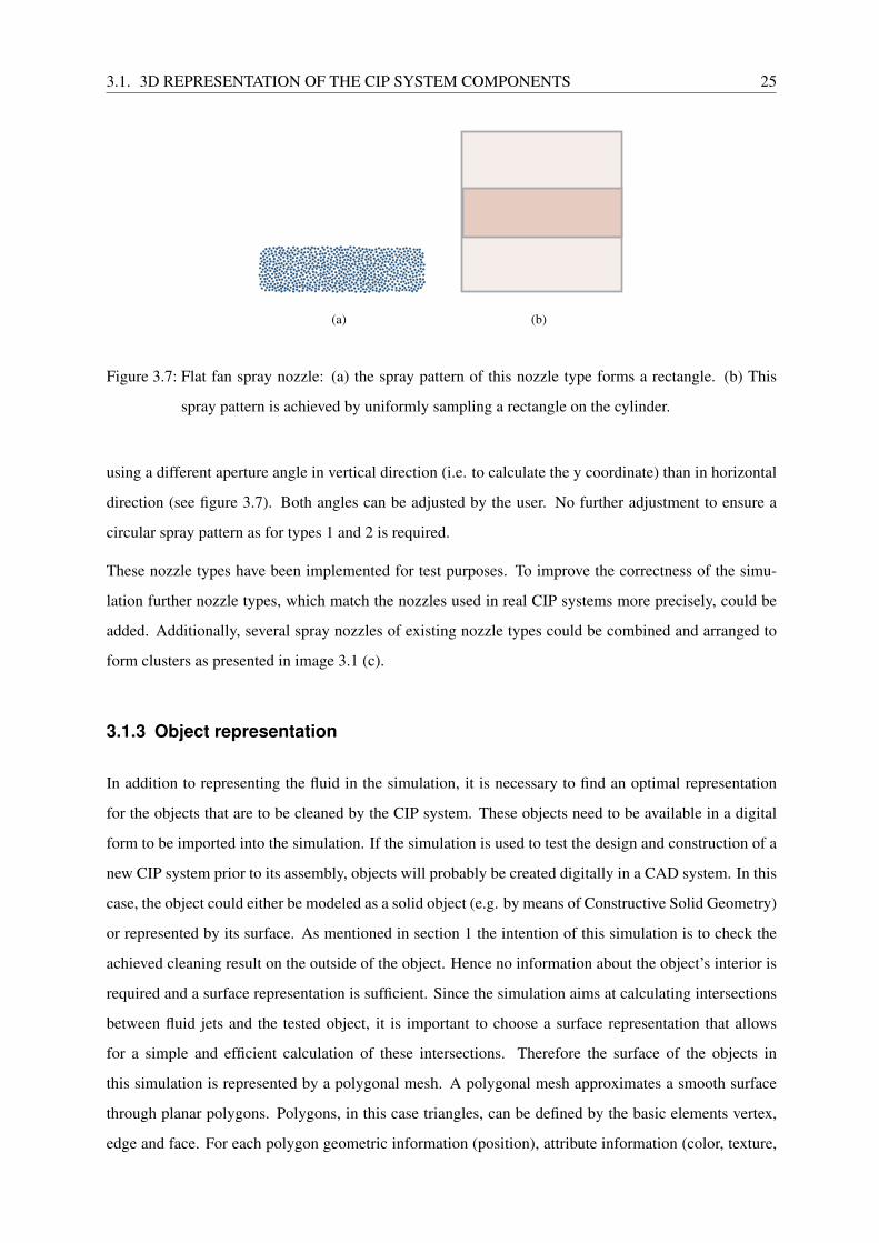
3.1. 3D REPRESENTATION OF THE CIP SYSTEM COMPONENTS 25
(a) (b)
Figure 3.7: Flat fan spray nozzle: (a) the spray pattern of this nozzle type forms a rectangle. (b) This
spray pattern is achieved by uniformly sampling a rectangle on the cylinder.
using a different aperture angle in vertical direction (i.e. to calculate the y coordinate) than in horizontal
direction (see figure 3.7). Both angles can be adjusted by the user. No further adjustment to ensure a
circular spray pattern as for types 1 and 2 is required.
These nozzle types have been implemented for test purposes. To improve the correctness of the simu-
lation further nozzle types, which match the nozzles used in real CIP systems more precisely, could be
added. Additionally, several spray nozzles of existing nozzle types could be combined and arranged to
form clusters as presented in image 3.1 (c).
3.1.3 Object representation
In addition to representing the fluid in the simulation, it is necessary to find an optimal representation
for the objects that are to be cleaned by the CIP system. These objects need to be available in a digital
form to be imported into the simulation. If the simulation is used to test the design and construction of a
new CIP system prior to its assembly, objects will probably be created digitally in a CAD system. In this
case, the object could either be modeled as a solid object (e.g. by means of Constructive Solid Geometry)
or represented by its surface. As mentioned in section 1 the intention of this simulation is to check the
achieved cleaning result on the outside of the object. Hence no information about the object’s interior is
required and a surface representation is sufficient. Since the simulation aims at calculating intersections
between fluid jets and the tested object, it is important to choose a surface representation that allows
for a simple and efficient calculation of these intersections. Therefore the surface of the objects in
this simulation is represented by a polygonal mesh. A polygonal mesh approximates a smooth surface
through planar polygons. Polygons, in this case triangles, can be defined by the basic elements vertex,
edge and face. For each polygon geometric information (position), attribute information (color, texture,

26 3. REQUIREMENTS AND IMPLEMENTATION
etc.) and topological information (adjacency, connectivity) can be stored with these basic elements.
The triangle mesh is the optimal method for representing the surface of the object, since it meets all the
main requirements. First, the surface representation needs to enable a fast and efficient intersection test
with the fluid jets. The intersections of both a straight line and a parabola with a triangle are considerably
easy to calculate and a triangle mesh also enables the use of acceleration data structures as mentioned
in section 2 to reduce the computational costs. Detailed information about the intersection is given in
section 3.2.1. Second, the results of the intersection test (e.g. parameters such as the particle speed or the
intersection angle) are required to be stored and displayed on the surface. As mentioned in section 2, the
data can be visualized by mapping a 2D texture image onto the surface and storing the data in this image.
To map the image onto the surface, the surface needs to be parameterised to find the equivalent point
in the image for each point on the surface. However, the image can only be mapped onto the surface
without distortion, if the surface is homeomorphic to a disc. Otherwise, the surface needs to be split
into smaller parts that are embedded into the texture separately. The separate parts can then be packed
into one texture atlas. The advantage of a triangle mesh is, that triangles can easily be parameterised
via barycentric coordinates, which is necessary to map the texture onto the surface. More details about
barycentric coordinates are given in section 3.2.1. Finally, the surface needs to be rendered. Triangle
meshes can be rendered very fast, since triangles can be directly processed by the GPU.
The simulation contains two different data structures for storing the topological information of the trian-
gle mesh according to the current processing step. During the generation of the texture atlas, described
in more detail in section 3.3, connectivity information is required to divide the surface into smaller parts
that can be embedded in the texture. Therefore, a triangle mesh with a half-edge data structure is used.
The triangles are described by the three basic elements mentioned before. Each edge is described by a
pair of edges (so-called half-edges) with opposite orientation. Since an edge connects two faces, each
half-edge is associated with one face. A link to this face is stored with each half-edge as well as a link to
the other half-edge in the pair (see figure 3.8 (a)).
All half-edges surrounding the same face form a linked list. The orientation of this list can either be
clockwise or anti-clockwise, but has to be consistent throughout the entire mesh. For every half-edge in
the list, a link to the next half-edge according to its orientation is stored. In some application the previous
half-edge is stored as well. However, this is not mandatory (see figure 3.8 (b)).
Additionally, a link to one of the vertices incident to the half-edge is stored as well. In this case a link to
the origin of the half-edge is stored with every half-edge (see figure 3.8 (c)).
This leads to the following data structure for half-edges, which also contains attribute information (see
figure 3.10). Most of the topological information is stored with the half-edges. The data structure for the

3.1. 3D REPRESENTATION OF THE CIP SYSTEM COMPONENTS 27
(a) (b) (c)
Figure 3.8: Topological information stored per half-edge: (a) Each half-edge is linked to the half-edge
with opposite orientation that is associated with the same edge. Furthermore, a half-edge is
linked to the face it is incident to. (b) All half-edges associated with the same face form a
linked list, with each half-edge pointing towards the origin of the following half-edge. For
each half-edge, a link to the next half-edge is stored. (c) Finally, a link to the vertex forming
the origin of the half-edge is stored.
(a) (b)
Figure 3.9: Topological information stored per (a) vertex and (b) face: Each vertex as well as each face
is linked to one of the incident half-edges. A vertex is linked to a half-edge originating from
this vertex, whereas a face is linked to one of the half-edges forming the linked list around
this face.

28 3. REQUIREMENTS AND IMPLEMENTATION
vertices now only contains the geometrical information for each vertex and a link to one of the half-edges
that originate from this vertex. The data structure for the faces of the mesh only contains a link to one of
the half-edges surrounding the face, as well (see figure 3.9).
Figure 3.10: This figure shows the data structures used to store the connectivity information.
During the calculation of the spray process, described in section 3.2, no topological information about
the triangle mesh is needed since all triangles are processed separately. Thus, a simplified representation
of the triangle mesh is used. Each triangle only stores geometric information about its three vertices
and attribute information like normals and texture coordinates. Usually, a triangle is represented by its
three vertices. Here, only the position of one of the three vertices is stored directly. In addition, two
vectors defining the two edges incident to this vertex are stored as well. (see figure 3.11) These vectors
are used for testing the intersection of a ray with the triangle as described in section 3.2. By storing these
vertices directly instead of calculating them when necessary, the performance of the intersection test can
be improved. With one vertex and two edges, the triangle is defined completely, since the missing values
can be calculated from the values stored. No information about neighboring triangles is stored. The
entire mesh is represented by a list of its triangles.
Both data structures have advantages and disadvantages. The half-edge data structure is more sophis-
ticated, since it enables all adjacency queries, such as loops around a face or a vertex. Furthermore,
attributes can be stored per half-edge instead of only per vertex. However, the half-edge data structure
can only be used for manifold meshes. A mesh is considered manifold, if every boundary edge is inci-
dent to exactly one face and every non-boundary edge is incident to exactly two faces. In addition, no

3.1. 3D REPRESENTATION OF THE CIP SYSTEM COMPONENTS 29
! "
#
Figure 3.11: The triangle mesh consist of single triangles, each storing one vertex (A) and two vectors (b
and c) as geometric information.
t-junctions, internal polygons or breaks in the mesh are allowed. Due to the additional topological infor-
mation stored, the half-edge data structure requires more storage space than the simplified triangle mesh.
On the other hand, the simple triangle mesh does not enable adjacency queries, since no topological
information is stored.
At the current state of development of the simulation, both the half-edge data structure and the simplified
triangle mesh are created by reading the geometric information from an OBJ file. In the future, other file
formats closer related to CAD systems could be supported as well.
3.1.4 Transformation
The positions of all triangle vertices are stored in coordinates referring to the local coordinate system
of the triangle mesh. Additionally, all location and direction parameters of the fluid jets generated by
a spray nozzle refer to the local coordinate system of the nozzle.(see figure 3.12) For interaction of the
fluid jets with the triangles, which is described in section 3.2 a coordinate transformation is required, to
transform all coordinates into the same system.

30 3. REQUIREMENTS AND IMPLEMENTATION
Figure 3.12: Transformation: The scene is arranged in a global coordinate system. However, each com-
ponent (i.e. the spray nozzles and the cleaning object) is stored in coordinates referring
to a local coordinate system. To calculate interaction between the components, they need
to be transform into the same coordinate system via a transformation matrix. All compo-
nents can either be transformed into the global coordinate system or one component can be
transformed from its own local system into the local system of the component it interacts
with.
3.2. INTERACTION BETWEEN FLUID AND OBJECTS 31
3.2 Interaction between fluid and objects
The interaction between the fluid sprayed from the nozzles and the object that is to be cleaned forms the
crucial factor of the simulation since it represents the main functionality of the cleaning system. The fluid
jets are sprayed into the scene and goal is to find the points where the jets reach the surface of the object.
As illustrated in section 3.1, the fluid jets can be represented in a simplified manner as independent
rays in the shape of a straight line or a parabola. This representation, more precisely the straight line
representation, bears resemblance to the general representation of light rays used in many illumination
applications. Light rays, examined on a macroscopic level, are assumed to propagate linearly and can
therefore be represented as straight lines.
Additionally, the problem of a fluid reaching the surface of an object without obstacles appears similar to
the visibility problem found in rendering and illumination applications. A point is visible from another
point in space if the line between these point does not intersect any obstacles on the way. The visibility
problem equals the task of finding the first intersection of a ray with an object in the general concept of
ray tracing described in section 2.
This analogy between the interaction of the fluid and an object and the concept of ray tracing, on the basis
of the close relation of the fluid representation to the representation of light rays and the similarity of the
overall problem, allows for the application of established ray tracing algorithms in order to simulate the
cleaning systems functionality.
In recursive ray tracing, optical phenomena like reflection and refraction are handled by tracing the rays
further after the first intersection with an object. A jet of fluid which hits a surface can be reflected in a
similar way, though based on the characteristics of the fluid. Refraction, however, is not relevant in this
context, since the materials used in CIP applications are mainly impermeable to liquids.
Similar to other ray tracing based applications, the number of intersection tests between fluid jets and
the geometric primitives can be very high. Complex objects are very likely to consist of a huge number
of primitives (i.e. triangles) and a reasonably realistic simulation of the spray nozzles requires a vast
amount of fluid jets as well. To reduce computation time and avoid the intersection test for each fluid
jet with each triangle, acceleration methods are required. An overview of acceleration data structures
commonly used in ray tracing based applications is given in section 2.
The following sections describes in detail the calculation of the intersection of the jets of fluid with the
object that is to be cleaned. At first, the calculation of the actual intersection is presented, followed by
an introduction to the acceleration method applied to reduce the number of intersection tests. Finally,
the last subsection takes a look at the tracing of jets reflected at the object’s surface. Due to the analogy

32 3. REQUIREMENTS AND IMPLEMENTATION
to ray tracing the jets will generally be referred to as rays. However, if an algorithm requires a distinc-
tion between the two different forms of fluid representation (i.e. straight line or parabola), this will be
highlighted and each representation will be dealt with separately.
3.2.1 Ray-object intersection
Finding the intersection of a ray with an object requires a preferably efficient intersection test for the
primitives the object is constructed from. As described in section 3.1.3 the objects in this application
consist of planar triangles. To allow an object intersection test for both the straight line representation
and the parabola representation of the jets of fluid, triangle intersection tests for both representations are
required.
3.2.1.1 Line-triangle intersection
Since line-triangle intersections are quite common in many computer graphics applications, such as
ray tracing, there has been a considerable amount of research, which lead to a number of different ap-
proaches.
The first step most of these approaches have in common is testing if the line intersects the plane the
triangle lies in. As illustrated in section 3.1, the line can be described by the following equation, where
~x0 is the starting point of the line and ~v is the velocity of the particles.
~x(t) = ~x0 + t · ~v (3.9)
A plane is defined by equation 3.10, which holds for every point ~x that lies in the plane. ~n is the normal
of the plane and d is defined as the distance of the plane from the origin of the coordinate system.
~n · ~x− d = 0 (3.10)
To find the plane the triangle lies in, the normal ~n and the distance d can be derived from the vertices ~v0,
~v2 and ~v1 of the triangle.
~n =(~v1 − ~v0)× (~v2 − ~v0)‖(~v1 − ~v0)× (~v2 − ~v0)‖
d = ~n · ~v0

3.2. INTERACTION BETWEEN FLUID AND OBJECTS 33
Figure 3.13: A triangle can be defined as the space where three half spaces overlap. If a point lies in all
three half spaces, it lies within the triangle.
If the line does not intersect the plane, there is also no chance of intersecting the triangle and no fur-
ther calculation is required. If, however, the line does intersect the plane, a further test is necessary to
determine whether the intersection point lies within the triangle.
One way to test if the point is inside the triangle is to define the triangle as the intersection of three half
spaces and test whether the point is in all three half spaces (see figure 3.13). ( [Mar03])
Another approach calculates the barycentric coordinates instead to determine whether the intersection
point lies inside the triangle (see figure 3.14).
!
"
"#
"$ "%
&'!(")
Figure 3.14: Barycentric coordinates: A point ~x lies within the triangle, if the barycentric coordinates u
and v are ≥ 0 and u + v ≤ 1.
x(u, v) = (1− u− v) · ~v0 + u · ~v1 + v · ~v2 (3.11)
If both barycentric coordinates u and v are ≥ 0 and u + v ≤ 1, p is inside the triangle. u and v can
be stored and reused later on during the texture mapping for interpolation purposes, which makes the
second approach more interesting in this case.
However, a third approach exists, which requires less storage then the previous methods and also calcu-

34 3. REQUIREMENTS AND IMPLEMENTATION
lates the barycentric coordinates necessary for interpolation in the process. This method, described in
[MT97] , avoids the intersection test with the plane by not combining equation 3.9 with equation 3.10
but with equation 3.11 instead.
~x0 + ~v · t = (1− u− v) · ~v0 + u · ~v1 + v · ~v2 (3.12)
Rearranging equation 3.12 leads to the following equation with the unknown parameters t,u and v.
[−~v,~v1 − ~v0, ~v2 − ~v0] ·
t
u
v
= ~x0 − ~v (3.13)
After substituting ~e1 for (~v1 − ~v0), ~e2 for (~v2 − ~v0) and ~e3 for (~x0 − ~v0) and applying Cramer’s rule
equation 3.13 can be written as follows, where |A,B, C| = −(A× C) ·B = −(C ×B) ·A:
t
u
v
=1
| − ~v,~e1, ~e2|·
|~e3, ~e1, ~e2|
| − ~v,~e3, ~e2|
| − ~v,~e1, ~e3|
(3.14)
Substituting ~p for (~v × ~e2) and ~q for (~e3 × ~e1) leads to the final equation.
t
u
v
=1
~p · ~e1·
~q · ~e2
~p · ~e3
~q · ~v
(3.15)
3.2.1.2 Parabola-triangle intersection
The intersection of the parabola with the triangle is tested by calculating the intersection point(s) of the
parabola with the plane the triangle lies in first and afterwards testing if the point lies inside the triangle.
The plane of the triangle is defined by one vertex ~p and the face normal ~n of the triangle.
0 = (~x− ~p) · ~n (3.16)
As described in section 3.1.1 the parabola is defined by a quadratic equation. The combination of equa-
tions 3.2 and 3.16 leads to the following quadratic equation.

3.2. INTERACTION BETWEEN FLUID AND OBJECTS 35
0 = (~g · ~n)t2 + (~v · ~n)t + ((~x0 − ~p) · ~n) (3.17)
The equation can have 0,1 or 2 solutions. The different cases can be distinguished by the discriminant of
the equation. The discriminant disc is defined as follows:
disc = (~v · ~n)2 − 4(~g · ~n)((~x0 − ~p) · ~n)
If disc < 0, equation 3.17 has no solution and the parabola does not intersect the plane. If disc = 0,
there is exactly one solution.
t1/2 = − ~v · ~n2(~g · ~n)
In this case the parabola touches the plane.
If disc > 0, there are two solutions and the parabola intersects the plane twice.
t1 =−(~v · ~n)− sgn(~v · ~n) ·
√disc
2(~g · ~n)
t2 =(~x0 − ~p) · ~n(~g · ~n) · t1
This is true, unless the plane is perpendicular to the x-z-plane. In this case (~g · ~n) = 0 and equation 3.17
is reduced to a linear equation.
After the intersection points have been calculated, it has to be determined whether at least one point is
inside the triangle. A linear system of equations is constructed to find the barycentric coordinates. If
the parabola intersects the triangle twice, the intersection that is closest to the origin of the parabola is
stored.
3.2.2 Acceleration methods
Since the ray nozzles are likely to produce a large number of fluid jets and complex objects or scenes
consist of thousands of primitives that need to be tested for intersection with each ray, visibility tests tend
to be very expensive and time consuming. Therefore an acceleration method is required that reduces
the number of intersection tests. An overview of possible acceleration methods is given in section 2.
According to a comparison of different spatial subdivision structures conducted by V. Havran in [Hav00]

36 3. REQUIREMENTS AND IMPLEMENTATION
the most efficient method is a kd-tree with a surface area heuristic (SAH). Therefore, this method has
been implemented to reduce the number of intersection tests.
The kd tree is a special kind of Binary Space Partitioning (BSP) tree. A BSP tree is a data structure that
subdivides the space of an object, defined by a number of vertices, into smaller subspaces by separating
the vertices spatially through an arbitrarily oriented split plane. Subspaces can be split again by a new
split plane always creating two new half spaces. Recursively splitting the spaces into two half spaces
leads to a binary tree structure. The kd tree differs from the BSP tree as only split planes perpendicular to
one of the coordinate axes are allowed. (see figures 3.15 and 3.16) This reduces the data that needs to be
stored for each split plane to an index of the split axis and the split position along this axis. Furthermore
axis aligned split planes simplify the construction and intersection of the tree. The construction of the kd
tree, including the selection of the next split axis and the next split position on this axis, are described in
the following section. After that, the traversal through the tree in case of an intersection is described in
section 3.2.2.2.
!
"
(a)
!
"
(b)
!
"
(c)
Figure 3.15: Kd-tree: The space of the triangles (in 2D) is split recursively to build a kd tree. (a) The first
split axis is perpendicular to the x-axis, separating the space into two subspaces. (b) Each
subspace is split again, this time along the y-axis, generating a total of four subspaces. (c)
Finally, all subspaces are split again along the x-axis.
3.2.2.1 Kd-tree construction
To divide the space of the cleaning object into subsections and build a tree structure, the split planes need
to be selected. Different criteria for selecting the next split axis and split position exist.
Normally, any position along the split axis can be used to position the split plane. However, often certain
positions are preferred, such as the spatial mean or a position that divides the elements (e.g. vertices,
triangles, etc.) into two sets with the same amount of elements in each set. Furthermore, the positions of
the vertices can be used as potential split positions. For the SAH based kd-tree, only the vertex positions
are considered as potential split positions and the surface area heuristic is calculated to find the optimal

3.2. INTERACTION BETWEEN FLUID AND OBJECTS 37
!"
#$%&'(
)"
(a)
!"#$%& !"#$%&
'( '()( )(
(b)
!"#$%&
'( )(
!"#$%&
'( )(
!"#$%&
'( )(
!"#$%&
'( )(
(c)
Figure 3.16: Kd-tree: The kd tree is constructed according to the splits illustrated in figure 3.15 and the
triangles are are assigned to the nodes of the kd tree according to their position.
position. While arbitrary positions can be used as split positions, to separate vertices for example, they
would have no effect on the SAH calculated for the triangles and therefore do not have to be considered.
(see figure 3.17)
(a) (b) (c)
Figure 3.17: Split positions: (a) To separate vertices, arbitrary positions can be selected as split positions.
Potential split positions are often the vertex positions, the spatial median (blue) or the po-
sition dividing the vertices into two sets of the same size (red). (b) Triangles can also be
separated at the spatial mean or divided into two sets of equal size. If a triangle overlaps
the split plane, it is assigned to both sides of the plane. (c) For the SAH kd-tree only the
positions of the triangles’ vertices are taken into account as potential split positions.
To build the kd-tree, all triangles are assigned to the root node first. After the optimal or next split
position has been found, the object is split along the plane and a child node is created for each subset.
All triangles are assigned to either of the child nodes or both. Each child node is then split again. This
algorithm continues recursively for each new child node, creating a tree structure, until a predefined
termination criterion is met. Possible termination criteria include a maximum tree depth or a minimum
number of primitives per node. A combination of several termination criteria can be applied as well.

38 3. REQUIREMENTS AND IMPLEMENTATION
The CIP system simulation contains two different approaches to selecting the next split plane, a naive
approach and the SAH approach described by Havran.
Naive kd-tree To generate the naive kd-tree, an axis-aligned bounding box is constructed around the
vertices of the root node. The dimension of the bounding box along each axis is calculated and the
greatest is selected to appoint the new split axis. The new split position along this axis is then defined
as the spatial median of the vertices. After the split plane is defined by the split axis and position, all
triangles forming the surface of the cleaning object need to be assigned to one or both sides of the plane.
If a triangle lies within the split plane or stretches across the plane, it is assigned to both sides. Otherwise
it is assigned to either of the sides according to its position. After assigning the triangle to a side of the
plane, a new child node is created for each side. The termination criteria determine whether the new
node is an inner node, which can be split further, or a leaf node. For the naive kd-tree the criteria for
termination are a maximum tree depth and a minimum number of triangles per node. Whichever criteria
is met first terminates the splitting of the node. If the termination criteria are not met, yet, the algorithm
described is repeated for each child node. In the completed kd-tree, triangles are only stored in the leaf
nodes, to save memory space.
SAH kd-tree Building a kd-tree with a surface area heuristic (SAH) leads to a tree structure that
allows faster traversal to detect an intersection than the naive kd-tree. The main difference lies in the
selection of the split planes. To find the optimal split position, a cost model is used which estimates
the costs of traversing through the tree and testing for intersection with the primitives. All positions
of vertices of an object count as potential split positions. To determine the optimal split position, all
potential split positions along all three axes are collected. The following image shows the options for a
new split position. For each position the number of primitives to the left and right of the split plane and
the number of primitives parallel to the split plane are stored. To reduce the number of cost calculations,
the list of potential split positions is reduced by eliminating duplicate entries.
After finding the potential split positions, the costs for each split are estimated by applying the surface
area heuristic. This cost model is based on geometric probability, which means the probability with
which the bounding box of a child node in the tree is hit by a ray in case the box of the parent node is hit
as well.(see figure 3.18) This probability p can be determined as follows:
pchild|parent =SurfaceArea(BoundingBox(child))
SurfaceArea(BoundingBox(parent))(3.18)
The complete cost model for splitting a node at a selected position is then calculated by equation 3.19.

3.2. INTERACTION BETWEEN FLUID AND OBJECTS 39
!"#$%&
'()*+
Figure 3.18: Geometric probability: The ratio of the surface area of the child node’s bounding box to the
surface area of the parent node’s bounding box estimates the probability for the ray to hit
the child node in case of an intersection with the parent node.
pleftchild and prightchild denote the probability for a ray to hit the left and right child node respectively,
as defined by equation 3.18, and nleft and nright denote the number of primitives on the left or right
side of the split plane. C_TRAV ERSE and C_INTERSECT are estimated costs for traversing
through the tree from the parent node to the child node and the intersection test with the primitives of
the child node, respectively. Both parameters are set to constant values, with C_TRAV ERSE = 3 and
C_INTERSECT = 4.
costsplit = C_TRAV ERSE + C_INTERSECT · (pleftchild · nleft + prightchild · nright) (3.19)
The split position causing the lowest cost in case of a split is selected as the optimal split position.
However, if the costs for splitting the node at the optimal split position are higher than the costs for
keeping the node a leaf node, no split is performed. The costs for keeping the parent node a leaf are
determined by the number of primitives of the parent node nparent that need to be tested for intersection.
costleaf = C_INTERSECT · nparent (3.20)
In addition to the costs described in equation 3.20, the maximum depth of the tree and the minimum
number of primitives per node are termination criteria as well. Similar to the naive kd-tree, the child
nodes of the SAH kd-tree are split again until a termination criterion is met. Also similar to the naive
approach, triangle positions are only stored in the leaf nodes to save memory space. Compared to the
naive kd-tree, the construction of the SAH kd-tree requires more computation due to the estimation of
the costs for each potential split position. However, the SAh kd-tree allows for a faster traversal through
the tree to test for intersection of the rays with the object.

40 3. REQUIREMENTS AND IMPLEMENTATION
3.2.2.2 Kd-tree traversal
The traversal algorithm applied here is similar to the algorithm TABrec described in [Hav00]. An adapted
version is used to detect an intersection of the parabola with the object, while the original algorithm can
be used to detect the intersection of the straight line with the object.
Traversal with straight line The first step of testing for intersection of the straight line with the
kd-tree is detecting whether the line hits the object at all. An efficient way to do this is by constructing
an axis-aligned bounding box around the entire object and testing the box for intersection with the line.
The line-box intersection test is described in more detail in section 3.2.2.3. If the line does not intersect
the bounding box, it is also impossible for the line to intersect the object. If, however, the line does
intersect the box, further traversal through the kd-tree is necessary to locate the first intersection of the
line with the object. The parameters tentry and texit where the line enters and leaves the bounding box,
respectively, and the parameter tsplit where the line intersects the split plane that divides the root node
into its two child nodes are used to determine the next traversal steps (see figures 3.19 and 3.20). If tentry,
the point where the line enters the box, has a value < 0, the starting point (i.e. where t = 0) lies within
the box. In this case the entry point is not valid and tentry is set to 0. The values of the parameters tentry,
texit and tsplit specify whether the line intersects only the left child node, only the right child node or
both child nodes. If only one child node is intersected, only this node needs to be tested further to detect
an intersection with the object. If both child nodes are intersected by the line, the parameters also specify
the order in which the child nodes are intersected. The child node intersected first is also the first to be
tested for intersection, since this node is more likely to contain the first intersection of the line with the
object. The second child node is kept on a stack in case no intersection is found in the first child node.
To test a child node for intersection a distinction is drawn between inner nodes and leaf nodes. If the
child node is an inner node, the same traversal step described before is repeated for the child node. If ,on
the other hand, the child node is a leaf node, all primitives (i.e. the triangles) belonging to the leaf node
are tested for intersection as described in section 3.2.1.1. If an intersection with a primitive is detected,
the algorithm terminates, since only the first intersection with the object is important.
Traversal with parabola Similar to the traversal of the kd-tree with a straight line the first step of
testing for intersection of the parabola with the kd-tree is detecting whether the parabola hits the object at
all by testing for intersection with the bounding box of the entire object. The parabola-box intersection
test is described in section 3.2.2.3. Unlike the straight line, the parabola can enter and leave the box
twice. This increases the number of cases that need to be distinguished. As illustrated in figure 3.21 the

3.2. INTERACTION BETWEEN FLUID AND OBJECTS 41
!"#!$%
!"&'!
!()*'!
! "#!$%
!"&'!
!()*'!
! "#!$%
!"&'!
!()*'!
Figure 3.19: The line enters the bounding box at tentry, intersects the splitting plane at tsplit, and leaves
the box at texit, intersecting only the left child node, only the right child node or both.
!"#!$%
!"&'!
!()*'!+,
!"#!$%
!"&'!
!()*'!
-,
Figure 3.20: If the line intersects both child nodes, the parameters tentry, texit and tsplit determine the
order in which they are intersected. The child that is intersected first, is also the one that is
first tested for further intersection, since it is more likely to find the first intersection with a
triangle in this node.

42 3. REQUIREMENTS AND IMPLEMENTATION
parabola can intersect only the left child node, only the right child node, the left before the right child
node or the right before the left child node. Additionally the parabola can also intersect the left child
node followed by the right child node before intersecting the left child node again (see figure 3.22). In
the same way the parabola can intersect the right child node twice, if the parabola enters the bounding
box from a different direction. In these two cases the parabola intersects the split plane twice, splitting
the parabola into three sections. Each segment is tested for intersection with the respective child node
separately, keeping the order in which the parabola intersects the child nodes.(see figure 3.23) All child
nodes are again either inner nodes or leaf nodes. In case of an inner node the algorithm is repeated for
the child node exactly as described before. In case of a leaf node, all primitives belonging to the leaf
node are tested for intersection with the parabola according to the algorithm explained in section 3.2.1.2.
Similar to the intersection with a straight line, the traversal algorithm terminates, when an intersection
with a primitive is detected.
!"#!$%!"&'!
!()*'!! "#!$%
!"&'! !()*'! ! "#!$%
!"&'!
!()*'!
Figure 3.21: The parabola enters the bounding box at tentry, intersects the splitting plane at tsplit, and
leaves the box at texit, intersecting only the left child node, only the right child node or both.
!"#!$%
!"&'!
!()*'!+,!()*'!+-
!"#!$%+, !"&'!+-
!()*'!+, !()*'!+-
!"&'!+, !"#!$%+-
Figure 3.22: The parabola intersects the splitting plane twice (at tsplit1 and tsplit2) and intersects both
child nodes. The child nodes can also be intersected twice by the parabola.

3.2. INTERACTION BETWEEN FLUID AND OBJECTS 43
!"#!$%
!"&'!
!()*'!+,!()*'!+-,.
!"#!$%
!"&'!
!()*'!+,!()*'!+-
-.
!"#!$%
!"&'!
!()*'!+,!()*'!+-
/.
Figure 3.23: The parabola intersects the splitting plane twice (at tsplit1 and tsplit2) and intersects both
child nodes. The order in which the child nodes are tested is determined by the parameters.
If a parabola intersects a node twice, the node is tested for intersection with the parabola
twice, each time with the respective section of the parabola.
3.2.2.3 Ray-box intersection
For the fast traversal of the kd tree, an efficient algorithm for ray - bounding box intersection is required.
Since the rays can either be straight lines or parabolas, the intersection test needs to be adapted to both
representations.
Line-box intersection The straight line representation of a ray is very common in ray tracing algo-
rithms. Therefore, very efficient algorithms for line-box intersection have been developed. The algorithm
applied here is described in [WBMS05].
The axis aligned bounding box is defined by six axis aligned planes. The vertices mark the points where
three of these planes intersect. The vertex closest to the origin is the minimum of the box, the vertex with
the longest distance the maximum (see figure 3.24).
!"#
!$%
%
&
'
Figure 3.24: The axis aligned bounding box, defined by the corner points min and max.
Since the planes are axis aligned, the normals of the planes are straightforward. With the minimum and

44 3. REQUIREMENTS AND IMPLEMENTATION
maximum of the bounding box and the normals, each plane can be defined by its normal ~n and a point ~p
that lies in the plane.
(~x− ~p) · ~n = 0 (3.21)
For each plane, the intersection with the ray is calculated. ~x0 is the origin of the ray and ~v the ray’s
velocity as defined in equation 3.1.
t =(~p− ~x0) · ~n
~v · ~n(3.22)
Since the planes are axis aligned, the planes’ normals are 0 for two coordinates and 1 for the remaining
coordinate, which reduces equation 3.22.
For planes perpendicular to the x-axis the equation is reduced to:
t = (px − x0x) · vinvx
vinvx is used to avoid the division and is defined as 1vx
. The reduced equations for planes perpendicular
to the y- or z-axis are defined accordingly.
At first, the intersection parameter t for both planes perpendicular to the x-axis is calculated. The smaller
value is denoted as txmin , the greater value as txmax . The same is repeated for the two planes perpen-
dicular to the y-axis to receive tymin and tymax . Now the parameters are tested for the first time to
see if they allow for an intersection of the box. If txmin > tymax or tymin > txmax no intersection of
the line with the box is possible and the algorithm can be terminated prematurely to avoid unnecessary
computation. If on the other hand none of these conditions are true, the intersection parameters tzmin
and tzmax for the remaining two planes perpendicular to the z-axis are computed as well. Now all six
parameters are compared to find out if the line intersects the box. If max(txmin , tymin) > tzmax or
tzmin > smin(txmax , tymax) there is no intersection. If both conditions are not true, the line does inter-
sect the axis aligned bounding box. The parameter tentry and texit where the line enters and leaves the
box, respectively, are then determined as follows:
tentry = max(txmin , tymin , tzmin)
texit = min(txmax , tymax , tzmax)
The values of parameter t for the entry and exit point are necessary to determine if both or only one child
node need to be tested further.

3.2. INTERACTION BETWEEN FLUID AND OBJECTS 45
Parabola-box intersection The intersection test for the parabola representation is more complex
than the line-box-intersection, since the the equation of the parabola is quadratic (see 3.2).
Similar to the line-box-intersection, the intersection of the parabola with each of the six planes needs to
be calculated. ~p is a point in the plane (i.e. either the minimum or the maximum of the bounding box)
and ~n is the plane’s normal.
0 = (~g · ~n)t2 + (~v · ~n)t + ((~x0 − ~p) · ~n) (3.23)
For the plane intersection, two cases have to be distinguished. The four planes perpendicular to the x-z-
plane have one intersection point at the most, whereas the remaining two planes parallel to the x-z-plane
can have up to two intersection points. (see figure 3.25)
!
"
(a)
!
"
(b)
!
"
(c)
Figure 3.25: The parabola can intersect a plane perpendicular to the y-axis (a) once or (b) twice, whereas
planes perpendicular to the x-axis can only be intersected once (c).
This is due to the fact that ~g is zero for its x and z values. If ~g · ~n = 0, equation 3.23 is reduced to
a linear equation similar to 3.22. For each of the four planes the intersection point is calculated. Each
intersection point is required to lie between the limits set by the minimum and maximum of the box.
Otherwise the parabola does not intersect the box through these planes.
For the remaining planes the intersection is similar to the parabola-triangle intersection described in
section 3.2.1.2.
If at least one plane is intersected by the parabola within the boundaries set by the minimum and maxi-
mum of the bounding box, the box is hit. In this case all intersection parameters ti where the parabola
intersects one of the planes are collected in ascending order. These parameters determine if only one
child node or both child nodes need to be tested further. Additionally, the order in which the child nodes
should be tested can be retrieved from these parameters as well.

46 3. REQUIREMENTS AND IMPLEMENTATION
3.2.3 Recursive ray tracing
Similar to the recursive tracing of rays in ray tracing applications, the fluid jets in the CIP system simula-
tion are traced further after the first intersection with the object to detect further intersections. Reflection
of fluid jets on the surface is especially important when parts of the objects surface cannot be reached
through direct rays. (see figure 3.26)
Figure 3.26: Some regions cannot be reached by direct rays due to topology. Reflection is used to clean
these regions.
In contrast to rays of light, which can travel through translucent objects, water can only be reflected on
the object’s surface. Therefore no transmitted rays need to be followed. In ray tracing applications the
reflection of light on the surface is defined by a material specific bidirectional reflectance distribution
function (BRDF).
The BRDF describes how the light is scattered when reflected at the surface. Similar to light, the fluid jet
is not reflected in only one specific direction. Instead, water splashes in different directions depending
on the characteristics of the surface material and the fluid. Since no material characteristics and no
information about the chemical composition of the fluid are taken into account so far, the reflection
cannot be modeled accurately. Still, the reflection of the fluid jet in the primary direction of reflection
can be estimated, by applying the law of reflection (i.e. specular reflection) and setting a coefficient of
restitution to determine the fluid’s velocity after hitting the surface (see figure 3.29). Following the law of
reflection, the angle between the approaching fluid jet and the surface normal equals the angle between
the surface normal and the fluid jet after reflection. (see figure 3.27
The velocity vector ~v of the fluid jet can be divided into a component in tangential direction with re-
spect to the intersection point ~vtangential and a component in normal direction ~vnormal. The coefficient
of restitution εrestitution describes the ratio of the fluids speeds before and after the collision with the
object’s surface and is only applied to the component of the velocity in direction of the surface normal.
Therefore the velocity of the fluid jet after reflection is determined as follows:

3.2. INTERACTION BETWEEN FLUID AND OBJECTS 47
!
Figure 3.27: Law of reflection: A single incoming ray is reflected as a single ray. The angle of incidence
α equals the angle of reflection β.
~vreflect = ~vtangential + (1− εrestitution) · ~vnormal
Note that the direction of the normal component of the incoming ray is opposite to the direction of the
normal component of the reflected ray. The origin ~x0 of the reflected jet is set to the coordinates of the
intersection point. ~g in the parabola representation of the fluid jet is not altered by the reflection as it only
depends on the constant acceleration due to gravity g. (see figure 3.28)
!
"#$%&$'(
"()!*$!(+)&
"!,#-)&
"+!'+.$!(
(a)
!
"#!$#%&!'
"(&)*&$'
"'+!,&!'#+*
"!-(.+*
(b)
Figure 3.28: Reflection: The line (a) and the parabola (b) are reflected on the object’s surface. The
velocity ~v of the incident ray can be split into a component in tangential direction and a
component in normal direction. From these components and a coefficient of restitution
εrestitution, whose effect is illustrated in figure 3.29, the velocity of the reflected ray can be
determined.

48 3. REQUIREMENTS AND IMPLEMENTATION
!
"#$%&$'(
")!')*$!(
+,-+,.+,-/0
Figure 3.29: Reflection: The coefficient of restitution εrestitution, which is related to the features of ma-
terial on the object’s surface, influences the reflection angle. For ε = 0, the reflection is a
perfect specular reflection as defined by the law of reflection (see figure 3.27). The higher
the value of ε, the more the reflection is damped down.
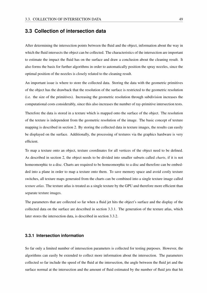
3.3. COLLECTION OF INTERSECTION DATA 49
3.3 Collection of intersection data
After determining the intersection points between the fluid and the object, information about the way in
which the fluid intersects the object can be collected. The characteristics of the intersection are important
to estimate the impact the fluid has on the surface and draw a conclusion about the cleaning result. It
also forms the basis for further algorithms in order to automatically position the spray nozzles, since the
optimal position of the nozzles is closely related to the cleaning result.
An important issue is where to store the collected data. Storing the data with the geometric primitives
of the object has the drawback that the resolution of the surface is restricted to the geometric resolution
(i.e. the size of the primitives). Increasing the geometric resolution through subdivision increases the
computational costs considerably, since this also increases the number of ray-primitive intersection tests.
Therefore the data is stored in a texture which is mapped onto the surface of the object. The resolution
of the texture is independent from the geometric resolution of the image. The basic concept of texture
mapping is described in section 2. By storing the collected data in texture images, the results can easily
be displayed on the surface. Additionally, the processing of textures via the graphics hardware is very
efficient.
To map a texture onto an object, texture coordinates for all vertices of the object need to be defined.
As described in section 2, the object needs to be divided into smaller subsets called charts, if it is not
homeomorphic to a disc. Charts are required to be homeomorphic to a disc and therefore can be embed-
ded into a plane in order to map a texture onto them. To save memory space and avoid costly texture
switches, all texture maps generated from the charts can be combined into a single texture image called
texture atlas. The texture atlas is treated as a single texture by the GPU and therefore more efficient than
separate texture images.
The parameters that are collected so far when a fluid jet hits the object’s surface and the display of the
collected data on the surface are described in section 3.3.1. The generation of the texture atlas, which
later stores the intersection data, is described in section 3.3.2.
3.3.1 Intersection information
So far only a limited number of intersection parameters is collected for testing purposes. However, the
algorithms can easily be extended to collect more information about the intersection. The parameters
collected so far include the speed of the fluid at the intersection, the angle between the fluid jet and the
surface normal at the intersection and the amount of fluid estimated by the number of fluid jets that hit

50 3. REQUIREMENTS AND IMPLEMENTATION
the surface at a certain point. From the latter another parameter can be derived, depicting if the object’s
surface has been reached by the fluid at a certain point or not.
The speed of the fluid at the intersection point is an important parameter to estimate the impact the fluid
has on the surface. Based on the assumption that the fluid propagates with constant speed, the speed v
can be calculated as the norm of the velocity vector ~v.
v = |~v|
However, this only applies to the line representation of the fluid jets, since there is no acceleration. By
taking the acceleration due to gravity g into account, which results in the parabola representation, the
particles no longer move with constant speed. Instead, they are accelerated by gravity. The velocity of
the particles is then defined as the first derivative of the equation of motion (3.2). The speed v of the
particles can again be calculated as the norm of the velocity vector ~v(t).
~v(t) = x(t) = ~vt=0 + 2 · ~g · t
The angle α between the fluid jet and the surface normal ~n also gives information about the fluids impact
on the surface. α can be calculated by applying the following equation, where ~v is the fluid’s velocity
vector.
cos α =−~v · ~n
| − ~v| · |~n|
After calculating the parameter values for a detected intersection point, the data needs to be stored in
the texture. The texture coordinates of the intersection point (i.e. the position in the texture where the
data is stored) can be derived from the texture coordinates of the intersected triangle and the barycentric
coordinates of the intersection point.
~tc(u, v) = (1− u− v) · ~tc0 + u · ~tc1 + v · ~tc2
The barycentric coordinates u and v of the intersection point are determined during the ray - triangle
intersection test as described in section 3.2.1. ~tc0,~tc1 and ~tc2 are the texture coordinates of the triangle
vertices ~v0, ~v1 and ~v2 respectively, determined during the generation of the texture atlas.
Since the texture is a 2D image with discrete pixel coordinates, the texture coordinates of the intersection
point are very unlikely to exactly match a pixel in the image. Therefore each data entry needs to be

3.3. COLLECTION OF INTERSECTION DATA 51
assigned to one discrete value. There are several options for selecting the pixel position. The data entry
is usually assigned to the pixel position that is closest to the texture coordinates of the entry. The value
can be assigned directly to the selected position or the value can be weighted. The weight could be the
distance to the selected pixel. The closer the point is to a pixel, the higher is the percentage of the points
value that is assigned to this pixel.
If more than one data entry in the texture is close to a pixel position, there are several values assigned to
this pixel, each of them associated with a percentage. The final value at the pixel position is determined
by calculating the weighted average x of the assigned values. The percentages associated with the values
xi form the weights ωi.
x =∑n
i=1 ωi · xi∑ni=1 ωi
If the values are assigned without weights, the average can be calculated as follows:
x =∑n
i=1 xi
n
Instead of calculating the average value at a pixel positions, other values such as the sum of all entries at
the pixel could be calculated as well.
After collecting all intersection information and storing the data in texture images, the values can be
transformed into color values, creating false-color images. These images can then be mapped onto
the surface as a texture by the GPU to visualize the collected intersection data directly on the object.
Associating the values with colors enables a faster evaluation of the results.
3.3.2 Texture atlas
The texture atlas, which stores the data collected during the intersection of the fluid with the object, needs
to be generated once for every new object before the object can be sprayed with fluid. The texture coordi-
nates generated by the algorithm described in the following sections are stored in the OBJ file containing
the geometric data of the object and can be reused every time the object is used in the simulation.
The generation of the texture atlas requires two processing steps. First, the object’s surface needs to be
divided into charts. Each chart then has to be unfolded into a plane and parameterized. Second, the
charts need to be packed into one single texture, forming the texture atlas.
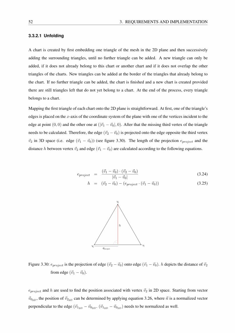
52 3. REQUIREMENTS AND IMPLEMENTATION
3.3.2.1 Unfolding
A chart is created by first embedding one triangle of the mesh in the 2D plane and then successively
adding the surrounding triangles, until no further triangle can be added. A new triangle can only be
added, if it does not already belong to this chart or another chart and if it does not overlap the other
triangles of the charts. New triangles can be added at the border of the triangles that already belong to
the chart. If no further triangle can be added, the chart is finished and a new chart is created provided
there are still triangles left that do not yet belong to a chart. At the end of the process, every triangle
belongs to a chart.
Mapping the first triangle of each chart onto the 2D plane is straightforward. At first, one of the triangle’s
edges is placed on the x-axis of the coordinate system of the plane with one of the vertices incident to the
edge at point (0, 0) and the other one at (|~v1 − ~v0|, 0). After that the missing third vertex of the triangle
needs to be calculated. Therefore, the edge (~v2 − ~v0) is projected onto the edge opposite the third vertex
~v2 in 3D space (i.e. edge (~v1 − ~v0)) (see figure 3.30). The length of the projection eproject and the
distance h between vertex ~v2 and edge (~v1 − ~v0) are calculated according to the following equations.
eproject =(~v1 − ~v0) · (~v2 − ~v0)
|~v1 − ~v0|(3.24)
h = (~v2 − ~v0)− (eproject · (~v1 − ~v0)) (3.25)
!" #!
$!
%&'()*+)
,
Figure 3.30: eproject is the projection of edge (~v2 −~v0) onto edge (~v1 −~v0). h depicts the distance of ~v2
from edge (~v1 − ~v0).
eproject and h are used to find the position associated with vertex ~v2 in 2D space. Starting from vector
~v02D , the position of ~v22D can be determined by applying equation 3.26, where ~n is a normalized vector
perpendicular to the edge (~v12D − ~v02D . (~v12D − ~v02D) needs to be normalized as well.

3.3. COLLECTION OF INTERSECTION DATA 53
~v22D = ~v02D + eproject · (~v12D − ~v02D) + h · ~n (3.26)
After the first triangle has been mapped onto the plane completely, all three half-edges of the triangle are
put in a list for further processing. The list keeps track of all half-edges forming the border of the chart,
where a new triangle could be unfolded. The stack is processed by always taking the first half-edge in
the list and finding the corresponding inverse half-edge. The inverse half-edge is linked to the same edge
but a different triangle (i.e. the triangle on the other side of the edge). The new triangle is tested to see if
it can be added to the chart. If the triangle is added, the list keeping track of the chart border needs to be
updated. Therefore, half-edges that are no longer at the border of the chart are removed and half-edges
from the new triangle, which now are part of the chart border, are added at the end of the list. This way
it is ensured that the chart grows uniformly in all directions around the first triangle. (see figure 3.31)
(a) (b)
(c) (d)
Figure 3.31: Unfolding
To add a new triangle at the current edge, the triangle needs to be mapped onto the plane. Since the 2D
coordinates of one edge already exist, only the 2D coordinates of the vertex opposite this edge have to
be calculated. This is done similarly to calculating the third vertex of the first triangle, which has been
described before by equation 3.26 and is illustrated in figure 3.30. After calculating the coordinates of
the new vertex, the new triangle has to be tested for overlapping with other existing triangles of the chart.
Figure 3.32 shows the general options for two overlapping triangles. However, due to the unfolding

54 3. REQUIREMENTS AND IMPLEMENTATION
(a) (b)
(c) (d)
(e) (f)
Figure 3.32: Triangle overlap: A new triangle that is added to a chart can overlap the other triangles of
the chart, when mapped onto a 2D plane. The new triangle is connected to the chart via one
edge. This leads to the different overlap options displayed in (a) - (d). However, due to the
algorithm applied for unfolding the charts, options (a) and (b) cannot occur here. The only
options for overlap are (c) and (d), where at least one edge of the new triangle crosses one
edge of the border at the chart. (e) and (f) show the valid options for adding the new triangle
to the chart.

3.3. COLLECTION OF INTERSECTION DATA 55
algorithm applied in this case, only options (c) and (d) can occur. In these cases the triangles overlap if
at least two of the triangles’ edges cross. That means, a newly unfolded triangle can only overlap the
chart, if at least one of the triangles edges crosses the border of the chart. Since every new triangle shares
one edge with another triangle of the chart which cannot cross the border of the chart itself, only the
two remaining new edges need to be tested. Border edges which need to be tested for intersection can
be detected via its position relative to the line defined by the edge the chart and the new triangle share.
The chart triangle, which shares this edge always lies on the “inner” side of this line, whereas the new
triangle always lies on the other, the “outer” side of this line, due to the unfolding procedure. Therefore
only border edges with at least one vertex lying on the outer side of the line can be crossed by the new
triangle’s edges. If an efficient classification method exists to find all border edges on the outer side, this
could reduce the amount of overlap tests significantly. However, so far classifying the edges proved more
expensive than simply testing all border edges for overlapping. That is why no procedure to reduce the
number of intersection tests has been applied so far and both edges from the new triangle are tested for
intersection with every single border edge.
!"#"
#$!$
Figure 3.33: The edge defined by vertices ~a1 and ~a2 intersects the edge defined by the vertices~b1 and~b2
To test two edges for intersection, the edges are converted to the following parametric description. ~a1
and ~a2 are the vertices forming the first edge, whereas~b1 and~b2 are the vertices forming the second edge.
(see figure 3.33)
~x(s) = ~a1 + s · (~a2 − ~a1) (3.27)
~x(t) = ~b1 + t · (~b2 −~b1) (3.28)
~x(s) = ~x(t) leads to a system of linear equations, with the following solution for s and t. ~p = (~a2−~a1),
~q = (~b2 −~b1) and ~r = (~b1 − ~a1).
s
−t
=1
~p[0] · ~q[1]− ~p[1] · ~q[0]·
~q [1] −~q [0]
−~p [1] ~p [0]
· ~r (3.29)

56 3. REQUIREMENTS AND IMPLEMENTATION
If both parameters s and t lie between 0 and 1, the edges intersect. This implies that the new triangle
overlaps the chart and therefore cannot be added.
If a triangle that is to be added to the chart shares not only one but two edges with the chart, as is shown
in figure 3.32 (f), one of the edges would generate a positive overlap test, since the edges cross each
other. In this case, the triangle is still added to the chart, since the overlap only occurs due to the fact that
the edges are identical.
Imprecision might occur due to round-off errors of floating point values used for the calculated texture
coordinates as well as the triangles’ positions in 3D space. In this case, triangles which usually should
not overlap cause a positive result in the overlap test. The occurrence of this error can be limited by
tolerating an overlap within a predefined ε region.
3.3.2.2 Packing
After creating all charts, the texture atlas needs to be created by packing the charts into the texture image
defining the atlas. In order to fill the texture atlas efficiently and not waste too much space between the
charts, the charts are ordered according to the size of their bounding box (i.e. the length of the diagonal of
the box) before packing. Additional techniques to adjust the charts exist which might reduce the amount
of texture space wasted even more. One of these more efficient techniques could be implemented in the
future to improve the current algorithm.
After arranging the charts, the skyline algorithm, described in [LPRM02] is applied to pack the charts
into the texture. However, at this stage of development of the CIP simulation, not the actual borders of
the charts are taken into account but the borders of the bounding boxes of the charts, which simplifies the
algorithm. Still, by placing the charts according to their bounding boxes instead of their actual borders,
a certain amount of texture space is wasted. Solving this issue by taking the actual chart borders into
account could by a subject of future work.
Seeing the texture as a (n × n) matrix with n being a power of 2, the skyline in the texture keeps track
of the next free line for each column of the matrix. The skyline is used to find the next valid position
to place the next chart (see figure 3.34). Starting at the lower left corner of the texture, the algorithm
goes through the whole line of the texture to find a location big enough for the chart. The size of the
chart in the texture is determined by a scaling factor, which states the number of pixels assigned per unit
length. If no location is found, the next line above the current line is searched. This step is repeated
until a location is found. After finding the right location for the chart, the skyline is updated with the
upper skyline of the chartÕs box to ensure that the next chart is only placed at a location not occupied

3.3. COLLECTION OF INTERSECTION DATA 57
(a) (b)
Figure 3.34: Packing: A skyline keeps track of the potential positions to pack the charts into the texture
atlas. The skyline is updated by the bounding box of the chart, after it has been packed into
the atlas.
by a previous chart. After packing all charts and assigning new texture coordinates to the half-edges
according to their position in the texture, all texture coordinates need to be scaled down by the size n
of the texture, since the coordinates values are required to be between 0 and 1 to be processed by the
graphics hardware.

58 3. REQUIREMENTS AND IMPLEMENTATION

59
4 Results
As noted in section 1.2, the aim of this project was to create a 3D computer simulation of a CIP system
that could form a basis for testing algorithms in order to automate and optimize the positioning of spray
nozzles in such a system. This chapter presents the functionality of the simulation so far and points out
issues that exist. Additionally, the performance of crucial parts of the simulation is analyzed.
4.1 Functionality
The functionality of the simulation can be divided into three main areas closely related to the three
subtasks that can be derived from the main goal of the project. As mentioned before, these subtasks
include the representation of the CIP system components in 3D space, the simulation of the interaction
between the components as well as the visualization of the characteristics of the interaction.
3D representation The crucial components of a CIP system include the spray nozzles (4.1), the
cleaning fluid (4.2) and the soiled object (4.7). For each component there are several parameters that can
be set by the user. A spray nozzle can be a full cone nozzle (4.3), a hollow cone nozzle (4.4) or a flat fan
nozzle (4.5). A nozzle sprays fluid jets either in the shape of a straight line or in the shape of a parabola.
Interaction between fluid and surface A scene in the CIP system simulation usually consist of
one cleaning object and one or more spray nozzles. (4.8) The fluid jets are tested for intersection with
the object’s surface and jets that touch the surface are reflected. (4.10, 4.11, 4.12) The computation time
for the intersection tests is reduced by using a SAH based kd-tree. (4.9)
Data collection and visualization After the intersection point are determined, several parameter
describing the nature of the interaction (i.e. the speed of the particles, the angle between the fluid jet and
the surface normal and the number of jets per texture element) are calculated, stored in a texture and can
be displayed on the object’s surface.

60 4. RESULTS
(a) (b)
Figure 4.1: (a)A spray nozzle is represented by a cone-shaped primitive and a vector pointing in the
direction the source is aiming at. (b) The parameters of the spray nozzle include parameters
for positioning the nozzle and parameters for adjusting the distribution of the fluid jets.
(a) (b) (c) (d)
Figure 4.2: A fluid jet is represented as either (a) a straight line or (c) a parabola. The number of jets
sprayed from one nozzle can be adjusted by the user. In (b) and (d) the nozzle generates 200
jets.
(a) (b) (c)
Figure 4.3: Full cone nozzle (1000 jets): (a) Sideways view of a full cone nozzle with an aperture angle
of 45◦. (b) Front view of the same nozzle. (c) Full cone nozzle with an aperture angle of 20◦.

4.1. FUNCTIONALITY 61
(a) (b) (c)
Figure 4.4: Hollow cone nozzle (1000 jets): (a) Sideways view of a hollow cone nozzle with an aperture
angle of 45◦ with 90% of the cone being hollow. (b) Front view of the same nozzle. (c)
Hollow cone nozzle with 60% of the cone being hollow.
(a) (b) (c)
Figure 4.5: Flat fan nozzle (1000 jets): (a) Sideways view of a flat fan nozzle with a horizontal aperture
angle of 45◦ and a vertical aperture angle of 20◦. (b) Front view of the same nozzle. (c) Top
view of the nozzle.
(a) (b) (c)
Figure 4.6: Spray patterns: Spray patterns created by (a) a full cone nozzle, (b) a hollow cone nozzle and
(c) a flat fan nozzle.

62 4. RESULTS
(a) (b)
Figure 4.7: (a)The object that is to be cleaned is displayed in a 3D space with a cartesian coordinate
system. The object is represented as a mesh of triangles. (b) There are several parameters
regarding the position and size of the object as well as the display of data on the objects
surface.
(a) (b)
Figure 4.8: Scene: (a) A scene with one object and two spray nozzles, without the fluid jets being dis-
played. (b) The same scene with fluid jets from both scenes reaching the object and being
reflected.

4.1. FUNCTIONALITY 63
(a) (b) (c)
Figure 4.9: Kd-tree: (a) The object is surrounded by an axis-aligned bounding box (red) and the first
split plane is displayed (green) which splits the space of the object into two half spaces. (b)
Both half spaces are split again by individual split planes. (c) The kd-tree is completed as the
termination criterion is met. The bounding boxes of the leaf nodes of the tree are displayed
to mark the leaf nodes (blue).
(a) (b)
Figure 4.10: (a) A straight line that hits the object’s surface is reflected. (b) Several lines that hit the
surface are reflected whereas other lines pass the object.
(a) (b)
Figure 4.11: (a) A parabola that hits the object’s surface is reflected. (b) Several parabolas hitting the
surface are reflected whereas other parabolas pass the object.

64 4. RESULTS
(a) (b) (c)
Figure 4.12: Coefficient of restitution: The reflection angle is determined by the coefficient of restitution
which estimates the influence of the surface material on the reflection. (a) If the coefficient is
0, the reflection angle is equal to the incidence angle and the reflection is a perfect specular
reflection. (b) For a coefficient between 0 and 1, the fluid jet is damped when it hits the
surface. (c) If the coefficient is 1, the jet is damped to an extend that the fluid does not leave
the surface but moves along the surface.
To generate the texture atlas where the intersection data can be stored in, the object needs to be divided
into charts (4.13 and 4.14). The charts are then unfolded and packed into the texture image (4.15).
The visualization of the intersection parameters is effected by different settings. The color scale deter-
mines the color of the texture elements (4.16) and the resolution defines the area of influence of each
fluid jet (4.17). Furthermore, the number of fluid jets generated per nozzle influences the result. (4.18)
The parameters collected at the intersection points include the speed of the particles when hitting the
surface (4.19), the angle between the fluid jets and the surface normal (4.20) and the number of fluid jets
reaching the same element in the texture (4.21). The images show the results of 2000 fluid jets being
sprayed from a full cone spray nozzle with an aperture of 45◦ onto the surface of a cube. The values are
determined by calculating the weighted average and displayed by using different color scales.
4.2 Issues
At the current state of development of the simulation, there are still some issues that need to be corrected
before algorithms for automating the positioning of the spray nozzles can be applied.
The biggest issue forms the storing of intersection data in the texture. So far all charts are packed into
one texture image with the size 1024×1024. While small objects, such as the cube, can easily be packed
into this texture with high resolution, bigger objects, such as the elephant or horse data sets, can only
be packed into the texture with very small resolutions. Due to this, the triangles of the mesh are smaller
than texture elements and more than one triangle lies within one element. When a value is assigned to

4.2. ISSUES 65
(a) (b) (c)
Figure 4.13: Charts: To embed the surface of an object into a plane and map a texture onto it, the surface
needs to be divided into regions homeomorphic to a disc ( = charts). Due to numerical inac-
curacies with floating point values during the generation of the charts, a very high number
of charts is created for complex objects with high curvature.
(a) (b) (c)
Figure 4.14: Charts: The numerical inaccuracies causing a high number of charts to be generated can be
corrected to some extend by allowing the triangles of a chart to overlap within a defined ε
region. This leads to a smaller number of charts, even for complex objects.

66 4. RESULTS
(a) (b)
Figure 4.15: Texture atlas: (a) The surface of the object is divided into charts. (b) The charts are unfolded
and packed into a 2D texture image.
(a) (b) (c) (d)
Figure 4.16: Color scales: The intersection parameters can be displayed on the surface using different
color scales.
(a) (b)
Figure 4.17: Texture resolution: The size of the area in the texture that is effected when a jet hits the
surface can be adjusted by changing the size of the charts in the texture atlas and therefore
the resolution of the texture on the surface.

4.2. ISSUES 67
(a) (b)
Figure 4.18: Number of fluid jets per nozzle: The number of fluid jets sprayed by a nozzle influence how
much of the object’s surface is reached. (a) shows the result of 2000 jets sprayed onto the
surface, while (b) shows the result of 5000 jets.
(a) (b)
Figure 4.19: Particle speed: (a) For the representation of fluid jets as straight lines, the speed of the fluid
particles is constant. (b) For the parabola representation, the fluid particles are accelerated
by gravity and therefore the speed is not constant.

68 4. RESULTS
(a) (b)
Figure 4.20: Intersection angle: (a) The angle between the straight line (i.e. the fluid jet) and the surface
normal is smallest at the center and increases towards the sides. (b) For the parabola repre-
sentation, the smallest angle between the fluid jet and the surface normal is not at the center
but shifted upwards.
(a) (b)
Figure 4.21: Number of jets per texture element: The distribution of the fluid jets is very similar for (a)
straight lines and (b) parabolas. The jets are uniformly distributed throughout the entire
region, with only a slight concentration of jets at the top and bottom.

4.2. ISSUES 69
this texture element, all triangles within this element are displayed in the according color (4.22). This
issue could be solved, by making better use of texture space and using more than one texture image is
the object is too big. However, more texture images also imply more memory space that is required.
(a) (b)
(c) (d)
Figure 4.22: (a) The elephant data set with a small texture resolution is sprayed with fluid jets. (b) Due to
the resolution, other charts that are not hit by the jets but are stored within the same texture
element are falsely marked. (c) If the whole chart is smaller than the texture element, the
whole chart is marked, even though not all parts of the chart are reached by the fluid. (d)
This leads to an area in the shape of the texture being marked instead of the area reached by
the fluid.
Another issues is the number of charts created for the object. A high number of charts means a high
numbers of borders between the charts. These border can cause discontinuity in the display of the
intersection parameters, when a fluid jet hits exactly the border between two charts. Since the charts
are arranged separately in the texture atlas, there is no connectivity information to find the chart next to

70 4. RESULTS
another one.
A further problem is the physical correctness of the fluid representation. Even though the simplified
representations of fluid jets are very efficient for the simulation of the interaction with the object, they
are still only approximations of real spray nozzles. While real fluid jets would interact, creating splashes
that could reach the soiled surface as well, the fluid jets here are independent. This is especially a prob-
lem, when fluid jets from two different nozzles collide. Normally, the fluid jets would be redirected and
splashes would be created. Instead, the fluid jets simply pass each other without interference. Further-
more, part of the real fluid would probably run down the surface after the jets reach the object, cleaning
further parts of the surface to some extend. In the simulation, the fluid jets only influence the part of the
surface that is reached by the jet directly. (4.23)
(a) (b) (c)
Figure 4.23: (a) While usually the surface points that are close to the fluid jets but not hit directly could
be reached by splashing water, the simulation only takes the points into account that are
reached by the jets directly. This can lead to wholes in the spray pattern. (b) Fluid jets from
different spray nozzles pass each other without interference. (c) Fluid running down the
surface after hitting the object are not taken into consideration.
Additionally, there are some problems due to numerical inaccuracies. These problems include the gen-
eration of charts. Furthermore, some intersections between fluid jets and the surface are detected but not
correctly marked in the texture.
Overall, the basic functionality of a CIP system can be illustrated in this simulation. The crucial com-
ponents can be arranged and adjusted in 3D space, though only approximating the real components due

4.3. PERFORMANCE 71
(a) (b)
Figure 4.24: (a) Due to numerical inaccuracies, surfaces that are developable without distortion and
therefore should only create one single chart, are divided into several charts. (b) Some
intersections are not marked in the texture.
to simplifications or computational restrictions. Furthermore, the interaction of the components can be
simulated and the results stored and visualized. However, storing data in a texture and visualizing the
data on the object’s surface only works well for small objects with few charts that can be packed into one
texture image while still enabling a high resolution. For larger objects, the results are not satisfactory
yet, due to the issues mentioned before.
Even though the simulation meets the basic requirements to simulate the functionality of a CIP system,
the prototype is still quite limited regarding the usability and the number of parameters that can be
calculated. This as well as the issues mentioned before leave room for future work in order to achieve
a CIP system simulation that can be used to automate and improve the positioning of spray nozzles in
these systems.
4.3 Performance
In this section the performance of the important algorithms of the simulation is analyzed, by comparing
the amount of time required to apply the algorithm to different data sets. The data sets used are a cube, a
horse and an elephant, which can be seen in the previous section. The following table shows the size of
the triangle meshes representing these objects (see table 4.1).
For the test, two different computers have been used. For the intersection test and the kd-tree construc-
tion, a computer with the following features has been used:
• Intel Pentium 4, 2,6 GHz (2x)

72 4. RESULTS
• 1 GB RAM
• Windows XP (32 Bit)
• GPU: ATI Radeon HD 2600 Pro AGP
For the texture atlas generation test, a computer with the following settings has been used:
• Intel Core 2 Duo, 2,6 GHz
• 4 GB RAM
• Windows Vista (32 Bit)
• GPU: NVIDIA Quadro FX 570M
cube horse elephant
triangles 1.200 39.698 22.840
Table 4.1: Triangles per mesh for the objects used for performance measurements.
The algorithms, whose performances have been tested, include the construction of the kd-tree, the gen-
eration of the texture atlas as well as the interaction of the fluid jets with the triangle mesh. The inter-
section includes finding the intersection points, calculating the intersection parameters and writing the
results into the texture. The tests have been run with different settings to allow for a comparison. The
computation times presented in the following tables are average values.
cube horse elephant
naive kd-tree 0, 199197 2, 03404 1, 38167
SAH kd-tree 0, 13255 4, 69655 2, 759976
Table 4.2: Kd-tree construction: Time (in s) required to build the kd-tree structure for the respective
triangle meshes.
The intersection has been tested by spraying 1000 fluid jets from a full cone spray nozzle onto the triangle
mesh. The test has been done with both straight lines and parabolas in combination with both kd-tree
types. Additionally, the intersection time has been calculated for intersection without a kd-tree (i.e. all
triangles are tested for intersection with every jet). The results are presented in tables 4.3 and 4.4.
As mentioned before, the test for generating the texture atlas and calculating the texture coordinates has
been performed on a different system. (see table 4.5).

4.3. PERFORMANCE 73
cube horse elephant
naive kd-tree 0, 324751 1, 06822 0, 851044
SAH kd-tree 0, 025707 0, 11669 0, 079865
no kd-tree 0, 031059 0, 157991 0, 095248
Table 4.3: Line-object intersection: 1000 straight lines are tested for intersection with the objects.
cube horse elephant
naive kd-tree 0, 251586 1, 54844 0, 952578
SAH kd-tree 0, 088699 0, 276249 0, 194478
no kd-tree 1, 423 26, 5943 22, 5271
Table 4.4: Parabola-object intersection: 1000 parabolas are tested for intersection with the objects.
The results of the performance test reveal the same result that has been mentioned before. It shows
that the generation of the texture atlas is the biggest issue, since it is also the most time consuming
algorithm. The construction of the kd-tree and the intersection of the fluid jets with the object are quite
fast compared to the texture atlas generation. Table 4.2 shows that the construction of the SAH kd tree
is more time consuming than the naive kd-tree, but tables 4.3 and 4.4 show that the SAH kd-tree allows
for a faster intersection of the jets with the object. The results also show that using a kd-tree reduces
the computation time for intersection compared to the time needed for intersection of no kd-tree is used.
Straight line can be processed faster than parabolas for all kd-tree options, which is related to the fact
that the parabola is a quadratic equation whereas the straight line is only a linear equation. Furthermore,
all algorithms scale well for increasing numbers of triangles.

74 4. RESULTS
cube horse elephant
texture atlas 1, 46 193 13, 97
Table 4.5: Texture atlas: average time to calculate the texture coordinates

75
5 Future work
The results presented in chapter 4 point out that the current functionality of the CIP simulation is still very
limited. Therefore, increasing the functionality should be subject to future work. Options for improving
the functionality include collecting more information during the intersection and improving the display
of the results through better color scales. Furthermore, further nozzle types and the combination of
nozzles in clusters could be added. Even rotating nozzles could be studied and added contingent on the
complexity of the task. However, the main functionality that needs to be added is automatic positioning
of spray nozzles. So far, nozzles need to be placed manually.
In addition to expanding the functionality of the simulation, some algorithms currently used could be
improved further. Especially the efficiency of creating the texture atlas could be enhanced. First, instead
of unfolding the charts with a region growing approach, charts could be generated automatically through
more efficient methods such as the least squares conformal maps approach described in [LPRM02]. In
this case the effect of the distortion needs to be considered, though. Second, the skyline algorithm used
to arrange the charts in the atlas could be improved to save texture space by rotating the charts and/or
using the skyline defined by the chart instead of the skyline defined by the chart’s bounding box. (see
figure 5.1)
(a) (b)
Figure 5.1: Charts packed into a texture atlas based on (a) the charts’ exact boundaries or (b) the bounding
box of the charts

76 5. FUTURE WORK
Another algorithm that could be improved is the generation of new jets of fluid from the spray nozzles.
So far a region on the unit sphere around the nozzle is sampled uniformly to generate direction vectors d
for the velocity vectors v of the jets. (see section 3.1) All jets are created with the same speed. However,
the jets are not necessarily all emitted with the same speed from a nozzle. Therefore, generating jets
with varying speed might increase the accuracy of the simulation. The speed values, representing the
pattern created by realistic nozzles, could be stored in a texture mapped onto the unit sphere and sampled
during the generation process. Additionally, the direction vectors d could be generated according to the
distribution in the spray pattern of a nozzle instead of a uniform distribution. The distribution information
from the spray pattern could be stored in the texture with the speed values and sampled during the
generation of the fluid jets. By recording the distribution of the jets and their respective velocities in a
texture and sampling this texture to generate new jets, the simulation would be closer to the real system
and therefore give more accurate results. The feasibility of this approach, however, depends on the
availability of of spray patterns recorded in real CIP systems.
Apart from the algorithms mentioned before, the physical correctness of the simulation leaves room
for further adjustments as well. As there are a number of physical phenomena within a CIP system,
such as the interaction between the fluid jets, which have been disregarded so far, the simulation in
its current state only approximates the functionality of the spray nozzles. Therefore, it is important to
analyze if the implementation is accurate enough to transfer the results to real CIP systems. Maybe a
more exact physically based simulation is necessary to achieve the physical correctness required to make
assumptions that can be transfered to real CIP systems. The drawback of such a simulation, however, is
the complexity and computational intensity of the techniques involved.
In addition to improving existing algorithms and expanding the functionality further, the usability should
be subject to future work as well. Improving the usability could include saving created scenes in a file for
reuse, simplifying the positioning of nozzles via drag&drop and improving the general appearance of the
user interface. Limiting the representation of objects to triangle meshes read from OBJ files also limits
the usability. Therefore, integrating further file formats closer related to CAD systems might increase
the usability for potential users.

77
6 Conclusion
This paper documents the current state of development of the attempt to simulate the functionality of
a CIP system in order to automate the positioning of spray nozzles within the system. The algorithms
applied for achieving the subtasks (i.e representing the components in 3D space, calculating the inter-
action between the components and visualizing the results of the interaction) are explained in detail.
Furthermore, the results at the current state are presented and discussed and existing issues are pointed
out. Finally, options for future work on the simulation are given. Overall, the basic functionality of a
CIP system can be simulated and good results can be achieved especially for smaller objets. Still, the
functionality of the simulation is quite limited due to the time constraints of this project. As described in
section 2 simulating fluids physically correct is a difficult task, due to the number of internal and external
forces that need to be taken into account. Simulating the fluid in close to real time on top of it is almost
impossible, as such a simulation requires a vast amount of computation time. Therefore restrictions need
to be introduced. If, however, a reduced level of precision of the results is acceptable, a simulation of a
CIP system in almost real time with the help of established computer graphics methods is possible. This
forms the basis for applying further algorithms such as next-best-view approaches to automatically plan
the positioning of spray nozzles within the system.

78 6. CONCLUSION

79
Bibliography
[:2006] A guide to safe and efficient tank cleaning. Spraying Systems Co., Catalog 15D,
www.spray.com, 2006.
[App68] Arthur Appel. Some techniques for shading machine renderings of solids. In AFIPS 1968
Spring Joint Computer Conf., volume 32, pages 37–45, 1968.
[BD02] David Benson and Joel Davis. Octree textures. ACM Trans. Graph., 21(3):785–790, 2002.
[BMF07] Robert Bridson and Matthias Müller-Fischer. Fluid simulation: Siggraph 2007 course notes.
In SIGGRAPH ’07: ACM SIGGRAPH 2007 courses, pages 1–81, New York, NY, USA,
2007. ACM.
[CPC84] Robert L. Cook, Thomas Porter, and Loren Carpenter. Distributed ray tracing. SIGGRAPH
Comput. Graph., 18(3):137–145, 1984.
[DDC99] Marlène Dresch, Georges Daufin, and Bernard Chaufer. Membrane processes for the re-
covery of dairy cleaning-in-place solutions. Le Lait, 79(2):245–259, 1999.
[DS03] Carsten Dachsbacher and Marc Stamminger. Translucent shadow maps. In EGRW ’03:
Proceedings of the 14th Eurographics workshop on Rendering, pages 197–201, Aire-la-
Ville, Switzerland, Switzerland, 2003. Eurographics Association.
[DS05] Carsten Dachsbacher and Marc Stamminger. Reflective shadow maps. In I3D ’05: Pro-
ceedings of the 2005 symposium on Interactive 3D graphics and games, pages 203–231,
New York, NY, USA, 2005. ACM.
[ELF05] Douglas Enright, Frank Losasso, and Ronald Fedkiw. A fast and accurate semi-lagrangian
particle level set method. Computers & Structures, 83(6-7):479–490, 2005.
[EMF02] Douglas Enright, Stephen Marschner, and Ronald Fedkiw. Animation and rendering of
complex water surfaces. In SIGGRAPH ’02: Proceedings of the 29th annual conference
on Computer graphics and interactive techniques, pages 736–744, New York, NY, USA,
2002. ACM.

80 Bibliography
[FF01] Nick Foster and Ronald Fedkiw. Practical animation of liquids. In SIGGRAPH ’01: Pro-
ceedings of the 28th annual conference on Computer graphics and interactive techniques,
pages 23–30, New York, NY, USA, 2001. ACM.
[FM96] Nick Foster and Dimitri Metaxas. Realistic animation of liquids. Graphical Models and
Image Processing, 58(5):471–483, 1996.
[GH06] Jostein Gustavsen and Dan Lewi Harkestad. Visualization of water surface using gpu. Mas-
ter’s thesis, Norwegian University of Science and Technology, Department of Computer and
Information Science, 2006.
[Hav00] Vlastimil Havran. Heuristic Ray Shooting Algorithms. PhD thesis, Faculty of Electrical
Engineering, Czech Technical University, Prague, 2000.
[Hav02] Vlastimil Havran. On improving kd-trees for ray shooting. In In Proc. of WSCG 2002
Conference, pages 209–217, 2002.
[HDD+94] Hugues Hoppe, Tony DeRose, Tom Duchamp, Mark Halstead, Hubert Jin, John McDon-
ald, Jean Schweitzer, and Werner Stuetzle. Piecewise smooth surface reconstruction. In
SIGGRAPH ’94: Proceedings of the 21st annual conference on Computer graphics and
interactive techniques, pages 295–302, New York, NY, USA, 1994. ACM.
[HG00] K. Hormann and G. Greiner. MIPS: An efficient global parametrization method. In P.-J.
Laurent, P. Sablonnière, and L. L. Schumaker, editors, Curve and Surface Design: Saint-
Malo 1999, Innovations in Applied Mathematics, pages 153–162. Vanderbilt University
Press, Nashville, TN, 2000.
[HH90] Pat Hanrahan and Paul Haeberli. Direct wysiwyg painting and texturing on 3d shapes.
SIGGRAPH Comput. Graph., 24(4):215–223, 1990.
[IC01] Takeo Igarashi and Dennis Cosgrove. Adaptive unwrapping for interactive texture painting.
In I3D ’01: Proceedings of the 2001 symposium on Interactive 3D graphics, pages 209–
216, New York, NY, USA, 2001. ACM.
[IWP08] Thiago Ize, Ingo Wald, and Steven G. Parker. Ray tracing with the bsp tree. IEEE Sympo-
sium on Interactive Ray Tracing, pages 159 – 166, 2008.
[KCC+06] Janghee Kim, Deukhyun Cha, Byungjoon Chang, Bonki Koo, and Insung Ihm. Practical
animation of turbulent splashing water. In SCA ’06: Proceedings of the 2006 ACM SIG-
GRAPH/Eurographics symposium on Computer animation, pages 335–344, Aire-la-Ville,
Switzerland, Switzerland, 2006. Eurographics Association.

Bibliography 81
[LC87] William E. Lorensen and Harvey E. Cline. Marching cubes: A high resolution 3d surface
construction algorithm. In SIGGRAPH ’87: Proceedings of the 14th annual conference on
Computer graphics and interactive techniques, pages 163–169, New York, NY, USA, 1987.
ACM.
[LM98] Bruno Lévy and Jean-Laurent Mallet. Non-distorted texture mapping for sheared triangu-
lated meshes. In SIGGRAPH ’98: Proceedings of the 25th annual conference on Computer
graphics and interactive techniques, pages 343–352, New York, NY, USA, 1998. ACM.
[LPRM02] Bruno Lévy, Sylvain Petitjean, Nicolas Ray, and Jérome Maillot. Least squares conformal
maps for automatic texture atlas generation. ACM Trans. Graph., 21(3):362–371, 2002.
[Mar03] Steve Marschner. Cs465 notes: Simple ray-triangle intersection.
http://www.cs.cornell.edu/Courses/cs465/2003fa/homeworks/raytri.pdf, October 2003.
[MT97] Tomas Möller and Ben Trumbore. Fast, minimum storage ray-triangle intersection. J.
Graph. Tools, 2(1):21–28, 1997.
[MYV93] Jérôme Maillot, Hussein Yahia, and Anne Verroust. Interactive texture mapping. In SIG-
GRAPH ’93: Proceedings of the 20th annual conference on Computer graphics and inter-
active techniques, pages 27–34, New York, NY, USA, 1993. ACM.
[NH04] Alfred Nischwitz and Peter Haberäcker. Masterkurs Computergrafik und Bildverarbeitung.
Vieweg Verlag, 2004.
[Ped95] Hans Kohling Pedersen. Decorating implicit surfaces. In SIGGRAPH ’95: Proceedings
of the 22nd annual conference on Computer graphics and interactive techniques, pages
291–300, New York, NY, USA, 1995. ACM.
[Pit99] Richard Pito. A solution to the next best view problem for automated surface acquisition.
IEEE Trans. Pattern Anal. Mach. Intell., 21(10):1016–1030, 1999.
[RcUCL03] Nicolas Ray, Jean christophe Ulysse, Xavier Cavin, and Bruno Lévy. Generation of radios-
ity texture atlas for realistic real-time rendering. In Eurographics conf. proc, 2003.
[SB96] Min-Zhi Shao and Norman Badler. Spherical sampling by archimedes’ theorem. Techni-
cal report, Department of Computer and Information Science, University of Pennsylvania,
1996.
[SSGH01] Pedro V. Sander, John Snyder, Steven J. Gortler, and Hugues Hoppe. Texture mapping
progressive meshes. In SIGGRAPH ’01: Proceedings of the 28th annual conference on

82 Bibliography
Computer graphics and interactive techniques, pages 409–416, New York, NY, USA, 2001.
ACM.
[Vic06] Note 5: Cip sytsems. Dairy Food Safety Victoria,
www.dairysafe.vic.gov.au/foodsafetynotes.htm, November 2006.
[Wal04] Ingo Wald. Realtime Ray Tracing and Interactive Global Illumination. PhD thesis, Saarland
University, Saarbrücken, Germany, 2004.
[Wal07] I. Wald. On fast construction of sah-based bounding volume hierarchies. Interactive Ray
Tracing, 2007. RT ’07. IEEE Symposium on, pages 33–40, Sept. 2007.
[WBMS05] Amy Williams, Steve Barrus, R. Keith Morley, and Peter Shirley. An efficient and robust
ray-box intersection algorithm. Journal of Graphics Tools, 10(1):49–54, 2005.
[WBS07] Ingo Wald, Solomon Boulos, and Peter Shirley. Ray tracing deformable scenes using dy-
namic bounding volume hierarchies. ACM Trans. Graph., 26(1):6, 2007.
[WEB08a] Cip cleaning-in-place / sip sterilization-in-place. http://www.niroinc.com/gea_liquid_processing/cleaning_in_place_sip.asp,
October 2008.
[WEB08b] Clean-in-place (cip) applications. http://www.optek.com/Application_Note/General/English/3/Clean-
In-Place_(CIP)_Applications.asp, 10 2008.
[WEB08c] Cleaning in cip processes. http://www.lenntech.com/cleaning-CIP.htm, 10 2008.
[WH06] I. Wald and V. Havran. On building fast kd-trees for ray tracing, and on doing that in o(n
log n). Interactive Ray Tracing 2006, IEEE Symposium on, pages 61–69, Sept. 2006.
[Whi80] Turner Whitted. An improved illumination model for shaded display. Commun. ACM,
23(6):343–349, 1980.
[Won98] Amy C. Lee Wong. Biofilms in food processing environments. Journal of Dairy Science,
81(10):2765–2770, 1998.

83
List of Figures
3.1 Various spray nozzle types [:2006] . . . . . . . . . . . . . . . . . . . . . . . . . . . . . 20
3.2 Generating direction vectors . . . . . . . . . . . . . . . . . . . . . . . . . . . . . . . . 21
3.3 Uniform sampling of sphere . . . . . . . . . . . . . . . . . . . . . . . . . . . . . . . . 22
3.4 Lateral surface of a cylinder . . . . . . . . . . . . . . . . . . . . . . . . . . . . . . . . 22
3.5 Full cone spray nozzle . . . . . . . . . . . . . . . . . . . . . . . . . . . . . . . . . . . 24
3.6 Hollow cone spray nozzle . . . . . . . . . . . . . . . . . . . . . . . . . . . . . . . . . . 24
3.7 Flat fan spray nozzle . . . . . . . . . . . . . . . . . . . . . . . . . . . . . . . . . . . . 25
3.8 Half-edge connectivity . . . . . . . . . . . . . . . . . . . . . . . . . . . . . . . . . . . 27
3.9 Half-edge connectivity 2 . . . . . . . . . . . . . . . . . . . . . . . . . . . . . . . . . . 27
3.10 Half-edge data structure . . . . . . . . . . . . . . . . . . . . . . . . . . . . . . . . . . . 28
3.11 Triangle representation . . . . . . . . . . . . . . . . . . . . . . . . . . . . . . . . . . . 29
3.12 Transformation . . . . . . . . . . . . . . . . . . . . . . . . . . . . . . . . . . . . . . . 30
3.13 Triangle as three overlapping half spaces . . . . . . . . . . . . . . . . . . . . . . . . . . 33
3.14 Barycentric coordinates . . . . . . . . . . . . . . . . . . . . . . . . . . . . . . . . . . . 33
3.15 Kd-tree . . . . . . . . . . . . . . . . . . . . . . . . . . . . . . . . . . . . . . . . . . . 36
3.16 Kd-tree 2 . . . . . . . . . . . . . . . . . . . . . . . . . . . . . . . . . . . . . . . . . . 37
3.17 Split positions . . . . . . . . . . . . . . . . . . . . . . . . . . . . . . . . . . . . . . . . 37
3.18 Surface Area Heursitic . . . . . . . . . . . . . . . . . . . . . . . . . . . . . . . . . . . 39
3.19 Line-box intersection . . . . . . . . . . . . . . . . . . . . . . . . . . . . . . . . . . . . 41
3.20 Line-box intersection 2 . . . . . . . . . . . . . . . . . . . . . . . . . . . . . . . . . . . 41
3.21 Parabola-box intersection . . . . . . . . . . . . . . . . . . . . . . . . . . . . . . . . . . 42
3.22 Parabola-box intersection 2 . . . . . . . . . . . . . . . . . . . . . . . . . . . . . . . . . 42
3.23 Parabola-box intersection 3 . . . . . . . . . . . . . . . . . . . . . . . . . . . . . . . . . 43
3.24 Bounding box . . . . . . . . . . . . . . . . . . . . . . . . . . . . . . . . . . . . . . . . 43
3.25 Parabola-plane intersection . . . . . . . . . . . . . . . . . . . . . . . . . . . . . . . . . 45
3.26 Recursive ray tracing . . . . . . . . . . . . . . . . . . . . . . . . . . . . . . . . . . . . 46
3.27 Law of reflection . . . . . . . . . . . . . . . . . . . . . . . . . . . . . . . . . . . . . . 47

84 List of Figures
3.28 Reflection . . . . . . . . . . . . . . . . . . . . . . . . . . . . . . . . . . . . . . . . . . 47
3.29 Coefficient of restitution . . . . . . . . . . . . . . . . . . . . . . . . . . . . . . . . . . 48
3.30 Unfolding a triangle . . . . . . . . . . . . . . . . . . . . . . . . . . . . . . . . . . . . . 52
3.31 Unfolding a chart . . . . . . . . . . . . . . . . . . . . . . . . . . . . . . . . . . . . . . 53
3.32 Overlapping triangles . . . . . . . . . . . . . . . . . . . . . . . . . . . . . . . . . . . . 54
3.33 Crossing edges . . . . . . . . . . . . . . . . . . . . . . . . . . . . . . . . . . . . . . . 55
3.34 Skyline algorithm for packing charts . . . . . . . . . . . . . . . . . . . . . . . . . . . . 57
4.1 Spray nozzle . . . . . . . . . . . . . . . . . . . . . . . . . . . . . . . . . . . . . . . . . 60
4.2 Fluid . . . . . . . . . . . . . . . . . . . . . . . . . . . . . . . . . . . . . . . . . . . . . 60
4.3 Full cone nozzle . . . . . . . . . . . . . . . . . . . . . . . . . . . . . . . . . . . . . . . 60
4.4 Hollow cone nozzle . . . . . . . . . . . . . . . . . . . . . . . . . . . . . . . . . . . . . 61
4.5 Flat fan nozzle . . . . . . . . . . . . . . . . . . . . . . . . . . . . . . . . . . . . . . . . 61
4.6 Spray patterns . . . . . . . . . . . . . . . . . . . . . . . . . . . . . . . . . . . . . . . . 61
4.7 Object representation . . . . . . . . . . . . . . . . . . . . . . . . . . . . . . . . . . . . 62
4.8 Scene . . . . . . . . . . . . . . . . . . . . . . . . . . . . . . . . . . . . . . . . . . . . 62
4.9 Kd-tree . . . . . . . . . . . . . . . . . . . . . . . . . . . . . . . . . . . . . . . . . . . 63
4.10 Reflected line . . . . . . . . . . . . . . . . . . . . . . . . . . . . . . . . . . . . . . . . 63
4.11 Reflected parabola . . . . . . . . . . . . . . . . . . . . . . . . . . . . . . . . . . . . . 63
4.12 Restitution . . . . . . . . . . . . . . . . . . . . . . . . . . . . . . . . . . . . . . . . . . 64
4.13 Charts . . . . . . . . . . . . . . . . . . . . . . . . . . . . . . . . . . . . . . . . . . . . 65
4.14 Charts 2 . . . . . . . . . . . . . . . . . . . . . . . . . . . . . . . . . . . . . . . . . . . 65
4.15 Texture atlas . . . . . . . . . . . . . . . . . . . . . . . . . . . . . . . . . . . . . . . . . 66
4.16 Color scales . . . . . . . . . . . . . . . . . . . . . . . . . . . . . . . . . . . . . . . . . 66
4.17 Texture resolution . . . . . . . . . . . . . . . . . . . . . . . . . . . . . . . . . . . . . . 66
4.18 Influence of the number of jets per nozzle . . . . . . . . . . . . . . . . . . . . . . . . . 67
4.19 Parameter: particle speed . . . . . . . . . . . . . . . . . . . . . . . . . . . . . . . . . . 67
4.20 Parameter: intersection angle . . . . . . . . . . . . . . . . . . . . . . . . . . . . . . . . 68
4.21 Parameter: number of jets per texel . . . . . . . . . . . . . . . . . . . . . . . . . . . . . 68
4.22 Issues . . . . . . . . . . . . . . . . . . . . . . . . . . . . . . . . . . . . . . . . . . . . 69
4.23 Issues 2 . . . . . . . . . . . . . . . . . . . . . . . . . . . . . . . . . . . . . . . . . . . 70
4.24 Issues 3 . . . . . . . . . . . . . . . . . . . . . . . . . . . . . . . . . . . . . . . . . . . 71
5.1 Skyline algorithm . . . . . . . . . . . . . . . . . . . . . . . . . . . . . . . . . . . . . . 75

85
Acknowledgments
I would like to thank my supervisor Sören König for his constant support, his encouragements and most
of all for his patience.

86 Acknowledgments