Gravitational wave bursts from cosmic (super)strings: Quantitative analysis and constraints

PHYSICAL REVIEW D 73, 105001 (2006)

Gravitational wave bursts from cosmic (super)strings: Quantitative analysis and constraints

Xavier Siemens,1 Jolien Creighton,1 Irit Maor,2 Saikat Ray Majumder,1 Kipp Cannon,1 and Jocelyn Read1

1Center for Gravitation and Cosmology, Department of Physics, University of Wisconsin—Milwaukee, P.O. Box 413,Wisconsin, 53201, USA

2CERCA, Department of Physics, Case Western Reserve University, 10900 Euclid Ave, Cleveland, Ohio 44106-7079 USA(Received 28 February 2006; published 1 May 2006)

1550-7998=20

We discuss data analysis techniques that can be used in the search for gravitational wave bursts fromcosmic strings. When data from multiple interferometers are available, we describe consistency checksthat can be used to greatly reduce the false alarm rates. We construct an expression for the rate of bursts forarbitrary cosmic string loop distributions and apply it to simple known solutions. The cosmology is solvedexactly and includes the effects of a late-time acceleration. We find substantially lower burst rates thanprevious estimates suggest and explain the disagreement. Initial LIGO is unlikely to detect field-theoreticcosmic strings with the usual loop sizes, though it may detect cosmic superstrings as well as cosmicstrings and superstrings with nonstandard loop sizes (which may be more realistic). In the absence of adetection, we show how to set upper limits based on the loudest event. Using Initial LIGO sensitivitycurves, we show that these upper limits may result in interesting constraints on the parameter space oftheories that lead to the production of cosmic strings.

DOI: 10.1103/PhysRevD.73.105001 PACS numbers: 11.27.+d, 11.25.�w, 98.80.Cq

I. INTRODUCTION

Cosmic strings can form during phase transitions in theearly universe [1]. Although cosmic microwave back-ground data has ruled out cosmic strings as the primarysource of density perturbations, they are still potentialcandidates for the generation of a host of interesting as-trophysical phenomena including gravitational waves, ul-tra high energy cosmic rays, and gamma ray bursts. For areview see [2].

Following formation, a string network in an expandinguniverse evolves toward an attractor solution called the‘‘scaling regime’’ (see [2] and references therein). In thisregime, the statistical properties of the system, such as thecorrelation lengths of long strings, scale with the cosmictime, and the energy density of the string network becomesa small constant fraction of the radiation or matter density.

The attractor solution arises due to reconnections, whichfor field-theoretic strings essentially always occur whentwo string segments meet. Reconnections lead to the pro-duction of cosmic string loops, which in turn shrink anddecay by radiating gravitationally. This takes energy out ofthe string network, converting it to gravitational waves. Ifthe density of strings in the network becomes large, thenstrings will meet more often, thereby producing extraloops. The loops then decay gravitationally, removing thesurplus energy from the network. If, on the other hand, thedensity of strings becomes too low, strings will not meetoften enough to produce loops, and their density will startto grow. Thus, the network is driven toward a stableequilibrium.

Recently, it was realized that cosmic strings could beproduced in string-theory inspired inflation scenarios [3–7]. These strings have been dubbed cosmic superstrings.The main differences between field-theoretic strings and

06=73(10)=105001(17) 105001

superstrings are that the latter reconnect when they meetwith probabilities p that can be less than 1, and that morethan one kind of string can form. The values suggested forp are in the range 10�3 � 1 [8]. The suppressed reconnec-tion probabilities arise from two separate effects. The firstis that fundamental strings interact probabilistically, andthe second that strings moving in more than 3 dimensionsmay more readily avoid reconnections: Even though twostrings appear to meet in 3 dimensions, they miss eachother in the extra dimensions [5].

The effect of a small reconnection probability is toincrease the time it takes the network to reach equilibrium,and to increase the density of strings � at equilibrium. Theamount by which the density is increased is the subject ofdebate, with predictions ranging from � / p�2, to � /p�0:6 [6,9,10]. In this work we will assume the densityscales like � / p�1, and that only one kind of cosmicsuperstring is present [11].

Cosmic strings and superstrings can produce powerfulbursts of gravitational waves. These bursts may be detect-able by first generation interferometric earth-based gravi-tational wave detectors such as LIGO and VIRGO [11–13].Thus, the exciting possibility arises that a certain class ofstring theories may have observable consequences in thenear future [14]. It should be noted that if the hierarchyproblem is solved by supersymmetry then the detectabilityof bursts produced by cosmic superstrings is strongly con-strained due to dilaton emission [15].

The bursts we are most likely to be able to detect areproduced at cosmic string cusps. Cusps are regions ofstring that acquire phenomenal Lorentz boosts, withgamma factors �� 1. The combination of the largemass per unit length of cosmic strings and the Lorentzboost results in a powerful burst of gravitational waves.The formation of cusps on cosmic string loops and long

-1 © 2006 The American Physical Society

http://dx.doi.org/10.1103/PhysRevD.73.105001

XAVIER SIEMENS et al. PHYSICAL REVIEW D 73, 105001 (2006)

strings is generic, and their gravitational waveforms aresimple and robust [16].

The three LIGO interferometers (IFOs) are operating atdesign sensitivity. The VIRGO IFO is in the final stages ofcommissioning. Thus, there arises a need for a quantitativeand observationally driven approach to the problem ofbursts from cosmic strings. This paper attempts to providesuch a framework.

We consider the data analysis infrastructure that can beused in the search for gravitational wave bursts fromcosmic string cusps, as well as cosmological burst ratepredictions.

The optimal method to use in the search for signals ofknown form is matched-filtering. In Sec. II we discuss thestatistical properties of the matched-filter output, templatebank construction, an efficient algorithm to compute thematched-filter, and, when data from multiple interferome-ters is available, consistency checks that can be used togreatly reduce the false alarm rate. In Sec. III we discussthe application of the loudest event method to set upperlimits on the rate, the related issue of sensitivity, andbackground estimation. In Sec. IV we derive an expressionfor the rate of bursts for arbitrary cosmic string loopdistributions, and apply it to the distribution proposed inRefs. [11–13]. In Sec. V we compare our estimates for therate with results suggested by previous estimates (in [11–13]). We find substantially substantially lower event rates.The discrepancy arises primarily from our estimate of adetectable burst amplitude, and the use of a cosmology thatincludes the late-time acceleration. We also compute therate for simple loop distributions, using the results ofSec. IVand show how the detectability of bursts is sensitiveto the loop distribution. In Sec. VI we discuss how, in theabsence of a detection, it is possible to use the upper limitson the rate discussed in Sec. III to place interesting con-straints on the parameter space of theories that lead to theproduction of cosmic strings. We show an example of theseconstraints. We summarize our results and conclude inSec. VII.

II. DATA ANALYSIS

A. The signal

In the frequency domain, the waveforms for bursts ofgravitational radiation from cosmic string cusps are givenby [12],

h�f� � Ajfj�4=3��fh � f��f� fl�: (1)

The low frequency cutoff of the gravitational wave signal,fl, is determined by the size of the feature that produces thecusp. Typically this scale is cosmological. In practice,however, the low frequency cutoff of detectable radiationis determined by the low frequency behavior of the instru-ment (for the LIGO instruments, for instance, by seismicnoise). The high frequency cutoff, on the other hand,depends on the angle � between the line of sight and the

105001

direction of the cusp. It is given by,

fh �2

�3L; (2)

where L is the size of the feature that produces the cusp,and in principle can be arbitrarily large. The amplitudeparameter of the cusp waveform A is,

A�G�L2=3

r; (3)

whereG is Newton’s constant,� is the mass per unit lengthof strings, and r is the distance between the cusp andthe point of observation. We have taken the speed of lightc � 1.

The time domain waveform can be computed by takingthe inverse Fourier transform of Eq. (1). The integral has asolution in terms of incomplete Gamma functions. For acusp with peak arrival time at t � 0 it can be written as

h�t� � 2�Ajtj1=3fi��1=3; 2�iflt� � c:c:

� �i��1=3; 2�ifht� � c:c:g: (4)

The duration of the burst is on the order of the inverse ofthe low frequency cutoff fl, and the spike at t � 0 isrounded on a timescale �1=fh.

Equation (4) is useful to make a rough estimate theamplitude of changes in the strain h�t� that a cusp wouldproduce. If we consider a time near t � 0, we can expandthe incomplete Gamma functions according to [17],

��; x� � �� X1n�0

��1�nx��n

n!�� n�: (5)

Keeping the first term of the sum we see that the amplitudein strain of the cusp is,

�hcusp � 6A�f�1=3l � f�1=3

h � 6Af�1=3l ; fh � fl:

(6)

B. Definitions and conventions

The optimal method to use in the search for signals ofknown form is matched-filtering. For our templates we take

t�f� � f�4=3��fh � f��f� fl�; (7)

so that a signal would have h�f� � At�f�. We define theusual detector-noise-weighted inner product [18],

�xjy� � 4<Z 1

0dfx�f�y��f�Sh�f�

; (8)

where Sh�f� is the single-sided spectral density defined byhn�f�n��f0�i � 1

2��f� f0�Sh�f�, where n�f� is the Fourier

transform of the detector noise.The templates of Eq. (7) can be normalized by the inner

product of a template with itself,

-2

GRAVITATIONAL WAVE BURSTS FROM COSMIC . . . PHYSICAL REVIEW D 73, 105001 (2006)

�2 � �tjt� (9)

so that,

t̂ � t=�; and �t̂jt̂� � 1: (10)

If the output of the instrument is s�t�, the signal to noiseratio (SNR) is defined as,

� � �sjt̂�: (11)

In general, the instrument output is a burst h�t� plus somenoise n�t�, s�t� � h�t� � n�t�. When the signal is absent,h�t� � 0, the SNR is Gaussian distributed with zero meanand unit variance,

h�i � h�njt̂�i � 0; h�2i � h�njt̂�2i � 1: (12)

When a signal is present, the average SNR is

h�i � h�hjt̂�i � h�njt̂�i � �A�t̂jt̂� � A�; (13)

and the fluctuations have variance

h�2i � h�i2 � h�h� njt̂�2i � A2�2 � 1: (14)

Thus, when a signal of amplitude A is present, the signal tonoise ratio measured, ~�, is a Gaussian random variable,with mean A� and unit variance,

~� � A� 1 (15)

The amplitude that we assign the event ~A depends on thetemplate normalization �,

~A �~�� A

1

�: (16)

This means that in the presence of Gaussian noise therelative difference between measured and actual signalamplitudes will be proportional to the inverse of the SNR,

�AA�

1

h�i: (17)

If an SNR threshold �th is chosen for the search, on averageonly events with amplitude

Ath ��th

�; (18)

will be detected.

C. Template bank

Cosmic string cusp waveforms have two free parame-ters, the amplitude and the high frequency cutoff. Since theamplitude is an overall scale, the template need not matchthe signal amplitude. However, the high frequency cutoffdoes affect the signal morphology, so a bank of templates isneeded to match possible signals.

The template bank, ftig, where i � 1, 2, . . . N, is one-dimensional, and fully specified by a collection of highfrequency cutoffs ffig. The number of templates N should

105001

be large enough to cover the parameter space finely. Wechoose the ordering of the templates so that fi > fi�1.

Although in principle the high frequency cutoff can beinfinite, in practice the largest distinguishable high fre-quency cutoff is the Nyquist frequency of the time seriescontaining the data, fNyq � 1=�2�t�, where �t is the sam-pling time of that time series. The normalization factor forthe first template is given by

�21 � �t1jt1� � 4<

Z fNyq

fldff�8=3

Sh�f�: (19)

This template is the one with the largest �, and thus thelargest possible SNR at fixed amplitude.

To determine the high frequency cutoffs of the remain-ing templates, we proceed as follows. The fitting factorbetween two adjacent templates ti and ti�1, with highfrequency cutoffs fi and fi�1, is defined as [19]

F ��tijti�1��

�tijti��ti�1jti�1�p � 1� ; (20)

where is the maximum mismatch we choose to allow.The maximum mismatch is twice the maximum fractionalSNR loss due to mismatch between a template in the bankand a signal, and should be small. Since ti�1 has a lowerfrequency cutoff than ti,

�tijti�1� � �ti�1jti�1�: (21)

Thus, the maximum mismatch is,

� 1�

��ti�1jti�1�

�tijti�

s� 1�

�i�1

�i; (22)

and once fixed, determines the high frequency cutoff fi�1,given fi. Thus the template bank can be constructediteratively.

D. Single interferometer data analysis

A convenient way to apply the matched-filter is to usethe inverse spectrum truncation procedure [20]. The usualimplementation of the procedure involves the creation ofan FIR (Finite Impulse Response) digital filter for theinverse of the single-sided power spectral density, Sh�f�,of some segment of data. This filter, along with the tem-plate can then be efficiently applied to the data via FFT(Fast Fourier Transform) convolution. Here we describe avariation of this method in which the template as well asSh�f� are incorporated into the digital filter.

Digital filters may be constructed for each template j inthe bank as follows. First we define a quantity whichcorresponds to the square root of our normalized templatedivided by the single-sided power spectral density,

Tj;1=2�f� �

��t̂j�f�

Sh�f�

s: (23)

-3


This quantity is then inverse Fourier transformed to create,

Tj;1=2�t� �Zdfe2�iftTj;1=2�f�: (24)

At this point the duration of the filter is identical to thelength of data used to estimate the power spectrum Sh�f�.We then truncate the filter, setting to zero values of thefilter sufficiently far from the peak. This is done to limit theamount of data corrupted by filter initialization. Aftertruncation, however, the filter still needs to be sufficientlylong to adequately suppress line noise in the data (such aspower line harmonics). The truncated filter is then forwardFourier transformed, and squared, creating the frequencydomain FIR filter Tj�f�. The SNR is the time series givenby,

�j�t� � 4<Z 1

0dfs�f�Tj�f�e2�ift: (25)

where s�f� is a Fourier transform of the detector straindata.

To generate a discrete set of events or triggers we cantake the SNR time series for each template �j�t� and searchfor clusters of values above some threshold �th. We iden-tify these clusters as triggers and determine the followingproperties: (i) The SNR of the trigger which is the maxi-mum SNR of the cluster; (ii) the amplitude of the trigger,which is the SNR of the trigger divided by the templatenormalization �j; (iii) the peak time of the trigger, which isthe location in time of the maximum SNR; (iv) the starttime of the trigger, which is the time of the first SNR valueabove threshold; (v) the duration of the trigger, whichincludes all values above the threshold; and (vi) the highfrequency cutoff of the template. The final list of triggersfor some segment of data can then be created by choosingthe trigger with the largest SNR when several templatescontain triggers at the same time (within the durations ofthe triggers).

The rate of events we expect can be estimated for thecase of white Gaussian noise. In the absence of a signal theSNR is Gaussian distributed with unit variance. Therefore,at an SNR threshold of �th, the rate of events with � > �th

we expect with a single template is

R�>�th� �t�1Erfc��th=��2p� (26)

where �t is the sampling time of the SNR time series, andErfc is the complementary error function. For example, ifthe time series is sampled at 4096 Hz and an SNR thresholdof 4 is used we expect a false alarm rate of R�>4� 0:26 Hz. The rate of false alarms rises exponentially withlower thresholds.

E. Multiple interferometer consistency checks

When data from multiple interferometers is available, acoincidence scheme can be used to greatly reduce the falsealarm rate of events. For example, in the case of the three

105001

LIGO interferometers, using coincidence would result in acoincident false alarm rate of

R � RH1RH2RL1�2�HH��2�HL�; (27)

where RH1 and RH2 are the rate of false triggers in the 4 kmand 2 km IFOs in Hanford, WA, and RL1 is the rate of falsetriggers in the 4 km IFO in Livingston, LA. The two timewindows �HH, and �HL are the maximum allowed timedifferences between peak times for coincident events in theH1 and H2 IFOs, and H1-L1 (or H2-L1), respectively.Equation (27) follows trivially if the events are Poissondistributed. The factors of 2 multiplying the time windowsarise from the fact that an event in the trigger set of oneinstrument will survive the coincidence if there is an eventin the other instrument within a time � on either side. Thetime windows should allow for light-travel time betweensites, shifting of measured peak location due to noise,timing errors and calibration errors. For example, if wetake �HL � 12 ms and �HH � 2 ms, which allows forthe light-travel time of 10 ms between the Hanford andLivingston sites as well as 2 ms for other uncertainties, andthe single IFO false alarm rate estimated in the previoussubsection (0.26 Hz), we obtain a triple coincident falsealarm rate,

R 1:7� 10�6 Hz; (28)

which is about 50 false events per year.Additionally, when two instruments are coaligned, such

as the H1 and H2 LIGO IFOs, we can demand some degreeof consistency in the amplitudes recovered from thematched-filter (see, for example, the distance cut used in[21]). If the instruments are not coaligned then the ampli-tudes recovered by the matched-filter could be different.This is due to the fact that the antenna pattern of theinstrument depends on the source location in the sky. Ifthe event is due to a fluctuation of the noise or an instru-mental glitch we do not generally expect the amplitudes intwo coaligned IFOs to agree. The effect of Gaussian noiseto 1 � on the estimate of the amplitude can be read fromEq. (17). This equation can be used to construct an ampli-tude veto. For example, to veto events in H1 we candemand

AH1 � AH2

AH1<

��H1� �

�; (29)

where � is the number of standard deviations we allow and� is an additional fractional difference in the amplitude thataccounts for other sources of uncertainty (such as thecalibration).

These tests can be used to construct the final trigger set,a list of survivors for each of our instruments which havepassed all the consistency checks.

-4


III. UPPER LIMITS, SENSITIVITY ANDBACKGROUND

In this section we describe the application of the loudestevent method [22] to our problem, address the related issueof sensitivity, and discuss background estimation.

We define the loudest event to be the survivor with thelargest amplitude. Suppose, in one of the instruments, wefind the loudest event to have an amplitude A�. For anobservation time T, on average, the number of events weexpect to show up with an amplitude greater than A� is

N>A� � T�; (30)

where the effective rate is defined as

� �Z 1

0�A�; A�

dR�A�dA

dA: (31)

Here, �A�; A� is the search efficiency, namely, the fractionof events with an optimally oriented amplitude A found atthe end of the pipeline with an amplitude greater than A�.Aside from sky location effects, the measured amplitude ofevents is changed as a result of the noise (see Eq. (17)). Theefficiency can be measured by adding simulated signals todetector noise, and then searching for them. The efficiencyaccounts for the properties of the population, such as thedistribution of sources in the sky and the different highfrequency cutoffs (as we will see, dR=df / f�5=3 forcusps), as well as possible inefficiencies of the pipeline.The quantity

dR�A�dA

dA (32)

is the cosmological rate of events with optimally orientedamplitudes between A and A� dA and will be the subjectof the next section.

If the population produces Poisson distributed events,the probability that no events show up with a measuredamplitude greater than A�, in an observation time T, is

P � e�T�: (33)

The probability, �, that at least one event with amplitudegreater than A� shows up is � � 1� P, so that if � � 0:9,90% of the time we would have expected to see an eventwith amplitude greater than A�.

From Eq. (33) we see that,

ln�1� �� T�; (34)

Setting � � 0:9, say, we have

�90% 2:303

T: (35)

We say that the value of � < �90% with 90% confidence, inthe sense that if � � �90%, 90% of the time we would haveobserved at least one event with amplitude greater than A�.If we take a nominal observation time of 1 yr, T � 3:2�107 s, our upper limit statement becomes,

105001

� < �90% 2:303=year 7:3� 10�8 s�1: (36)

This bound on the effective rate can be used to constrainthe parameters of cosmic string models that enter throughthe cosmological rate dR=dA in Eq. (31).

The efficiency �A�; A� is the fraction of events withoptimally oriented amplitude A which show up in our finaltrigger set with an amplitude greater than A�. If A� A�

then we expect �A�; A� 1, and when A� A�,�A�; A� 0. If A50% is the amplitude at which half ofthe signals are found with an amplitude greater than A�, wecan approximate the sigmoid we expect for the efficiencycurve by,

�A�; A� ��A� A50%�; (37)

meaning we assume all events in the data with an ampli-tude A > A50% survive the pipeline and are found with anamplitude greater than A�. This means we can approximatethe rate integral � of Eq. (31) as,

� Z 1A50%

dR�A�dA

dA � R>A50%; (38)

so that if R>A50%>�90% for a particular model of cosmic

strings, the model can be excluded (in the frequentistsense) at the 90% level. We expect A50% to be proportionalto A�. It is at least a factor of

��5p

larger, due to the averagingof source locations on the sky [23], and potentially evenlarger than this due inefficiencies of the data analysispipeline. If there are no significant inefficiencies then weexpect A50%

��5pA�.

At design sensitivity the form of the Initial LIGO noisecurve may be approximated by [24],

Sh�f� ��

1:09� 10�41

�30 Hz

f

�28

� 1:44� 10�45

�100 Hz

f

�4

� 1:28� 10�46

�1�

�f

90 Hz

�2��

s: (39)

The first term is the so-called seismic wall, the second termcomes from thermal noise in the suspension of the optics,and the third term from photon shot noise. In the absence ofa signal, this curve can be used to estimate the amplitude oftypical noise induced events.

As pointed out in [11], a reasonable operating point forthe pipeline involves an SNR threshold of �th � 4. Thevalue of the amplitude is related to �, the SNR, and �, thetemplate normalization,

�2 � 4<Z 1

0df

t�f�2

Sh�f�� 4

Z fh

fldff�8=3

Sh�f�(40)

by Eq. (18). If the loudest surviving event has an SNR closeto the threshold, �� 4, a low frequency cutoff at fl �40 Hz (the seismic wall is such that it is not worth running

-5


the matched-filter below 40 Hz), and a typical high fre-quency cutoff fh � 150 Hz then the amplitude of theloudest event will be A� 4� 10�21 s�1=3. So we expectA50% 9� 10�21 s�1=3 for the Initial LIGO noise curve.

The question of the sensitivity of the search is subtlydifferent. In this case we are interested in how many burstevents we can detect at all, not just those with amplitudesgreater than A�. The rate of events we expect to be able todetect is thus,

�s �Z 1

0�0; A�

dR�A�dA

dA: (41)

The efficiency includes events of all amplitudes and if thecosmological rate dR=dA favors low amplitude events, thisrate could be larger than that given by Eq. (30). Fur-thermore this rate should be compared with a rate of1=T, rather than, say, the 90% rate of Eq. (35). The neteffect is that the parameter space of detectability can besubstantially larger than the parameter space over whichwe can set upper limits. It should be noted that the 0 in thefraction of detected events �0; A� in Eq. (41) means thatwe only demand that events with optimally oriented am-plitudes A show up in the final trigger (not that theiramplitudes be larger than A�). There is in fact a minimumdetectable amplitude of events, given by Amin � �th=�max,where �max is the largest template normalization used inthe search.

In the remainder of the paper we will use an amplitudeestimate of A50% � 10�20 s�1=3 for Initial LIGO upperlimit and sensitivity estimates. Advanced LIGO is ex-pected to be somewhat more than an order of magnitudemore sensitive then Initial LIGO, so for the AdvancedLIGO rate estimates we will use A50% � 10�21 s�1=3. Itshould be noted that the loudest event resulting from asearch on IFO data could be larger than this, for instance ifit was due to a real event or a surviving instrumental glitch.

The rate of events that we expect in the absence of asignal, called the background, can be estimated eitheranalytically (via Eq. (27), in which the single IFO ratesare measured), or by performing time-slides (see, for ex-ample [25]). In the latter procedure single IFO triggers aretime-shifted relative to each other and the rate of accidentalcoincidences is measured. Care must be taken to ensure thetime-shifts are longer than the duration of real events. If therate of events is unknown, then one can look for statisti-cally significant excesses in the foreground data set. In thiscase a statistically significant excess could point to adetection. However, as we shall see, there is enough free-dom in models of string evolution to lead to statisticallyinsignificant excesses in any background. Therefore it isprudent to carefully examine the largest amplitude surviv-ing triggers regardless of consistency with the background.

105001

IV. THE RATE OF BURSTS

In this section we will derive the expression for thecosmological rate as a function of the amplitude, whichis needed to evaluate the upper limit and sensitivity inte-grals (Eqs. (30) and (41)). To make this account self-contained we will rederive a number of the results pre-sented in [11–13]. The main differences from the previousapproach are that we derive an expression for a generalcosmic string loop distribution that can be used when sucha distribution becomes known, we absorb some uncertain-ties of the model, as well as factors of order 1, into a set ofignorance constants, and we consider a generic cosmologywith a view to including the effects of a late-timeacceleration.

Numerical simulations show that at any cosmic time t,the network consists of a few long strings that stretchacross the horizon and a large collection of small loops.In early simulations [26] the size of loops, as well as thesubstructure on the long strings, was at the size of thesimulation resolution. At the time of the early simulations,the consensus reached was that the size of loops andsubstructure on the long strings was at the size given bygravitational back-reaction. Very recent simulations [27–29] suggest that the size of loops is given by the large scaledynamics of the network, and is thus unrelated to thegravitational back-reaction scale. Further work is neces-sary to establish which of the two possibilities is correct.

In either case, the size of loops can be characterized by aprobability distribution,

n�l; t�dl; (42)

the number density of loops with sizes between l and l�dl at a cosmic time t. This distribution is unknown, thoughanalytic solutions can be found in simple cases (see [2]Sec. 9.3.3).

The period of oscillation of a loop of length l is T � l=2.If, on average, loops have c cusps per oscillation, thenumber of cusps produced per unit space-time volume byloops with lengths in the interval dl at time t is [30]

�l; t�dl �2cln�l; t�dl: (43)

We can write the cosmic time as a function of the redshift,

t � H�10 ’t�z�; (44)

where H0 is current value of the Hubble parameter and’t�z� is a function of the redshift z which depends on thecosmology. In [11–13], an approximate interpolating func-tion for ’t�z� was used for a universe which containsmatter and radiation. For the moment we will leave itunspecified. Later we will compute it numerically for amore realistic cosmology which includes the late-timeacceleration. We can therefore write the number of cuspsper unit space-time volume produced by loops with sizes

-6


between l and l� dl at a redshift z,

�l; z�dl �2cln�l; z�dl: (45)

Now we would like to write the length of loops in termsof the amplitude of the event an optimally oriented cuspfrom such a loop would produce at an earth-based detector.The amplitude we expect from a cusp produced at a red-shift z, from a loop of length l can be read off Eq. (4.10) of[13]. It is

A � g1G�l2=3H0

�1� z�1=3’r�z�: (46)

Here g1 is an ignorance constant that absorbs the uncer-tainty on exactly how much of the length l is involved inthe production of the cusp, as well as factors of O�1� thathave been dropped from the calculation (see the derivationleading up to Eq. (3.12) in [13]). If loops are not too wiggly,we expect this ignorance constant to be of O�1�. We haveexpressed r�z�, the amplitude distance [13], as an unspeci-fied cosmology dependent function of the redshift ’r�z�,

r�z� � H�10 ’r�z�: (47)

The amplitude distance is a factor of �1� z� smaller thanthe luminosity distance. Since,

l�A; z� ��A’r�z��1� z�1=3

g1G�H0

�3=2; and

dldA�

3

2Al;

(48)

we can write the number of cusps per unit space-timevolume which produce events with amplitudes between Aand A� dA from a redshift z as,

�A; z�dA �3cAn�l�A; z�; z�dA: (49)

As discussed in [12], we can observe only a fraction ofall the cusps that occur in a Hubble volume. Suppose welook, via matched-filtering, for signals of the form ofEq. (1). The highest frequency we observe fh is relatedto the angle � that the line of sight makes to the direction ofthe cusp. If f� is the lowest high frequency cutoff that ourinstrument can detect with confidence, the maximum anglethe line of sight and the direction of a detectable cusp cansubtend is,

�m � �g2f�l��1=3: (50)

The ignorance constant g2 absorbs a factor of about 2.31[13], other factors of O�1�, as well as the fraction of theloop length l that actually contributes to the cusp (see thederivation leading up to Eq. (3.22) of [13]). Just like for ourfirst ignorance constant g1, if loops are not too wiggly, weexpect g2 to be of O�1�. For bursts originating at cosmo-logical distances, red-shifting of the high frequency cutoff

105001

must be taken into account. So we write,

�m�z; f�; l� � �g2�1� z�f�l�1=3; (51)

The waveform in Eq. (1), was derived in the limit ��1, so that cusps with � * 1 will not have the form of Eq. (1)(indeed, they are not bursts at all). Therefore cusps with� * 1 should not contribute to the rate. Thus, the fractionof cusps that are observable, �, is

��z; f�; l� �2m�z; f�; l�

4��1� �m�z; f�; l��: (52)

The first term on the right hand side is the beaming fractionfor the angle �m. At fixed l, the beaming fraction is thefraction of cusp events with high frequency cutoffs greaterthan f�. The � function cuts off cusp events that have�m � 1; it ensures we only count cusps whose waveform isindeed given by Eq. (1).

The rate of cusp events we expect to see from a volumedV�z� (the proper volume in the redshift interval dz), in anamplitude interval dA is [31]

dRdV�z�dA

� �1� z��1 �A; z��z; f�; A�; (53)

where ��z; f�; A� � ��z; f�; l�A; z��. The factor of �1�z��1 comes from the relation between the observed burstrate and the cosmic time: Bursts coming from large red-shifts are spaced further apart in time. We write the propervolume element as,

dV�z� � H�30 ’V�z�dz; (54)

where ’V�z� is a cosmology dependent function of theredshift. Thus, for arbitrary loop distributions, we can writethe rate of events in the amplitude interval dA, needed toevaluate the upper limit integral Eq. (30), and sensitivityintegral Eq. (41) as,

dRdA� H�3

0

Z 10dz’V�z��1� z��1 �A; z��z; f�; A�:

(55)

Damour and Vilenkin [11–13] took the loop distributionto be

n�l; t� � �p�G��1t�3��l� �t�; (56)

where p is the reconnection probability, which can besmaller than 1 for cosmic superstrings. The constant � isthe ratio of the power radiated into gravitational waves byloops to G�2, and thus related to the lifetime of loops. It ismeasured in numerical simulations to be �� 50.

In this loop distribution all loops present at a cosmictime t, are of the same size �t. The distribution is consis-tent with the assumption usually made in the literature thatthe size of loops is given by gravitational back-reaction,and that �� G�. Recently it was realized that dampingof perturbations propagating on strings due to gravitationalwave emission is not as efficient as previously thought

-7


[32]. As a consequence, the size of the small-scale struc-ture is sensitive to the spectrum of perturbations present onthe strings, and can be much smaller than the canonicalvalue �G�t [33].

If the value of � is given by gravitational back-reactionwe can write it as

� � "��G��n: (57)

We use two parameters ", introduced in [11], as well as nthat can be used to vary the size of loops. The parameter narises naturally from gravitational back-reaction modelsand is related to the power spectrum of perturbations onlong strings [33]. For example, if the spectrum is inverselyproportional to the mode number, then n � 3=2. This is thespectrum of perturbations we expect if, say, the shape ofthe string is dominated by the largest kink [33].

As we have mentioned, recent simulations suggest thatloops are produced at sizes unrelated to the gravitationalback-reaction scale [27–29]. If this is the case, then theloops produced survive for a long time, and the form of thedistribution can be computed analytically in the matter andradiation eras using some simple assumptions (see [2]Sec. 9.3.3).

In general the rate integral needs to be computed, pre-sumably numerically, through Eq. (55). In the case of themore simple loop distribution of Eq. (56), it is convenientto proceed slightly differently. In this case all loops at agiven redshift are of the same size, so we can directlyassociate amplitudes with redshifts.

We can write the rate of cusp events we expect to seefrom the redshift interval dz, from loops of length in theinterval dl as

dRdzdl

� H�30 ’V�z��1� z�

�1 �l; z��z; f�; l�: (58)

Using Eq. (45) and (56) with t expressed in terms of theredshift, and integrating over l we find,

dRdz� H0

c�g2f�H�10 �

�2=3

2�5=3p�G�’�14=3t �z�’V�z��1� z�

�5=3

��1� �m�z; f�; �H�10 ’t�z�� (59)

At a redshift of z, all cusps produce bursts of the sameamplitude, given by replacing l with �H�1

0 ’t�z� inEq. (46). Therefore the solution of,

’2=3t �z�

�1� z�1=3’r�z��

AH�1=30

g1G��2=3

(60)

for z gives the redshift from which a burst of amplitude Aoriginates. This means we can perform the rate integral,say Eq. (38), over redshifts rather than over amplitudes,

� Z z50%

0

dRdzdz; (61)

where z50% is the solution of Eq. (60) for A � A50%.

105001

To compute the cosmological functions, ’t�z�, ’r�z�,and ’V�z�, we use the set of cosmological parameters in[34], which provide a good fit to recent cosmological data.The precise values of the parameters are not critical, butwe include them here for clarity. They are, H0 �73 km s�1 Mpc�1 � 2:4� 10�18 s�1, �m � 0:25, �r �4:6� 10�5, and �� 1��m ��r. The derivation ofthe three cosmological functions is included inAppendix A for completeness and result in the cosmologi-cal functions Eqs. (A4), (A6), and (A8). In the remainder ofthe paper we will refer to this cosmological model as the �universe.

V. RESULTS I: DETECTABILITY

A. Comparison with previous estimates

In [11–13] Damour and Vilenkin considered a universewith matter and radiation. They introduced a set of ap-proximate interpolating functions for ’t�z�, ’r�z�, and’V�z�. They were

’t�z� � t0H0�1� z��3=2�1� z=zeq�

�1=2; (62)

’r�z� � t0H0z

1� z; (63)

and [35],

’V�z� � �t0H0�3102z2�1� z��13=2�1� z=zeq�

�1=2: (64)

Damour and Vilenkin used zeq 103:9 as the redshift ofradiation matter equality and set the age of the universet0 � 1017:5 s. Notice that if we substitute Eqs. (62) and(64) into Eq. (59) and set � � �G� and g2 � p � 1 werecover Eq. (5.17) of [13] (aside from a factor of z relatedto their use of a logarithmic derivative).

We will use Eqs. (62)–(64) to compare the previousresults [11–13] with those of a cosmology solved exactlyincluding the effects of a late-time acceleration, i.e. thecosmological functions Eqs. (A4), (A6), and (A8). Damourand Vilenkin considered the amplitude (in strain) of eventsat a fixed rate of 1 per year and compared that to an SNR 1,optimally oriented event (see, for example, the dashedhorizontal lines of Fig. 1 in [13]). Instead, we have startedby estimating a detectable signal amplitude, and computedthe event rate at and above that amplitude.

Bursts from cosmic string cusps are Poisson distributed.The quantity we have computed, �, is the rate of events inour data set with amplitudes greater than A50%. In anobservation time T the probability of not having such anevent is exp��T�. Hence, the odds of having at least leastone event in our data set with amplitude larger than ourminimum detectable amplitude is,

� � 1� e��T: (65)

Figure 1 shows the rate of burst events, �, as well as theprobability � of having at least least one event in our data

-8

10−12

10−11

10−10

10−9

10−8

10−7

10−6

10−5

10−4

10−18

10−16

10−14

10−12

10−10

10−8

10−6

Gµ

γ [H

z]

10−12

10−11

10−10

10−9

10−8

10−7

10−6

10−5

10−4

10−10

10−8

10−6

10−4

10−2

100

Gµ

η

Λ Cosmology A50%

=10−20 s−1/3

Λ Cosmology A50%

=10−21 s−1/3

DV Cosmology A50%

=10−20 s−1/3

DV Cosmology A50%

=10−21 s−1/3

Λ Cosmology A50%

=10−20 s−1/3

Λ Cosmology A50%

=10−21 s−1/3

DV Cosmology A50%

=10−20 s−1/3

DV Cosmology A50%

=10−21 s−1/3

1/year

FIG. 1. Plot of the rate of gravitational wave bursts, � (toppanel), and the probability � of having at least least one event inour data set with amplitude larger than A50% in a year ofobservation (bottom panel), as a function of G�. For all curveswe have set � � �G�, � � 50, f� � 75 Hz, c � p � 1, andthe ignorance constants g1 � g2 � 1. The dash-dot and dashedcurves show � and � computed with the Damour-Vilenkincosmological functions Eqs. (62)–(64), with A50% �10�21 s�1=3, and A50% � 10�20 s�1=3 respectively. The thickand thin solid curves show � and � computed in a universewith a cosmological constant with amplitudes A50% �10�20 s�1=3, and A50% � 10�21 s�1=3 respectively.


set with amplitude larger than A50% for a year of observa-tion, as a function of G� for two different models. For allcurves we have set � � �G�, � � 50, f� � 75 Hz, c �p � 1, and the ignorance constants g1 � g2 � 1. We willrefer to string models with these parameters as ‘‘classic’’,which is appropriate for field-theoretic strings with loopsof size l � �G�t. The dashed-dot and dashed curves ofFig. 1 show � and � computed using the Damour-Vilenkincosmological functions, namely, Eqs. (62)–(64). For thedashed-dot curves we have used an amplitude estimate ofA50% � 10�21 s�1=3. This amplitude estimate can be ob-tained using the Initial LIGO sensitivity curve, setting theSNR threshold to 1, and assuming all cusp events areoptimally oriented (as used for the dashed horizontal linesof Fig. 1 in [13]). This is also our estimate for the ampli-tude in the case of Advanced LIGO. The dashed curvesshow � and � computed with the amplitude A50% �

10�20 s�1=3, which we feel is more appropriate for InitialLIGO. The thick and thin solid curves show � and �computed by evaluating the cosmological functions

105001

(Eqs. (A4), (A6), and (A8)) numerically for the � universe(see Appendix A). The thick solid curves correspond to ouramplitude estimate for Initial LIGO, and the thin solidcurves to our estimate for Advanced LIGO.

The functional dependence of the rate of gravitationalwave bursts on G� is discussed in detail in Appendix B.Here we summarize those findings. From left to right, thefirst steep rise in the rates as a function ofG� of the dashedand dashed-dot curves of Fig. 1 comes from events pro-duced at small redshifts (z� 1). The peak and subsequentdecrease in the rate starting around G�� 10�9 comesfrom events produced at larger redshifts but still in thematter era (1� z� zeq). The final rise comes from eventsproduced in the radiation era (z� zeq).

For classic cosmic strings (p � " � n � 1), the matter-era maximum in our estimate for the rate of events at InitialLIGO sensitivity is about 7� 10�4 events per year, whichis substantially lower than the rate �1 per year suggestedby the results of Damour and Vilenkin [11–13]. The bulk ofthe difference arises from our estimate of a detectableamplitude. This is illustrated by the dashed-dot and dashedcurves of Fig. 1, which use the same cosmological func-tions, and two estimates for the amplitude, A50% �

10�21 s�1=3 and A50% � 10�20 s�1=3 respectively. Our am-plitude estimate results in a decrease in the burst rate byabout a factor of 100 at the matter-era peak. A moredetailed discussion of the effect of the amplitude on therate can be found in Appendix B. The remaining discrep-ancy arises from differences in the cosmology, as well asfactors ofO�1� that were dropped in the previous estimates,which account for a further decrease by factor of about10. This is illustrated by the difference between the dashed-dot and thin solid curves of Fig. 1, which use the sameamplitude estimate A50% � 10�21 s�1=3, and the Damour-Vilenkin cosmological interpolating functions (Eqs. (62)–(64)) and the � universe functions (Eqs. (A4), (A6), and(A8)), respectively. When z� 1, the effects of a cosmo-logical constant are unimportant and differences arise fromfactors ofO�1� that were dropped in the previous estimates.For z * 1, the differences arise from a combination of theeffects of a cosmological constant as well as factors ofO�1�. The net effect is that the chances of seeing an eventfrom classic strings using Initial LIGO data have droppedfrom order unity to about 10�3 at the matter-era peak.This is illustrated by the difference between the dashed-dot and thick solid curves of Fig. 1. The dashed-dot curveswere computed using the amplitude estimate A50% �

10�21 s�1=3 and the Damour-Vilenkin interpolating cos-mological functions, whereas the thick solid curves use anamplitude estimate of A50% � 10�20 s�1=3 in the �universe.

Cosmic superstrings, however, may still be detectable byInitial LIGO. Furthermore, if the size of the small-scalestructure is given by gravitational back-reaction, reason-able estimates for what the size of loops might be also lead

-9

10−12

10−11

10−10

10−9

10−8

10−7

10−6

10−5

10−4

10−20

10−15

10−10

10−5

100

Gµ

γ [H

z]

10−8

10−6

10−4

10−2

100

η

Λ Cosmology A50%

=10−21 s−1/3, p=10−3

Λ Cosmology A50%

=10−21 s−1/3, n=3/2Λ Cosmology A =10−21 s−1/3, n=3/2, p=10−3

Λ Cosmology A50%

=10−21 s−1/3, p=10−3

Λ Cosmology A50%

=10−21 s−1/3, n=3/2Λ Cosmology A

50%=10−21 s−1/3, n=3/2, p=10−3

1/year


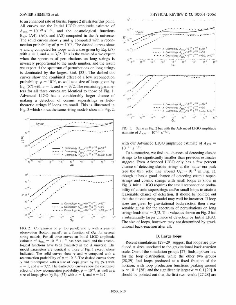
to an enhanced rate of bursts. Figure 2 illustrates this point.All curves use the Initial LIGO amplitude estimate ofA50% � 10�20 s�1=3, and the cosmological functionsEqs. (A4), (A6), and (A8) computed in the � universe.The solid curves show � and � computed with a recon-nection probability of p � 10�3. The dashed curves show� and � computed for loops with a size given by Eq. (57)with " � 1, and n � 3=2. This is the value of n we expectwhen the spectrum of perturbations on long strings isinversely proportional to the mode number, and the resultwe expect if the spectrum of perturbations on long stringsis dominated by the largest kink [33]. The dashed-dotcurves show the combined effect of a low reconnectionprobability, p � 10�3, as well as a size of loops given byEq. (57) with " � 1, and n � 3=2. The remaining parame-ters for all three curves are identical to those of Fig. 1.Advanced LIGO has a considerably larger chance ofmaking a detection of cosmic superstrings or field-theoretic strings if loops are small. This is illustrated inFig. 3 which shows the same string models shown in Fig. 2,

10−12

10−11

10−10

10−9

10−8

10−7

10−6

10−5

10−4

10−10

Gµ

50%

FIG. 3. Same as Fig. 2 but with the Advanced LIGO amplitudeestimate of A50% � 10�21 s�1=3.

10−12

10−11

10−10

10−9

10−8

10−7

10−6

10−5

10−4

10−20

10−15

10−10

10−5

Gµ

γ [H

z]

10−12

10−11

10−10

10−9

10−8

10−7

10−6

10−5

10−4

10−12

10−10

10−8

10−6

10−4

10−2

100

Gµ

η

Λ Cosmology A50%

=10−20 s−1/3, p=10−3

Λ Cosmology A50%


50%=10−20 s−1/3, n=3/2, p=10−3

Λ Cosmology A50%

=10−20 s−1/3, p=10−3

Λ Cosmology A50%


50%=10−20 s−1/3, n=3/2, p=10−3

1/year

FIG. 2. Comparison of � (top panel) and � with a year ofobservation (bottom panel), as a function of G� for severalstring models. For all three curves an Initial LIGO amplitudeestimate of A50% � 10�20 s�1=3 has been used, and the cosmo-logical functions have been evaluated in the � universe. Themodel parameters are identical to those of Fig. 1 except whereindicated. The solid curves show � and � computed with areconnection probability of p � 10�3. The dashed curves show� and � computed with a size of loops given by Eq. (57) with" � 1, and n � 3=2. The dashed-dot curves show the combinedeffect of a low reconnection probability, p � 10�3, as well as asize of loops given by Eq. (57) with " � 1, and n � 3=2.

105001

with our Advanced LIGO amplitude estimate of A50% �

10�21 s�1=3.To summarize, we find the chances of detecting classic

strings to be significantly smaller than previous estimatessuggest. Even Advanced LIGO only has a few percentchance of detecting classic strings at the matter-era peak(see the thin solid line around G�� 10�9 in Fig. 1),though it has a good chance of detecting cosmic super-strings and cosmic strings with small loops as show inFig. 3. Initial LIGO requires the small reconnection proba-bility of cosmic superstrings and/or small loops to attain areasonable chance of detection. It should be pointed outthat the classic string model may well be incorrect. If loopsizes are given by gravitational backreaction then a rea-sonable guess for the spectrum of perturbations on longstrings leads to n � 3=2. This value, as shown on Fig. 2 hasa substantially larger chance of detection by Initial LIGO.The size of loops, however, may not determined by gravi-tational back-reaction after all.

B. Large loops

Recent simulations [27–29] suggest that loops are pro-duced at sizes unrelated to the gravitational back-reactionscale. One of the simulation groups [27] finds a power lawfor the loop distribution, while the other two groups[28,29] find loops produced at a fixed fraction of thehorizon, with loop production functions peaking around� 10�3 [28], and the significantly larger � 0:1 [29]. Itshould be pointed out that the first two results [27,28] are

-10

10−12

10−11

10−10

10−9

10−8

10−7

10−6

10−5

10−4

10−18

10−16

10−14

10−12

10−10

10−8

10−6

Gµ

γ [H

z]

10−12

10−11

10−10

10−9

10−8

10−7

10−6

10−5

10−4

10−10

10−8

10−6

10−4

10−2

100

Gµ

η

Eq. (56)Eqs. (68)−(70), α=0.1Eq. (71), β=5/2, B=0.15

Eq. (56)Eqs. (68)−(70), α=0.1Eq. (71), β=5/2, B=0.15

1/year

FIG. 4. Plot of the rate of bursts � (top panel), and �, theprobability of having at least one event in our data set withamplitude larger than A50% in a year of observation (bottompanel), as a function of G� for various loops distributions. Forall curves we have set � � 50, f� � 75 Hz, c � p � 1, and theignorance constants g1 � g2 � 1. As a reference we again show� and � computed using the loop distribution from Eq. (56),according to Eq. (59), in the �-universe with � � �G� usingthe solid curve. The remaining curves have been computedthrough Eqs. (38) and (55) with A50% � 10�20 s�1=3. The dashedcurves show � and � computed using the loop distribution ofEqs. (68)–(70). The dashed-dot curves show � and � computedwith Eq. (71).


expanding universe simulations, whereas the results of thethird group [29] come from simulations in Minkowskispace.

Following formation, the length of loops shrinks due togravitational wave emission according to [2],

l�t� � li � �G��t� ti�; (66)

where li � �ti, is the initial length, and ti is the time offormation of the loop. The length goes to zero at time

tf ��

�G�� 1

�ti: (67)

Loops are long-lived when tf � ti, i.e. when �=��G�� 1. For � 0:1, using � � 50 the lifetime of loops is longprovided G�� 2� 10�3, which covers the entire rangeof astrophysically interesting values of G�. On the otherhand, if we take � 5� 10�4, then loops are long-livedonly when G�� 10�5.

If the size of loops is given by gravitational backreac-tion, then � is given by Eq. (57), and provided n � 1 allloops are short-lived. This means we can use n�l; t� /��l� �t� (as we have so far) because the loop distributionis dominated by the loops that just formed.

If loops are long-lived, the distribution can be calculatedif a scaling process is assumed (see [2], Secs. 9.3.3 and10.1.2). In the radiation era it is

n�l; t� � �rt�3=2�l� �G�t��5=2; l < �t; t < teq

(68)

where �r 0:4��1=2, and � is a parameter related to thecorrelation length of the network found in numerical simu-lations of radiation era evolution to be about 15 (seeTable 10.1 in [2]). The upper bound on the length arisesbecause no loops are formed with sizes larger than �t.

In the matter era the distribution has two components,loops formed in the matter era and survivors from theradiation era. Loops formed in the matter era have lengthsdistributed according to,

n1�l; t� � �mt�2�l� �G�t��2;

�teq � �G��t� teq�< l < �t; t > teq

(69)

with �m 0:12� , with � 4 (see Table 10.1 in [2]). Thelower bound on the length is due to the fact that thesmallest loops present in the matter era started with alength �teq when they were formed and their lengthshave since decreased due to gravitational wave emission.Additionally there are loops formed in the radiation erathat survive into the matter era. Their lengths are distrib-uted according to,

n2�l; t� � �rt1=2eq t�2�l� �G�t��5=2;

l < �teq � �G��t� teq�; t > teq;(70)

where the upper bound on the length comes from the factthat the largest loops formed in the radiation era had a size

105001

�teq but have since shrunk due to gravitational waveemission.

The simulations in [27] find a power law for the loopdistribution, n�l� / l��. If all loops produced are long-lived, meaning no loops are produced with sizes below�G�t, the distribution we expect is

n�l; t� � Bt��4�l� �G�t��: (71)

The most recent fits to their loop distribution find� 5=2,in both the radiation and matter eras, and B 0:1, 0.2 inthe matter and radiation eras respectively [36].

We can use the results of Sec. IV to compute the rate ofbursts for these loop distributions. Figure 4 shows the burstrate �, and the probability � of having at least least oneevent in our data set with amplitude larger than A50% in ayear of observation as a function of G� for all the abovedistributions. For all curves we have set � � 50, f� �75 Hz, c � p � 1, and the ignorance constants g1 � g2 �1. We have evaluated the cosmological functions in the �

-11

10−12

10−11

10−10

10−9

10−8

10−7

10−6

10−5

10−4

10−15

10−10

10−5

Gµ

γ [H

z]

10−12

10−11

10−10

10−9

10−8

10−7

10−6

10−5

10−4

10−8

10−6

10−4

10−2

100

Gµ

η

Eq. (56)Eqs. (68)−(70), α=0.1Eq. (71), β=5/2, B=0.15

Eq. (56)Eqs. (68)−(70), α=0.1Eq. (71), β=5/2, B=0.15

1/year

FIG. 5. Same as Fig. 4 but using our Advanced LIGO ampli-tude estimate A50% � 10�21 s�1=3.


universe. As a reference, we again show � and � computedusing the loop distribution from Eq. (56), according toEq. (59), with � � �G� using the solid curves. Theremaining curves have been computed through Eqs. (38)and (55) with A50% � 10�20 s�1=3. The dashed curvesshow � and � computed using the loop distribution ofEqs. (68)–(70) with � � 0:1. The dashed-dot curvesshow � and � computed with Eq. (71), where we havetaken� � 5=2, and B � 0:15 as an approximation for boththe radiation and matter eras. Figure 5 shows the same loopdistributions as Fig. 4 but using our Advanced LIGOamplitude estimate A50% � 10�21 s�1=3.

The loop distributions shown here lead to a significantenhancement in the rate. Note that we have not includedthe enhancement in the rate of bursts for the case of cosmicsuperstrings p < 1. Given the range of results, it is impor-tant to determine whether the loop sizes at formation aredetermined by gravitational back-reaction, or whether theyare large and we require a revised loop distribution.

VI. RESULTS II: CONSTRAINTS

If no events can be positively identified in a search, wecan use the results of Sec. III to constrain the parameterspace of theories that lead to the production of cosmicstrings. Unfortunately, as we have mentioned, considerableuncertainties remain in models of cosmic string evolution.Nevertheless, we can place constraints that are correct inthe context of a particular string model. Here we will

105001

illustrate the procedure for the loop distribution, Eq. (56),and the resulting rate Eq. (59).

We would like to absorb the ignorance constants g1 andg2 into the parameters of the model. The two ignoranceconstants enter the expression for the rate Eq. (59) in threeways. First, they affect the upper limit of the integralEq. (61) through Eq. (60), which is,

’2=3t �z�

�1� z�1=3’r�z��

AH�1=30

g1G��2=3: (72)

Secondly, they enter through �m in the theta-function cut-off of the rate,

�m � �g2�1� z�f��H�10 ’t�z��1=3; (73)

and finally, the rate itself (Eq. (59)) is proportional tog�2=3

2 .If we write � � "��G��n, and substitute into Eqs. (72)

and (73), we can simultaneously absorb g1 and g2 into newvariables ~"�"; g1; g2; n� and X�G�; g1; g2�. Looking atEq. (73) we can write an identity for the ignorance con-stants and the variables we want to absorb them into,

g2"��G��n � ~"��X�n: (74)

Similarly, looking at the denominator of the right hand sideof Eq. (72) we write,

g1G��"��G��n2=3 � X�~"��X�n2=3 (75)

These equations can be simultaneously solved to give,

G� � g�11 g2=3

2 X; (76)

and

" � gn1g�2n=3�12 ~": (77)

If we replace G� by Eq. (76) and " by Eq. (77), in Eq. (73)we obtain,

�m � ��1� z�f�~"��X�nH�1

0 ’t�z��1=3; (78)

and if we make the same replacements into Eq. (72),

’2=3t �z�

�1� z�1=3’r�z��

AH�1=30

X�~"��X�n�2=3; (79)

namely, we obtain functions of ~" and X only.Finally, if we replace G� by Eq. (76) and " by Eq. (77),

in our expression for the rate, Eq. (59), we see that we canabsorb the remaining factors by defining a quantity,

� � g1=32 g1

cp: (80)

This yields a rate,

dRdz� H0

��f�H�10 �

�2=3

2�~"��X�n�5=3�X’�14=3t �z�’V�z��1� z�

�5=3

��1� �m�; (81)

-12

g−11

g−1/32

p/c (=1/β) 6

8%

95%

99.

7%

g 1 g−

2/3

2 G

µ (

=X

)

10−5

10−4

10−3

10−2

10−1

100

10−10

10−9

10−8

10−7

10−6

Allowed Region

Region ruled outat the 99.7% level

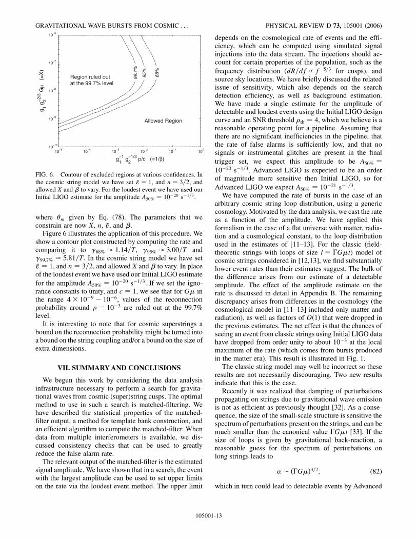
FIG. 6. Contour of excluded regions at various confidences. Inthe cosmic string model we have set ~" � 1, and n � 3=2, andallowed X and � to vary. For the loudest event we have used ourInitial LIGO estimate for the amplitude A50% � 10�20 s�1=3.


where �m given by Eq. (78). The parameters that weconstrain are now X, n, ~", and �.

Figure 6 illustrates the application of this procedure. Weshow a contour plot constructed by computing the rate andcomparing it to �68% 1:14=T, �95% 3:00=T and�99:7% 5:81=T. In the cosmic string model we have set~" � 1, and n � 3=2, and allowed X and � to vary. In placeof the loudest event we have used our Initial LIGO estimatefor the amplitude A50% � 10�20 s�1=3. If we set the igno-rance constants to unity, and c � 1, we see that for G� inthe range 4� 10�9 � 10�6, values of the reconnectionprobability around p � 10�3 are ruled out at the 99.7%level.

It is interesting to note that for cosmic superstrings abound on the reconnection probability might be turned intoa bound on the string coupling and/or a bound on the size ofextra dimensions.

VII. SUMMARY AND CONCLUSIONS

We begun this work by considering the data analysisinfrastructure necessary to perform a search for gravita-tional waves from cosmic (super)string cusps. The optimalmethod to use in such a search is matched-filtering. Wehave described the statistical properties of the matched-filter output, a method for template bank construction, andan efficient algorithm to compute the matched-filter. Whendata from multiple interferometers is available, we dis-cussed consistency checks that can be used to greatlyreduce the false alarm rate.

The relevant output of the matched-filter is the estimatedsignal amplitude. We have shown that in a search, the eventwith the largest amplitude can be used to set upper limitson the rate via the loudest event method. The upper limit

105001

depends on the cosmological rate of events and the effi-ciency, which can be computed using simulated signalinjections into the data stream. The injections should ac-count for certain properties of the population, such as thefrequency distribution (dR=df / f�5=3 for cusps), andsource sky locations. We have briefly discussed the relatedissue of sensitivity, which also depends on the searchdetection efficiency, as well as background estimation.We have made a single estimate for the amplitude ofdetectable and loudest events using the Initial LIGO designcurve and an SNR threshold �th � 4, which we believe is areasonable operating point for a pipeline. Assuming thatthere are no significant inefficiencies in the pipeline, thatthe rate of false alarms is sufficiently low, and that nosignals or instrumental glitches are present in the finaltrigger set, we expect this amplitude to be A50% �

10�20 s�1=3. Advanced LIGO is expected to be an orderof magnitude more sensitive then Initial LIGO, so forAdvanced LIGO we expect A50% � 10�21 s�1=3.

We have computed the rate of bursts in the case of anarbitrary cosmic string loop distribution, using a genericcosmology. Motivated by the data analysis, we cast the rateas a function of the amplitude. We have applied thisformalism in the case of a flat universe with matter, radia-tion and a cosmological constant, to the loop distributionused in the estimates of [11–13]. For the classic (field-theoretic strings with loops of size l � �G�t) model ofcosmic strings considered in [12,13], we find substantiallylower event rates than their estimates suggest. The bulk ofthe difference arises from our estimate of a detectableamplitude. The effect of the amplitude estimate on therate is discussed in detail in Appendix B. The remainingdiscrepancy arises from differences in the cosmology (thecosmological model in [11–13] included only matter andradiation), as well as factors of O�1� that were dropped inthe previous estimates. The net effect is that the chances ofseeing an event from classic strings using Initial LIGO datahave dropped from order unity to about 10�3 at the localmaximum of the rate (which comes from bursts producedin the matter era). This result is illustrated in Fig. 1.

The classic string model may well be incorrect so theseresults are not necessarily discouraging. Two new resultsindicate that this is the case.

Recently it was realized that damping of perturbationspropagating on strings due to gravitational wave emissionis not as efficient as previously thought [32]. As a conse-quence, the size of the small-scale structure is sensitive thespectrum of perturbations present on the strings, and can bemuch smaller than the canonical value �G�t [33]. If thesize of loops is given by gravitational back-reaction, areasonable guess for the spectrum of perturbations onlong strings leads to

�� G��3=2; (82)

which in turn could lead to detectable events by Advanced

-13


LIGO, or Initial LIGO if we are dealing with cosmicsuperstrings. This is illustrated in Figs. 2 and 3.

Even more recently, simulations [27–29] suggest thatloops are produced at sizes unrelated to the gravitationalback-reaction scale, � & 1. In this case loops of manydifferent sizes are present at any given time (becausethey are very long-lived), and the use of a revised loopdistribution becomes necessary. The particulars of thedistribution are currently under debate, but all distributionscurrently considered lead to an enhanced rate of burstsrelative to the classic model. Results for the rate for variousloop distributions are shown in Figs. 4 and 5.

Finally, we have shown how the parameter space oftheories that lead to the production of cosmic strings mightbe constrained in the absence of a detection. Results for amodel of cosmic superstrings, where the loop size is givenby Eq. (82), are shown in Fig. 6. Initial LIGO may yieldinteresting constraints on the reconnection probability forsome range of string tensions. Intriguingly, a bound on thereconnection probability might be turned into a bound onthe string coupling and/or a bound on the size of extradimensions, in the case of cosmic superstrings.

Wish list

Unfortunately, there remain considerable uncertaintiesin models of cosmic string evolution. While we can esti-mate the detectability, and place constraints, that are cor-rect in the context of a particular string model, the currentparameter space allows for a wide spectrum of burst ratesin the interesting range of string tensions.

We would like to finish by posing a set of questions tothe various cosmic string simulation groups which, fromthe perspective of gravitational wave detection, wouldgreatly improve predictability.

They are:
(i) W hat is the size of cosmic string loops? Are they
large when they are formed, so we need to considera loop distribution? If so, what is that distribution?Is their size instead given by gravitational back-reaction? If so, what is the spectrum of perturba-tions on long strings?

(ii) W
hat is the number of cusps per loop oscillation? Isit independent of the loop size?
(iii) W
hat is the size of cusps? In particular, what frac-tion of the loop length l is involved in the cusp?
(iv) W
hat are the effects of low reconnection probabil-ity? In particular, what is the enhancement in theloop density that results?
ACKNOWLEDGMENTS

We are especially grateful to Alex Vilenkin and KenOlum for carefully reading the paper and suggesting sev-eral important improvements and corrections. We are alsograteful to Vicky Kalogera, Richard O’Shaughnessy andThibault Damour for carefully reading the paper and pro-

105001

viding many helpful suggestions and improvements.Finally, we would like to thank Benjamin Wandelt andMarialessandra Papa for useful discussions, ChrisRingeval for useful and friendly correspondence, andDaniel Sigg for providing the analytic form for the LIGOdesign curve, Eq. (39). The work of X. S., J. C., S. R. M.,J. R., and K. C. was supported by NSF grant Nos. PHY0200852 and PHY 0421416. The work of I. M. was sup-ported by the DOE and NASA.

APPENDIX A: COSMOLOGICAL FUNCTIONS

To derive exact expressions for ’t�z�, ’r�z�, and ’V�z�,we begin with the evolution of the Hubble function. TheHubble function is given by

H�z� � H0h�z�; (A1)

with, for a flat universe,

h�z� � ��m�1� z�3 ��r�1� z�4 ��1=2: (A2)

Here, �i � �i�z � 0�=�c�z � 0� is the present energydensity of the i’th component, relative to the critical den-sity. The subscripts m, r, and � stand for matter (dark andbaryonic), radiation, and the cosmological constant, re-spectively. Since we assume the universe flat, ��i � 1.

We will use the set of cosmological parameters in [34],which provide a good fit to recent cosmological data. Theprecise values of the parameters are not critical, but weinclude them here for clarity. They are, H0 �73 km s�1 Mpc�1 � 2:4� 10�18 s�1, �m � 0:25, �r �4:6� 10�5, and �� 1��m ��r.

To compute the relation between the time and the red-shift, we use the fact that dz=dt � ��1� z�H, and write

t �Z t

0dt0 �

Z 1z

dz0

�1� z0�H�z0�: (A3)

The dimensionless function ’t�z� of Eq. (44) is thus,

’t�z� �Z 1z

dz0

�1� z0�h�z0�: (A4)

In order to compute the amplitude distance [13] as afunction of the redshift, we consider null geodesics in anFRW universe. We can take the polar and azimuthal coor-dinates to be constant and let the radial coordinate, r, vary.In this case we have that dr=dt � ��1� z�, and thusdr=dz � 1=H. So we write

r �Z r

0dr0 �

Z z

0

dz0

H�z0�: (A5)

We can therefore express the dimensionless function ofEq. (47), ’r�z�, as

’r�z� �Z z

0

dz0

h�z0�: (A6)

-14


Finally, we would like to derive an expression for thedifferential volume as a function of the redshift, dV=dz.The differential volume element is given by

dV � a3�t�r2dr sin�d�d�;

where a�t� is the scale factor. Integrating over the polar andazimuthal coordinates and using dr=dz gives

dV � 4�a3�t�r2dr �4�r2

�1� z�3H�z�dz: (A7)

Using Eqs. (A1) and (A5) gives the dimensionless functionof Eq. (54)

’V�z� �4�’2

r�z�

�1� z�3h�z�: (A8)

APPENDIX B: APPROXIMATE ANALYTICEXPRESSION FOR THE RATE

In this appendix we compute an approximate expressionfor the rate as a function of the amplitude can be obtainedusing the interpolating functions introduced in [11–13],Eqs. (62)–(64). The result is useful to understand thequalitative behavior of the rate curves shown in Figs. 1–3.

Using Eqs. (46) and (63) we can write the amplitude ofan burst from a loop of length l at a redshift z as

A�G�l2=3�1� z�2=3

t0z: (B1)

We take the size of the feature that produces the cusp to bethe typical size of loops, l�z� � �H�1

0 ’t�z�, with ’t�z�given by Eq. (62), so that,

A�G��2=3t�1=30 z�1�1� z��1=3�1� z=zeq�

�1=3: (B2)

We define a dimensionless amplitude a,

a �A

G��2=3t�1=30

� z�1�1� z��1=3�1� z=zeq��1=3

(B3)

Depending on the value of z, the function a�z� has threedifferent asymptotic behaviours,

a�z� �

8><>:z�1 z� 1z�4=3 1� z� zeq

z1=3eq z�5=3 z� zeq

(B4)

The regime where z� 1 corresponds to cusp events oc-curring nearby, the regime where 1� z� zeq corre-sponds to matter-era events, and the regime wherez� zeq corresponds to radiation era events.

At z � 1, we define

a1 � a�z � 1� 2�1=3 � 1;

and at z � zeq,

105001

aeq � a�z � zeq� z�4=3eq 2�1=3 z�4=3

eq a1 4� 10�6:

This means we can write,

zeq � a�3=4eq : (B5)

The regime where z� 1, corresponds to a� 1; theregime where 1� z� zeq, corresponds to aeq � a� 1;and the regime where z� zeq, corresponds to a� aeq.This means that we can write,

z�a� �

8><>:a�3=20

eq a�3=5 a� aeq

a�3=4 aeq � a� 1a�1 a� 1

(B6)

We can write this in terms of the interpolating function,

z�a� � a�3=20eq a�3=5

�1�

aaeq

��3=20

�1� a��1=4: (B7)

Using Eqs. (62) and (64), we can write the rate of eventsas a function of the redshift, Eq. (59), as,

dRdz� bz2�1� z��7=6�1� z=zeq�

11=6; (B8)

where b is defined as

b � 102c��5=3�p�G��1t�10 �f�t0�

�2=3; (B9)

and the theta-function cutoff has been ignored for conve-nience. In the three regimes considered above the rate isgiven by,

dR� b�

8><>:z2dz z� 1z5=6dz 1� z� zeq

z�11=6eq z8=3dz z� zeq

(B10)

In the regime where z� 1, corresponds to a� 1, andz� a�1. This means,

dR� bz2dz � ba�2 dzdada: (B11)

Since,

dzda��a�2; (B12)

we have that

dR��ba�4da; for a� 1: (B13)

The regime where 1� z� zeq, corresponds to aeq �

a� 1, and z� a�3=4. This means,

dR� bz5=6dz � ba�5=8 dzdada: (B14)

Since,

dzda��

3

4a�7=4; (B15)

-15


we have that

dR��3

4ba�19=8da; for aeq � a� 1: (B16)

Finally, the regime where z� zeq, corresponds to a�aeq, and z� �aeq=a1�

�3=20a�3=5. Thus, using Eq. (B5),

dR� bz�11=6eq z8=3dz � ba39=40

eq a�8=5 dzdada: (B17)

Since,

dzda��

3

5a�3=20

eq a�8=5; (B18)

we have that

dR��3

5ba33=40

eq a�16=5da; for a� aeq: (B19)

Summarising,

dR�a�da

��b�

8><>:a33=40

eq a�16=5 a� aeq

a�19=8 aeq � a� 1a�4 a� 1

(B20)

Equation (B20) can be integrated, to give the rate of eventswith reduced amplitude greater than a,

R>a � b�

8><>:a33=40

eq a�11=5 a� aeq

a�11=8 aeq � a� 1a�3 a� 1

(B21)

We can determine the functional dependence of the ratefor the simple case when � � �G�, which we can thencompare with the dashed and dashed-dot curves of Fig. 1.The factor of b, as defined by Eq. (B9), contains a factor of�G��1 as well as a factor of �G��5=3 through its depen-dence on �. So we take b / �G��8=3. The dimensionlessamplitude a, as defined by Eq. (B3) also contains a factorof �G��1 as well as a factor of �G��2=3 through itsdependence on �, so that a / �G��5=3.

In Eq. (B21), (as we have mentioned) the regime wherea� aeq maps into the radiation era, and in this case therate,

105001

R / G�: (B22)

The regime where aeq � a� 1 maps into the matter erawhen the redshift z� 1, and the rate in this case is,

R / �G��31=24: (B23)

The final regime when a� 1 corresponds to bursts that arecoming from close by (z� 1), and the rate,

R / �G��7=3: (B24)

So we immediately see that the first steep rise in the rate asa function of G� (from left to right) of the dashed anddashed-dot curves of Fig. 1 corresponds to bursts that arecoming from small redshifts, i.e. from z� 1. The slightdecrease in the rate comes from bursts produced at largeredshifts, but still in the matter era, i.e. 1� z� zeq, andthe final increase in the rate comes from bursts produced inthe radiation era, z� zeq.

Equation (B21) also makes it easy to understand thelower burst event rates we find relative to the previousestimates of Damour and Vilenkin [11–13] (see the dashedand dashed-dot curves of Fig. 1). They compared the strainproduced by cosmic string burst events at a rate of 1 peryear to a noise induced SNR 1 event, given the Initial LIGOdesign noise curve (see, for example, the dashed lines inFig. 1 of [11]). In our treatment, the amplitude that corre-sponds to is A � 10�21 s�1=3. To make our amplitudeestimate we have chosen an SNR threshold of 4, which,as proposed in [11], is a reasonable operating point for adata analysis pipeline, and have included the effects of theantenna pattern of the instrument, which averages to afactor of

��5p

. The combined effect is to increase the am-plitude estimate by about a factor of 10, to make it A 10�20 s�1=3.

Looking at Eq. (B21), we see that an increase in theamplitude of a factor of 10, results in a decrease of a factorof 103 in the rate of nearby bursts (z� 1), a decrease by afactor of about 24 in the rate of bursts produced in thematter era (1� z� zeq), and a decrease by about a factorof 160 in the rate of bursts produced in the radiation era(z� zeq).

[1] T. W. B. Kibble, J. Phys. A 9, 1387 (1976).[2] A. Vilenkin and E. P. S. Shellard, Cosmic Strings and

Other Topological Defects (Cambridge University Press,Cambridge, 2000).

[3] N. Jones, H. Stoica, and S. H. Henry Tye, J. High EnergyPhys. 07 (2002) 051.

[4] S. Sarangi and S. H. Henry Tye, Phys. Lett. B 536, 185(2002).

[5] G. Dvali and A. Vilenkin, J. Cosmol. Astropart. Phys. 03(2004) 010.

[6] N. Jones, H. Stoica, and S. H. Henry Tye, Phys. Lett. B563, 6 (2003).

[7] E. J. Copeland, R. C. Myers, and J. Polchinski, J. HighEnergy Phys. 06 (2004) 013.

[8] M. G. Jackson, N. T. Jones, and J. Polchinski, J. HighEnergy Phys. 10 (2005) 013.

-16


[9] M. Sakellariadou, J. Cosmol. Astropart. Phys. 04 (2005)003.

[10] A. Avgoustidis and E. P. S. Shellard, astro-ph/0512582.[11] T. Damour and A. Vilenkin, Phys. Rev. D 71, 063510

(2005).[12] T. Damour and A. Vilenkin, Phys. Rev. Lett. 85, 3761

(2000).[13] T. Damour and A. Vilenkin, Phys. Rev. D 64, 064008

(2001).[14] J. Polchinski, hep-th/0410082; hep-th/0412244.[15] E. Babichev and M. Kachelriess, Phys. Lett. B 614, 1

(2005).[16] X. Siemens and K. D. Olum, Phys. Rev. D 68, 085017

(2003).[17] I. S. Gradstheyn and I. M. Ryzhyk, Table of Integrals

Series and Products (unpublished).[18] C. Cutler and E. E. Flanagan, Phys. Rev. D 49, 2658

(1994).[19] B. J. Owen, Phys. Rev. D 53, 6749 (1996).[20] B. Allen, W. G. Anderson, P. R. Brady, D. A. Brown, and

J. D. E. Creighton, gr-qc/0509116.[21] B. Abbott et al. (LIGO Scientific Collaboration), Phys.

Rev. D 72, 082001 (2005).[22] P. R. Brady, J. D. E. Creighton, and A. G. Wiseman, Class.

Quant. Grav. 21, S1775 (2004).[23] K. S. Thorne, 300 Years of Gravitation (Cambridge

University Press, Cambridge, 1987).[24] A. Lazzarini and R. Weiss, LIGO technical report, LIGO

Report No. LIGO-E950018-02, 1996; A. Abramoviciet al., Science 256, 325 (1992); Thorne, Drever, Weiss,

105001

and Raab, National Science Foundation ProposalNo. PHY-9210038, 1989.

[25] B. Abbott et al. (LIGO Scientific Collaboration), Phys.Rev. D 69, 102001 (2004).

[26] A. Albrecht and N. Turok, Phys. Rev. D 40, 973 (1989);D. P. Bennett and F. R. Bouchet, Phys. Rev. D 41, 2408(1990); B. Allen and E. P. S. Shellard, Phys. Rev. Lett. 64,119 (1990).

[27] C. Ringeval, M. Sakellaridou, and F. Bouchet, astro-ph/0511646.

[28] C. J. A. P. Martins and E. P. S. Shellard, Phys. Rev. D 73,043515 (2006).

[29] V. Vanchurin, K. D. Olum, and A. Vilenkin, gr-qc/0511159.

[30] Here we have assumed that the number of cusps peroscillation does not depend on the length of the loop.This will be true provided that loops have the same shape(statistically), regardless of their size.

[31] In [11–13], the cutoff was placed on the strain of cusps (ata fixed rate) rather than their rate, as we do here. This isunimportant, the purpose of the theta function is to ensurewe do not overestimate the rate.

[32] X. Siemens and K. D. Olum, Nucl. Phys. B611, 125(2001).

[33] X. Siemens, K. D. Olum, and A. Vilenkin, Phys. Rev. D66, 043501 (2002).

[34] S. Eidelman et al., Phys. Lett. B 592, 1 (2004); A. R.Liddle and O. Lahav, astro-ph/0601168.

[35] A. Vilenkin (private communication).[36] C. Ringeval (private communication).

-17

Documents

Gravitational wave bursts from cosmic (super)strings: Quantitative analysis and constraints