Eur. Phys. J. C (2014) 74:2998DOI 10.1140/epjc/s10052-014-2998-9

Regular Article - Theoretical Physics

Impulsive cylindrical gravitational wave: one possible radiativeform emitted from cosmic strings and correspondingelectromagnetic response

Hao Wen1,2, Fangyu Li1,a, Zhenyun Fang1, Andrew Beckwith1

1 Department of Physics, Chongqing University, Chongqing 400044, People’s Republic of China2 College of Materials Science and Engineering, Chongqing University, Chongqing 400044, People’s Republic of China

Received: 30 March 2014 / Accepted: 25 July 2014 / Published online: 20 August 2014© The Author(s) 2014. This article is published with open access at Springerlink.com

Abstract The cosmic strings (CSs) may be one type ofimportant source of gravitational waves (GWs), and it hasbeen intensively studied due to its special properties such asthe cylindrical symmetry. The CSs would generate not onlyusual continuous GWs, but also impulsive GWs that bringabout a more concentrated energy and consist of differentGW components, broadly covering low-, intermediate- andhigh-frequency bands simultaneously. These features mightunderlie interesting electromagnetic (EM) responses to theseGWs generated by the CSs. In this paper, with novel resultsand effects, we firstly calculate the analytical solutions of per-turbed EM fields caused by the interaction between impulsivecylindrical GWs (which would be one of possible forms emit-ted from CSs) and background celestial high magnetic fieldsor widespread cosmological background magnetic fields, byusing the exact form of the Einstein–Rosen metric rather thanthe planar approximation usually applied. The results showthat perturbed EM fields are also in the impulsive form inaccordant to the GW pulse, and the asymptotic behaviors ofthe perturbed EM fields are fully consistent with the asymp-totic behaviors of the energy density, energy flux density, andRiemann curvature tensor of the corresponding impulsivecylindrical GWs. The analytical solutions naturally give riseto the accumulation effect (due to the synchro-propagation ofperturbed EM fields and the GW pulse, because of their iden-tical propagating velocities, i.e., the speed of light), whichis proportional to the

√distance. Based on this accumula-

tion effect, in consideration of very widely existing back-ground galactic–extragalactic magnetic fields in all galaxiesand galaxy clusters, we for the first time predict potentiallyobservable effects in the region of the Earth caused by theEM response to GWs from the CSs.

a e-mail: fangyuli@cqu.edu.cn

1 Introduction

Over the past century, direct detection of gravitational waves(GWs) has been regarded as one of the most rigorous and ulti-mate tests of general relativity, and it has always been deemedas of significant urgency and attracting extensive interest, byuse of various observation schemes aiming on multifarioussources. Recently, the detection of the B-mode polarizationof the cosmic microwave background has been reported [1],and once this result obtains complete confirmation, it mustbe a great encouragement for this goal of GW detection.

Different from the usual GW origins, we specially focuson another important GW source, namely, the cosmic strings(CSs), a kind of axially symmetric cosmological body, whichhas been intensively researched [2–13] in past decades, alsoas regards issues related to impulsive GWs [14–19] andcontinuous GWs [20–22]. CSs are one-dimensional objectsthat may have been formed in the early universe as thelinear defects during a symmetry-breaking phase-transition[23–25], so it represents an infinitely long line source thatwould emit cylindrical GWs [26,27]. Because of these par-ticularities, although the existence of the CSs has not beenexactly concluded so far, GWs produced by the CSs alreadyhave attracted attention and several efforts of observationhave been made by some major laboratories or projects,such as ground-based GW detectors [28–30] and a proposedspace detector [31,32] in low- or intermediate-frequencybands.

Actually, the GWs generated by CSs could have a quitewide spectrum [3–6,33–35] even over 1010 Hz [7,21,34].Due to the cylindrical symmetrical property and the broadfrequency range of these GWs, it is very interesting toconsider the interaction between the EM system and thecylindrical GWs from CSs, because the EM system couldbe quite suitable to reflect the particular characteristics of

123

2998 Page 2 of 15 Eur. Phys. J. C (2014) 74:2998

cylindrical GWs for many reasons: the EM systems (naturalor in laboratory) widely occur (e.g. celestial and cosmolog-ical background magnetic fields); the GW and EM signalshave identical propagating velocity, thus leading to a spatialaccumulation effect [36–38]; the EM system is generally sen-sitive to the GWs in a very wide frequency range (especiallysuitable to the impulsive form because the pulse comprisesdifferent GW components among broad frequency bands),and so on.

In this paper we study the perturbed EM fields caused bythe interaction between the EM system and the impulsivecylindrical GWs which could be emitted from the CSs andpropagate through the background magnetic field [39,40];based on the rigorous Einstein–Rosen metric [41,42] (unlikeusual planar approximation for weak GWs), analytical solu-tions of this perturbed EM fields are obtained, by solvingsecond order non homogeneous partial differential equationgroups (from electrodynamical equations in curved space-time).

Interestingly, our results show that the acquired solutionsof perturbed EM fields are also in the form of a pulse,which is consistent to the impulsive cylindrical GW; andthe asymptotic behavior of our solutions are in accordant tothe asymptotic behavior of the energy-momentum tensor andthe Riemann curvature tensor of the cylindrical GW pulse.This confluence greatly supports the reasonableness and self-consistence of acquired solutions.

Due to the identical velocities of the GW pulse and per-turbed EM signals, the perturbed EM fields will be accu-mulated within the region of background magnetic fields,similarly to previous research results [36–38]. Particularly,this accumulation effect is naturally reflected by our ana-lytical solutions, and the result is derived that the per-turbed EM signals will be accumulated by a term with thesquare root of the propagating distance, i.e. ∝ √

distance.Based on this accumulation effect, we first predict the pos-sibly observable effects on the Earth (direct observableeffect) or the indirectly observable effects (around a mag-netar), caused by EM response to the cylindrical impul-sive GWs, in the background galactic–extragalactic mag-netic fields (∼10−11 to 10−9 Tesla within 1 Mpc [43] inall galaxies and galaxy clusters) or strong magnetic sur-face fields of the magnetar [44] (∼1011 Tesla or evenhigher).

It should be pointed out that CSs produce not only theusual continuous GWs [20–22], but also impulsive GWswhich have held a special fascination for researchers [14–19] (e.g., the ‘Rosen’-pulse is believed to transfer energyfrom the source of CSs [17]). In this paper, we will specif-ically focus on the impulsive cylindrical GWs, and we willdiscuss issues relevant to the continuous form in worksdone elsewhere. Some major reasons for this considerationinclude:

1. The impulsive GWs come with a very concentratedenergy to give a comparatively high GW strength. Infact, this advantage is also beneficial to the detection byAdv-LIGO or LISA, eLISA (they may be very promisingfor GWs in the intermediate band (ν ∼1 to 1,000 Hz) andlow-frequency bands (10−6 to 10−2 Hz), and it is possi-ble to directly detect the continuous GWs from the CSs).The narrow width of the GW pulse gives rise to greaterproportion of energy distributed in the high-frequencybands (e.g. GHz band), and it is already out of the aimedfrequency range of Adv-LIGO or LISA. However, theEM response could be suitable to these GWs with high-frequency components.

2. By Fourier decomposition, a pulse actually consists ofdifferent components of GWs over a very wide fre-quency range covering the low-, intermediate- and high-frequency signals simultaneously; these rich compo-nents make it particularly well suited to the EM response,which is generally sensitive to broad frequency bands.

3. The exact metric of impulsive cylindrical GW underly-ing our calculation, has already been derived and devel-oped in previous works (by Einstein, Rosen, Weber andWheeler [41,42,45,46]), to provide a dependable andready-made theoretical foundation.

The plan of this paper is as follows. In Sect. 2, the inter-action between impulsive cylindrical GWs and backgroundmagnetic field is discussed. In Sect. 3, analytical solutions ofthe perturbed EM fields are calculated. In Sect. 4, physicalproperties of the obtained solutions are in detail studied anddemonstrated. In Sect. 5, EM response to the GWs in somecelestial and cosmological conditions, and relevant poten-tially observable effects are discussed. In Sect. 6, asymptoticphysical behaviors of the perturbed EM fields are analyzedwith comparisons to asymptotic behaviors of the GW pulse.In Sect. 7, the conclusion and discussion are given, with boththeoretical and observational perspectives for possible futuresubsequent work along these lines.

2 Interaction of the impulsive cylindrical GWwith background magnetic field: a probable EMresponse to the GW

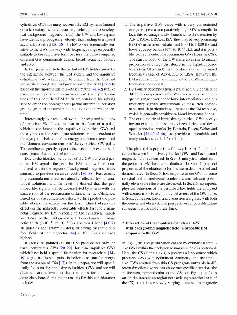
In Fig. 1, the EM perturbation caused by cylindrical impul-sive GWs within the background magnetic field is portrayed.Here, the CS (along z axis) represents a line-source whichproduces GWs with cylindrical symmetry, and the impul-sive GWs emitted from this CS propagate outwards in dif-ferent directions, so we can chose one specific direction (thex direction, perpendicular to the CS; see Fig. 1) to focuson. In the interaction region near axis (symmetrical axis ofthe CS), a static (or slowly varying quasi-static) magnetic

123

Eur. Phys. J. C (2014) 74:2998 Page 3 of 15 2998

Bz(0)

Interaction Region ofBackground Magnetic Field

Cosmic String

PerturbedEM Fields

x

Cylindrical GW Pulses

y

x

z

Fig. 1 Interaction between cylindrical impulsive GWs and backgroundmagnetic field. The cosmic string (alone z axis) is emitting GW pulsespropagating outwards perpendicularly to the CS, and we only focus onthe EM perturbation in the x direction specifically, the same hereinafter.The GW pulses will perturb the background magnetic field B(0)

z (point-ing to the z axis) and produce the perturbed EM fields propagating inthe x direction

field B(0)z is existing as an interactive background pointing to

the z direction. According to electrodynamical equations incurved spacetime [39,40], these cylindrical GW pulses willperturb this background magnetic field, and lead to perturbedEM fields (or in quantum language, signal photons) gener-ated within the region of background magnetic field; thenthe perturbed EM fields simultaneously and synchronouslypropagate in the identical direction to the impulsive GWsalong the x-axis.

As aforementioned in Sect. 1, the cosmic strings couldgenerate impulsive GWs [14–19] with broad frequency bands[3–7,21,33,34]. The key profiles of impulsive GWs are thepulse width ‘a’, the amplitude ‘A’ and its specific metric.Here, for convenience and clarity, we select the Einstein–Rosen metric to describe the cylindrical impulsive GWs.This well-known metric initially derived by Einstein andRosen based on general relativity [41,42,47] has been widelyresearched, as regards such pertinent issues as the energy-momentum pseudo-tensor [46–50]; its concise and succinctform could be advantageous to reveal the impulsive and cylin-drical symmetrical properties of GWs. Using the cylindricalpolar coordinates (ρ, ϕ, z) and time t , the Einstein–Rosenmetric of the general form of cylindrical GW can be writtenas [41,42,45] (c = 1 in natural units)

ds2 = e2(γ−ψ)(dt2 − dρ2)− e−2ψρ2dϕ2 − e2ψdz2; (1)

then the contravariant components of the metric tensor gμν

are

g00 = e2(ψ−γ ), g11 = −e2(ψ−γ ),g22 = −e2ψ, g33 = −e−2ψ. (2)

and we have√−g = e2(γ−ψ) (3)

here, the ψ and γ are functions of the distance ρ (which willbe denoted as ‘x’ in the coordinates after this section) and thetime t [41,42,45–47]. For the cylindrical impulsive GWs, areasonable and well-known form is the Weber–Wheeler (W-W) solution [45,46], namely:

ψ(ρ, t) = A

{1

[(a − i t)2 + ρ2] 12

+ 1

[(a + i t)2 + ρ2] 12

},

(4)

γ (ρ, t) = A2

2

{1

a2 − ρ2

[(a−i t)2+ρ2]2 − ρ2

[(a + i t)2+ρ2]2

− t2 + a2 − ρ2

a2[t4 + 2t2(a2 − ρ2)+ (a2 + ρ2)2] 12

}, (5)

where A and a are corresponding to the amplitude and pulsewidth of the cylindrical impulsive GW, respectively.

3 The perturbed EM fields produced by the impulsivecylindrical GWs in the background magnetic fields

When the cylindrical impulsive GWs described in Sect. 2[Eqs. (1) to (5)] propagate through the interaction region withbackground magnetic field B(0)

z , perturbed EM fields willbe generated. In this section, we will formulate a detailedcalculation on the exact forms of the perturbed EM fields.Notice that the word ‘exact’ here means that we utilize therigorous metric of cylindrical impulsive GW (Eq. 1) whichkeeps the cylindrical form, rather than the planar approx-imation usually used for weak fields as considered by thelinearized Einstein equation. Nonetheless, the cross sectionof the interaction between background magnetic field and theGW pulse is still very small, so the consideration of pertur-bation theory is reasonably suited to handle this case, and ascommonly accepted, some high order infinitesimals can beignored. However, manipulating without using the perturba-tion theory and without any sort of approximation to seekabsolutely strict results is also very interesting topic, and wewould investigate such issues in other works. Therefore, thetotal EM field tensor Fαβ can be expressed as two parts: thebackground static magnetic field F (0)

αβ , and the perturbed EM

fields F (1)αβ caused by the incoming impulsive GW; Because

of the cylindrical symmetry, it is always possible to describethe EM perturbation effect at the plane of y = 0 (i.e., thex–z plane, by use of a local Cartesian coordinate system, seeFig. 1, and the ‘x’ here substitutes for the distance ρ in Eqs.

123

2998 Page 4 of 15 Eur. Phys. J. C (2014) 74:2998

(4) and (5)), then Fαβ can be written as

Fαβ = F (0)αβ + F (1)

αβ

=

⎛⎜⎜⎜⎝

0 E (1)x E (1)

y E (1)z

−E (1)x 0 (−B(0)

z − B(1)z ) B(1)

y

−E (1)y (B(0)

z + B(1)z ) 0 −B(1)

x

−E (1)z −B(1)

y B(1)x 0

⎞⎟⎟⎟⎠.

(6)

Then, using the electrodynamical equations in curved space-time:

∇νFμν = 1√−g

∂

∂xν[√−ggμαgνβ(F (0)

αβ + F (1)αβ )] = 0,

∇αFμν + ∇νFαμ + ∇μFνα = 0,

where F (0)12 = −F (0)

21 = −B(0)z = −B(0) (7)

together with Eqs. (1)–(6), we have

μ = 0 ⇒ 2(γx − ψx )E(1)x − ∂E (1)

x

∂x= 0, (8)

μ = 1 ⇒ 2(ψt − γt )E(1)x + ∂E (1)

x

∂t= 0, (9)

μ = 2 ⇒ 2ψt E (1)y + ∂E (1)

y

∂t

+2ψx (B(0) + B(1)z )+ ∂B(1)

z

∂x= 0, (10)

μ = 3 ⇒ 2ψt E (1)z + ∂E (1)

z

∂t− 2ψx B(1)

y + ∂B(1)y

∂x= 0, (11)

∂B(1)x

∂x= 0,

∂B(1)x

∂t= 0,

∂E (1)z

∂x= ∂B(1)

y

∂t,∂E (1)

y

∂x= −∂B(1)

z

∂t. (12)

Here, γx , ψx , ψt , and γt stand for ∂γ∂x , ∂ψ

∂x , ∂ψ∂t , and ∂γ

∂t , andsimilarly hereinafter. So, by omitting second- and higher-order infinitesimal terms, it gives

∂2 E (1)y

∂x2 − ∂2 E (1)y

∂t2 = 2ψxt B(0) , (13)

∂2 B(1)z

∂x2 − ∂2 B(1)z

∂t2 = −2ψxx B(0) . (14)

Note that with Eqs. (8)–(12) and the initial conditions, wehave

E (1)y

∣∣∣∣t=0

= 0,∂E (1)

y

∂t

∣∣∣∣t=0

= −2ψx |t=0 · B(0) ,

B(1)z

∣∣∣∣t=0

= 0,∂B(1)

z

∂t

∣∣∣∣t=0

= 0. (15)

The other components, i.e., E (1)x , B(1)

x and E (1)z , B(1)

y haveonly null solutions. Non-vanishing EM components E (1)

y andB(1)

z are functions of x and t . To obtain their solutions, we

need to solve the set of second-order non-homogeneous par-tial differential equations in Eqs. (13)–(15), and utilizing thed’Alembert formula, we can express the solutions in analyt-ical form [51]:

E (1)y = 1

2

∫ x+t

x−tH(ξ)dξ

+1

2

∫ t

0

∫ x+(t−τ)

x−(t−τ)F(ξ, τ )dξdτ, (16)

B(1)z = 1

2

∫ t

0

∫ x+(t−τ)

x−(t−τ)G(ξ, τ )dξdτ, (17)

where

H(ξ) = −2ψξ |t=0 · B(0) ,

F(ξ, τ ) = −2ψξτ B(0) ,

G(ξ, τ ) = 2ψξξ B(0) . (18)

By the integral from Eq. (16), one finds

1

2

∫ x+t

x−tH(ξ)dξ = −1

∫ x+t

x−tψξ |t=0 · B(0)dξ

= 2AB(0)

{1

[(x − t)2 + a2] 12

− 1

[(x + t)2 + a2] 12

}(19)

and, similarly,

1

2

∫ t

0

∫ x+(t−τ)

x−(t−τ)F(ξ, τ )dξdτ

= −AB(0)

{∫ t

0

τ + ia

[(x + t − τ)2 + (a − i t)2] 32

dτ

+∫ t

0

τ − ia

[(x + t − τ)2 + (a + i t)2] 32

dτ

−∫ t

0

τ + ia

[(x − t + τ)2 + (a − i t)2] 32

dτ

−∫ t

0

τ − ia

[(x − t + τ)2 + (a + i t)2] 32

dτ

}(20)

and

1

2

∫ t

0

∫ x+(t−τ)

x−(t−τ)G(ξ, τ )dξdτ

= −AB(0)

{∫ t

0

x + t − τ

[(x + t − τ)2 + (a − iτ)2] 32

dτ

+∫ t

0

x + t − τ

[(x + t − τ)2 + (a + iτ)2] 32

dτ

123

Eur. Phys. J. C (2014) 74:2998 Page 5 of 15 2998

−∫ t

0

x − t + τ

[(x − t + τ)2 + (a − iτ)2] 32

dτ

−∫ t

0

x − t + τ

[(x − t + τ)2 + (a + iτ)2] 32

dτ

}. (21)

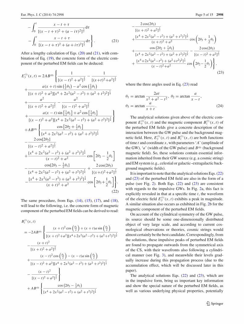
After a lengthy calculation of Eqs. (20) and (21), with com-bination of Eq. (19), the concrete form of the electric com-ponent of the perturbed EM fields can be deduced:

E (1)y (x, t) = 2AB(0)

{1

[(x − t)2 + a2] 12

− 1

[(x+t)2+a2] 12

+ a(x + t) sin( 1

2θ1) − a2 cos

( 12θ1

)[(x + t)2 + a2][x4 + 2x2(a2 − t2)+ (a2 + t2)2] 1

4

+ a2

[(x + t)2 + a2] 32

− a2

[(x − t)2 + a2] 32

+ a(x − t) sin[ 1

2θ1] + a2 cos

[ 12θ1

][(x − t)2 + a2][x4 + 2x2(a2 − t2)+ (a2 + t2)2] 1

4

}

+AB(0)

{cos

[2θ2 + 1

2θ1]

[x4 + 2x2(a2 − t2)+ (a2 + t2)2] 14

− 2 cos[2θ2][(x − t)2 + a2] 1

2

+[x4 + 2x2(a2 − t2)+ (a2 + t2)2] 14

(x − t)2 + a2 cos

[2θ2 − 1

2θ1

]

− cos[2θ3 − 12θ1]

[x4 + 2x2(a2 − t2)+ (a2 + t2)2] 14

+ 2 cos(2θ3)

[(x+t)2+a2] 12

−[x4 + 2x2(a2 − t2)+ (a2 + t2)2] 14

(x + t)2 + a2 cos

[2θ3+ 1

2θ1

]}.

(22)

The same procedure, from Eqs. (14), (15), (17), and (18),will lead to the following, i.e. the concrete form of magneticcomponent of the perturbed EM fields can be derived to read:

B(1)z (x, t)

= −2AB(0)

⎧⎨⎩

(x + t)2 cos(θ12

)+ (x + t)a sin

(θ12

)[(x + t)2+a2][x4+2x2(a2−t2)+ (a2+t2)2] 1

4

− (x + t)2

[(x + t)2 + a2] 32

+(x − t)2 cos

(θ12

)− (x − t)a sin

(θ12

)[(x − t)2 + a2][x4 + 2x2(a2 − t2)+ (a2 + t2)2] 1

4

− (x − t)2

[(x − t)2 + a2] 32

⎫⎬⎭

+ AB(0)

{cos

(2θ3 − 1

2 θ1)

[x4 + 2x2(a2 − t2)+ (a2 + t2)2] 14

− 2 cos(2θ3)

[(x + t)2 + a2] 12

+[x4 + 2x2(a2 − t2)+ (a2 + t2)2] 14

(x + t)2 + a2 cos

(2θ3 + 1

2θ1

)

+ cos(2θ2 + 1

2 θ1)

[x4 + 2x2(a2 − t2)+ (a2 + t2)2] 14

− 2 cos(2θ2)

[(x − t)2 + a2] 12

+ [x4+2x2(a2−t2)+ (a2+t2)2] 14

(x − t)2+a2 cos

(2θ2− 1

2θ1

)},

(23)

where the three angles used in Eq. (23) read

θ1 = arctan2at

x2 + a2 − t2 , θ2 = arctana

x − t,

θ3 = arctana

x + t. (24)

The analytical solutions given above of the electric com-ponent E (1)

y (x, t) and the magnetic component B(1)z (x, t) of

the perturbed EM fields give a concrete description of theinteraction between the GW pulse and the background mag-netic field. Here, E (1)

y (x, t) and B(1)z (x, t) are both functions

of time t and coordinate x , with parameters ‘A’ (amplitude ofthe GW), ‘a’ (width of the GW pulse) and B(0) (backgroundmagnetic field). So, these solutions contain essential infor-mation inherited from their GW source (e.g. a cosmic string)and EM system (e.g., celestial or galactic–extragalactic back-ground magnetic fields).

It is important to note that the analytical solutions Eqs. (22)and (23) of the perturbed EM field are also in the form of apulse (see Fig. 2). Both Eqs. (22) and (23) are consistentwith regards to the impulsive GWs. In Fig. 2a, this fact isexplicitly revealed in that at a specific time t , the waveformof the electric field E (1)

y (x, t) exhibits a peak in magnitude.A similar situation also occurs as exhibited in Fig. 2b for themagnetic component of the perturbed EM fields.

On account of the cylindrical symmetry of the GW pulse,its source should be some one-dimensionally distributedobject of very large scale, and according to current cos-mological observations or theories, cosmic strings wouldalmost certainly be the best candidate. Correspondingly, fromthe solutions, these impulsive peaks of perturbed EM fieldsare found to propagate outwards from the symmetrical axisof the CS, with their wavefronts also following a cylindri-cal manner (see Fig. 3), and meanwhile their levels grad-ually increase during this propagation process (due to theaccumulation effect, which will be discussed later in thispaper).

The analytical solutions Eqs. (22) and (23), which arein the impulsive form, bring us important key informationand show the special nature of the perturbed EM fields, aswell as various underlying physical properties, potentially

123

2998 Page 6 of 15 Eur. Phys. J. C (2014) 74:2998

x m

E (x,t),(v/m)y

(a)

- 2. x10-1

- 1. x10-1

0

1. x10-1

2. x10-1

3. x10-1

11.5 15.5 19.5 23.5 27.57.5

B (x,t),(Tesla)z

(b)

x m

4 8 12 16 200- 6.x10 -10- 4.x10 -10- 2.

0-10

2.x10 -104.x10 -106.x10 -108.x10 -10

x10

(1)

(1)

Fig. 2 Typical examples of electric and magnetic components of per-turbed impulsive EM fields in the region near axis. According to Eq.(22), a a representative electric component E (1)

y (x, t) of the impulsiveEM field produced by the interaction between cylindrical GW pulse(width a = 0.4 m, amplitude h ∼10−21; here we denote ‘h’ instead of‘A’ as the amplitude in the SI units, similarly hereinafter) and higherbackground magnetic field (1011 Tesla, could be generated from celes-tial bodies [44], the same hereinafter). Here we assume h ∼10−21 (sim-ilarly in the figures below), and the detailed reason for this choice maybe found in Sect. 5. In the same way, according to Eq. (23), b a typicalmagnetic component B(1)

z (x, t) of perturbed EM fields (with GW widtha = 0.4 m, h ∼10−21) in the region of the near axis. Both electric andmagnetic components of the perturbed impulsive EM fields are in theform of a pulse, consistent with the GW pulses. This figure is plottedassuming SI units

Fig. 3 Wavefronts of the perturbed EM fields in background magneticfield. The plot generated above is based upon Eq. (22), and it demon-strates the cylindrical wavefronts of the EM fields as perturbed by thecylindrical GW pulses

observable effects, and asymptotic behaviors. These aspectswill consequently be analyzed and discussed in full in thefollowing sections.

4 Physical properties of analytical solutionsof the perturbed EM fields

With the analytical solutions of the perturbed EM fields asrepresented in the above section, some of their interestingproperties may be studied in detail. For example, what isthe relationship between the given width-amplitude of theperturbed EM fields and the width-amplitude of the GWpulse? Secondly, is there any accumulation effect (consis-tent with previous work in the literature on the EM respondto GWs) of the interaction between the GW pulses and thebackground magnetic field since the GWs and the perturbedEM fields share the same velocity (speed of light)? In addi-tion we also ask what the spectrum is of the amplitude ofthe perturbed EM field and how it is related to the param-eters of the corresponding GW pulse. For convenience, weuse SI units in this section and Sect. 5. The details are asfollows:

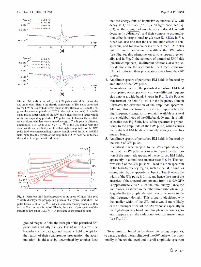
1. The relationship between the parameters of the GWpulse and the impulsive features of the perturbed EMfield.From Eq. (22), it is simply deduced that the amplitudeh (here ‘h’ is written in place of ‘A’ as the amplitude inSI units) of the GW pulse and the background magneticfield, B(0), contribute linear factors for the perturbedEM field which we designate in this paper as E (1)

y (x, t).So E (1)

y (x, t) varies according to h proportionally (seeFig. 4b). However, the width ‘a’ of a GW pulse playsa more complex role in Eq. (22), but we find that thewidth ’a’ is still positively correlated to the width of theperturbed EM fields, i.e., a smaller width of the GWpulse leads to a smaller width of the perturbed EM field(see Fig. 4a), and the EM pulse with a narrower peak isfound to have a larger strength and a more concentratedenergy.

2. Propagating velocity of perturbed EM pulses.The information as regards the propagating velocity ofthe GW as the speed of light is naturally included in thedefinition of the metric (Eqs. (1)–(5)). In the same way,EM pulses caused by the GW pulse also are propagat-ing at the speed of light due to EM theory in free space(but also in curved spacetime) [39,40]. For intuitive rep-resentation, we exhibit this property in Fig. 5, whichillustrates the exact given field contours of E (1)

y (x, t) atdifferent times from t = 0 to t = 20

c s.3. Accumulation effect due to the identical propagating

velocity of EM pulses and GW pulse.As mentioned above, we see that the perturbed EM fieldspropagate at the speed of light synchronously with theGW pulse; then the perturbed EM fields caused by theinteraction between GW pulse and background magneticfield will accumulate. So, in the region with a given back-

123

Eur. Phys. J. C (2014) 74:2998 Page 7 of 15 2998

5.x10-1

(a)

0

2.5 x10 -1

-2.5 x10-1

4 5 6 7 8 9

x m

E (v/m)y

a = 0.2 ma = 0.3 ma = 0.4 ma = 0.6 m

-5.x10 -2

1.x10 -1

1.5 x10 -1

-1.x10 -1

-1.5 x10 -1

0

2 4 6 8 10 12

x m

E (v/m)y

h = 0.5 h0

h = 1.0 h0

h = 1.5 h0

h = 2.0 h0

(b)

5.x10 -2

(1)

(1)

Fig. 4 EM fields perturbed by the GW pulses with different widthsand amplitudes. Here, a the electric components of EM fields perturbedby the GW pulses with different pulse widths (from a = 0.2 to 0.6 m,given the same amplitude ∼10−21 in the region near axis). It is indi-cated that a larger width of the GW pulse gives rise to a larger widthof the corresponding perturbed EM pulse, but it also results in a flat-ter waveform with less concentrated energy. b The impact of differentamplitudes (h = 0.5 to 2 h0, h0 ∼10−21) of the GW pulses with thesame width, and explicitly we find that higher amplitudes of the GWpulse lead to a correspondingly greater amplitude of the perturbed EMfield. Note that the growth of the amplitude of GW does not influencethe width of the perturbed EM pulse

x(m)

time(s)

Ey(x,t)(v/m)

E ( )20, 20/cy

-5. x10-9

05. x10-9

1. x10-8

20/c

4 8 12 16 20 24 28

5/c

10/c

15/c

x10-8-1. 0

(1)

Fig. 5 Perturbed EM field propagates at the speed of light. This plotvisually displays the propagating process of a typical perturbed EM

pulse from t = 0 to t = 20c s, which is linearly moving from x = 0 m

to x = 20 m during this period. That is, the speed of propagation of theperturbed EM pulse is 20/ 20

c = c, the same as the speed of light

ground magnetic field, the strength of the perturbed EMpulse will gradually rise (see Fig. 6) until it leaves theboundary of the background magnetic field. Except forthe reason of their synchronous propagation, the accu-mulation should also be determined by another fact:

that the energy flux of impulsive cylindrical GW willdecay as 1/distance (or ∼1/x on light cone, see Eq.(33), so the strength of impulsive cylindrical GW willdecay as 1/

√distance), and their composite accumula-

tion effect is proportional to√

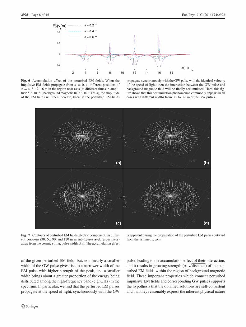
x (see Eq. (28)). In Fig.6, we can also find that the accumulation effect is con-spicuous, and for diverse cases of perturbed EM fieldswith different parameters of width of the GW pulses(see Fig. 6), this phenomenon always appears gener-ally, and in Fig. 7, the contours of perturbed EM fields(electric component), in different positions, also explic-itly demonstrate the accumulated perturbed impulsiveEM fields, during their propagating away from the GWsource.

4. Amplitude spectra of perturbed EM fields influenced byamplitude of the GW pulse.As mentioned above, the perturbed impulsive EM fieldis comprised of components with very different frequen-cies among a wide band. Shown in Fig. 8, the Fouriertransform of the field E (1)

y (x, t) in the frequency domainillustrates the distribution of the amplitude spectrum.Although this spectrum decreases as it approaches thehigh-frequency range, it still remains available at a levelin the neighborhood of the GHz band. Overall, it is indi-cated that (see Fig. 8) the level of the spectrum is propor-tional to the amplitude of the GW pulse, which causesthe perturbed EM fields, commonly among entire fre-quency bands.

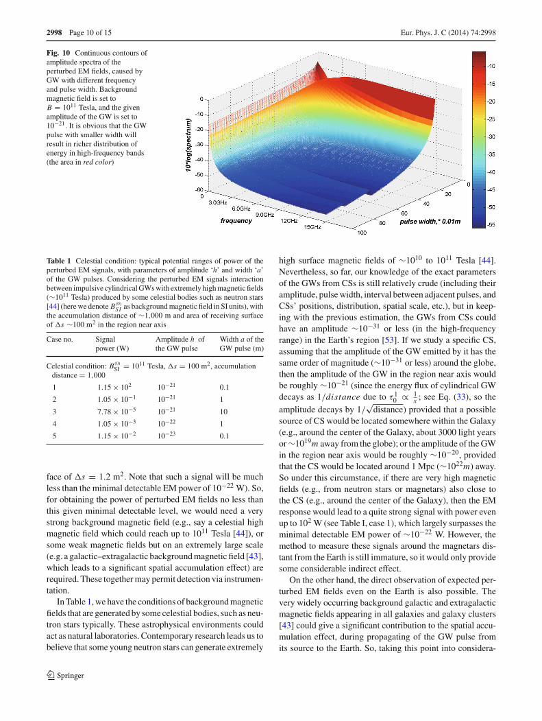
5. Amplitude spectra of perturbed EM fields influenced bythe width of GW pulse.In contrast to what happens to the GW amplitude h, thewidth of the GW pulse acts so as to impact the distribu-tion of the amplitude spectra of the perturbed EM fields,apparently in a nonlinear manner (see Fig. 9). The nar-row width of the GW pulse will lead to a rich spectrumin the high-frequency region, such as the GHz band, asexemplified by the upper-left subplot of Fig. 9, where thewidth of the GW pulse is 0.1 m, and hence the sum of theenergies of the spectral components from 1 to 9.9 GHzis approximately 24.5 % of the total energy. Once thewidth rises, as shown in the other three subplots in Fig.9, gradually the amplitude spectra will decrease in thehigh-frequency domain. This property elucidates whythe smaller width of the GW pulse would more likelycause a stronger effect of the EM response especially inthe high-frequency band, and this phenomenon is gen-erally appearing in the wide continuous parameter range(see Fig. 10).

To summarize, based on the above interesting properties,we can argue that: the amplitude of the GW pulse will propor-tionally influence the level and overall amplitude spectrum

123

2998 Page 8 of 15 Eur. Phys. J. C (2014) 74:2998

a = 0.6 m

a = 0.4 m

a = 0.2 mE (v/m)y

x(m)2 4 8 216 10 14 16 18

-0.5

0

1.0

0.5

(1)

Fig. 6 Accumulation effect of the perturbed EM fields. When theimpulsive EM fields propagate from x = 0, at different positions ofx = 4, 8, 12, 16 m in the region near axis (at different times, t, ampli-tude h ∼10−21, background magnetic field ∼1011 Tesla), the amplitudeof the EM fields will then increase, because the perturbed EM fields

propagate synchronously with the GW pulse with the identical velocityof the speed of light; then the interaction between the GW pulse andbackground magnetic field will be finally accumulated. Here, this fig-ure shows that this accumulation phenomenon commonly appears in allcases with different widths from 0.2 to 0.6 m of the GW pulses

Fig. 7 Contours of perturbed EM fields(electric component) in differ-ent positions (30, 60, 90, and 120 m in sub-figures a–d, respectively)away from the cosmic string, pulse width: 5 m. The accumulation effect

is apparent during the propagation of the perturbed EM pulses outwardfrom the symmetric axis

of the given perturbed EM field, but, nonlinearly a smallerwidth of the GW pulse gives rise to a narrower width of theEM pulse with higher strength of the peak, and a smallerwidth brings about a greater proportion of the energy beingdistributed among the high-frequency band (e.g. GHz) in thespectrum. In particular, we find that the perturbed EM pulsespropagate at the speed of light, synchronously with the GW

pulse, leading to the accumulation effect of their interaction,and it results in growing strength (∝ √

distance) of the per-turbed EM fields within the region of background magneticfield. These important properties which connect perturbedimpulsive EM fields and corresponding GW pulses supportsthe hypothesis that the obtained solutions are self-consistentand that they reasonably express the inherent physical nature

123

Eur. Phys. J. C (2014) 74:2998 Page 9 of 15 2998

of the EM response to cylindrical impulsive GW. Clearly, themagnetic component (Eq. (23)) of the perturbed EM field hassimilar properties.

Frequency (GHz)

Fourier transform of signal (E component)

Spe

ctru

m o

f E fi

eld

ampl

itude

(dB

/Hz)

0 5 10 15-90

-80

-70

-60

-50

-40

-30

-20

-10

h ~ 10 -21

h ~ 10 -22

h ~ 10 -23

h ~ 10 -24

i

ii

iii

iv

i

ii

iii

iv

Fig. 8 Amplitude spectra of perturbed EM fields caused by the GWpulses with different amplitudes. This figure demonstrates the ampli-tude spectra of perturbed EM fields (electric component) caused by theGW pulses with different amplitudes from ∼10−21 to ∼10−24 (withidentical width of a = 0.5 m). For all cases, the spectra will decay asthe frequency grows, but it will still remain at a considerable level evenover the GHz band. It reflects the proportional relationship between theoverall level of spectrum among all frequency region and the amplitudeof GW pulse. The unit ‘dB’ here means 10 × log10()

5 Electromagnetic response to the GW pulse by celestialor cosmological background magnetic fields and itspotentially observable effects

The analytical solutions Eqs. (22) and (23) of perturbedEM fields provide helpful information for studying the CSs,impulsive cylindrical GWs, and relevant potentially observ-able effects. According to classical electrodynamics, thepower flux at a receiving surface s of the perturbed EMfields may be expressed as

U = 1

2μ0Re[E (1)∗

y (x, t) · B(1)z (x, t)] s (25)

The observability of the perturbed EM fields will be deter-mined concurrently by a lot of parameters of both GW pulseand other observation condition, such as the amplitude andwidth of the GW pulse, the strength of background magneticfield, the accumulation length (distance from GW source toreceiving surface), the detecting technique for weak pho-tons, the noise issue(and so on). Under conditions of cur-rent technology, the detectable minimal EM power would be∼10−22W in the 1-Hz bandwidth [52], so we could approx-imately assume the detectable minimal EM power for ourcase in this paper is the same order of magnitude. Also, thepower of the perturbed EM fields is too weak by only usingcurrent laboratory magnetic field (e.g., strength of ∼20 Tesla,accumulation distance of = 3 m and area of receiving sur-

Fig. 9 Amplitude spectra ofperturbed EM fields caused bythe GW pulses with differentwidths. In the four subplotsinvolving amplitude spectra ofperturbed EM fields, thecorresponding GW pulses havedifferent widths of 0.1, 0.5, 1and 2 m, respectively (allamplitudes are here ∼10−21). Itis manifestly obvious that theGW pulse with smaller width(such as 0.1 m), will definitelyresult in much more energydistributed in the high-frequencybands of the perturbed EMfields. Also, inversely, the GWpulse with larger width (such as2 m), will lead to conditions forobserving a very dramaticattenuation of power of theperturbed EM fields in the highfrequency bands. The unit ‘dB’here means 10 × log10()

Spe

ctru

m o

f E fi

eld

ampl

itude

(dB

/Hz)

Frequency (GHz)

Fourier transform of signal (E component)

0 5 10 15-60

-50

-40

-30

-20

-10

0 5 10 15-60

-50

-40

-30

-20

-10

0 5 10 15-60

-50

-40

-30

-20

-10

0 5 10 15-60

-50

-40

-30

-20

-10

pulse Width = 0.1m pulse Width = 0.5m

pulse Width = 1 m pulse Width = 2 m

123

2998 Page 10 of 15 Eur. Phys. J. C (2014) 74:2998

Fig. 10 Continuous contours ofamplitude spectra of theperturbed EM fields, caused byGW with different frequencyand pulse width. Backgroundmagnetic field is set toB = 1011 Tesla, and the givenamplitude of the GW is set to10−21. It is obvious that the GWpulse with smaller width willresult in richer distribution ofenergy in high-frequency bands(the area in red color)

Table 1 Celestial condition: typical potential ranges of power of theperturbed EM signals, with parameters of amplitude ‘h’ and width ‘a’of the GW pulses. Considering the perturbed EM signals interactionbetween impulsive cylindrical GWs with extremely high magnetic fields(∼1011 Tesla) produced by some celestial bodies such as neutron stars[44] (here we denote B(0)

SI as background magnetic field in SI units), withthe accumulation distance of ∼1,000 m and area of receiving surfaceof s ∼100 m2 in the region near axis

Case no. Signalpower (W)

Amplitude h ofthe GW pulse

Width a of theGW pulse (m)

Celestial condition: B(0)SI = 1011 Tesla, s = 100 m2, accumulation

distance = 1,000

1 1.15 × 102 10−21 0.1

2 1.05 × 10−1 10−21 1

3 7.78 × 10−5 10−21 10

4 1.05 × 10−3 10−22 1

5 1.15 × 10−2 10−23 0.1

face of s = 1.2 m2. Note that such a signal will be muchless than the minimal detectable EM power of 10−22 W). So,for obtaining the power of perturbed EM fields no less thanthis given minimal detectable level, we would need a verystrong background magnetic field (e.g., say a celestial highmagnetic field which could reach up to 1011 Tesla [44]), orsome weak magnetic fields but on an extremely large scale(e.g. a galactic–extragalactic background magnetic field [43],which leads to a significant spatial accumulation effect) arerequired. These together may permit detection via instrumen-tation.

In Table 1, we have the conditions of background magneticfields that are generated by some celestial bodies, such as neu-tron stars typically. These astrophysical environments couldact as natural laboratories. Contemporary research leads us tobelieve that some young neutron stars can generate extremely

high surface magnetic fields of ∼1010 to 1011 Tesla [44].Nevertheless, so far, our knowledge of the exact parametersof the GWs from CSs is still relatively crude (including theiramplitude, pulse width, interval between adjacent pulses, andCSs’ positions, distribution, spatial scale, etc.), but in keep-ing with the previous estimation, the GWs from CSs couldhave an amplitude ∼10−31 or less (in the high-frequencyrange) in the Earth’s region [53]. If we study a specific CS,assuming that the amplitude of the GW emitted by it has thesame order of magnitude (∼10−31 or less) around the globe,then the amplitude of the GW in the region near axis wouldbe roughly ∼10−21 (since the energy flux of cylindrical GWdecays as 1/distance due to τ 1

0 ∝ 1x ; see Eq. (33), so the

amplitude decays by 1/√

distance) provided that a possiblesource of CS would be located somewhere within the Galaxy(e.g., around the center of the Galaxy, about 3000 light yearsor ∼1019m away from the globe); or the amplitude of the GWin the region near axis would be roughly ∼10−20, providedthat the CS would be located around 1 Mpc (∼1022m) away.So under this circumstance, if there are very high magneticfields (e.g., from neutron stars or magnetars) also close tothe CS (e.g., around the center of the Galaxy), then the EMresponse would lead to a quite strong signal with power evenup to 102 W (see Table I, case 1), which largely surpasses theminimal detectable EM power of ∼10−22 W. However, themethod to measure these signals around the magnetars dis-tant from the Earth is still immature, so it would only providesome considerable indirect effect.

On the other hand, the direct observation of expected per-turbed EM fields even on the Earth is also possible. Thevery widely occurring background galactic and extragalacticmagnetic fields appearing in all galaxies and galaxy clusters[43] could give a significant contribution to the spatial accu-mulation effect, during propagating of the GW pulse fromits source to the Earth. So, taking this point into considera-

123

Eur. Phys. J. C (2014) 74:2998 Page 11 of 15 2998

0 1.

0 2.

0.3

.40

0 5.

Pulse width(m)0

5 x10 -22

1 x10 -21

GW amplitude h

0

5x10-23

1x10-22

sign

al p

ower

(W

att)

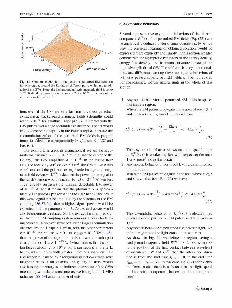
Fig. 11 Continuous 3D plot of the power of perturbed EM fields (infar axis region, around the Earth), by different pulse width and ampli-tude of the GWs. Here, the background galactic magnetic field is set to10−9 Tesla, the accumulation distance is 2.8 × 1019 m, the area of thereceiving surface is 5 m2

tion, even if the CSs are very far from us, these galactic–extragalactic background magnetic fields (strengths couldreach ∼10−9 Tesla within 1 Mpc [43]) will interact with theGW pulses over a huge accumulative distance. Then it wouldlead to observable signals in the Earth’s region, because theaccumulation effect of the perturbed EM fields is propor-tional to

√distance asymptotically (∼√

x ; see Eq. (28) andFig. (6)).

For example, as a rough estimation, if we set the accu-mulation distance ∼2.8 × 1019 m (e.g. around center of theGalaxy), the GW amplitude h ∼10−21 in the region nearaxis, the receiving surface s ∼5 m2, the GW pulse widtha ∼5 cm, and the galactic–extragalactic background mag-netic field BGMF ∼10−9 Tesla, then the power of the signal inthe Earth’s region would reach up to 1.3×10−22 W (see Fig.11; it already surpasses the minimal detectable EM powerof 10−22 W, and it means that the photon flux is approxi-mately 112 photons per second in the GHz band). Besides, ifthis weak signal can be amplified by the schemes of the EMcoupling [36,37,54], then a higher signal power would beexpected, and the parameters of h, s, a, and BGMF wouldalso be enormously relaxed. Still, to extract the amplified sig-nal from the EM coupling system remains a very challeng-ing problem. Moreover, if we consider a larger accumulationdistance around 1 Mpc ∼1022 m, with the other parametersh ∼10−20, s ∼1 m2, a ∼0.1 m, BGMF ∼10−9 Tesla [43],then the power of the signal on the Earth would reach up toa magnitude of 1.2 × 10−19 W (which means that the pho-ton flux is about 4.4 × 104 photons per second in the GHzband), which comes with greater direct observability. ThisEM response, caused by background galactic–extragalacticmagnetic fields in all galaxies and galaxy clusters, wouldalso be supplementary to the indirect observation of the GWsinteracting with the cosmic microwave background (CMB)radiation [55–59] or some other effects.

6 Asymptotic behaviors

Several representative asymptotic behaviors of the electriccomponent E (1)

y (x, t) of perturbed EM fields (Eq. (22)) canbe analytically deduced under diverse conditions, by whichway the physical meaning of obtained solution would beexpressed more explicitly and simply. In this section we alsodemonstrate the asymptotic behaviors of the energy density,energy flux density, and Riemann curvature tensor of theimpulsive cylindrical GW. The self-consistency, commonal-ities, and differences among these asymptotic behaviors ofboth GW pulse and perturbed EM fields will be figured out.For convenience, we use natural units in the whole of thissection.

1. Asymptotic behavior of perturbed EM fields in space-like infinite region.When the EM pulses propagate in the area where x � tand x � a (width), from Eq. (22) we have

E (1)y (x, t) → AB(0)

[4t

x2 − 12a2t

x4

]∝ 4AB(0)

t

x2 .

(26)

This asymptotic behavior shows that, at a specific timet , E (1)

y (x, t) is weakening fast with respect to the term1/distance2 along the x-axis.

2. Asymptotic behavior of perturbed EM fields in time-likeinfinite region.When the EM pulses propagate in the area where x tand t � a, also from Eq. (22) we have

E (1)y (x, t) → AB(0)

4x

t2 − 4AB(0)a2 1

t3 ∝ 4AB(0)x

t2 .

(27)

This asymptotic behavior of E (1)y (x, t) indicates that,given a specific position x , EM pulses will fade away as1/t2.

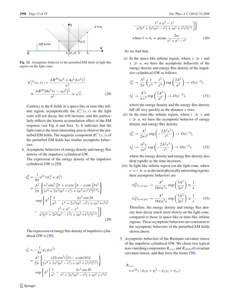
3. Asymptotic behavior of perturbed EM fields in light-likeinfinite region (on the light cone, i.e. x = t � a).As shown in Fig. 12, we define the region having abackground magnetic field B(0) is x � x0, where x0

is the position of the first contact between wavefrontof impulsive GW and B(0), then the interaction dura-tion is from the start time tmin = 0, to the end timetmax = x − x0 = x . In this case, Eq. (22) approachesthe form (notice there is a factor c of the light speedin the electric component, but c=1 in the natural unitshere)

123

2998 Page 12 of 15 Eur. Phys. J. C (2014) 74:2998

GW pulse

x0 0(x , )0 x1

x

x-t=x0

(x,t)

0

t

x

Fig. 12 Asymptotic behavior of the perturbed EM fields in light-likeregion (on the light cone)

E (1)y (x, t) → AB(0)(a4 + 4a2 x2)14

a2

≈

AB(0)[4a2(x − x0)2] 1

4

a2 ∝ √x . (28)

Contrary to the E fields in a space-like or time-like infi-nite region, asymptotically the E (1)

y (x, t) on the lightcone will not decay, but will increase, and this particu-larly reflects the known accumulation effect of the EMresponse (see Fig. 6 and Sect. 3). It indicates that thelight cone is the most interesting area to observe the per-turbed EM fields. The magnetic component B(1)

z (x, t) ofthe perturbed EM fields has similar asymptotic behav-iors.

4. Asymptotic behaviors of energy density and energy fluxdensity of the impulsive cylindrical GW.The expression of the energy density of the impulsivecylindrical GW is [50]

τ 00 = 1

8πe2γ (ψ2

x + ψ2t )

= A2

2π

{x2 cos2 3

2θ + (t cos 32θ − a sin 3

2θ)2

[x4 + 2x2(a2−t2)+ (a2+t2)2]3/2)

}

· exp

{A2

[1

a2 − 2x2 cos 2θ

x4 + 2x2(a2−t2)+ (a2+t2)2

− t2 + a2 − x2

a2[t4 + 2t2(a2 − t2)+ (a2+t2)2]1/2

]}.

(29)

The expression of energy flux density of impulsive cylin-drical GW is [50]

τ 10 = − 1

4πψρψt e

2γ

= A2

2π

{x[2t cos2( 3

2θ)− a sin(3θ)][x4 + 2x2(a2 − t2)+ (a2 + t2)2]3/2)

}

· exp

{A2

[1

a2 − 2x2 cos 2θ

x4 + 2x2(a2 − t2)+ (a2 + t2)2

− t2 + a2 − x2

a2[t4 + 2t2(a2 − t2)+ (a2 + t2)2]1/2

]}

where θ = θ1 = arctan2at

x2 + a2 − t2 . (30)

So we find that:

(i) In the space-like infinite region, where x � t andx � a, we have the asymptotic behaviors of theenergy density and energy flux density of the impul-sive cylindrical GW as follows:

τ 00 → A2

2π

(1

x4 + t2

x6

)exp

(2A2

a2

)→ O(x−4),

τ 10 → A2t

πx5exp

(2A2

a2

)→ O(x−5), (31)

where the energy density and the energy flux densityfall off very quickly as the distance x rises.

(ii) In the time-like infinite region, where t � x andt � a, we have the asymptotic behavior of energydensity and energy flux density:

τ 00 → A2

2π t4 exp

(−2A2x2

t4

)→ O(t−4),

τ 10 → A2x

π t5exp

(−2A2x2

t4

)→ O(t−5), (32)

where the energy density and energy flux density alsodrop rapidly as the time increases.

(iii) In light-like infinite region (on the light cone, wherex = t � a, as the most physically interesting region),their asymptotic behaviors are

(τ 00 )x=t�a → A2

16πa3xexp

(3A2

2a2

)∝ 1

x,

(τ 10 )x=t�a → A2

16πa3xexp

(3A2

2a2

)∝ 1

x. (33)

Therefore, the energy density and energy flux den-sity here decay much more slowly on the light cone,compared to those in space-like or time-like infiniteregions. These asymptotic behaviors are consistent tothe asymptotic behaviors of the perturbed EM fieldsshown above.

5. Asymptotic behaviors of the Riemann curvature tensorof the impulsive cylindrical GW. We chose two typicalnon-vanishing components Rxzxz and Ry0y0 of covariantcurvature tensor, and they have the forms [50]

Rxzxz

= e2ψ(−ψtγt + ψ2t − ψxγx + ψxx )

123

Eur. Phys. J. C (2014) 74:2998 Page 13 of 15 2998

= e2ψ

{−2A cos 3

2 θ

r3/4 + 6Ax2 cos 52 θ

r5/4

+16A3x2 cos 32 θ

[x2 cos2 3

2 θ+2(x cos 32 θ−a sin 3

2 θ)2]

r9/4

+4A2[2x2 cos2 3

2 θ+(x cos 32 θ−a sin 3

2 θ)2]

r3/2

}, (34)

where r = x4 + 2x2(a2 − t2) + (a2 + t2)2, the samehereinafter, and

Ry0y0

= −e−2ψ(−ψt t − ψtγt + (γx − ψx )/x − ψxγx + ψ2x )

= −e−2ψ

⎧⎨⎩4A cos 3

2 θ

r3/4 +6A

[(t2−a2) cos 5

2 θ−at sin 52 θ

]r5/4

−8A3x2 cos2 32 θ

[x2 cos2 3

2 θ−(t cos 32 θ−a sin 3

2 θ)2]

r9/4

+4A2[2x2 cos2 3

2 θ + (t cos 32 θ − a sin 3

2 θ)2]

r3/2

⎫⎬⎭ , (35)

then we find that:

(i) in the space-like infinite region where x � t andx � a, asymptotically it gives

Rxzxz →(

4A

x3 + 12A2

x4 + 48A3

x5

)exp

(4A

x

)

→ 4A

x3 exp

(4A

x

)→ O

(1

x3

)(36)

and

Ry0y0 → −[

4A

x3 + 8A2

x4 + 6A(t2 − a2)− 8A3

x5

]

× exp

(−4A

x

)

→ −4A

x3 exp

(−4A

x

)→ O

(1

x3

); (37)

(ii) in the time-like infinite region, where t � x andt � a, we have the asymptotic behaviors

Rxzxz →(−2A

t3 + 6Ax2

t5+ 12A2x2

t6 + 48A3x4

t9

)

× exp

(4A

t

)

→ −2A

t3 exp

(4A

t

)→ O

(1

t3

)(38)

and

Ry0y0 →(

10A

t3 + 4A2

t4 + 8A3x2

t7

)

× exp

(−4A

t

)

→ −10A

t3 exp

(−4A

t

)→ O

(1

t3

); (39)

(iii) in the light-like infinite region (on the light cone),where x = t � a, their asymptotic behaviors are

Rxzxz → −3

4

(A

a5/2x1/2+ A3

a9/2x1/2

)

× exp

( −2A

a1/2x1/2

)∝ 1

x1/2 (40)

and

Ry0y0 →(

3A

4a5/2x1/2+ 3A2

4a3x+ A

a3/2x3/2

)

× exp

(2A

a1/2x1/2

)

→ 3A

4a5/2x1/2exp

(2A

a1/2x1/2

)∝ 1

x1/2 .

(41)

Apparently, these components of the Riemann curvaturetensor decrease much more slowly on the light cone (themost interesting region and the particular one with therichest observable information), as compared to those inthe space-like or time-like infinite regions where theyattenuate very rapidly. This characteristic agrees wellwith the asymptotic behaviors of the energy density,energy flux density of the impulsive cylindrical GW, andasymptotic behaviors of the perturbed EM fields. Partic-ularly, only on the light cone, the perturbed EM fieldswill be growing instead of declining, which speciallyreflects the spatial accumulation effect. All of the aboveasymptotic behaviors play supporting roles in furthercorroboration of the self-consistency and reasonablenessof the obtained solutions.

7 Conclusion and discussion

First, in the frame of general relativity, based upon the elec-trodynamical equations in curved spacetime, utilizing thed’Alembert formula and relevant approaches, the analyti-cal solutions E (1)y (x, t) and B(1)z (x, t) of the impulsive EMfields, perturbed by cylindrical GW pulses (which could beemitted from cosmic strings) propagating through a back-ground magnetic field are obtained. It is shown that the per-turbed EM fields are also in the impulsive form, consistentwith the impulsive cylindrical GWs, and the solutions can

123

2998 Page 14 of 15 Eur. Phys. J. C (2014) 74:2998

naturally give the accumulation effect of perturbed EM sig-nal (due to the fact that perturbed EM pulses propagate atthe speed of light synchronously with the propagating GWpulse), by the term of the square root of the accumulated dis-tance, i.e. ∝ √

distance. Based on this accumulation effect,we for the first time predict a possible directly observableeffect (≥ 10−22 W, stronger than the minimal detectable EMpower under current experimental condition) on the Earthcaused by the EM response of the GWs (from CSs) interact-ing with background galactic–extragalactic magnetic fields.

Second, asymptotic behaviors of the perturbed EM fieldsare accordant to asymptotic behaviors of the GW pulse andsome of its relevant physical quantities such as energy den-sity, energy flux density and Riemann curvature tensor, and itbrings cogent affirmation supporting the self-consistency andreasonableness of the obtained solutions. Asymptotically,almost all of these physical quantities will decrease once thedistance grows, and these physical quantities decrease muchmore slowly on the light cone (in the light-like region), whichis the most interesting area with the richest physical informa-tion, rather than the asymptotic behaviors in the space-like ortime-like regions where they attenuate rapidly. However, onlyperturbed EM fields in the light cone will not decrease, but,instead, increase. Also, we find that the asymptotic behav-iors of perturbed EM fields particularly reflect the profile anddynamical behavior of the spatial accumulation effect.

Third, perturbed EM fields caused by the cylindricalimpulsive GWs from CSs are often very weak, and thendirect detection or indirect observation would be very dif-ficult on the Earth. However, many contemporary researchresults convince us that there are extremely high magneticfields in some celestial bodies’ regions (such as neutron stars[44], which could cause indirect observable effects), and verywidely distributed galactic–extragalactic background mag-netic fields in all galaxies and galaxy clusters [43]; and espe-cially the latter might provide a huge spatial accumulationeffect for the perturbed EM fields, and they would lead to veryinteresting and potentially observable effects in the Earth’sregion (as to the effect for direct observation; see Sect. 5),even if such CSs are distant from the Earth (e.g., locatedaround the center of the Galaxy, i.e., about 3,000 light yearsaway, or even further, like ∼1 Mpc).

In addition we find that the analysis of the representativephysical properties of the perturbed EM fields also revealsthat: (1) The amplitude of the GW pulse proportionally influ-ences the level and overall spectrum of the perturbed EMfield. (2) The smaller width of the GW pulse nonlinearlygives rise to narrower widths, higher peaks of the perturbedEM pulses, and a greater proportion of energy distributed inthe high-frequency band (e.g. GHz) in the amplitude spectraof the perturbed EM fields.

According to previous studies, the cylindrical GWs fromCSs include both impulsive and usual continuous forms. Spe-

cially, in this paper we only focus on the impulsive casedue to its concentrated energy, the pre-existing rigorous met-ric (Einstein–Rosen metric), and its impulsive property togive the rich GW components covering a wide frequencyband, etc. Nevertheless, the EM response to the usual con-tinuous GWs also would bring about meaningful informationand have value for an in-depth study in future. Moreover, inorder to enhance the real detectability of the perturbed EMfields, various considerable improvements could be intro-duced, such as EM coupling [36,37,60,61] and also the useof superconductivity cavity technology [54]. We intend tomake thorough investigations of these additional researchtopics in the future.

Acknowledgments This work is supported by the National NatureScience Foundation of China No.11375279, the Foundation of ChinaAcademy of Engineering Physics No.2008 T0401 and T0402.

Open Access This article is distributed under the terms of the CreativeCommons Attribution License which permits any use, distribution, andreproduction in any medium, provided the original author(s) and thesource are credited.Funded by SCOAP3 / License Version CC BY 4.0.

References

1. BICEP2 Collaboration. arXiv:1403.3985v22. B. Allen. arXiv:gr-qc/96040333. A. Vilenkin, Phys. Lett. B 107, 47 (1981)4. R.R. Caldwell, B. Allen, Phys. Rev. D 45, 3447 (1992)5. T. Vachaspati, A. Vilenkin, Phys. Rev. D 31, 3052 (1985)6. C.J. Hogan, M.J. Rees, Nature 311, 109 (1984)7. T. Damour, A. Vilenkin, Phys. Rev. Lett. 85, 3761 (2000)8. T. Damour, A. Vilenkin, Phys. Rev. D 71, 063510 (2005)9. L. Leblond, B. Shlaer, X. Siemens, Phys. Rev. D 79, 123519 (2009)

10. J.F. Dufaux, D.G. Figueroa, J. García-Bellido, Phys. Rev. D 82,083518 (2010)

11. V. Berezinsky, B. Hnatyk, A. Vilenkin, Phys. Rev. D 64, 043004(2001)

12. E.J. Copeland, R.C. Myers, J. Polchinski, J. High Energy Phys. 06,013 (2004)

13. X. Siemens, J. Creighton, I. Maor, S.R. Majumder, K. Cannon, J.Read, Phys. Rev. D 73, 105001 (2006)

14. J. Podolský, J.B. Griffiths, Class. Quantum Grav. 17, 1401 (2000)15. J. Podolský, R. Švarc, Phys. Rev. D 81, 124035 (2010)16. R. Gleiser, J. Pullin, Class. Quantum Grav. 6, L141 (1989)17. R.J. Slagter, Class. Quantum Grav. 18, 463 (2001)18. M. Hortaçsu, Class. Quantum Grav. 13, 2683 (1996)19. R. Steinbauer, J.A. Vickers, Class. Quantum Grav. 23, R91 (2006)20. F. Dubath, J.V. Rocha, Phys. Rev. D 76, 024001 (2007)21. S. Ölmez, V. Mandic, X. Siemens, Phys. Rev. D 81, 104028 (2010)22. P. Patel, X. Siemens, R. Dupuis, J. Betzwieser, Phys. Rev. D 81,

084032 (2010)23. K. Kleidis, A. Kuiroukidis, P. Nerantzi, D. Papadopoulos, Gen.

Relat. Gravit. 42, 31 (2010)24. M.B. Hindmarsh, T.B.W. Kibble, Rep. Progr. Phys. 58, 477 (1995)25. A. Vilenkin, E.P.S. Shellard, Cosmic Strings and Other Topological

Defects (Cambridge University Press, Cambridge, 2000)26. A. Wang, N.O. Santos, Class. Quantum Grav. 13, 715 (1996)27. R. Gregory, Phys. Rev. D 39, 2108 (1989)

123

Eur. Phys. J. C (2014) 74:2998 Page 15 of 15 2998

28. B.P. Abbott et al., Phys. Rev. D 80, 062002 (2009)29. X. Siemens, V. Mandic, J. Creighton, Phys. Rev. Lett. 98, 111101

(2007)30. P.P. Binétruy, A. Bohée, T. Hertog, D.A. Steer, Phys. Rev. D 82,

126007 (2010)31. M.I. Cohen, C. Cutler, M. Vallisneri, Class. Quantum Grav. 27,

185012 (2010)32. E. O’Callaghan, S. Chadburn, G. Geshnizjani, R. Gregory, I.

Zavala, Phys. Rev. Lett. 105, 081602 (2010)33. D.P. Bennett, F.R. Bouchet, Phys. Rev. Lett. 60, 257 (1988)34. R.R. Caldwell, R.A. Battye, E.P.S. Shellard, Phys. Rev. D 54, 7146

(1996)35. S. Sarangi, S. Tye, Phys. Lett. B 536, 185 (2002)36. F.Y. Li, M.X. Tang, D.P. Shi, Phys. Rev. D 67, 104008 (2003)37. F.Y. Li, R.M.L. Baker Jr, Z.Y. Fang, G.V. Stepheson, Z.Y. Chen,

Eur. Phys. J. C 56, 407 (2008)38. F.Y. Li, N. Yang, Z. Fang, R.M.L. Baker, G.V. Stephenson, H. Wen,

Phys. Rev. D 80, 064013 (2009)39. W.K. De Logi, A.R. Mickelson, Phys. Rev. D 16, 2915 (1977)40. D. Boccaletti, V. De Sabbata, P. Fortint, C. Gualdi, Nuovo Cim. B

70, 129 (1970)41. A. Einstein, N. Rosen, J. Franklin Inst. 223, 43 (1937)42. N. Rosen, Physik Z. Sowjetunion 12, 366 (1937)43. L.M. Widrow, Rev. Mod. Phys. 74, 775 (2002)44. B.D. Metzger, T.A. Thompson, E. Quataert, Astrophys. J. 659, 561

(2007)

45. J. Weber, General Relativity And Gravitational Waves. DoverBooks on Physics Series (Dover Publications, New York, 1961)

46. J. Weber, J.A. Wheeler, Rev. Mod. Phys. 29, 509 (1957)47. N. Rosen, K.S. Virbhadra, Gen. Rel. Grav. 25, 429 (1993)48. N. Rosen, Heiv. Phys. Acta Suppl IV, 171 (1956)49. N. Rosen, Phys. Rev. 110, 291 (1958)50. F.Y. Li, M.X. Tang, Acta Phys. Sin. 6, 321 (1997)51. A.N. Tikhonov, A.A. Samarskii, in Equations of Mathematical

Physics, Dover Books on Physics, ed. by D.M. Brink, Chap. II-2-7 (Dover publications Inc, New York, 2011), p. 73, dover ed

52. A.M. Cruise, Class. Quantum Grav. 29, 095003 (2012)53. B.P. Abbott et al., Nature (London) 460, 990 (2009)54. F.Y. Li, Y. Chen, P. Wang, Chin. Phys. Lett. 24, 3328 (2007)55. D. Baskaran, L.P. Grishchuk, A.G. Polnarev, Phys. Rev. D 74,

083008 (2006)56. B.G.K.A.G. Polnarev, N.J. Miller, Month. Not. R. Astronom. Soc.

386, 1053 (2008)57. U. Seljak, M. Zaldarriaga, Phys. Rev. Lett. 78, 2054 (1997)58. J.R. Pritchard, M. Kamionkowski, Ann. Phys. (N.Y.) 318, 2 (2005)59. W. Zhao, Y. Zhang, Phys. Rev. D 74, 083006 (2006)60. J. Li, K. Lin, F.Y. Li, Y.H. Zhong, Gen. Relativ. Gravit. 43, 2209

(2011)61. R. Woods et al., J. Mod. Phys. 2, 498 (2011)

123