Multi-Group Reductions of LTE Air Plasma Radiative ... · Multi-Group Reductions of LTE Air Plasma Radiative Transfer in Cylindrical Geometries ... line-by-line (LBL)accuracy

Multi-Group Reductions of LTE Air Plasma Radiative

Transfer in Cylindrical Geometries

James B. Scoggins∗ and Thierry E. Magin†

von Karman Institute for Fluid Dynamics, Chaussee de Waterloo, 72, B-1640 Rhode-St-Genese, Belgium

Alan Wray‡ and Nagi N. Mansour§

NASA Ames Research Center, Moffet Field, California, USA

Air plasma radiation in Local Thermodynamic Equilibrium (LTE) within cylindricalgeometries is studied with an application towards modeling the radiative transfer insidearc-constrictors, a central component of constricted-arc arc jets. A detailed database ofspectral absorption coefficients for LTE air is formulated using the NEQAIR code developedat NASA Ames Research Center. The database stores calculated absorption coefficientsfor 1,051,755 wavelengths between 0.04 μm and 200 μm over a wide temperature (500 K to15 000 K) and pressure (0.1 atm to 10.0 atm) range. The multi-group method for spectral re-duction is studied by generating a range of reductions including pure binning and bandingreductions from the detailed absorption coefficient database. The accuracy of each reduc-tion is compared to line-by-line calculations for cylindrical temperature profiles resemblingtypical profiles found in arc-constrictors. It is found that a reduction of only 1000 groupsis sufficient to accurately model the LTE air radiation over a large temperature and pres-sure range. In addition to the reduction comparison, the cylindrical-slab formulation iscompared with the finite-volume method for the numerical integration of the radiative fluxinside cylinders with varying length. It is determined that cylindrical-slabs can be used toaccurately model most arc-constrictors due to their high length to radius ratios.

I. Introduction

The radiative heat flux inside the constrictor of a constricted-type arc heater can have a substantial effecton the overall conditions of the flow field inside the constrictor as well as that exiting the nozzle into the

test section. It is therefore important that this radiation field be accurately predicted and fully coupled withthe governing equations of the flow. However, the determination of the radiative heat flux is computationallyexpensive due to the highly non-gray spectral properties of the test gas. In order to fully couple the radiationfield to the flow field, a reduced radiation model must first be developed in order to dramatically lower thecomputational costs and make the coupling practical.

To this end, several reduction strategies have been developed over the years. Multi-band or binningmethods have been developed which group individual spectral opacities into contiguous groups based onfrequency ranges and define a single averaged opacity and source for each range. These methods can bevery accurate, however they generally require a significant number of groups (i.e. O(

104)) to approach

line-by-line (LBL) accuracy. Though this is still a significant improvement over the LBL method in termsof computational cost, it is still impractical to use multi-group methods for 2- or 3-D flow calculations.

The opacity distribution function (ODF) method (sometimes referred to as opacity binning or multi-band method) was also developed as a technique for reducing the dimensionality of the wavelength space.1

As is done in the multi-band methods, spectral lines are grouped and the average spectral properties areused to evaluate approximate solutions of the radiative transfer equation (RTE). However, unlike wavelength

∗Ph.D. Candidate, Aeronautics and Aerospace Department, Student Member AIAA†Associate Professor, Aeronautics and Aerospace Department, Member AIAA‡Senior Research Scientist, NASA Advanced Supercomputing Division§Senior Research Scientist, NASA Advanced Supercomputing Division, Member AIAA

1 of 17

American Institute of Aeronautics and Astronautics

https://ntrs.nasa.gov/search.jsp?R=20140010177 2018-07-18T11:54:04+00:00Z

banding, the binning approach groups spectral properties based on contiguous opacity ranges and definesthe average opacity and source weighted by some function of opacity. Here, individual wavelengths are notgrouped in contiguous ranges but are divided into each group (or bin in this case) based on their averageopacity value over the range of conditions for a given line-of-sight. ODF methods can be much more accurate(per group) than the simple banding method and tend to converge after O(10) bins,2 however as with themulti-band method, reasonable accuracy is generally limited to relatively homogeneous areas of the flowfield. Moreover, the methodology for choosing the exact binning strategy is not well defined and the successof this method is highly dependent on how the bins are chosen.

The Planck-Rosseland-Gray (PRG) model was originally developed by Sakai et al.3 for radiating shocklayers and later applied to radiation modeling in cylindrical media such as arc-heated flows.4,5 The basis forthe PRG model is that many wavelengths can be separated into either the optically thin or optically thickregimes for some characteristic length. For all other wavelengths, the model assumes a gray gas absorptioncoefficient. For optically thin and thick wavelengths the Planck and Rosseland approximations, respectively,provide a closed form solution of the RTE. The standard RTE is then solved assuming a gray gas meanabsorption coefficient for the remaining wavelengths. The PRG model has proved successful for a wide rangeof conditions, however two selection criteria which determine the boundaries between the optically thin andthick regimes must be periodically determined iteratively in order to match the radiative flux determined bymore detailed band models. This is a major drawback of the PRG model because it must be tuned to eachexperimental condition and cannot be used as a predictive tool in arc-constrictor design studies.

In this study, the multi-band and ODF methods are used to create a variety of reductions to spectralradiative properties for equilibrium air plasma. The accuracy of the reductions are compared to line-by-line calculations in cylinders with simulated arc-constrictor temperature profiles using the cylindrical-slabformulation for radiative transfer. In addition, the cylindrical-slab formulation is compared to the finite-volume method to determine its range of validity for arc-constrictor geometries.

II. Numerical Methods

The flow inside the arc column of a full-scale constricted arc-heater is assumed to be in chemical equi-librium due to the relatively high pressures and temperatures and long residence times. For this study wewill further assume that the flow exists in a thermal equilibrium state as well in order to make tabulationeasier, though all methods employed could easily be extended to include thermal nonequilibrium effects.Under these assumptions, any spectral property of the gas, ξλ, is uniquely determined by some function ofthe mixture temperature and pressure given the element fractions of the mixture.

ξλ = ξλ (T, P ) (1)

The computation of radiative heat flux inside non-gray participating media is covered in numerous texts6,7

and is only summarized here. For a gas in local thermodynamic equilibrium (LTE), the spectral intensityIλ along a ray �s is governed by the radiative transfer equation neglecting scattering

∂Iλ∂s

= κλ (Ibλ − Iλ) , (2)

where κλ is called the spectral absorption coefficient and Ibλ is the blackbody emission function or Planckfunction

Ibλ(T ) =2hc2λ−5

exp(

hcλkT

)− 1. (3)

The total radiative heat flux �q at a given location is then given by integrating the spectral intensity overall wavelengths and solid angles,

�q(�x) =

∫ ∞

0

∫Ω

Iλ(�x,�s) d�Ω dλ. (4)

A. Absorption Database

The spectral absorption coefficient, κλ, is determined by considering the various radiative processes occurringin a high temperature gas; these are typically classified as bound-bound, bound-free, and free-free processes.

2 of 17


Chauveau et al. have recently studied these various phenomena in depth and have provided an excellentoverview of equilibrium air plasma radiation in Ref. 8. For this study, the Nonequilibrium Air radiation code(NEQAIR9) developed at NASA Ames Research Center is used to tabulate spectral absorption coefficientsover a range of temperatures between 500K and 15 000K and pressures between 0.1 atm and 10.0 atm forLTE air. NEQAIR contains an extensive line database for Air and CO2 species. Furthermore, the NEQAIRcode has been used extensively by other researchers and validated against numerous experimental datasets.

The species number densities for LTE air, which are required to compute the spectral properties inNEQAIR, are computed using the recent curve fits of D’Angola et al.10 The composition of air is assumedto be 80% N2 and 20% O2 by volume. The curve fits of D’Angola et al. were computed using the following19 species:

N2, N+2 , N, N+, N 2+, N 3+, N 4+, O2, O

+2 , O

–2 , O, O – , O+, O 2+, O 3+, O 4+, NO, NO+, e –

In addition to the continuous processes (bound-free and free-free), the following band systems were usedto generate the (bound-bound) spectra in NEQAIR

Atomic Systems:

N O

Diatomic Systems:

N+2 1st neg.

N2 1st and 2nd pos., BH1 and BH2, LBH, Carroll-Yoshino, Worley-Jenkins

O2 Schumann-Runge

NO infrared, γ, β, δ, ε, γ’, β’

1. Spectral Range

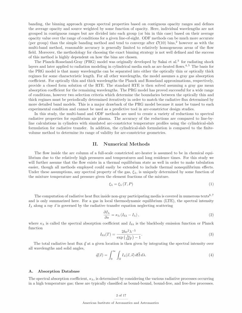
The total radiative heat flux is determined via Eq. 4 where the limits of integration over λ range over theentire set of positive real values. In practice however, the spectral range is finite. For this study, the wave-length range was chosen in order to capture all important contributions of emission (κλIbλ) and absorption(κλIλ). Wien’s displacement law provides the wavelength where the blackbody emission is maximized for agiven temperature.

argmaxnλT

Ibλ = 2898 μmK (5)

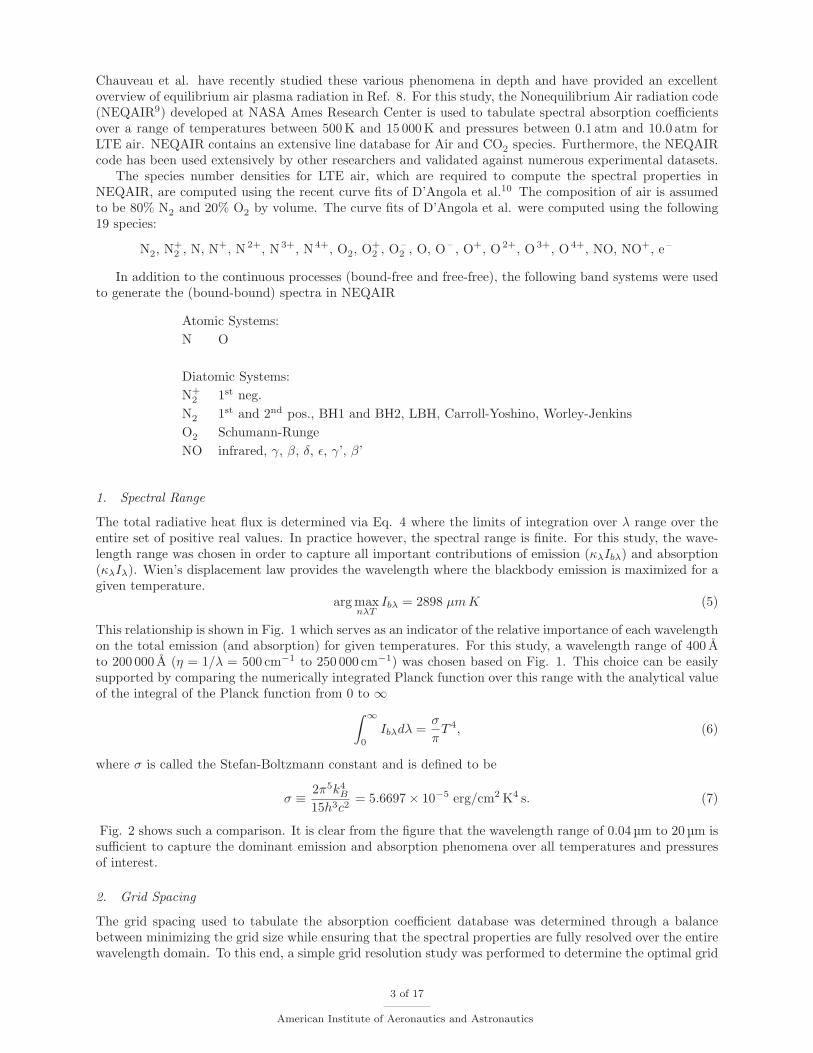
This relationship is shown in Fig. 1 which serves as an indicator of the relative importance of each wavelengthon the total emission (and absorption) for given temperatures. For this study, a wavelength range of 400 Ato 200 000 A (η = 1/λ = 500 cm−1 to 250 000 cm−1) was chosen based on Fig. 1. This choice can be easilysupported by comparing the numerically integrated Planck function over this range with the analytical valueof the integral of the Planck function from 0 to ∞∫ ∞

0

Ibλdλ =σ

πT 4, (6)

where σ is called the Stefan-Boltzmann constant and is defined to be

σ ≡ 2π5k4B15h3c2

= 5.6697× 10−5 erg/cm2 K4 s. (7)

Fig. 2 shows such a comparison. It is clear from the figure that the wavelength range of 0.04 μm to 20μm issufficient to capture the dominant emission and absorption phenomena over all temperatures and pressuresof interest.

2. Grid Spacing

The grid spacing used to tabulate the absorption coefficient database was determined through a balancebetween minimizing the grid size while ensuring that the spectral properties are fully resolved over the entirewavelength domain. To this end, a simple grid resolution study was performed to determine the optimal grid

3 of 17


10000

1e+06

1e+08

1e+10

1e+12

1e+14

1e+16

1e+18

100 1000 10000 100000 1e+06

Bla

mbd

a [W

/cm

3 ]

lambda [A]

Wien’s Displacement Law

300 K

1,000 K

5,000 K

10,000 K

15,000 K

Wien’s Distribution

Figure 1: Wien’s distribution showing affectivewavelength range for temperatures between 300Kand 15 000K.

0.001

0.01

0.1

1

10

100

1000

10000

100000

1e+06

0 2000 4000 6000 8000 10000 12000 14000 16000

Inte

gral

of P

lanc

k’s

Func

tion

[W/c

m2 -s

r]

Temperature [K]

Validation of Planck Function Integral (10 bins)

sigma/pi*T4

P = 1 atmP = 10 atm

Figure 2: Comparison of the integrated Planck func-tion with limits of integration from 0.04 μm to 20 μmand the theoretical curve for 0 to ∞.

spacing necessary to meet both criteria. It was determined that the following grid ranges and spacings inTable 1 provide fully resolved κλ while minimizing erroneous wavelength points. The total size of the entiregrid is 1,051,755 wavelengths.

Table 1: Wavelengthgth grid used in neqair.inp.

λ1 [A] λ2 [A] Δλ [A] Points

400 2,000 0.04 40001

2,000 6,350 0.10 43501

6,350 200,000 0.20 968253

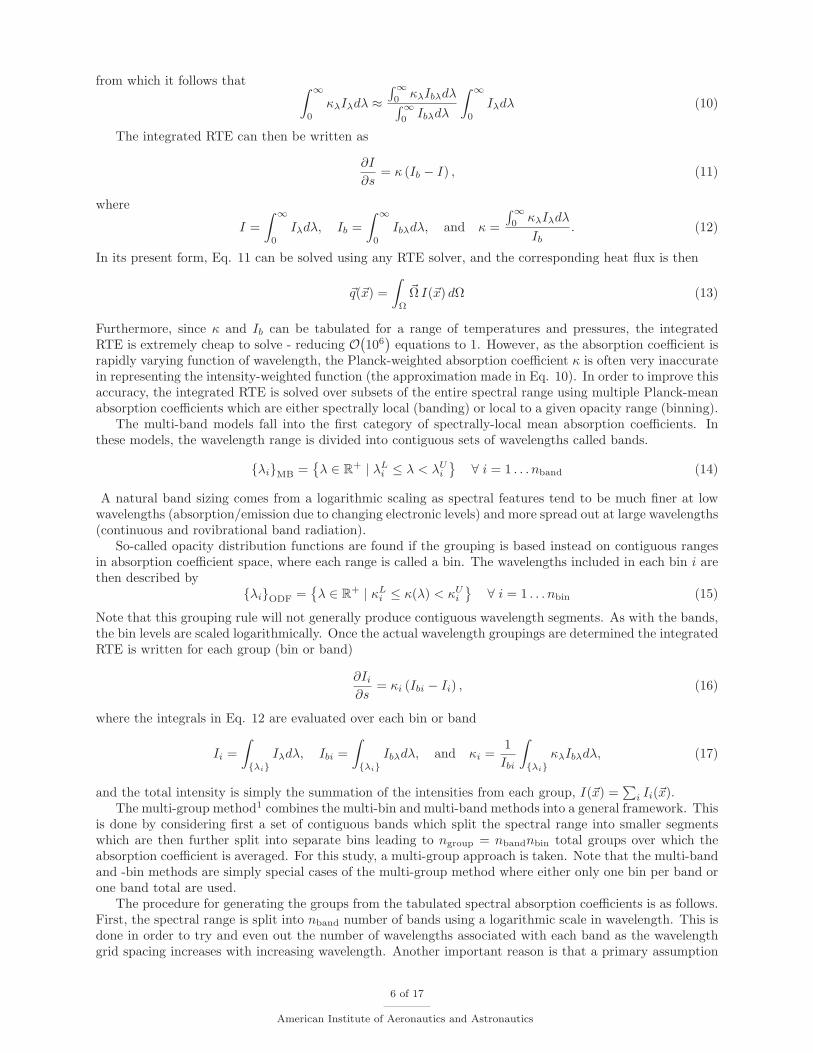
The resulting absorption coefficient spectrums for five different temperatures at 1 atm for LTE air ascomputed by NEQAIR are presented in Fig. 3. From the figure, it is clear that the spectral absorptioncoefficient varies wildly with wavelength and temperature due to the highly non gray nature of the absorb-ing/emitting gas and the changing chemical composition due to the LTE air formulation. Solving the RTEin Eq. 2 requires integrating over each spectral wavelength, line of sight, and solid angle. Performing thefull integration in this way is called a line-by-line calculation and represents the most accurate method forcomputing the radiative transfer in a non gray medium. For 3-dimensional geometries, this can pose animpractical computational task, especially when it is desired to couple the radiation field to the flow fieldgoverned by the Navier-Stokes equations. (Note: the strong, isolated downward-pointing spikes in Fig. 3(a), (b), and (c) are artifacts of the wavelength domain decomposition and are not physical.)

B. Multi-band Model and Opacity Distribution Functions

In essence, the multi-band model and the opacity distribution function model (multi-bin) are similar methodsin that they both attempt to reduce the dimensionality of the wavelength space by grouping individualwavelength’s together and defining an average absorption coefficient (opacity) and emissivity for each group.The primary difference lies in how the groups are formed. This common ground allows a succinct developmentof both methods starting with an identical formulation but diverging in the formation of the groups.

The radiative heat flux is computed using Eq. 4. Since the direction-cosine of the ray �s is not a functionin wavelength (or any spectral quantity), the integral over wavelength in Eq. 4 may be moved inside theradiative transfer equation, Eq. 2.

∂

∂s

∫ ∞

0

Iλdλ =

∫ ∞

0

κλIbλdλ−∫ ∞

0

κλIλdλ (8)

4 of 17


10-20

10-15

10-10

10-5

100

105

0 25000 50000 75000 100000 125000 150000

Abs

orpt

ion

Coe

ffici

ent [

cm-1

]

Wavenumber [cm-1]

(a) 5000K

10-8

10-6

10-4

10-2

100

102

104

106

0 25000 50000 75000 100000 125000 150000

Abs

orpt

ion

Coe

ffici

ent [

cm-1

]

Wavenumber [cm-1]

(b) 8000K

10-6

10-5

10-4

10-3

10-2

10-1

100

101

102

103

104

105

0 25000 50000 75000 100000 125000 150000

Abs

orpt

ion

Coe

ffici

ent [

cm-1

]

Wavenumber [cm-1]

(c) 10 000K

10-5

10-4

10-3

10-2

10-1

100

101

102

103

104

105

0 25000 50000 75000 100000 125000 150000

Abs

orpt

ion

Coe

ffici

ent [

cm-1

]

Wavenumber [cm-1]

(d) 12 000K

10-4

10-3

10-2

10-1

100

101

102

103

104

0 25000 50000 75000 100000 125000 150000

Abs

orpt

ion

Coe

ffici

ent [

cm-1

]

Wavenumber [cm-1]

(e) 15 000K

Figure 3: Absorption coefficient spectra for an LTE air plasma at 1 atm and multiple temperatures.

Note that the above equation does not make any assumptions or approximations and is still completely validin a mathematical sense. However, the right-hand term of the right side of Eq. 8 is not closed and cannotbe determined. In order to close the equation the following approximation is made.∫∞

0κλIλdλ∫∞

0Iλdλ

≈∫∞0

κλIbλdλ∫∞0

Ibλdλ(9)

5 of 17


from which it follows that ∫ ∞

0

κλIλdλ ≈∫∞0

κλIbλdλ∫∞0

Ibλdλ

∫ ∞

0

Iλdλ (10)

The integrated RTE can then be written as

∂I

∂s= κ (Ib − I) , (11)

where

I =

∫ ∞

0

Iλdλ, Ib =

∫ ∞

0

Ibλdλ, and κ =

∫∞0

κλIλdλ

Ib. (12)

In its present form, Eq. 11 can be solved using any RTE solver, and the corresponding heat flux is then

�q(�x) =

∫Ω

�Ω I(�x) dΩ (13)

Furthermore, since κ and Ib can be tabulated for a range of temperatures and pressures, the integratedRTE is extremely cheap to solve - reducing O(

106)equations to 1. However, as the absorption coefficient is

rapidly varying function of wavelength, the Planck-weighted absorption coefficient κ is often very inaccuratein representing the intensity-weighted function (the approximation made in Eq. 10). In order to improve thisaccuracy, the integrated RTE is solved over subsets of the entire spectral range using multiple Planck-meanabsorption coefficients which are either spectrally local (banding) or local to a given opacity range (binning).

The multi-band models fall into the first category of spectrally-local mean absorption coefficients. Inthese models, the wavelength range is divided into contiguous sets of wavelengths called bands.

{λi}MB ={λ ∈ R

+ | λLi ≤ λ < λU

i

} ∀ i = 1 . . . nband (14)

A natural band sizing comes from a logarithmic scaling as spectral features tend to be much finer at lowwavelengths (absorption/emission due to changing electronic levels) and more spread out at large wavelengths(continuous and rovibrational band radiation).

So-called opacity distribution functions are found if the grouping is based instead on contiguous rangesin absorption coefficient space, where each range is called a bin. The wavelengths included in each bin i arethen described by

{λi}ODF ={λ ∈ R

+ | κLi ≤ κ(λ) < κU

i

} ∀ i = 1 . . . nbin (15)

Note that this grouping rule will not generally produce contiguous wavelength segments. As with the bands,the bin levels are scaled logarithmically. Once the actual wavelength groupings are determined the integratedRTE is written for each group (bin or band)

∂Ii∂s

= κi (Ibi − Ii) , (16)

where the integrals in Eq. 12 are evaluated over each bin or band

Ii =

∫{λi}

Iλdλ, Ibi =

∫{λi}

Ibλdλ, and κi =1

Ibi

∫{λi}

κλIbλdλ, (17)

and the total intensity is simply the summation of the intensities from each group, I(�x) =∑

i Ii(�x).The multi-group method1 combines the multi-bin and multi-band methods into a general framework. This

is done by considering first a set of contiguous bands which split the spectral range into smaller segmentswhich are then further split into separate bins leading to ngroup = nbandnbin total groups over which theabsorption coefficient is averaged. For this study, a multi-group approach is taken. Note that the multi-bandand -bin methods are simply special cases of the multi-group method where either only one bin per band orone band total are used.

The procedure for generating the groups from the tabulated spectral absorption coefficients is as follows.First, the spectral range is split into nband number of bands using a logarithmic scale in wavelength. This isdone in order to try and even out the number of wavelengths associated with each band as the wavelengthgrid spacing increases with increasing wavelength. Another important reason is that a primary assumption

6 of 17


0.1

1

10

100

1000

300 350 400 450 500

Abs

orpt

ion

Coe

ffici

ent [

1/cm

]

Wavelength [nm]

Bin 1 Bin 2 Bin 3 Bin 4

(a) Unordered absorption coefficient spectrum.

0.1

1

10

100

1000

0 5000 10000 15000 20000

Abs

orpt

ion

Coe

ffici

ent [

1/cm

]

Index

Bin 1 Bin 2 Bin 3 Bin 4

(b) Ordered absorption coefficient spectrum.

Figure 4: Example showing how the binning procedure works with 4 bins in the 300 nm to 500 nm range forequilibrium Air at 10 000K and 1 atm.

of the binned RTE methodology is that the Planck function is considered constant over each group. FromFig. 1 it is clear that Ibλ varies exponentially at lower wavelengths. In addition to the logarithmic scaling,an additional constraint is placed on the bands. It was found during the course of testing that since above100 μm, κλ is a smooth function of λ, it was beneficial to force the last band to cover the 100μm to 200μmrange. This constraint improves accuracy by allowing the remaining bands to cover a smaller spectral range.

After the wavelengths are split into bands, each band is then subdivided into nbin bins. Several strategiesfor determining the opacity ranges which determine the bins in each band were tested. If a constant orlogarithmic spacing was used, it is was found that not all bins were guaranteed to contain at least a singlewavelength. In addition, it was likely that one bin would contain over 90% of the wavelengths in the bandand thus the other bins would suffer from a statistical point of view. In light of these issues, another methodwas adopted in which the spectral absorption coefficients were first ordered in each band and the bin rangeswere determined by assigning equal numbers of wavelengths to each bin. This process is shown graphicallyin Fig. 4.

After assigning each wavelength to a group, the mean absorption coefficient and integrated Planck func-tion as defined in Eq. 17 were computed for each group and tabulated versus temperature and pressure toform a reduced spectral model. One important observation about the integration method should be noted.Originally, the authors attempted to use the trapezoidal rule for computing the integrals in Eq. 17, however,as can be easily verified, the trapezoidal rule is not consistent with the original RTE. In other words, whenthe number of groups approaches the number of wavelengths, the accuracy of the “reduced” model shouldconverge to LBL, however this is not the case when trapezoidal rule is used because cross-multiplicationterms are introduced between spectral values. These inconsistencies actually increase the error of a reduc-tion substantially as the number of groups increase. Therefore, the rectangular rule was used instead toperform the numerical integration which is consistent with LBL calculations.

C. Cylindrical Slab Formulation

The equations for radiative heat flux in a cylindrical “slab” are derived in the paper by Kesten et. al.11 Tocompute the radiation intensity in the radial direction at a point O (see Fig. 5), they analytically integratethe equation representing the change in intensity along a light beam, Eq. 2, starting at a point A, on thecylinder wall, passing through point O.

After a series of coordinate transformation and analytical integration over angles, they write,

ql(r) = 4∫ π/2

0

[Il|RD3

{∫ r cos γ

0κnu(y

′′)dy′′ +∫√R2−r2 sin2 γ

0κnu(y

′′)dy′′}

+∫√R−r2 sin2 γ

0D2

{∫ r cos γ

0κnu(y

′′)dy′′ +∫ y′

0κnu(y

′′)dy′′}ηl(y

′)dy′

7 of 17


α�

��

��

��

��

Figure 5: Ray path (AOB) in cylindrical geometry. The coordinates (s and x) and angles are shown on thefigure.

8 of 17


0<γ<π/2�

��

��

��

��

��

π/2<γ<π�

��

��

��

γ �

�� γ

γ �

Figure 6: Ray paths during integration in γ. Two rays are shown, one corresponding to A’OB’ (0 ≤ γ′ ≤ π/2),the other corresponding to A”OB” with γ′′ = π − γ′.

+∫ r cos γ

0D2

{∫ r cos γ

y′ κ(y′′)dy′′}ηl(y

′)dy′]cos γdγ

−4∫ π/2

0

[Il|RD3

(∫√R2−r2 sin2 γ

r cos γκl(y

′)dy′)

+∫√R2−r2 sin2 γ

r cos γD2

(∫ y′′

r cos γκl(y

′)dy′)ηl(y

′′)dy′′]cos γdγ

(18)

where Il|R is the radiative intensity at the wall and Dn is the exponential integral function,

Dn(x) =

∫ 1

0

μn−1√1− μ2

exp(−x/μ)dμ

Nicolet et al.12 developed a numerical algorithm to solve Eq. 18. They start by adopting an approxima-tion to Dn using exponential fits of the form,13

Dn(x).= an exp(−bnx), (19)

and substitute the above in Eq. 18. They chose a best fit to D3, and have set,

b2 = b3 = 5/4

a2 = a3 = π/4

The cylinder is then discretized into N mesh points. They derived the final approximation to Eq. 18using logarithmic quadrature rules to obtain,

ql,i = (q+l,i − q−l,i)

9 of 17


where,

q±l,i = 4

N∑j=2

G±i,j +G±

i,j−1

2

(rjri

− rj−1

ri

)(20)

Nicolet et al.12 used a band approximation where they have set Il|R, the radiative energy flux at thewall, to be the integral of the emissivity in a band [ll, ll+1], determined by,

Il|R = σT 4(f(ξl)− f(ξl+1))

where f(ξl) is the fractional function,

f(ξl) =

∫ ∞

ξl

ξ3

exp(ξ)− 1dξ

and ξl = hc/(λlkBT ).The expressions for G−

i,j and G+i,j in Eq. 20, are Eq. (A-21) and (A-22), given in Nicolet et al.12

D. Finite Volume Radiative Transfer

For verification of the cylindrical slab results, the radiative transfer problem was also solved by means of a3-d finite-volume method using the same spectral absorption coefficients and emission function. We writethe radiative transfer equation, Eq. 2, in three-dimensional form as

Ω · ∇Iλ(x,Ω) = κλ(x) (Ibλ(x)− Iλ(x,Ω)) , (21)

where Ω is the direction of propagation and x is the spatial position. The distance variable s in Eq. 2 ismeasured along the vector Ω. Upon integration of Eq. 21 over a computational cell we obtain∫

cell surface

Iλ(x,Ω)Ω · dS =

∫cell volume

κλ(x) (Ibλ(x)− Iλ(x,Ω)) dV. (22)

Discretizing Eq. 22 by approximating the volume integral with the value of the integrand at the cell centertimes the volume and approximating the surface integral by a summation over the faces of face-centeredvalues times the corresponding areas, one obtains∑

faces k

Iλ(xk,Ω)Ω ·ΔSk = κλ(xc) (Ibλ(xc)− Iλ(xc,Ω))V, (23)

where xc is the position of the cell center, xk is the position of the center of face k, V is the cell volume,and ΔSk is the outward-pointing surface area vector of face k of the cell. Splitting the surface summationinto incoming and outgoing parts and using cell-center values for the outgoing facial intensities in each cell,one gets the standard finite-volume method for radiative transfer:7

Iλ(xc,Ω) =κλ(xc)Ibλ(xc)V +

∑k,Ω·ΔSk<0 Iλ(xk,Ω) |Ω ·ΔSk|

κλ(xc)V +∑

k,Ω·ΔSk>0 Ω ·ΔSk. (24)

While this classic formula, Eq. 24, is an adequate approximation for many applications, we used a similarbut more accurate formulation.14 This method allows for significant variation in Iλ(x,Ω) across a cell. Theoutgoing intensity at each outgoing face is given in this method by

Iλ(xo,Ω) =

∑k,Ω·ΔSk<0 Iλ(xk,Ω) |Ω ·ΔSk|∑

k,Ω·ΔSk>0 Ω ·ΔSke−κλ(xc)d + (1− e−κλ(xc)d)Ibλ(xc), (25)

where xo is the position of an outgoing face, and

d =V∑

k,Ω·ΔSk>0 Ω ·ΔSk(26)

is the average value of the distance across the cell from the incoming to the outgoing faces in direction Ω.

10 of 17


The value of Iλ(xo,Ω) is computed using Eq. 25 for a set of Ω vectors, the so-called discrete ordinatemethod.7 This set is chosen to produce an accurate quadrature over the 4π direction space for computingthe divergence of the radiative heat flux, ∇·qλ . The average radiative heat flux in a cell is thereby computedvia

1

V

∫cell volume

∇ · qλ dV =1

V

∫cell surface

qλ · dS (27)

≈ 1

V

∫4π

∑faces k

Iλ(xk,Ω)Ω ·ΔSk dΩ (28)

≈ 1

V

∑i

∑faces k

Iλ(xk,Ωi)Ωi ·ΔSk ΔΩi (29)

where the weights ΔΩi are given by the chosen quadrature formula. In this work all angular quadratureswere done with the S4 set of discrete ordinates, which uses 24 directions Ωi.

III. Results and Discussion

A. Reductions

High pressure arc-columns typically have a hot core near the upstream region which expands and coolsdownstream. The radial temperature profile inside a column resembles a gaussian temperature distributionwith a peak temperature in the center and a fixed wall temperature at the radius of the column. Thetemperature distribution of Eq. 30 has been created in order to simulate such profiles at different downstreamcross-sections.

T (r) = (Twall − Tmax)

[exp

(−(r/R)2/2σ2)− 1

exp (−1/2σ2)− 1

]+ Tmax (30)

The temperature distribution is parameterized based on the maximum and wall temperatures, Tmax and Twall,the radius of the column, R, and a stretching factor, σ, which corresponds to the variance of the gaussianprofile. Three temperature profiles have been chosen to test the performance of the spectral reductions usingEq. 30. The values of Tmax, Twall, R, and σ are given in Table 2 and the actual temperature profiles areplotted graphically in Fig. 7.

Table 2: Parameters corresponding to model temperature distribution used to test the accuracy of variousmodel reductions (see Eq. 30).

Name Tmax Twall R (cm) σ

G08 8,000 1,000 1.5 1000

G10 10,000 1,000 1.5 1

G12 12,000 1,000 1.5 0.5

Several reductions were computed using the methodology described in Section B. A variety of band andbin combinations were chosen in order to study the overall effectiveness of the methodology in accuratelyreducing the full spectrum of absorption coefficients to a manageable number. Each reduction was comparedto LBL calculations using the cylindrical-slab method for the three temperature distributions detailed inTable 2. The accuracy of each reduction is assessed based on two criteria. The first criteria, ε∇·�q, is basedon the relative, maximum percent difference of ∇ · �q(r) as compared to the LBL calculation along the entireradial distance in the column.

ε∇·�q =maxr (∇ · �qLBL(r)−∇ · �q(r))

maxr |∇ · �qLBL(r)| × 100% (31)

Note that defining the error in the radiative source term in this way does not lead to large relative errorswhen ∇ · �q(r) is nearly zero. Instead, this criterion gives a sense of the maximum error with respect to the

11 of 17


0

2000

4000

6000

8000

10000

12000

14000

0 0.2 0.4 0.6 0.8 1 1.2 1.4 1.6

Tem

pera

ture

[K]

Radial Location [cm]

G12G10G08

Figure 7: Gaussian temperature profiles from Table 2.

overall order of magnitude of the peak heating within the column. The second criteria, εqr,wall, is the relative

error in the radiative heat flux at the wall as compared to LBL.

εqr,wall=

qr,LBL(R)− qr(R)

qr,LBL(R)× 100% (32)

Table 3 summarizes the 28 different reductions computed and their accuracies as compared to LBL basedon the above two criteria. The table is ordered by increasing bands and then increasing bins to show the clearrelationship the number of bands has on the overall accuracy of the reduction. Regardless of the number ofbins used in the reduction, an error of less than 10% for all temperature profiles cannot be obtained withless than 1000 bands. It is also important to note that in general, it appears that the radial heat flux at thewall is easier to accurately predict than the divergence of the heat flux within the column, however for all ofthe pure binning cases (1-5), the opposite trend is observed.

Fig. 8 presents the error criterion of Table 3 in a graphical way making it easier to visualize the overalltrends. It is clear from the figure that indeed the wall radiative heat flux is better predicted by the reducedmodels as compared to the divergence of the flux in the column. The bulk of the εqr,wall

values are centeredaround 10% where as the ε∇·�q values trend closer to 100%. Fig. 8 also highlights another important (thoughexpected) result. The colors in the figure represent which temperature profile in Table 2 the errors belongto. It is therefore clear to see that in nearly all cases, the lower the peak heating is, the better each reducedmodel can predict the radiative heating within the cylinder. This suggests that a practical RTE solver couldselect from a range of reduced models depending on the core temperature of the arc-column, enabling acomputational speedup in the downstream regions where the temperatures are more uniform.

Fig. 9 shows the actual qr and ∇ · �q profiles for the LBL and five reductions in Table 3 which have thelowest overall errors. The heat flux within the column first peaks to a maximum due to the hot core at thecenter before the absorption in the colder regions towards the wall tends to equilibrate the radiative flux fromboth directions. The radiative flux at the wall is much lower than the peak location, owing to the absorptionin the wall region. Interestingly, the errors in the peak heating region due to the various reductions shownin Fig. 9a have little affect on the final radiative flux reaching the wall, suggesting that the cold region isoptically thick.

In addition, it is clear that small differences in the core temperature result in very large differences inpeak heating as can be seen by comparing the ∇·�q profiles for each temperature distribution in Fig. 9b. Thisis most likely due to the fact that at 10 000K, atomic nitrogen is at its peak concentration before ionizationbegins for equilibrium air at 1 atm. Above 10 000K, the concentrations of N+ and e – begin to become

12 of 17


Table 3: Summary of the errors, ε∇·�q (Eq. 31) and εqr,wall(Eq. 32), of each reduction tested on the gaussian

temperature profiles listed in Table 2.

G08 G10 G12

No. Type nband nbin ngroup ε∇·�q εqr,wallε∇·�q εqr,wall

ε∇·�q εqr,wall

1. bins 1 10 10 -26.0 -149.7 -84.6 -122.1 -121.8 -179.7

2. bins 1 20 20 -26.0 -147.9 -82.2 -119.5 -118.5 -174.7

3. bins 1 50 50 -25.9 -147.0 -79.4 -117.2 -116.4 -171.6

4. bins 1 100 100 -25.9 -146.5 -78.9 -116.7 -116.2 -170.9

5. bins 1 500 500 -25.9 -145.4 -76.4 -114.8 -114.2 -167.9

6. multi-group 4 50 200 -9.9 -9.4 -81.4 -8.6 -113.5 -12.6

7. multi-group 5 5 25 -47.5 -41.6 -227.6 -92.4 -170.7 -115.5

8. multi-group 5 10 50 -43.2 -13.8 -207.6 -21.4 -153.4 -26.2

9. multi-group 5 20 100 -38.3 -8.5 -172.0 -8.4 -129.7 -9.2

10. multi-group 8 25 200 -8.3 -4.4 -72.8 -5.3 -94.2 -6.0

11. bands 10 1 10 -174.5 -102.4 -733.7 -397.1 -475.7 -482.5

12. multi-group 10 5 50 -122.2 -10.8 -322.8 -16.1 -212.5 -25.5

13. multi-group 10 10 100 -77.0 -7.9 -129.2 -9.6 -100.0 -16.2

14. multi-group 10 20 200 -32.6 -7.0 -50.1 -8.3 -57.5 -13.0

15. multi-group 10 50 500 -3.9 -6.6 -32.2 -6.8 -51.3 -9.2

16. multi-group 20 5 100 -44.9 -6.0 -175.4 -8.6 -134.4 -15.2

17. multi-group 20 10 200 -27.8 -4.7 -99.2 -6.4 -85.4 -11.0

18. multi-group 20 25 500 -12.2 -4.3 -41.6 -4.2 -55.8 -6.6

19. multi-group 25 8 200 -23.6 -3.6 -82.6 -6.2 -69.2 -11.3

20. multi-group 25 20 500 -12.0 -3.5 -39.0 -4.8 -47.9 -7.8

21. multi-group 50 4 200 -26.7 -2.6 -79.3 -4.7 -59.1 -8.2

22. multi-group 50 10 500 -12.4 -2.9 -31.6 -5.0 -34.9 -7.8

23. bands 100 1 100 -50.7 2.6 -161.7 -15.0 -136.0 -23.4

24. multi-group 100 2 200 -26.5 -1.2 -75.2 -9.9 -58.2 -14.8

25. multi-group 100 5 500 -10.5 -2.9 -27.4 -7.3 -27.8 -10.1

26. bands 500 1 500 -16.5 4.6 -40.6 -7.0 -38.4 -12.9

27. bands 1000 1 1000 -5.8 4.8 -7.3 -0.8 -3.9 -1.9

28. bands 10000 1 10000 4.9 4.1 -2.2 2.0 1.1 3.5

substantial which increase the radiant power due to bound-free and free-free transitions. Thus, the peakheating at 12 000K is about −16 kW/cm3 while at 10 000K and 8000K the peak heating is only −2 kW/cm3

and −0.5 kW/cm3 respectively. This observation underlines the importance of accurately predicting the gascomposition in the column which can be highly dependent on the radiative-flow coupling.

Finally, we consider the poor performance of the pure binning reductions (reductions 1-5 in Table 3).Surprisingly, the performance of the reductions is barely affected by the number of bins used. For example,the error in the radiative flux at the wall for the G12 temperature profile changes from 179.7% with just 10bins to only 167.9% with 500 bins. In contrast, the pure banding yields for the same error criteria 482.5%error with only 10 bands but just 12.9% with 500 bands.

Fig. 10 shows the qr and ∇ · �q profiles for each temperature distribution using each of the pure binningreductions as compared to the LBL calculations. As hinted at by the errors listed in Table 3, the purebinning profiles are nearly identical regardless of the number of bins used. Several authors have previouslynoted that the assumption made in Eq. 16 is that each group of wavelengths (either bins or bands or mixed)either spans a spectral region in which the Planck function is nearly constant, or the spectral absorption

13 of 17


0.1

1

10

100

1000

10 100 1000 10000

Per

cent

Err

or in

div

(q)

[%]

Number of Groups

(a) ε∇·�q

0.1

1

10

100

1000

10 100 1000 10000

Per

cent

Err

or in

qw

all [

%]

Number of Groups

(b) εqr,wall

Figure 8: Results of Table 3 shown graphically. Symbols represent type of reduction (�, pure binning; �,pure banding; , mixed). Colors represent the temperature distribution (red, G12; green, G10; blue, G08).

0

200

400

600

800

1000

1200

1400

1600

0 0.2 0.4 0.6 0.8 1 1.2 1.4 1.6

q r [W

/cm

2 ]


G12

G10

G08

LBL500 Bands

1,000 Bands10,000 Bands

50 Bands, 10 Bins100 Bands, 5 Bins

(a) qr

-2000

0

2000

4000

6000

8000

10000

12000

14000

16000

18000

20000

22000

24000

0 0.2 0.4 0.6 0.8 1 1.2 1.4 1.6

div(

q) [W

/cm

3 ]


G12

G10

G08

LBL500 Bands

1,000 Bands10,000 Bands

50 Bands, 10 Bins100 Bands, 5 Bins

-1000

-500

0

500

1000

1500

2000

2500

3000

0 0.2 0.4 0.6 0.8 1 1.2 1.4 1.6

(b) ∇ · �q

Figure 9: Comparison of LBL and reduced model calculations of the radiative heat flux and its divergencefor the temperature distributions shown in Fig. 7. Only the five reductions with the smallest errors as givenin Table 3 are shown.

coefficient can be treated as randomly distributed such that the errors associated with the Planck-weightedmean absorption coefficient are small. If either assumption is not met, then the errors in the reduction will belarge. Therefore, the poor performance of the pure binning reductions as shown in Fig. 10 can be attributedto the fact that the bins may span the entire wavelength spectrum, in which case the Planck function canrange over many orders of magnitude. This is further substantiated by the observation that using a fewbands to divide the wavelength spectrum into smaller regions can dramatically increase the accuracy of thereductions. For instance, using 500 bins alone (reduction 5) yielded a εqr,wall

value of -167.9%, however if thetotal wavelength range is split into 10 subregions with 50 bins each (reduction 15), this error drops to -9.2%(note that the error in the divergence term is still over 51% for this case).

B. Cylindrical-Slab vs. Finite-Volume

In the following section, a comparison is made between the cylindrical-slab formulation and the finite-volumeformulations detailed in previous sections. This is done in order to both verify the correctness of the thecylindrical-slab formulation as well as to determine when it is valid to use this method for arc-jet geometries.

14 of 17


0

500

1000

1500

2000

2500

0 0.2 0.4 0.6 0.8 1 1.2 1.4 1.6

q r [W

/cm

2 ]


G12

G10

G08

LBL10 Bins20 Bins50 Bins

100 Bins500 Bins

(a) qr

-2000

2000

6000

10000

14000

18000

22000

26000

30000

34000

38000

0 0.2 0.4 0.6 0.8 1 1.2 1.4 1.6

div(

q) [W

/cm

3 ]


G12

G10

G08

LBL10 Bins20 Bins50 Bins

100 Bins500 Bins

-1000

0

1000

2000

3000

4000

0 0.2 0.4 0.6 0.8 1 1.2 1.4 1.6

(b) ∇ · �q

Figure 10: Comparison of LBL and pure binning calculations of the radiative heat flux and its divergencefor the temperature distributions shown in Fig. 7.

To begin, Eq. 30 is rewritten in two dimensions by linearly interpolating from a constant wall temperature,Twall, at z = 0 to a gaussian temperature profile with peak temperature, Tmax, at z = L.

T (ρ, ζ) = (1− ζ)Twall + ζ

{(Twall − Tmax)

[expα(ρ, ζ)− 1

expα(1, ζ)− 1

]+ Tmax

}, (33)

where

ρ =r

R, ζ =

z

L, α(ρ, ζ) =

−0.5ρ2

(ζσ1 + (1− ζ)σ2)2 . (34)

The benefit of such a parameterization is that it is nondimensionalized by the cylinder’s length and radius,thus radial temperature profiles at a particular non dimensional cross-section, ζ, remain unchanged whenthe length of the cylinder, L, is changed. As with the stretching factor σ in Eq. 30, the factors σ1 and σ2 inEq. 34 determine how stretched the gaussian profiles are at z = L and z = 0 respectively. For the remainderof this section, these values are taken to be σ1 = 0.2 and σ2 = 1.0. Fig. 11 shows the progression of radialtemperature profiles for these stretching factors in the non dimensional coordinates of Eq. 34.

The finite-volume method was used to compute the radiative flux and its divergence in a cylinder whosetemperature profile is constant in the angular direction and follows the temperature parameterization of Eq.33 in the radial and axial directions. The radius of the cylinder, R, was taken to be 3 cm and four separatelengths were chosen corresponding to L = 10R, 20R, 30R and 40R. The computational domain was split into300 radial cells, 300 axial cells, and 20 angular cells totaling 1.8 million cells to model the entire domain. Inorder to limit computational time, the 1000 band reduction (number 27 in Table 3) was used to representthe spectral properties of the gas.

Fig. 12 presents the radial heat flux and the divergence as a function of the radial location at the 0.5Lcross-section of the cylinders (averaged over each angular location) compared to the solution obtained for thesame temperature profile using the cylindrical-slab formation with the 1000 band reduction. As can be seenfrom the figure, as the L/R ratio increases, the cylindrical-slab formulation becomes closer to reproducingthe exact integration for the radiative heat flux in the radial direction. This could be expected but itis far from guaranteed as the assumptions made by the cylindrical-slab formulation are 1) the cylinder isinfinitely long, and 2) the spectral properties vary only in the radial direction. The first assumption is clearlyapproached with an increasing L/R ratio, however the second assumption is less obvious. However, from theabove results, it is clear that allowing small deviations in the radiative properties in the axial direction is asufficient condition for the applicability of the cylindrical-slab formulation.

Fig. 12 shows that for the particular temperature parameterization given, the cylindrical-slab formulationis accurate for cylindrical geometries with L/R � 30. For comparison, Nicolet et al.12 collected sizeinformation of various constricted arc heaters in use in 1975. The L/R values for these constrictors rangedfrom about 14 to over 162 where all but one had a minimum L/R of 30. The Interactive Heating Facility

15 of 17


Twall

Tmax

0 0.2 0.4 0.6 0.8 1

Tem

pera

ture

ρ

ζ = 1.0

ζ = 0.8

ζ = 0.6

ζ = 0.4

ζ = 0.2

ζ = 0.0

σ1 = 0.2

σ2 = 1.0

Figure 11: Radial temperature profiles given by Eq. 33 at several cross-sections along the cylinder forstretching factors σ1 = 0.2 and σ2 = 1.0.

0

20

40

60

80

100

120

140

160

0 0.5 1 1.5 2 2.5 3

q [W

/cm

2 ]


FV, L = 10RFV, L = 20RFV, L = 30RFV, L = 40R

Cyl. Slab

(a) qr

-100

0

100

200

300

400

500

0 0.5 1 1.5 2 2.5 3

div(

q) [W

/cm

3 ]


FV, L = 10RFV, L = 20RFV, L = 30RFV, L = 40R

Cyl. Slab

(b) ∇ · �q

Figure 12: Comparison of the radial heat flux and the divergence of the heat flux for finite-volume calculationsperformed with varying the length of the cylinder versus a cylindrical slab formulation.

(IHF) and the Aerodynamic Heating Facility (AHF) at NASA Ames Research Center operate today at L/Rratios of 97.3 and 79.6 respectively.

In terms of performance, the cylindrical-slab formulation was two orders of magnitude faster than thefinite-volume solver after taking into account that the cylindrical-slab code must be used at every axialcross-section. In addition, because each cross-section is treated as independent, the cylindrical-slab lendsitself to a higher degree of parallelization. This increase in performance along with a complete reduction inspectral properties makes fully coupled flow/radiation calculations possible for arc-constrictor simulationswhile maintaining a high level of accuracy.

16 of 17


IV. Concluding Remarks

Full LBL calculations of radiative transfer for real problems is in general computationally impracticalwith todays computational facilities. This is further compounded when coupling the radiative source termswith the energy conservation equation for fluid dynamics simulations. For cylindrical geometries, the aboveresults show that the cylindrical-slab formulation can reach the same accuracy as performing the full spatialintegration when the cylinder is long enough. One important application of this methodology is modelingthe radiative transfer occurring in high pressure arc-constrictors which greatly impacts the flow inside theconstrictor. The cylindrical-slab formulation provides a considerable increase in performance over the finite-volume method while retaining reasonable accuracy.

The computational performance can be further improved when a reduced radiation model is used. It wasshown in the above that a 1000 band reduction is sufficient to completely model equilibrium air radiation overa wide temperature and pressure range. Since line-by-line calculations are completely decoupled betweeneach wavelength, this reduction corresponds to another three orders of magnitude reduction from line-by-linecalculations.

The combined reduced model and cylindrical-slab formulation allow fully coupled flow/radiation calcula-tions to be performed for equilibrium air in cylindrical geometries such as that present arc-constrictor flows.In addition, the proposed model reduction does not require any additional information in order to “tune”the model for a particular set of conditions. This gives the model a truly predictive capability and will allowthe it to be used in future arc-constrictor design studies.

V. Acknowledgements

The authors would like to thank Dr. Aaron Brandis and Dr. Dinesh Prabhu for many helpful discussionsabout the use of the NEQAIR program.

References

1Cullen, D. E. and Pomraning, G. C., “The Multiband Method in Radiative Transfer Calculations,” J. Quant. Spectrosc.Radiat. Transfer , Vol. 24, 1980, pp. 97–117.

2A. A. Wray, J.-F. R. and Prabhu, D., “Investigation of the opacity binning approach for solving the shock-generatedradiation of the Apollo AS-501 re-entry,” Center for Turbulence Research, Proceedings of the Summer Program.

3Sakai, T., Sawada, K., and Park, C., “Assessment of Planck-Rosseland-Gray Model for Radiating Shock Layer,” AIAA,, No. AIAA-97-2560, 1997.

4Sakai, T. and Sawada, K., “Application of Planck-Rosseland-Gray Model for High Enthalpy Arc Heaters,” AIAA, 1998.5Takahashi, Y., Kihara, H., and ichi Abe, K., “The effects of radiative heat transfer in arc-heated nonequilibrium flow

simulation,” J. Phys. B: Appl. Phys., Vol. 43, No. 185201, 2010.6Vincenti, W. G. and Kruger, C. H., Introduction to Physical Gas Dynamics, Krieger Pub Co, 1975.7Modest, M. F., Radiative Heat Transfer , Academic Press, 2nd ed., 2003.8Chauveau, S., Deron, C., Perrin, M.-Y., Riviere, P., and Soufiani, A., “Radiative transfer in LTE air plasmas for

temperatures up to 15,000 K,” Journal of Quantitative Spectroscopy & Radiative Transfer , Vol. 77, 2003, pp. 113–130.9Whiting, E. E., Park, C., Arnold, J. O., and Paterson, J. A., “NEQAIR96, Nonequilibrium and Equilibrium Radiative

Transport and Spectra Program: User’s Manual,” Reference Publication 1389, NASA, 1996.10D’Angola, A., Colonna, G., Gorse, C., and Capitelli, M., “Thermodynamic and transport properties in equilibrium air

plasmas in a wide pressure and temperature range,” Eur. Phys. J. D , Vol. 46, 2008, pp. 129–150.11Kesten, A. S., “Radiant Heat Flux Distribution in a Cylindrically-Symmetric Nonisothermal Gas with Temperature-

Dependent Absorption Coefficient,” J. Quantitative Spectroscopy and Radiative Transfer , Vol. 8, 1968, pp. 419–434.12Nicolet, W. E., Shepard, C. E., Clark, K. J., Balakrishnan, A., Kesselring, J. P., Suchsland, K. E., and Reese, J. J.,

“Analytical and Design Study for a High-Pressure, High-Enthalpy Constricted Arc Heater,” Tech. rep., Aerotherm, AEDC-TR-75-47, 1975.

13Wassel, A. T. and Edwards, D. K., “Molecular Gas Band Radiation in Cylinders,” J. Heat Transfer, Transactions ofASME , Vol. 96, 1974, pp. 21–26.

14Wray, A., “Improved Finite-Volume Method for Radiative Hydrodynamics,” Seventh International Conference on Com-putational Fluid Dynamics (ICCFD7).

17 of 17


Documents

Multi-Group Reductions of LTE Air Plasma Radiative ... · Multi-Group Reductions of LTE Air Plasma Radiative Transfer in Cylindrical Geometries ... line-by-line (LBL)accuracy