Glysson, G.D., 1987, Sediment Transport Curves: USGS Open-File

CONTENTS

Page

A b s t r a c t ..................................................... .... 1 I n t r o d u c t i o n . . . . . . . . . . . . . . . . . . . . . . . . . . . . . .e~~... . . . . . . . . . . . .e.. . . 1 Purpose and scope ..................................................... 2 Choice o f dependent and independent v a r i a b l e s ......................... 2 ............................................. Types o f t r a n s p o r t curves 4 Develop ing a sed iment - t ranspor t curve ................................. 4 V isua l f i t . . . . . . . . . . . . . . . . . . . . . . . . . . . . e~ .~~ . . . . . . . . . . . . . . . . . 15 ...................... L inea r r eg ress i on ................... .. .. ,. .. ... 15 ........................ Examples o f 1 i n e a r r eg ress i on method ... .. 17 Group average .. ........................................... 27 ................... Example o f group average method .. ....*.......a 31 Other problems assoc ia ted w i t h c o m p u t e r - f i t t e d curves ................. 35 P o t e n t i a l e r r o r s ................... ......ee.e.e ..................... 43 Summary . e . . . . . . ~ ~ . . e . . e ~ . . ~ e ~ O ~ e e e ~ ~ ~ e . . ~ . . . . . . . o e 46 .... References ............................................................ 46

ILLUSTRATIONS

F i gures 1.25 . Graphs showing

Comparison o f curves based on t h e same da ta b u t w i t h d i f f e r e n t independent v a r i a b l e s ............

Examples o f s i n g l e s t r a i g h t l i n e s no t adequate ly d e f i n i n g t h e r e l a t i o n between dependent and independent v a r i a b l e s ...........................

R e l a t i o n o f sediment d ischarge t o water d ischarge by storms f o r M i l l e r s Creek near P h y l l i s . Kentucky ........................................

Simultaneous sediment concen t ra t i on and water d ischarge peaks .................................

Sediment concen t ra t i on peak p reced ing t h e wate r d ischarge peak ..................................

Sediment concen t ra t i on peak l a g g i n g t h e water d i scha rge peak ....................... ... .... ... .

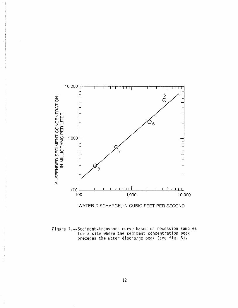
Sediment- t ranspor t cu rve based on recess ion samples f o r a s i t e where t h e sediment concent ra- ..... t i o n peak precedes t h e wate r d ischarge peak

R e l a t i o n o f suspended-sediment d ischarge t o water d ischarge a t M idd le Fork Eel R i v e r below B lack B u t t e R i ve r near Cove1 o. Cal i f o r n i a. 1963-68 wate r years ...............................*.ee * .

I n c o r r e c t r e l a t i o n o f sediment d ischarge t o water d ischarge by storms f o r M i l l e r s Creek near P h y l l i s . Kentucky ...............................

Instantaneous sed iment - t ranspor t curve f i t t e d by eye ..........................................

Sediment- t ranspor t cu rve f o r Eel R i v e r a t Sco t ia . C a l i f o r n i a . 1958-60 water years .................

ILLUSTRATIONS

Page

R e l a t i o n between sediment d ischarge and water discharge, us i ng l i n e a r r eg ress i on method, Yadkin R i v e r a t Yadkin Col lege, Nor th Caro l ina , ............................. 1969-73 water yea rs 25

Water d ischarge and sediment c o n c e n t r a t i o n hydrographs f o r Yadkin R i v e r a t Yadkin Col lege, Nor th Caro l ina , f o r February 23, 1971 ........... 26

R e l a t i o n between sediment d ischarge and water d ischarge f o r t h r e e peaks on Yadkin R i v e r a t Yadkin Col lege, Nor th C a r o l i n a .................. 28

Best es t imate o f t h e r e l a t i o n between sediment d ischarge and wate r d ischarge, Yadkin R i v e r near Yadkin Col lege, Nor th Caro l ina , 1969-73 water years ........................................... 29

R e l a t i o n between s t reamf low and suspended-sediment d ischarge, Feather R i v e r a t O r o v i l l e , C a l i f o r n i a , 1958 water yea r ........................v.*..... 30

Sediment- t ranspor t curves based on group averages method f o r Eel R i v e r a t Sco t ia , C a l i f o r n i a , 1958-60 water yea rs ............................. 34

D a i l y sediment d ischarge f o r a summer peak on a .................... smal l stream i n Pennsy lvan ia 36 Sediment- t ranspor t cu rve based on l o g - l i n e a r

r eg ress i on a n a l y s i s ........................,.... 37 Sediment- t ranspor t cu rve based on l og -quad ra t i c

r eg ress i on a n a l y s i s ............................. 38 Example o f two l o g - l i n e a r sed iment - t ranspor t

curves, one f o r r i s i n g and peak pe r i ods and one f o r recess ion pe r i ods ........................... 40

Example o f sediment -t ranspo r t cu rve based on t h e f l o w range sampled .......................... 41

Example o f problem t h a t may be encountered when sed iment - t ranspor t cu rve i s extended beyond t h e range o f f l ows sampled .......................... 42

Example o f d i f f e r e n t t ypes o f t r a n s p o r t curves f i t t e d t o t h e same da ta and v a r i a t i o n s i n R~ and s tandard e r r o r ( s ) .......................... 44

Example o f sed iment - t ranspor t cu rve ( f i g u r e 20) w i t h da ta f o r a d d i t i o n a l storms added ........... 45

TABLES

Page

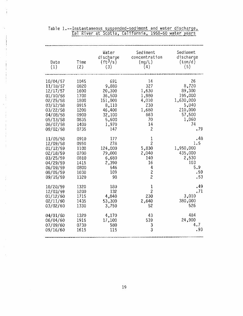
T a b l e 1. I n s t a n t a n e o u s suspended-sediment and w a t e r d i s c h a r g e , Eel R i v e r a t S c o t i a , C a l i f o r n i a , 1958-60 w a t e r y e a r s ..................................................... 19

2. Computat ion o f l o g a r i t h m i c l e a s t - s q u a r e s r e g r e s s i o n , Ee l R i v e r a t S c o t i a , C a l i f o r n i a , 1958-60 w a t e r

,, . y e a r s ..................................................... ZI 3. I n s t a n t a n e o u s suspended-sediment and w a t e r d i s c h a r g e ,

Yadkin R i v e r a t Yadkin Co l l ege , N o r t h C a r o l i n a , ....................................... 1969-73 w a t e r y e a r s 24 4. Computat ion o f s e d i m e n t - t r a n s p o r t r e l a t i o n u s i n g group

averages, Ee l R i v e r a t S c o t i a, Cal i f o r n i a, 1958-60 w a t e r y e a r s ............................................... 33 ............. 5. O r i g i n a l d a t a f i g u r e s 18-21 and 24 a r e based on 35

6. Es t ima ted sed iment d i s c h a r g e i n t o n s p e r day f o r i n d i c a t e d w a t e r d i s c h a r g e s ................................ 39

7. Comparison o f e r r o r s i n e s t i m a t i n g s t o r m sed iment l o a d s based on t h r e e s e d i m e n t - t r a n s p o r t cu rves ............ 43

e N

N

CO

CO

mm

m

r. N

W

OC

U-b

CQ

CO

CO

G

3O

b h0

LO

b

rn

OO

mN

N

om

0 0

-

mrn

rn

em

c3

00

0

-m

e

cnm

r.m

0

0.

0e

.a

D

O0

00

0

0

e

NW

00

00

0

+N

OM

OO

m

a

m

N

N

rr-C,

aJ #-a

a

L c c

UO

O

SEDIMENT-TRANSPORT CURVES

By G . Douglas Glysson

ABSTRACT

T h i s r e p o r t d e s c r i b e s t h e p rocess o f d e v e l o p i n g s e d i m e n t - t r a n s p o r t curves. It d i s c u s s e s t h e c h o i c e o f dependent and independen t v a r i a b l e s , p rocedures f o r d e v e l o p i n g a t r a n s p o r t curve, and t h e e f f e c t s t h a t seasons, m a j o r sediment t r a n s p o r t i n g even ts , and t i m i n g o f peaks can have on t h e shape o f s e d i m e n t - t r a n s p o r t curves. Exarnpl es o f t h e v i s u a l f i t , 1 i n e a r r e g r e s s i o n , and group average methods a r e g iven, Problems a s s o c i a t e d w i t h computer genera ted t r a n s p o r t cu rves and p o t e n t i a l e r r o r s a r e a1 so d iscussed.

INTRODUCTION

The r e l a t i o n between w a t e r d i s c h a r g e and sediment d i s c h a r g e f o r a sed iment -sampl ing s i t e i s f r e q u e n t l y expressed by an average curve, T h i s cu rve , g e n e r a l l y r e f e r r e d t o as a s e d i m e n t - t r a n s p o r t cu rve , i s c o n s t r u c t e d on l o g a r i t h m i c paper, It i s w i d e l y used t o e s t i m a t e sed iment c o n c e n t r a t i o n o r sediment d i s c h a r g e f o r p e r i o d s when w a t e r - d i s c h a r g e d a t a a r e a v a i l a b l e b u t sediment d a t a a r e no t . T h i s r e l a t i o n i s sometimes r e f e r r e d t o as a ' s e d i m e n t - r a t i n g h u r v e . The t e r m i s n o t d e s c r i p t i v e because i t i n f e r s a cause and e f f e c t r e l a t i o n and t h a t a s p e c i f i c v a l u e o f sed iment c o n c e n t r a t i o n e x i s t s f o r each d i s c r e t e v a l u e o f s t reamf low ,

The t r a n s p o r t c u r v e s h o u l d n o t be c o n s i d e r e d as a r e l i a b l e s u b s t i t u t e f o r d e t a i l e d obse rved d a t a when p l a n n i n g t h e d a t a - c o l l e c t i o n phase o f a p r o j e c t . The r e l i a b i l i t y o f sediment d i scha rges computed f r o m t h e t r a n s p o r t c u r v e depends upon t h e q u a n t i t y and r e l i a b i l i t y o f d a t a used t o d e f i n e t h e c u r v e and whether t h e d a t a a r e r e p r e s e n t a t i v e o f w a t e r and sediment d i s c h a r g e o c c u r r i n g d u r i n g t h e p e r i o d f o r wh ich sediment d i s c h a r g e s a r e es t imated, Co lby (1964, p. A2-3) s t a t e s :

The r e l a t i o n s h i p o f sediment d i s c h a r g e t o c h a r a c t e r i s t i c s o f s e d i - ment, d r a i n a g e b a s i n , and s t r e a m f l o w a r e complex because o f t h e l a r g e number o f v a r i a b l e s i n v o l v e d , t h e prob lems o f e x p r e s s i n g some v a r i a b l e s s i m p l y , and t h e compl i c a t e d re1 a t i o n s h i p among t h e v a r i - ab les . A t a c r o s s s e c t i o n o f a st ream, t h e sed iment d i s c h a r g e may be c o n s i d e r e d t o depend on depth , w i d t h , v e l o c i t y , energy g r a d i e n t , t empera tu re , and t u r b u l e n c e o f t h e f l o w i n g water ; on s i z e , d e n s i t y , shape, and cohes iveness o f p a r t i c l e s i n t h e banks and beds a t t h e c r o s s s e c t i o n and i n upst ream channe ls ; and on t h e geo logy, meteoro- l o g y , topography, s o i l s , s u b s o i l s , and v e g e t a l c o v e r o f t h e d r a i n a g e area. Obv ious l y , s i m p l e and s a t i s f a c t o r y ma themat i ca l e x p r e s s i o n f o r such f a c t o r s as t u r b u l e n c e , s i z e , and shape o f t h e sediment p a r t i c l e s i n t h e streambed, topography o f t h e d r a i n a g e b a s i n , and r a t e , amount, and d i s t r i b u t i o n o f p r e c i p i t a t i o n a r e v e r y d i f f i c u l t , i f n o t i m p o s s i b l e , t o o b t a i n ,

I n order t o develop meaningful and useful sediment-transport curves, the causes of sediment movement and the source of the sediments must be understood. I t i s also important t o have a good understanding of the surface- water hydrology of the basin being studied.

PURPOSE AND SCOPE

The purpose of th i s report i s t o give the reader a general introduction t o developing sediment-transport curves and t o point out some potenti a1 problems associated with developing and us? ng sediment-t ransport curves. I t i s n o t meant t o be a rigorous s t a t i s t i c a l analysis of the development of transport curves or of the errors associated with using them. The report includes discussions of the choice of dependent and independent variables, types of transport curves, how t o develop a transport curve, problems associated with computer-fitted curves, and addresses potential sources and magni- tudes of errors in estimating sediment discharge from transport equations.

CHOICE OF D E P E N D E N T AND I N D E P E N D E N T V A R I A B L E S

In most regression studies that re late t o quality of water, the s t a t i s - t ica l ly independent variables are often interrelated, some of them closely interrelated. The study of sediment transport i s no exception. I n general, regression relations merely indicate how one variable changes with changes in other variables. I n the case of sediment-transport curves, the change in sediment discharge i s estimated by changes in water discharge.

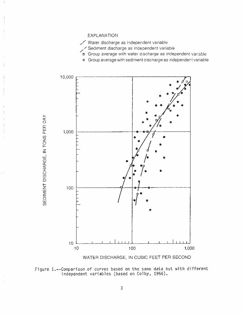
Sediment-transport curves should be constructed with sediment discharge as the dependent variable, Convention requi res the dependent variable be plotted as the ordinate. Figure 1, based on Colby (1956) , shows two curves derived with the same data b u t with different independent variables, The curve represented by the solid l ine assumes that water discharge i s the independent variable and thus should be used t o compute average sediment discharge for a given water discharge, The dashed curve of figure 1 assumes that water discharge i s the dependent variable and i s based on the average water discharge values for a small range in sediment discharge. I f there i s a wide sca t te r of points about th i s curve, i t s use may produce incorrect resul ts throughout the upper and/or the lower end of the curve. Upward or downward extension of the dashed curve will also give inaccurate sediment discharges.

The independent variables should not only be chosen correctly, b u t the variables should be expressed in meaningful terms. Water discharge should n o t be used direct ly as an independent variable for a relation t o be applied t o drainage basins of different s izes , b u t should be expressed as flow per unit area or as a ra t io t o average flow. The need for meaningful terms for the independent variables generally i s greater i f the defined relations are t o be applied a t more than one s i t e . Meaningful terms also are desirable for relations a t one s i t e .

Sediment-transport curves may be constructed with ei ther sediment concentration or sediment discharge as the dependent variable, In graphical analyses, the plot of sediment discharge against water discharge has less

EXPLANATION

F i g u r e 1.-

/ Water discharge as independent variable

/ Sediment discharge as independent variable

a Group average with water discharge as independent variable o Group average with sediment discharge as independent variable

10,000

1,000

100

10 10 100 1,000

WATER DISCHARGE, IN CUBIC FEET PER SECOND

-Comparison o f cu rves based on t h e same d a t a b u t w i t h d i f f e independent v a r i a b l es (based on Col by, 1956).

r e n t

s c a t t e r t h a n does t h e p l o t o f sediment c o n c e n t r a t i o n and can be b e t t e r f i t t e d b y eye. M a t h e m a t i c a l l y , however, t h e two re1 a t i o n s w i 11 produce i d e n t i c a l r e s u l t s (Rantz, %968), It i s a common p r a c t i c e t o c o n s t r u c t t h e t r a n s p o r t c u r v e i n t h e v a r i a b l e t h a t i s t o be es t ima ted ; t h a t i s , i f c o n c e n t r a t i o n s a r e t o be es t ima ted , t h e n t h e c u r v e i s c o n s t r u c t e d as c o n c e n t r a t i o n vs. w a t e r d i s c h a r g e and l i k e w i s e i f sediment d i s c h a r g e i s t o be es t ima ted , t h e n t h e sed iment d i s c h a r g e vs, w a t e r d i s c h a r g e f o r m i s used,

TYPES OF TRANSPORT CURVES

A s e d i m e n t - t r a n s p o r t c u r v e i s t h e c u r v e t h a t d e f i n e s t h e average r e l a - t i o n between sediment d i s c h a r g e and w a t e r d i scha rge . Acco rd ing t o Co lby (1956), s e d i m e n t - t r a n s p o r t c u r v e s may be c l a s s i f i e d a c c o r d i n g t o e i t h e r t h e p e r i o d o f t h e b a s i c d a t a t h a t d e f i n e s a c u r v e o r t h e k i n d o f sediment d i s - cha rge t h a t a c u r v e r e p r e s e n t s , S e d i m e n t - t r a n s p o r t cu rves based on t h e p e r i o d o f t h e b a s i c d a t a may be c l a s s i f i e d as i ns tan taneous , d a i l y , month ly , seasona l , annual , o r f l o o d - o r s t o r m - p e r i o d curves. The i n s t a n t a n e o u s s e d i m e n t - t r a n s p o r t cu rves a r e d e f i n e d by c o n c u r r e n t measurements o f sed iment d i s c h a r g e and w a t e r d i s c h a r g e f o r p e r i o d s t o o s h o r t t o be s u b s t a n t i a l l y a f f e c t e d by changes i n f l o w o r c o n c e n t r a t i o n d u r i n g t h e measurements. D a i l y , mon th l y , seasonal , annual , and f l o o d - p e r i o d s e d i m e n t - t r a n s p o r t cu rves u s u a l l y a r e d e f i n e d by and expressed as average sediment ( t o n s p e r day) and w a t e r d i s c h a r g e s ( c u b i c f e e t p e r second) f o r p e r i o d s o f days, months, y e a r s , o r s t o r m pe r iods , They can be d e f i n e d by and expressed as t o t a l q u a n t i t i e s o f sed iment ( t o n s ) and wa te r d i s c h a r g e s ( a c r e - f e e t ) d u r i n g t h e r e s p e c t i v e l e n g t h s o f t ime.

On t h e b a s i s o f t h e k i n d o f sediment t h a t t h e d a t a r e p r e s e n t , sed iment - t r a n s p o r t cu rves may be used t o d e f i n e t h e suspended-sediment l oad , unsampled- o r unmeasured-sediment l oad, bed1 oad, bed-mater i a1 1 oad, and t o t a l -sediment l oad . These t r a n s p o r t cu rves may be f u r t h e r s u b d i v i d e d a c c o r d i n g t o s i z e of p a r t i c l e s f o r wh ich t h e d e f i n i n g sediment d i s c h a r g e s were computed.

DEVELOPING A SEDIMENT-TRANSPORT CURVE

It s h o u l d be p o i n t e d o u t t h a t j u s t because a s t r a i g h t l i n e may be f i t t e d t h r o u g h a s e t o f p o i n t s , t h i s does n o t mean t h a t i t w i l l a c c u r a t e l y d e f i n e t h e r e l a t i o n between t h e v a r i a b l e s , Cons ider , f o r example, t h e c u r v e s shown i n f i g u r e 2, F i g u r e 2a shows an example o f how a s t r a i g h t l i n e was i n c o r r e c t l y f i t t o a much more complex r e l a t i o n , F i g u r e 2b i s an example o f where t h r e e s t r a i g h t l i n e c u r v e s wou ld much more a c c u r a t e l y d e f i n e t h e r e l a t i o n between x and y t h a n would a s i n g l e s t r a i g h t 1 i n e curve.

The sed imen t - t r a n s p o r t c u r v e i s normal l y p l o t t e d on 1 og paper. Commonly 5 by 3 l o g c y c l e paper i s used, w i t h t h e sediment d i s c h a r g e b e i n g p l o t t e d on t h e 5 - c y c l e s ide . I f a d d i t i o n a l c y c l e s a r e needed, t h e y may be c u t and s p l i c e d on. Use o f a s t a n d a r d l o g paper f a c i l i t a t e s compar ison o f p l o t s f rom d i f f e r e n t y e a r s a t t h e same s i t e and between d i f f e r e n t s i t e s .

Methods commonly used t o c o n s t r u c t t h e l i n e t h a t r e p r e s e n t s t h e r e l a t i o n between s t r e a m f l o w and sediment d i s c h a r g e i n c l u d e v i s u a l f i t 3 group average, and l i n e a r r e g r e s s i o n o f l o g - t r a n s f o r m e d data ,

INDEPENDENT VARIABLE x

INDEPENDENT VARIABLE x

F i g u r e 2.--Examples o f s i n g l e s t r a i g h t l i n e s n o t adequate ly d e f i n i n g t h e r e l a t i o n between dependent and i ndependent v a r i a b l e s .

To avo id m i s i n t e r p r e t a t i o n , a p r e l i m i n a r y g raph i ca l a n a l y s i s shou ld always be t h e f i r s t s t ep i n deve lop ing a sed iment - t ranspor t curve. Th i s g raph i ca l a n a l y s i s may revea l s i g n i f i c a n t re1 a t i o n s t h a t m igh t never be noted o r understood i f mathematical a n a l y s i s were a p p l i e d w i t h o u t a p r e l i m i n a r y ana l ys i s . A s imp le p l o t o f sediment d ischarge o r concen t ra t i on versus water d ischarge o f t e n w i l l i n d i c a t e whether t h e r e l a t i o n i s s imp le o r complex. I f t h e r e l a t i o n i s complex, examinat ion o f a p l o t o f t h e da ta may i n d i c a t e a r a t i o n a l method f o r a p p l y i n g a c o r r e c t mathematical s o l u t i o n . Some o f t h e ques t ions t h a t should be cons idered d u r i n g t h e p r e l i m i n a r y a n a l y s i s i nc l ude :

1. Should t h e r e l a t i o n be one o r more s t r a i g h t l i n e s o r a cu rve?

2. Are t h e da ta adequate t o e s t a b l i s h a r e l a t i o n ove r t h e e n t i r e range o f water d ischarge expected a t t h e s i t e be ing ra ted?

3. Do t h e da ta cover bo th d r y and wet per iods , w i n t e r and summer seasons, and a l l phases o f t h e hydrograph?

4. Are t h e r e a t y p i c a l yea rs o r events con ta ined i n t h e da ta which cou ld i n c o r r e c t l y b i a s t h e re1 a t i on?

5. E s p e c i a l l y a t t h e upper end o f t h e curve, a re t h e da ta r e p r e s e n t a t i v e o f a number o f events o r a re t hey p redominan t l y f rom a s i n g l e even t?

There a re severa l f a c t o r s t h a t can have an e f f e c t on t h e shape, s lope, and i n t e r c e p t of t h e sed iment - t ranspor t curve. Some o f t h e more major ones a re : ( 1 ) seasons, ( 2 ) t i m i n g between sediment concen t ra t i on peak and water d ischarge peak, and ( 3 ) extreme h igh-water events.

Seasons can have a s i g n i f i c a n t e f f e c t on sediment y i e l d , e s p e c i a l l y i n t h e more humid areas. Dur ing w i n t e r t h e ground may be f r o z e n and p r e c i p i t a - t i o n may be i n t h e form o f snow. As t h e snow mel ts , i t runs o f f t h e f r o z e n ground, The f a c t o r s o f (1) t h e absence o f r a i nd rop impact t o loosen t h e s o i l and ( 2 ) t h e f r ozen ground h o l d i n g t o g e t h e r b e t t e r , combine t o produce l owe r y i e l d s . Dur ing t h e summer when h i g h i n t e n s i t y storms a r e p reva len t , r a i n d r o p impact i s h i gh and t hus sediment concen t ra t i ons a re h igher . An a d d i t i o n a l comp l i ca t i on may a l s o occur where a l a r g e area o f t h e d ra inage b a s i n i s used f o r a g r i c u l t u r a l purposes, such as t h e Midwest. T y p i c a l l y t h e f i e l d s a re bare d u r i n g t h e w i n t e r and spr ing, b u t as t h e crops, such as corn, soybeans, and wheat, grow, t h e s o i l becomes p r o t e c t e d f rom e r o s i o n by t h e p l an t s . I n these cases, sediment y i e l d s f o r a g iven d ischarge may be low i n t h e w i n t e r ( f r o z e n ground) and summer ( h i g h c rops ) and h i g h e r i n t h e s p r i n g ( b e f o r e p l a n t i n g and growth o f t h e c rops) and f a l l ( a f t e r ha r ves t ) .

F i g u r e 3 i s an example o f d i f f e r e n c e s i n sediment y i e l d s between w i n t e r t y p e storms and summer t y p e storms (based on C u r t i s and o thers , 1978, p. 51). The two l i n e s f i t t e d t o t h e p o i n t s are- obv ious l y n o t we71 def ined. There i s a cons ide rab le amount o f s c a t t e r and even some ove r l ap between w i n t e r and summer t y p e storms, However, i t should be noted t h a t i t i s no t uncommon i n cases l i k e t h i s t o have a cons tan t s l ope t o t h e sed iment - t ranspor t curve, w i t h t h e seasonal e f f e c t o n l y be ing shown i n t h e y i n t e r c e p t . F i gu re 3 shows

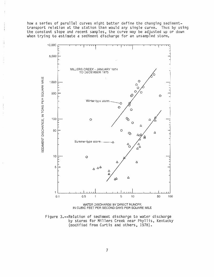
how a s e r i e s o f p a r a l l e l cu rves m i g h t b e t t e r d e f i n e t h e changing sediment- t r a n s p o r t r e l a t i o n a t t h e s t a t i o n t h a n would any s i n g l e curve. Thus by u s i n g t h e c o n s t a n t s l o p e and r e c e n t samples, t h e c u r v e may be a d j u s t e d up o r down when t r y i n g t o e s t i m a t e a sediment d i s c h a r g e f o r an unsampled storm.

WATER DISCHARGE BY DIRECT RUNOFF, IN CUBIC FEET PER SECOND-DAYS PER SQUARE MILE

F i g u r e 3 . - -Re la t ion o f sediment d i s c h a r g e t o w a t e r d i s c h a r g e by storms f o r M i l l e r s Creek near P h y l l i s , Kentucky ( m o d i f i e d f r o m C u r t i s and o t h e r s , 1978).

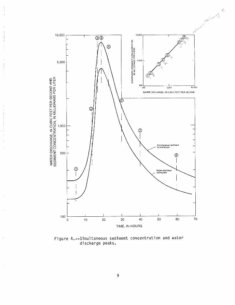
The t i m i n g between t h e sediment concen t ra t i on peak and t h e wate r d i s - charge peak can a l s o d r a s t i c a l l y a f f e c t t h e shape o f t h e sed iment - t ranspor t curve. F igures 4, 5, and 6 i l l u s t r a t e d t h i s e f f e c t . A l l t h r e e f i g u r e s have t h e same sur face-water hydrograph and sediment hydrograph. The o n l y change i s t h e t i m i n g o f t h e peak, I n f i g u r e 4 t h e sediment and water peaks co inc ide , i n f i g u r e 5 t h e sediment peak i s approx imate ly 5 hours ahead o f t h e water peak, and i n f i g u r e 6 t h e sediment peak l a g s t h e water peak by 5 hours. These f i g u r e s no t o n l y show how t h e t i m i n g o f t h e peaks can a f f e c t t h e shape o f t h e sed iment - t ranspor t cu rve b u t i t a l s o shows how t h e t i m i n g o f t h e samples can a f f e c t t h e r e s u l t s . I f samples were o n l y c o l l e c t e d on t h e peak and d u r i n g recess iona l pe r iods , no problem would be encountered i n f i g u r e 4; however, a t a s t a t i o n where c o n c e n t r a t i o n and water d ischarge peaks a re n o t c o i n c i d e n t , such as f i g u r e 5, a compl e t e l y erroneous curve m igh t be developed. I f no samples were c o l l e c t e d on t h e r i s e a t t h i s t y p e s t a t i o n , t hen o n l y samples such as 5-8 would be p l o t t e d . A t r a n s p o r t cu rve such as f i g u r e 7 would be drawn, and have ve ry l i t t l e s c a t t e r t o it. By n o t knowing what t h e r i s i n g hydrograph l ooks l i k e , a peak concen t ra t i on o f about 5,500 m i l l i g r a m s p e r l i t e r (mg/L) would be es t imated f o r t h i s s torm when t h e t r u e peak concen- t r a t i o n was 8,300 mg/b. The same t y p e o f problem can a r i s e when t h e sediment c o n c e n t r a t i o n peak l a g s t h e water d ischarge peak.

Q u i t e o f t e n a c a t a s t r o p h i c event w i l l s i g n i f i c a n t l y change t h e s l ope and/or shape o f t h e sed iment - t ranspor t curve. Kno t t (1971) presented f i g u r e 8 which shows sed iment - t ranspor t curves f o r t h e M idd le Fork Eel R i v e r below B lack B u t t e R i v e r near Covelo, Cal i f o r n i a , f o r t h e wa te r yea rs 1963-68. On December 22, 1964, a f l o o d hav ing an approximate reoccurrence i n t e r v a l o f 75 yea rs (Young and C r u f f , 1967) occur red a t t h i s s i t e . It i s apparent f rom f i g u r e 8 t h a t t h e 1964 f l o o d caused cons ide rab le change t o t h e sediment t r anspo r t -wa te r d ischarge r e l a t i o n . Even by 1968, t h e upper end o f t h e t r a n s p o r t cu rve had no t r e t u r n e d t o i t s p r e - f l o o d p o s i t i o n .

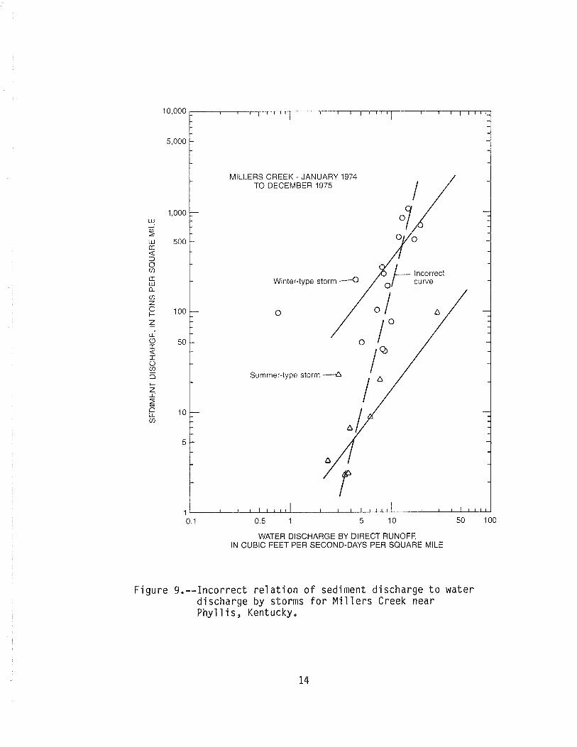
Another ma jo r problem one can encounter i n c o n s t r u c t i n g sediment- t r a n s p o r t curves i s when i n s u f f i c i e n t samples have been c o l l e c t e d t o d e f i n e t h e curve. Consider t h e example shown i n f i g u r e 9. These a re t h e same da ta as p resen ted i n f i g u r e 6 e a r l i e r b u t w i t h fewer samples shown, A casual l o o k a t t h e p l o t t e d da ta would suggest t h a t t h e dashed l i n e would n o t be a bad f i t o f t h e data. However, as shown i n f i g u r e 3, t h e dashed l i n e would be i n c o r - r ec t . One way t o h e l p avo id t h i s k i n d o f e r r o r i s t o p l o t a l l t h e da ta f o r a s t a t i o n f o r t h e p e r i o d o f record. Subsequent s u b d i v i s i o n s by season o r r i s i n g o r f a l l i n g t r e n d s can t hen be analyzed. A t p e r i o d i c a l l y sampled s t a t i o n s , i t may t a k e severa l yea rs o f da ta c o l l e c t i o n t o o b t a i n s u f f i c i e n t samples t o adequate ly d e f i n e a sed iment - t ranspor t curve.

SU

SP

EN

DE

D-S

ED

IME

NT

CO

NC

EN

TR

AT

ION

, IN

MIL

LIG

RA

MS

PE

R L

ITE

R

1

-I

0

DAILY MEAN WATER DISCHARGE, IN CUBIC FEET PER SECOND

F i g u r e 8,--Relat ion o f suspended-sediment d ischarge t o wa te r d ischarge a t M idd le Fork Eel R i v e r be1 ow B lack B u t t e R i v e r near Covelo, C a l i f o r n i a , 1963-68 water yea rs (Kno t t , 1971).

MILLERS CREEK - JANUARY 1974 TO DECEMBER 1975

winter-type storm -4 ,?.E % orrect v e

WATER DISCHARGE BY DIRECT RUNOFF, IN CUBIC FEET PER SECOND-DAYS PER SQUARE MILE

F i g u r e 9 . - - Incor rec t r e l a t i o n o f sediment d ischarge t o wa te r d ischarge by storms f o r M i l l e r s Creek near P h y l l i s , Kentucky.

VISUAL F IT

A l i n e drawn th rough t h e da ta p o i n t s , v i s u a l l y , t h a t appears t o represen t t h e b e s t average o r " f i t " i s r e f e r r e d t o as a v i s u a l f i t . It i s p robab ly t h e s i m p l e s t method o f c o n s t r u c t i n g a sed iment - t ranspor t cu r ve and f o r m e r l y was, and perhaps s t i l l i s , t h e most common procedure, F i gu re 10 i s an example o f a sed iment - t ranspor t cu rve drawn by eye. When t h e da ta a r e t i g h t l y grouped as i n f i g u r e 10, f i t t i n g t h e cu rve i s no t much o f a problem. However, even i f t h e da ta do n o t s c a t t e r much, t h e a n a l y s t should be aware o f t h e problems d iscussed i n t h e p rev i ous sec t ions . The da ta p o i n t s shou ld be l a b e l e d as t o da te o f c o l l e c t i o n and t i m i n g r e l a t i v e t o t h e water peak ( t h a t i s , r i s e , peak, o r f a l l i n g ) so t h a t a b e t t e r a n a l y s i s o f t h e da ta s e t can be made,

LINEAR REGRESSION

A l i n e a r r eg ress i on equa t ion ( l e a s t square) p rov ides a l i n e about which t h e sum o f t h e squares o f t h e dev ia t i ons , t h a t i s , t h e d i f f e r e n c e between t h e l i n e va l ue and t h e observed va lue i s a minimum,

I f t h e r e l a t i o n between sediment d ischarge and water d i scha rge da ta on l o g a r i t h m i c paper i s l i n e a r , t h i s r e l a t i o n may be expressed i n t h e fo rm o f

b Qs = aQ o r Log Qs = Log a + b Log Q ( 1 )

where Qs i s sediment d ischarge, i n tons pe r day; Q i s water d ischarge i n c u b i c f e e t pe r second; and a and b a re constants . The cons tan ts a and b a re so l ved by a p p l y i n g t h e equat ions f o r a s imp le l i n e a r r eg ress i on (Riggs, 1968, p. 11) t o l o g a r i t h m i c t rans fo rmed va lues o f water d ischarge and sediment d ischarge. The equa t ions a re

b =

c ( l o g Q ) Z - N ( r n ) 2

l o g a = l o g Qs - b l o g Q

.- -- and a = 10(10!3 Qs - b l o g Q)

where l o g Q = average o f water d ischarge va lues ( l o g a r i t h m s ) ,

l o g Qs = average o f sediment d ischarge va lues ( l o g a r i t h m s ) , and

N = number o f p a i r e d observat ions.

Standard s t a t i s t i c a l computat ions showing how w e l l t h e da ta f i t t h e equa t ion such as t h e square o f t h e c o r r e l a t i o n c o e f f i c i e n t ( r 2 ) , va r i ance o f X (s:), va r i ance o f y ( s 2 ) $ and s tandard e r r o r o f es t ima te (Sy,,) can be found i n Riggs (1968, p. 11) o r most o t h e r books on s t a t i s t i c s . (Note: The s t a t i s - t i c a l va lues computed d u r i n g t h e reg ress i on a n a l y s i s a r e based on t h e l o g a r i t h m i c va lues and t h e r e f o r e do n o t min imize t h e sum o f t h e squared d e v i a t i o n s o f t h e a c t u a l da ta f rom t h e reg ress i on l i n e . )

F i g u r e


10,--Instantaneous sediment- t ranspor t cu rve f i t t e d by eye (mod i f i ed from Jones and Ewart, 1973).

Regression equa t ions f o r sediment c o n c e n t r a t i o n versus water d ischarge can be p u t i n t o a s i m i l a r form as those f o r sediment d ischarge.

I f t h e equa t ion

which i s used t o compute sediment d ischarge f rom sediment concen t ra t i on i s s u b s t i t u t e d i n t o equa t ion 1, t h e r e l a t i o n between sediment concen t ra t i on and water d i scha rge becomes

where C = sediment concen t ra t ion , i n m i l l i g r a m s per l i t e r , a ' = a/.0027, and b ' = b - 1.

The use o f t h e l i n e a r r eg ress i on method g e n e r a l l y i s p r e f e r r e d over t h a t o f t h e v i s u a l method i f t h e p r e l i m i n a r y a n a l y s i s i n d i c a t e s t h a t t h e t r a n s p o r t cu rve can be represen ted by f o u r o r l e s s s t r a i g h t l i n e s .

Several au thors have r e c e n t l y expressed concern about fundamental s t a t i s - t i c a l b i a s i n l o a d es t imates f rom r a t i n g curves, p a r t i c u l a r l y when t h e curves a re e s t a b l i shed by 1 i n e a r r eg ress i on on 1 og-transformed da ta (Ferguson, 1986; Koch and S m i l l i e , 1986). The b i a s can be s u b s t a n t i a l i f t h e s tandard e r r o r o f t h e l o g - r e s i d u a l s i s l a rge ; Ferguson r e p o r t s sys temat i c underes t imat ion by as much as 50 percent . It i s o f t e n d e s i r a b l e t o e l i m i n a t e such b i as , and t h e papers ( i ndependen t l y ) suggest a method f o r o b t a i n i n g unbiased est imates, However, t h e c o r r e c t i o n t h e y recommend i s s e r i o u s l y f lawed, and may exacerbate t h e problem o f b i a s r a t h e r than so l ve it (T. A. Cohn, w r i t t e n commun., 1987). The exac t s o l u t i o n t o t h e s t a t i s t i c a l problem when e r r o r s a re norma l l y d i s t r i - buted i n l o g space i s p rov i ded by Bradu and Mundlak (1970). Another p o s s i b l e s o l u t i o n i s proposed by Duan (1983), which does no t depend on any d i s t r i b u - t i o n a l assumption. However, no c a r e f u l e m p i r i c a l a n a l y s i s has been made t o da te on t h e performance o f any o f these s o l u t i o n s t o t h e problem. I f care i s taken t o ensure t h e t r a n s p o r t curves a r e f i t t e d th rough t h e p o i n t s a t t h e h i g h end o f t h e cu r ve and t h e var iance o f t h e r e s i d u a l s i s smal l , e r r o r s i n e s t i m a t i n g sediment d ischarges caused by t h i s b i a s shou ld be smal l ,

Examples o f L i nea r Regression Method

The f o l l o w i n g a re examples o f how t o compute sed iment - t ranspor t curves us i ng t h e l i n e a r r eg ress i on technique. The examples used a re f o r streams t y p i c a l o f t h e P a c i f i c Slope Region o f t h e western U n i t e d S ta tes (Eel R i v e r a t Sco t ia , C a l i f o r n i a ) and t h e Piedmont Region o f t h e eas te rn Un i t ed S ta tes (Yadk in R i v e r near Yadkin Co1 lege, Nor th Ca ro l i na ) . Sediment d ischarges es t imated by u s i n g t h e reg ress i on equa t ion a re compared w i t h h i s t o r i c a l records t o i l l u s t r a t e t h e accuracy o f t h e method.

Eel R i v e r a t Sco t ia , Ca1 i f o r n i a

I n t h i s example, 29 samples o f suspended-sediment concen t ra t i on and wate r d ischarge ob ta i ned a t Eel R i v e r a t Sco t ia , C a l i f o r n i a , d u r i n g t h e 1958-60 water years a re used. The procedure f o r d e f i n i n g t h e t r a n s p o r t cu r ve us i ng t h e l i n e a r r eg ress i on method i s as f o l l o w s :

Step 1. L i s t ins tantaneous wate r d ischarge and concen t ra t i on da ta i n c h r o n o l o g i c a l o rder ( t ab1 e 1).

Step 2. Compute sediment d ischarge u s i n g equa t ion 5, C o l e 5 = 0,0027 x co l , 3 x c o l . 4.

Step 3, P l o t water d ischarge (absc issa) and sediment d ischarge ( o r d i n a t e ) on l o g a r i t h m i c paper ( f i g . k l ) ,

Step 4. Analyze t h e p l o t t e d da ta t o determine i f a s t r a i g h t l i n e c o u l d reasonably be f i t t e d t o p a r t o r t h e e n t i r e range o f p l o t t e d values, The a n a l y s i s should beg in w i t h t h e upper p a r t o f t h e graph. These d a t a a re most impo r tan t because t hey o f t e n represen t t h e ma jo r f r a c t i o n o f sediment t r a n s - p o r t e d i n a g iven y e a r and because t hey represen t t h e maximum va lues o f measured sediment discharge, Also, o f t e n t h e t r a n s p o r t cu rve must be e x t r a p o l a t e d beyond t h e sampled da ta t o es t ima te sediment d ischarge d u r i n g yea rs o f ex t reme ly h i g h d ischarge. I n t h i s example, i t appears t h a t a s t r a i g h t l i n e cou ld be f i t t e d f o r f l o w s rang ing f rom about 20,000 t o 150,000 c u b i c f o o t pe r second ( f t 3 / s ) . Examinat ion o f t h e da ta f o r f l ows l e s s t han 20,000 f t 3 / s i n d i c a t e s t h a t s t r a i g h t l i n e s cou ld be f i t t e d f o r t h e range 2,000 t o 20,000 f t 3 / s and p o s s i b l y another s t r a i g h t l i n e f o r d i scharges l e s s t han 2,000 f t3 /s . I n genera l , 10 o r more da ta p o i n t s per l o g c y c l e o f wa te r d ischarge a r e needed t o d e f i n e adequate ly a sed iment - t ranspor t curve.

A f t e r making a pre1imina:ry a n a l y s i s o f t h e a v a i l a b l e data, i t was dec ided t o compute r eg ress i on equa t ions f o r t h r e e ranges o f f l ow- -h igh f l o w (20,000 t o 1,51,0000 f t 3 / s ) , medium f l o w (2,000 t o 20,000 f t 3 / s ) , and Sow f l o w (98 t o 2,000 f t 3 / s ) . It may be d e s i r a b l e t o ove r l ap t h e end p o i n t s and t o use some o f t h e same da ta p o i n t s t o d e f i n e two ad jacen t s e c t i o n s o f t h e separate r eg ress i on 1 i nes.

Step 5, L i s t t h e da ta i n groupings f o r t h e computat ion o f each reg res - s i o n equa t ion ( t a b l e 2).

Step 6. Transform water d ischarge and sediment d ischarge t o l o g a v i t h m i c e q u i v a l e n t s (columns 4 and 6, t a b l e 2) .

Step 7. Compute averages, sums, and p roduc ts o f l o g a r i t h m i c equ i va l en t s .

Step 8. Compute t h e exponent b ( s l o p e o f l i n e ) us i ng equa t ion 2 and t h e i n t e r c e p t by u s i n g equa t ion 4; a and b a r e u s u a l l y computed t o t h r e e s i g n i f i - can t f i g u r e s , The cons tan ts f o r t h e t h r e e f l o w ranges are:

cn

WW

P

-4 w -03

r w

c

nO

PW

03

O

OO

NO

N orr

Ln

r

WW

03

r

-o

mo

m~

~~

U

U

mo

o

No

r

mo

o

e

0

V P

r ct)


F igu re 11.--Sediment-transport cu rve f o r Eel R i v e r a t Sco t ia , Cal i f o r n i a, 1958-60 water years.

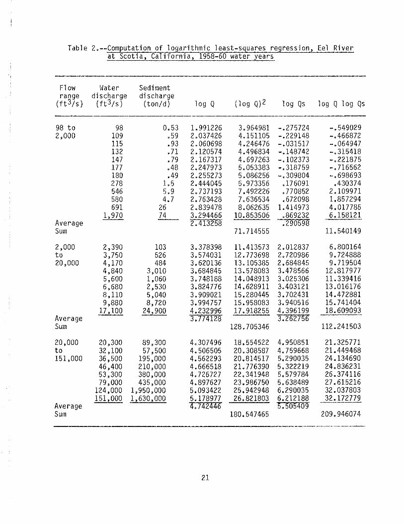
Table 2.--Computation o f a t Sco t ia , C a l i f o r n i a , 1958-60 wate r years

Flow Water Sediment range d ischarge d ischarge

( f t 3 / s ) ( f t 3 / s ) ( t on /d ) l o g Q ( I Q ~ Q ) ~ l o g Q s l o g Q l o g Q s

98 t o 2,000

Average Sum

2,000 t 0 20,000

Average Sum

20,000 t 0 151,000

Average Sum

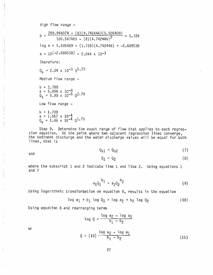
High f low range -

l o g a = 5.505409 - (1.728)(4.742446) = -2.689538

Therefore:

Medium f l o w range -

Low f l o w range -

Step 9. Determine t h e exac t range o f f l o w t h a t a p p l i e s t o each regres - s i o n equat ion. A t t h e p o i n t where two ad jacen t r eg ress i on l i n e s converge, t h e sediment d ischarge and t h e water d ischarge va lues w i l l be equal f o r bo th l i n e s , t h a t i s

and

where t h e s u b s c r i p t 1 and 2 i n d i c a t e l i n e 1 and l i n e 2. Using equat ions 1 and 7

Us ing l o g a r i t h m i c t r a n s f o r m a t i o n on equa t ion 9, r e s u l t s i n t h e equa t ion

Us ing equa t ion 8 and rea r rang ing terms

l o g a2 - l o g a 1 l o g Q =

"1 - "2

l o g a2 - l o g a1 Q = (10)

The p o i n t of convergence between t h e h i g h and medium f l o w regress ion l i n e s occurs a t

l o g Q = = 4.315382

and t h e p o i n t o f convergence between medium and low f l o w occurs a t

l o g Q = = 3.70551

Thus, t h e range o f f l o w f o r each regress ion equat ion i s

Three regress ion equat ions gene ra l l y a re needed t o comple te ly d e f i n e a sediment -t ranspor t re1 a t i on a t a g i ven s i t e . The re1 a t i on i n d i cated i n f i g u r e 11 i s t y p i c a l o f many s i t e s , i n t h a t t h e s lopes f o r h i g h and low f l o w a r e g e n e r a l l y l e s s than t h a t f o r medium f low.

Yadkin R i v e r a t Yadkin Col lege, Nor th Ca ro l i na

Data used i n t h i s example a re 39 p e r i o d i c samples o f suspended-sediment concen t ra t i on and water d ischarge f o r Yadkin R i ve r a t Yadkin Col lege, Nor th Caro l i n a ( t a b l e 3). Exp lana to ry and computat ion s teps have been om i t t ed because they have been descr ibed i n t h e p rev ious example.

An a n a l y s i s o f t h e da ta p l o t t e d i n f i g u r e 12 i n d i c a t e s t h a t a r e r e s s i o n 4 l i n e cou ld be f i t t e d t o t h e values f o r d ischarges l e s s than 15,000 ft /s. A t h i g h e r discharges, however, t h e p o i n t s a re w ide l y s c a t t e r e d and no c l e a r r e l a t i o n i s apparent.

Several approaches can be used t o d e f i n e a r e l a t i o n f o r t h e upper p a r t o f t h e graph. One would be t o extend t h e regress ion l i n e developed f o r d i s - charges l e s s than 15,000 f t 3 / s t o i n c l u d e t h e h i g h f l o w range. Th is exten- s i o n i s shown as t h e dashed l i n e i n f i g u r e 12, This may o r may n o t be an accura te rep resen ta t i on o f t h e sediment t r a n s p o r t r e l a t i o n a t h i g h f l o w s f o r t h i s s t a t i o n . Another approach t o develop ing t h e sediment- t ranspor t curve f o r d ischarges above 15,000 f t 3 / s would be t o t a k e a l o g i c a l look a t t h e data po in t s , keeping i n mind some o f t h e t h i n g s discussed e a r l i e r t h a t cou ld a f f e c t t h e shape o f t h e t r a n s p o r t curve. To t h e l e f t o f t h e dashed l i n e l i e s a group o f p o i n t s between 16,000 and 22,000 f t 3 / s e Four o f these p o i n t s were c o l l e c t e d d u r i n g a s i n g l e s torm event. A p l o t o f these p o i n t s ( f i g . 13) shows t h a t t h e sediment concen t ra t i on peaked about 13 hours p r i o r t o t h e water d ischarge peak o f 22,100 f t 3 / s a t 2,230. We saw e a r l i e r t h a t a stream

Table 3,--Instantaneous suspended-sediment and water discharge, Yadkin R i v e r a t Yadkin Col lege, Nor th Caro l ina, 1969-73 water years

Water Sediment Sediment d ischarge concent r a t i on d ischarge

Date T i me ( f t 3 / s ) (mg/L) ( t on /d ) ( 1 ) ( 2 ) ( 3 ( 4 ) ( 5 )


F igu re 12.--Relat ion between sediment d ischarge and wate r d ischarge u s i n g l i n e a r r eg ress i on method, Yadkin R i v e r a t Yadkin Col lege, Nor th Caro l ina , 1969-73 wate r years.

23,000

YADKIN RIVER Cr YADKIN COLLEGE, N.C. FEBRUARY 23, 1971

22,000

21,000

20,000

19,000 3000

18,000 2500

17,000 2000

16,000 1500

TIME, IN HOURS

F igu re 13.--Water d ischarge and sediment concen t ra t i on hydrographs f o r Yadkin R i v e r a t Yadkin Col lege, Nor th Caro l ina, f o r February 23, 1971,

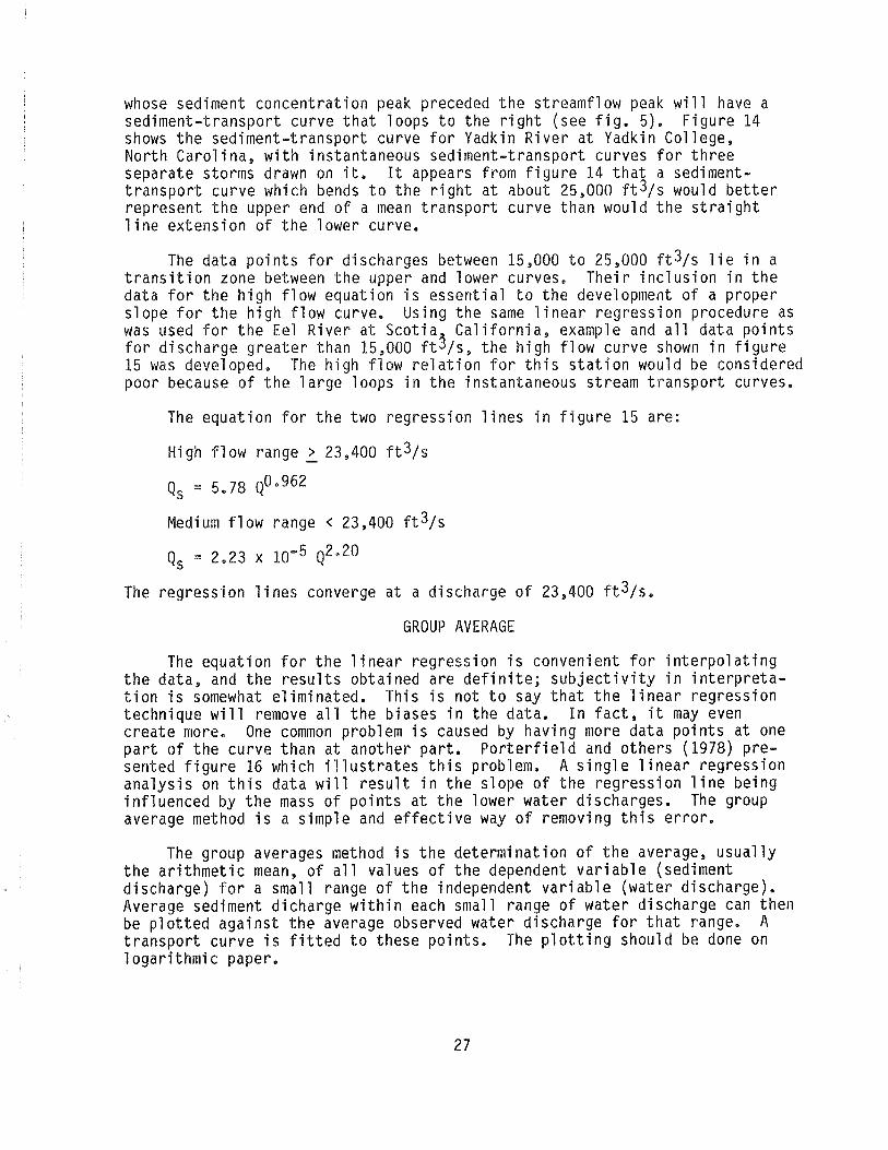
whose sediment concen t ra t i on peak preceded t h e s t reamf low peak w i l l have a sed iment - t ranspor t cu rve t h a t loops t o t h e r i g h t (see f i g . 5). F i g u r e 14 shows t h e sed iment - t ranspor t cu rve f o r Yadkin R i v e r a t Yadkin Col lege, Nor th Ca ro l i na , w i t h ins tantaneous sed iment - t ranspor t curves f o r t h r e e separate storms drawn on it. It appears f rom f i g u r e 14 t h a t a sediment- t r a n s p o r t cu r ve which bends t o t h e r i g h t a t about 25,000 f t 3 / s would b e t t e r represen t t h e upper end o f a mean t r a n s p o r t cu r ve t han would t h e s t r a i g h t 1 i n e ex tens ion o f t h e 1 ower curve.

The da ta p o i n t s f o r d ischarges between 15,000 t o 25,000 f t 3 / s l i e i n a t r a n s i t i o n zone between t h e upper and lower curves. T h e i r i n c l u s i o n i n t h e da ta f o r t h e h i g h f l o w equa t ion i s e s s e n t i a l t o t h e development o f a p roper s l ope f o r t h e h i g h f l o w curve, Us ing t h e same l i n e a r r eg ress i on procedure as was used f o r t h e Eel R i v e r a t S c o t i a C a l i f o r n i a , example and a l l da ta p o i n t s

3 f o r d i scharge g r e a t e r than 15,000 ft I s , t h e h i g h f l o w cu rve shown i n f i g u r e 15 was developed. The h i g h f l o w r e l a t i o n f o r t h i s s t a t i o n would be cons idered poor because o f t h e l a r g e loops i n t h e ins tan taneous stream t r a n s p o r t curves.

The equa t i on f o r t h e two reg ress i on l i n e s i n f i g u r e 15 are:

High f l o w range - > 23,400 f t 3 / s

Qs = 5,78 Q 0,962

Medium f l o w range < 23,400 f t 3 / s

The reg ress i on 1 i nes converge a t a d ischarge o f 23,400 f t 3 / s .

GROUP AVERAGE

The equa t i on f o r t h e l i n e a r r eg ress i on i s conven ien t f o r i n t e r p o l a t i n g t h e data, and t h e r e s u l t s ob ta ined a re d e f i n i t e ; s u b j e c t i v i t y i n i n t e r p r e t a - t i o n i s somewhat e l im ina ted . Th is i s no t t o say t h a t t h e l i n e a r r eg ress i on techn ique w i l l remove a19 t h e b iases i n t h e data. I n f a c t , i t may even c r e a t e more. One common problem i s caused by hav ing more da ta p o i n t s a t one p a r t o f t h e cu r ve t han a t another pa r t . P o r t e r f i e l d and o t h e r s (1978) p re - sented f i g u r e 16 which i l l u s t r a t e s t h i s problem. A s i n g l e l i n e a r r eg ress i on a n a l y s i s on t h i s da ta w i l l r e s u l t i n t h e s lope o f t h e r eg ress i on l i n e be ing i n f l u e n c e d by t h e mass o f p o i n t s a t t h e lower wa te r d ischarges. The group average method i s a s imp le and e f f e c t i v e way o f removing t h i s e r r o r .

The group averages method i s t h e de te rm ina t i on o f t h e average, u s u a l l y t h e a r i t h m e t i c mean, o f a l l va lues o f t h e dependent v a r i a b l e (sediment d ischarge) f o r a smal l range o f t h e independent v a r i a b l e (wa te r d ischarge) . Average sediment d i cha rge w i t h i n each smal l range o f wa te r d ischarge can t hen be p l o t t e d a g a i n s t t h e average observed water d i scha rge f o r t h a t range. A t r a n s p o r t cu r ve i s f i t t e d t o these po in t s . The p l o t t i n g should be done on l oga r i t hm ic paper.

1,000,000

>- R = Rising Stage Q 0 F = Falling Stage 0 CT W 100,000 a V) z 0 t-

z w (3 a Q I 0 cn 10,000 Cl I- Z W

r n W V)

I n W Cl z 1,000 W a a 3 cn

100


F igu re 14.--Relation between sediment d ischarge and water d ischarge f o r t h r e e peaks on Yadkin R i v e r a t Yadkin Col lege, Nor th Caro l ina.


F i g u r e 15.--Best es t imate o f t h e r e l a t i o n between sediment d ischarge and water discharge, Yadkin. R i v e r near Yadkin Col lege, Nor th Carol i na, 1969-73 water years.

WATER DISCHARGE. IN CUBIC FEET PER SECOND

F i gure 16. --Re1 a t i on between s t reamf 1 ow and suspended- sediment discharge, Feather R i v e r a t Orov i l l e , C a l i f o r n i a , 1958 water yea r ( P o r t e r f i e l d and o thers , 1978).

Th i s example uses t h e Eel R i v e r a t S c o t i a da ta used f o r t h e l i n e a r r eg ress i on method. The procedure i s as f o l l o w s :

Step 1. L i s t water d ischarge and concen t ra t i on da ta i n ch rono log i ca l o r d e r ( t a b l e I),

Step 2. Compute sediment d ischarge u s i n g equa t ion 5. Col. 5 = 0,0027 x Col. 3 x Col. 4,

Step 3. P l o t water d ischarge (absc i ssa ) and sediment d ischarge ( o r d i n a t e ) on l o g a r i t h m i c paper ( f i g . 11).

Step 4. Analyze t h e p l o t t e d da ta f o r unusual o r anomalous c l u s t e r s o f d a t a p o i n t s and obv ious o u t l i e r s . I F unusual o r o u t l i e r da ta e x i s t , t h e y shou ld be rechecked f o r p o s s i b l e e r r o r s (sampl i ng, 1 abora to ry , o r computat ion) and f o r cause. A l a r g e number o f samples c o l l e c t e d d u r i n g a s h o r t p e r i o d may be r e p r e s e n t a t i v e o f c o n d i t i o n s ( c o n s t r u c t i o n , seasonal e f f e c t s , w i 1 d f i r e s ) t h a t would b i a s t h e use o f t h e t r a n s p o r t cu rve f o r e s t i m a t i n g long- te rm cond i - t i o n s . The p r e l i m i n a r y a n a l y s i s f o r t h e group averages method u s u a l l y i s m inor because t h e r e l a t i o n i s averaged f o r many smal l increments o f s t reamf low.

Step 5. Arrange water -d ischarge va lues i n t o un i f o rm groups' o r c l asses acco rd i ng t o magnitude ( t a b l e 4). Extremes f o r each group ( c l a s s l i m i t s ) can usual l y be ob ta ined f rom ava i 1 a b l e f l ow -du ra t i on t a b l es where d a i l y d i scha rge i s d i s t r i b u t e d i n t o about 30 groups. Fewer groups a r e j u s t i f i e d i f t h e da ta s e t i s smal l .

For example, t o o b t a i n 15 groups f o r t h e 1958-60 water years , t h e procedures woul d be:

1. Se lec t t h e upper and l owe r c l a s s l i m i t s . Se lec t t h e l owe r c l a s s l i m i t j u s t sma l l e r than t h e minimum f o r t h e p e r i o d and t h e maximum c l a s s 1 i x i mum observed d a i l y d ischarge f o r t h e Fo r t h i s example, use 70 and 170,000 f t 3 / s .

2. Determine t h e d i f f e r e n c e o f t h e l oga r i t hms o f t h e minimum and maximum c l a s s l i m i t s ,

Log 170,000 - l o g 70 = 5.230449 - 1.845098 = 3.385351

3, D i v i d e t h e d i f f e r e n c e by t h e number o f groups ( t h a t i s , 15) minus one.

4, Increment t h e l o g a r i t h m o f each success ive c l a s s l i m i t by 0.241811 and determine t h e a n t i l o g a r i t h m (minimum d ischarge o f t h e group).

Group Log A n t i 1 og (rounded)

Step 6. L i s t i n d i v i d u a l water d ischarges and assoc ia ted sediment d i s - charges i n groups ranked i n ascending o r descending o rde r o f water discharge. For streams where a s i g n i f i c a n t f r a c t i o n o f t h e annual sediment l oad i s t r a n s p o r t e d i n a few days, l i s t severa l o f t h e l a r g e s t d ischarge values i n d i v i d u a l l y t o more p r e c i s e l y d e f i n e t h e upper end o f t h e t r a n s p o r t curve.

Step 7. Compute t h e a r i t h m e t i c mean o f t h e wate r d ischarges and sed i - ment d ischarges f o r each group.

Step 8. P l o t t h e group averages' on l o g a r i t h m i c paper ( f i g . 17).

Step 9. The sediment- t ranspor t curve can be ob ta ined f rom t h e group average p o i n t s by two methods: (1) by j o i n i n g t h e p o i n t s w i t h a s t r a i g h t l i n e between p o i n t s o r ( 2 ) by develop ing a cu rve (s ) , u s i n g t h e p o i n t s as a guide.

The dashed l i n e i n f i g u r e 17 shows a sed iment - t ranspor t curve drawn u s i n g t h e f i r s t method. Several problems a r i s e f rom t h i s method. The sed i - ment d ischarge appa ren t l y decreases w i t h i n c r e a s i n g wate r d ischarge between p o i n t s 1 and 2 and t h e s i n g l e po in t s , such as 5 and 11, may cause d r a s t i c changes i n slope. For these reasons, i t i s g e n e r a l l y p e r f e r r e d t o use t h e second method t o d e f i n e t h e sediment- t ranspor t cu rve f rom t h e group average po in t s . The s o l i d l i n e i n f i g u r e 17 was developed u s i n g t h e group average p o i n t s and a l i n e a r regress ion ana lys is , and d i v i d i n g t h e curve i n t o t h r e e s t r a i g h t l i n e segments. The l i n e a r regress ion a n a l y s i s method used was t h e same as t h a t d iscussed i n t h e p rev ious sec t ion , w i t h t h e excep t ion t h a t t h e group average p o i n t s were used i n s t e a d o f t h e i n d i v i d u a l da ta po in t s .

Table 4.--Computation o f sediment- t ranspor t r e l a t i o n us ing group averages, Eel R i ve r a t Scot ia , C a l i f o r n i a , 1958-60 water years

Class l i m i t Water d ischarge Sediment d ischarge Group ( f t 3 / s ( f t 3 / s ) ( t on /d )

Data Mean Data Mean

The equat ion and range o f f l o w f o r t h e regress ion equat ions based on t h e group average da ta are:

Q < 1980 f t 3 / s , Q, = 1.02 x l oe4 Q


F i g u r e 17,--Sediment-transpQrt curves based on group averages method f o r Eel R i v e r a t Sco t i a , C a l i f o r n i a , 1958-60 water years,

Another major advantage o f u s i n g a l i n e a r r eg ress i on a n a l y s i s on t h e group average p o i n t s i s t h a t t h e s l ope o f t h e upper end o f t h e t r a n s p o r t cu rves i s d e f i n e d b e t t e r . A s l i g h t e r r o r i n t h e s l ope a t t h e upper end o f t h e cu rve can mean a s i g n i f i c a n t d i f f e r e n c e i n t h e es t imated sediment d i s - charge. For example, i f t h e sediment d ischarge f o r a water d ischarge o f 200,000 f t 3 / s was t o be es t imated f rom t h e curves i n f i g u r e 17, t h e f i r s t method (dashed l i n e ) would produce an es t imated sediment d ischarge o f 4.5 m i l l i o n t ons pe r day, Us ing t h e s o l i d l i n e , t h e es t imated sediment d ischarge would be 3.0 m i l l i o n t ons pe r day, Th is d i f f e r e n c e may be very s i g n i f i c a n t when we cons ider t h a t f o r most streams t h e m a j o r i t y o f t h e sediment i s t r a n s - p o r t e d i n a few days, The 1.5 m i l l i o n tons pe r day d i f f e r e n c e i n t h i s example may be e q u i v a l e n t t o 40 o r 50 percen t o f t h e t o t a l sediment d ischarge f o r t h e year .

OTHER PROBLEMS ASSOCIATED WITH COMPUTER-FITTED CURVES

Several o t h e r problems can a r i s e when computer programs a r e used t o compute sed iment - t ranspor t curves. Jus t because a cu rve " f i t s " t h e da ta p o i n t s , i t does n o t n e c e s s a r i l y make i t h y d r a u l i c l y c o r r e c t . The f o l l o w i n g i s a d i scuss ion o f severa l o f t h e more common types o f problems encountered when us i ng computers t o generate sed iment - t ranspor t curves.

Table 5 and f i g u r e 18 show d a i l y sediment d ischarges f o r a summer peak on a smal l stream i n Pennsylvania, arrows show t h e p rog ress i on o f t h e s to rm days, F igures 19 and 20 a r e p l o t s o f t h e same storm w i t h t h e s tandard l i n e a r r eg ress i on and l og -quad ra t i c equat ions f i t t o t h e p o i n t s r e s p e c t i v e l y , Both

Table 5,- f i a u r e s 18-21 and 24 a r e based on

Flow Load f t v s t o n

DISCHARGE. IN CUBIC FEET PER SECOND

Figure 18.--Daily sediment discharge for a summer peak on a small stream in Pennsylvania.

1 o1 1 02 1 o3

DISCHARGE, IN CUBIC FEET PER SECOND

F i g u r e 19.--Sediment-transport cu rve based on 1 og-1 i near r eg ress i on ana l ys i s ,


F i g u r e 20.--Sediment-transport cu rve based on l og -quad ra t i c r eg ress i on ana l ys i s .

show good c o r r e l a t i o n ( h i g h ~2 va lues) and low s tandard e r r o r s ( s ) . The 1 i nea r - r eg ress i on curve ( f i g . 19) underest imates t h e peak whereas t h e curve i n f i g u r e 20 comes very c l o s e t o c o r r e c t l y e s t i m a t i n g t h e peak sediment discharge. However, i f we examine t h e curve i n f i g u r e 20 more c l o s e l y , we see two ma jo r problems w i t h i t: ( 1 ) a t t h e lower end i t shows an i nc rease i n sediment d ischarge w i t h decreas ing water d ischarge; and ( 2 ) t h e upper end o f t h e cu rve i s c u r v i n g upward, thus showing eve r - i nc reas ing sediment d ischarge w i t h i n c r e a s i n g water discharge. The u l t i m a t e r e s u l t o f t h e second problem would be t h a t w i t h ve ry l i t t l e i nc rease i n water d ischarge, we would have a ve ry l a r g e i nc rease i n sediment d ischarge, The curve i n f i g u r e 20 does have l i m i t e d uses, however, and can be used i f t h e range o f d i scharge i s equiva- l e n t t o t h e range d e f i n e d by t h e da ta po in t s . Th is does n o t h e l p when t r y i n g t o es t ima te sediment d ischarges o u t s i d e t h i s range, e s p e c i a l l y a t t h e upper end. I n t h i s p a r t i c u l a r case, two curves migh t be b e t t e r than one f o r e s t i - mat ing sediment discharges. F i g u r e 21 shows two curves t h a t m igh t be used, t h e upper cu rve t o be used on r i s i n g and peak days, t h e l owe r one f o r reces- s i o n a l days. Table 6 g ives t h e peak sediment d ischarges es t imated us i ng t h e curves shown i n f i g u r e s 19, 20, and 21.

Table 6.- i n t ons pe r dav f o r i n d i c a t e d

Double s t r a i g h t 2,620 18,000 l i n e

*Actua l peak sediment d ischarge recorded.

F i gu re 20 a1 so i 11 u s t r a t e s t h e problem w i t h computer-generated sediment- t r a n s p o r t curves which do n o t cover t h e e n t i r e range o f f l ows . The problem i s t h a t t hey may have shapes which do no t represen t t h e sediment-water r e l a - t i o n o u t s i d e t h e f l o w s sampled, The da ta i n f i g u r e 22 a r e f rom a coas ta l s t ream i n n o r t h e r n C a l i f o r n i a . The t h i r d o r d e r po lynomia l f i t s t h e da ta p o i n t s q u i t e w e l l i n t h e f l o w ranges sampled. But when t h e curve i s extended t o i n c l u d e measured f l o w s a t t h i s s i t e ( f i g . 23), i t does n o t represen t t h e sediment-water r e l a t i o n . Obv ious ly t h i s i s an extreme case, bu t i t shows t h a t one must p l o t o u t t h e whole range o f f l ows t o be es t ima ted t o d e t e c t abnormal i t i es.


F i gure 2 1 .--Examp1 e o f two 1 og-1 i near sediment- t ranspor t curves, one f o r r i s i n g and peak pe r i ods and one f o r recess ion per iods.

C1: W 4 -J

K W a cn 2 < K C', -J =! 2 Z - z 0 F Q 13[r I- Z W 0 Z 0 0 I- Z W E cl W v,

I 02 1 o3 1 o4


F igu re 22.--Example o f sediment- t ranspor t cu rve based on t h e f l o w range sampl ed.

I I

103 - a: W b

L11 w a CP) 2 < a l o2 - (3 -a 2 2 Z -

1 o2 I o3 1 o4


F igu re 23,--Example o f problem t h a t may be encountered when sediment- t r anspo r t curve i s extended beyond t h e range of f l o w s sampled,

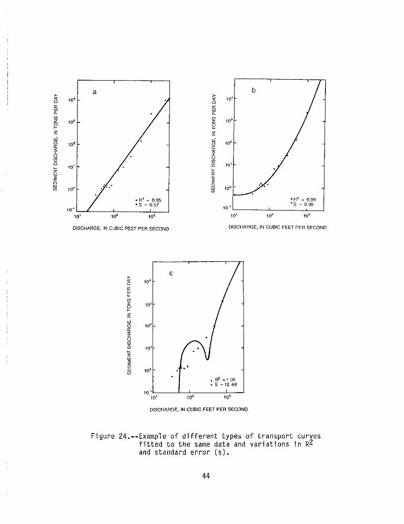
The l a s t problem t o be d iscussed dea ls w i t h t h e tendency t o use t h e s t a t i s t i c s produced by t h e computer f i t t i n g programs t o judge which curve would be t h e b e s t t o use. F igures 24a, b, and c show t h e same da ta as i n f i g u r e 18. The curves show p r o g r e s s i v e l y h i g h e r ~2 va lues w i t h a l l hav ing r e l a t i v e l y low s tandard e r r o r s ( s ) . F i g u r e 24c has a ~ 2 o f 1.00, which would i n d i c a t e a p e r f e c t c o r r e l a t i o n between water and sediment, which i s o b v i o u s l y no t t r u e i n t h i s case, R2 should n o t be used when l o g t rans fo rma- t i o n has been performed on t h e da ta because i t i s no t a measure o f t h e f i t o f t h e da ta b u t o f t h e f i t o f t h e l o g s o f t h e data. Usua l l y t h e bes t cu rve t o use i s t h e s imp les t one which adequate ly represen ts t h e da ta and t h e h y d r o l o g i c c o n d i t i o n s a t t h e s i t e ,

POTENTIAL ERRORS

Es t imates o f sediment d ischarge based on t r a n s p o r t curves a re obv ious l y sub jec t t o e r r o r . The p o t e n t i a l magnitude o f t hose e r r o r s can be demon- s t r a t e d u s i n g t h e da ta shown i n f i g u r e 18. The curve o f a l og -quad ra t i c equa t ion i s f i t t e d t o t h e da ta o f t h e o r i g i n a l s torm ( f i g . 25, same as f i g . 20). I n a d d i t i o n , t h r e e o t h e r storms o c c u r r i n g i n A p r i l , June, and J u l y o f t h e same y e a r a re p l o t t e d . Table 7 shows t h e a c t u a l l oads f o r these storms p l u s t h e es t imated loads based on: ( 1 ) l og -quad ra t i c equat ion, ( 2 ) l o g - l o g equat ion, and ( 3 ) two l o g - l o g equat ions, The percen t o f e r r o r f o r t hese t h r e e s e t s o f t r a n s p o r t curves f o r these f o u r storms ranged f rom 0 t o 1,760 percent .

Table 7.-

Actua l ~ o ~ - ~ u a d r a t i c 1 Log- l og2 Two l og - l og3 measured l oad percent percen t ~ e r c e n t

Storm T/D T/D d i f f e r e n c e T/D d i f f e r e n c e T/D d i f f e r e n c e

O r i g i n a l 2,830 2,330 - 18 1,120 -60 2,830 0 A p r i 1 2,410 1,500 -38 1,330 -45 2,100 -13 June 8,380 156,000 +1 ,760 13,000 +55 33,000 +290 J u 1 y 65 13 -80 18 -72 26 -60

1 ~ n ( ~ ) = 2,624 - 2.567 Ln (x ) + 0.481 Ln (x)**2 ( f i g , 20) 2 ~ n ( y ) = -9.260 + 2.330 L n ( x ) ( f i g . 19) 3Ln(y) = -9.505 + 2.535 Ln (x ) ( r i s i n g s tage and peak) ( f i g . 21)

Ln (y ) = -9.110 + 2.242 Ln (x ) ( r ecess ion ) ( f i g . 21)

DISCHARGE, IN CUBIC FEET PER SECOND DISCHARGE, IN CUBIC FEET PER SECOND


F i g u r e 24.--Examp1 e o f d i f f e r e n t t ypes o f t r a n s p o r t curves f i t t e d t o t h e same da ta and v a r i a t i o n s i n R~ and s tandard e r r o r ( s ) .


F igu re 25.--Examp1 e o f sediment - t r a n s p o r t cu rve ( f i g u r e 20) w i t h da ta f o r a d d i t i o n a l storms added.

I n t h i s case, t h e l o g - l o g t r a n s p o r t cu rve had t h e h i ghes t percen t e r r o r when f i t t e d t o t h e o r i g i n a l da ta (-60 pe rcen t ) b u t gave t h e bes t es t ima te (+55 pe rcen t ) o f t h e ma jo r peak which occur red i n June. Th is may no t always be t r u e , b u t i t has been t h e a u t h o r ' s exper ience t h a t a l o g - l o g o r s e r i e s o f l o g - l o g t r a n s p o r t curves, such as i n f i g u r e s 10, 11, and 15, w i l l no rma l l y g i v e t h e bes t o v e r a l l es t ima te of sediment d ischarge o r concen t ra t ion .

None o f t hese curves p r o v i d e what would be cons idered a "good" es t ima te of sediment load. I n a case such as t h i s example, where l a r g e loops appear i n t h e t r a n s p o r t curve, no s i n g l e l i n e t r a n s p o r t cu rve w i l l g i v e an accura te es t ima te o f sediment t r a n s p o r t . Th i s example aga in i 1 l u s t r a t e s t h e danger o f ex tend ing l og -quad ra t i c t y p e t r a n s p o r t curves beyond t h e da ta used t o d e f i n e them. I n t h i s case, t h e l og -quad ra t i c equa t ion overes t imated t h e June s to rm by 1,760 percent ,

SUMMARY

Sediment- t ranspor t curves a re ve ry u s e f u l when t r y i n g t o es t ima te sed i - ment d ischarge o r concen t ra t i on . Care must be taken i n deve lop ing t hese curves so t h a t e r r o r s i n t h e es t imates a re minimized. Sediment- t ranspor t curves can be drawn based on e i t h e r sediment concen t ra t i on o r sediment d i s - charge vs. water discharge, The u n i t s i n which t h e curve i s drawn shou ld be c o n s i s t e n t w i t h t h e u n i t s t o be est imated,

Care should be t aken t o ensure t h e bes t f i t t o t h e da ta w h i l e n o t v i o l a t i n g any h y d r ~ l o g i c o r hydrau l i c p r i n c i p l e s o f sediment t r a n s p o r t . Seasons, t i m i n g o f sediment peaks vs, water d ischarge peaks, and extreme h i g h sediment events a re j u s t some o f t h e t h i n g s t h a t can a f f e c t t h e s l ope and shape of sed iment - t ranspor t curves, I f computer programs a r e used t o f i t sed iment - t ranspor t curves t o t h e da ta p o i n t s , these curves should be checked f o r t h e i r reasonableness and cons is tency over t h e f u l l range o f water d i s - charges f o r which they w i l l be used. S t a t i s t i c a l parameters should n o t be t h e s o l e c r i t e r i a i n de te rmin ing which cu rve f i t s t h e da ta best, I n any case, thorough a n a l y s i s o f a l l f a c t o r s a f f e c t i n g t h e t r a n s p o r t cu rve must be con- s i de red when deve lop ing and us i ng these curves. Usua l l y t h e bes t cu rve t o use i s t h e s imp les t one t h a t s t i l l de f i nes t h e r e l a t i o n between sediment and wate r discharge.

REFERENCES

Bradu, D., and Mundlak, Y e , 1970, Es t ima t i on i n lognormal l i n e a r models: Journa l o f t h e American S t a t i s t i c a l Assoc ia t ion , v. 65, no. 329, p. 198-211,

Colby, B. R e , 1956, R e l a t i o n o f sediment d ischarge t o s t reamf low: U.S. Geo log ica l Survey Open-Fi l e Report, 170 p.

----- 1964, Discharge o f sands and mean-ve loc i ty r e l a t i o n s h i p s i n sand-bed s t reams: U,S. Geol og i c a l Survey P ro fess i ona l Paper 462-A, 47 p.

C u r t i s , W. F., F l i n t , R e F., and George, F. H:, 1978, F l u v i a l sediment s tudy o f F i s h t r a p and Dewey Lakes d ra inage b a s ~ n s , Ken tucky -V i rg in ia : U.S. Geol og i c a l Survey Open-Fi 1 e Report 77-123, 92 p.

Duan, N., 1983, Smearing est imate: A nonparametr ic r e t r ans fo rma t i on method: Journal o f t h e American S t a t i s t i c a l Assoc ia t ion , v. 78, no. 383, p. 605-610.

Ferguson, R. I., 1986, R i v e r loads underest imated by r a t i n g curves: Water Resources Research, v. 22, no. 1, p. 74-76.

Jones, B. L., and Ewart, C. J., 1973, Hydrology and sediment t r anspo r t , Moanalua Val 1 ey, Oahu, Hawaii : U.S. Geolog ica l Survey, Water Resources D i v i s i o n Report No. HI-HWY-71-1-11, 111 p.

Kno t t , J. M., 1971, Sedimentat ion i n t h e Midd le Fork Eel R i v e r Basin: U.S. Geolog ica l Survey Open-File Report, 60 p.

Koch, R, W., and S m i l l i e , G. M., 1986, B ias i n h y d r o l o g i c p r e d i c t i o n u s i n g log- t ransformed regress ion models: Water Resources B u l l e t i n , v. 22, no. 5, p. 717-723.

P o r t e r f i e l d , George, Busch, R. D., and Waananen, A. O., 1978, Sediment t r a n s p o r t i n t h e Feather R iver , Lake O r o v i l l e t o Yuba City, C a l i f o r n i a : U.S. Geolog ica l Survey Water-Resources I n v e s t i g a t i o n s 78-20, 73 p.

Rantz, S. E., 1968, A no te on r e l a t i n g sediment d ischarge t o stream d ischarge: U.S. Geolog ica l Survey Water-Resources B u l l e t i n , July-September, p. 12-13.

Riggs, H. C., 1968, Some s t a t i s t i c a l t o o l s i n hydro logy: U.S. Geolog ica l Survey Techniques o f Water-Resources I n v e s t i g a t i o n s , Book 4, Chapter A l , 39 p *

Young, L. E., and C r u f f , R. W e , 1967, Magnitude and frequency o f f l o o d s i n t h e Un i t ed States: U.S. Geolog ica l Survey Water-Supply Paper 1686, 308 p.

f? V . 5 . GOVERNMENT P R I N T I N G O F F I C E : 1 9 8 7 - - 1 8 1 - 4 3 8 - - 7 4 1 3 2

4 7

U4HFPBED

Text Box

U4HFPBED

Text Box

U4HFPBED

Text Box

Documents

Glysson, G.D., 1987, Sediment Transport Curves: USGS Open-File