Global Model Analysis by Parameter Space Partitioning

Global Model Analysis by Parameter Space Partitioning

Mark A. Pitt, Woojae Kim, Daniel J. Navarro, and Jay I. MyungOhio State University

To model behavior, scientists need to know how models behave. This means learning what other behaviorsa model can produce besides the one generated by participants in an experiment. This is a difficult problembecause of the complexity of psychological models (e.g., their many parameters) and because the behavioralprecision of models (e.g., interval-scale performance) often mismatches their testable precision in experiments,where qualitative, ordinal predictions are the norm. Parameter space partitioning is a solution that evaluatesmodel performance at a qualitative level. There exists a partition on the model’s parameter space that dividesit into regions that correspond to each data pattern. Three application examples demonstrate its potential andversatility for studying the global behavior of psychological models.

Keywords: model comparison, model complexity, MCMC, connectionist modeling

The experimental method of scientific inquiry has proved towork quite well in psychology. Its unique blend of methodologicalcontrol and statistical inference are effective for testing qualitative(i.e., ordinal) predictions derived from theories of behavior. Datacollection and dissemination have become very efficient, so muchso that far more may be known about a behavioral phenomenonthan is reflected in its corresponding theory.

That our knowledge extends beyond the reach of theory may be asign of productive science and underscores the fact that theories arebroad conceptualizations about behavior that cannot be expected toexplain the minutia in data. Cognitive modeling is a research tool thatcan act as a counterforce to slow and fill this explanatory gap. Itcompensates for a theory’s limitations of precision in data synthesis,description, and prediction. Whether the model is an implementationof an existing theory or a neurally inspired environment in which tostudy processing (e.g., information integration, representational spec-ificity, probabilistic learning), models are rich sources of ideas andinformation on how to think about perception, cognition, and action.The pros and cons of various implementations can be evaluated.Inconsistencies and hidden assumptions can come to light duringmodel creation and evaluation. In short, the modeler is forced toconfront the complexity of what is being modeled and, in the process,can gain insight into the relationship between variables and thefunctionality of the model (see Shiffrin & Nobel, 1998, for a personalaccount of this process).

Of course, the virtues of modeling are accompanied by vices.One of the more serious, often leveled against connectionist mod-

els (Dawson & Shamanski, 1994; McCloskey, 1991) but by nomeans restricted to them, is that model behavior can be mysteriousand difficult to understand, which can defeat the purpose of mod-eling. A model should not be as (or more) complex than the databeing described. Rather, models should offer a simpler and trac-table description.

The preceding observations are not so much a comment aboutmodels or modeling per se but a comment about the need for methodsfor analyzing model behavior. The computational power of cognitivemodels requires correspondingly sophisticated tools to study them.The wide variety of models in the discipline makes the need foruniversal tools all the more pressing and challenging. In this article,we introduce a versatile model analysis and comparison method. Webegin by situating it in relation to existing methods.

Methods of Model Analysis

Model analysis methods can be differentiated along two dimen-sions, whether they measure a model’s local or global behavior,and whether model behavior is evaluated quantitatively or quali-tatively. The position of many analysis methods along these,largely independent, dimensions is shown schematically in Figure1. In the following discussion, quantitative methods are reviewedbefore qualitative ones.

Quantitative Model Analysis

Most quantitative evaluations of models are local. That is, theyconsider the behavior of the model only at its best fitting parametervalues. In contrast, global methods aim to elucidate a model’sbehavior across the full range of its parameter values. Not surpris-ingly, the two approaches are complementary in what they tell usabout model behavior.

Local Quantitative Methods

The most common form of local model analysis is data fitting,in which a model is tested by measuring how closely it approxi-mates (i.e., fits) data generated in an experiment. Because data area reflection of the psychological process under study, a good fit to

Mark A. Pitt, Woojae Kim, Daniel J. Navarro, and Jay I. Myung,Department of Psychology, Ohio State University.

Daniel J. Navarro is now at the Department of Psychology, Universityof Adelaide, South Australia.

This work was supported by Research Grant R01-MH57472 from theNational Institute of Mental Health, National Institutes of Health. Daniel J.Navarro was also supported by a grant from the Office of Research, OhioState University.

Correspondence concerning this article should be addressed to Mark A.Pitt, Department of Psychology, 1885 Neil Avenue, Ohio State University,Columbus, OH 43210-1222. E-mail: [email protected]

Psychological Review Copyright 2006 by the American Psychological Association2006, Vol. 113, No. 1, 57–83 0033-295X/06/$12.00 DOI: 10.1037/0033-295X.113.1.57

57

the data is a necessary condition a model must satisfy to be takenseriously. A good fit determines how well a model passes thesufficiency test of mimicking human performance. It is especiallyuseful in the early stages of model development as a quick andeasy check on sufficiency. Quantitative measures of goodness-of-fit include percentage of variance accounted for, root mean squareddeviation, and maximum likelihood. Although a good fit makes amodel a member of the class of possible contenders, the size of thisclass will depend on the amount and variety of evidence alreadyaccumulated. As more data are collected about an underlyingcognitive process, the number of viable models will diminish. Iftwo models that one is comparing fit all of the data similarly well,other analysis methods are needed to choose between them.

Another local method that is useful for probing model behaviormore deeply than goodness-of-fit is a sensitivity analysis, in whicha model’s parameters are varied around its best fitting values tolearn how robust model behavior is to slight variations of thoseparameters. If a good fit reflects a fundamental property of themodel, then this behavior should be stable across reasonable pa-rameter variation. Another reason a model should satisfy thiscriterion is that human data are noisy. A model should not be sosensitive that its behavior changes noticeably when noise is en-countered. Cross-validation, in which a model is fit to the secondof two data sets using the best fitting parameter values from fittingthe first data set, is a fit-based approach to quantifying this sensi-tivity (Browne, 2000; Stone, 1974).

Global Quantitative Methods

A drawback of local analysis methods is the very fact that theyare local. Each fit provides a view of the model’s behavior at aparticular point in its parameter space but does not provide anyinformation about how it behaves at other parameter settings. Thiscan be particularly disconcerting if the behavior of the model is

sensible only at a few settings. Furthermore, relying on purelylocal methods leaves one with a few snapshots of model perfor-mance that are difficult to piece together into a comprehensiveunderstanding of the model. The task of comparing two models iseven more arduous with local methods.

For these reasons, researchers have begun developing globalanalysis techniques. They are intended to augment local methods,not replace them. From a global perspective, the goal is to learnsomething about the full range of behaviors that a model exhibits.By doing so, we can gain a deeper understanding of the model andhow it compares to competing models. Two of the most popularquantitative global methods are Bayesian methods (e.g., Kass &Raftery, 1995; Myung & Pitt, 1997) and minimum descriptionlength (MDL; e.g., Grunwald, 1998; Grunwald, Myung, & Pitt,2005; Pitt, Myung, & Zhang, 2002; Rissanen, 1996, 2001). In both,the focus is on predictions made by the model at all of its param-eter values. This global perspective yields a natural measure of amodel’s a priori data-fitting potential (i.e., the model’s flexibilityor complexity; Myung, 2000). Although both methods are statis-tically rigorous, technical requirements currently limit their appli-cation to the diverse range of models in psychology.

More recently, Navarro and colleagues (Kim, Navarro, Pitt, &Myung, 2004; Navarro, Pitt, & Myung, 2004; see also Wagen-makers, Ratcliff, Gomez, & Iverson, 2004) introduced a globalquantitative method, called landscaping, that was developed withan eye toward increased versatility and informativeness aboutmodel discriminability. The essence of the technique involvesdetermining how well two models fit each other’s data. What isbeing measured is the extent to which two models mimic oneanother. The approach is attractive as landscapes are relativelyeasy to create, requiring only a comparison of fits to data sets. Inaddition, landscapes can be used to assess the informativeness ofdata in distinguishing pairs of models by inspecting where withinthese landscapes experimental data are located. In short, the land-scape provides a global perspective from which to understand therelationship between two models and their fits to data. However,like MDL and Bayesian methods, landscaping requires that themodels make quantitative predictions. A method free from thisrestriction would have much wider applicability.

Qualitative Methods

Implicit in the use of quantitative methods of model analysis isthat the goal of modeling is to approximate closely empirical data.Although there are good reasons for doing so, one must be carefulto avoid modeling the quantitative minutiae of a data set whilemissing theoretically important qualitative properties or trends inthe data. In the words of Box (1976), “since all models are wrongthe scientist must be alert to what is importantly wrong. It isinappropriate to be concerned about mice when there are tigersabroad” (p. 792). Thus, it is important not to lose sight of quali-tative behavior. In this regard, model evaluation at the qualitativelevel cannot only be informative, but sometimes more appropriate.It is certainly the most common in the psychological sciences.

Hypothesis Testing as a Local Qualitative Method

Hypothesis testing, as used in the experimental method of psy-chological inquiry, is, in essence, a local qualitative method of

Figure 1. The locations of methods of model analysis and comparison ina two-dimensional space, defined by the degree to which the methodevaluates quantitative versus qualitative model performance (vertical axis)and whether the method focuses on local or global model behavior (hori-zontal axis). MDL � minimum description length; SDA � signed differ-ence analysis; PSP � parameter space partitioning.

58 PITT, KIM, NAVARRO, AND MYUNG

model analysis. Hypotheses generated in experimental settings arequalitative predictions about an ordinal pattern of data acrossconditions. One might, for instance, observe a preference reversalunder some experimental conditions that only one of two modelsis able to reproduce. A correct prediction is generally held to bestrong evidence in favor of the winning model and not withoutreason (Platt, 1964). Only in rare circumstances will a modelpredict the exact (interval) quantitative differences among condi-tions. As such, most psychological models are often intended to beillustrative of some underlying process rather than a precise de-scription of its inner workings. Accordingly, the failure of a modelto reproduce the “fine grain” of a data set is not necessarily fatalto the model. It may merely indicate that minor changes arerequired. On the other hand, if a model cannot capture the grossqualitative pattern of the data, something is seriously amiss. Aswith all local methods of model analysis, hypothesis testing is mostinformative when the qualitative pattern in the data can be cap-tured by only one model.

Global Qualitative Methods

Hypothesis testing is the workhorse of model evaluation inmuch of psychology, but like its quantitative counterpart,goodness-of-fit, its focus on local behavior is a limitation. We gainonly a glimpse of what the model can do. It would be useful toknow how many of the other qualitative patterns in that sameexperiment the model could elicit. A model that can produce anylogically possible pattern is no more impressive than one that failsto produce the empirical pattern (Roberts & Pashler, 2000). Inother words, there is the implicit problem pertaining to what wemight call “qualitative complexity or flexibility.” The solution isthe same as with quantitative methods such as MDL: Study thequalitative behavior of the model across a broad range of param-eter values.

Dunn and James’s (2003) signed difference analysis is an ex-ample of global qualitative model analysis. One seeks to identifythe set of signed differences (i.e., pluses or minuses) permittedbetween two data vectors when a model’s parameter values arevaried across the entire parameter space. It is a simple means ofderiving testable ordinal predictions from models in which thefunctional relationship between task performance measurements(e.g., dependent variables) and underlying constructs (i.e., modelparameters) is assumed to be monotonic and otherwise unspeci-fied. This method of global analysis is probably most useful in theearly stages of cognitive modeling where models are definedprimarily in terms of their qualitative predictions and no or fewassumptions are made about other details of the underlying pro-cess. As models become more refined, with elaborate relationshipsbetween dependent variables and model parameters, a more so-phisticated method is needed.

The purpose of the current article is to introduce a highlyinformative method of global qualitative model analysis, param-eter space partitioning (PSP). It involves doing exactly what thename implies: A model’s parameter space is literally partitionedinto regions that correspond to qualitatively different data patternsthat the model could generate in an experiment. Study of theseregions can reveal a great deal about the model and its behavior, aswe show in three application examples. In particular, one can learn

how representative human performance is of the model as well asthe characteristics of other behaviors the model exhibits.

Because the focus of PSP is on qualitative differences in per-formance, the method is more widely applicable than its quantita-tive counterparts such as MDL and Bayesian methods (see Figure1), which are confined to models that can generate probabilitydistributions (e.g., the generalized context model of Nosofsky,1986; the fuzzy logical model of perception [FLMP] of Oden &Massaro, 1978). PSP cannot only be applied to this class of modelsbut to others as well (e.g., connectionist), making it possible tocompare models across classes, a highly desirable feature given thediversity of models in the discipline. The popularity and complex-ity of connectionist models make them an ideal class in which todemonstrate the potential of PSP for studying model behavior.

Parameter Space Partitioning: A GlobalQualitative Method

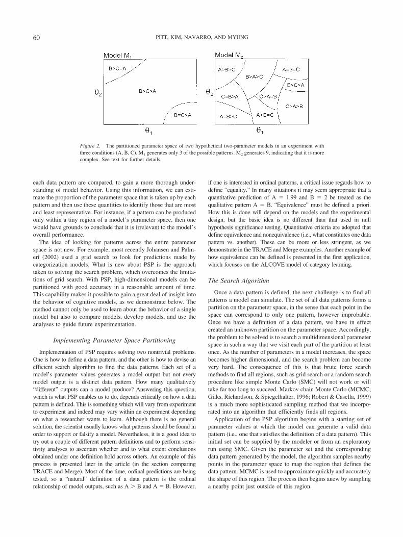
A simple example illustrates the gist of PSP. Consider a visualword recognition experiment in which participants are asked tocategorize stimuli as words or nonwords. The mean response timeto words is then measured as the dependent variable across threeexperimental conditions A, B, and C. In this situation, it may bereasonable to claim that the important theoretical property is theordinal relationship (fastest to slowest) across conditions. In thiscase, there are 13 possible orderings (including equalities) that canbe observed across the three conditions (e.g., A � B � C, A �B � C, B � C � A, etc.). Each of these orderings defines aqualitative data pattern. Suppose further that mean participantperformance yielded the pattern B � C � A.

Now consider two hypothetical models, M1 and M2, of wordrecognition, each with two parameters. Using PSP, we can answerthe following questions about the relationship between the modelsand the empirical data generated in the experiment: How many ofthe 13 data patterns can each model produce? What part of theparameter space includes the empirical pattern? How much of thespace is occupied by the empirical pattern? What data patterns arefound in nearby regions as well as the rest of the parameter space?

Figure 2 shows the parameter space of each model partitionedinto the data patterns it can generate. Model M1 produces threepatterns, one of which is the empirical pattern. Note how it iscentral to model performance, occupying the largest portion of theparameter space. Even though the model generates two otherpatterns, they are smaller and differ only minimally from theempirical pattern. In contrast, M2 produces nine of the 13 patterns.Although one is the empirical pattern, M2’s performance is notimpressive because it can mimic almost any pattern that couldpossibly have been observed in the experiment. Indeed, the factthat M2 can mimic human performance seems almost incidental.Not only does the empirical pattern occupy a small region of theparameter space but larger regions are produced by patterns thatare not human-like (e.g., C � A � B).

As this example illustrates, PSP analyses can be of two types,one focused on the number of patterns and the other on the size ofthe region occupied by a pattern. The goal of the “countinganalysis” is to find and count all of the data patterns that a modelcould potentially generate by varying its parameter values. Whenappropriate, one may also perform a “volume analysis,” in whichthe volumes of the regions in parameter space that are occupied by

59PARAMETER SPACE PARTITIONING

each data pattern are compared, to gain a more thorough under-standing of model behavior. Using this information, we can esti-mate the proportion of the parameter space that is taken up by eachpattern and then use these quantities to identify those that are mostand least representative. For instance, if a pattern can be producedonly within a tiny region of a model’s parameter space, then onewould have grounds to conclude that it is irrelevant to the model’soverall performance.

The idea of looking for patterns across the entire parameterspace is not new. For example, most recently Johansen and Palm-eri (2002) used a grid search to look for predictions made bycategorization models. What is new about PSP is the approachtaken to solving the search problem, which overcomes the limita-tions of grid search. With PSP, high-dimensional models can bepartitioned with good accuracy in a reasonable amount of time.This capability makes it possible to gain a great deal of insight intothe behavior of cognitive models, as we demonstrate below. Themethod cannot only be used to learn about the behavior of a singlemodel but also to compare models, develop models, and use theanalyses to guide future experimentation.

Implementing Parameter Space Partitioning

Implementation of PSP requires solving two nontrivial problems.One is how to define a data pattern, and the other is how to devise anefficient search algorithm to find the data patterns. Each set of amodel’s parameter values generates a model output but not everymodel output is a distinct data pattern. How many qualitatively“different” outputs can a model produce? Answering this question,which is what PSP enables us to do, depends critically on how a datapattern is defined. This is something which will vary from experimentto experiment and indeed may vary within an experiment dependingon what a researcher wants to learn. Although there is no generalsolution, the scientist usually knows what patterns should be found inorder to support or falsify a model. Nevertheless, it is a good idea totry out a couple of different pattern definitions and to perform sensi-tivity analyses to ascertain whether and to what extent conclusionsobtained under one definition hold across others. An example of thisprocess is presented later in the article (in the section comparingTRACE and Merge). Most of the time, ordinal predictions are beingtested, so a “natural” definition of a data pattern is the ordinalrelationship of model outputs, such as A � B and A � B. However,

if one is interested in ordinal patterns, a critical issue regards how todefine “equality.” In many situations it may seem appropriate that aquantitative prediction of A � 1.99 and B � 2 be treated as thequalitative pattern A � B. “Equivalence” must be defined a priori.How this is done will depend on the models and the experimentaldesign, but the basic idea is no different than that used in nullhypothesis significance testing. Quantitative criteria are adopted thatdefine equivalence and nonequivalence (i.e., what constitutes one datapattern vs. another). These can be more or less stringent, as wedemonstrate in the TRACE and Merge examples. Another example ofhow equivalence can be defined is presented in the first application,which focuses on the ALCOVE model of category learning.

The Search Algorithm

Once a data pattern is defined, the next challenge is to find allpatterns a model can simulate. The set of all data patterns forms apartition on the parameter space, in the sense that each point in thespace can correspond to only one pattern, however improbable.Once we have a definition of a data pattern, we have in effectcreated an unknown partition on the parameter space. Accordingly,the problem to be solved is to search a multidimensional parameterspace in such a way that we visit each part of the partition at leastonce. As the number of parameters in a model increases, the spacebecomes higher dimensional, and the search problem can becomevery hard. The consequence of this is that brute force searchmethods to find all regions, such as grid search or a random searchprocedure like simple Monte Carlo (SMC) will not work or willtake far too long to succeed. Markov chain Monte Carlo (MCMC;Gilks, Richardson, & Spiegelhalter, 1996; Robert & Casella, 1999)is a much more sophisticated sampling method that we incorpo-rated into an algorithm that efficiently finds all regions.

Application of the PSP algorithm begins with a starting set ofparameter values at which the model can generate a valid datapattern (i.e., one that satisfies the definition of a data pattern). Thisinitial set can be supplied by the modeler or from an exploratoryrun using SMC. Given the parameter set and the correspondingdata pattern generated by the model, the algorithm samples nearbypoints in the parameter space to map the region that defines thedata pattern. MCMC is used to approximate quickly and accuratelythe shape of this region. The process then begins anew by samplinga nearby point just outside of this region.

Figure 2. The partitioned parameter space of two hypothetical two-parameter models in an experiment withthree conditions (A, B, C). M1 generates only 3 of the possible patterns. M2 generates 9, indicating that it is morecomplex. See text for further details.


Figure 3 illustrates how the algorithm works in the space of atwo-parameter model (see Appendix A for a fuller discussion). Theprocess begins with the initial parameter set serving as the currentpoint in the parameter space (filled point in Panel a). A candidatesample point (shaded point) is drawn from a small, predefinedregion, called a jumping distribution, centered at the current point.The model is then run with the candidate parameter values, and itsoutput is evaluated to determine whether the data pattern is thesame as that generated by the initial point. If so, the candidatepoint is accepted as the next point from which another candidatepoint is drawn. If the new candidate point does not yield the samedata pattern as the initial one, it is rejected as belonging to thecurrent region. Another jump from the initial point is attempted,accepting those points that yield the same data pattern. The se-quence of all accepted points, including repetitions of the samepoint, recorded across all trials is called the Markov chain corre-sponding to the current data pattern. In the language of MCMC,this implementation is called the Metropolis–Hastings algorithmwith a uniform target distribution defined over a given region(Robert & Casella, 1999, ch. 6). As such, the theory of MCMCguarantees that the sample of accepted points will eventually bedistributed uniformly over the entire region. This feature ofMCMC allows us to estimate the volume occupied by the region,regardless of its size (Panel b). A region’s volume is estimatedwith a multidimensional ellipsoid whose shape and size are com-puted using the estimated mean vector and covariance matrix ofthe MCMC sample of the region (see Appendix B for details).

Every rejected point, which must be outside the current region,is checked to see whether it generates a new valid data pattern. Ifso, a new Markov chain corresponding to the newly discoveredpattern is started to define the new region (shaded point in Panelb). In effect, accepted points are used to shift the jumping distri-bution around inside the current region to map it completely,whereas rejected ones are used to initiate new MCMC searchprocesses to map new regions. Over time, as many search pro-cesses as there are unique data patterns will be run. A moreextensive and detailed discussion of the algorithm is provided inAppendix A.

Algorithm Evaluation

We tested the accuracy of the PSP algorithm by measuring itsability to find all of the data patterns defined for a particular model.The difficulty of the search problem was varied by manipulatingthe definition of a pattern (i.e., number of patterns) and the numberof parameters in the model. The extent of both (see Table 1) wasdeliberately made large to make the test challenging. The effi-ciency of the algorithm was measured by comparing its perfor-mance to SMC (random search).

The model was a hypercube whose dimensionality d (i.e., num-ber of parameters) was 5, 10, or 15. To illustrate the evaluationmethod, a two-dimensional model (d � 2) is depicted in Figure 4that contains 20 data regions (outlined in boldface) that the algo-rithm had to find. Note that a large portion of the space does notproduce any valid data patterns. Exactly what constitutes an in-valid pattern will vary across models and experimental setups, butthis area roughly corresponds to those patterns that the model canproduce but do not meet criteria established by the researcher to beconsidered in the analysis. The modeling contexts in which PSP isdemonstrated below provide two very different examples of how adata pattern is defined.

In Figure 4, note that the sizes of the valid data regions vary agreat deal. Some are elicited by a wide range of parameter valueswhereas others can be produced only by a small range of values.This contrast grows exponentially as the dimensionality of themodel increases and was purposefully introduced into the test tomake the search difficult and approximate the complexities (i.e.,nonlinearities) in cognitive models. Ten independent runs of eachsearch method were carried out to assess the reliability of algo-rithm performance.

Figure 5 shows performance of the PSP algorithm for a searchproblem in which there were 100 regions embedded in a 10-dimensional hypercube (d � 10). The PSP algorithm found allregions and did so in 9 minutes. SMC found only about 23 patternsin 9 minutes and, given its sluggish performance, it seems doubtfulthat SMC would find all of them in anything close to a reasonableamount of time.

Table 1 summarizes results from the complete test. The meanproportion of patterns found is listed in each cell. Results are clearand consistent. The PSP algorithm almost always found all of thepatterns, whereas SMC failed to do so in every condition. Mostnoteworthy is the success of the PSP algorithm in the toughestsituation when there were 15 parameters and 500 data patterns. Itsnear perfect success suggests it is likely to perform admirably inother testing situations. (How the current version of the algorithmperforms when regions are not contiguous is discussed in Appen-

Figure 3. Illustrations of two initial steps in the parameter space parti-tioning algorithm. Panel (a) shows the selection of a point (black circle) inthe parameter space and its accompanying jumping distribution (dashedcircle). The shaded circle represents a sample from within the distribution.Panel (b) shows a region in parameter space that the algorithm has mappedout as generating the same data pattern (enclosed area filled with blackdots). The point outside the region (shaded circle), along with a jumpingdistribution, denotes the start of a new search process to map out anotherregion in the parameter space.


dix A, which contains a test of the accuracy of volume estimation.)In the remainder of this article, we describe its applications toanalyzing the behavior of a single model and to comparing designdifferences between two models.

Application 1: Evaluating the QualitativePerformance of ALCOVE

In standard model-fitting analyses, a model’s ability to fit (orsimulate) the data is taken as evidence that it approximates theunderlying cognitive process. In a PSP analysis, the definition offit is relaxed to be a qualitative, ordinal relation on the same scaleas the experimental predictions themselves. Model performance isthen evaluated by determining how many of the possible orderingsof conditions it can produce and how central the empirical pattern

is among them (see Figure 2). In this section, we examined thebehavior of ALCOVE (Kruschke, 1992), a highly successfulexemplar-based account of human category learning in the contextof the seminal Shepard, Hovland, and Jenkins (1961) experiment.Whereas there are some category learning effects that it does notcapture without extension or modification (e.g., Kruschke & Erik-son, 1995; Lee & Navarro, 2002), ALCOVE remains a simple andpowerful account of a broad range of phenomena.

Background to the Analysis

The ALCOVE Model

In some category learning experiments, participants are shown asequence of stimuli, each of which possesses some unknowncategory label. The task is to learn which labels go with whichstimuli, using the feedback provided after responses are made.ALCOVE solves this problem in the following way (for a detaileddescription, see Kruschke, 1992). When stimulus i is presented toALCOVE, its similarity to each of the previously stored exem-plars, sij, is calculated. Following Shepard (1987), similarity isassumed to decay exponentially (with a width parameter c) as afunction of the attention-weighted city-block distance between thetwo stimuli in an appropriate psychological space. After estimatingthese similarities, ALCOVE forms response strengths for each ofthe possible categories. These are calculated using associativeweights maintained between each of the stimuli and the categories.The probability of choosing the kth category follows the choicerule (Luce, 1963) with parameter �.

Having produced probabilities for each of the various possiblecategorization responses, ALCOVE is provided with feedbackfrom an external source. This takes the form of a “humble teacher”vector, in which learning is required only in cases where the wrongresponse was made. Two learning rules are then applied, bothderived by seeking to minimize the sum-squared error between theresponse strengths and the teaching vector, with a simple gradientdescent approach to optimization. Using these rules, ALCOVEupdates the associative weights (with parameter �w for the learning

Figure 4. Illustration of the two-parameter model used to test the param-eter space partitioning algorithm. The algorithm had to find the 20 areasoutlined in bold (valid patterns). The regions outside of this area corre-spond to invalid data patterns. They should be viewed as distractingportions of the parameter space and have the effect of increasing thedifficulty of the search problem.

Figure 5. Search efficiency of the parameter space partitioning (PSP)algorithm compared with simple Monte Carlo (random search). A total of100 patterns had to be found in a 10-parameter model.

Table 1Search Efficiency of the Parameter Space Partitioning (PSP)Algorithm and Simple Monte Carlo (SMC) as a Function of theNumber of Parameters and Data Patterns

No. ofparameters

No. of patterns to find

20 100 500

PSP SMC PSP SMC PSP SMC

5 1.00 0.85 1.00 0.78 1.00 0.8710 1.00 0.32 1.00 0.23 0.99 0.2415 1.00 0.09 1.00 0.02 0.99 0.03

Note. Shown in each cell is the mean proportion of patterns found basedon 10 independent runs.


rate) and the attention weights (with a learning rate parameter �a)prior to observing the next stimulus.

The Shepard, Hovland, and Jenkins (1961) Task

In an experiment, Shepard et al. (1961) studied human perfor-mance in a category learning task involving eight stimuli dividedevenly between two categories. The stimuli were generated byvarying exhaustively three binary dimensions such as color (blackvs. white), size (small vs. large), and shape (square vs. triangle).These authors observed that if these dimensions are regarded asinterchangeable, there are only six possible category structuresacross the stimulus set, illustrated in Figure 6a. This means, forexample, that the category structure that divides all squares intoone category, and all triangles into the other, is regarded asequivalent to the category structure that divides small shapes fromlarge ones, as shown in the lower right.

Empirically, Shepard et al. (1961) found robust differences inthe way in which each of the six fundamental category structureswas learned. In particular, by measuring the mean number of errorsmade by participants in learning each type of category structure,they found that Type I was learned more easily than Type II, whichin turn was learned more easily than Types III, IV, and V (whichall had similar error measures) and that Type VI was the mostdifficult to learn. More recently, Nosofsky, Gluck, Palmeri, Mc-Kinley, and Glauthier (1994) replicated Shepard et al.’s (1961)task with many more participants, and reported detailed informa-tion relating to the learning curves. Figure 6b shows the meanproportion of errors for each category type. Consistent with theconclusions originally drawn by Shepard et al. (1961), it is gen-

erally held that the theoretically important qualitative trend inthese data is the finding that there is a natural ordering on thesecurves, namely that I � II � (III, IV, V) � VI. This kind of patternis called a weak order, as the possibility of ties is allowed.

The psychological importance of this weak order structure issubstantial. Suppose we had two models of the category learningprocess, M1 and M2, of roughly equal complexity. M1 provides areasonably good quantitative fit to the data, by assuming that alltypes are learned at the same rate, and closely approximates theaverage of the six empirical curves. In contrast, M2 reproduces theordering I � II � (III, IV, V) � VI but learns far too slowly and,as a result, fits the data much worse than M1. Since the models areof equivalent complexity, a classical model selection analysiswould prefer model M1. However, while clearly both models havesome flaws, most psychologists would prefer M2, because it cap-tures the theoretically relevant property (i.e., ordinal relationshipamong the six curves) of the data. This discrepancy arises becausequantitative model selection methods like MDL tend to assumethat all properties of the data are equally relevant. In many psy-chological applications, this is not the case. In what follows, weassume that the weak order structure is the important theoreticalproperty of the empirical data and use the PSP method to ask howeffectively ALCOVE captures this structure.

The PSP Analysis

As with any parameterized model, ALCOVE makes differentpredictions at different parameter values. When applied to theShepard et al. (1961) task, ALCOVE will sometimes producecurves that have the same qualitative ordering as the empirical

Figure 6. The Shepard et al. (1961) category types (a), and the learning curves for those types found byNosofsky et al. (1994) in their replication (b). For visual clarity, the curves in Panel b are labeled with arabicnumerals rather than with the more conventional roman numerals. dim � dimensions.


data, but at other times they will look quite different. It would benice to know something about the other orders that ALCOVE canproduce, as it seems that we might learn something about themodel itself. A PSP analysis can provide such information. Usingthe “weak order” definition of a pattern of curves, there are 4,683different data patterns that could possibly be observed in theexperimental task. One would hope that ALCOVE generates onlya small proportion of these and that the extra patterns it doesproduce are interpretable in terms of human performance.

Preliminaries

At this stage, we have only an intuitive definition of a datapattern. However, to perform PSP analyses, one must define aformal method of associating a set of learning curves with aparticular pattern. The weak order that defines a data pattern in theALCOVE example can be decomposed into a set of equivalencerelations and a strong order on the equivalence classes. The strongorder part is easy: We simply rank the classes in terms of meanlearning rate. The equivalence relations are more difficult to de-rive. How does one justify the equivalence of III, IV, and V whenmean learning rate may be similar but not identical? We solved theproblem by relying on a clustering procedure to partition the sixcurves into a natural ordering.

The procedure we used was a variant on the clustering techniqueintroduced by Kontkanen, Myllymaki, Buntine, Rissanen, andTirri (2005). The essence of the technique is to view a clusteringsolution as a probabilistic model for the data. In the currentapplication, the likelihood function for the data takes the form ofa mixture of binomials, with a single multivariate binomial foreach cluster. The clustering procedure now reduces to a statisticalinference problem, which is solved by choosing the set of clustersthat optimizes a minimum description length statistic. The sixlearning curves reported by Nosofsky et al. (1994) are averagedacross 40 participants over the first 16 blocks, consisting of 16stimulus presentations each. Each data point is thus pooled across40 � 16 � 640 trials. Using this technique, it is possible to inferthat I � II � (III, IV, V) � VI is indeed the natural structure forthese data (Navarro & Lee, 2005).

Additionally, we need to be able to associate a set of predictedlearning curves with a data pattern. A set of response probabilitiesis first discretized to the same resolution as the empirical data, byfinding the expected values for the data, given by np, where n isthe sample size and p is the average response probability predictedfor some category type across any given block of trials, and thenrounding to the nearest integer. Although the rounding error is anuisance, it is negligible for n � 640. The discretized curves arethen mapped onto a qualitative data pattern by using the sameclustering technique used to classify the empirical data.

For the PSP analysis of ALCOVE, we constrained the parametervectors (c, �, �w, �a) to lie between (0, 0, 0, 0) and (20, 6, 0.2, 0.2)and disallowed any parameter combination that did not producemonotonic curves. These ranges were deliberately chosen to bequite broad with respect to the kinds of parameter values that aretypically observed in experimental contexts, and nonmonotoniccurves seem highly inappropriate in a simple learning task. In otherwords, the chosen constraints reflect those provided by empiricaldata and by theory.

A technical complication is introduced by the fact that AL-COVE’s predictions are slightly dependent on the order in whichstimuli are observed. Each stimulus has a different effect onALCOVE, so variations in order of presentation produce slightperturbations in the response curves. However, even these minorperturbations can violate the continuity assumptions that underliethe PSP algorithm. In order to deal with these order effects, wechose 20 random stimulus orders and ran the PSP algorithm 10times for each stimulus order, yielding a total of 200 runs. As itturns out, the important properties of ALCOVE appear to beinvariant under stimulus reordering but some unimportant proper-ties are not.

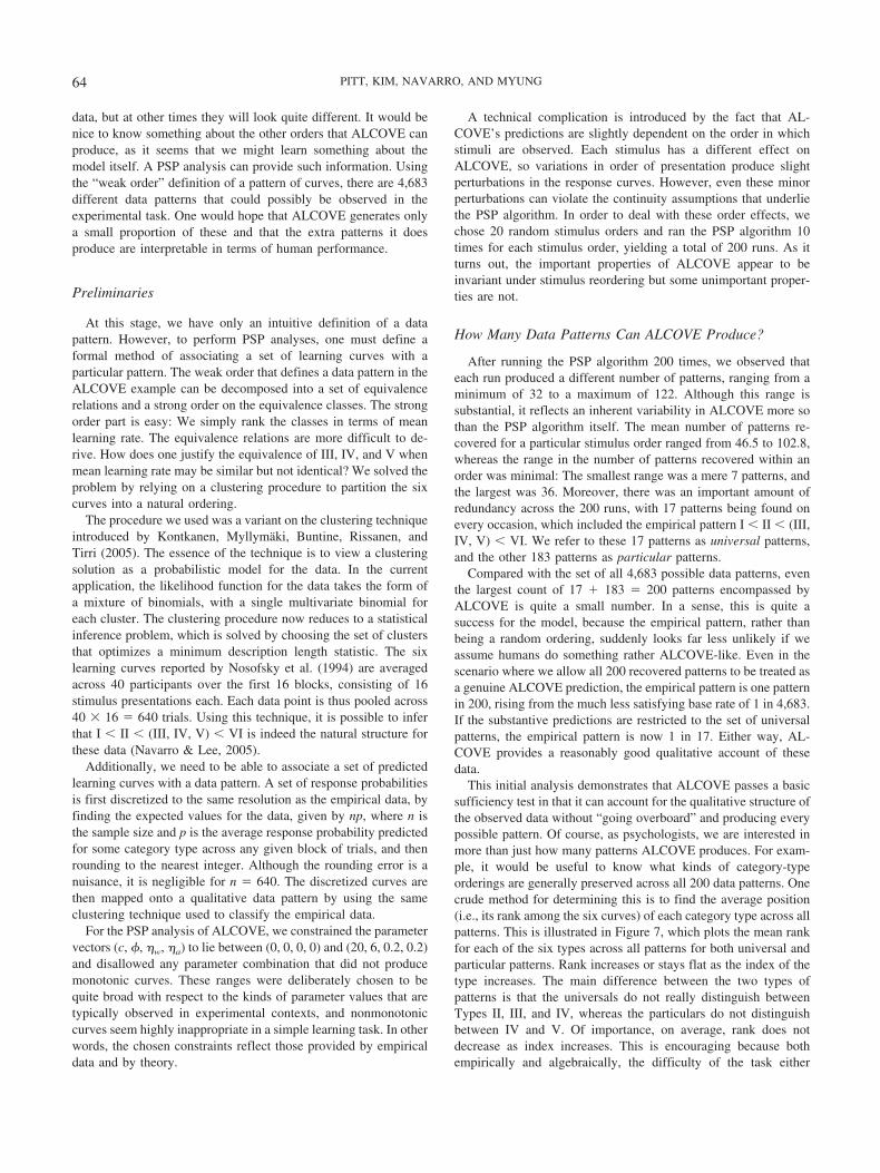
How Many Data Patterns Can ALCOVE Produce?

After running the PSP algorithm 200 times, we observed thateach run produced a different number of patterns, ranging from aminimum of 32 to a maximum of 122. Although this range issubstantial, it reflects an inherent variability in ALCOVE more sothan the PSP algorithm itself. The mean number of patterns re-covered for a particular stimulus order ranged from 46.5 to 102.8,whereas the range in the number of patterns recovered within anorder was minimal: The smallest range was a mere 7 patterns, andthe largest was 36. Moreover, there was an important amount ofredundancy across the 200 runs, with 17 patterns being found onevery occasion, which included the empirical pattern I � II � (III,IV, V) � VI. We refer to these 17 patterns as universal patterns,and the other 183 patterns as particular patterns.

Compared with the set of all 4,683 possible data patterns, eventhe largest count of 17 � 183 � 200 patterns encompassed byALCOVE is quite a small number. In a sense, this is quite asuccess for the model, because the empirical pattern, rather thanbeing a random ordering, suddenly looks far less unlikely if weassume humans do something rather ALCOVE-like. Even in thescenario where we allow all 200 recovered patterns to be treated asa genuine ALCOVE prediction, the empirical pattern is one patternin 200, rising from the much less satisfying base rate of 1 in 4,683.If the substantive predictions are restricted to the set of universalpatterns, the empirical pattern is now 1 in 17. Either way, AL-COVE provides a reasonably good qualitative account of thesedata.

This initial analysis demonstrates that ALCOVE passes a basicsufficiency test in that it can account for the qualitative structure ofthe observed data without “going overboard” and producing everypossible pattern. Of course, as psychologists, we are interested inmore than just how many patterns ALCOVE produces. For exam-ple, it would be useful to know what kinds of category-typeorderings are generally preserved across all 200 data patterns. Onecrude method for determining this is to find the average position(i.e., its rank among the six curves) of each category type across allpatterns. This is illustrated in Figure 7, which plots the mean rankfor each of the six types across all patterns for both universal andparticular patterns. Rank increases or stays flat as the index of thetype increases. The main difference between the two types ofpatterns is that the universals do not really distinguish betweenTypes II, III, and IV, whereas the particulars do not distinguishbetween IV and V. Of importance, on average, rank does notdecrease as index increases. This is encouraging because bothempirically and algebraically, the difficulty of the task either


increases or stays constant as the index increases (see Feldman,2000). This analysis demonstrates that on average, the set of 200patterns that make up ALCOVE’s entire set of qualitative predic-tions roughly preserve an important property of the empirical data:a monotonic increase in learning difficulty across category type.

Which Patterns Matter?

The finding from the preceding counting analysis that somepatterns are frequent (universals) and others rare (particulars)suggests that some may be more representative of model behaviorthan others. However, the frequency with which a pattern is foundis an unsatisfying definition of its importance to a model’s behav-ior, as it confounds the model’s properties with the robustness ofthe search algorithm. This naturally calls for a volume analysis, inwhich the proportion of the parameter space that is occupied byeach pattern is estimated.

Although a model’s parameter space is a potentially importantsource of information about a model, two things must be kept inmind when wanting to distinguish the major patterns that areresponsible for most of ALCOVE’s behavior from the minorpatterns that are irrelevant to the model. The first is that a volumeanalysis is meaningful only if one is willing to ascribe meaning tothe model’s parameters themselves by linking them to psycholog-ical constructs. In the case of ALCOVE, such connections havebeen well motivated (see Kruschke, 1993). Arguably, the nature ofthe exemplar theory on which ALCOVE is based, and the mannerin which the model captures Kruschke’s (1993) “three principles,”provide exactly this kind of justification. The second issue pertainsto the generality of the results. A volume analysis is specific to a

particular parameterization of the model (i.e., how the parametersare defined and combined in the model equation). If the model isreparameterized, the volume analysis could change. In this regard,a volume analysis can draw attention to the appropriateness of amodel’s parameterizations, such as parameter ranges and theirinterdependence.

As it turns out, for ALCOVE there is a strong relationshipbetween the size (i.e., volume) of the region occupied by a patternand the frequency with which it was discovered across the 200runs. In Figure 8, the log of the average volume for each of the 200patterns discovered is plotted against the frequency with whichthey were discovered across the 200 runs of the algorithm. Patternson the far left are the ultimate particulars, having been discoveredonly once, whereas patterns on the far right are the universals,having been discovered on every occasion. Noting that the scale onthe y-axis is logarithmic, we observe that the universals are by farthe largest patterns. The empirical pattern, indicated by the circle,is one of the larger patterns, and is a universal.

The data in Figure 8 allow us to refine our answer to thequestion, “To what extent does ALCOVE predict the empiricalpattern?” The fact that the empirical pattern is among the 17universals is encouraging, as is the regularity in Figure 7. How-ever, by considering the size of the various regions, we can takethis analysis a step further. We could, for instance, exclude allpatterns that do not reach some minimum average size. Thisapproach is illustrated by the horizontal threshold shown in Figure8: Only patterns that occupy more than 1% of the parameter spaceon average lie above this line. This is a pretty stringent test giventhat the parameter space is four-dimensional. Only seven patterns

Figure 7. Means and standard errors for the rank of each category type in the data patterns recovered byparameter space partitioning. The rankings for universals do not differ strongly from the rankings of theparticulars.


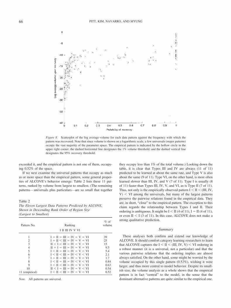
exceeded it, and the empirical pattern is not one of them, occupy-ing 0.52% of the space.

If we next examine the universal patterns that occupy as muchas or more space than the empirical pattern, some general proper-ties of ALCOVE’s behavior emerge. Table 2 lists these 11 pat-terns, ranked by volume from largest to smallest. (The remainingpatterns—universals plus particulars—are so small that together

they occupy less than 1% of the total volume.) Looking down thetable, it is clear that Types III and IV are always (11 of 11)predicted to be learned at about the same rate, and Type V is alsoabout the same (9 of 11). Type VI, on the other hand, is most oftenlearned slower than III, IV, and V (7 of 11). Type I is usually (8of 11) faster than Types III, IV, V, and VI, as is Type II (7 of 11).Thus, not only is the empirically observed pattern I � II � (III, IV,V) � VI among the universals, but many of the largest patternspreserve the pairwise relations found in the empirical data. Theyare, in short, “close” to the empirical pattern. The exception to thisclaim regards the relationship between Types I and II. Theirordering is ambiguous. It might be I � II (4 of 11), I � II (4 of 11),or even II � I (3 of 11). In this case, ALCOVE does not make astrong qualitative prediction.

Summary

These analyses both confirm and extend our knowledge ofALCOVE. It should comfort category learning researchers to learnthat ALCOVE captures the I � II � (III, IV, V) � VI ordering ina robust manner (it is a universal, not a particular) and that thevarious pairwise relations that the ordering implies are almostalways satisfied. On the other hand, some might be worried by thevolume occupied by this single pattern (0.52%), wishing it werelarger, and thus more central to model behavior. Despite its small-ish size, the volume analysis as a whole shows that the empiricalpattern is in fact “central” to the model, in the sense that thedominant alternative patterns are quite similar to the empirical one.

Figure 8. Scatterplot of the log average-volume for each data pattern against the frequency with which thepattern was recovered. Note that since volume is shown on a logarithmic scale, a few universals (major patterns)occupy the vast majority of the parameter space. The empirical pattern is indicated by the hollow circle in theupper right corner; the dashed horizontal line designates the 1% volume threshold; and the dashed vertical linedesignates the 95% recovery threshold.

Table 2The Eleven Largest Data Patterns Predicted by ALCOVE,Shown in Descending Rank Order of Region Size(Largest to Smallest)

Pattern No. Ranking% of

volume

I II III IV V VI

1 I � II � III � IV � V � VI 392 I � II � III � IV � V � VI 253 II � I � III � IV � V � VI 154 II � I � III � IV � V � VI 9.55 I � II � III � IV � V � VI 5.46 I � II � III � IV � V � VI 2.17 I � II � III � IV � V � VI 1.78 I � II � III � IV � V � VI 0.849 I � II � III � IV � V � VI 0.63

10 II � I � III � IV � V � VI 0.5411 (empirical) I � II � III � IV � V � VI 0.52

Note. All patterns are universal.


“Distant” patterns (i.e., violations of weak orderings) are rarely ifever generated by ALCOVE; this information is very useful toknow in model evaluation. In this regard, the added understandingprovided by this global analysis of ALCOVE increases one’sconfidence in claiming that the model can “account” for the dataprecisely because we know the range of behaviors it exhibits inthis experimental setting.

The PSP analysis also revealed some unexpected behaviors. It issomewhat surprising that it is even possible for ALCOVE topredict II � I. It may be that this happens only with very oddchoices of parameters (i.e., ones that are computationally feasiblebut psychologically bizarre) and is certainly something that wouldbe interesting to explore in future work.

Application 2: Comparing the Architecturesof Merge and TRACE

In addition to learning about the behavior of a single model, PSPanalyses can inform us about the behavioral consequences ofdesign differences between models. In this and the next example,PSP is applied to two localist connectionist models of speechperception, TRACE (McClelland & Elman, 1986) and Merge(Norris, McQueen, & Cutler, 2000). We compared them in twoexperimental settings, one intended to bring out architectural dif-ferences and the other differences in weighting bottom-up (sen-sory) information.


Architectural Differences of TRACE and Merge

The two models are illustrated schematically in Figure 9. Theyare similar in many ways. Both have a phonemic input stage anda word stage. There are excitatory connections from the phonemeinput to the word stage and inhibitory connections within the wordstage. They differ in how prior knowledge is combined withphonemic input to yield a phonemic decision (percept). In

TRACE, word (prior) knowledge can directly affect sensory pro-cessing of phonemes. This is represented by direct excitatoryconnections from the word stage back down to the phoneme stage.Also note that in TRACE the phoneme stage performs double duty,also serving as a phoneme decision stage. In Merge, these twoduties are purposefully separated into two distinct stages to preventword information from affecting perceptual processing of pho-nemes. Instead, lexical knowledge affects phoneme identificationvia excitatory connections from the word to the phoneme decisionstage. In contrast to the direct interaction between phoneme andword levels in TRACE, these two sources of information areintegrated at a later decision stage in Merge.

Although not visible in the diagrams in Figure 9, the modelsdiffer in another important way. In keeping with the belief thatbottom-up (sensory) information takes priority in guiding percep-tion early in processing, activation of a phoneme decision node inMerge must be initiated by phoneme input before excitatory lex-ical activation can affect phoneme decision making. TRACE con-tains no such constraint.

The goal of our investigations was to assess the impact of thesetwo design differences on global model behavior. Norris et al.(2000) proposed Merge as an alternative to TRACE because theyfelt that the evidence from the experimental literature did notwarrant interaction (i.e., direct word-to-phoneme feedback). Theadequacy of the Merge architecture was demonstrated in simula-tion tests in which it performed just as well as, if not slightly betterthan, TRACE in reproducing key experimental findings. PSPanalyses of the models’ behaviors were performed in two of theseexperimental settings. In the first, the subcategorical mismatchstudy by Marslen-Wilson and Warren (1994), the consequences ofsplitting phoneme processing into separate input and decisionstages, was evaluated. In the second, the indirect inhibition exper-iment of Frauenfelder, Segui, and Dijkstra (1990), the contributionof the bottom-up priority rule to model performance, wasexamined.

Figure 9. Schematic diagrams of TRACE and Merge.


In order to compare the two models, it was necessary to equatethem on all nonessential dimensions (e.g., size of lexicon) toensure that differences in performance were attributable only todesign differences (e.g., connectivity, number of parameters). Inessence, we wanted to compare the fundamental structural andfunctional properties that define the models. We did this by firstimplementing the version of Merge described in Norris et al.(2000), and then making the necessary changes to Merge to turn itinto TRACE. In the end, TRACE required four fewer parametersthan MERGE. The names of the parameters, along with othermodel details, are provided in Appendix C.

The Subcategorical Mismatch Experiment

The first comparison of the two models was performed in thecontext of the subcategorical mismatch experiment of Marslen-Wilson and Warren (1994, Experiment 1; McQueen, Norris, &Cutler, 1999, Experiment 3). The setup is attractive because of thelarge number of conditions and response alternatives, which to-gether permitted detailed analyses of model behavior at both thephonemic and lexical levels. In the experiment, listeners heardone-syllable utterances and then had to classify them as words ornonwords (lexical-decision task) or categorize the final phoneme(phonemic decision task). The stimuli were made by appending aphoneme (e.g., /b/ or /z/) that was excised from the end of a word(e.g., job) or nonword (e.g., joz) to three preceding contexts, toyield six experimental conditions (listed in Table 3). The firstcontext was a new token of those same items but with the finalconsonant removed (e.g., jo), to create cross-spliced versions ofjob and joz. The second consisted of equivalent stretches of speechfrom a word that differed only in the final consonant (e.g., jo fromjog in both cases). The third was the same as the second except thatthe initial parts were excised from two nonwords (e.g., jo from jodand jo from jov).

Because cues to phoneme identity overlap in time (because ofcoarticulation in speech), a consequence of cross-splicing is thatcues to the identity of the final consonant will conflict when thefirst word ends in a consonant different from the second. Forexample, jo from jog contains cues to /g/ at the end of the vowel,which will be present in the resulting stimulus when combinedwith the /b/ from job (Condition 2 in Table 3).

Marslen-Wilson and Warren (1994) were interested in how suchstimuli affect phoneme and lexical processing. As the results inTable 3 show (taken from McQueen et al., 1999), in the lexicaldecision task, reaction times slowed when listeners heard cross-spliced stimuli, but responding was not affected by the source ofthe conflicting cues (i.e., equivalent RTs in Conditions 2 and 3).Phoneme categorization, in contrast, was sensitive to the subtlevariation in phonetic detail, but only when the stimulus itselfformed a nonword (e.g., joz; Conditions 5 and 6). Notably, the useof cross-spliced stimuli nullifies the bottom-up priority rule inMerge, which otherwise might have contributed to any differences(see Norris et al., 2000, for details). To the extent that differencesare found across models, they are probably a result of theirdifferent architectures.

The Parameter Space Partitioning Analysis

The subcategorical mismatch experiment contains two depen-dent measures of performance, classification decisions and thespeed with which those decision were made (response time). Wetreated classification performance as a qualitative pattern in thePSP analysis. We then performed a separate investigation of theRT predictions.

Preliminaries

Classification in these two models is usually defined in terms ofthe activation state of the network when specific decision criteriaare met, such as a phoneme node exceeding an activation thresh-old. Because there are multiple conditions in the subcategoricalmismatch experiment, a data pattern is really a profile of classifi-cations across these conditions. In this experiment there are sixconditions, with a phoneme and lexical response in each, for a totalof 12 categorization responses that together yield a single datapattern. With four possible phoneme responses and three possiblelexical responses, there were a total of 2,985,984 (46 � 36)patterns. Of interest is how many and which of these patternsTRACE and Merge produce.

We applied two classification decision rules. The effect of theserules is that they establish the necessary mapping between thecontinuous space of network states to the discrete space of data

Table 3Design of the Subcategorical Mismatch Simulation in Norris, McQueen, and Cutler (2000)

Condition ExamplePhonemic

categorization Lexical decision Phonemic categorization Lexical decision

Word /b/ /g/ /z/ /v/ ‘job’ ‘jog’ nonwordMatching cues job�job 668 340 � �Mismatching cues from word jog�job 804 478 � �Mismatching cues from nonword jov�job 802 470 � �

Nonword /b/ /g/ /z/ /v/ ‘job’ ‘jog’ nonwordMatching cues joz�joz 706 NA � �Mismatching cues from word jog�joz 821 NA � �Mismatching cues from nonword jov�joz 794 NA � �

Note. Underlined segments denote the sections of the utterances that were excised and then combined. The condition names describe whether the cuesto the final consonant in the first word matched those of the second word. Reaction time data are from McQueen et al (1999). Response sets in each taskin the simulations are shown at the right. Check marks denote listeners’ dominant response. NA � not applicable.


patterns, making it possible to associate each data pattern with aregion in parameter space. Because any one rule could yield adistorted view of model performance, the use of two rules enabledus to assess the generality of the results. In addition, we found thatsome model properties that are not evident with one criterionemerged when performance was compared across rules. The firstrule, labeled weak threshold, was a fixed activation threshold, withvalues of 0.4 for phoneme nodes and 0.2 for lexical nodes. It is thesame rule used by Norris et al. (2000) and was adopted to maintaincontinuity across studies.

The second rule, called the stringent threshold, required classi-fication to be more decisive, by requiring the activation level ofcompeting nodes to be significantly lower than the winning node.Two thresholds were used, the higher of which was the lowerbound for the chosen node and the lower of which was the upperbound for the nearest competitor. These values were 0.45 and 0.25for phoneme classification and 0.25 and 0.15 for lexical decision.Two other constraints were also enforced as part of the stringentthreshold. There had to be a minimum difference in activationbetween the winning node and its closest competitor of 0.3 forphoneme classification and 0.15 for lexical decision. Finally, fornonword responses in lexical decision, the difference in activationbetween the two lexical items, jog and job, could not be more than0.1.

The models were designed as depicted in Figure 9. The onlylexical nodes were job and jog. All necessary phoneme nodes wereincluded, with /b/, /z/, /g/, /v/ being of primary interest. The PSPalgorithm was run for both models and both decision rules. Toobtain a data pattern, all six stimuli were fed into the model, andboth phoneme and lexical classification responses assessed. Thealgorithm and models were run in Matlab on a Pentium IV com-puter. The time required to find all patterns varied greatly, takingas little as 22 min (TRACE, stringent threshold) and as long as 24hr (Merge, stringent threshold). The consistency of results wasascertained using five multiple runs for each model and threshold.The averaged data are presented below.

How Many Patterns Do the Models Produce?

The analysis began by comparing classification (asymptotic)performance of the two models. Table 4 contains three measuresthat define their relationship under the weak and stringent thresh-olds. The second column contains Venn diagrams that depict thesimilarity relation between the models when measured in terms ofthe number of data patterns each can generate. Looking first at theweak threshold data, both models generate 21 common patterns,with TRACE producing only a few unique patterns compared withMerge (2 vs. 30). The filled dot represents the empirical pattern,which both models produced.

The nature of the overlap in the diagram indicates that TRACEis virtually nested within Merge, with 21 of its 23 patterns alsobeing ones that Merge produces. However, Merge can produce anextra 30 patterns, suggesting that in the subcategorical mismatchdesign, Merge is more flexible (i.e., complex) than TRACE.1 Thatsaid, the difference between them is not all that great, although itdoes not disappear under further scrutiny (see below). Perhapsmost impressively, both models are highly constrained in theirperformance, generating fewer than 60 of the some 3 millionpatterns that are possible in the design.

When the stringent threshold is imposed, both models generatefewer patterns, with TRACE producing 7 and Merge 26, as indi-cated in the lower half of Table 4. Nevertheless, the relationshipbetween the models remains unchanged: TRACE is almost nestedwithin Merge. However, the one unique TRACE pattern turns outto be the empirical data, which Merge no longer generates.

Notably, the change in threshold primarily caused a drop in thenumber of shared patterns, indicating that the models are moredistinct under the stringent threshold. This can be understood byturning one’s attention to columns 3 and 4, which contain esti-mates of the proportion of the parameter space occupied by thevalid data patterns. Although the percentages for both models israther small, half as much of TRACE’s parameter space is usedcompared with Merge’s. Predictably, the regions shrink when thestringent threshold is applied. If one then examines how much ofeach valid volume is occupied by common and unique patterns, thereason for the increased distinctiveness of the models presentsitself. For TRACE (column 5), this region is occupied almostentirely by the 21 common patterns (100%). Under the stringentthreshold, this value drops slightly to 92%, but because there isonly one unique pattern in this case, its value must be 8%, the sizeof the region occupied by the empirical pattern. The remaining 15common patterns (21 – 6) occupied such tiny regions in TRACE’sparameter space under the weak threshold that application of thestringent threshold eliminated them. A similar situation occurredwith Merge (column 6), with 12 of the 16 common patterns (ofwhich the empirical pattern was one) disappearing as a result of achange in threshold. Four became unique to Merge. A few patternsunique to each model also failed to satisfy the stringent threshold(2 for TRACE and 7 for Merge).

1 Indeed, equating the number of patterns with model complexity is anatural and well-justified definition of complexity (Myung, Balasubrama-nian, & Pitt, 2000).

Table 4Classification Results From the Subcategorical Mismatch Test


Although a change in threshold brings out differences in themodels, analysis of their common patterns under both thresholdsreveals an impressive degree of similarity. For example, under theweak threshold, the regions in parameter space of all 21 patternsare comparable in size across models. To measure this, we corre-lated the rank orderings (from smallest to largest) of the volumesin the two models. Use of the actual volume estimates themselvesis inappropriate because of differences in model structure andparameterization. With � � .75, the correlation is high. For thestringent threshold it is slightly lower, � � .60, but keep in mindthat there were only six data points in this analysis. These associ-ations indicate that the overlap between models is not just nominalin terms of shared data patterns, but those regions are similar inrelative size with all other common regions, making the modelsfunctionally highly similar.

Is the Variation Across Patterns Sensible?

To the extent that a model produces data patterns other than theempirical one, a mark of a good model is for its performance todegrade gracefully. In the first application of PSP, ALCOVE’sperformance degraded gracefully because all of its patterns lookedsimilar to the empirical one. In the current analysis, we measureddeviation by counting the number of mismatches (different deci-sions) between a particular pattern and the empirical one. Becausea pattern consists of 12 decisions, there are a maximum of 12possible mismatches (6 phonemic and 6 lexical). Histograms of themismatch counts were created for both models and are shown inFigure 10 alongside a histogram showing the base rate at eachmismatch distance (e.g., there are thousands of possible patternswith six mismatches, but only 12 patterns with one mismatch).

Both models show a remarkable proclivity to produce human-like data. The distributions are located near the zero endpoint(empirical pattern) with peaks between two and four mismatches.The probability is virtually zero that a random model (i.e., arandom sample of patterns) would display such a low mismatchfrequency. The weak threshold distributions are slightly to theright of the stringent threshold distributions, and Merge’s distri-butions are slightly to the right of TRACE’s. In both cases, this isprobably a base rate effect; allowing more patterns increases thelikelihood of more mismatches.2

An equally desirable property of a model is that patterns thatmismatch across many conditions occupy a much smaller region inthe parameter space than those that mismatch by only one or twoconditions. That is, larger regions should correspond to patternsthat are more similar to the empirical pattern. When region volumeis correlated with mismatch distance, this is generally true for bothmodels but stronger for Merge (� � �0.51) than TRACE (� ��0.38).

The mismatch distributions beg the question, What types ofclassification errors do the models make? To answer this, theproportion of mismatches in each of the 12 conditions was com-puted for each model, and these are plotted in Figure 11. Theprofile of mismatches across conditions again reveals more simi-larities than differences between the models. For the most part themodels performed similarly. The only noteworthy differences arethat Merge produced more phoneme misclassifications (Condi-tions 3 and 6), and TRACE produced a greater proportion oflexical misclassifications. In the four phoneme conditions in whicherrors were made, the final phoneme was created by cross-splicing

two different phonemes, creating input that specified one weaklyand the other strongly. The errors are a result of misclassifying thephoneme as the more weakly specified (lowercase) alternative(e.g., g instead of B). By design, Merge’s bottom-up only archi-tecture heightens its sensitivity to sensory information, which inthe present simulation made it a bit more likely than TRACE tomisclassify cross-spliced phonemes.

Lexical misclassification errors in TRACE are due primarily toa bias to respond “nonword.” However, a small percentage of theselexical errors were due to classifying the stimulus as jog (Condi-tion 5). This also occurred in Condition 2, but much less often,with misclassifications as jog constituting 8% of the mismatchesfor TRACE and 3% for Merge.

Which Patterns Matter?

Although some misclassifications can be legitimized on manygrounds (e.g., humans make such errors, perception of ambiguousstimuli will not be constant), it is important to determine whetherthey are characteristic behaviors of the model or idiosyncraticpatterns, such as the “particulars” defined in the ALCOVE anal-ysis. That is, it is useful to distinguish between unrepresentativeand representative behaviors. To do so, we measured the volumesof all regions identified by the PSP algorithm. Recall that absolutevolume estimates are not compared directly, but rather relative tothe total volume of the valid regions of the model, as ratios(percentages). This step is essential because it makes it possible tocompare volume estimates of equivalent regions (same data pat-tern) between models. The size of a region occupied by a datapattern is normalized by the total volume of each model, placingthem on an equal footing. Differences in volume must therefore be

2 Subsequent analyses in this section are restricted to the weak-thresholddata, in part because of the paucity of common patterns. General conclu-sions do not change.

Figure 10. Similarity of all Merge and TRACE data patterns to theempirical (human) pattern measured in terms of the number of mismatchesto the empirical pattern. Data from the application of the weak andstringent thresholds are shown separately. The dashed line represents thedistribution of mismatches for all patterns in the experimental design.


attributable to differences in model behavior, whether it is some-thing as simple as parameter range differences or something morefundamental, such as how the parameters are combined.

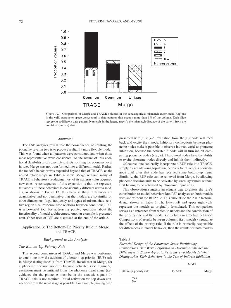
As in the ALCOVE analysis, a threshold of 1% of the validvolume was adopted to define a meaningful pattern. When this isdone, many patterns turn out to be noise and the set of represen-tative patterns is reduced to a handful. For TRACE, 21 of itspatterns (2 unique and 18 common) do not meet this criterion. Fourpatterns, all common, dominate in volume, together accounting for99% of the volume (range � 4.1% to 57.9%). For Merge, the setof dominant patterns is larger and is split equally between commonand unique patterns. Thirty-six patterns (21 unique and 15 com-mon) fail to reach the 1% criterion. Seven common (range � 2.0%to 27.6%) and eight unique (range � 1.4% to 21.1%) patterns doso and make up 97% of the valid volume. Even with a thresholdthat eliminated 75% of all patterns, the asymmetry in patterngeneration between the models is still present (TRACE � 4;Merge � 15).

The volumes of these representative common patterns aregraphed in Figure 12. The numerals in the legend refer to themismatch distance of each common pattern from the empiricalpattern. Most obvious is the fact that the empirical pattern is muchlarger in TRACE than in Merge (27% and 6.8%) and that onemismatching pattern (filled black) dominates in both models(57.9% and 27.6%). This pattern turns out to be one in which thereis a bias to classify all stimuli as nonwords. As a group, the eightunique Merge patterns mismatch the empirical pattern more thanthe common patterns. The largest pattern occupies a region of21.1% (five mismatches), more than twice the next largest region(8.4%). In this pattern, not only did Merge exhibit the samenonword response bias, but it also categorized cross-spliced pho-nemes as the competing (remnant) phoneme.

Response Time Analyses

Up to this point in the analysis we have compared only theclassification behavior of the models, but the time course ofprocessing is equally important, as experimental predictionsoften hinge on differences in RT between conditions. TRACEand Merge are often evaluated on their ability to classify stimuliat a rate (e.g., number of cycles) that maintains the same ordinalrelations across conditions found with RTs. To assess the ro-bustness of simulation performance, parameters can be variedslightly and additional simulations then run to ensure thatthe model does not violate this ordering (e.g., by producinga change in the RT pattern). In their comparison of Mergeand TRACE, Norris et al. (2000) found that neither pro-duced an RT reversal. Our test was a more exhaustive versionof theirs.

The PSP analysis defines for us the region in the parameterspace of each model that corresponds to the empirical datapattern. When assessing RT performance, what we want toknow is whether there are any points (i.e., parameter sets) inthis region that yield invalid RT patterns, as defined by theordinal relations among conditions in the experiment (i.e., theRT pattern in the six phonemic and three lexical conditions inTable 3). To perform this analysis, 10,000 points were sampledover the uniform distribution of the empirical region. Simula-tions were then run with each sample, and the cycle time atwhich classification occurred was measured and comparedacross all conditions. Violations were defined as reversals incycle times between adjacent conditions (e.g., Condition 1 vs.Condition 2) in phoneme classification and lexical decision.Just as Norris et al. (2000) reported, we did not find a singlereversal between conditions for either model.

Figure 11. Proportion of mismatches by Merge and TRACE across the 12 conditions. The two-letter sequencesare shorthand descriptions of the cross-spliced stimuli used in the conditions. The lowercase letter denotes thefinal phoneme of the first word, and the uppercase letter denotes the final phoneme of the second word.


Summary

The PSP analyses reveal that the consequence of splitting thephoneme level in two is to produce a slightly more flexible model.This was found when all patterns were considered and when thosemost representative were considered, so the nature of this addi-tional flexibility is of some interest. By splitting the phoneme levelin two, Merge was not transformed into a different model. Rather,the model’s behavior was expanded beyond that of TRACE, as thenested relationships in Table 4 show. Merge retained many ofTRACE’s behaviors (producing most of its patterns) plus acquirednew ones. A consequence of this expansion is that the represen-tativeness of these behaviors is considerably different across mod-els, as shown in Figure 12. It is because these differences arequantitative and not qualitative that the models are so similar onother dimensions (e.g., frequency and types of mismatches, rela-tive region size, response time relations between conditions). PSPis a powerful tool for addressing pointed questions about thefunctionality of model architectures. Another example is presentednext. Other uses of PSP are discussed at the end of the article.

Application 3: The Bottom-Up Priority Rule in Mergeand TRACE


The Bottom-Up Priority Rule

This second comparison of TRACE and Merge was performedto determine how the addition of a bottom-up priority (BUP) rulein Merge distinguishes it from TRACE. Recall that in Merge, fora phoneme decision node to become activated (see Figure 9),excitation must be initiated from the phoneme input stage (i.e.,evidence for the phoneme must be in the acoustic signal). InTRACE, this is not required. Initial activation via top-down con-nections from the word stage is possible. For example, having been

presented with jo in job, excitation from the job node will feedback and excite the b node. Inhibitory connections between pho-neme nodes make it possible to observe indirect word-to-phonemeinhibition, because the activated b node will in turn inhibit com-peting phoneme nodes (e.g., g). Thus, word nodes have the abilityto excite phoneme nodes directly and inhibit them indirectly.

Of course, one can easily incorporate a BUP rule into TRACE,simply by not allowing top-down feedback to influence a phonemenode until after that node has received some bottom-up input.Similarly, the BUP rule can be removed from Merge, by allowingphoneme decision units to be activated by word layer units withoutfirst having to be activated by phonemic input units.

This observation suggests an elegant way to assess the rule’scontribution to model behavior: Run PSP analyses on both modelswith and without the BUP rule. This amounts to the 2 � 2 factorialdesign shown in Table 5. The lower left and upper right cellsrepresent the models as originally formulated. This comparisonserves as a reference from which to understand the contribution ofthe priority rule and the model’s structures in affecting behavior.Comparisons of results between columns (i.e., models) neutralizethe effects of the priority rule. If the rule is primarily responsiblefor differences in model behavior, then the results for both models

Figure 12. Comparison of Merge and TRACE volumes in the subcategorical mismatch experiment. Regionsin the valid parameter space correspond to data patterns that occupy more than 1% of the volume. Each slicerepresents a different data pattern. Numerals in the legend specify the mismatch distance of the pattern from theempirical (human) data.

Table 5Factorial Design of the Parameter Space PartitioningComparisons That Were Performed to Determine Whether theDifferences in Bottom-Up Priority in the Two Models Is WhatDistinguishes Their Behaviors in the Test of Indirect Inhibition

Bottom-up priority rule

Model

TRACE Merge

YesNo


should be quite similar when the rule is and is not operational. Ifdifferences still remain, then structural differences are also con-tributing to their diverse behaviors. In short, these analyses will tellus whether Merge, without its priority rule, behaves like TRACE,and whether TRACE, with the priority rule, mimics MERGE.

The Frauenfelder et al. (1990) Data

If indirect word-to-phoneme activation is possible, then onewould expect anomalous word endings to slow down responses tothose endings. Frauenfelder et al. (1990, Experiment 3) tested thisprediction by having listeners monitor for phonemes that occurredlate in multisyllabic words and nonwords. Three conditions are ofinterest in the present analysis. A word condition (e.g., habit, with/t/ as the target phoneme) served as a lower bound on respondingbecause lexical and phonemic information should combine to yieldfast RTs. A control nonword condition (e.g., mabil, with /l/ as thetarget phoneme) served as a reference against which to measureinhibition. Because mabil is not a word, there should be notop-down lexical facilitation or inhibition when responding to /l/;responses should be based on sensory input alone. In the third,inhibitory condition, listeners heard nonwords such as habil, withl as the target phoneme. A slowdown in RT relative to the controlnonword condition is expected if there is in fact inhibition. This isbecause the first part of the stimulus, habi, will excite habit, whoseactivation should then feed back down and excite /t/, which willthen inhibit /l/.

The RT slowdown in the inhibition condition was small and notreliable despite significant effects in companion conditions andexperiments. That this seemingly clear prediction of TRACE wasnot borne out in the data has generally been interpreted as arguingagainst word-to-phoneme excitation in TRACE. However, in sim-ulations of indirect inhibition, TRACE’s behavior is not cut anddry, with inhibition being more likely with longer than shorterwords (Norris et al., 2000). In contrast, the BUP rule in Mergeguarantees that it produces consistent performance that neveryields inhibition. TRACE’s variable behavior is a sign that it cangenerate more data patterns than Merge. If this is the case, is theabsence of the priority rule the main cause, or is it also due tostructural differences between the models?

The Parameter Space Partitioning Analysis

Preliminaries

The design of the indirect inhibition experiment is much simplerthan the subcategorical mismatch experiment. There are only threeconditions and only a single response (phonemic decision). Tosimulate the experiment, the combination of so few conditions anda simple model design (one lexical and two critical phonemenodes) would yield so few potential data patterns that the analysismight not provide satisfying answers to our question. We thereforeadded a lexical decision response (word or nonword) to the designon the grounds that listeners would, if asked, accurately categorizeeach stimulus as a word or nonword. The models should performsimilarly. This additional response permitted a more fine-grainedanalysis and comparison of the models.

Input to the models consisted of three utterances: habit, mabil,habil. They were selected to be moderately long (five phonemes)so that indirect inhibition would have a chance to emerge. Both

models were modified from the previous test to consist of only onelexical node (habit) and the appropriate phoneme input/decisionnodes, with /t/ and /l/ of most interest because their activationfunctions were used to test for inhibition. With two classificationresponses, each with two alternatives, and three stimulus condi-tions, there were a total of 64 possible data patterns (23 � 23).

To examine the effect of the BUP rule on model performance,we adjusted phoneme activation parameters accordingly in eachmodel prior to running the PSP algorithm. The same two decisionrules were again used to assess the generality of results. With twodecision rules and two priority rules, the algorithm was run fourtimes on each model. The consistency of the results for eachanalysis was ascertained by rerunning the algorithm five times.The averaged data are presented. No more than 7 min wererequired to find all patterns in any run.

Classification Analyses

The classification data are shown in column 3 of Table 6, withthe first row containing the comparison of the models as originallydesigned (TRACE without BUP and Merge with it). The Venndiagram shows that the relationship between the models is oppo-site that in the subcategorical mismatch experiment (see Table 4),with Merge now embedded in TRACE, and TRACE producingthree times as many data patterns as Merge (12 vs. 4). Both modelsare again highly constrained in their behavior, producing nowherenear the 64 possible data patterns in the experimental design.

TRACE’s extra flexibility in this experimental setup agrees withNorris et al.’s (2000) observation of TRACE’s variable behavior inproducing indirect inhibition. That this flexibility is due to theabsence of a BUP rule can be seen by examining the Venndiagrams in the remaining rows. When the priority rules areswapped between models (row 2), their relationship reverses aswell. TRACE shrinks from 12 to 4 patterns while Merge growsfrom 4 to 12, embedding TRACE in Merge.

This reversal is not merely a reversal in the number of datapatterns but extends to the actual data patterns themselves. That is,even though the models trade places in terms of their relationship,the common and unique patterns remain the same. To see that thisis the case, the reader is referred to the Venn diagrams in rows 3and 4, where the priority rule is either on or off at the same timein the two models. In both situations TRACE and Merge overlapcompletely, producing only common patterns, four when the pri-ority rule is on and 12 when it is off, which matches exactly whatwas found in rows 1 and 2. The preceding observations can beneatly summarized by noting that when the priority rule was on,the models always generated four patterns. When it was off, theygenerated 12.

The isomorphism of the models with and without the priorityrule is surprising. Within this experimental design, their qualitativebehaviors are identical in terms of the patterns they can generateand point to the priority rule itself as a primary determiner ofbehavioral differences. As will be seen shortly, this interchange-ability also shows up in the RT analyses.

Columns 4–7 in Table 6 contain volume measurements whoserelationship between models is somewhat different from that foundin the subcategorical mismatch analyses. Although both are againsmall, TRACE’s valid region of the parameter space is the samesize as Merge’s. This relationship changes little as a function of thepriority rule. When common data patterns occupy only a portion of


the valid volume (rows 1 and 2), the region is larger for TRACE(72%) than Merge (60%), indicating that the unique patternsoccupy a smaller region in TRACE’s parameter space. This out-come foreshadows what happens under the stringent threshold.

A quick glance down the last column of Table 6 (stringentthreshold) shows the isomorphism between the models no longerholds. This can be seen most clearly in the top cell, where theembedding is the reverse of that found with the weak threshold.TRACE produced only 3 of the 12 patterns, two of which areshared by Merge. In contrast, Merge produced the same fourpatterns as found under the weak threshold. In rows 2–4, TRACEremains embedded in Merge, always producing the same fewpatterns (never the empirical one). It appears that under the strin-gent threshold, TRACE generated so few patterns to begin withthat there was little opportunity for the priority rule to alter modelbehavior. In contrast, Merge behaved just as it did under the weakthreshold, generating more patterns without the rule (rows 2 and 4)than with it (rows 1 and 3). Notice that what changes most downthis column is the number of unique patterns generated by Merge.3

The reason for this asymmetric effect of threshold on the twomodels can be understood by examining the volume measurementsunder the weak threshold in Figure 13. Region sizes are shown forboth models with and without the priority rule. The reader isreferred to the two “No BUP” bars. Each slice of a vertical barrepresents a different data pattern, except those denoted with grayshading at the top of the bar, which represents the combined areaof eight regions, most of which are visible for Merge but not for

TRACE. In fact, these eight bars together total less than 1% ofTRACE’s valid volume. These regions plus the empirical regionare so small that they disappear when the stringent threshold isapplied, which is the cause of the sharp drop in the number of datapatterns. These same regions are much larger in Merge (only oneis less than 1% of the volume), and although they shrink in size,they do not disappear under the stringent threshold.

Further insight into the effects of the priority rule on modelbehavior can be obtained by comparing the types of misclassifi-cation errors made by the models when the rule was on and off. Asin Figure 12, each slice of a vertical bar in Figure 13 is filled witha graphic pattern that denotes the mismatch distance of the datapattern from the empirical data. In TRACE, the empirical pattern(bottom row) itself occupies a small region in the parameter spacethat increases slightly in size when bottom-up information is givenpriority. In Merge, however, not only is this region much larger,but it increases in size when the priority rule is invoked, occupyinga full 27% of the valid volume. Although TRACE can produce theempirical pattern, it is clearly a more central pattern in Merge.What is more, the priority rule enhances this centrality.

Most of the mismatching patterns, especially those that occupiedthe largest regions, rarely veered far from the empirical pattern,

3 The four corresponding columns of percentages for the stringentthreshold were omitted from Table 6 because the values changed in thesame ways as those in the analysis under the weak threshold.

Table 6Results From the Parameter Space Partitioning (PSP) Analyses of Merge and TRACE in theIndirect Inhibition Simulation


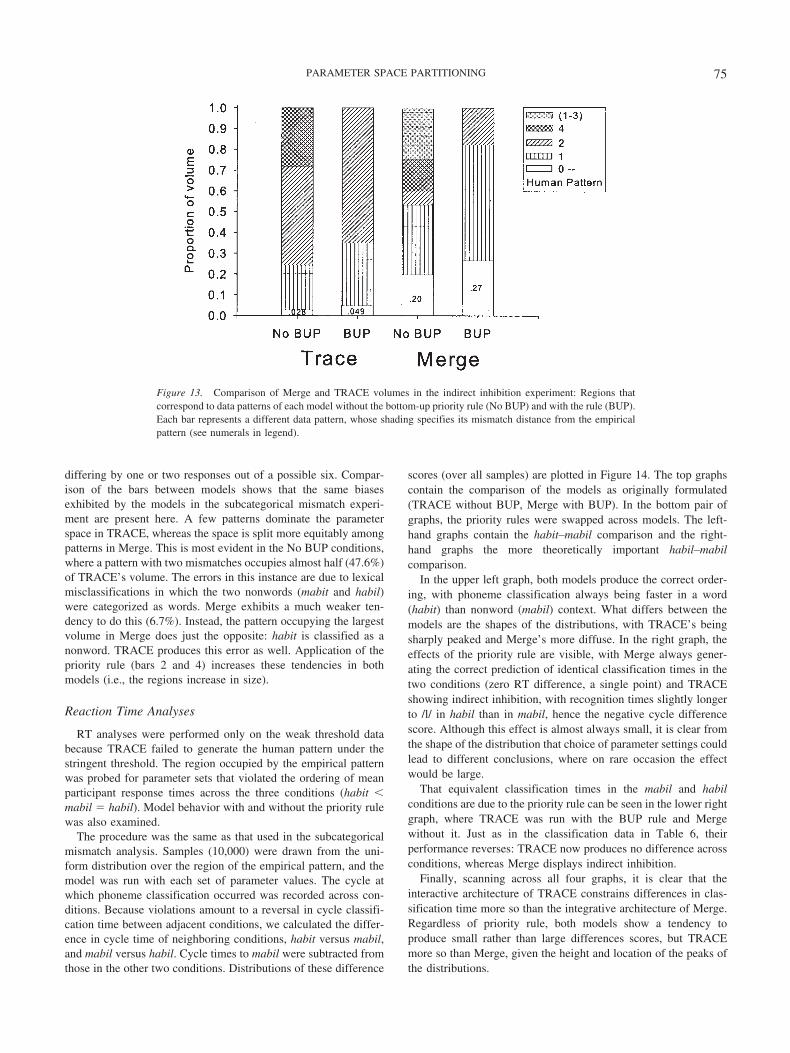
differing by one or two responses out of a possible six. Compar-ison of the bars between models shows that the same biasesexhibited by the models in the subcategorical mismatch experi-ment are present here. A few patterns dominate the parameterspace in TRACE, whereas the space is split more equitably amongpatterns in Merge. This is most evident in the No BUP conditions,where a pattern with two mismatches occupies almost half (47.6%)of TRACE’s volume. The errors in this instance are due to lexicalmisclassifications in which the two nonwords (mabit and habil)were categorized as words. Merge exhibits a much weaker ten-dency to do this (6.7%). Instead, the pattern occupying the largestvolume in Merge does just the opposite: habit is classified as anonword. TRACE produces this error as well. Application of thepriority rule (bars 2 and 4) increases these tendencies in bothmodels (i.e., the regions increase in size).

Reaction Time Analyses

RT analyses were performed only on the weak threshold databecause TRACE failed to generate the human pattern under thestringent threshold. The region occupied by the empirical patternwas probed for parameter sets that violated the ordering of meanparticipant response times across the three conditions (habit �mabil � habil). Model behavior with and without the priority rulewas also examined.

The procedure was the same as that used in the subcategoricalmismatch analysis. Samples (10,000) were drawn from the uni-form distribution over the region of the empirical pattern, and themodel was run with each set of parameter values. The cycle atwhich phoneme classification occurred was recorded across con-ditions. Because violations amount to a reversal in cycle classifi-cation time between adjacent conditions, we calculated the differ-ence in cycle time of neighboring conditions, habit versus mabil,and mabil versus habil. Cycle times to mabil were subtracted fromthose in the other two conditions. Distributions of these difference

scores (over all samples) are plotted in Figure 14. The top graphscontain the comparison of the models as originally formulated(TRACE without BUP, Merge with BUP). In the bottom pair ofgraphs, the priority rules were swapped across models. The left-hand graphs contain the habit–mabil comparison and the right-hand graphs the more theoretically important habil–mabilcomparison.

In the upper left graph, both models produce the correct order-ing, with phoneme classification always being faster in a word(habit) than nonword (mabil) context. What differs between themodels are the shapes of the distributions, with TRACE’s beingsharply peaked and Merge’s more diffuse. In the right graph, theeffects of the priority rule are visible, with Merge always gener-ating the correct prediction of identical classification times in thetwo conditions (zero RT difference, a single point) and TRACEshowing indirect inhibition, with recognition times slightly longerto /l/ in habil than in mabil, hence the negative cycle differencescore. Although this effect is almost always small, it is clear fromthe shape of the distribution that choice of parameter settings couldlead to different conclusions, where on rare occasion the effectwould be large.

That equivalent classification times in the mabil and habilconditions are due to the priority rule can be seen in the lower rightgraph, where TRACE was run with the BUP rule and Mergewithout it. Just as in the classification data in Table 6, theirperformance reverses: TRACE now produces no difference acrossconditions, whereas Merge displays indirect inhibition.

Finally, scanning across all four graphs, it is clear that theinteractive architecture of TRACE constrains differences in clas-sification time more so than the integrative architecture of Merge.Regardless of priority rule, both models show a tendency toproduce small rather than large differences scores, but TRACEmore so than Merge, given the height and location of the peaks ofthe distributions.

Figure 13. Comparison of Merge and TRACE volumes in the indirect inhibition experiment: Regions thatcorrespond to data patterns of each model without the bottom-up priority rule (No BUP) and with the rule (BUP).Each bar represents a different data pattern, whose shading specifies its mismatch distance from the empiricalpattern (see numerals in legend).


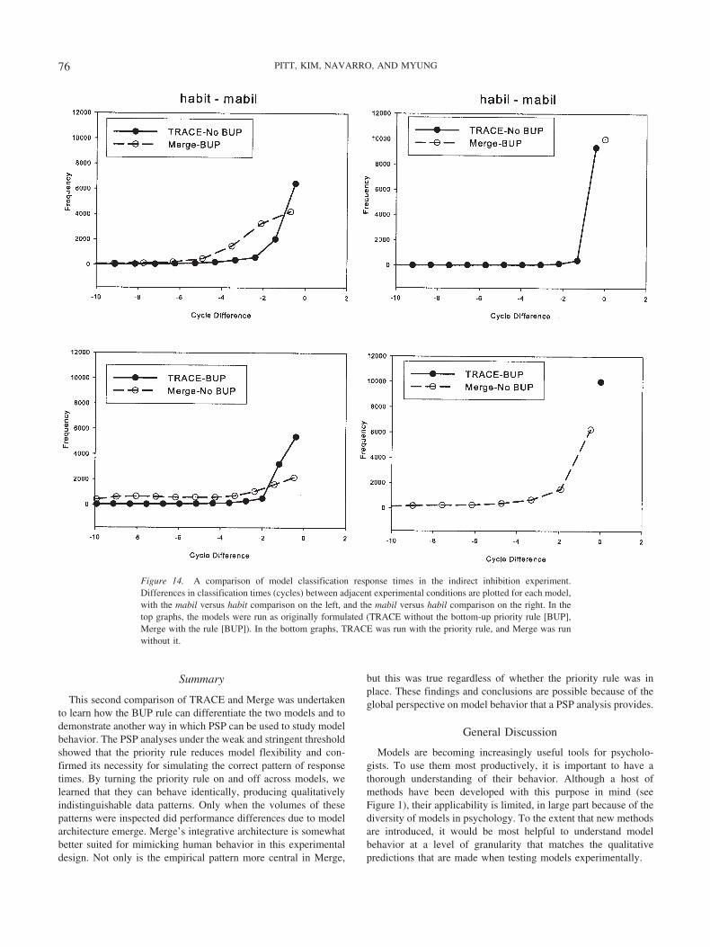
Summary

This second comparison of TRACE and Merge was undertakento learn how the BUP rule can differentiate the two models and todemonstrate another way in which PSP can be used to study modelbehavior. The PSP analyses under the weak and stringent thresholdshowed that the priority rule reduces model flexibility and con-firmed its necessity for simulating the correct pattern of responsetimes. By turning the priority rule on and off across models, welearned that they can behave identically, producing qualitativelyindistinguishable data patterns. Only when the volumes of thesepatterns were inspected did performance differences due to modelarchitecture emerge. Merge’s integrative architecture is somewhatbetter suited for mimicking human behavior in this experimentaldesign. Not only is the empirical pattern more central in Merge,

but this was true regardless of whether the priority rule was inplace. These findings and conclusions are possible because of theglobal perspective on model behavior that a PSP analysis provides.

General Discussion

Models are becoming increasingly useful tools for psycholo-gists. To use them most productively, it is important to have athorough understanding of their behavior. Although a host ofmethods have been developed with this purpose in mind (seeFigure 1), their applicability is limited, in large part because of thediversity of models in psychology. To the extent that new methodsare introduced, it would be most helpful to understand modelbehavior at a level of granularity that matches the qualitativepredictions that are made when testing models experimentally.

Figure 14. A comparison of model classification response times in the indirect inhibition experiment.Differences in classification times (cycles) between adjacent experimental conditions are plotted for each model,with the mabil versus habit comparison on the left, and the mabil versus habil comparison on the right. In thetop graphs, the models were run as originally formulated (TRACE without the bottom-up priority rule [BUP],Merge with the rule [BUP]). In the bottom graphs, TRACE was run with the priority rule, and Merge was runwithout it.


PSP was developed to meet these goals. A model’s ability tomimic human behavior is evaluated in the context of the other datapatterns that it can generate in an experimental design, therebyproviding a richer understanding of what it means for a model toaccount for an experimental result. We specifically chose connec-tionist models to demonstrate PSP’s versatility, as there are fewmethods available for analyzing these widely used yet complexmodels. The method is not limited to this class of models, how-ever. It can be just as easily applied to other types (e.g., algebraic),which makes comparison of models across classes a relativelystraightforward undertaking. PSP’s generality is even evident inthe algorithm’s implementation: A model is a module in thealgorithm, making it possible to insert many types of models.

The three example applications demonstrate only some of whatcan be learned with the method. In the case of ALCOVE, PSP wasused to perform a basic task in model analysis, that is, evaluatingthe model’s soundness in capturing an empirical result. Not onlydid the analysis inform us about whether the model can mimichuman performance (its local behavior), but, much more impor-tantly, by studying the partitioned parameter space, we learnedhow representative this behavior is of the model and how manyother data patterns the model can produce. Some of these wereplausible alternative response patterns. Others occupied such asmall region in the parameter space that they should be consideredspurious and uncharacteristic of the model.

In the second and third applications, PSP was used to study thebehavioral consequences of slight design differences between twolocalist connectionist models. To do this, we compared data pat-terns and their corresponding volumes in parameter space acrossmodels in two experimental settings that were intended to bringout design differences. Many more similarities than differenceswere found in classification behavior. RT analyses of the regionoccupied by the empirical data led to the same conclusion. Qual-itatively, TRACE and Merge were indistinguishable. Only in thevolume analyses did differences emerge. These took the form ofbiases in emphasizing some behaviors over others.

Although one might not be surprised by the models’ similarities,the PSP analysis provides the evidence to solidify such a claim.Furthermore, the analyses suggest how difficult it could be to finda situation in which they make different qualitative predictions thatcould be tested in an experiment. That said, PSP is just the tool toassist in such an endeavor, by enabling the researcher to essentially

pretest an experiment to learn whether it can discriminate betweenmodels. Once an experiment is designed, the models can be runthrough the PSP algorithm to determine which data patterns areshared and which are unique. To the extent that participants arelikely to produce those in the latter category, the experiment hasthe potential to discriminate between the models.

Of course, the meaningfulness of any such analysis depends onhow a data pattern is defined. Conclusions may be specific to adefinition, which is why it is recommended to use more than one.Because ordinal predictions dominate in most experimental work,the task of defining a data pattern can be relatively straightforward.This is another reason why PSP is widely applicable. It does notdepend on quantitative fits.

PSP can also be of considerable use in model development bymaking the modeler aware of the broader consequences of thechoices made in model design. For example, there may be four keyexperimental results that any model of memory must capture to betaken seriously. By running the algorithm in each experimentalsetting, a comprehensive analysis of the model’s design can beundertaken. Desirable and undesirable behaviors can be readilyidentified. The model can then be refined on the basis of thisknowledge and the entire process repeated. From successive iter-ations, one can develop a clear understanding of the model’s innerworkings (e.g., how parameters contribute to model behavior,whether there are redundancies across parameters such as interde-pendency, the appropriateness of their ranges, and even optimalparameter values).

Figure 15 provides a glimpse of what can be learned from suchdetailed analyses. Shown are distributions of parameter values forthree of TRACE’s parameters that were obtained within the em-pirical region of the parameter space in the indirect inhibitionexperiment (no BUP). Each distribution contains 10,000 valuesand gives a sense of how the parameter contributes in capturing theexperimental result. For the phoneme excitation parameter, thedistribution of possible values is fairly broad, although there is aclear optimum. The phoneme-to-word excitation parameter ismuch more tightly constrained, so much so that one might wonderwhether its range should be cut in half, from 0 to 0.5. Thedistribution for the phoneme-to-phoneme inhibition parameter isessentially flat, suggesting a high degree of context sensitivity,which goes along with Norris et al.’s (2000) observations about thestability of indirect inhibition. Analyses such as these expose the

Figure 15. Distributions of values of three TRACE parameters from 10,000 samples of the region in parameterspace corresponding to the empirical data pattern (without the priority rule). Parameter names are listed aboveeach graph.


modeler to tendencies and behaviors that can be difficult to antic-ipate but crucial to know.

Not only can the modeler use this information to enhance themodel itself, but it can also be incorporated into the PSP analysesby, for example, setting prior distributions over parameter rangesto emphasize reasonable behaviors and discount unreasonableones. By default, a PSP analysis assumes the density of pointswithin a region is uniform (i.e., no prior knowledge), but ifmodelers have reason to emphasize certain parameter ranges overothers, then this information can be incorporated into the analysis.This was done in the ALCOVE example, in which parametervalues were restricted to permit only monotonic learning curvesbecause humans do not produce functions of other shapes.

Throughout the article, the global perspective on model behav-ior that PSP provides has been examined from the standpoint of themodel to determine its flexibility or scope (Cutting, 2000). It canbe equally productive to view the situation from the vantage pointof the experiment, by asking how much the experiment is likely tochallenge the model. To the extent that it can, the experiment hasthe potential to be a good, meaningful test of the model. In thisregard, one lesson that comes out of our applications of PSP is thatthe fewer the number of conditions and the fewer the possiblerelationships between them, the less informative the test may be.

The complementary nature of global and local model analysisruns through the preceding discussion. Each informs the other andtogether they improve inference by providing a richer understand-ing of a model’s relationship to data. Qualitative and quantitativemethods are similarly complementary, particularly when examin-ing local model behavior (see Figure 1). Clear model predictionscannot only be tested in an experiment but can further be evaluatedby assessing the model’s fit to data. The use of both can make acompelling case in favor of a model. By going a step further andperforming a global analysis with PSP, additional light can be shedon the quality of the demonstration.

Although fairly general purpose, the current version of PSP isnot applicable to nonstationary models, that is, those whose per-formance can change or adapt as a result of feedback or learning(e.g., some distributed connectionist and algorithmic models). Ofthe large set of models to which PSP is applicable, challenges inimplementation exist on a few fronts. One is in defining a datapattern. In some situations there may be no obvious “natural”definition of a data pattern. A case in point is the power model ofretention (forgetting). The response probability y, representingproportion recall, is a continuous function of retention interval t inthe form of y � at�b where a and b (a, b � 0) are two parameters.Application of PSP requires one to decide whether the retentioncurve associated with parameter values (a, b) � (1.0, 0.5) shouldbe considered indistinguishable, in some defined sense, from thecurve associated with parameter values (a, b) � (1.1, 0.4). In theabsence of a justifiable definition of a data pattern in a situationlike this, it would be preferable to use MDL or Bayesian methodswhen possible. Alternatively, one could devise a “generic,” suit-ably interpretable definition of a data pattern.

Another point to keep in mind when applying PSP is thegenerality of the two types of analyses, counting and volume. Acounting analysis is completely generalizable in the sense that theresults are independent of how the model is parameterized—aproperty known as reparameterization invariance in statistics.What this means is that the data-fitting abilities of the model will

remain unchanged despite different formulations of the model. Toillustrate, consider the functions y � exp [�(a1x1 � a2x2 � a3x3)]and y � b1

x1b2x2b3

x3. These functions are equivalent because the twoare related through the reparameterization bi � exp(�ai), i �1,2,3. Therefore both functions will fit any give data set identi-cally, and consequently, the counting analysis will yield the samenumber of qualitatively different patterns with either parameter-ization. On the other hand, a volume analysis is not reparameter-ization invariant but rather is specific to a particular parameteriza-tion. If each parameter were transformed in an arbitrary way (e.g.,�i�� i � �i

2), one would obtain a different volume analysis unlessthe transformation were positively scaled (i.e., �i�� i, � � 0), inwhich case the results would remain the same.

Depending on the models and testing situation, this lack ofinvariance may be of little practical importance, especially when aspecific parameterization of a model is justified. This is arguablya necessary condition to be considered a model of cognition (Estes,2002). When psychological constructs are associated with partic-ular parameters, constraints can be imposed that prevent arbitrarytransformations. For instance, in the above example, if we assumethat the parameters (a1, a2, a3) represent attention weights, then, bydefinition, they must satisfy the constraints and therefore do notpermit any reparameterization because such a transformationwould alter the interpretations associated with these parameters.

Some models in cognitive science (e.g., FLMP, Oden & Massaro,1978) are nonidentifiable, that is, two or more parameters are per-fectly correlated. What this means is that more than one set ofparameters can yield the same fit to a data set. Parameter redundancylike this is not a problem for PSP, per se, which will successfully mapout the region corresponding to each data pattern. However, as withall models that are nonidentifiable, interpretation of model perfor-mance measures, volume estimates in this case, becomes tricky. Eachpoint in a region could correspond to more than one set of parameters.When it does, which interpretation is correct? Identifying these casescould be challenging as well. Because of these difficulties, beforeapplying PSP, the model should be constrained to make it identifiable(e.g., by fixing the value of one [or more] parameters or equatingparameters), a typical practice in statistics.

Finally, because PSP is a search problem, it is subject to many ofthe same difficulties found in nonlinear function optimization andintegration. Because there are no proven methods for avoiding them,users must find work-arounds to minimize their impact, such asrepeating the simulation with different starting values. PSP is nodifferent in this regard, and this is why we performed multiple runs inthe analyses. Multiple runs provide a measure of the stability, andhence accuracy, of the results. To use PSP productively, the user mustbe aware of the difficulties faced by search methods and have a goodunderstanding of the model being analyzed. Appendix A elaborateson these issues.4

In conclusion, analysis of the global behavior of a model canprovide a wealth of information that is useful for understanding amodel’s performance in a particular testing situation. PSP is a flexibleand powerful method of global model analysis, as the examplespresented here attest, suggesting it has considerable potential to assistresearchers in their quest to model human behavior.

4 Further details on parameter space partitioning are available at http://quantrm2.psy.ohio-state.edu/injae/psp.html.


References

Box, G. E. P. (1976). Science and statistics. Journal of the AmericanStatistical Association, 71, 791–799.

Browne, M. W. (2000). Cross-validation methods. Journal of Mathemati-cal Psychology, 44, 108–132.

Chib, S., & Greenberg, E. (1995). Understanding the Metropolis–Hastingsalgorithm. The American Statistician, 49, 327–335.

Cowles, M. K., & Carlin, B. P. (1996). Markov chain Monte Carloconvergence diagnostics: A comparative review. Journal of the Ameri-can Statistical Association, 91, 883–904.

Cutting, J. (2000). Accuracy, scope, and flexibility of models. Journal ofMathematical Psychology, 44, 3–19.

Dawson, R. W., & Shamanski, K. S. (1994). Connectionism, confusion,and cognitive science. The Journal of Intelligent Systems, 4, 215–262.

Dunn, J. C., & James, R. N. (2003). Signed difference analysis: Theory andapplication. Journal of Mathematical Psychology, 47, 389–416.

Estes, W. K. (2002). Traps in the route to models of memory and decision.Psychonomic Bulletin and Review, 9, 3–25.

Feldman, J. (2000). Minimization of Boolean complexity in human conceptlearning. Nature, 407, 630–633.

Frauenfelder, U. H., Segui, J., & Dijkstra, T. (1990). Lexical effects inphonemic processing: Facilitatory or inhibitory? Journal of Experimen-tal Psychology: Human Perception and Performance, 16, 77–91.

Gelman, A. (1996). Inference and monitoring convergence. In W. R. Gilks,S. Richardson, & D. J. Spiegelhalter (Eds.), Markov chain Monte Carloin practice (pp. 131–140). Boca Raton, FL: Chapman & Hall/CRC.

Gilks, W. R., Richardson, S., & Spiegelhalter, D. J. (1996). Markov chainMonte Carlo in practice. Boca Raton, FL: Chapman & Hall.

Grunwald. P. (1998). The minimum description length principle and rea-soning under uncertainty (ILLG Dissertation Series D5 1998–03). Doc-toral dissertation, Centrum voor Wiskunde en Informatica, Amsterdam,the Netherlands.

Grunwald, P., Myung, I. J., & Pitt, M. A. (2005). Advances in minimumdescription length: Theory and application. Cambridge, MA: MIT Press.

Johansen, M. A., & Palmeri, T. J. (2002). Are there representational shiftsduring category learning? Cognitive Psychology, 45, 482–553.

Kass, R. E., & Raftery, A. E. (1995). Bayes factors. Journal of theAmerican Statistical Association, 90, 773–795.

Kim, W., Navarro, D. J., Pitt, M. A., & Myung, I. J. (2004). An MCMC-based method of comparing connectionist models in cognitive science.Advances in Neural Information Processing Systems, 16, 937–944.

Kontkanen, P., Myllymaki, P., Buntine, W., Rissanen, J., & Tirri, H.(2005). An MDL framework for data clustering. In P. Grunwald, I. J.Myung, & M. A. Pitt (Eds.), Advances in minimum description length:Theory and applications. Cambridge, MA: MIT Press.

Kruschke, J. K. (1992). ALCOVE: An exemplar-based connectionistmodel of category learning. Psychological Review, 99, 22–44.

Kruschke, J. K. (1993). Three principles for models of category learning.The Psychology of Learning and Motivation, 29, 57–90.

Kruschke, J. K., & Erikson, M. A. (1995, November). Six principles formodels of category learning. Paper presented at the 36th annual meetingof the Psychonomic Society, Los Angeles.

Lee, M. D., & Navarro, D. J. (2002). Extending the ALCOVE model ofcategory learning to featural stimulus domains. Psychonomic Bulletinand Review, 9, 43–58.

Luce, R. D. (1963). Detection and recognition. In R. D. Luce, R. R. Bush,& E. Galanter (Eds.), Handbook of mathematical psychology (Vol. 1, pp.103–190). New York: Wiley.

Marslen-Wilson, W., & Warren, P. (1994). Levels of perceptual represen-tation and process in lexical access: Words, phonemes, and features.Psychological Review, 101, 653–675.

McClelland, J. L., & Elman, J. L. (1986). The TRACE model of speechperception. Cognitive Psychology, 18, 1–86.

McCloskey, M. (1991). Networks and theories: The place of connectionismin cognitive science. Psychological Science, 2, 387–395.

McQueen, J., Norris, D., & Cutler, A. (1999). Lexical influence in phoneticdecision making: Evidence from subcategorical mismatches. Journal of Exper-imental Psychology: Human Perception and Performance, 25, 1363–1389.

Myung, I. J. (2000). The importance of complexity in model selection.Journal of Mathematical Psychology, 44, 190–204.

Myung, I. J., Balasubramanian, V., & Pitt, M. A. (2000). Counting prob-ability distributions: Differential geometry and model selection. Pro-ceedings of the National Academy of Sciences, USA, 97, 11170–11175.

Myung, I. J., & Pitt, M. A. (1997). Applying Occam’s razor in modelingcognition: A Bayesian approach. Psychonomic Bulletin and Review, 4,79–95.

Navarro, D. J., & Lee, M. D. (2005, September). An application ofminimum description length clustering to partitioning learning curves.Paper presented at the 2005 IEEE International Symposium on Infor-mation Theory, Adelaide, Australia.

Navarro, D. J., Pitt, M. A., & Myung, I. J. (2004). Assessing the distin-guishability of models and the informativeness of data. Cognitive Psy-chology, 49, 47–84.

Norris, D., McQueen, J. M., & Cutler, A. (2000). Merging information inspeech recognition: Feedback is never necessary. Behavioral and BrainSciences, 23, 299–370.

Nosofsky, R. M. (1986). Attention, similarity and the identification–categorization relationship. Journal of Experimental Psychology: Gen-eral, 115, 39–57.

Nosofsky, R. M., Gluck, M. A., Palmeri, T. J., McKinley, S. C., &Glauthier, P. (1994). Comparing models of rule-based classificationlearning: A replication and extension of Shepard, Hovland, and Jenkins.Memory and Cognition, 22, 352–369.

Oden, G. C., & Massaro, D. W. (1978). Integration of featural informationin speech perception. Psychological Review, 85, 172–191.

Pitt, M. A., Myung, I. J., & Zhang, S. (2002). Toward a method of selectingamong computational models of cognition. Psychological Review, 109,472–491.

Platt, J. R. (1964). Strong Inference, Science, 146, 347–353.Rissanen, J. (1996). Fisher information and stochastic complexity. IEEE

Transactions on Information Theory, 42, 40–47.Rissanen, J. (2001). Strong optimality of the normalized ML models as

universal codes and information in data. IEEE Transactions on Infor-mation Theory, 47, 1712–1717.

Robert, C. P., & Casella, G. (1999). Monte Carlo statistical methods. NewYork: Springer.

Roberts, S., & Pashler, H. (2000). How persuasive is a good fit? Acomment on theory testing. Psychological Review, 107, 358–367.

Shepard, R. N. (1987). Toward a universal law of generalization forpsychological science. Science, 237, 1317–1323.

Shepard, R. N., Hovland, C. L., & Jenkins, H. M. (1961). Learning andmemorization of classification. Psychological Monographs 75(13,Whole No. 517).

Shiffrin, R., & Nobel, P. (1998). The art of model development and testing.Behavior Research Methods, Instruments and Computers, 29, 6–14.

Shiffrin, R., & Steyvers, M. (1997). A model for recognition memory:REM—Retrieving effectively from memory. Psychonomic Bulletin andReview, 4, 145–166.

Stone, M. (1974). Cross-validatory choice and assessment of statisticalpredictions [with discussion]. Journal of Royal Statistical Society, SeriesB, 36, 111–147.

Wagenmakers, E.-J., Ratcliff, R., Gomez, P., & Iverson, G. J. (2004).Assessing model mimicry using the parametric bootstrap. Journal ofMathematical Psychology, 48, 28–50.

(Appendixes follow)


Appendix A

The PSP Algorithm in Greater Detail

PSP is a search problem that attempts to answer the question, How doesone determine the range of data patterns a model can generate? Theproblem is addressed by first adopting a particular definition of a datapattern. In doing so, one induces an unknown but finite partition on theparameter space of a model, with each region corresponding to a datapattern. The goal is to design a search procedure that visits each of theseunknown regions at least once. Model analyses follow from what is learnedfrom the search.

Difficulties Inherent in a Sampling-Based Approach

An intuitive approach for finding regions is to sample the parameterspace enough times to ensure that each region is sampled at least once. Inthis approach, one is effectively randomly sampling parameter values fromsome distribution and then checking to see whether these produce a newregion. In a naive, simple Monte Carlo (SMC) approach, this would be auniform distribution over the whole parameter space. As the number ofsamples drawn increases, this procedure will uncover all regions of non-zero volume with probability 1. However, as the dimensionality of themodel increases, SMC becomes inefficient quite rapidly. An unreasonablylarge number of samples is required for accurate estimation. This problemis commonly referred to as the curse of dimensionality, and it forces us toturn to more efficient search methods. In essence, this amounts to findinga better probability distribution from which to sample.

One of the major inefficiencies in SMC search is that it takes no accountof the fact that some regions are much larger than others. With the goal ofPSP being to visit each search region at least once, it is inefficient to spendmost of one’s time in a few big regions, which is what would happen witha uniform distribution. Thus, an ideal sampling distribution would be onethat assigns equal probability to every region in the partition. In short, anatural way to improve on SMC would be to rescale the parameter spaceso that all regions are treated as being the same size. Our PSP algorithmuses a Markov chain Monte Carlo (MCMC) procedure to perform this kindof rescaling.

PSP Sampling by MCMC: The Basic Idea

MCMC (Gilks et al, 1996) is a powerful method for sampling a com-plicated target distribution, denoted f(�). The assumption is that we knowhow to calculate the value of f(�), but have no simple method of samplingfrom it. The Metropolis–Hastings algorithm (see Chib & Greenberg, 1995)provides such a method. One begins by specifying a jumping distribution(described more fully below), denoted q(�k|�k�1), which is used to samplecandidate points by “jumping” around in the target distribution. Withprobability a � min{[f(�k)q(�k�1|�k)] / [f(�k�1)q(�k|�k�1)], 1}, the nextsampled point is �k. However, with probability 1 � a, we stay in the samespot (i.e., the next point is �k�1). The ergodicity of the algorithm guaran-tees that the frequency distribution of the sampled points converges to thetarget distribution.

Recall that our goal was to specify a target distribution that is uniformover the regions in parameter space. Obviously it is impossible to specifythis distribution directly, given that the partition itself is unknown. How-ever, we can specify a series of approximations to this ideal distributionthat will eventually converge to it, under certain assumptions. At any givenpoint in the search, the PSP algorithm will have discovered some numberof regions. To ensure that each of the discovered regions is treated equally,we run a separate Markov chain, using the Metropolis–Hastings algorithmfor each of these regions, each with a different target distribution that isuniform on that region (i.e., f(�) � c0 for some positive constant c0 if �belongs to the region, and f(�) � 0 otherwise). A uniform target distribu-

tion is used because we want to generate a series of accepted points that areevenly sampled over the region. On any given sampling trial, we randomlypick one of these chains from which to draw the next sample (or system-atically sweep through all of them in order to be more efficient), therebyensuring that samples are drawn from each of the discovered regionsequally often irrespective of size. After enough trials, this mixture ofsamples will approximate the target distribution over the regions.

“Growing” the Partition: How PSP Finds Regions

The procedure outlined above has the rather awkward property ofconverging to the ideal target distribution (uniform on each region) so longas the algorithm has already discovered all the regions, which rather defeatsthe point of the search. In order to address this problem, we need to ensurethat the algorithm looks outside of the discovered regions often enough toensure that it finds new regions. Our approach to discovering new regionsis based on the assumptions that new regions will be found along the edgesof old regions (“contiguity”; see below). It also helps if adjacent regions arecorrelated in size. A natural way to find regions that satisfy this assumptionis to adapt the jumping distribution to ensure that the Markov chains jumpoutside of these regions at an ideal rate. To understand why this approachsucceeds, recall that the target distribution for a given MCMC routine isuniform on a particular region so that points that lie outside the region willalways be rejected. If the parameter space meets the aforementionedconditions, all regions will be found.

Another aspect of our approach is that whenever a new region isencountered, the PSP algorithm concentrates solely on that region until ithas “caught up” to the pre-existing regions in terms of the number ofsamples drawn from it. (If multiple new regions are found, they are queueduntil they all catch up.) The reason for this is that the discovery of a newregion is essentially a source of information about a potentially informativearea of the parameter space that has not yet been fully explored. Accord-ingly, as we wish to treat all regions equally, the algorithm concentrates ona new region until it is on an equal footing with all the regions that werepreviously discovered. By deliberately ensuring that the various chainsfrequently jump outside their borders, the PSP algorithm is constantly“looking” for new regions. In sum, the algorithm aggressively searches fornew regions in the vicinity of a newly discovered region at a level ofgranularity that is scaled to the size of the current region.

The Jumping Distribution

As the previous discussion should make clear, the choice of a jumpingdistribution is critical to the success of the PSP algorithm, even though itis chosen independently of the target distribution and serves only as thesource from which to generate candidate points. We have used a uniformdistribution over a hypersphere centered on the current location in theparameter space. The reason for using a hypersphere is that it is widelyused in cases where the sampling region is constrained and no priorinformation is available about the shape of the region; the hypersphericalshape of a jumping distribution is least likely to favor a particular shape ofthe sampling domain a priori.

In PSP, the size of the jumping distribution (i.e., the radius of thehypersphere) must adapt to each region. If it is too small, almost allcandidate points will be accepted, but every jump will be so small that itwill take too many jumps for an exhaustive search of a new region. Also,rejected points, by which new regions outside the current region are beingdiscovered, will rarely be generated. In contrast, if the size of the jumpingdistribution is too large, candidate points will be rejected too often, and thegranularity of the jumps will not be small enough to define the edges of a


region, which requires a properly sized jumping distribution to succeed.Unfortunately, unless one is dealing with a normal distribution, no theoryexists that defines the optimal jumping distribution.

With the PSP algorithm, we have found it best to adapt the size of thejumping distribution so that the Markov chain on average accepts 20% to25% of the candidate points. In other words, each chain spends 20–25% ofits time moving around inside the region and the rest of its time searchingfor new regions just outside the borders. This range was identified heuris-tically by testing the algorithm on real and toy models many times withjumping distributions that varied widely in size. Two performance mea-sures were used in these tests: search speed and the variance of the region’svolume estimates. The goal was to find an acceptance rate for the jumpingdistribution that maximized search speed and minimized the variance ofvolume estimates.

Formal Description of the PSP Algorithm

Having presented the main concepts underlying PSP, we are now in aposition to define the search algorithm formally.

Initialize. Given �1 and Pattern 1, set m � i � 1.

Step 1. Establish qm (�|�) by adapting the size of its hypersphericaldomain. Go to Step 2.

Step 2. Set i � mod(i, m) � 1. Go to Step 3.

Step 3. Sample �y from qi (�|�i). If �y generates a new valid pattern, setm � m � 1, set �m � �y, record the new pattern as pattern m, and thengo to Step 1. If �y generates pattern i, set �i � �y and go to Step 2.Otherwise, go to Step 2.

In the algorithm, qi (�|�i) denotes the jumping distribution of the regioncorresponding to pattern i, centered at �i. The subscript 1 � i � m indexesthe region from which we are currently sampling, and m represents thenumber of regions found thus far. The algorithm terminates when a presetnumber of search trials (i.e., size of an MCMC chain) is obtained for eachof the discovered regions. Several analytic methods are available to helpdetermine how many search trials must be used for the series to convergeto the target distribution and to determine the number of initial draws,called “burn-ins,” to discard from the analysis (Cowles & Carlin, 1996;Gelman, 1996).

Note that the initial conditions (Step 0) require an initial parameter set(i.e., point in parameter space) in order to start the algorithm. These can beprovided in one of two ways. First, we could run a preliminary SMC searchto find a parameter set that yields a valid pattern. Alternatively, if themodeler has good intuitions about which parameter sets generate valid datapatterns, these can be used as the initial starting values.

Assumptions When Using PSP

For the PSP algorithm to succeed in finding all data patterns, someassumptions must be met. They are the following:1. Continuity. A data pattern occupies a single continuous region in theparameter space, such that any two points that produce the pattern can bejoined by a path that passes only through points that produce that samepattern.2. Contiguity. Regions are contiguous with one another in the sense thatany two regions can be joined by a path that passes only through points thatproduce a valid data pattern.3. Stationarity. Model behavior is stationary in the sense that a givenparameter set always generates a single, fixed data pattern. This means thatthe boundaries of the regions are fixed, not varying every time the modelgenerates a data pattern.

Among these three conditions, the first two (continuity and contiguity)are key conditions necessary for the algorithm to perform satisfactorily.

That is, the assumption that the region is continuous is implicit in Step 1and the contiguity condition is necessary for Step 3. In the followingpassage, we discuss how potential violations of all three can be detectedand handled if suspected.

The assumptions of continuity and contiguity are reasonable if thecomputational model being analyzed is composed of mathematical func-tions that are known to exhibit these properties (i.e., the functions arecontinuous and smooth). If these assumptions are suspected of beingviolated (e.g., there are breaks in the range of a parameter), the modeler cancheck the consistency of the PSP solution through multiple runs of thealgorithm. Estimated center or mean points and covariance matrices ofdiscovered regions, which are output by the algorithm, will reveal incon-sistencies, such as discrepant volume estimates or the number of datapatterns found. Inspection of these values across multiple PSP runs shouldvalidate any suspicions and reveal the nature of the inconsistency, if itexists.

For example, if one suspects the existence of noncontiguous regions inthe parameter space, creating “islands” of data patterns, then there are atleast two remedies one can use to ensure PSP finds them. One is to run thePSP algorithm supplied with different initial starting points. The modeler,who is most familiar with the behavior of the model, should be able toprovide parameter values that generate typical patterns as well as lesstypical patterns that could come from another region in the parameterspace. The more parameter values the modeler can provide, the more likelythe algorithm will find the noncontiguous regions, if they are present.Another method for finding noncontiguous regions is to use SMC. That is,one would randomly sample the parameter space to find such islands.Large regions are of most importance because the data from them couldinfluence PSP performance. Fortunately, size works to the modeler’sadvantage in this circumstance because a reasonably long run of SMCshould be able to find at least one point in an island. Once this is done, thePSP algorithm can take over from there and find the other elements of thepartition that belong to the island.

To test this idea, we ran a simulation test in which islands of datapatterns were placed in various regions of the parameter space. The resultsshowed that SMC worked quite well and found all islands in a reasonableamount of time for models of up to seven dimensions. At higher dimen-sions, the islands become such tiny specks in the model’s parameter spacethat exponentially longer runs are needed to find them, which can quicklybecome impractical, leading to a drop in the success rate. Work is currentlyunder way to devise a more efficient method for finding islands in higherdimensions.

These same two approaches to discovering noncontiguous regions canbe used to identify discontinuous regions that correspond to the same datapattern. Multiple runs with different initial points or a preliminary SMC runcan help detect such discontinuous regions, again especially if they occupyconsiderable individual volumes. Output analyses conducted with esti-mated center points, volumes, and the covariance matrix of discoveredregions will reveal their existence and location through discrepanciesacross repeated measurements.

The stationarity assumption implies that PSP is not applicable tosimulation-based, probabilistic models (e.g., distributed connectionistmodels, algorithmic models such as REM; Shiffrin & Steyvers, 1997).For this reason, a probabilistic model can be analyzed by PSP only if itssimulational component can be replaced with a closed-form probabilitydensity (or mass) function, so that data patterns are defined on the spaceof probability distributions. Implementation of an algorithm such asPSP requires dealing with other issues as well. Many of these arepractical in nature but have the potential to influence the results. Forexample, if neighboring regions are similar in size, there is a goodchance of finding them because the probability of sampling from asimilarly-sized region is higher than that of a much smaller region. Ifone suspects that tiny regions are nestled between larger ones, then thebest course of action is to increase the sample size so that the likelihood


(Appendixes continue)

of landing in these tiny regions isgreater. The use of multiple runs, asdiscussed above, will also help in this regard. Other pragmatic issuesinclude ensuring that the parameter ranges are finite and definingappropriate stopping criteria.A1 The preceding discussion is intended toalert potential users of PSP to the issues that must be considered whenapplying it. Our sampling-based approach to partitioning the parameterspace makes it a powerful tool for model analysis, but like othernumerical methods that work in high dimensions, including MCMC andnonlinear optimization, correct answers are not guaranteed and cannotbe proved in general settings, except for trivial cases. This is why

heuristics must be devised and used during application of the method tocombat potential problems. Their purpose is to minimize anomalousresults and ensure that an answer is accurate and trustworthy.

A1 To assist the user in addressing these and related issues when usingPSP, the Web site (see Footnote 4) provides the Matlab source code of thecurrent algorithm and future updates, along with a tutorial that covers thesetopics in detail.

Appendix B

A Test of the Accuracy of Volume Estimation

The ability to analyze the volumes of regions is an attractive feature ofPSP. Nevertheless, it must be recognized that it is nontrivial to estimate thevolume of an arbitrary multidimensional object with no closed-form shapeand location. Volume estimation was performed in two steps, both involv-ing sampling-based methods. In the first, a region’s border is approximatedwith an ellipsoid defined by the estimated mean vector and covariancematrix of the MCMC sample of the region. If we use the volume of thisellipsoid as a first approximation to the volume of the region, the resultshould be biased toward overestimation because an ellipsoid is an “evenlypacked” object in every possible direction, and data patterns are not likelyto have similarly simple, compact shapes. Because of this, the amount ofbias should be related to the degree to which the region is concave (all orpart of it). This bias can affect the volume analysis because the degree ofconcavity may differ across regions being compared.

The second step of volume estimation adjusts for this bias with thehit-or-miss method of Monte Carlo integration. First, a random sample ofsize n is drawn from the uniform distribution over the ellipsoid. Next, theratio of the number of sample points within the region (i.e., the “hits”) tothe total number of samples, n, is used as a factor of bias correction. Thisvalue is then multiplied by the volume of the ellipsoid to obtain the finalvolume estimate of the region. Our expectation in using this two-stepprocedure was that any bias of underestimation after adjustment would benegligible compared with the overestimation before adjustment. Nonethe-less, it was necessary to assess the severity of the bias in order to determinehow it might limit analyses using the volume measure.

We therefore designed a very stringent simulation test to assess theaccuracy of volume estimation. A region in a multidimensional space wasrandomly generated in the following way. On an evenly spaced grid in thisspace, a cell was selected as a starting point of the region. The region wasthen expanded (i.e., grew) into one of its orthogonally neighboring cells ina random direction, to form a two-celled region. The region was expandedagain into a neighboring cell, adjacent to any part of the region, not just thenew cell. This process was repeated until this randomly shaped region, R,filled a preset number or cells. Its volume, VR, was estimated by PSP withthe equation,

VR�k

nVd�d � 2d/ 2|S|1/ 2

where Vd is the volume of a d-dimensional sphere of radius 1, S is thecovariance matrix estimated from the MCMC output, and k is the numberof sample points in region R out of all n points in the ellipsoid.

Accuracy was measured by comparing the estimated volumes of two ofthese arbitrarily shaped regions. The ratio of these two volumes was usedas the measure of accuracy, for which the known, true ratio served as thereference point. It is important to understand that it is not appropriate tocompare the estimated volume of a region with its “true” volume. The

reason is that the scale of the parameter space is arbitrary, so the value ofa region’s volume is not meaningful by itself. The value is meaningful onlyin comparison with another region’s volume, which is how the measurewas used in our three application examples and how it was used in this test.

The simulation was carried out using a two-factorial design that yieldeda variety of situations in which PSP’s volume estimation method might beused in real applications. The number of dimensions of the parameter spacewas the first variable. There were three levels (4, 7, 10), which were chosen

Figure B1. Volume ratio estimates for a given dimensionality, d, acrossthe six cell–number pairs. Values greater than one indicate a bias inoverestimating volume.


to cover a range of models in use in the discipline. The second factor wasthe number of cells used to form each of the two randomly shaped regions(3, 10, 30, 100). All four levels were completely crossed (e.g., 3 and 10, 3and 30, 3 and 100) to increase the diversity of possible shapes beingcompared, which was meant to further increase the realism and difficultyof the test. Note that because of the algorithm’s scale-adapting ability, asdiscussed in Appendix A, it does not pose an obstacle for comparingregions whose volumes constitute a different number of cells (e.g., 3 vs.30). The two regions were simply scaled to have the same volume so thattheir ratio should be one in all comparisons.

Because the region-generation method described above was highly un-constrained (requiring only continuity between cells), the 10-, 30-, and100-cell regions had the potential to have extremely bizarre shapes (e.g.,multipronged objects in various directions and dimensions). As a result,conditions 3 and 30, 3 and 100, and 10 and 100 were likely to be the mostchallenging pairings. The accuracy of volume estimation was pushed to thelimits in these cases.

In each of the pairings across dimensionality, the region-generation andvolume-estimation and -comparison process was repeated 300,000 times.Regions were sampled 60,000 times (for ellipsoid estimation) and 15,000times (for the hit-or-miss adjustment) on each trial, which is equivalent tothe five multiple runs used in the Merge and TRACE analyses. A subset ofthe results, which includes the most difficult cases, is shown in Figure B1.Each panel shows the distribution of volume ratio estimates for a givendimensionality d across the different cell–number pairs. The ratio of the

larger estimate to the smaller was used, so values greater than one indicatethe size of error in volume comparison.

Across most pairing trials, volume estimation was good, with the peaksof the distributions at or near 1.0 and the tails falling off sharply so that fewvalues exceeded 1.5, even when d � 10. Errors were greatest for thepairings in which cell numbers differed most (3 and 100, 10 and 100), andthis tendency was magnified with dimensionality. Nevertheless, the bias issurprisingly modest, as the 3 and 100 comparison is a full order ofmagnitude larger than the 3 and 10 pairing, yet the means for the twodistributions differ by only 0.163 (1.234 and 1.071, respectively). Whenthis same test was performed without the hit-or-miss volume-adjustmentstep, biases were much more severe, with the peaks of error distributionsfar beyond 1.0, especially when the number of dimensions and cells waslarge.

In sum, the results of this test demonstrate that although volume esti-mation can be biased, its robustness across a wide range of region shapesindicates that the method is reasonably accurate and trustworthy most ofthe time. For the models used in the present study, volume differencesbetween regions were exponentially large. To view them all on the samegraph, we had to plot them on a log scale (e.g., Figure 8). Thus, it goeswithout saying that the volume estimation method is more than sufficientlyaccurate to use rank-ordered estimates in analyzing the volumes of param-eter regions, regardless of their shape. In most instances, comparison on aninterval scale is appropriate.

Appendix C

TRACE and Merge Parameters

Parameter TRACE Merge Range

Phoneme excitation � � (0,1)Phoneme to word excitation � � (0,1)Phoneme to word inhibition � (0,1)Phoneme to target excitation � (0,1)Phoneme decay � � (0,1)Word to target excitation � (0,1)Word to phoneme excitation � (0,1)Word to word inhibition � � (0,1)Word decay � � (0,1)Target to target inhibition � (0,1)Target decay � (0,1)Target momentum � (0,1)Phoneme to phoneme inhibition � (0,1)Cycles per input slice � � Fixed

Note. The word to word inhibition parameter was used in the indirect inhibition example.

Received August 24, 2004Revision received June 28, 2005

Accepted June 29, 2005 �


Documents

Global Model Analysis by Parameter Space Partitioning