Embed Size (px)
Citation preview

Air Force Institute of TechnologyAFIT Scholar
Theses and Dissertations Student Graduate Works
3-14-2014
Optimal Partitioning of a Surveillance Space forPersistent Coverage Using Multiple AutonomousUnmanned Aerial Vehicles: An IntegerProgramming ApproachUmar M. Khan
Follow this and additional works at: https://scholar.afit.edu/etd
This Thesis is brought to you for free and open access by the Student Graduate Works at AFIT Scholar. It has been accepted for inclusion in Theses andDissertations by an authorized administrator of AFIT Scholar. For more information, please contact [email protected].
Recommended CitationKhan, Umar M., "Optimal Partitioning of a Surveillance Space for Persistent Coverage Using Multiple Autonomous Unmanned AerialVehicles: An Integer Programming Approach" (2014). Theses and Dissertations. 681.https://scholar.afit.edu/etd/681

OPTIMAL PARTITIONING OF A SURVEILLANCESPACE FOR PERSISTENT COVERAGE USING
MULTIPLE AUTONOMOUS UNMANNED AERIALVEHICLES: AN INTEGER PROGRAMMING
APPROACH
THESIS
Umar M. Khan, Major, USAF
AFIT-ENS-14-M-16
DEPARTMENT OF THE AIR FORCEAIR UNIVERSITY
AIR FORCE INSTITUTE OF TECHNOLOGYWright-Patterson Air Force Base, Ohio
DISTRIBUTION STATEMENT A. APPROVED FOR PUBLIC RELEASE;
DISTRIBUTION IS UNLIMITED

The views expressed in this thesis are those of the author and do not reflect the officialpolicy or position of the United States Air Force, the United States Department of Defenseor the United States Government. This is an academic work and should not be used toimply or infer actual mission capability or limitations.

AFIT-ENS-14-M-16
OPTIMAL PARTITIONING OF A SURVEILLANCE SPACE
FOR PERSISTENT COVERAGE USING MULTIPLE
AUTONOMOUS UNMANNED AERIAL VEHICLES:
AN INTEGER PROGRAMMING APPROACH
THESIS
Presented to the Faculty
Department of Operational Sciences
Graduate School of Engineering and Management
Air Force Institute of Technology
Air University
Air Education and Training Command
in Partial Fulfillment of the Requirements for the
Degree of Master of Science (Operations Research)
Umar M. Khan, BS, MS Ed
Major, USAF
March 2014
DISTRIBUTION STATEMENT A. APPROVED FOR PUBLIC RELEASE;
DISTRIBUTION IS UNLIMITED

AFIT-ENS-14-M-16
OPTIMAL PARTITIONING OF A SURVEILLANCE SPACE
FOR PERSISTENT COVERAGE USING MULTIPLE
AUTONOMOUS UNMANNED AERIAL VEHICLES:
AN INTEGER PROGRAMMING APPROACH
Umar M. Khan, BS, MS EdMajor, USAF
Approved:
//signed// 24 March 2014
James W. Chrissis, PhD (Chair) Date
//signed// 24 March 2014
Darryl K. Ahner, PhD (Member) Date
//signed// 24 March 2014
LTC Brian J. Lunday, PhD (Member) Date

AFIT-ENS-14-M-16
Abstract
Unmanned aerial vehicles (UAVs) are an essential tool for the battlefield commander in
part because they represent an attractive intelligence gathering platform that can quickly
identify targets and track movements of individuals within areas of interest. In order to
provide meaningful intelligence in near-real time during a mission, it makes sense to op-
erate multiple UAVs with some measure of autonomy to survey the entire area persistently
over the mission timeline. This research considers a space where intelligence has identi-
fied a number of locations and their surroundings that need to be monitored for a period of
time. An integer program is formulated and solved to partition this surveillance space into
the minimum number of subregions such that these locations fall outside of each partitioned
subregion for efficient, persistent surveillance of the locations and their surroundings. Par-
titioning is followed by a UAV-to-partitioned subspace matching algorithm so that each
subregion of the partitioned surveillance space is assigned exactly one UAV. Because the
size of the partition is minimized, the number of UAVs used is also minimized.
iv

To my wife and my baby boy...
v

Acknowledgements
I would like to acknowledge Dr. James Chrissis, my advisor and thesis committee chair
for all of the help and advice. In addition, Lieutenant Colonel Brian Lunday (US Army),
Ph.D., and Dr. Darryl Ahner also deserve credit for great inputs and guidance along the
way as committee members. Finally, my colleagues - fellow officers in the operations
research program (both master’s and Ph.D. students) - helped me get through some of the
course work and provided an ear when I needed one. To all of those mentioned above, I say
“thank you,” and I hope I am afforded an opportunity to work with you again in the future.
Umar M. Khan
vi
Table of Contents
Page
Abstract . . . . . . . . . . . . . . . . . . . . . . . . . . . . . . . . . . . . . . . . . . . . . . . . . . . . . . . . . . . . . . . . . . iv
Acknowledgements . . . . . . . . . . . . . . . . . . . . . . . . . . . . . . . . . . . . . . . . . . . . . . . . . . . . . . . . . vi
List of Figures . . . . . . . . . . . . . . . . . . . . . . . . . . . . . . . . . . . . . . . . . . . . . . . . . . . . . . . . . . . . . ix
List of Tables . . . . . . . . . . . . . . . . . . . . . . . . . . . . . . . . . . . . . . . . . . . . . . . . . . . . . . . . . . . . . . xi
I. Introduction . . . . . . . . . . . . . . . . . . . . . . . . . . . . . . . . . . . . . . . . . . . . . . . . . . . . . . . . . . . 1
1.1 Background . . . . . . . . . . . . . . . . . . . . . . . . . . . . . . . . . . . . . . . . . . . . . . . . . . . . . . . 11.1.1 Persistent Surveillance . . . . . . . . . . . . . . . . . . . . . . . . . . . . . . . . . . . . . . . . 3
1.2 Problem Statement . . . . . . . . . . . . . . . . . . . . . . . . . . . . . . . . . . . . . . . . . . . . . . . . . 51.3 Research Objective and Scope . . . . . . . . . . . . . . . . . . . . . . . . . . . . . . . . . . . . . . . 51.4 Assumptions . . . . . . . . . . . . . . . . . . . . . . . . . . . . . . . . . . . . . . . . . . . . . . . . . . . . . . 61.5 Summary . . . . . . . . . . . . . . . . . . . . . . . . . . . . . . . . . . . . . . . . . . . . . . . . . . . . . . . . . 6
II. Literature Review . . . . . . . . . . . . . . . . . . . . . . . . . . . . . . . . . . . . . . . . . . . . . . . . . . . . . . 8
2.1 Introduction . . . . . . . . . . . . . . . . . . . . . . . . . . . . . . . . . . . . . . . . . . . . . . . . . . . . . . . 82.2 Previous Work . . . . . . . . . . . . . . . . . . . . . . . . . . . . . . . . . . . . . . . . . . . . . . . . . . . . . 8
2.2.1 Path Planning . . . . . . . . . . . . . . . . . . . . . . . . . . . . . . . . . . . . . . . . . . . . . . . 82.2.2 Area Decomposition . . . . . . . . . . . . . . . . . . . . . . . . . . . . . . . . . . . . . . . . 27
2.3 Summary . . . . . . . . . . . . . . . . . . . . . . . . . . . . . . . . . . . . . . . . . . . . . . . . . . . . . . . . 48
III. Methodology . . . . . . . . . . . . . . . . . . . . . . . . . . . . . . . . . . . . . . . . . . . . . . . . . . . . . . . . . 49
3.1 Introduction . . . . . . . . . . . . . . . . . . . . . . . . . . . . . . . . . . . . . . . . . . . . . . . . . . . . . . 493.2 Surveillance Space Partitioning . . . . . . . . . . . . . . . . . . . . . . . . . . . . . . . . . . . . . . 49
3.2.1 Integer Programming Partitioning Formulation . . . . . . . . . . . . . . . . . . 543.3 UAV Assignment . . . . . . . . . . . . . . . . . . . . . . . . . . . . . . . . . . . . . . . . . . . . . . . . . 583.4 Partitioning and Assignment Flowchart . . . . . . . . . . . . . . . . . . . . . . . . . . . . . . . 643.5 Operational Scenarios . . . . . . . . . . . . . . . . . . . . . . . . . . . . . . . . . . . . . . . . . . . . . 653.6 Summary . . . . . . . . . . . . . . . . . . . . . . . . . . . . . . . . . . . . . . . . . . . . . . . . . . . . . . . . 65
IV. Implementation and Analysis . . . . . . . . . . . . . . . . . . . . . . . . . . . . . . . . . . . . . . . . . . . 68
4.1 Introduction . . . . . . . . . . . . . . . . . . . . . . . . . . . . . . . . . . . . . . . . . . . . . . . . . . . . . . 684.2 Implementation . . . . . . . . . . . . . . . . . . . . . . . . . . . . . . . . . . . . . . . . . . . . . . . . . . . 684.3 Analysis . . . . . . . . . . . . . . . . . . . . . . . . . . . . . . . . . . . . . . . . . . . . . . . . . . . . . . . . . 70
4.3.1 Partitioning and Assignment . . . . . . . . . . . . . . . . . . . . . . . . . . . . . . . . . . 704.3.2 Special Cases . . . . . . . . . . . . . . . . . . . . . . . . . . . . . . . . . . . . . . . . . . . . . . 744.3.3 Postprocessing . . . . . . . . . . . . . . . . . . . . . . . . . . . . . . . . . . . . . . . . . . . . . 75
vii

Page
4.3.4 Logistics . . . . . . . . . . . . . . . . . . . . . . . . . . . . . . . . . . . . . . . . . . . . . . . . . . 774.4 Summary . . . . . . . . . . . . . . . . . . . . . . . . . . . . . . . . . . . . . . . . . . . . . . . . . . . . . . . . 78
V. Conclusions and Recommendations . . . . . . . . . . . . . . . . . . . . . . . . . . . . . . . . . . . . . . 80
5.1 Introduction . . . . . . . . . . . . . . . . . . . . . . . . . . . . . . . . . . . . . . . . . . . . . . . . . . . . . . 805.2 Review . . . . . . . . . . . . . . . . . . . . . . . . . . . . . . . . . . . . . . . . . . . . . . . . . . . . . . . . . . 805.3 Insights . . . . . . . . . . . . . . . . . . . . . . . . . . . . . . . . . . . . . . . . . . . . . . . . . . . . . . . . . 825.4 Potential Future Research . . . . . . . . . . . . . . . . . . . . . . . . . . . . . . . . . . . . . . . . . . 82
5.4.1 Expand Pool of UAVs . . . . . . . . . . . . . . . . . . . . . . . . . . . . . . . . . . . . . . . 835.4.2 Probabilistic Models . . . . . . . . . . . . . . . . . . . . . . . . . . . . . . . . . . . . . . . . 835.4.3 Model Camera Footprint . . . . . . . . . . . . . . . . . . . . . . . . . . . . . . . . . . . . . 83
5.5 Conclusion . . . . . . . . . . . . . . . . . . . . . . . . . . . . . . . . . . . . . . . . . . . . . . . . . . . . . . . 83
A. Excel R© VBA Code . . . . . . . . . . . . . . . . . . . . . . . . . . . . . . . . . . . . . . . . . . . . . . . . . . . . 86
B. MATLAB R© Code . . . . . . . . . . . . . . . . . . . . . . . . . . . . . . . . . . . . . . . . . . . . . . . . . . . . . 92
Bibliography . . . . . . . . . . . . . . . . . . . . . . . . . . . . . . . . . . . . . . . . . . . . . . . . . . . . . . . . . . . . . 106
viii
List of Figures
Figure Page
1. Cyclic Schedule ([27], p. 13) . . . . . . . . . . . . . . . . . . . . . . . . . . . . . . . . . . . . . . . . 12
2. T IC3 problem with two UAVs, ([14], p. 5) . . . . . . . . . . . . . . . . . . . . . . . . . . . . . 19
3. Front camera FOV ([15], p. 1) . . . . . . . . . . . . . . . . . . . . . . . . . . . . . . . . . . . . . . . 22
4. Left camera FOV ([15], p. 2) . . . . . . . . . . . . . . . . . . . . . . . . . . . . . . . . . . . . . . . . 22
5. Two samples of tesselated coverage area ([15], p. 6) . . . . . . . . . . . . . . . . . . . . 24
6. Path and final entropy ([36], p. 6) . . . . . . . . . . . . . . . . . . . . . . . . . . . . . . . . . . . . 26
7. Example minimum Manhattan network ([20], p. 3) . . . . . . . . . . . . . . . . . . . . . 27
8. Equitable Partitioning: TSP Tours . . . . . . . . . . . . . . . . . . . . . . . . . . . . . . . . . . . . 29
9. Equitable Partitioning: Population . . . . . . . . . . . . . . . . . . . . . . . . . . . . . . . . . . . 30
10. Polygon with vertices . . . . . . . . . . . . . . . . . . . . . . . . . . . . . . . . . . . . . . . . . . . . . . 31
11. Image pyramid over terrain . . . . . . . . . . . . . . . . . . . . . . . . . . . . . . . . . . . . . . . . . 32
12. Area partition ([31], p. 8) . . . . . . . . . . . . . . . . . . . . . . . . . . . . . . . . . . . . . . . . . . . 33
13. lawnmower pattern search ([31], p. 8) . . . . . . . . . . . . . . . . . . . . . . . . . . . . . . . . 33
14. Hexagonal and quadrangular grid decompositions . . . . . . . . . . . . . . . . . . . . . . 33
15. Two-cell persistent coverage . . . . . . . . . . . . . . . . . . . . . . . . . . . . . . . . . . . . . . . . 35
16. Age of cells, left first ([34], p. 3) . . . . . . . . . . . . . . . . . . . . . . . . . . . . . . . . . . . . . 36
17. Age of cells, right first ([34], p. 3) . . . . . . . . . . . . . . . . . . . . . . . . . . . . . . . . . . . . 36
18. Recursive partition of a rectangular space ([34], p. 7) . . . . . . . . . . . . . . . . . . . . 37
19. Possible optimal paths from A to B ([34], p. 11) . . . . . . . . . . . . . . . . . . . . . . . . 38
20. RGP examples with cuts . . . . . . . . . . . . . . . . . . . . . . . . . . . . . . . . . . . . . . . . . . . . 40
21. Elements of RGP . . . . . . . . . . . . . . . . . . . . . . . . . . . . . . . . . . . . . . . . . . . . . . . . . . 41
22. Infeasible RGP partitioning elements . . . . . . . . . . . . . . . . . . . . . . . . . . . . . . . . . 41
ix

Figure Page
23. Canonical rectangle examples . . . . . . . . . . . . . . . . . . . . . . . . . . . . . . . . . . . . . . . 45
24. Feasible rectangles composed of canonicals . . . . . . . . . . . . . . . . . . . . . . . . . . . 46
25. Point configuration of a Class III constraint ([32], p. 17) . . . . . . . . . . . . . . . . . 46
26. Point configurations . . . . . . . . . . . . . . . . . . . . . . . . . . . . . . . . . . . . . . . . . . . . . . . 47
27. Notional minimal partition . . . . . . . . . . . . . . . . . . . . . . . . . . . . . . . . . . . . . . . . . . 51
28. Corectilinearity . . . . . . . . . . . . . . . . . . . . . . . . . . . . . . . . . . . . . . . . . . . . . . . . . . . 52
29. Minimum length, minimum partition I . . . . . . . . . . . . . . . . . . . . . . . . . . . . . . . . 54
30. Minimum length, minimum partition II . . . . . . . . . . . . . . . . . . . . . . . . . . . . . . . 55
31. Example operational scenarios . . . . . . . . . . . . . . . . . . . . . . . . . . . . . . . . . . . . . . . 56
32. Example induced grids . . . . . . . . . . . . . . . . . . . . . . . . . . . . . . . . . . . . . . . . . . . . . 57
33. Example scenarios solved . . . . . . . . . . . . . . . . . . . . . . . . . . . . . . . . . . . . . . . . . . . 58
34. UAV categories ([5], p. 9) . . . . . . . . . . . . . . . . . . . . . . . . . . . . . . . . . . . . . . . . . . 60
35. UAV assignment process . . . . . . . . . . . . . . . . . . . . . . . . . . . . . . . . . . . . . . . . . . . 62
36. Camera swath width and rectangle width . . . . . . . . . . . . . . . . . . . . . . . . . . . . . . 63
37. High-level depiction of partitioning and assignment process . . . . . . . . . . . . . . 64
38. Scenarios: Set I . . . . . . . . . . . . . . . . . . . . . . . . . . . . . . . . . . . . . . . . . . . . . . . . . . . 66
39. Scenarios: Set II . . . . . . . . . . . . . . . . . . . . . . . . . . . . . . . . . . . . . . . . . . . . . . . . . . 67
40. Solutions to scenarios in Set I . . . . . . . . . . . . . . . . . . . . . . . . . . . . . . . . . . . . . . . 69
41. Solutions to scenarios in Set II . . . . . . . . . . . . . . . . . . . . . . . . . . . . . . . . . . . . . . . 70
42. All points diagonally collinear . . . . . . . . . . . . . . . . . . . . . . . . . . . . . . . . . . . . . . . 75
43. Loading RQ-8B Fire Scout onto C-17 Globemaster III . . . . . . . . . . . . . . . . . . 77
44. Global Hawk Emerging from C-5 Galaxy ([4]) . . . . . . . . . . . . . . . . . . . . . . . . . 78
x
List of Tables
Table Page
1. Variable definitions for T IC3 planner . . . . . . . . . . . . . . . . . . . . . . . . . . . . . . . . . 18
2. Average maximum age, comparing EDP and ADP . . . . . . . . . . . . . . . . . . . . . . 39
3. UAV characteristics: Global Hawk, Shadow, and Raven . . . . . . . . . . . . . . . . . 61
xi

OPTIMAL PARTITIONING OF A SURVEILLANCE SPACE
FOR PERSISTENT COVERAGE USING MULTIPLE
AUTONOMOUS UNMANNED AERIAL VEHICLES:
AN INTEGER PROGRAMMING APPROACH
I. Introduction
Unarmed, unmanned aerial vehicles will be the tool of choice to monitorthe activities of armed groups and the movement of civilians.
– BBC News Africa, quoting Herve Ladsous, UN Peacekeeping chief in theDemocratic Republic of the Congo [10]
1.1 Background
An unmanned aerial vehicle (UAV) carries a suite of sensors and sometimes armament,
and it is usually controlled by personnel situated at a geographically separated location or
perhaps near the range where the UAV is operating. While these vehicles have at times been
referred to as Remotely Piloted Aircraft (RPA), Unmanned Aerial Systems (UAS), and
more colloquially as “drones”, they are referred to as UAVs in this research. Fixed-wing
and rotary-wing UAVs are in production today, and several organizations make use of them.
For example, the 2012 USAF Almanac lists three fixed-wing UAVs operated by the United
States Air Force today in theater operations - The MQ-1 Predator, MQ-9 Reaper, and RQ-4
Global Hawk [6]. As another example, the United States Navy operates the rotary-wing
RQ-8 Fire Scout to “provide reconnaissance, situational awareness, and precision targeting
support for ground, air and sea forces” [12]. Government organizations not part of the
Department of Defense (DoD), such as the Department of Homeland Security (DHS) and
1
law enforcement agencies, also use these aerial vehicles. In fact, the DHS not only makes
use of UAVs, but is accelerating the integration of UAVs into law enforcement agencies for
potential use over US airspace [40]. Finally, even some commercial entities are researching
novel ways to conduct business using unmanned aircraft. In 2013, Jeff Bezos, CEO of
online retailer Amazon, declared that within four to five years, his company would be able,
on a limited basis, to deliver packages quickly to customers using a UAV delivery system
[17].
Because of the many potential applications of UAVs, the industry that develops and
markets these vehicles has responded by designing a wide variety of UAVs in terms of
capability, size, takeoff and landing method, fuel, allowable payloads, and other factors.
These various UAVs come in many forms. For example, considering exclusively the mili-
tary applications of UAVs, the ScanEagle surveillance platform weighs 37.9 pounds, has a
wingspan of just 10.2 feet and is fueled by gasoline. The much larger RQ-4A Global Hawk
has a gross weight of 26,750 pounds, carries no weapons, has a wingspan of 116.2 feet, and
runs on JP-8 fuel. Finally, the rotary-wing MQ-8B Fire Scout weighs about 2,070 pounds
empty and can be modified to carry weapons. [3] The plethora of available UAVs is just
one indication of their prominence in both domestic and international affairs dealing with
security and commerce. Further importance of UAV surveillance capabilities is clear, given
the DoD’s position that the reconnaissance and surveillance mission remains the number
one combatant command priority for unmanned systems [3].
The importance of UAVs to military intelligence gathering means that there may need
to be many UAVs in the collective inventories of the U.S. armed forces. Because resources
are limited, the DoD cannot simply acquire an unlimited number of UAVs to perform mis-
sions. That truth is underscored by the fact that the United States is now in an era of
government sequestration in which the fastest growing occupation in the United States Air
Force - war zone surveillance - is generating budget decisions that call for the produc-
2
tion of billions of dollars worth of UAVs [23]. However, not everyone is convinced that
this rate of expenditure on UAVs is warranted. In an article for National Defense, former
Secretary of the Air Force Michael Donley suggested that the parallel growth of manpower
requirements warrants a re-look at UAV procurement activities. He expressed that spending
on intelligence-surveillance-reconnaissance (ISR) capabilities might be excessive because
such investments may be duplicating funding efforts by other military departments. In the
same article, former Vice Chief of Staff of the Army General Peter Chiarelli stated, “With
leaner times approaching and U.S. forces in Afghanistan drawing down, the Pentagon may
no longer afford or need so much ISR support.” Chiarelli noted that the military depart-
ments may have too much overlap in UAV capabilities and that these could be cut down,
considering the redundancies now in place, in order to reduce unnecessary spending. [23]
This research considers exclusively a nonlethal military application of multiple UAVs.
Specifically, the concern is with the problem of persistent surveillance, which is the use of
a team of UAVs to cover an area of land while meeting time over target constraints. The
term “persistent surveillance” is a source of confusion, but it is defined precisely in Section
1.1.1 in contrast to several other terms that are often taken as synonymous in the literature.
Some key assumptions and restrictions will also apply and are described later, in Section
1.4.
1.1.1 Persistent Surveillance.
To understand precisely what “persistent surveillance” means, it is defined explicitly
here because it is not a term that is used in the same sense across the literature. For ex-
ample, Joint Publication 2-0 [9] uses the term, but fails to define it. Joint Publication 2-01
[7] defines persistent coverage as “near-continuous surveillance capability of the area of
interest as opposed to periodic reconnaissance.” Although that language is closer to how
it is used here, it is still not precise enough to formulate the problem at hand. The DoD
3

Dictionary [8] defines persistent surveillance as “A collection strategy that emphasizes the
ability of some collection systems to linger on demand in an area....” This definition is not
sufficient for this research because it is too vague to provide a good foundation for a precise
formulation. Finally, a report produced by the Army Science Board in 2008 [2] based on
a study involving surveillance states, “Persistence is not well defined.” The definition of
persistent used in the Army study was: “If I have what I need, when I need it, for as long
as I need it, it is persistent.” Because of the confusion surrounding the term “persistent
surveillance,” the definitions that follow differentiate between that term and other terms
that are sometimes taken as synonymous.
Definition I.1. Persistent surveillance is surveillance of an area of land by a collection
of vehicles over a mission timeline such that none of a specified collection of pre-defined
points of interest on the ground is left unobserved for longer than a defined, usually small
(relative to mission timeline), amount of time.
Definition I.2. Continuous surveillance is surveillance of an area of land by a collection
of vehicles over a mission timeline such that none of a specified collection of pre-defined
points of interest on the ground is left unobserved at any time. Further, when the points
of interest encompass every point on the area of land to be observed, then the program of
surveillance is termed total continuous surveillance.
Definition I.3. Standby surveillance refers to the availability of a surveillance platform
within the vicinity of points of interest over a surveillance space. The vicinity of those
points is defined by a commander or other decision maker in the area of operations.
Definition I.4. Periodic surveillance is surveillance of an area of land based on a schedule.
In this case, vehicles observe a location for a period of time, depart, return after a period of
time, and continue this pattern on a regular schedule as determined by a decision maker.
This research uses the term “persistent surveillance” as it is defined in Definition I.1, which
is essentially the definition used by Nigam and Kroo [34]. In practice, this persistent
4

surveillance is best executed by autonomous UAVs. The UAVs are considered autonomous
in the sense that no significant human interaction is required from the time the vehicles are
launched on a mission to the time they prepare to return to the base of operations. That is,
the UAVs are preprogrammed to fly a particular pattern over their assigned regions.
1.2 Problem Statement
Given an area of land R and set P of interior locations of interest, the problem is to
generate a persistent UAV surveillance program, using the minimum number of UAVs, that
sweeps all of R continually over a mission timeline while revisiting locations in P within
a specified time increment. To be clear, this is a two-fold problem. The first part of the
problem is to decide how to minimize the number of UAVs that move over the space to
provide persistent surveillance. The second part involves deciding which particular UAVs
should be used to carry out the surveillance program such that the revisit time constraint is
met for each of the points in P.
1.3 Research Objective and Scope
The objective of this research is to describe a way to determine an optimal assignment
of UAVs to an area of land for automatic surveillance for a specified period of time. Here,
optimal means utilizing the minimum number of UAVs to persistently cover a given surveil-
lance space with minimum revisit times over specified locations within the space. Covered
in this research are methods for partitioning areas into smaller mutually exclusive, collec-
tively exhaustive areas and ways to assign UAVs to partitioned subregions of a surveillance
space. Also covered is a brief discussion on the logistics of delivering UAVs to areas of
operation as well as future work.
5

1.4 Assumptions
A few important assumptions apply to this research, and they are listed in this section.
1. The UAVs fly in uncontested airspace. This is possible if air supremacy is first
achieved, which is also assumed.
2. Launch, recovery, and maintenance operations occur near enough to the area of land
that is of interest to effectively carry out the program of surveillance.
3. Not all available UAVs have the same characteristics. Some UAVs are small and
more capable of covering smaller areas through line of sight control while others can
stay aloft on the order of days and sweep large areas.
4. All available UAVs are capable of being pre-programmed to fly with a measure of
autonomy over the surveillance space. This is not a critical assumption, but rather it
is a suggestion of how to implement the surveillance program effectively.
5. A UAV is considered to have covered a point over the surveillance space if it flies
over that point. In other words, for simplicity, the precise physical characteristics of
the UAV payload, i.e., its sensors, are not taken into account. The cameras might
be pointed to the side or in a forward direction, but the problem is simplified here
by modeling the camera swath as transverse to the fuselage, extending horizontally
along the craft’s roll axis.
6. The UAVs fly at slightly different altitudes in order to avoid colliding with one an-
other.
1.5 Summary
Using UAVs to observe a section of land has some clear advantages over relying on
ground intelligence, solely on satellite imagery, or on manned aircraft alone. Ground in-
6

telligence carries the most risk to both U.S. military forces and local residents of the area
of operations, and is therefore not desirable if less risky alternatives can provide equivalent
intelligence (in cases where what we are interested in is images and movement of people
in the area of interest). Satellites cannot be dedicated to a specific spot on the earth without
extensive pre-planning, constellation design, and orbital analysis. This requires massive
amounts of resources in terms of time and money, and such an undertaking is not normally
used to survey ad hoc areas of interest, but rather long-term, strategic interests (for exam-
ple, the nuclear launch sites of a foreign power). In contrast, UAVs are designed for just
such missions where we need to collect information on the fluid movements of potential
targets and on locations where suspicious activity may be taking place.
Pilots flying traditional aircraft can persistently survey an area just as autonomous
UAVs can, but using manned aircraft to conduct persistent surveillance makes less sense
than using UAVs to do the same. Persistent surveillance is a task best left to a mechanical
device, not a human being who is naturally prone to error and even more likely to commit
errors performing such a repetitive area sweep over long periods of time. Thus, for good
reason, it makes sense to use UAVs that can operate in an autonomous fashion to conduct
persistent surveillance in an area of operations.
7
II. Literature Review
2.1 Introduction
Covering or providing surveillance over an area of land using one or more UAVs has
been studied from many different angles. There are as many variations on the problem as
there are methods for formulating and solving them. This chapter presents some of those
many varieties of the coverage problem and discusses how researchers have approached the
task of formulating and solving associated models.
2.2 Previous Work
2.2.1 Path Planning.
Several researchers have addressed the problem of covering an area using UAVs. There
are many different ways to define the problem and also many ways to solve the problems so
defined. The specific case addressed in this research concerns persistent surveillance, and
certainly, this is a topic that has been studied. To better understand the persistent coverage
problem, we consider the many ways UAV coverage in general has been defined before
considering persistent coverage specifically, because the methods of defining and solving
all such problems are instructive.
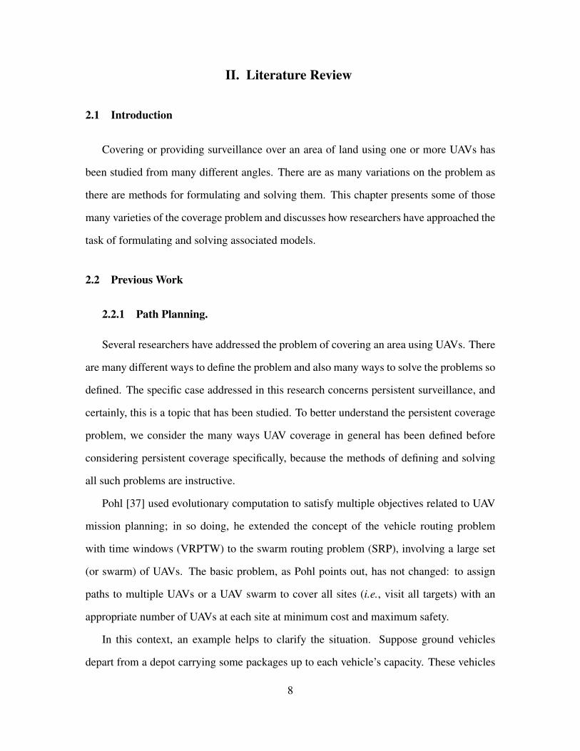
Pohl [37] used evolutionary computation to satisfy multiple objectives related to UAV
mission planning; in so doing, he extended the concept of the vehicle routing problem
with time windows (VRPTW) to the swarm routing problem (SRP), involving a large set
(or swarm) of UAVs. The basic problem, as Pohl points out, has not changed: to assign
paths to multiple UAVs or a UAV swarm to cover all sites (i.e., visit all targets) with an
appropriate number of UAVs at each site at minimum cost and maximum safety.
In this context, an example helps to clarify the situation. Suppose ground vehicles
depart from a depot carrying some packages up to each vehicle’s capacity. These vehicles
8
must deliver their packages to a set of locations within some time window for each delivery.
Further, each location is to be visited only once by a vehicle. The depot itself is also open
during a specific time window only - it can be considered as just another site to visit. The
task is to determine the shortest set of paths such that all packages are delivered within
their time windows and all vehicles return to the depot before it closes. This model can
be applied to UAVs delivering a camera package over sites defined to be ground space
that needs to be observed by at least one UAV within specified time windows (say, within
every five minutes). In that case, persistent coverage of the battlespace can be modeled as
a VRPTW.
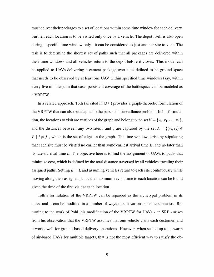
In a related approach, Toth (as cited in [37]) provides a graph-theoretic formulation of
the VRPTW that can also be adapted to the persistent surveillance problem. In his formula-
tion, the locations to visit are vertices of the graph and belong to the set V = v0,v1, · · · ,vn,
and the distances between any two sites i and j are captured by the set A = (vi,v j) ∈
V | i 6= j, which is the set of edges in the graph. The time windows arise by stipulating
that each site must be visited no earlier than some earliest arrival time E, and no later than
its latest arrival time L. The objective here is to find the assignment of UAVs to paths that
minimize cost, which is defined by the total distance traversed by all vehicles traveling their
assigned paths. Setting E = L and assuming vehicles return to each site continuously while
moving along their assigned paths, the maximum revisit time to each location can be found
given the time of the first visit at each location.
Toth’s formulation of the VRPTW can be regarded as the archetypal problem in its
class, and it can be modified in a number of ways to suit various specific scenarios. Re-
turning to the work of Pohl, his modification of the VRPTW for UAVs - an SRP - arises
from his observation that the VRPTW assumes that one vehicle visits each customer, and
it works well for ground-based delivery operations. However, when scaled up to a swarm
of air-based UAVs for multiple targets, that is not the most efficient way to satisfy the ob-
9

jectives. Instead, Pohl argues that using a swarm of UAVs exploits the divisibility of the
swarm and route subgroups of UAVs to different targets in parallel, having them regroup at
other targets. This avoids the inefficiency of sending one vehicle to one target at a time.
The SRP formulation begins the same way as the VRPTW. In the SRP, there is a de-
pot and a number of vehicles that must depart from the depot, service a number of cus-
tomers within specified time windows, and return to the depot before it closes. Much of the
VRPTW formulation carries over to the SRP; in particular, the same overall graph structure
with the same nomenclature for the vertices and edges holds as in the VRPTW. Each cus-
tomer in this case is a target having its own time window beginning at the earliest arrival
time E, and ending at its latest arrival time L. Time L is the time by which a UAV must
arrive at the target in order to complete service and still be able to return to the depot be-
fore it closes. Arriving early results in waiting time W . Where the SRP diverges from the
VRPTW is that demand in the SRP is indicated by the number of UAVs that need to be at a
target within its time window for the duration of the service time. Before, in the VRPTW,
demand was satisfied by vehicle capacity. Also, in the VRPTW, service time is the time
needed to make a delivery (e.g., get an answer at the door, transfer the package, receive a
signature, exchange pleasantries, etc.), but in the SRP service time is defined by the time
UAVs need to spend over a target. To simplify problem complexity, Pohl stipulates that
UAVs only split into or join sub-swarms at targets.
With these considerations in place, the objective of the SRP is to determine the set
of paths for the UAVs such that the total distance is minimized, and the formulation is
identical to that of the VRPTW, with a few exceptions. In the VRPTW, each vehicle has
some capacity defined by what it can carry, but in the SRP, the capacity is defined by a
UAV’s travel capacity. In addition, the VRPTW calls for each location to be visited by only
one vehicle. This constraint is removed in the SRP formulation. Demand at locations in
10

the SRP is also defined differently from demand in the VRPTW. In the SRP, the demand at
a location is defined by the number of UAVs that must visit the location.
Suppose there are more objectives for the mission than just meeting demand at a set
of targets, and there is a need to continuously revisit targets over a period of time. Maybe
using a minimum number of UAVs to perform the mission is important. In those cases,
one objective function is inefficient, and a multiobjective optimization problem may be in-
dicated. Pohl’s [37] model represents just such a multiobjective optimization problem. In
fact, Pohl considers what happens if a vehicle exceeds its capacity to service a route, arrives
early, or arrives late. In these cases, a swarm of UAVs can split into multiple subswarms,
adding UAVs to the groups when necessary, to travel to multiple targets in parallel. Pohl’s
multiobjective formulation of the SRP then requires an adjustment to the objective func-
tion, namely, adding more functions to optimize. The main modification here is based on
the fact that wait time is defined by the difference between a UAV’s arrival time and the
arrival time of the latest UAV, if the latest arrival time is past the earliest service time at a
location. The reason for this is that all vehicles that are required to be on target to service it
must be in place before service can begin. Pohl points out that a multiobjective formulation
to this UAV routing problem is more effective because the problem has an irregular solu-
tion space, stating, “Time constraints introduce irregularities to the Pareto front such that
non-dominated solutions become more isolated.” Pohl’s approach is to use evolutionary
algorithms to solve his multiobjective problem.
Ha [27] looks at the task of continuously covering an area of land using the minimum
number of UAVs. Sometimes, Ha argues, continuous coverage can net important results
that would otherwise be out of reach. For example, during Operation Iraqi Freedom, it
was 600 hours of continuous surveillance of an Al-Qaeda leader that led to his demise;
moreover, a gap in the coverage could have given the targeted individual an opening to
escape. Based on these considerations, Ha develops a cyclic scheduling approach to deter-
11

mine the minimum number of UAVs to cover an area of land continuously. To understand
his approach, consider K UAVs comprising the set F = (∆1,T1),(∆2,T2), · · · ,(∆K,TK).
If Vi = (∆i,Ti), then, F = V1,V2, · · · ,VK, where Vi is the attribute vector of UAV i. The
variable ∆i is the UAV’s round trip time and Ti its loiter time. Further the variable ∆i itself
is an aggregation of three components for UAV i: ξi1, the time from base of operations
to target; ξi2, the time from target back to the base of operations; and ξ
i3, time spent in
maintenance and repairs at the operating base. Thus, ∆i = ξi1 + ξ
i2 + ξ
i3.
Having expressed the attribute vectors of the UAVs, Ha then sets about defining a cyclic
schedule in this context. First, the expression Vi→ Vj denotes that UAV i does a mission
handoff to UAV j. If that mission handoff is successful, then, he writes Vis−→Vj. An ordered
sequence of UAVs E = (Vi1,Vi2 , · · · ,ViK ), where Vi j = (∆i j ,Ti j), j = 1,2, · · · ,K is called a
cyclic schedule if Vi1 → Vi2 → ··· → ViK−1 → ViK → Vi1 . This situation is illustrated in
Figure 1, which depicts a cyclic schedule of size 6, corresponding to having six UAVs.
Figure 1. Cyclic Schedule ([27], p. 13)
Each directed arc in the figure depicts a mission handoff from the originating node to
the terminal node. So, at a given target, UAV 2 arrives to receive a handoff from UAV 1
just as UAV 1 is ready to depart for base. When UAV 2 arrives, it loiters for time T2 and
hands off to UAV 3, and the process continues. A cycle is said to be completed when UAV
12

6 hands off to UAV 1. Any particular UAV is only used once in each cycle and when not
in use, it is in “rest” at the base for refueling and maintenance. Critically, as Ha shows,
continuous coverage is assured with N ≥ 2 UAVs such that (N − 2)T < ∆ ≤ (N − 1)T .
Then, a schedule with N UAVs allows continuous coverage and one with N− 1 or fewer
UAVs introduces coverage gaps at a particular target. The problem then becomes one of
minimizing N such that the schedule has no coverage gaps.
What Ha found was that continuous coverage is only possible in the deterministic case
and that the number of UAVs required is increasing in round-trip time and decreasing in
loiter time (assuming the other is held constant). Ha first considers this deterministic case
with a homogeneous fleet of UAVs and then with a nonhomogeneous fleet, formulating both
as scheduling problems. It is in this context that he introduces the concept of a minimum
cyclic schedule that he uses to compute a schedule using the minimum number of UAVs
to continuously cover a target area. In that case, the ratio T/∆ becomes a performance
measure for a UAV; a large value for the ratio indicates that a UAV loiters longer with less
support from other UAVs. Finally, he considers the stochastic case (both risk-neutral and
risk-averse) in which UAVs have attributes that follow some probability distribution. The
stochastic formulation introduces coverage gaps [27].
Ha provides s a linear programming formulation to find an optimal cyclic schedule that
allows continuous coverage of the target area. The linear programming formulation begins
with the definition of a binary decision variable, x j as
x j =
1, if UAV j is included in the schedule
0, otherwise.
Thus, the objective is: minz =K
∑i=1
xi. The feasible region of the linear program is the set
of all feasible cyclic schedules. For convenience, Ha relabels Ti as ai and ∆i as bi, where i
13
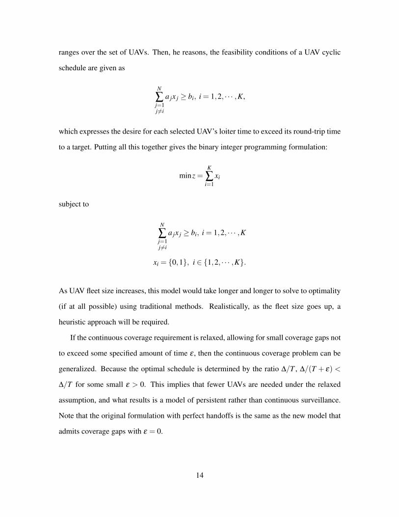
ranges over the set of UAVs. Then, he reasons, the feasibility conditions of a UAV cyclic
schedule are given as
N
∑j=1j 6=i
a jx j ≥ bi, i = 1,2, · · · ,K,
which expresses the desire for each selected UAV’s loiter time to exceed its round-trip time
to a target. Putting all this together gives the binary integer programming formulation:
minz =K
∑i=1
xi
subject to
N
∑j=1j 6=i
a jx j ≥ bi, i = 1,2, · · · ,K
xi = 0,1, i ∈ 1,2, · · · ,K.
As UAV fleet size increases, this model would take longer and longer to solve to optimality
(if at all possible) using traditional methods. Realistically, as the fleet size goes up, a
heuristic approach will be required.
If the continuous coverage requirement is relaxed, allowing for small coverage gaps not
to exceed some specified amount of time ε , then the continuous coverage problem can be
generalized. Because the optimal schedule is determined by the ratio ∆/T , ∆/(T + ε) <
∆/T for some small ε > 0. This implies that fewer UAVs are needed under the relaxed
assumption, and what results is a model of persistent rather than continuous surveillance.
Note that the original formulation with perfect handoffs is the same as the new model that
admits coverage gaps with ε = 0.
14
If the target area is dynamic and if contact with the ground station and between UAVs
is desired, then a trade space arises between achieving good coverage and maintaining con-
nectivity. This problem of coverage in wireless sensor networks is important and has been
investigated by many. Along these lines, Yanmaz [41] considers using autonomous UAVs
to survey an area of land with such constraints. The UAVs must maintain connectivity with
a ground station and with each other at all times. He presents a probabilistic connectivity-
based mobility model for a network of autonomous UAVs. In [41], UAV autonomy means
that each UAV decides its own path taking into account only its communication require-
ment. The trade space arises because of UAV transmission ranges. A given area can be
sensed faster if UAV coverage overlap is minimized, but the UAVs may need to fly closer
to each other in order to stay connected and to be able to deliver the sensed data to the
ground station.
Traditionally, mobility models for sensor networks have been coverage-based; an ex-
ample is found in Yanmaz and Guclu (as cited in [41]). In the example, there is an assumed
repulsive force between UAVs; at any given navigation decision point, a UAV, say UAV 1
in a network of (suppose) four UAVs, would experience a collection of repulsive forces that
act on it by the other UAVs. The resultant force vector ~R1 is the vector sum of the forces
incident on UAV 1, and the net force on UAV 1 is given by ~R1 = ∑j
~Fj1. This forces UAV
1 to travel in the direction of vector ~R1. Further, the forces acting on UAV 1 are inversely
proportional to the distances from UAV 1 to the other UAVs - the closer UAVs come to each
other, the harder they push on each other. In addition, UAV 1 experiences a force inversely
proportional to its sensing range in the direction of its motion, which ensures that the UAV
avoids retracing already covered areas.
Whereas in the coverage-based model each UAV computes a resultant force and moves
accordingly, in a connectivity-based model, UAVs take communication into account. The
algorithm Yanmaz proposes has the UAVs using only their current location and direction to
15
maintain contact with each other and the ground station. The algorithm is general enough
to allow for a heterogeneous network of UAVs that can enter and leave the system as they
surveil an area of land that may not be fixed. Because the algorithm is probabilistic, mo-
mentary loss of contact between a UAV and the ground station can occur, but it is highly
unlikely that a UAV will become isolated, and if so, highly unlikely it would be isolated for
very long.
Yanmaz compares the coverage-based and connectivity-based UAV motion models
when the ground station is in the corner of the surveillance space and also when it is in the
center. What he finds is that a critical spatial density is required for the connectivity-based
model to be an efficient coverage plan. Further, the location of the ground station affects
the connectivity-based mobility model by a scaling factor only. As for transmission range,
as that increases, spatial coverage gets better in the connectivity-based model because as
sensing range increases, the UAVs can spread out more and the system tends desirably
toward less sensing overlap. Yanmaz also investigates how the system behaves under a
single-hop assumption versus a multi-hop assumption. In a single-hop scenario, coverage-
based mobility performs better as the number of UAVs increases, but performance is not
significantly improved in the connectivity-based model as the number of UAVs increases.
Moving to the multi-hop scheme, however, the performance gap shrinks; then, the im-
portant factor in coverage and communication becomes spatial density, or, the number of
UAVs over the surveillance space [41].
Ahmadzadeh, Buchman, Cheng, Jadbabaie, Keller, Kumar, and Pappas [14] use a dif-
ferent approach to the UAV coverage problem. They consider planning the trajectories
of multiple autonomous UAVs to maximize spatio-temporal coverage such that the UAVs
avoid collisions and satisfy initial and final position requirements. They developed al-
gorithms with the needs of two programs in mind: DARPA HURT (Defense Advanced
Research Projects Agency Heterogeneous Urban RSTA (reconnaissance, surveillance and
16
target acquisition) Team) and the Office of Naval Research (ONR) Intelligent Autonomy
program. The Intelligent Autonomy program focuses on developing software to coordinate
autonomous UAVs, USVs (unmanned surface vehicles), and UUVs (unmanned undersea
vehicles).
In [14], Ahmadzadeh, et al. design the Time Critical Coverage (T IC3) planning tool
as part of the Integrated Cognitive-Neuroscience Architectures for Understanding Sense-
making (ICARUS) project, which is one of several projects under the Intelligent Autonomy
program of the ONR. The T IC3 planning tool starts when it receives a request for a motion
plan for each of several vehicles under its control, along with the entry and exit state for
each vehicle - information such as three-dimensional location, velocity vector, and arrival
time. The planning tool then requests information on obstacles, threat zones, and sensor
availability, which then allows it to determine the largest area that can be covered. It out-
puts not way-points but secondary objective points complementing the primary mission set
in paths between entry and exit. If needed, the planning tool can be invoked more than once
during a mission as required. The authors note that the problem has been addressed using
cellular decomposition, where a cell is considered covered when traversed by a UAV (or
when it scans the entire cell, usually using a boustrophedon or lawnmower, back-and-forth
motion), but they also note that this has been used mainly in the single-robot situation. Also,
most prior work in area coverage has focused on sensor networks. Instead, Ahmadzadeh,
et al. use a sampling-based technique to cover an area.
Because T IC3 is a variation of the motion planning problem (with optimality consider-
ations), it is normally an NP-hard problem. However, the T IC3 problem is constrained by
a time budget. As such, they needed an efficient way to get good solutions. To that end,
they formulate a sampling-based technique for area coverage. The variables used in the
formulation are given in Table 1.
17

Table 1. Variable definitions for T IC3 planner
Variable Definition
N Number of heterogeneous autonomous vehiclesvi Constant forward velocity of vehicle iwi ∈Wi Controllable turning rate of vehicle ixi = (px
i , pyi ,θi) ∈ Xi State of vehicle i: position (px
i , pyi ), orientation θi
pentry(exit)i , tentry(exit)
i Boundary position and time conditionsΩ⊂ R2 Coverage area, union of polygonal regionsO⊂ R2 No-travel zones, union of polygonal regionsΨ Sensor footprint mapping; Ψi : Xi→ 2R
2
Tbudget Time given to compute the solution
Using these variable definitions, the dynamics of vehicle i are represented by
pxi = vi cos(θi); py
i = vi sin(θi); θi = wi. (1)
Equation 1 can also be written in shorthand as the function xi = fi(xi,wi).
An exact solution to the problem is the set of trajectories for N vehicles x∗1(t),x∗2(t), · · · ,x∗N(t)
such that
x∗1(t),x∗2(t), · · · ,x∗N(t)= argmaxx1(t),··· ,xN(t)
⋃t
(Ψi(xi(t))∩Ω),
the maximum coverage for the union of intersections of sensor footprints within the cover-
age area. As vehicles cover the area, no-fly and no-sail zones must be respected, expressed
by O∩ x∗1(t),x∗2(t), · · · ,x∗N(t) = /0. In addition, the boundary conditions, p∗i (tentryi ) =
pentryi , p∗i (texit
i ) = pexiti , and system dynamics, x∗i (t) = fi(x∗i (t),wi(t)), where wi(t)∈Wi,1≤
i≤N, must also be satisfied. Ahmadzadeh, et al. provide a graphical representation in [14]
of the scenario involving two vehicles, reproduced in Figure 2.
18

Figure 2. T IC3 problem with two UAVs, ([14], p. 5)
As Figure 2 suggests, to apply trajectory solutions to vehicles, the trajectories must be
converted into way-points for each vehicle. Connecting the dots along way-points gives us
trajectories of maximal coverage that also avoid no-fly and no-sail zones.
The T IC3 problem is an infinite-dimensional non-convex optimization problem because
the search space is the infinite set of all feasible trajectories, and the combination of the
coverage area and no-fly/no-sail zones could produce non-convex constraints. Because of
this, Ahmadzadeh, et al. discretize the problem (discretizing trajectories and time), giving
an approximate discrete representation. Trajectory discretization means that the allowable
turning rates for vehicle i are a subset W si of Wi, W s
i = w1i ,w
2i , · · · ,w
mii , where mi is
the number of discrete turning rates allowed for vehicle i. Time discretization means that
vehicle i turns at some rate in W si for an increment of time δ ti. Each vehicle can only adjust
its turning rate every δ ti time units, implying that during a mission, vehicle i will conduct
at most Ki =
⌈Ti
δ ti
⌉turns. The discretized version is still high-dimensional and exhaustive
search of such a space may yield an optimal solution, but it is likely that it would also
violate the time budget to produce a solution. Instead, Ahmadzadeh, et al. use heuristics to
find suboptimal solutions.
The remainder of [14] compares receding horizon control (RHC) methods with sampling-
based methods, which are the two broad categories of heuristics the authors consider for
19

computing solutions for the T IC3 problem. The RHC approach, in an iterative fashion,
implements a dynamic programming type of algorithm to optimize a cost function over a
period of time called the planning horizon. A generated trajectory is implemented over a
shorter execution horizon and the optimization is repeated for the state into which the sys-
tem will transition; usually a terminal cost is added to the objective function to guarantee
convergence of the RHC method. An RHC optimization problem generally estimates the
cost-to-go function from a selected terminal state to the goal. If no-travel zones are repre-
sented as the union of regions Akx > Bk, the coverage problem can be expressed as an IP
[14]
argminW S
1 ,··· ,WSN
[area(Ω−⋃i,t
Ψi(xi(t)))]
subject to
xi(tentryi ) = xentry
i
xi(texiti ) = xexit
i
‖xi(t)− x j(t)‖> dsa f e
Akxi(t) > Bk.
The size of this problem is quite large, so Ahmadzadeh, et al. break it down into a set of
smaller IPs. If a planning horizon is [iτ,(i+1)τ], i = m,m+1, · · · ,n, where mτ = tentry and
nτ = texit, then the RHC for the time period [kτ,(k + 1)τ] is the IP [14]
argmin[area(Ω(k−1)−⋃
i
ψi(xi(t)))]+∑i
C(xi((k + 1)τ),xexiti , texit
i )
20

subject to
xi(kτ) = xexiti ((k−1)τ)
‖xi(t)− x j(t)‖> dsa f e
Akxi(t) > Bk.
Here, Ω(k−1) is the area remaining to be covered and the function C is the terminal cost
for vehicle i.
In computed results, Ahmadzadeh, et al. found that in order to get 90% coverage using
the RHC method, the time required was about one hour, which is far more than Tbudget .
However, reducing the planning horizon can cut the computation time at the expense of
coverage. For example, they achieved 80% coverage in 83 seconds of computation time
using the RHC method under a shortened planning horizon. In contrast, the sampling-
based method was very fast, computing solutions between 17 and 36 seconds, resulting in
coverage rates between 60 and 68 percent. This may be acceptable for some circumstances,
and if it is, then the fast, sampling-based method might be the best method to use. Instead,
if a greater amount of coverage is critical, then the RHC method is the better choice.
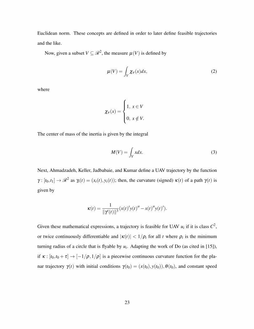
In another study, Ahmadzadeh, Keller, Jadbabaie, and Kumar [15] use an integer pro-
gramming formulation to present a path planning algorithm for multiple fixed-wing UAVs
with body-fixed cameras. To get a sense of how the field of view (FOV) of a UAV camera
is related to its flight path, consider Figures 3 and 4, depicting front and left camera FOVs,
respectively. The work in [15] specifically addresses the cooperative motion planning
problem for heterogeneous UAVs used in surveillance. Each vehicle is modeled as a non-
holonomic point-mass moving at constant speed with minimum turning radius (also known
as Dubin’s car in the literature, as cited in [15]). In the paper, they note that much research
has been conducted concerning multi-UAV task scheduling and planning, but those studies
21
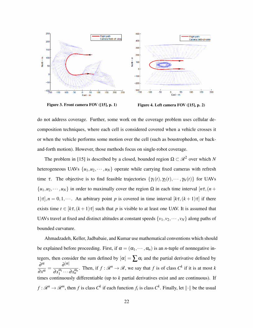
Figure 3. Front camera FOV ([15], p. 1) Figure 4. Left camera FOV ([15], p. 2)
do not address coverage. Further, some work on the coverage problem uses cellular de-
composition techniques, where each cell is considered covered when a vehicle crosses it
or when the vehicle performs some motion over the cell (such as boustrophedon, or back-
and-forth motion). However, those methods focus on single-robot coverage.
The problem in [15] is described by a closed, bounded region Ω ⊂R2 over which N
heterogeneous UAVs u1,u2, · · · ,uN operate while carrying fixed cameras with refresh
time τ . The objective is to find feasible trajectories γ1(t),γ2(t), · · · ,γN(t) for UAVs
u1,u2, · · · ,uN in order to maximally cover the region Ω in each time interval [nτ,(n +
1)τ],n = 0,1, · · · . An arbitrary point p is covered in time interval [kτ,(k + 1)τ] if there
exists time t ∈ [kτ,(k + 1)τ] such that p is visible to at least one UAV. It is assumed that
UAVs travel at fixed and distinct altitudes at constant speeds v1,v2, · · · ,vN along paths of
bounded curvature.
Ahmadzadeh, Keller, Jadbabaie, and Kumar use mathematical conventions which should
be explained before proceeding. First, if α = (α1, · · · ,αn) is an n-tuple of nonnegative in-
tegers, then consider the sum defined by [α] = ∑αi and the partial derivative defined by∂ α
∂xα=
∂ [α]
∂xα11 · · ·∂xαn
n. Then, if f : Rn→R, we say that f is of class Ck if it is at most k
times continuously differentiable (up to k partial derivatives exist and are continuous). If
f : Rn→Rm, then f is class Ck if each function fi is class Ck. Finally, let ‖·‖ be the usual
22
Euclidean norm. These concepts are defined in order to later define feasible trajectories
and the like.
Now, given a subset V ⊆R2, the measure µ(V ) is defined by
µ(V ) =∫
Vχν(x)dx, (2)
where
χν(x) =
1, x ∈V
0, x /∈V.
The center of mass of the inertia is given by the integral
M(V ) =∫
Vxdx. (3)
Next, Ahmadzadeh, Keller, Jadbabaie, and Kumar define a UAV trajectory by the function
γ : [t0, t1]→R2 as γi(t) = (xi(t),yi(t)); then, the curvature (signed) κ(t) of a path γ(t) is
given by
κ(t) =1
‖γ ′(t)‖3 (x(t)′y(t)′′− x(t)′′y(t)′).
Given these mathematical expressions, a trajectory is feasible for UAV ui if it is class C2,
or twice continuously differentiable and |κ(t)| < 1/ρi for all t where ρi is the minimum
turning radius of a circle that is flyable by ui. Adapting the work of Do (as cited in [15]),
if κ : [t0, t0 + τ]→ [−1/ρ,1/ρ] is a piecewise continuous curvature function for the pla-
nar trajectory γ(t) with initial conditions γ(t0) = (x(t0),y(t0)),θ(t0), and constant speed
23
‖γ ′(t)‖= vi, then the parameterized curve γ : [t0, t1]→R2 can be expressed by
γ(t) = (x(t),y(t)),
Thus, the elements needed to completely specify a trajectory γi(t) are the curvature κi(t)
and initial conditions γi(t0) and θi(t0). Using the terminology of calculus, γ(t) is of class
C2 and a flyable trajectory for a UAV with constant velocity v having initial conditions
γ(t0) and θ(t0) with minimum turning radius ρ . Using Do’s work, Ahmadzadeh, Keller,
Jadbabaie, and Kumar were able to change the search space from flyable trajectories γi(t)
to bounded scalar functions κi(t), allowing them to restate their objective as generating
curvature functions κi(t) : |κi(t)| ≤ 1/ρi, i = 1,2, · · · ,N to achieve maximum coverage
for all time intervals [nτ,(n + 1)τ],n = 0,1, · · · .
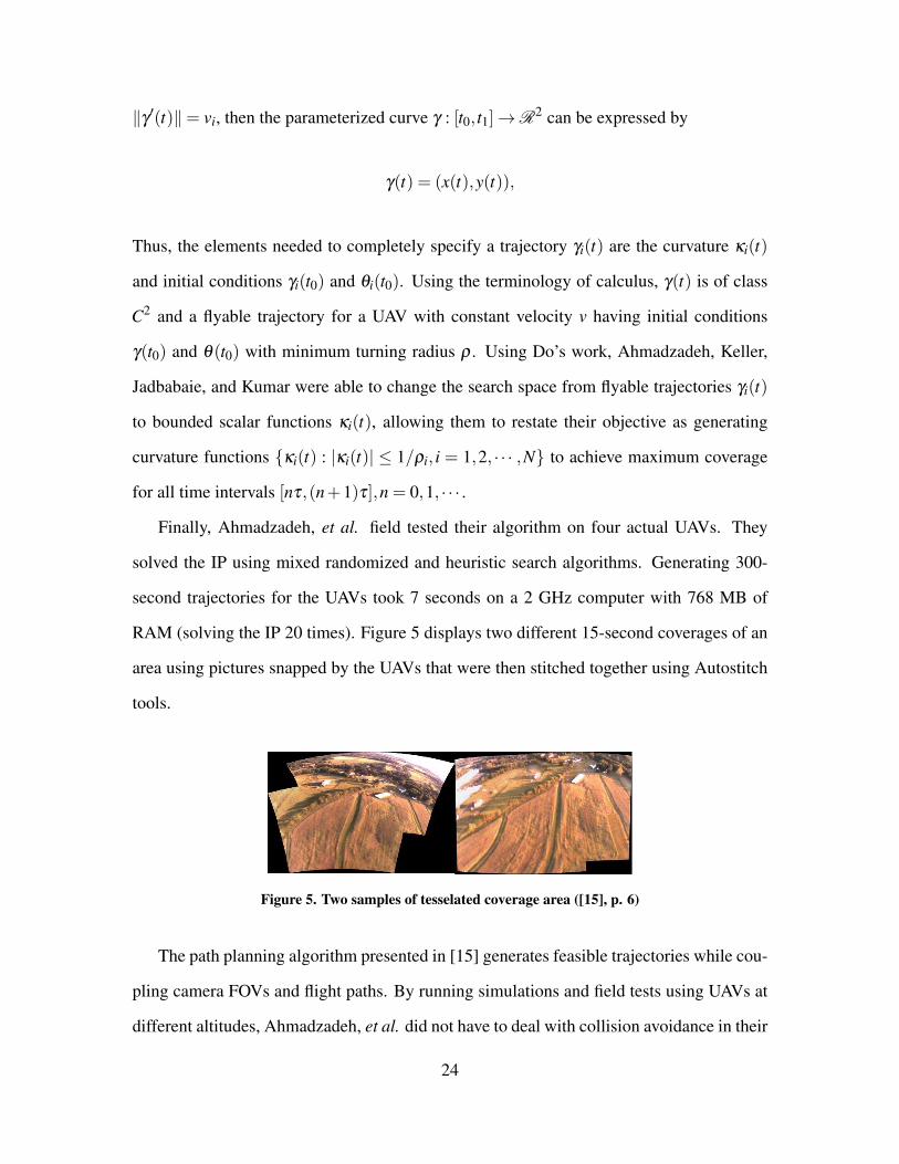
Finally, Ahmadzadeh, et al. field tested their algorithm on four actual UAVs. They
solved the IP using mixed randomized and heuristic search algorithms. Generating 300-
second trajectories for the UAVs took 7 seconds on a 2 GHz computer with 768 MB of
RAM (solving the IP 20 times). Figure 5 displays two different 15-second coverages of an
area using pictures snapped by the UAVs that were then stitched together using Autostitch
tools.
Figure 5. Two samples of tesselated coverage area ([15], p. 6)
The path planning algorithm presented in [15] generates feasible trajectories while cou-
pling camera FOVs and flight paths. By running simulations and field tests using UAVs at
different altitudes, Ahmadzadeh, et al. did not have to deal with collision avoidance in their
24

study. It should also be noted that in their formulation, each part of the area to be covered
had equal priority.
Ousingsawat [36] conducts path planning for a single UAV over a prioritized surveil-
lance space to maximize coverage. The priority of a region of the surveillance space is
modeled using the concept of entropy. Roughly speaking, the more entropy in a region, the
higher its priority. The objective of the planning tool Ousingsawat introduces is to maxi-
mize area coverage in the shortest time while meeting the physical constraints of the UAV
in motion (turning radius, speed, etc.). In terms of entropy, the objective is to plan paths
to reduce entropy as much as possible in minimum time. The paper first describes UAV
dynamics as a hybrid system, then moves on to area and camera footprint parameters, and
finally discusses path generation and simulation results [36].
In hybrid modeling, the system under observation exhibits both continuous and discrete
characteristics. In [36], UAV movements are considered to take place over R2, or, the (x,y)
plane. The UAVs can occupy three possible discrete states xD ∈ 0,1,2; respectively, the
values 0, 1, and 2 indicate going straight, turning left, and turning right. The continuous
states, represented by s = x,y,V,ψ, consist of four variables; (x,y) is location, V is total
velocity, and ψ is UAV heading.
The area under consideration is rectangular. Different regions of the area will be of dif-
fering priorities. Ousingsawat imposes the constraint that the entire area must be explored.
Further, no discontinuities can be admitted as they would result in a non-convex problem,
making it much more difficult to solve. The priorities are assigned using a measure of
entropy, which indicates the uncertainty of a region. In the paper, a boustrophedon search
pattern is assumed and the rectangular area is broken into a grid of cells; as such, each col-
umn of cells has the same entropy (i.e., same priority). Coverage of the area is then defined
by the summation of the entropy in all of the cells. If the grid is N×M, having N rows and
25
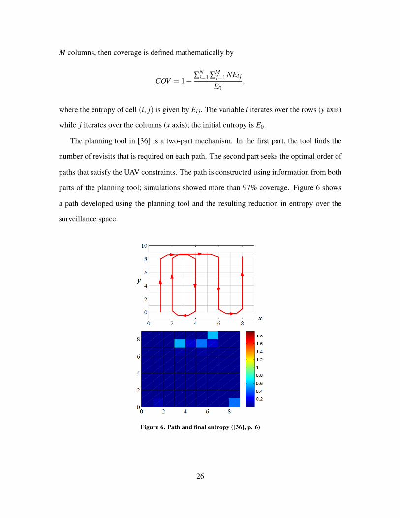
M columns, then coverage is defined mathematically by
COV = 1−∑
Ni=1 ∑
Mj=1 NEi j
E0,
where the entropy of cell (i, j) is given by Ei j. The variable i iterates over the rows (y axis)
while j iterates over the columns (x axis); the initial entropy is E0.
The planning tool in [36] is a two-part mechanism. In the first part, the tool finds the
number of revisits that is required on each path. The second part seeks the optimal order of
paths that satisfy the UAV constraints. The path is constructed using information from both
parts of the planning tool; simulations showed more than 97% coverage. Figure 6 shows
a path developed using the planning tool and the resulting reduction in entropy over the
surveillance space.
Figure 6. Path and final entropy ([36], p. 6)
26
2.2.2 Area Decomposition.
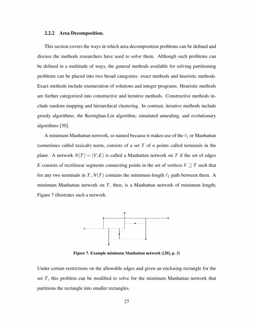
This section covers the ways in which area decomposition problems can be defined and
discuss the methods researchers have used to solve them. Although such problems can
be defined in a multitude of ways, the general methods available for solving partitioning
problems can be placed into two broad categories: exact methods and heuristic methods.
Exact methods include enumeration of solutions and integer programs. Heuristic methods
are further categorized into constructive and iterative methods. Constructive methods in-
clude random mapping and hierarchical clustering. In contrast, iterative methods include
greedy algorithms, the Kernighan-Lin algorithm, simulated annealing, and evolutionary
algorithms [30].
A minimum Manhattan network, so named because it makes use of the `1 or Manhattan
(sometimes called taxicab) norm, consists of a set T of n points called terminals in the
plane. A network N(T ) = (V,E) is called a Manhattan network on T if the set of edges
E consists of rectilinear segments connecting points in the set of vertices V ⊇ T such that
for any two terminals in T , N(T ) contains the minimum-length `1 path between them. A
minimum Manhattan network on T , then, is a Manhattan network of minimum length;
Figure 7 illustrates such a network.
Figure 7. Example minimum Manhattan network ([20], p. 3)
Under certain restrictions on the allowable edges and given an enclosing rectangle for the
set T , this problem can be modified to solve for the minimum Manhattan network that
partitions the rectangle into smaller rectangles.
27

Chepoi, Nouioua, and Vaxes [20] describe a minimum Manhattan network (MMN),
which was introduced by Gudmundsson, Levcopoulos, and Narasimhan [26]. In [20], a
rounding algorithm is proposed based on a linear programming formulation to solve it.
Specifically, they propose and prove correctness of a rounding 2-approximation algorithm
based on an LP-formulation of the MMN. Kato, Imai, and Asano (as cited in [20]) previ-
ously gave such an algorithm, but did not prove correctness.
Choset [21] surveys results in coverage path planning, and in so doing, discusses differ-
ent possible cellular decompositions of a space for efficient robot exploration. He considers
three types of cellular decomposition: approximate, semi-approximate, and exact. In ap-
proximate cellular decomposition, the cells used to decompose an area are the same size
and shape, but the collective area of the cells does not encompass the entire space. Semi-
approximate methods use partial space discretization where the cells have fixed width, but
the tops and bottoms are of arbitrary shape; in a semi-approximate scheme, robots move
along the generated, equal-width columns, recursively exploring the space. Finally, an ex-
act cellular decomposition partitions a search space in the mathematical sense - any two
cells are disjoint and the collection of all cells completely covers the entire space and no
more. Typically, an area that is decomposed exactly is searched using simple back-and-
forth motion by multiple robots.
An example exact cellular decomposition procedure, developed by Choset and Pignon
[22], is boustrophedon cellular decomposition (BCD). In the BCD, a line sweeps an area
generating cells; if any obstacles are present, a cell is divided above and below the obstacle
and recombined to form a single cell after passing the obstacle. Traditionally, exact cellular
decompositions have been used for two purposes. Those purposes are either to deal with
obstacles in an environment or to divide a target space over multiple vehicles [33].
Carlsson [18] presents a type of equitable partition that decomposes an area where
vehicles are routed through a collection of depots such that each vehicle receives a fair
28

share of the workload. Carlsson gives an algorithm that takes as input a planar, simply-
connected region R that has defined on it a probability density function f . The region R
contains n depot points P = p1, p2, · · · , pn that represent starting locations of n vehicles.
It is assumed that the points each correspond to exactly one vehicle. Though client locations
are unknown, they are assumed to be independent and identically distributed according to
the probability density function f . The goal is to partition R into n subregions with one
vehicle assigned to each member of the partition. If large samples are drawn, the workload
in each subregion is asymptotically equal. Carlsson shows that the problem is solved by
treating each subregion Ri as a traveling salesman problem (TSP) with a set of points that
includes the depot and all points in Ri. The problem is easily visualized in Figure 8.
Figure 8. (a) Depot set and density function f ; (b) Area partitioned; (c) Points sampled independentlyof f ; (d) TSP tours of each subregion asymptotically equal ([18], p. 2)
As Carlsson shows, the situation here is a special case of the equitable partitioning
problem. In that class of problems, a pair of densities f1 and f2 is defined on a region R. The
partitioning of R must be such that∫∫
Ri
f1 dA =1n
∫∫R
f1 dA and∫∫
Ri
f2 dA =1n
∫∫R
f2 dA
29

for all i, where one density represents the set of depots and the other the TSP workload over
a subregion when points are sampled from f . Now, it is possible to simply induce a partition
by using vertical lines across an area, but that might not give the best solution in the end.
Further constraints are imposed; a natural constraint to consider is that each subregion Ri
should include the depot assigned to it (and only that one depot). Another important factor
is the shape of the region to be divided. If R is convex, each region Ri may be required to
also be convex. However, in the case where R is nonconvex, relative convexity is desired
among all subregions. That is, the shortest path between two points u and v in Ri for the ith
subregion must be contained in Ri. An interesting visual example of the algorithm applied
to a real-world map is presented in Figure 9.
Figure 9. (a) Hennepin County, MN with locations of 29 largest post offices; (b) Equitable partition:same population ( [18], p. 17)
30

Maza and Ollero [31] apply polygon area decomposition to a convex area R with no
holes or obstacles that must be searched. In their work, a team of heterogeneous UAVs is
to search an area of land for objects of interest such as fires, cars, property damage, etc.
Initially, each UAV being used is situated on an edge of the polygon search area as shown
in Figure 10.
Figure 10. Polygon with vertices Vi and UAVs at starting positions Si ([31], p. 3)
Beginning this way, Maza and Ollero build on the anchored area partition problem
presented by Hert and Lumelsky [28], who employ a semi-approximate cellular decompo-
sition. Now, if S1,S2, · · · ,Sn is a set of starting positions for n UAVs and if P is the area of
the entire region (and Pi the area of each partitioned subregion), then each UAV has an area
requirement, denoted AreaRequired(Si), specifying the desired area of each subregion Pi.
Then, a polygon P containing q sites (called a q-site polygon) is termed area-complete if
AreaRequired(S(P)) = Area(P). The expression AreaRequired(S(P)) represents the sum
of the areas required by all sites in P. Citing [28], Maza and Ollero explain that the desired
area partition can be accomplished using n− 1 line segments. Each line divides a q-site
area-complete polygon into two convex polygons, one of which is q1-site area-complete
and the other q2-site area-complete. The area partition algorithm can be repeated n− 1
times to yield n convex 1-site area-complete polygons.
31
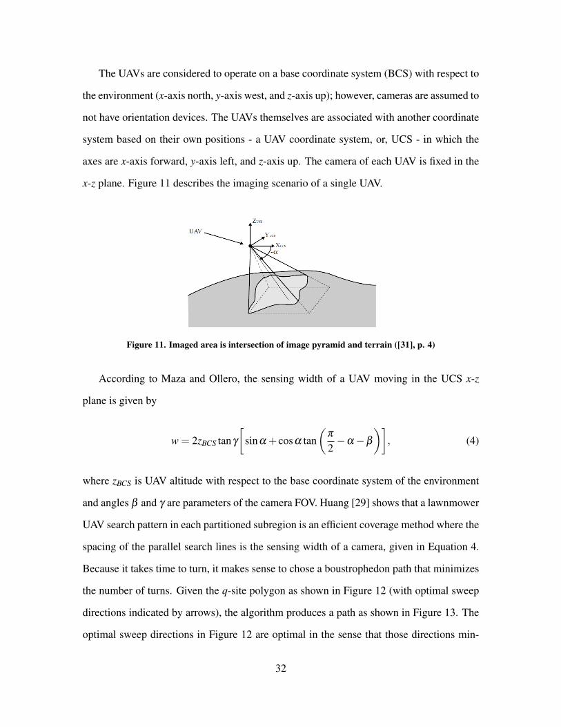
The UAVs are considered to operate on a base coordinate system (BCS) with respect to
the environment (x-axis north, y-axis west, and z-axis up); however, cameras are assumed to
not have orientation devices. The UAVs themselves are associated with another coordinate
system based on their own positions - a UAV coordinate system, or, UCS - in which the
axes are x-axis forward, y-axis left, and z-axis up. The camera of each UAV is fixed in the
x-z plane. Figure 11 describes the imaging scenario of a single UAV.
Figure 11. Imaged area is intersection of image pyramid and terrain ([31], p. 4)
According to Maza and Ollero, the sensing width of a UAV moving in the UCS x-z
plane is given by
w = 2zBCS tanγ
[sinα + cosα tan
(π
2−α−β
)], (4)
where zBCS is UAV altitude with respect to the base coordinate system of the environment
and angles β and γ are parameters of the camera FOV. Huang [29] shows that a lawnmower
UAV search pattern in each partitioned subregion is an efficient coverage method where the
spacing of the parallel search lines is the sensing width of a camera, given in Equation 4.
Because it takes time to turn, it makes sense to chose a boustrophedon path that minimizes
the number of turns. Given the q-site polygon as shown in Figure 12 (with optimal sweep
directions indicated by arrows), the algorithm produces a path as shown in Figure 13. The
optimal sweep directions in Figure 12 are optimal in the sense that those directions min-
32

imize the assigned polygon’s diameter along the sweep direction. Note, only directions
perpendicular to edges need to be tested.
Figure 12. Area partition ([31], p. 8) Figure 13. lawnmower pattern search ([31], p. 8)
Another way to break down a space for exploration by machines is to use grid decompo-
sition, or an occupancy grid map (OGM) representation of the space. Quijano and Garrido
[38] explore two possible grid decompositions. One decomposition uses a hexagonal grid
and the other a quadrangular grid. Figure 14 illustrates the difference.
Figure 14. Hexagonal and Quadrangular Grid Decomposition over same map ([38], p. 2)
Quijano and Garrido note that because the diagonal and vertical (or horizontal) distances
between square centers in a quadrangular decomposition are different (diagonal of a square
is larger than any side by a factor of√
2), managing different distances and scales for the
purpose of robot exploration can add complexity to the problem. In that case, in order to
33
simplify the process of exploring the space, one can restrict robot movement to only vertical
and horizontal movements. In the case of a hexagonal decomposition, this is not a problem
because the vertical, horizontal, and diagonal distances between centers of hexagons are
the same.
Quijano and Garrido [38] find that though a map may be represented by both the
hexagonal and quadrangular grid decompositions, the space can be better represented using
hexagons rather than squares even if the resolution is enhanced in both cases. If the space
is small, then the choice of decomposition is superfluous. Four different algorithms are
developed in [38] to search a space once it has been decomposed into both hexagons and
squares. The exploration algorithms are versions of well-known graph search algorithm
types: breadth-first, breadth-first random, depth-first, and best-first. When they applied
their algorithms to each decomposition of the same map, what they found was that the
variance in the number of movements required by robots searching the map was lower
in the hexagonal case than in the quadrangular case. The overall number of movements
required in the hexagonal cases was also lower than in the quadrangular setup. Similar re-
sults applied when the space contained obstacles, except in that situation, the initial starting
position of robots was key to the number of movements needed for robots to explore the
space.
Nigam and Kroo [34] conducted work specifically on the persistent surveillance prob-
lem using decomposition techniques. In their study, they look at the coverage of an area
of land using multiple UAVs. The authors start with a semi-heuristic control policy for
a single UAV and extend that approach to the case of multiple UAVs. They perform this
extension in two ways. The first is to extend a reactive policy for a single UAV (each UAV
reacts to the environment and other UAVs on its own) to multiple UAVs and the second
is to partition the surveillance space and then allocate a UAV to each member of the par-
tition for parallel surveillance. The assignment of UAVs to subregions of the surveillance
34

space is based on auction algorithms. Nigam and Kroo compare the two ways to extend the
single-UAV policy, noting interesting results.
In the case of an area divided into two cells that must be continuously monitored by
a single UAV, suppose that the UAV can only choose to do one of two actions: go left
or go right. Then, the optimal policy is decided by its first action, as after the UAV has
decided initially to go left or right, in order to have continuous coverage of the area, it must
alternatively go left and right, shuttling between the two cells. This simplified single-UAV
persistent coverage scenario in [34] is depicted in Figure 15.
Figure 15. Simplified two-cell persistent coverage problem ([34], p. 2)
The figure requires some explanation.
Each cell has an associated age, given by T1 and T2; these times represent the time
elapsed since cell 1 and cell 2 were last observed, respectively. The UAV is initially located
a distance x from the left cell and is traveling at velocity Vsurvey. If the distance between
cells 1 and 2 is 1 unit (x and Vsurvey scaled accordingly), then initially, the UAV is 1− x
units from cell 2. Nigam and Kroo seek a UAV policy to minimize the maximum age over
both cells. In this case, that policy simplifies to determining which way to go first, left or
right. If T1 is taken to be less then T2 (without loss of generality), then age graphs can be
constructed for both the case where the UAV goes left first and for when the UAV goes
right first; these graphs comprise Figures 16 and 17, respectively. In these figures, the
optimal policy is the one that minimizes the peak of the maximum age curve (in black in
both figures). Because the optimal policy is determined after the first move, the planning
horizon is finite for the total possible distance traveled to visit both cells of 2/Vsurvey.
35

Figure 16. Age of cells, left first ([34], p. 3) Figure 17. Age of cells, right first ([34], p. 3)
Nigam and Kroo show that the cell with the greatest value is the critical cell because the
concern here is only with the maximum age recorded, thus, when extending the 1-D single-
UAV example to a 1-D example with five cells, the optimal policy is to choose the cell of
maximum value - the target cell - and take the maximum step toward it. This method, a
target-based approach, is in contrast to a sum-of-values approach in which the UAV moves
toward the area with the highest sum of values of cells (by linearly combining cell ages
and distances from the UAV). If two cells are of equal value, then the cell that requires the
least heading change becomes the target cell. The researchers use the weight parameter
−1/Vsurvey five-cell setup as in the two-cell situation, but they caution that such a weight
may not be optimal for the multiple cell case in general. The weight parameter is derived
using an iterative sampling (ISIS) based optimizer. The optimal policy results in a spiral
search pattern for a square surveillance space.
After comparing various approaches to the single-UAV case (different direction-finding
methods), Nigam and Kroo move on to the multiple UAV case. The two methods re-
searchers use to treat the multiple-UAV problem are a multi-agent reactive policy (ex-
tension of the single-UAV policy) and space decomposition (optimally partitioning, and
searching the space in parallel using one UAV per partitioned subregion). Here, only the
SD approach is considered. It should be noted, however, that for a large enough num-
36
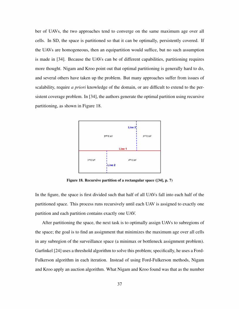
ber of UAVs, the two approaches tend to converge on the same maximum age over all
cells. In SD, the space is partitioned so that it can be optimally, persistently covered. If
the UAVs are homogeneous, then an equipartition would suffice, but no such assumption
is made in [34]. Because the UAVs can be of different capabilities, partitioning requires
more thought. Nigam and Kroo point out that optimal partitioning is generally hard to do,
and several others have taken up the problem. But many approaches suffer from issues of
scalability, require a priori knowledge of the domain, or are difficult to extend to the per-
sistent coverage problem. In [34], the authors generate the optimal partition using recursive
partitioning, as shown in Figure 18.
Figure 18. Recursive partition of a rectangular space ([34], p. 7)
In the figure, the space is first divided such that half of all UAVs fall into each half of the
partitioned space. This process runs recursively until each UAV is assigned to exactly one
partition and each partition contains exactly one UAV.
After partitioning the space, the next task is to optimally assign UAVs to subregions of
the space; the goal is to find an assignment that minimizes the maximum age over all cells
in any subregion of the surveillance space (a minimax or bottleneck assignment problem).
Garfinkel [24] uses a threshold algorithm to solve this problem; specifically, he uses a Ford-
Fulkerson algorithm in each iteration. Instead of using Ford-Fulkerson methods, Nigam
and Kroo apply an auction algorithm. What Nigam and Kroo found was that as the number
37

of UAVs increased, the MRP and SD methods resulted in increasingly similar performance
in terms of maximum age over all cells in the space. However, the performance of both
methods with respect to the lower bound on the optimal maximum age decreased, due
possibly to more congestion in the area or restriction to rectangular partitions.
Nigam and Kroo also consider what effect UAV dynamics have on performance. As-
suming UAVs travel at constant velocity and constant altitude, they find that a simulation
ignoring turn rates and moments is suitable. Instead, minimum turning radius is instrumen-
tal in defining the minimum distance between one cell of the space and another. When a
UAV has to travel from a point A to another point B, to find the minimum length trajectory,
the lengths of four paths between the points - as illustrated in Figure 19 - are calculated,
and the minimum-length path is chosen.
Figure 19. Possible optimal paths from A to B ([34], p. 11)
Two types of distance could be used to define a policy for UAV trajectories, a Euclidean
distance policy (EDP) or an actual distance policy (ADP). The Euclidean distance is the
straight line distance from A to B, whereas the actual distance accounts for the total distance
traveled by a UAV as it executes turns and flies in its characteristic fashion from one point
to another. What Nigam and Kroo discovered is that the ADP policy will result in better
performance than an EDP policy. Table 2 summarizes the average (of fifty trials) maximum
ages recorded using actual and Euclidean distance policies.
38
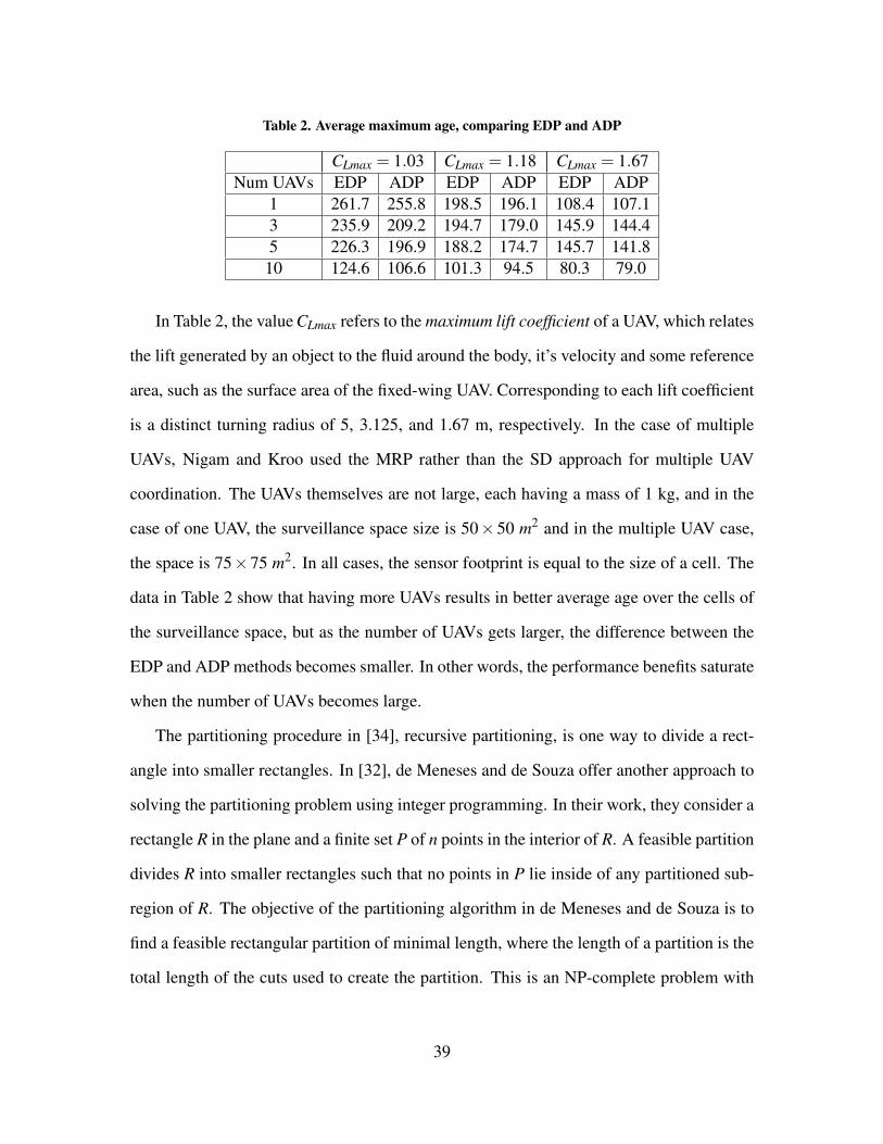
Table 2. Average maximum age, comparing EDP and ADP
CLmax = 1.03 CLmax = 1.18 CLmax = 1.67Num UAVs EDP ADP EDP ADP EDP ADP
1 261.7 255.8 198.5 196.1 108.4 107.13 235.9 209.2 194.7 179.0 145.9 144.45 226.3 196.9 188.2 174.7 145.7 141.810 124.6 106.6 101.3 94.5 80.3 79.0
In Table 2, the value CLmax refers to the maximum lift coefficient of a UAV, which relates
the lift generated by an object to the fluid around the body, it’s velocity and some reference
area, such as the surface area of the fixed-wing UAV. Corresponding to each lift coefficient
is a distinct turning radius of 5, 3.125, and 1.67 m, respectively. In the case of multiple
UAVs, Nigam and Kroo used the MRP rather than the SD approach for multiple UAV
coordination. The UAVs themselves are not large, each having a mass of 1 kg, and in the
case of one UAV, the surveillance space size is 50× 50 m2 and in the multiple UAV case,
the space is 75×75 m2. In all cases, the sensor footprint is equal to the size of a cell. The
data in Table 2 show that having more UAVs results in better average age over the cells of
the surveillance space, but as the number of UAVs gets larger, the difference between the
EDP and ADP methods becomes smaller. In other words, the performance benefits saturate
when the number of UAVs becomes large.
The partitioning procedure in [34], recursive partitioning, is one way to divide a rect-
angle into smaller rectangles. In [32], de Meneses and de Souza offer another approach to
solving the partitioning problem using integer programming. In their work, they consider a
rectangle R in the plane and a finite set P of n points in the interior of R. A feasible partition
divides R into smaller rectangles such that no points in P lie inside of any partitioned sub-
region of R. The objective of the partitioning algorithm in de Meneses and de Souza is to
find a feasible rectangular partition of minimal length, where the length of a partition is the
total length of the cuts used to create the partition. This is an NP-complete problem with
39

applications in very large-scale integration design. Figure 20 shows a rectangle with points
inside, a non-guillotine partition, and a guillotine partition. The RGP term used to describe
Figure 20(a) refers to the class of problems defined by rectangles with interior points or
“holes.”
Figure 20. (a) Instance of RGP (b) Non-guillotine partition (c) Guillotine partition ([32], p. 6)
Note that in Figure 20, the optimal partition is not the guillotine partition. In computa-
tional experiments, de Meneses and de Souza found that a guillotine partition never solved
the problem exactly. When the points are completely noncorectilinear (no two points be-
long to the same horizontal or vertical line), as is the case with the RGP in Figure 20, the
complexity of the problem increases.
De Meneses and de Souza discuss the many approximate algorithms in the literature
that have been used to solve this problem; they range in complexity from O(n logn) to
O(n5). A rectangle with points inside is called an RGP, and an instance of the RGP is
I = (R,P), where R and P are a rectangle and a set of points, respectively. A grid is defined
in [32] by the set of straight vertical and horizontal lines intersecting at the points inside R
(belonging to P). Such a grid is called the grid induced by P, and is denoted GI(P). Points
in P are called terminal points, or more simply, terminals. Those points at intersections of
horizontal and vertical lines of GI(P) that are not in P are called Steiner points. Figure 21
shows both grid points and Steiner points. De Meneses and de Souza reason that an optimal
solution S∗ to I = (R,P) consists of straight lines that lie on the grid GI(P).
40

Figure 21. Terminal points (black), Steiner points (white), and GI(P) (dotted lines) ([32], p. 7)
To solve the problem, de Meneses and de Souza set up an IP in two ways. The first is
the segment model and the second is the set partitioning model. The first step in making
this a 0− 1 integer programming problem using the segment model is deciding whether
each grid segment is part of an optimal solution. Any resulting optimal solution cannot
include knees or islands. A knee is defined as a terminal or Steiner point where exactly two
grid segments meet at a right angle, and an island exists when only one segment is incident
on a terminal or Steiner point. Figure 22 illustrates a knee and an island.
Figure 22. (a) a knee and (b) an island at a terminal point ([32], p. 7)
If knees or islands are admitted, then it is not possible to produce a partition of the space
where each subregion is a rectangle. In fact, the absence of knees and islands serves as a
necessary condition for a subset C ⊆GI(P) of grid segments to form a feasible rectangular
partition of R with respect to P. What de Meneses and de Souza show is that given an in-
41

stance I = (R,P) of the RGP, only when every terminal point in P has at least two segments
of C incident to it does C induce a feasible rectangular partition of R with respect to P.
Proceeding from these observations, de Meneses and de Souza construct a 0− 1 IP as
follows. For each grid segment e ∈ GI(P),
xe =
1, if e belongs to a solution S
0, otherwise.
Letting |GI(P)| = m, an m-dimensional binary vector x characterizes a solution. Because
the objective is to find a minimum-length partition, the length of each segment is needed.
If the length of every segment of GI(P) is captured in the vector d ∈ Rm, where the eth
component of d is the length of segment e in GI(P), then the objective is to minimize dTe xe.
Expressed another way, the objective is to minimizem
∑e=1
dexe.
Each grid point i may connect up to four grid segments. If those segments are denoted
i(1), i(2), i(3), and i(4), then, in order to achieve a feasible solution, there must be cer-
tain constraints on the terminal and Steiner points. Combining these constraints with the
objective function, the IP formulation follows (for each point in GI(P)).
Minimizem
∑e=1
dexe
subject to
xi(1) + xi(2) ≥ 1
xi(1) + xi(4) ≥ 1
xi(3) + xi(2) ≥ 1
xi(3) + xi(4) ≥ 1
xi(1) + xi(2)− xi(3) ≥ 0
42

xi(1) + xi(2)− xi(4) ≥ 0
xi(1) + xi(4)− xi(2) ≥ 0
xi(1) + xi(4)− xi(3) ≥ 0
xi(3) + xi(2)− xi(1) ≥ 0
xi(3) + xi(2)− xi(4) ≥ 0
xi(3) + xi(4)− xi(1) ≥ 0
xi(3) + xi(4)− xi(2) ≥ 0
0≤ x≤ 1
x integer
The first four constraints avoid knees and islands at terminal points and the next four avoid
them at Steiner points. Clearly, if |P| is large, then the IP formulation will be very large
as well, as this formulation above would essentially be multiplied in size by the number of
points. The authors prove that a vector xS ∈ Rm is part of a feasible rectangular partition S
if and only if xS satisfies all terminal and Steiner point constraints.
In the set partitioning model, to solve the problem of finding the minimum-length par-
tition of a rectangle R, de Meneses and de Souza start with the standard set partitioning
problem. That is, given a set H = 1, · · · ,m and the set K = K1, · · · ,Kn of subsets of
H (the power set of H), if J = 1, · · · ,n, then the set J∗ ⊆ J is called a partition of H if
∪ j∈J∗K j = H and for all j, l ∈ J∗ where j 6= l, we have K j∩Kl = ∅ (dividing H into mutu-
ally exclusive and collectively exhaustive subsets of H). To each subset K j ∈ K, a cost c j is
associated, and the goal of the integer program here, to find the minimum-length partition
of R, is then given by the IP formulation
Minimizen
∑j=1
c jy j
43
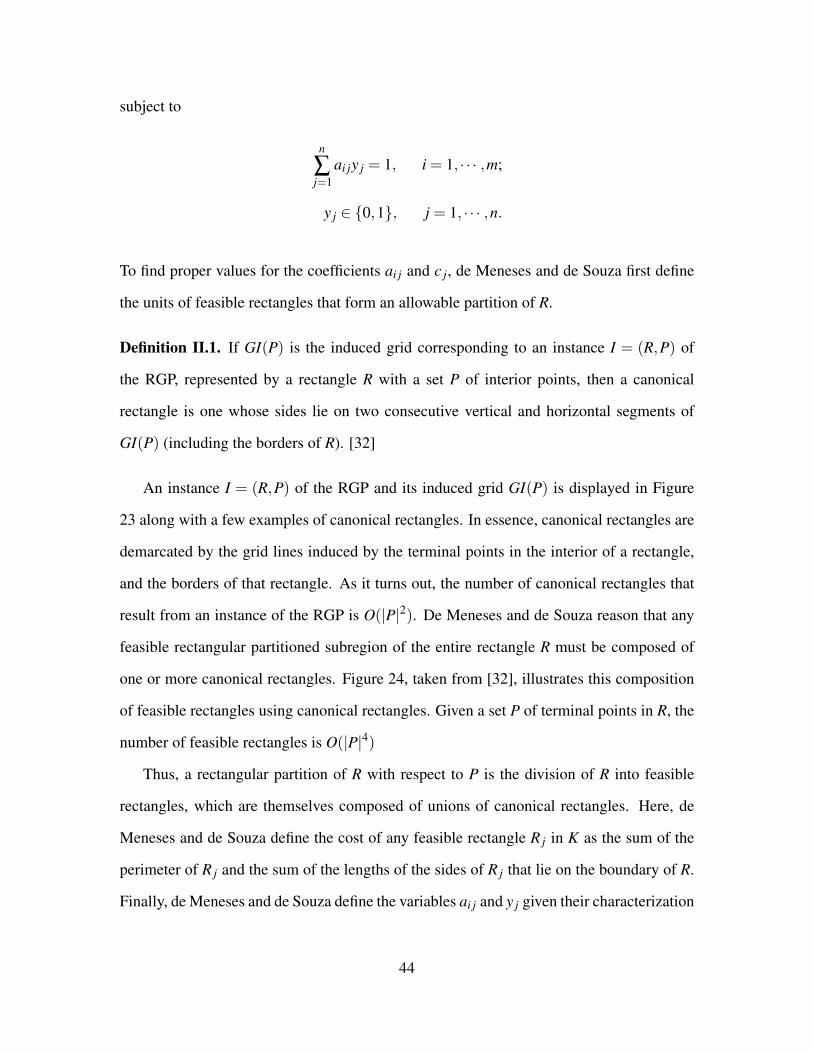
subject to
n
∑j=1
ai jy j = 1, i = 1, · · · ,m;
y j ∈ 0,1, j = 1, · · · ,n.
To find proper values for the coefficients ai j and c j, de Meneses and de Souza first define
the units of feasible rectangles that form an allowable partition of R.
Definition II.1. If GI(P) is the induced grid corresponding to an instance I = (R,P) of
the RGP, represented by a rectangle R with a set P of interior points, then a canonical
rectangle is one whose sides lie on two consecutive vertical and horizontal segments of
GI(P) (including the borders of R). [32]
An instance I = (R,P) of the RGP and its induced grid GI(P) is displayed in Figure
23 along with a few examples of canonical rectangles. In essence, canonical rectangles are
demarcated by the grid lines induced by the terminal points in the interior of a rectangle,
and the borders of that rectangle. As it turns out, the number of canonical rectangles that
result from an instance of the RGP is O(|P|2). De Meneses and de Souza reason that any
feasible rectangular partitioned subregion of the entire rectangle R must be composed of
one or more canonical rectangles. Figure 24, taken from [32], illustrates this composition
of feasible rectangles using canonical rectangles. Given a set P of terminal points in R, the
number of feasible rectangles is O(|P|4)
Thus, a rectangular partition of R with respect to P is the division of R into feasible
rectangles, which are themselves composed of unions of canonical rectangles. Here, de
Meneses and de Souza define the cost of any feasible rectangle R j in K as the sum of the
perimeter of R j and the sum of the lengths of the sides of R j that lie on the boundary of R.
Finally, de Meneses and de Souza define the variables ai j and y j given their characterization
44
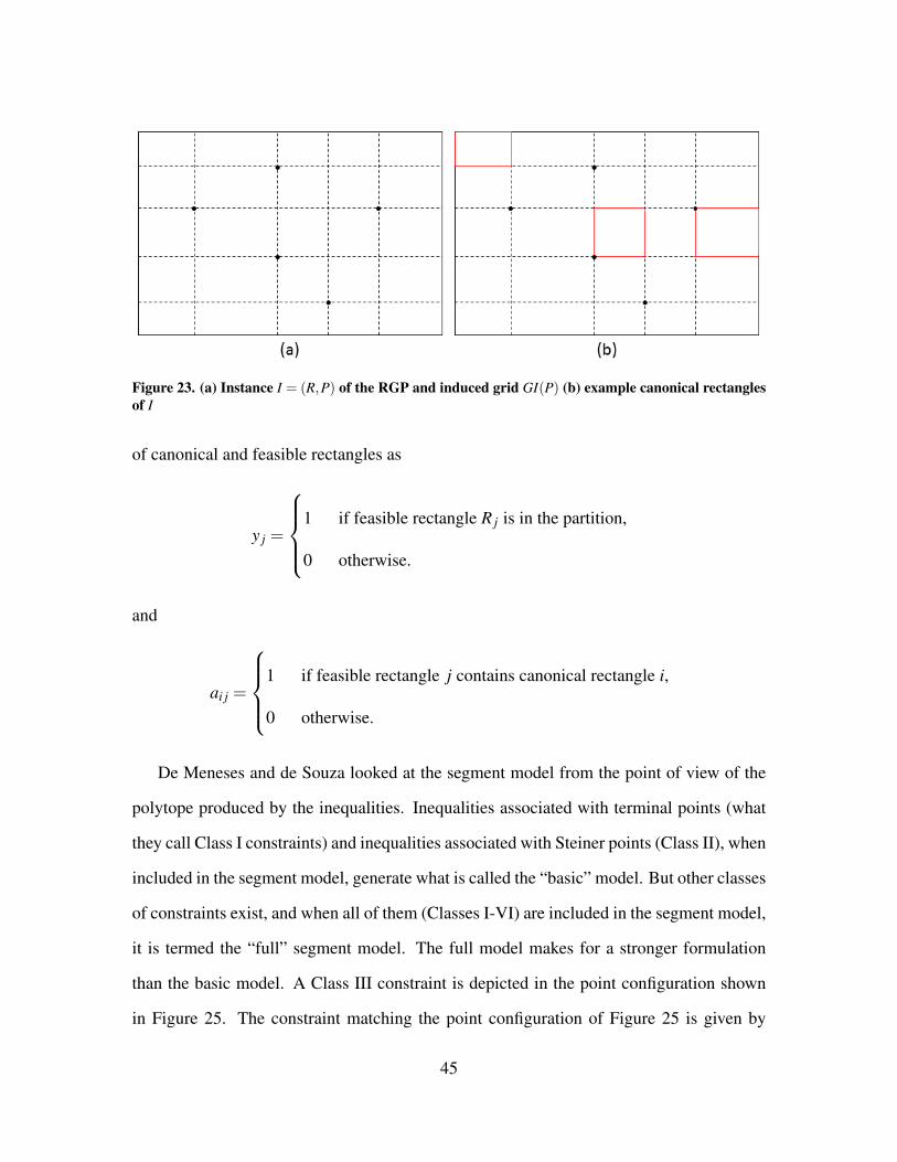
Figure 23. (a) Instance I = (R,P) of the RGP and induced grid GI(P) (b) example canonical rectanglesof I
of canonical and feasible rectangles as
y j =
1 if feasible rectangle R j is in the partition,
0 otherwise.
and
ai j =
1 if feasible rectangle j contains canonical rectangle i,
0 otherwise.
De Meneses and de Souza looked at the segment model from the point of view of the
polytope produced by the inequalities. Inequalities associated with terminal points (what
they call Class I constraints) and inequalities associated with Steiner points (Class II), when
included in the segment model, generate what is called the “basic” model. But other classes
of constraints exist, and when all of them (Classes I-VI) are included in the segment model,
it is termed the “full” segment model. The full model makes for a stronger formulation
than the basic model. A Class III constraint is depicted in the point configuration shown
in Figure 25. The constraint matching the point configuration of Figure 25 is given by
45

Figure 24. RGP is 2×2 square with P consisting of centroid of square. Four canonical rectangles result.Canonical rectangles A and B comprise feasible rectangle E and canonical B and C make up feasible G.([32], p. 23)
x1 + x2 + x3 + x4 ≥ 2, and there are O(n) such constraints, where n is the number of points
in the interior of R (terminal plus Steiner points).
Figure 25. Point configuration of a Class III constraint ([32], p. 17)
These Class III inequalities define facets of PR, the polytope given by the convex hull
of the integer solutions of the formulation given for the segment model. De Meneses and de
Souza further show that PR = convxs ∈Rm : S is a rectangular partition of R with respect to P,
where m = |GI(P)| = dim(PR). That is, the polytope PR is full-dimensional. The other
classes of inequalities, Classes IV-VI, correspond to point configurations shown in Figure
26, taken from [32]. With the exception of Class IV inequalities, they all define facets of
46

PR without qualification. A Class IV inequality, however, defines a facet of PR if and only
if in the point configuration for the inequality - shown in Figure 26(a) - both pairs of points
(p2, p3) and (p4, p5) contain at least one Steiner point.
Figure 26. Point configuration: (a) Class IV Inequality, x1 + x2 + x3 + x4 ≥ 1; (b) Class V Inequality,
28
∑i=1
xi +12
∑i=9
xi−14
∑i=13
xi ≥ 6; (c) Class VI Inequality,8
∑i=1
xi ≥ 2 ([32], pp. 18-21)
Denoting the segment model formulation in [32] by FS and the set partition model by
FR, what de Meneses and de Souza found was that the second formulation is stronger. They
determined this by comparing the bounds obtained by solving the linear relaxation of FR
with those of FS and proving that if W ∗ represents the optimal value of the linear relaxation
of FR and Z∗ that of FS for a given instance of the RGP, then W ∗ ≥ 2Z∗+ 2Per(R), where
Per(R) is the perimeter of R. Moreover the inequality is not necessarily satisfied at equality.
Based on computational experiments, de Meneses and de Souza found that in the seg-
ment model, the branch-and-bound algorithm performed better than the branch-and-cut al-
gorithm. In the set partitioning model, the researchers implemented a branch-and-price al-
gorithm; they found that the better quality of the set partitioning bounds makes the branch-
and-price algorithm more efficient than the branch-and-bound segment model. When the
best known approximate algorithm is applied to each instance of the RGP tested, on av-
erage, the approximate solution was 10% off the optimum; worse, it never converged on
47

the optimal value. With high noncorectilinearity, the difficulty of using these algorithms
increases.
2.3 Summary
There are a number of ways to define the coverage problem for a region given a set of
UAVs. Certainly, there are coverage problems involving single-UAV scenarios, multiple
homogeneous UAVs, multiple heterogeneous UAVs, continuous coverage, persistent cov-
erage, coverage for the sake of searching a space once with minimal overlap, and more.
Further, the methods used to solve these types of problems are just as numerous. Some
techniques that have been used involve integer programming, using scheduling theory, ap-
plying the concept of entropy to define percentage of area covered, genetic algorithms,
heuristics, dynamic programming, and others. A common overarching approach to the
coverage problem in general - although it is not absolutely necessary - is to first decompose
the area to be surveyed into subregions or cells and then to assign UAVs to surveil each cell
separately. Decomposition of a space is often a hard problem, and most researchers make
some simplifying assumptions to make the problem either tractable or at least solvable in a
reasonable amount of time given the application.
Of the models discussed in this chapter, the one that was selected for the methodology
of this research is the model provided by de Meneses and de Souza. In the next chapter,
surveillance spaces that contain points of interest are modeled as rectangles with holes, or
instances of the RGP. The RGPs are then divided into smaller, non-overlapping rectangles
using a set partitioning model that is solved by a 0-1 integer program. Furthermore, the
algorithm used to assign UAVs from a set of available vehicles to the partitioned subregions
of the surveillance space is also described. The assignment algorithm seeks to minimize
the revisit times over each member of the partition of the space by assigning the appropriate
UAV to each subregion.
48

III. Methodology
3.1 Introduction
This chapter describes the methodology used to set up and solve the persistent surveil-
lance problem given the assumptions set out in Chapter I. The chapter is divided into several
sections. In the first two sections, the surveillance space partitioning and UAV assignment
processes are explained in detail. The third section uses a flow chart to give a high-level
summary of the process of randomly generating operational scenarios and solving them,
and the final section presents the operational scenarios that are actually solved, the results
and analysis of which appear in Chapter IV.
3.2 Surveillance Space Partitioning
The general approach taken in this research to solve the persistent surveillance prob-
lem is to divide or partition an area into subregions and then to assign exactly one UAV
per region (to conduct surveillance on the whole area). Consider terrain where there exist
a number of locations that must be monitored from a military intelligence point of view.
For example, one might be the house where a suspected enemy combatant lives. Another
location could be a suspected meeting place, where high-level members of a terrorist or-
ganization have been known to congregate. There are many possibilities. Sometimes, it is
necessary to collect intelligence on not only these locations but the areas surrounding them.
For instance, being able to track the individuals traveling to and from a meeting place can
provide a source of valuable intelligence that can help military analysts understand human
relationships, movements and actions, and other information that can be used to determine
what is happening on the ground. Through this kind of intelligence gathering, it is possible
to catch individuals planting explosive devices. It also becomes easier in this case to dis-
49
cover what associations individuals have with other individuals, possibly known criminals
or terrorist suspects.
A persistent surveillance program executed over the area can help uncover what is hap-
pening on the ground and what human relationships exist between actors of interest to
military intelligence. Regard the area of interest as a two-dimensional map and suppose
there are “interesting ” locations on that map. Around the set of locations, a rectangle is
drawn. Then, identify with each location a point so as to maximize corectilinearity. These
points are terminal points. Next, construct the grid induced by these terminal points over
the map, which produces some Steiner points. For partitioning the rectangle, two main
goals have been explored in the context of partitioning rectilinear polygons (such as rectan-
gles): (1) minimizing the number of rectangles, and (2) minimizing the total length of the
cut segments required to produce the rectangles. Because the rectangle has interior points
that need to be considered (called “holes” in the literature), the problem is NP-complete
[35]. The goal here is the first - to minimize the number of rectangles that result from
partitioning R. It is necessary to mathematically express this desire as the objective of the
IP. A feasible partition must have all cuts forming the partition pass through at least one
terminal point, and each terminal point must lie on a cut. After partitioning the space, the
resulting number of subregions must be minimal because exactly one UAV will be assigned
to each region. If the number of regions produced by the partitioning algorithm is minimal,
then the number of UAVs needed to carry out the persistent surveillance program is also
minimal. Figure 27 describes the process of generating a grid from a set of locations and
what an optimal partition might look like if the objective is to minimize partition length. In
this case, the partition also minimizes the number of rectangles.
Let Figure 27(b) represent an instance, I of the RGP, where the outside rectangle is R
and the set of three terminal points is P. That is, I = (R,P) is an instance of the RGP, a
rectangle R with a set P of interior terminal points. Figure 27(c) also shows GI(P), the
50

Figure 27. (a) Locations of interest (b) Introducing terminal points (c) Induced grid with 3 terminalpoints and 3 Steiner points (d) Notional minimal partition
grid induced by the set P, which reveals three Steiner points. To minimize the partition
length, segment model in [32] can be used. In that case, to formulate an IP for this prob-
lem, the segments and points of the RGP need to be indexed. Then, a vector ~d ∈ R17
defines the length of each segment in GI(P). Suppose that the dimensions of R are 20 units
by 14 units, and further, that each segment of GI(P) is indexed left to right, then top to
bottom (horizontal segments, then vertical). The terminal and Steiner points are indexed
together going left to right from the top row to the bottom. Using such an indexing, let
~d = (5,6,5,4,5,6,5,4,5,5,4,5,5,4,5,5,4), where the ith component of ~d is the length of
the ith segment of GI(P). A solution to this problem is another vector of decision variable
values (0 or 1), ~x ∈ R17. The objective is to minimize 〈~d,~x〉, and the constraints on grid
points are exactly as given in [32], multiplied over three terminal and three Steiner points.
51

Note that the solution exhibited in Figure 27(d) is expressed by the vector of decision vari-
ables,~x = (1,1,1,1,0,0,0,0,0,0,0,0,1,1,0,0,0).
In a real-world case, represent an area can be represented as a rectangle and a set of
interesting locations inside of the rectangle using points that maximize corectilinearity.
But there may be more than one way to place points on structures (one per structure) such
that the points maximize being in horizontal and vertical lines. Figure 28 depicts a set of
buildings and some possible configurations for the set of terminal points P.
Figure 28. (a) Maximum corectilinearity of P (b) Alternative with maximum corectilinearity of P
Thus, consider an instance of the RGP wherein the set P might not be fixed. Suppose, that
is, that we have a set of locations - buildings, perhaps - in an area we wish to survey using
UAVs. Then, we can model each location as a point. But where on each building do we
place the point? The centroid of the building outline on a 2-D map seems like a natural
candidate for a terminal point. However, doing that might not maximize corectilinearity
among the terminal points. Thus, we can consider different configurations for the set P and
then find the minimum-length partition of each configuration, take the minimum overall
and make that partition the output of the process.
However, the objective is the partition that results in the smallest number of rectangles.
To that end, a conjecture is stated about the minimum-rectangle partition of the RGP, given
52

that the set P can vary in some sense. When the set P is not fixed, we call P variable and
denote it as Pv, and consider the RGP a variable RGP (VRGP); this is really a set of RGPs,
one instance per set Pv. Let LR,Pv be the length of any partition of R given the set of terminal
points Pv. Then, the conjecture is stated as follows.
Conjecture 1 Given an instance of the VRGP, I = (R,Pv), a minimum-length partition
divides R into the minimum number of rectangles. Furthermore, the absolute minimum-
length partition is of length min
minPv
LR,Pv
.
Now, if the surveillance space is quite large, say, on the order of tens of square kilometers,
then the VRGP could essentially be modeled as an ordinary RGP by choosing the terminal
points to coincide with centers of mass relative to surrounding structures of interest from
an intelligence perspective. To motivate Conjecture 1, it holds true in the case of Figure
27(d). Consider another example in Figure 29, where there are five areas of interest, to each
of which is assigned a point such that corectilinearity is maximized. There can be at most
two pairs of corectilinear points in this case; note that in each of the scenarios in Figure
27(b)-(f), there are two pairs of corectilinear points (Corectilinearity is maximized in every
case.). Figure 27(f) shows the minimum length partition, which yields the smallest number
of rectangles. It is important to observe here that where the terminal point is placed on each
location can vary, and that choice results in a different set of possible cuts.
If the interior points are completely noncorectilinear, as in Figure 30, then there is little
concern about the placement of points within locations as no vertical or horizontal line
passes through any two locations simultaneously. As a result, the point on each location can
be chosen to be the centroid of the location. Now, observe a necessary (but not sufficient)
condition to ensure the cuts generate the minimum-length partition: for any pair of points
on a vertical or horizontal grid line, a single cut must pass through them in order to achieve
the minimum-length partition of the rectangle, which, by conjecture, results in the smallest
53
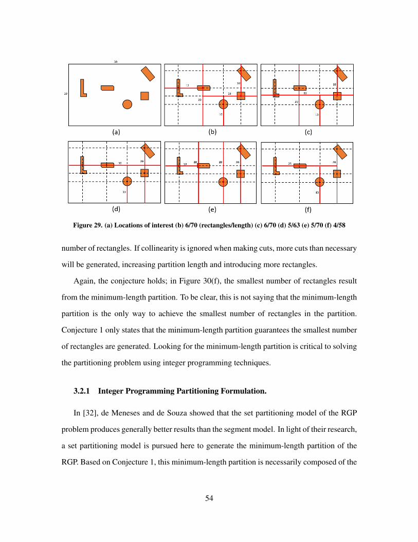
Figure 29. (a) Locations of interest (b) 6/70 (rectangles/length) (c) 6/70 (d) 5/63 (e) 5/70 (f) 4/58
number of rectangles. If collinearity is ignored when making cuts, more cuts than necessary
will be generated, increasing partition length and introducing more rectangles.
Again, the conjecture holds; in Figure 30(f), the smallest number of rectangles result
from the minimum-length partition. To be clear, this is not saying that the minimum-length
partition is the only way to achieve the smallest number of rectangles in the partition.
Conjecture 1 only states that the minimum-length partition guarantees the smallest number
of rectangles are generated. Looking for the minimum-length partition is critical to solving
the partitioning problem using integer programming techniques.
3.2.1 Integer Programming Partitioning Formulation.
In [32], de Meneses and de Souza showed that the set partitioning model of the RGP
problem produces generally better results than the segment model. In light of their research,
a set partitioning model is pursued here to generate the minimum-length partition of the
RGP. Based on Conjecture 1, this minimum-length partition is necessarily composed of the
54

Figure 30. (a) Locations of interest (b) 4/60 (rectangles/length) (c) 4/55 (d) 5/65 (e) 4/51 (f) 4/50
minimum number of rectangles. Because a set partitioning model is used, the length of the
partition is related to the perimeters of the rectangles included in the partition.
Consider the four operational scenarios in Figure 31, modeled as instances of the RGP.
In each part of Figure 31, the ordered pair associated with each terminal point in the RGP is
each point’s coordinates, given that (0,0) corresponds to the lower left corner of rectangle
R. All rectangles in Figure 31 are of size 40 km×50 km. Next, for each rectangle Ri, we
draw GI(Pi) in Figure 32.
The standard set partitioning problem presented in Chapter 2 was:
Minimizen
∑j=1
c jy j
subject to
n
∑j=1
ai jy j = 1, i = 1, · · · ,m;
y j ∈ 0,1, j = 1, · · · ,n.
55

Figure 31. (a) I1 = (R1,P1) ; (b) I2 = (R2,P2) ; (c) I3 = (R3,P3) ; (d) I4 = (R4,P4)
In [32], the cost of each feasible rectangle was its perimeter plus the lengths of the sides
coincident with the sides of R. However, when implementing the set partitioning model, a
simpler cost structure resulted in the same optimal solution as the cost structure presented
by de Meneses and de Souza. In fact, setting the cost of each rectangle to its perimeter
resulted in the same minimal cost as that achieved using the cost function described by de
Meneses and de Souza.
Each instance of the RGP is encoded as a list of points (x and y coordinates) corre-
sponding to the intersections of segments of GI(P) (terminal and Steiner points) and those
points on the borders of R that intersect segments of GI(P). These points are entered into a
56
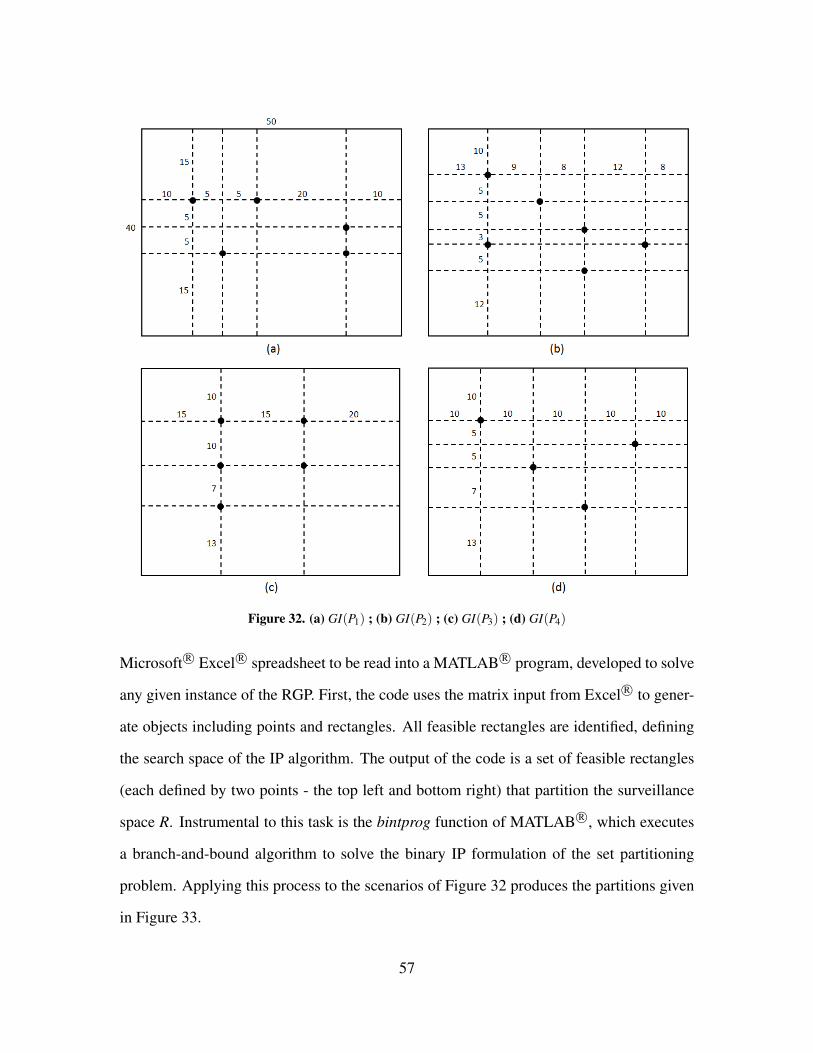
Figure 32. (a) GI(P1) ; (b) GI(P2) ; (c) GI(P3) ; (d) GI(P4)
Microsoft R© Excel R© spreadsheet to be read into a MATLAB R© program, developed to solve
any given instance of the RGP. First, the code uses the matrix input from Excel R© to gener-
ate objects including points and rectangles. All feasible rectangles are identified, defining
the search space of the IP algorithm. The output of the code is a set of feasible rectangles
(each defined by two points - the top left and bottom right) that partition the surveillance
space R. Instrumental to this task is the bintprog function of MATLAB R©, which executes
a branch-and-bound algorithm to solve the binary IP formulation of the set partitioning
problem. Applying this process to the scenarios of Figure 32 produces the partitions given
in Figure 33.
57

Figure 33. (a) I1 solved ; (b) I2 ; (c) I3 ; (d) I4
3.3 UAV Assignment
Once the surveillance space is partitioned, consider the task of assigning exactly one
UAV to each member of the partition, Part(R). The objective is to assign the appropriate
UAV to each member Part(R). In order to do that, the flight pattern of the UAVs needs
to be considered. It takes a significant amount of time for an aircraft to execute a coordi-
nated turn. In fact, Huang [29] points out that the number of turns a UAV needs to make
while conducting a survey is the main factor in the cost difference between different sweep
directions. As a consequence, if minimal revisit time is desired, a reasonable expectation
58

for a persistent surveillance program, UAV paths that minimize the number of turns are
required. Moreover, Maza and Ollero [31] explain that simulations show back-and-forth,
or boustrophedon motion, to be more efficient than a spiral pattern. All this amounts to
stating that it is more efficient for a UAV to sweep a rectangle by moving back and forth
parallel to the longest side of that rectangle.
Also consider the size of each member of Part(R). For a small region, it makes more
sense to assign a smaller UAV to it, capable of making tight turns, rather than, say, a
larger aircraft with a greater maximum speed, which is better suited for larger members of
Part(R). As such, the partitioning algorithm is progressive in the sense that the minimally-
capable UAV is assigned to a given region such that the maximum revisit time desired by
a decision maker is respected. This also ensures parsimony in terms of the types of UAVs
delivered to an area of operations. For example, if an RQ-11 Raven can meet a decision
maker’s needs, then it makes sense to order that UAV to the field rather than the more
expensive RQ-7 Shadow to do the same job. Other considerations that are important when
considering how to assign UAVs to regions of the space include the time it takes to deliver
a system to the theater, how many of a particular airframe are in the inventory, UAV fuel
type, means of takeoff, ceiling, payload capacity, etc. All of these concerns are important
factors in determining which type of UAV should be assigned to each member of Part(R).
For example, if JP-8 fuel is scarce in a particular area of operations but gasoline is plentiful,
then it might make sense to assign a gasoline-powered UAV instead of one that uses JP-8,
if both systems are otherwise comparable and could appropriately be assigned to the same
member of Part(R).
Still other considerations important to the assignment process include personnel issues
such as deployment tempo of UAV operators, the type and amount of equipment that needs
to be delivered along with UAVs to an area of operations, UAV susceptibility to jamming
or attack, vehicle reliability and maintainability, and the logistics of returning UAVs to the
59

United States from a theater after operations have been completed. If a UAV is delivered
to theater because it can cover an area in a manner consistent with a decision maker’s
surveillance plans, but it is not very maintainable given the circumstances, then perhaps a
different UAV would have been a better choice. Thinking about these issues before deciding
on a particular UAV for a given region can reduce waste in terms of time and money by
delivering the right system at the right time.
Although the number of UAVs operated by the departments of the United States Gov-
ernment, including the military services, the NSA, CIA, and others is large, here the UAV
assignment problem is simplified by restricting the available UAVs to a subset of all UAVs
available for military (surveillance only) use. To better understand the class of vehicles
from which a set may be selected to perform persistent surveillance, the general classes of
UAVs are presented in Figure 34.
Figure 34. UAV categories ([5], p. 9)
Thus, given a partitioned surveillance space, UAVs are chosen generally from one of these
categories. If, for example, the partitioned space includes both a 5 km× 2 km rectangle
and a 50 km× 15 km rectangle, and the mission timeline is on the order of a few hours,
then it makes sense to include both a mini UAV and a tactical UAV in any air package sent
60

to surveil the space persistently. On the other hand, if a member of the partition of R is
150 km× 75 km and the mission timeline is on the order of days, then a strategic UAV
such as the RQ-4 Global Hawk should perhaps be included in the UAV package.
This research assumes that the UAVs that are available to use in a persistent surveillance
program are those identified in Figure 34, namely, the RQ-11 Raven, RQ-7 Shadow, and
the RQ-4 Global Hawk. To decide which one to use for a given member of Part(R), the
flight and camera swath characteristics of each vehicle are needed. These are estimated in
Table 3.
Table 3. UAV characteristics: Global Hawk, Shadow, and Raven
UAV Cruise Speed (km/h) Camera Swath (km)RQ-4 Global Hawk 640 10
RQ-7 Shadow 185 3RQ-11 Raven 48 1
Given this information, along with the dimensions of Part(R), and a decision maker’s de-
sired maximum revisit time for the locations identified by the intelligence community, the
output produced is the best UAV of the three options for each subregion of R - the one
that optimizes (minimizes) revisit times to terminal points along the path of a UAVs sweep
within each subregion. The system diagram shown in Figure 35 depicts the inputs and
output of this assignment process.
The assignment process requires some explanation. Suppose E ⊂ Part(R) is of height
h and width w. Figure 36 helps to develop the formula for the estimated maximum revisit
time test to a terminal point associated with a UAV sweeping the region in a lawnmower
pattern. Part (a) of Figure 36 is a case where E has a width that is less than or equal to the
width of the camera swath s of one of the UAVs that could be selected to sweep that region
(such as an RQ-11 Raven). If a Raven is chosen to sweep this area, then it can sweep the
entire area and visit point p = (x,y) in one pass. Depending on where p is along the height
of E, the maximum revisit time will vary.
61

Figure 35. UAV assignment process for any E ⊂Part(R) given UAVs A (RQ-4), B (RQ-7), and C (RQ-11).
Assume for the moment that y > h− y. In that case, if the UAV is traveling from the
bottom of the rectangle to the top, then first observes point p in t1 = y/vC hours. It then
revisits point p on the return sweep toward the bottom of E in t2 = 1/60 + 2(h− y)/vC
hours, assuming that a 180 turn takes one minute to execute. Then the vehicle revisits p
once more in t3 = 1/60+2y/vC hours as it passes the point while moving toward the bottom
and returns to the point, traversing a distance of 2y km while traveling at the cruising speed,
vC km/h. The estimated maximum revisit time to point p, if a Raven is chosen to conduct
the surveillance, is then given by test = maxt2, t3. Following this calculation of test , the
subset of the available UAVs that satisfy test ≤ tmax (where tmax is a decision maker’s desired
maximum revisit time) is identified, and the element of this subset with the minimum value
(the best UAV) is assigned to survey E.
62

Figure 36. (a) Case: w≤ s; (b) Case: w > s
If E looks more like the rectangle in Figure 36(b), where the UAV sensor swath may
have less size than the height of E, then the time it takes for some UAV initially traveling
in a left-to-right direction from top to bottom, say UAV A, to revisit point p after its initial
visit in t1 = x/vA hours is
tLR2 = [2(w− x)+ 2wh/s]/vA + 2h/s + 1/60.
Returning to p at this point takes the UAV t3 = 1/60 + 2x/vA hours, which is relatively
small. On the fourth visit, t4 = t2. The UAV repeats this process until the end of the
mission timeline. The maximum revisit time in this scenario becomes tLRest = tLR
2 , where LR
indicates the left-to-right initial direction of the UAV’s motion. The situation changes if the
UAV initially sweeps in a right-to-left pattern instead of moving left-to-right at the outset.
When this happens, the maximum revisit time occurs on the second pass as well, and
tRLest = [2x + 2wh/s]/vA + 2h/s + 1/60
63

hours. Because UAV operators have control over the initial direction of flight (right-to-left
or left-to-right) the initial direction can be chosen to be that which minimizes the estimated
revisit time, test = mintLRest , t
RLest . These calculations depend on the UAV continuously
retracing its path going from the top to bottom of R; that is, whatever path it follows as it
sweeps to the bottom of the rectangle, it retraces on the return trip. Thus, the overall path
of a UAV is determined by its initial sweep of the surveillance space.
3.4 Partitioning and Assignment Flowchart
Figure 37 summarizes in a flowchart the high-level process of randomly generating a
surveillance space (an instance of the RGP), dividing the space into smaller rectangles, and
then assigning the appropriate UAV to each smaller rectangle. The details of this imple-
mentation, that is, the pseudocode used to produce the output, are located in Appendices B
and C.
Figure 37. High-level depiction of partitioning and assignment process
64

3.5 Operational Scenarios
Having developed the code to solve instances of the RGP using MATLAB R©, the next
step was to write code using Microsoft R© Excel R© Visual Basic for Applications (VBA)
to generate scenarios as random instances of the RGP. The inputs to that process are the
number of desired terminal points and the dimensions of the surveillance space. Without
loss of generality, the terminal points are spaced apart from the edges of the rectangular
surveillance area. Each scenario is detailed in Figures 38-39; for these cases, they are
presented as pure instances of the RGP. However, they could just as easily have come from
a map with Global Positioning Satellite coordinates. In the next chapter, the process of
partitioning a space and assigning UAVs to the partition is implemented by applying that
process to each operational scenario in Figures 38-39.
3.6 Summary
In this chapter, the process used to partition a space based on an IP formulation method-
ology provided in [32] is outlined. Further, the algorithms used to decide which UAV to
assign to each member of the partitioned space from a pool of available UAVs is also de-
scribed as a way to assign the minimally-capable UAV to each subregion of a partitioned
space, reducing waste in spending. Finally, the entire process is summarized in a single
flowchart to better understand the end-to-end method for creating a persistent surveillance
program over a rectangular surveillance space, which is modeled as an instance of the RGP.
65

Figure 38. Scenarios: Set I
66
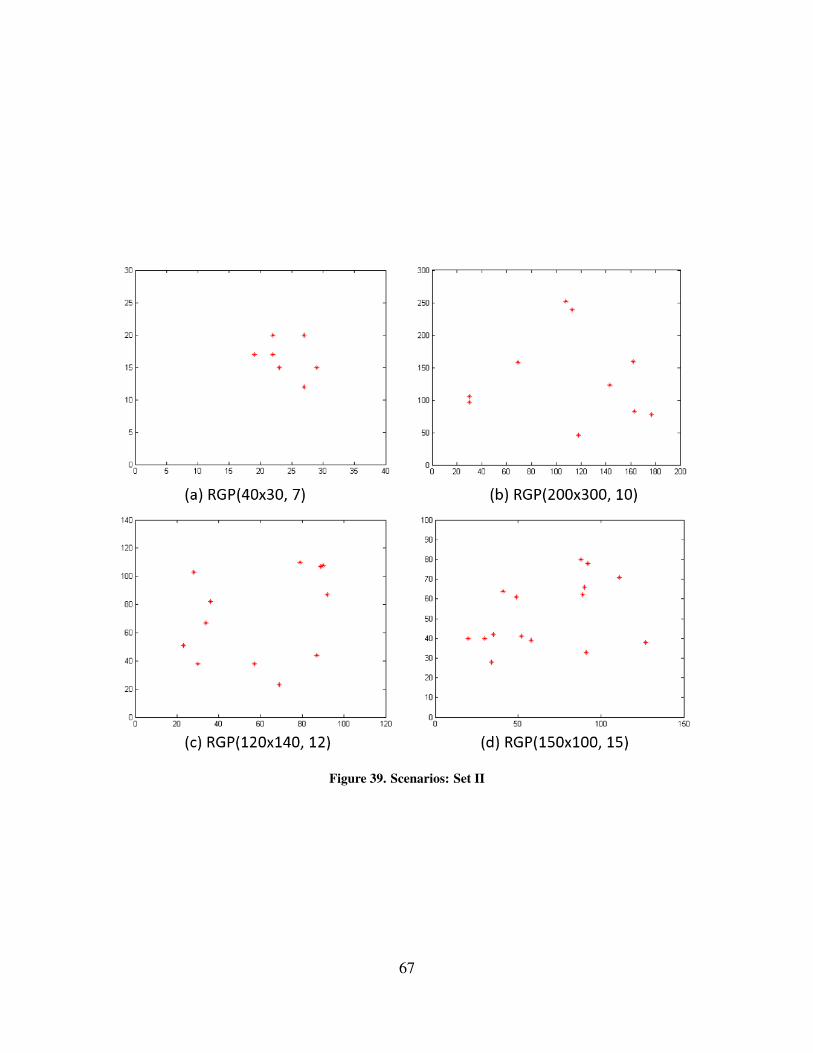
Figure 39. Scenarios: Set II
67

IV. Implementation and Analysis
4.1 Introduction
In this chapter, the algorithms developed in Chapter 3 for partitioning a surveillance
space based on the work of [32] and assigning exactly one UAV to each member of the
partition are implemented to solve operational persistent surveillance scenarios. This is
followed by an analysis of the results and a discussion on the insights and limitations asso-
ciated with the approach used here. Finally, this chapter concludes with a brief description
of the logistics of moving UAVs into an area of operations.
4.2 Implementation
The solutions to the scenarios of Set I are presented as partitions of the associated RGP
instances in Figure 40. Within each member of the partition of each surveillance space, the
appropriately assigned UAV is indicated. Figure 41 presents the solutions to the scenarios
in Set II.
Each solution is accompanied by the RGP parameters and the maximum revisit time in
hours over all subregions based on their assigned UAVs. For example, in Figure 40(b), the
dimensions of the surveillance space are 60× 50 km and the number of terminal points is
5. In addition, the maximum revisit time over any partitioned subregion is 5 hours.
One quantity not displayed in Figures 40 and 41 is the mission timeline. The reason for
this omission is that the mission timeline only dictates how often UAVs over a partitioned
subregion must be swapped based on UAV endurance. For example, if the scenario depicted
in Figure 40(b) has a mission timeline of 48 hours, then in region 1 (top left rectangle),
UAV operators would need to swap the operating RQ-7 Shadow, which has an endurance
of six hours, for a fresh vehicle a total of eight times over the course of 48 hours. This
is precisely why a minimum of two and UAVs are required for each region. It is better,
68

however, to have a minimum of three UAVs on hand (if available) for each region. In that
case, one is in operation, one is in maintenance mode, and the third is a spare. Thus, for the
300 km2 rectangle in Figure 40(b), having 12 RQ-7 Shadow UAVs and three RQ-11 UAVs
on hand would ensure continuous execution of the persistent surveillance program on that
space.
Figure 40. Solutions to scenarios in Set I
69

Figure 41. Solutions to scenarios in Set II
4.3 Analysis
4.3.1 Partitioning and Assignment.
Knowing the maximum revisit time of each cell gives more information about the de-
composed surveillance space to a decision maker. With this level of detail, a decision
maker can manage expectations of a surveillance program. The decision maker can effec-
tively communicate to authorities and imagery customers the level of surveillance that can
be obtained using a parsimonious number of UAVs of the correct types for the surveillance
mission. Beyond simply being able to communicate what can be achieved by a surveillance
program of this type, the decision maker can reduce waste in spending by ordering only the
70

correct types of UAVs in the correct numbers. It makes little sense to request an RQ-4
Global Hawk, a very expensive UAV with extensive support equipment, when two or three
RQ-7 Shadow UAVs might suffice for a particular surveillance mission.
Although it makes good sense to have on hand three UAVs for each subregion under
surveillance, the actual number that need to be on hand is a matter of UAV reliability and
maintainability, which is outside the scope of this research. Furthermore, on the battlefield,
a decision maker such as a military commander is afforded flexibility in making decisions
about how to execute the surveillance program to include how many UAVs need to be
requested for a given surveillance program. Modifications to the solution presented by
the algorithm in this research are expected, making the output of the process implemented
here a good starting point for a persistent surveillance program that can be adapted to any
specific need in theater.
In particular, ordering more or less than the minimum number of UAVs (as projected
by the algorithm presented in this research) of a given type for a particular subregion is
an option for a commander. If the commander decides that current intelligence is more
accurate than previous estimates, and that a region may not be important enough to surveil,
the commander can opt to apply resources elsewhere. On the other hand, if a comman-
der is not satisfied with the revisit time (desiring a shorter revisit time interval) that can
be expected from the mapping of UAVs to subregions as described in this research, then
the commander can order more of that particular type of UAV, or even replace that type
with a more capable UAV; switch an RQ-11 for an RQ-7, for example. Without a starting
point, however, the task of deciding how to partition the surveillance space and deciding
which UAV should be assigned to each subregion to meet revisit time expectations is more
difficult. With the algorithm given in this research, the task becomes simpler and can be
finished more quickly.
71

The partitioning algorithm presented in this research works well for medium-sized
problems, measured in terms of the number of feasible rectangles generated by the RGP.
For scenarios involving up to 15 terminal points (which generate a number of feasible rect-
angles), the algorithm quickly provides an optimal solution, but including more terminal
points generates increasingly many feasible rectangles, and the output tends to become un-
reliable. In some cases, when the number of terminal points approaches or exceeds 20, no
feasible solution is produced by the algorithm. Thus, a limitation of the process to solve
the persistent surveillance problem is that it does not work well for larger problems.
The reason for this limitation is that unlike a linear program (LP), which is a continuous
optimization problem, an IP (a discrete optimization problem) has no general optimality
conditions. Thus, even though the solution space of a general IP may be quite small in
comparison to the solution space of an LP, solving the IP can take a long time and require
great effort, whereas very large LPs can be solved often much more simply using general
techniques with little difficulty using modern software [39]. Thus, various methods have
evolved over time to solve IPs. These methods fall into three categories, namely, enumer-
ation techniques (a class that includes branch-and-bound, the method used by the bintprog
function in MATLAB R©), cutting-plane techniques, and group-theoretic techniques [25].
The focus here is on branch-and-bound, as it was used to solve the problems posed in this
research.
When the bintprog function is called in MATLAB R© to solve a problem formulated as an
IP, the function uses an LP-based branch-and-bound algorithm to produce a solution. The
algorithm employed in MATLAB R© relaxes the binary constraint on the decision variables
x, allowing 0 ≤ x ≤ 1. This procedure works by searching for a binary integer feasible
solution, updating the best integer point found by the current iteration, and verifying that
no better integer feasible solution is possible by solving a series of LPs [11]. Typically,
using the default options of bintprog, the algorithm terminates, finding no feasible solution
72
for larger problems. However, an operational scenario of the type studied in this research
is not likely to include large numbers of points that need to be observed for a long period
of time. If that does become the case, then grouping points in clusters and identifying each
cluster as a single terminal point (at the cluster centroid) can help reduce the dimensionality
of the problem.
The most time-consuming part of solving an IP is verification of optimality. Once a
solution is reached, it must be verified as being optimal, and to do that, the algorithm must
check the solution against a number of other candidate solutions. For integer programs,
even small problems can result in a large space in which to search during optimality verifi-
cation. This is sometimes referred to as “combinatorial explosion.” In those cases, solving
an IP to optimality becomes very difficult, if not impossible, and one is forced to resort to
heuristic methods that do not guarantee optimality [39]. The fact that bintprog implements
a branch-and-bound algorithm, an exact solution method, means that it is limited in the
size of problem it is capable of solving given any particular hardware on which a solution
is attempted.
In their research, de Meneses and de Souza used a branch-and-price algorithm to solve
their IP-formulated partitioning problem, comparing its performance to the best known ap-
proximate method of solution. A branch-and-price algorithm is a variation on the branch-
and-bound algorithm (branch-and-bound implemented by MATLAB R© in bintprog func-
tion) in which column generation is allowed. This means that at each node of the search
tree generated by a branch-and-bound algorithm, columns may be generated to tighten the
bounds on the LP-relaxation at that stage. Branch-and-price is used to solve large-scale
IPs, and it is complementary to cutting in the branch-and-cut algorithm, which involves
row generation [16]. It is possible that larger partitioning problems - larger than those rep-
resented by the operational scenarios in this research - could be solved more readily using
a branch-and-price algorithm.
73
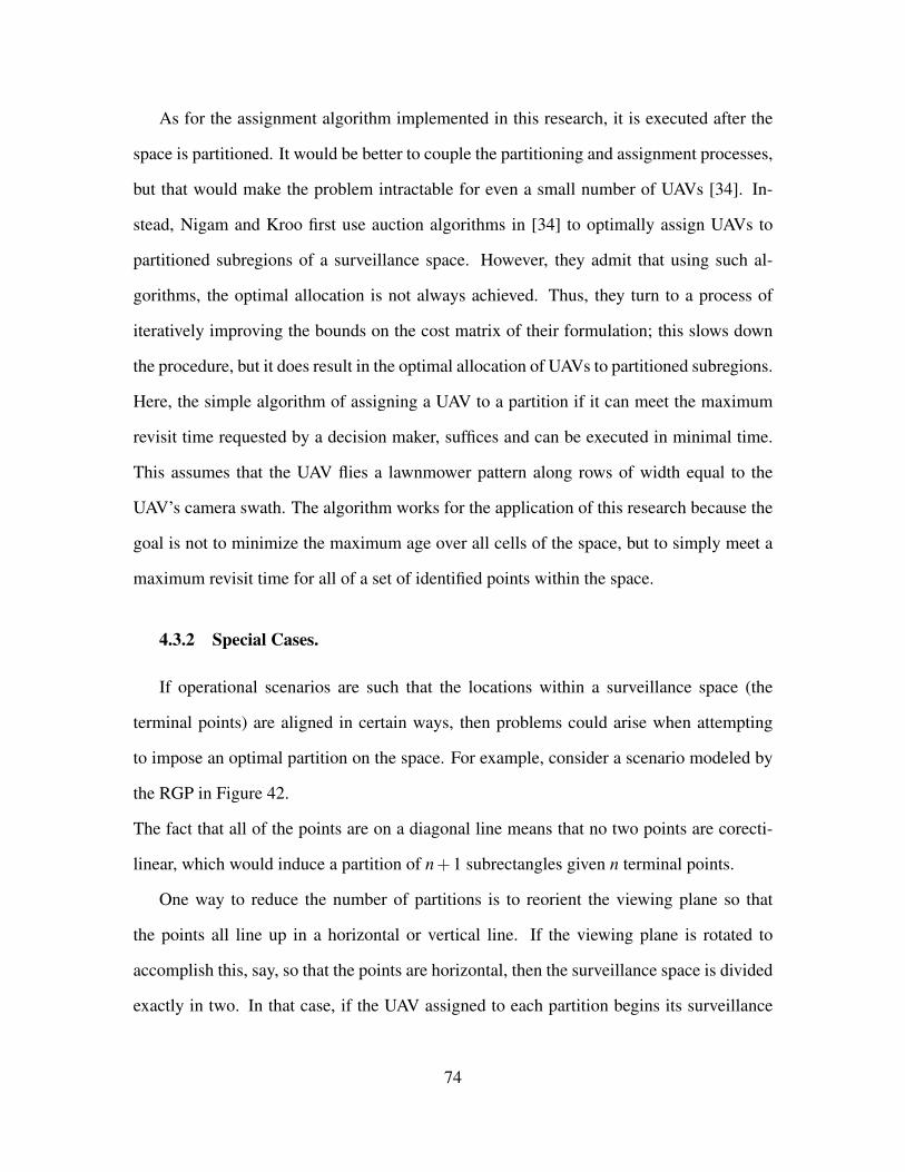
As for the assignment algorithm implemented in this research, it is executed after the
space is partitioned. It would be better to couple the partitioning and assignment processes,
but that would make the problem intractable for even a small number of UAVs [34]. In-
stead, Nigam and Kroo first use auction algorithms in [34] to optimally assign UAVs to
partitioned subregions of a surveillance space. However, they admit that using such al-
gorithms, the optimal allocation is not always achieved. Thus, they turn to a process of
iteratively improving the bounds on the cost matrix of their formulation; this slows down
the procedure, but it does result in the optimal allocation of UAVs to partitioned subregions.
Here, the simple algorithm of assigning a UAV to a partition if it can meet the maximum
revisit time requested by a decision maker, suffices and can be executed in minimal time.
This assumes that the UAV flies a lawnmower pattern along rows of width equal to the
UAV’s camera swath. The algorithm works for the application of this research because the
goal is not to minimize the maximum age over all cells of the space, but to simply meet a
maximum revisit time for all of a set of identified points within the space.
4.3.2 Special Cases.
If operational scenarios are such that the locations within a surveillance space (the
terminal points) are aligned in certain ways, then problems could arise when attempting
to impose an optimal partition on the space. For example, consider a scenario modeled by
the RGP in Figure 42.
The fact that all of the points are on a diagonal line means that no two points are corecti-
linear, which would induce a partition of n + 1 subrectangles given n terminal points.
One way to reduce the number of partitions is to reorient the viewing plane so that
the points all line up in a horizontal or vertical line. If the viewing plane is rotated to
accomplish this, say, so that the points are horizontal, then the surveillance space is divided
exactly in two. In that case, if the UAV assigned to each partition begins its surveillance
74

Figure 42. All points diagonally collinear
sweep on the bottom edge of its assigned region, then the revisit time for the line of points
is equal to the time needed for a UAV to sweep its rectangle once because by the time the
top region is swept, the UAV in the bottom region will have reached the line of points. On
the return trips, the top UAV will have revisited the line of points. This pattern continues
over the mission timeline.
The action of orienting a space so as to maximize corectilinearity can be considered
as a preprocessing step. This preprocessing entails keeping a record of all collections of
points that are collinear in any direction whether that is horizontal, vertical, or at some
diagonal angle. The largest such collection can, without loss of generality, be considered to
be parallel to the horizontal edge of the final orientation of the surveillance space. Aligning
the points along a rectilinear path can help reduce the size of the partition.
4.3.3 Postprocessing.
After a surveillance space is partitioned using the minimum number of rectangles (given
a set of terminal points), the number of UAVs used should be minimized because exactly
one UAV is assigned to each member of the partition. However, the number of required
UAVs may not be minimized, and for that reason, some postprocessing may be required.
For example, consider Figure 41(b), where subregion 8 is a sliver that could be subsumed
75
into region 7, all of which could then be surveyed using one RQ-4, eliminating the need
for the extra RQ-7 for subregion 8. As another example, consider Figure 41(c), where two
RQ-7 aircraft are used to survey subregions 8 and 9, and at the same time, one RQ-7 is used
to survey subregion 5, which is slightly larger than subregions 8 and 9 combined. It stands
to reason that if subregions 8 and 9 were combined, then one RQ-7 could be used to survey
that area. These pathological situations are not addressed in Nigam and Kroo [34] nor are
they addressed in de Meneses and de Souza [32].
In both the case of Figure 41(b) and of Figure 41(c), this type of reconfiguration of
the partition would require some terminal points to fall inside a rectangle making them
infeasible rectangles. However, if the revisit time at that point does not change significantly
or if the reconfiguration has no negative operational consequence, than the subregions 8 and
9 should be combined to eliminate the need for one RQ-7, further minimizing the number
of UAVs required. Thus, during postprocessing, it makes sense to neglect the feasibility
condition used during the original partitioning process, and instead, consider cases where
the number of UAVs used can possibly be further minimized.
Another problematic consequence of the partitioning algorithm that requires postpro-
cessing is exhibited in Figure 41(d). There, several RQ-11 Raven UAVs are used to survey
very small regions. One in particular, subregion 13, is 1 km× 1 km. The reason for this
is that some of the terminal points are so close together that they are almost corectilinear,
but not quite. This type minor misalignment causes these pathological cases to arise. One
way to deal with them is to align points that are slightly out of line. These minor adjust-
ments are not likely to have profound operational effects, but they will help generate a more
reasonable partition and further minimize the number of UAVs required.
76

4.3.4 Logistics.
Shipping UAVs into an area of operations is a supply chain management problem in
the study of logistics. Most of the considerations along these lines are outside the scope
of this research. For the sake of completeness, however, how UAVs are usually delivered
into areas of operation is discussed in this section. The usual methods include shipment
by cargo aircraft such as the U.S. Air Force’s C-17 Globemaster III, which has a payload
capacity of 170,900 lbs, or, about 85.5 short tons [1]. Further, the C-17 has a maximum
loading width of 18 ft, a floor length of 68.2 ft, and a maximum loading height between 12
and 14 feet depending on location within the cargo hold [1]. That means that it can easily
accommodate many RQ-11 Ravens and RQ-7 Shadows, but fewer RQ-4 Global Hawks due
to its proportions. The C-17 is a versatile aircraft that can carry a number of other UAVs
into theater as well. For example, in Figure 43, military personnel prepare to load the U.S.
Navy’s rotary-wing RQ-8B Fire Scout onto a C-17 aircraft.
Figure 43. MQ-8B Fire Scout Prepared for Loading onto C-17 Globemaster III ([19])
Larger aircraft are also used to carry some UAVs and their support equipment. For
example, in Figure 44, U.S. Air Force personnel associated with Goodfellow Air Force
Base unload an RQ-4 Global Hawk from a C-5 Galaxy cargo aircraft.
The C-5 can hold not only the Global Hawk, but its Mission Control Element and Launch
Recovery Element in one load. It takes more than one but less than two full loads of a
77

Figure 44. Global Hawk Emerging from C-5 Galaxy ([4])
C-17 to carry all of these items [13]. Also, the C-5 is an excellent transport vehicle for
the control elements of other UAVs, including High Mobility Multipurpose Wheeled Ve-
hicles (HMMWVs, sometimes called “humvees”) with trailers, vehicle-mounted shelters,
etc. Using C-17 and C-5 aircraft, most common UAVs and their support equipment can be
transported to theater effectively. This is also true in the case of RQ-11, RQ-7, and RQ-4
UAVs.
4.4 Summary
In this chapter, the results of having applied the partitioning and assignment algorithm
described in Chapter 3 were presented along with a discussion of how for each partitioned
subregion of the space, three of the type of UAV assigned to the subregion should be or-
dered to pursue persistent surveillance over a surveillance space. A brief description of the
means of transporting select UAVs, namely the RQ-11 Raven, RQ-7 Shadow, and RQ-4
Global Hawk (and their support equipment), into an area of operations followed. The C-5
Galaxy and the C-17 Globemaster are effective vehicles for that purpose.
Also considered in this chapter was a limitation of the binary integer programming
solver in MATLAB R©. This limitation is based on the fact that integer programming prob-
lems become harder to solve and sometimes cannot be solved to optimality using exact
78

techniques such as the branch-and-bound algorithm implemented in bintprog. Therefore,
using bintprog is an effective method for solving medium-sized IP problems in terms of
the number of feasible rectangles that are generated by a given instance of the RGP. Larger
problems are more difficult to solve to optimality using the procedure described in this
work. However, modifying some of the default options used by bintprog or using different
solver packages in MATLAB R© may allow one to solve larger instances of the RGP. In the
next chapter, this research in its entirety is summarized by way of a review followed by
insights, impact, and potential future research.
79

V. Conclusions and Recommendations
5.1 Introduction
This chapter provides a summary of the work presented in this thesis. The insights
and impact of this research, topics for future research efforts, and conclusions are also
presented.
5.2 Review
The problem of persistently surveying an area of land admits many approaches and so-
lution methodologies. To begin, this research explicitly defined persistent surveillance in
contrast to the many other terms in the literature which sometimes conflict or are taken as
synonymous. In fact, persistent surveillance is defined to mean surveillance over an area
such that certain points in the area and their surroundings are continually revisited within
some increment of time, for example, every five hours. The UAVs are assumed to be able to
fly without much interference from kinetic or energy-based weapons (including jamming).
It is also assumed that UAVs can be programmed to autonomously fly predesignated pat-
terns at different altitudes (so as to avoid collision). To conduct persistent surveillance, the
space is partitioned into the minimum number of rectangles using a 0−1 integer program,
and the appropriate, minimally-capable UAV is assigned to each member of the partition
using a simple algorithm. Because exactly one UAV is assigned to each region, this is
equivalent to minimizing the number of UAVs needed to carry out the surveillance pro-
gram.
Using a modern, commercially-available desktop computer, instances of the RGP were
solved using the software package MATLAB R©. The scenarios themselves were generated
randomly using Excel R© VBA, but they could just as easily have come from real-world
data, for example, map data including Global Positioning Satellite coordinates. The UAV
80
assignment problem considers what maximum revisit time a decision maker requests over
the subregion. Revisit time is calculated assuming that the UAVs sweep their areas using
a lawnmower pattern, retracing their paths on return trips to their points of origin. The
surveillance space is defined by x and y coordinates, which are generated randomly using
Excel R© VBA; the points defined by this method are then transferred to and processed using
MATLAB R© code that generates a partition on the space.
Also discussed in this work was the type of IP solution technique implemented by
the MATLAB R© solver, bintprog. The function bintprog implements a branch-and-bound
algorithm, which is an exact solution technique. Branch-and-bound is useful for solving
small to medium-sized instances of the RGP in terms of the number of feasible rectangles
generated by the set of terminal points. Larger instances are more effectively solved using
heuristic techniques, but those cannot generally guarantee optimality. The simply-stated
reason for this issue is “combinatorial explosion,” which refers to the rapidly increasing
difficulty in verifying optimality for IP solutions as the solution space increases in size.
Finally, this thesis concluded with some brief remarks on the logistics of moving UAVs
from their home bases to areas of operation around the world. The C-17 Globemaster III
and the C-5 Galaxy are both cargo aircraft operated by the United States Air Force that are
capable of transporting most UAVs and their support equipment to where they are needed
in theater. Support equipment include large items such as the mission control element
and the launch recovery element of the RQ-4 Global Hawk, which are easily transported
aboard a C-5 aircraft. Having a smaller capacity than the C-5, the C-17 can still carry much
of the equipment needed in theater to operate UAVs, but more flights would be needed to
complete some deliveries using only C-17s.
81

5.3 Insights
Solving medium-sized instances of the RGP (up to 15 terminal points) takes very little
time. In the cases where the number of terminal points is less than 15, the software was
able to solve the problem very quickly. When the number of terminals was less than 10,
the amount of time it took to solve the IP was about 3 seconds. At 12-15 terminals, the
time needed was still under 30 seconds. These timings were achieved running MATLAB R©
version 2013b on a machine that has 16 GB of dual data rate 3 synchronous dynamic
random access memory (DDR3 SDRAM) having peak transfer rate of 12,800 MB/s. The
processor of the computer is a 3.9 GHz quad-core desktop Intel R© chip, and the hard drive
is a Samsung R© solid-state drive with a 6 Gbit/s serial advanced technology attachment III
(SATA III) interface. As of this writing, these specifications are fairly good, but not the
latest available hardware. Thus, using a commercially available computer, quick solutions
can be found for medium-sized persistent surveillance problems of the type described in
this research, namely, instances of the RGP.
Another insight into this problem and the solution methodology is that sometimes inter-
esting locations within a surveillance space may be very close together. In those instances,
the partitioning algorithm could create very small subregions to survey. These pathologi-
cal cases can be avoided if the locations identified by the intelligence community are first
identified with each other in clusters. Then, each cluster’s centroid could take the place of
an individual terminal point. This avoids having to form many, very small subrectangles
and still obtain a useful surveillance program.
5.4 Potential Future Research
A number of extensions and improvements over the work presented here are possible.
Some of them are detailed next.
82
5.4.1 Expand Pool of UAVs.
Including a larger set of available UAVs in the model would provide more flexibility and
more realism. There are many different platforms and UAVs available on the market, and
making more of them available to the algorithm might produce options of lower operational
cost.
5.4.2 Probabilistic Models.
This research did not consider chance occurrences during surveillance. If the terminal
points are not fixed or if the UAVs are characterized by known failure rates, then UAV paths
would become more complicated. Generalizing the model to include these possibilities
would extend the work in this research.
5.4.3 Model Camera Footprint.
Finally, a great deal of refinement is possible if the camera swath for each vehicle is
modeled precisely. With a precise consideration of how the cameras are angled on any
given UAV, more realism can be injected into the model presented here.
5.5 Conclusion
To conclude, IP techniques can be used to divide a space for parallel search using a num-
ber of autonomous UAVs flying at different altitudes, exactly one assigned to each subre-
gion of the divided space in the persistent surveillance problem. Here, the term “persistent
surveillance” is defined in contrast to the many ways it has been defined in the past. A
common desktop computer running commercially available software can be used to set up
and solve both the associated IP and the assignment problem for each partitioned subregion
created by the IP. The quick solution generated by the software will ensure that a parsimo-
nious number of minimally-capable UAVs is used to cover the space and achieve revisit
83

time constraints. However, the output of the process presented here should not be taken as
the absolute perfect answer to a persistent surveillance problem. A decision maker should
interpret such a solution as a good starting point from which (possibly) a better solution
could be built. In particular, a better solution could arise from conditioning the terminal
points inside of the surveillance space before processing them to find the solution. Condi-
tioning in this context means finding centroids of clusters of terminal points inside of the
space and associating each cluster with its centroid - in a sense, collapsing clusters to points
to avoid extremely small partitions. This conditioning could be improved if it is preceded
by preprocessing of the space itself to orient the terminal points such that the maximum
number of collinear points are horizontally situated.
This research presents an original approach to the problem of continually (in fact, per-
sistently) surveying an area of land during for the duration of a mission timeline, given
some desired maximum revisit time for a number of defined locations within that area.
This is the first work to consider the application of integer programming to divide a space
into subregions for efficient persistent surveillance by multiple autonomous UAVs. More-
over, this work, for the first time, defines explicitly the terms “persistent,” “continuous,”
and “periodic” surveillance whereas these terms are currently considered synonymous in
much of the literature.
The impact of this research is that it is possible, using the techniques described here, to
derive a persistent surveillance program from locations on a map that are provided by the
intelligence community. With these techniques, personnel with access to a modern desktop
computer and some relatively inexpensive software can quickly generate a partition of the
space and assign appropriate UAVs to each partition for efficient search of the entire space
to include areas surrounding the points of interest identified by intelligence personnel. The
procedure used here is flexible in that a commander can use the output of the algorithms as
a starting point and make different decisions based on factors not considered in this model
84
(but could be considered in future refinements). In fact, some amount of postprocessing is
expected. That is, the model is a good tool to obtain a fairly decent solution, but a decision
maker (or other competent authority) needs to review any such solution to ensure optimality
has actually been achieved. Using this procedure represents a chance to save money and
other resources (fuel, operating costs, etc.) during defined military surveillance missions.
This research could go in a number of directions including the introduction of more
UAV choices, modeling camera characteristics, and considering what happens when UAV
reliability and maintainability are factored into the model. Whatever direction it is taken,
the basic problem of persistent surveillance is an important one, and it makes sense to use
the minimum amount of resources to accomplish the task.
85

Appendix A. Excel R© VBA Code’Author: Umar M. Khan, Maj, USAF
’Student, Dept of Operational Sciences
’Air Force Institute of Technology
’Wright-Patterson Air Force Base, OH
’
’Date: February 20, 2014
Option Explicit
Const width = 150
Const height = 100
Const numTerminals = 15
Const minXCoordVal = 20
Const maxXCoordVal = 130
Const minYCoordVal = 20
Const maxYCoordVal = 80
Const terminalPoint = 1
Const boundaryPoint = 2
Const steinerPoint = 3
’ Generate Scnerio 8...code exactly the same for every scenario
Const GridOutputSheet = ‘‘Scenario8’’
Dim prepOutput As Range
Dim gridOutput As Range
Dim rngLastCell As Integer
Dim nextRow As Range
Dim terminalXcoords(1 To numTerminals) As Integer
Dim terminalYcoords(1 To numTerminals) As Integer
Dim xDimMax As Integer
Dim yDimMax As Integer
Sub GenerateGridTangle()
Sheets(‘‘PrepSheet’’).Cells.ClearContents
Sheets(GridOutputSheet).Cells.ClearContents
Set prepOutput = Sheets(‘‘PrepSheet’’).Range(‘‘entryField’’)
Set gridOutput = Sheets(GridOutputSheet).Range(‘‘GridTangle’’)
’exercise rng
Dim h As Integer
Dim b As Double
86

For h = 1 To 20000
b = Rnd
Next h
Call GenerateTerminalPoints
Call GenerateBoundaryPoints
Call GenerateSteinerPoints
Call SortGridTangle
End Sub
Function findLastUnusedRow(G As Integer) As Integer
Dim lastRow As Range
’What is the last (used or unused) cell in ‘‘R5’’!A:A ?
Set lastRow = Sheets(GridOutputSheet).Cells(Sheets(GridOutputSheet).Rows.Count, ‘‘A’’)
If G = 1 Then
’What is the last used row in GridOutputSheet!A:A ?
findLastUnusedRow = lastRow.End(xlUp).Row + 1
ElseIf G = 2 Then
findLastUnusedRow = lastRow.End(xlUp).Row - 1
Else
findLastUnusedRow = -1 ’ error
End If
End Function
Sub DeleteDuplicateRows()
Dim x As Long
Dim LstRow As Long
Application.ScreenUpdating = False
Sheets(GridOutputSheet).Select
Cells.Select
Selection.Sort Key1:=Range(‘‘A1:B1’’), Order1:=xlAscending, Key2:=Range(‘‘B1’’) _
, Order2:=xlAscending, Header:=xlGuess, OrderCustom:=1, MatchCase:= _
False, Orientation:=xlTopToBottom, DataOption1:=xlSortNormal, DataOption2 _
:=xlSortNormal
LstRow = ActiveCell.SpecialCells(xlCellTypeLastCell).Row
For x = LstRow To 2 Step -1
If (Cells(x, 1).Value = Cells(x - 1, 1).Value And _
Cells(x, 2).Value = Cells(x - 1, 2).Value) Then
Cells(x, 1).EntireRow.Delete
End If
Next
87

Application.ScreenUpdating = True
End Sub
Sub GenerateTerminalPoints()
’ Generate Terminal Points (x, y values between minCoordVal & maxCoordVal)
Dim i As Integer
Dim xCoord As Integer
Dim yCoord As Integer
For i = 1 To numTerminals
xCoord = Int((maxXCoordVal - minXCoordVal + 1) * Rnd + minXCoordVal)
yCoord = Int((maxYCoordVal - minYCoordVal + 1) * Rnd + minYCoordVal)
prepOutput(xCoord, yCoord).Value = 1
gridOutput(i, 1) = xCoord
gridOutput(i, 2) = yCoord
gridOutput(i, 3) = terminalPoint
terminalXcoords(i) = xCoord
terminalYcoords(i) = yCoord
Next i
End Sub
Sub GenerateBoundaryPoints()
’ Generate boundary points (includes repeats for collinear terminal points)
Dim j As Integer
For j = 1 To numTerminals
rngLastCell = findLastUnusedRow(1)
Set nextRow = Sheets(GridOutputSheet).Cells(rngLastCell, 1)
nextRow.Cells(j, 1).Value = terminalXcoords(j)
nextRow.Cells(j, 2).Value = 0
nextRow.Cells(j, 3).Value = boundaryPoint
prepOutput.Cells(terminalXcoords(j), 1).Value = boundaryPoint
nextRow.Cells(j + 1, 1).Value = terminalXcoords(j)
nextRow.Cells(j + 1, 2).Value = height
nextRow.Cells(j + 1, 3).Value = boundaryPoint
prepOutput.Cells(terminalXcoords(j), height).Value = boundaryPoint
nextRow.Cells(j + 2, 1).Value = width
nextRow.Cells(j + 2, 2).Value = terminalYcoords(j)
nextRow.Cells(j + 2, 3).Value = boundaryPoint
88
prepOutput.Cells(width, terminalYcoords(j)).Value = boundaryPoint
nextRow.Cells(j + 3, 1).Value = 0
nextRow.Cells(j + 3, 2).Value = terminalYcoords(j)
nextRow.Cells(j + 3, 3).Value = boundaryPoint
prepOutput.Cells(1, terminalYcoords(j)).Value = boundaryPoint
Next j
’Eliminate duplicate boundary points
Call DeleteDuplicateRows
Sheets(‘‘PrepSheet’’).Activate
’Generate special boundary points (corner points)
rngLastCell = findLastUnusedRow(1)
Set nextRow = Sheets(GridOutputSheet).Cells(rngLastCell, 1)
nextRow.Cells(1, 1).Value = 0
nextRow.Cells(1, 2).Value = 0
nextRow.Cells(1, 3).Value = boundaryPoint
prepOutput.Cells(1, 1).Value = boundaryPoint
nextRow.Cells(2, 1).Value = 0
nextRow.Cells(2, 2).Value = height
nextRow.Cells(2, 3).Value = boundaryPoint
prepOutput.Cells(1, height).Value = boundaryPoint
nextRow.Cells(3, 1).Value = width
nextRow.Cells(3, 2).Value = 0
nextRow.Cells(3, 3).Value = boundaryPoint
prepOutput.Cells(width, 1).Value = boundaryPoint
nextRow.Cells(4, 1).Value = width
nextRow.Cells(4, 2).Value = height
nextRow.Cells(4, 3).Value = boundaryPoint
prepOutput.Cells(width, height).Value = boundaryPoint
’Get number of boundary points
xDimMax = WorksheetFunction.CountA(Range(‘‘A:A’’))
yDimMax = WorksheetFunction.CountA(Range(‘‘1:1’’))
End Sub
Sub GenerateSteinerPoints()
’Get last unused row in grid output sheet
rngLastCell = findLastUnusedRow(1)
89

Set nextRow = Sheets(GridOutputSheet).Cells(rngLastCell, 1)
’Generate Steiner points
Dim currentCell As Range
Dim k As Integer
Dim m As Integer
Dim x As Integer
x = 1
For k = minXCoordVal To maxXCoordVal
Set currentCell = prepOutput.Cells(k, 1)
If currentCell.Value = boundaryPoint Then
For m = minYCoordVal To maxYCoordVal
Set currentCell = prepOutput.Cells(1, m)
If currentCell.Value = boundaryPoint Then
If Columns(m).Cells(k, 1).Value = ‘‘’’ Then
Columns(m).Cells(k, 1).Value = steinerPoint
nextRow.Cells(x, 1).Value = k
nextRow.Cells(x, 2).Value = m
nextRow.Cells(x, 3).Value = steinerPoint
x = x + 1
End If
End If
Next m
End If
Next k
’Tack on GridTangle characteristics...will be used in MATLAB
nextRow.Cells(x, 1).Value = xDimMax
nextRow.Cells(x, 2).Value = yDimMax
nextRow.Cells(x, 3).Value = 0
End Sub
Sub SortGridTangle()
’Get last unused row in grid output sheet
rngLastCell = findLastUnusedRow(1)
Set nextRow = Sheets(GridOutputSheet).Cells(rngLastCell, 1)
’sort results by y-coord then by x-coord
Sheets(GridOutputSheet).Activate
Dim sortRange As Range
90
Dim beginRange As String
Dim endRange As String
rngLastCell = findLastUnusedRow(2)
beginRange = ‘‘A1’’
endRange = ‘‘C’’ & rngLastCell
Set sortRange = Range(beginRange, endRange)
sortRange.Select
Selection.Sort Key1:=Range(‘‘B1’’), Order1:=xlAscending, Key2:=Range(‘‘A1’’) _
, Order2:=xlAscending, Header:=False, OrderCustom:=1, MatchCase:= _
False, Orientation:=xlTopToBottom, DataOption1:=xlSortNormal, DataOption2 _
:=xlSortNormal
Range(‘‘A1’’).Select
End Sub
91
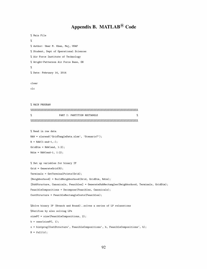
Appendix B. MATLAB R© Code% Main File
%
% Author: Umar M. Khan, Maj, USAF
% Student, Dept of Operational Sciences
% Air Force Institute of Technology
% Wright-Patterson Air Force Base, OH
%
% Date: February 14, 2014
clear
clc
% MAIN PROGRAM
%%%%%%%%%%%%%%%%%%%%%%%%%%%%%%%%%%%%%%%%%%%%%%%%%%%%%%%%%%%%%%%%%%%%%%%%%%%
% PART I: PARTITION RECTANGLE %
%%%%%%%%%%%%%%%%%%%%%%%%%%%%%%%%%%%%%%%%%%%%%%%%%%%%%%%%%%%%%%%%%%%%%%%%%%%
% Read in raw data
RAW = xlsread(’GridTangleData.xlsm’, ’Scenario7’);
R = RAW(1:end-1,:);
GridDim = RAW(end, 1:2);
Rdim = RAW(end-1, 1:2);
% Set up variables for binary IP
Grid = GenerateGrid(R);
Terminals = GetTerminalPoints(Grid);
[Neighborhood] = BuildNeighborhood(Grid, GridDim, Rdim);
[SubStructure, Canonicals, Feasibles] = GenerateSubRectangles(Neighborhood, Terminals, GridDim);
FeasibleCompositions = Decompose(Feasibles, Canonicals);
CostStructure = FeasibleRectangleCosts(Feasibles);
%Solve binary IP (Branch and Bound)..solves a series of LP relaxations
%Verifies by also solving LPs
sizeFC = size(FeasibleCompositions, 2);
b = ones(sizeFC, 1);
x = bintprog(CostStructure’, FeasibleCompositions’, b, FeasibleCompositions’, b);
B = full(x);
92

Partition = IdentifyPartition(B, Feasibles);
VisualData = GenerateFigure(Terminals, Partition, Rdim);
%%%%%%%%%%%%%%%%%%%%%%%%%%%%%%%%%%%%%%%%%%%%%%%%%%%%%%%%%%%%%%%%%%%%%%%%%%%
% PART II: ASSIGN UAVs %
%%%%%%%%%%%%%%%%%%%%%%%%%%%%%%%%%%%%%%%%%%%%%%%%%%%%%%%%%%%%%%%%%%%%%%%%%%%
MISSION_DURATION = 48; % hours of surveillance - modify as needed
MAX_REVISIT_TIME = 9; % DM’s desired maximum revisit time in hours
U = InitializeUAVs();
Mapping = Match(U, Partition, MISSION_DURATION, MAX_REVISIT_TIME);
Q = PrintMapping(Partition, Mapping);
%-----------------------------------------------------------------------
% CLASSES
classdef GridPoint
%GridPoint objects are: Terminal, Steiner, and edge points of R
% Ref: Meneses and Souza (1998); point objects are used to define
% objects of class FeasibleRectangle
properties
x
y
type
nXpos = Neighbor;
nYpos = Neighbor;
nXneg = Neighbor;
nYneg = Neighbor;
end
methods
% class constructor
function p = GridPoint(c1, c2, t)
p.x = c1;
p.y = c2;
p.type = t;
end
93
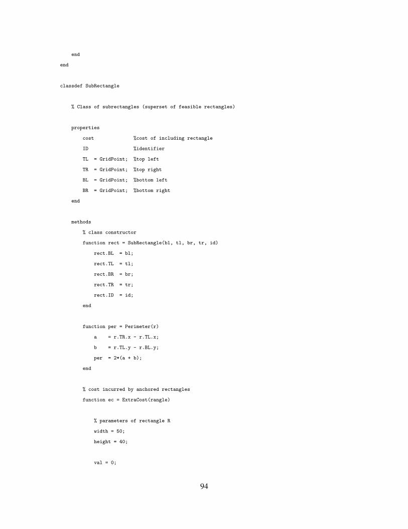
end
end
classdef SubRectangle
% Class of subrectangles (superset of feasible rectangles)
properties
cost %cost of including rectangle
ID %identifier
TL = GridPoint; %top left
TR = GridPoint; %top right
BL = GridPoint; %bottom left
BR = GridPoint; %bottom right
end
methods
% class constructor
function rect = SubRectangle(bl, tl, br, tr, id)
rect.BL = bl;
rect.TL = tl;
rect.BR = br;
rect.TR = tr;
rect.ID = id;
end
function per = Perimeter(r)
a = r.TR.x - r.TL.x;
b = r.TL.y - r.BL.y;
per = 2*(a + b);
end
% cost incurred by anchored rectangles
function ec = ExtraCost(rangle)
% parameters of rectangle R
width = 50;
height = 40;
val = 0;
94
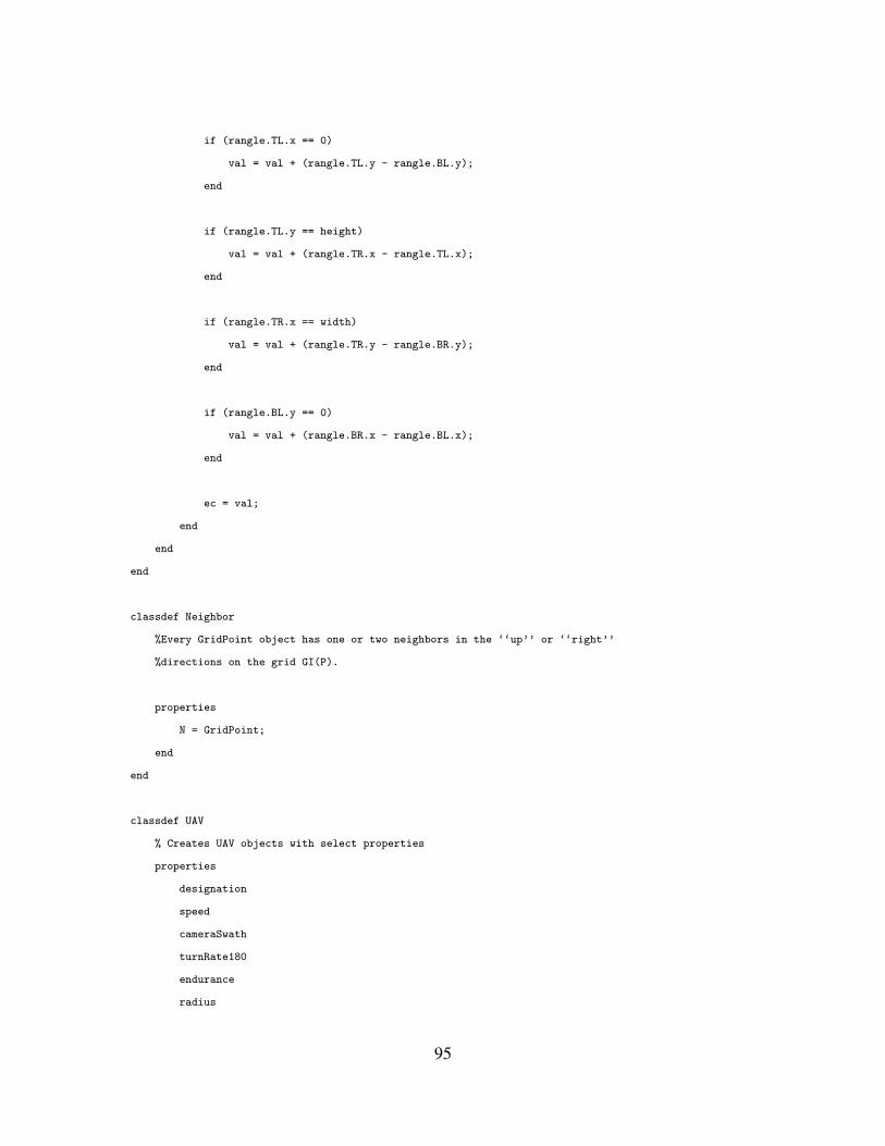
if (rangle.TL.x == 0)
val = val + (rangle.TL.y - rangle.BL.y);
end
if (rangle.TL.y == height)
val = val + (rangle.TR.x - rangle.TL.x);
end
if (rangle.TR.x == width)
val = val + (rangle.TR.y - rangle.BR.y);
end
if (rangle.BL.y == 0)
val = val + (rangle.BR.x - rangle.BL.x);
end
ec = val;
end
end
end
classdef Neighbor
%Every GridPoint object has one or two neighbors in the ‘‘up’’ or ‘‘right’’
%directions on the grid GI(P).
properties
N = GridPoint;
end
end
classdef UAV
% Creates UAV objects with select properties
properties
designation
speed
cameraSwath
turnRate180
endurance
radius
95

end
methods
% class constructor
function u = UAV(d, s, cs, tr, e, r)
u.designation = d;
u.speed = s;
u.cameraSwath = cs;
u.turnRate180 = tr;
u.endurance = e;
u.radius = r;
end
end
end
classdef Assignment
% Objects include subrectangles and their assigned UAV types
% along with how many of each UAV is required for the mission
% duration.
properties
rect = SubRectangle;
vehicle = UAV;
count % number of the assigned UAV needed
revisitTime
end
methods
% class constructor
function A = Assignment(SubRect, AirVehicle, num, rt)
A.rect = SubRect;
A.vehicle = AirVehicle;
A.count = num;
A.revisitTime = rt;
end
end
end
%-----------------------------------------------------------------------
% FUNCTIONS
96

function [P] = IdentifyPartition(B, F)
% Use output of bintprog to identify feasible rectangles
% in optimal partition (lowest cost).
sizeB = size(B,1);
part = SubRectangle.empty;
k = 1;
for m = 1:sizeB
if (B(m) == 1)
% Collect partition elements
part(k) = F(m);
k = k+1;
end
end
[P] = part;
end
function [PlotValues] = GenerateFigure(T, P, plotDims)
% Draw a plot of terminals
numTerminals = size(T, 2);
terminalList = zeros(numTerminals, 2);
xMax = plotDims(1);
yMax = plotDims(2);
k = 1;
for m = 1:numTerminals
terminalList(k, 1) = T(m).x;
terminalList(k, 2) = T(m).y;
k = k + 1;
end
sizeP = size(P,2);
figure(1)
97

plot(terminalList(:,1), terminalList(:,2), ’r*’)
axis([0 xMax 0 yMax])
figure(2)
plot(terminalList(:,1), terminalList(:,2), ’r*’)
axis([0 xMax 0 yMax])
hold on
for n = 1:sizeP
plot([P(n).TL.x, P(n).TR.x], [P(n).TL.y, P(n).TR.y])
plot([P(n).TL.x, P(n).BL.x], [P(n).TL.y, P(n).BL.y])
plot([P(n).BL.x, P(n).BR.x], [P(n).BL.y, P(n).BR.y])
plot([P(n).TR.x, P(n).BR.x], [P(n).TR.y, P(n).BR.y])
end
[PlotValues] = terminalList;
end
function [A] = GenerateGrid(rawData)
% Pass a list of ordered pairs.
% Output an array of GridPoint objects (a ‘‘rectangle’’).
rows = size(rawData,1);
GridPoints = GridPoint.empty;
for m = 1:rows
GridPoints(m) = GridPoint(rawData(m,1),rawData(m,2),rawData(m,3));
end
[A] = GridPoints;
end
function [T] = GetTerminalPoints(GT)
% Get list of terminal points
sizeGT = size(GT,2);
Terminals = GridPoint.empty;
k = 1;
for m = 1:sizeGT
98

if (GT(m).type == 1)
Terminals(k) = GT(m);
k = k+1;
end
end
[T] = Terminals;
end
function [N] = BuildNeighborhood(GT, GD, RD)
% For a given array of GridPoint objects - a ‘‘GridTangle’’ (GT),
% produce the neighbors - up, right, down, left - of each point.
sizeGT = size(GT,2);
% parameters specific to each rectangle R
xDimMax = GD(1);
width = RD(1);
height = RD(2);
% up and right neighbors
for k = 1:sizeGT
if (GT(k).y == height) && (k < sizeGT)
GT(k).nXpos = GT(k+1);
%GT(k).nYpos is null
elseif (GT(k).x == width) && (k <= sizeGT-xDimMax)
%GT(k).nXpos is null
GT(k).nYpos = GT(k+xDimMax);
elseif (GT(k).x == width) && (GT(k).y == height)
%do nothing
else
GT(k).nXpos = GT(k + 1);
GT(k).nYpos = GT(k + xDimMax);
end
end
% down and left neighbors
for z = sizeGT:-1:1
if (GT(z).y == 0) && (z > 1)
GT(z).nXneg = GT(z-1);
99

%GT(z).nYneg is null
elseif (GT(z).x == 0) && (z > 1)
%GT(z).nXneg is null
GT(z).nYneg = GT(z-xDimMax);
elseif (GT(z).x == 0) && (GT(z).y == 0)
%do nothing
else
GT(z).nXneg = GT(z - 1);
GT(z).nYneg = GT(z - xDimMax);
end
end
[N] = GT;
end
function [S, C, F] = GenerateSubRectangles(N, T, GD)
% Input some ‘‘GridTangle’’ (N) and output the set of all subrectangles.
% Output includes infeasible rectangles.
SR = SubRectangle.empty;
Canonicals = SubRectangle.empty;
Feasibles = SubRectangle.empty;
% parameters - modify for each input rectangle R
xDimMax = GD(1);
yDimMax = GD(2);
chunkSize = yDimMax - 1;
neighborhoodSize = size(N,2);
numTerminals = size(T,2);
id = 1;
cid = 1;
fid = 1;
% HORIZONTAL SUBRECTANGLE GENERATION
for t = 1:chunkSize
maxIndex = neighborhoodSize - t*xDimMax - 1;
100
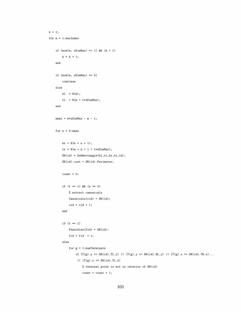
k = 1;
for m = 1:maxIndex
if (mod(m, xDimMax) == 1) && (m > 1)
k = k + 1;
end
if (mod(m, xDimMax) == 0)
continue
else
bl = N(m);
tl = N(m + t*xDimMax);
end
nmax = k*xDimMax - m - 1;
for n = 0:nmax
br = N(m + n + 1);
tr = N(m + n + 1 + t*xDimMax);
SR(id) = SubRectangle(bl,tl,br,tr,id);
SR(id).cost = SR(id).Perimeter;
count = 0;
if (t == 1) && (n == 0)
% extract canonicals
Canonicals(cid) = SR(id);
cid = cid + 1;
end
if (t == 1)
Feasibles(fid) = SR(id);
fid = fid + 1;
else
for g = 1:numTerminals
if (T(g).y >= SR(id).TL.y) || (T(g).y <= SR(id).BL.y) || (T(g).x >= SR(id).TR.x)...
|| (T(g).x <= SR(id).TL.x)
% terminal point is not in interior of SR(id)
count = count + 1;
101

end
end
if (count == numTerminals)
Feasibles(fid) = SR(id);
fid = fid + 1;
end
end
id = id + 1;
end
end
end
[S] = SR;
[C] = Canonicals;
[F] = Feasibles;
end
function [FC] = Decompose(F, C)
% take feasible rectangles and associate canonicals
% a_ij = 0 if feasible rectangle j contains canonical i
sizeF = size(F,2);
sizeC = size(C,2);
FeasibleCompositions = zeros(sizeF, sizeC);
for m = 1:sizeF
for n = 1:sizeC
if (C(n).BL.x >= F(m).BL.x) && (C(n).BR.x <= F(m).BR.x) && (C(n).BL.y >= F(m).BL.y)...
&& (C(n).TL.y <= F(m).TL.y)
FeasibleCompositions(m,n) = 1;
end
end
end
[FC] = FeasibleCompositions;
end
102
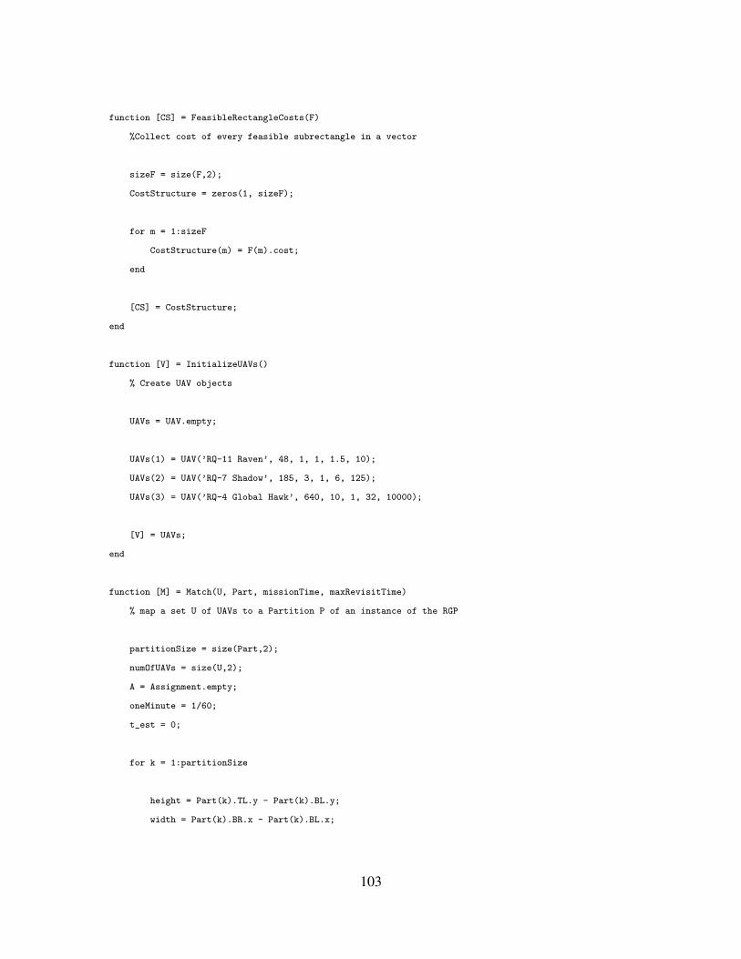
function [CS] = FeasibleRectangleCosts(F)
%Collect cost of every feasible subrectangle in a vector
sizeF = size(F,2);
CostStructure = zeros(1, sizeF);
for m = 1:sizeF
CostStructure(m) = F(m).cost;
end
[CS] = CostStructure;
end
function [V] = InitializeUAVs()
% Create UAV objects
UAVs = UAV.empty;
UAVs(1) = UAV(’RQ-11 Raven’, 48, 1, 1, 1.5, 10);
UAVs(2) = UAV(’RQ-7 Shadow’, 185, 3, 1, 6, 125);
UAVs(3) = UAV(’RQ-4 Global Hawk’, 640, 10, 1, 32, 10000);
[V] = UAVs;
end
function [M] = Match(U, Part, missionTime, maxRevisitTime)
% map a set U of UAVs to a Partition P of an instance of the RGP
partitionSize = size(Part,2);
numOfUAVs = size(U,2);
A = Assignment.empty;
oneMinute = 1/60;
t_est = 0;
for k = 1:partitionSize
height = Part(k).TL.y - Part(k).BL.y;
width = Part(k).BR.x - Part(k).BL.x;
103

if width >= height
for r = 1:numOfUAVs
x = 0;
if height <= U(r).cameraSwath
t_est = oneMinute + 2*width/U(r).speed;
else
t_est = (2*width*height/U(r).cameraSwath)/U(r).speed ...
+ oneMinute*(2*height/U(r).cameraSwath - 1);
end
if t_est <= maxRevisitTime
numUAVs = ceil(missionTime/U(r).endurance);
A(k) = Assignment(Part(k), U(r), round(numUAVs), t_est);
x = x + 1;
break
end
end
if x == 0 % no UAV meets revisit time criterion
A(k) = Assignment(Part(k), UAV(’None’, 0,0,0,0,0), 0, t_est);
end
else % height > width
for n = 1:numOfUAVs
x = 0;
if width <= U(n).cameraSwath
t_est = oneMinute + 2*height/U(n).speed;
else
t_est = (2*width*height/U(n).cameraSwath)/U(n).speed ...
+ oneMinute*(2*width/U(n).cameraSwath - 1);
end
if t_est <= maxRevisitTime
104
numUAVs = ceil(missionTime/U(n).endurance);
A(k) = Assignment(Part(k), U(n), round(numUAVs), t_est);
x = x + 1;
break
end
end
if x == 0
A(k) = Assignment(Part(k), UAV(’None’, 0,0,0,0,0), 0, t_est);
end
end
end
[M] = A;
end
function [V] = PrintMapping(P, M)
% Print Mapping Solution
sizeP = size(P,2);
for m = 1:sizeP
[P(m).TL.x P(m).TL.y P(m).BR.x P(m).BR.y]
width = P(m).TR.x - P(m).TL.x;
height = P(m).TL.y - P(m).BL.y;
[width, height]
M(m).vehicle.designation
M(m).count
M(m).revisitTime
end
[V] = 1;
end
105

Bibliography
[1] “C-17 Globemaster III Factsheet”, 2008. URL http://www.172aw.ang.af.mil/
resources/factsheets/factsheet.asp?fsID=12699&page=2.
[2] “Platforms for Persistent Communications, Surveillance and Reconnaissance”. ArmyScience Board Report, 2008.
[3] “FY2009-2034 Unmanned Systems Integrated Roadmap”. U.S. Department of De-fense, 2010.
[4] “Global Hawk unloading from C-5 Galaxy”, 2011. URL http://www.goodfellow.
af.mil/news/story.asp?id=123272577.
[5] “Agencies Could Improve Information Sharing and End-Use Monitoring on Un-manned Aerial Vehicle Exports”. GAO Report, 2012.
[6] “Gallery of USAF Weapons”. Air Force Magazine, 2012.
[7] “JP 2-01: Joint and National Intelligence Support to Military Operations”. U.S. De-partment of Defense, 2012.
[8] “Department of Defense Dictionary of Military and Associated Terms”. U.S. Depart-ment of Defense Report, 2013.
[9] “JP 2-0: Joint Intelligence”. Joint Military Doctrine, 2013.
[10] “UN Starts Drone Surveillance in DR Congo”, 2013. URL http://www.bbc.com/
news/world-africa-25197754.
[11] “MATLAB R© documentation”, 2014. URL http://www.mathworks.com/help/
optim/ug/binary-integer-programming-algorithms.html.
[12] “MQ-8 Fire Scout”, 2014. URL http://www.navair.navy.mil/index.cfm?
fuseaction=home.display&key=8250AFBA-DF2B-4999-9EF3-0B0E46144D03.
[13] “RQ-4A/B Global Hawk HALE Reconnaissance UAV, United States of Amer-ica”, 2014. URL http://www.airforce-technology.com/projects/
rq4-global-hawk-uav/.
[14] Ahmadzadeh, Ali, Gilad Buchman, Peng Cheng, Ali Jadbabaie, Jim Keller, VijayKumar, and George Pappas. “Cooperative control of UAVs for Search and Coverage”.Proceedings of the AUVSI Conference on Unmanned Systems. Orlando, FL. August29–31, 2006.
[15] Ahmadzadeh, Ali, James Keller, Ali Jadbabaie, and Vijay Kumar. “Multi-UAV Co-operative Surveillance with Spatio-Temporal Specifications”. 45th IEEE Conferenceon Decision and Control. San Diego, CA. December 13–15, 2006.
106

[16] Akella, Mohan, Sharad Gupta, and Avijit Sarkar. “Branch and Price: Column Genera-tion for Solving Huge Integer Programs”, 2014. URL http://www.acsu.buffalo.
edu/~nagi/courses/684/price.pdf.
[17] Barr, Alistair. “Amazon testing delivery by drone, CEO Bezos says”. USAToday, 2013. URL http://www.usatoday.com/story/tech/2013/12/01/
amazon-bezos-drone-delivery/3799021/.
[18] Carlsson, John. “Dividing a Territory among Several Vehicles”, INFORMS Journalon Computing, 24:565–577, 2012.
[19] Cavas, Christopher. “Fire Scout UAVs bound for Afghanistan”, 2011.URL http://www.navytimes.com/article/20110421/NEWS/104210326/
Fire-Scout-UAVs-bound-Afghanistan.
[20] Chepoi, Victor, Karim Nouioua, and Yann Vaxes. “A Rounding Algorithm forApproximating Minimum Manhattan Networks”, Theoretical Computer Science,390(1):56–69, 2008.
[21] Choset, Howie. “Coverage for Robotics &Ndash; A Survey of Recent Results”, An-nals of Mathematics and Artificial Intelligence, 31(1-4):113–126, 2001.
[22] Choset, Howie and Philippe Pignon. “Coverage Path Planning: The BoustrophedonDecomposition”. 1st International Conference on Field and Service Robotics. Can-berra, Australia, 1997.
[23] Erwin, Sandra. “For U.S. Air Force, the Cost of Operating Unmanned AircraftBecoming Unsustainable”, 2011. URL http://www.nationaldefensemagazine.
org/blog/Lists/Posts/Post.aspx?ID=523.
[24] Garfinkel, Robert. “An Improved Algorithm for the Bottleneck Assignment Problem”,Operations Research, 19(7):1747–1751, 1971.
[25] Garfinkel, Robert and George Nemhauser. Integer Programming. Wiley, New York,1972.
[26] Gudmundsson, Joachim, Christos Levcopoulos, and Giri Narasimhan. “Approximat-ing a Minimum Manhattan Network”, Nordic J. Comput, 8:2001, 1999.
[27] Ha, Taegyun. The UAV Continuous Coverage Problem. Master’s thesis, Air ForceInstitute of Technology, 2010.
[28] Hert, Susan and Vladimir Lumelsky. “Polygon Area Decomposition for Multiple-Robot Workspace Division”, International Journal of Computational Geometry andApplications, 8:437–466, 1998.
107

[29] Huang, Wesley. “Optimal Line-sweep-based Decompositions for Coverage Algo-rithms”. Proceedings of the 2001 IEEE International Conference on Robotics andAutomation. Seoul, South Korea. May 21–26, 2001.
[30] Marwedel, Peter, Lothar Thiele, and Frank Vahid. “Partitioning Algorithms...” com-piled lecture notes, n.d.
[31] Maza, Ivan and Anibal Ollero. “Multiple UAV Cooperative Searching Operationusing Polygon Area Decomposition and Efficient Coverage Algorithms”. School ofEngineering, University of Seville, 2006.
[32] de Meneses, Cludio Nogueira and Cid Carvalho de Souza. “Exact Solutions of Rect-angular Partitions via Integer Programming”. Universidade Estadual de Campinas,Instituto de Computacao, Campinas/SP, Brazil, 1998.
[33] Nigam, Nikhil. Control and Design of Multiple Unmanned Air Vehicles for PersistentSurveillance. Ph.D. thesis, Stanford University, 2009.
[34] Nigam, Nikhil and Ilan Kroo. “Persistent Surveillance Using Multiple Unmanned AirVehicles”. Proceedings of the IEEE Aerospace Conference. Big Sky, MT. March 1–8,2008.
[35] O’Rourke, Joseph and Geetika Tewari. “The Structure of Optimal Partitions of Or-thogonal Polygons into Fat Rectangles”, Computational Geometry, 28:49–71, 2004.
[36] Ousingsawat, Jarurat. “UAV Path Planning for Maximum Coverage Surveillance ofArea with Different Priorities”. The 20th Conference of Mech. Engineering Networkof Thailand. Nakhon Ratchasima, Thailand. October 18–20, 2006.
[37] Pohl, Adam J. Multiobjective UAV Mission Planning using Evolutionary Computa-tion. Master’s thesis, Air Force Institute of Technology, 2008.
[38] Quijano, Humberto and Leonardo Garrido. “Improving Cooperative Robot Explo-ration Using an Hexagonal World Representation”. Electronics, Robotics and Au-tomotive Mechanics Conference. Cuernacava, Morelos, Mexico. September 25–28,2007.
[39] Rader, David. Deterministic Operations Research. Wiley, New Jersey, 2010.
[40] Stone, Andrea. “Drone Program Aims To Accelerate Use Of Unmanned Air-craft By Police”, 2012. URL http://www.huffingtonpost.com/2012/05/22/
drones-dhs-program-unmanned-aircraft-police_n_1537074.html.
[41] Yanmaz, Evsen. “Connectivity Versus Area Coverage in Unmanned Aerial VehicleNetworks”. IEEE International Conference on Communications. Ottawa, Canada.June 10–15, 2012.
108

REPORT DOCUMENTATION PAGE Form ApprovedOMB No. 0704–0188
The public reporting burden for this collection of information is estimated to average 1 hour per response, including the time for reviewing instructions, searching existing data sources, gathering andmaintaining the data needed, and completing and reviewing the collection of information. Send comments regarding this burden estimate or any other aspect of this collection of information, includingsuggestions for reducing this burden to Department of Defense, Washington Headquarters Services, Directorate for Information Operations and Reports (0704–0188), 1215 Jefferson Davis Highway,Suite 1204, Arlington, VA 22202–4302. Respondents should be aware that notwithstanding any other provision of law, no person shall be subject to any penalty for failing to comply with a collectionof information if it does not display a currently valid OMB control number. PLEASE DO NOT RETURN YOUR FORM TO THE ABOVE ADDRESS.
1. REPORT DATE (DD–MM–YYYY) 2. REPORT TYPE 3. DATES COVERED (From — To)
4. TITLE AND SUBTITLE 5a. CONTRACT NUMBER
5b. GRANT NUMBER
5c. PROGRAM ELEMENT NUMBER
5d. PROJECT NUMBER
5e. TASK NUMBER
5f. WORK UNIT NUMBER
6. AUTHOR(S)
7. PERFORMING ORGANIZATION NAME(S) AND ADDRESS(ES) 8. PERFORMING ORGANIZATION REPORTNUMBER
9. SPONSORING / MONITORING AGENCY NAME(S) AND ADDRESS(ES) 10. SPONSOR/MONITOR’S ACRONYM(S)
11. SPONSOR/MONITOR’S REPORTNUMBER(S)
12. DISTRIBUTION / AVAILABILITY STATEMENT
13. SUPPLEMENTARY NOTES
14. ABSTRACT
15. SUBJECT TERMS
16. SECURITY CLASSIFICATION OF:
a. REPORT b. ABSTRACT c. THIS PAGE
17. LIMITATION OFABSTRACT
18. NUMBEROFPAGES
19a. NAME OF RESPONSIBLE PERSON
19b. TELEPHONE NUMBER (include area code)
Standard Form 298 (Rev. 8–98)Prescribed by ANSI Std. Z39.18
27–03–2014 Master’s Thesis Aug 2012 – Mar 2014
OPTIMAL PARTITIONING OF A SURVEILLANCE SPACE FORPERSISTENT COVERAGE USING
MULTIPLE AUTONOMOUS UNMANNED AERIAL VEHICLES:AN INTEGER PROGRAMMING APPROACH
Khan, Umar M., Major, USAF
Air Force Institute of TechnologyGraduate School of Engineering and Management (AFIT/EN)2950 Hobson WayWPAFB OH 45433-7765
AFIT-ENS-14-M-16
Intentionally Left Blank
Distribution Statement A: Approved for Public Release; Distribution Unlimited
This material is declared a work of the U.S. Government and is not subject to copyright protection in the United States.
Unmanned aerial vehicles (UAVs) are an essential tool for the battlefield commander in part because theyrepresent an attractive intelligence gathering platform that can quickly identify targets and track movements ofindividuals within areas of interest. In order to provide meaningful intelligence in near-real time during a mission, itmakes sense to operate multiple UAVs with some measure of autonomy to survey the entire area persistently over themission timeline. This research considers a space where intelligence has identified a number of locations and theirsurroundings that need to be monitored for a period of time. An integer program is formulated and solved to partitionthis surveillance space into the minimum number of subregions such that these locations fall outside of each partitionedsubregion for efficient, persistent surveillance of the locations and their surroundings. Partitioning is followed by aUAV-to-partitioned subspace matching algorithm so that each subregion of the partitioned surveillance space is assignedexactly one UAV. Because the size of the partition is minimized, the number of UAVs used is also minimized.
Set Partitioning, Integer Programming, Persistent Surveillance, Unmanned Aerial Vehicles
U U U UU 121
James W. Chrissis, Ph.D., AFIT/ENS
(937) 255–3636 ext 4606; [email protected]


![Optimal Partitioning of Distribution Networks for Micro …file.scirp.org/pdf/JPEE_2017092614124380.pdf · rule-based approaches [6] [7], genetic algorithms[8], and mathematical pr](https://img.dokumen.tips/doc/110x75/5b59da617f8b9a31668da2d7/optimal-partitioning-of-distribution-networks-for-micro-filescirporgpdfjpee.jpg)
![Optimal Partitioning for Classification and …...ing optimal trees (i.e., trees having the minimal expected loss for their size) [37], [38], practical procedures for constructing](https://img.dokumen.tips/doc/110x75/5f41eeaf133b5e582e1ccdbb/optimal-partitioning-for-classification-and-ing-optimal-trees-ie-trees-having.jpg)