GEOSTATISTICAL INFERENCE UNDER · PDF filePeter J Diggle (Lancaster ... Geostatistics involves the fitting of spatially continuous models to spatially discrete data (Chilès and Delfiner,

Johns Hopkins University, Dept. of Biostatistics Working Papers

1-6-2008

GEOSTATISTICAL INFERENCE UNDERPREFERENTIAL SAMPLINGPeter J. DiggleLancaster University and the Johns Hopkins Bloomberg School of Public Health, [email protected]

Raquel MenezesUniversity of Minho

Ting-li SuLancaster University

This working paper is hosted by The Berkeley Electronic Press (bepress) and may not be commercially reproduced without the permission of thecopyright holder.Copyright © 2011 by the authors

Suggested CitationDiggle, Peter J.; Menezes, Raquel; and Su, Ting-li, "GEOSTATISTICAL INFERENCE UNDER PREFERENTIAL SAMPLING"( January 2008). Johns Hopkins University, Dept. of Biostatistics Working Papers. Working Paper 162.http://biostats.bepress.com/jhubiostat/paper162

http://biostats.bepress.com/jhubiostat

Geostatistical Inference Under Preferential Sampling

Peter J Diggle

(Lancaster University and Johns Hopkins University School of Public Health),Raquel Menezes

(University of Minho)and

Ting-li Su(Lancaster University)

January 6, 2008

Abstract

Geostatistics involves the fitting of spatially continuous models to spatially discrete data(Chiles and Delfiner, 1999). Preferential sampling arises when the process that determinesthe data-locations and the process being modelled are stochastically dependent. Conventionalgeostatistical methods assume, if only implicitly, that sampling is non-preferential. However,these methods are often used in situations where sampling is likely to be preferential. Forexample, in mineral exploration samples may be concentrated in areas thought likely to yieldhigh-grade ore. We give a general expression for the likelihood function of preferentially sam-pled geostatistical data and describe how this can be evaluated approximately using MonteCarlo methods. We present a model for preferential sampling, and demonstrate through simu-lated examples that ignoring preferential sampling can lead to seriously misleading inferences.We describe an application of the model to a set of bio-monitoring data from Galicia, northernSpain, in which making allowance for preferential sampling materially changes the inferences.

Key words: environmental monitoring; geostatistics; marked point processes; Monte Carloinference; preferential sampling; spatial statistics.

1

Hosted by The Berkeley Electronic Press

1 Introduction

The term geostatistics describes the branch of spatial statistics in which data are obtainedby sampling a spatially continuous phenomenon S(x) : x ∈ IR2 at a discrete set of locationsxi : i = 1, ..., n in a spatial region of interest A ⊂ IR2. In many cases, S(x) cannot be measuredwithout error. Measurement errors in geostatistical data are typically assumed to be additive,possibly on a transformed scale. Hence, if Yi denotes the measured value at the location xi, asimple model for the data takes the form

Yi = µ + S(xi) + Zi : i = 1, ..., n (1)

where the Zi are mutually independent, zero-mean random variables. We adopt the conventionthat E[S(x)] = 0 for all x, hence in (1) E[Yi] = µ for all i. The model (1) extends easily tothe regression setting, in which E[Yi] = µi = d′

iβ, with di a vector of explanatory variablesassociated with Yi. The objectives of a geostatistical analysis typically focus on prediction ofproperties of the realisation of S(x) throughout the region of interest A. Targets for predictionmight include, according to context: the value of S(x) at an unsampled location; the spatialaverage of S(x) over A or sub-sets thereof; the minimum or maximum value of S(x); orsub-regions in which S(x) exceeds a particular threshold. Chiles and Delfiner (1999) give acomprehensive account of classical geostatistical models and methods.

Diggle, Moyeed and Tawn (1998) introduced the term model-based geostatistics to mean theapplication of general principles of statistical modelling and inference to geostatistical prob-lems. In particular, they added Gaussian distributional assumptions to the classical model(1) and re-expressed it as a two-level hierarchical linear model, in which S(x) is the value atlocation x of a latent Gaussian stochastic process and, conditional on S(xi) : i = 1, ..., n, themeasured values Yi : i = 1, ..., n are mutually independent, Normally distributed with meansµ + S(xi) and common variance τ 2. Diggle, Moyeed and Tawn (1998) then extended thismodel, retaining the Gaussian assumption for S(x) but allowing a generalized linear model(McCullagh and Nelder, 1989) for the mutually independent conditional distributions of theYi given S(xi).

As a convenient shorthand notation to describe the hierarchical structure of a geostatisticalmodel, we use [·] to mean “the distribution of,” and write S = {S(x) : x ∈ IR2} and Y =(Y1, ..., Yn). Then, the Diggle, Moyeed and Tawn (1998) model has the simple structure[S, Y ] = [S][Y |S] = [S][Y1|S(x1)][Y2|S(x2)]...[Yn|S(xn)]. Furthermore, in (1) the [Yi|S(xi)] areunivariate Gaussian distributions with means S(xi) and common variance τ 2

As presented above, and in almost all of the geostatistical literature, models for the data treatthe sampling locations xi either as fixed by design or otherwise stochastically independentof the process S(x), and hence of Y . Admitting the possibility that the sampling designmay be stochastic, and writing X = (x1, ..., xn), the structure of the model then becomes[X, S, Y ] = [X][S][Y |S], from which it is clear that conditioning on X does not affect inferencesabout S or Y . We refer to this as non-preferential sampling of geostatistical data. Conversely,preferential sampling refers to any situation in which [X, S, Y ] 6= [X][S, Y ].

We contrast the term non-preferential with the term uniform, the latter meaning that, be-forehand, all locations in A are equally likely to be sampled. Examples of designs which are

2

http://biostats.bepress.com/jhubiostat/paper162

both uniform and non-preferential include completely random designs and regular lattice de-signs (strictly, in the latter case, if the lattice origin is chosen at random). An example of anon-uniform, non-preferential design would be one in which sample locations are an indepen-dent random sample from a prescribed non-uniform distribution on A. Preferential designscan arise either because sampling locations are deliberately concentrated in sub-regions of Awhere the underlying values of S(x) are thought likely to be larger (or smaller) than average,or more generally when X and Y are the joint outcome of a marked point process in whichthere is dependence between the points, X, and the marks, Y .

We emphasise at this point that our definition of preferential sampling is as a stochasticphenomenon. A sampling design that deliberately focuses on sub-regions where the mean ofS(x), as opposed to its realised value, is atypically high, is not preferential. However, in mostgeostatistical applications it is difficult to maintain a sharp distinction between deterministicor stochastic variation in S(x) because of the absence of independent replication of the processunder investigation.

Curriero, Hohn, Liebhold and Lele (2002) evaluated a class of non-ergodic estimators for thecovariance structure of geostatistical data, which had been proposed by Isaaks and Srivastava(1988) and Srivastava and Parker (1989) as a way of dealing with preferential sampling, butconcluded that the non-ergodic estimators “possess no clear advantage” over the traditionalestimators that we describe in Section 3.1 below. Schlather, Ribeiro and Diggle (2004) devel-oped two tests for preferential sampling, which treat a set of geostatistical data as a realisationof a marked point process. Their null hypothesis is that the data are a realisation of a random

field model. This model assumes that the sample locations X are a realisation of a pointprocess P on A, that the mark of a point at location x is the value at x of the realisationof a random field S on A, and that P and S are independent processes. This is thereforeequivalent to our notion of non-preferential samplng. Their test statistics are based on theidea that, under the null hypothesis that sampling is non-preferential, the low-order momentproperties of pairs of measured values Yi and Yj should not depend on the distance betweenthe corresponding sampling locations xi and xj , and each test is implemented by compar-ing the observed value of the chosen test statistics with values calculated from simulationsof a conventional geostatistical model fitted to the data on the assumption that sampling isnon-preferential. Guan and Afsharatous (2007) avoid the need for simulation and parame-teric model-fitting by dividing the observation into non-overlapping sub-regions that can beassumed to provide approximately independent replicates of the test statistics. In practice,this requires a large data-set; their application has a sample size n = 4358.

In this paper, we propose a class of stochastic models and associated methods of likelihood-based inference for preferentially sampled geostatistical data. In Section 2 we define ourmodel for preferential sampling. In Section 3 we use the model to illustrate the potential formisleading inferences when conventional geostatistical methods are applied to preferentiallysampled data. Section 4 discusses likelihood-based inference using Monte Carlo methods.Section 5 applies our model and methods to a set of biomonitoring data from Galicia, northernSpain in which the data derive from two surveys, one preferentially sampled the other not, ofthe same region. Section 6 is a concluding discussion.

3


2 A shared latent process model for preferential sam-

pling

Recall that S denotes an unobserved, spatially continuous process on a spatial region A, Xdenotes a point process on A and Y denotes a set of measured values, one at each point of X.The focus of scientific interest is on properties of S, as revealed by the data (X, Y ), ratherthan on the joint properties of S and X, but we wish to protect against spurious inferencesthat might arise because of stochastic dependence between S and X.

To clarify the distinction between preferential and non-preferential sampling, and the inferen-tial consequences of the former, we first examine a related situation considered by Rathbun(1996), in which S and X are stochastically dependent but measurements Y are taken only ata different, pre-specified set of locations, i.e. independently of X. Then, the joint distributionof S, X and Y takes the form

[S, X, Y ] = [S][X|S][Y |S]. (2)

It follows immediately on integrating (2) with respect to X that the joint distribution of Sand Y has the standard form, [S, Y ] = [S][Y |S]. Hence, for inference about S it is valid, ifpotentially inefficient, to ignore X, i.e. to use conventional geostatistical methods. Modelsanalogous to (2) have also been proposed in a longitudinal setting, where the analogues of Yand X are a time-sequence of repeated measurements at pre-specified times and a related time-to-event outcome, respectively. See, for example, Wulfsohn and Tsiatis (1997) or Henderson,Diggle and Dobson (2000).

In contrast, if Y is observed at the points of X, the appropriate factorisation is

[S, X, Y ] = [S][X|S][Y |X, S]. (3)

Even when the algebraic form of [Y |X, S] reduces to [Y |S], an important distinction between(3) and (2) is that in (3) there is a functional dependence between S and X which cannot beignored; typically, [Y |S, X] = [Y |S0], where S0 = S(X) denotes the values of S(x) at all pointsx ∈ X. The implicit specification of [S, Y ] resulting from (3) is therefore non-standard, andconventional geostatistical inferences which ignore the stochastic nature of X are potentiallymisleading. The longitudinal analogue of (2) arises when subjects in a longitudinal studyprovide measurements at time-points which are not pre-specified as part of the study design;see, for example, Lipsitz, Fitzmaurice, Ibrahim, Gelber and Lipshultz (2002), Lin, Scharfsteinand Rosenheck (2004) or Ryu, Sinha, Mallick, Lipsitz and Lipshultz (2007).

We now define a specific class of models through the following additional assumptions;

A1. S is a stationary Gaussian process with mean µ, variance σ2 and correlation functionρ(u; φ) = Corr{S(x), S(x′)} for any x and x′ a distance u apart;

A2. conditional on S, X is an inhomogeneous Poisson process with intensity

λ(x) = exp{α + βS(x)}; (4)

4


A3. conditional on S and X, Y is a set of mutually independent Gaussian variates withYi ∼ N(S(xi), τ

2).

It follows from A1 and A2 that, unconditionally, X is a log-Gaussian Cox process (Møller,Syversveen and Waagepetersen, 1998). If β = 0 in (4), then it follows from A1 and A3 that theunconditional distribution of Y is multivariate Gaussian with mean µ1 and variance matrixτ 2I + σ2R, where I is the identity matrix and R has elements rij = ρ(||xi − xj ||; φ).

3 Impact of preferential sampling on geostatistical

inference

We have conducted a simulation experiment in which we simulated data on A the unit squarefrom an underlying stationary Gaussian process which we then sampled, with additive Gaus-sian measurement error, either non-preferentially or preferentially according to each of thefollowing sampling designs. For the completely random sampling design, sample locations xi

were an independent random sample from the uniform distribution on A. For the preferen-

tial design, the xi were generated from the model defined by equation (4), with parameterβ = 2. For the clustered design, we used the same model, but with one realisation of S togenerate the data Y and a second, independent realisation of S to generate X, thereby givinga non-preferential design with the same marginal properties as the preferential design.

The model for the spatial process S was stationary Gaussian, with mean µ = 4, varianceσ2 = 1.5, and Matern correlation with scale parameter φ = 0.15 and shape parameter κ = 1.In each case, the data yi consisted of the realised value of S(xi) plus an independent Gaussianmeasurement error with mean zero and variance τ 2 = 0.25.

The three panels of Figure 1 show a realisation of each of the three sampling designs super-imposed on a single realisation of the process S. The preferential nature of the sampling inthe central panel of Figure 1 is clear.

3.1 Variogram estimation

The theoretical variogram of a stationary spatial process Y (x) is the function V (u) = Var{Y (x)−Y (x′)} where u denotes the distance between x and x′. Non-parametric estimates of V (u)are widely used in geostatistical work, both for exploratory data analysis and for diagnosticchecking.

Consider a set of data (xi, yi) : i = 1, ..., n, where xi denotes a location and yi a correspondingmeasured value. The empirical variogram ordinates are the quantities vij = (yi − yj)

2/2.Under non-preferential sampling, each vij is an unbiased estimator for V (uij), where uij isthe distance between xi and xj . A scatterplot of vij against uij or, more usefully, a smoothedversion of this scatterplot, can be used to suggest appropriate parametric models for thespatial covariance structure of the data. For more information on variogram estimation, seefor example Cressie (1985; 1991, Chapter 2), Chiles and Delfiner (1999) or Diggle and Ribeiro

5


0.0 0.2 0.4 0.6 0.8 1.0

0.0

0.2

0.4

0.6

0.8

1.0

0.0 0.2 0.4 0.6 0.8 1.0

0.0

0.2

0.4

0.6

0.8

1.0

0.0 0.2 0.4 0.6 0.8 1.0

0.0

0.2

0.4

0.6

0.8

1.0

Figure 1: Sample locations and underlying realisations of the signal process for the model usedin the simulation study. The left-hand panel shows the completely random sample, the centre-panel the preferential sample and the right-hand panel the clustered sample. In each case, thegrey-scale image represents the realisation of the signal process, S(x), used to generate theassociated measurement data. The model parameter values are µ = 4, σ2 = 1.5, φ = 0.15,κ = 1, τ 2 = 0.25, β = 2

(2007, Chapter 5).

The two panels of Figure 2 show simulation-based estimates of the point-wise bias and stan-dard deviation of smoothed empirical variograms, derived from 500 replicate simulations ofeach of our three sampling designs. With regard to bias, the results under both uniformand clustered non-preferential sampling designs are consistent with the unbiasedness of theempirical variogram ordinates; although smoothing the empirical variogram ordinates doesinduce some bias, this effect is negligible in the current setting. In contrast, under preferen-tial sampling the results show severe bias. With regard to efficiency, the right-hand panel ofFigure 2 illustrates that clustered sampling designs, whether preferential or not, are also lessefficient than uniform sampling. The bias induced by preferential sampling is qualitativelyunsurprising. The implicit estimand of the empirical variogram is the variance of Y (x)−Y (x′)conditional on both x and x′ belonging to X, which in general will differ from the unconditionalvariance; see, for example, Walder and Stoyan (1996) or Schlather (2001).

3.2 Spatial prediction

Suppose that our target for prediction is S(x0), the value of the process S at a generic locationx0, given sample data (xi, yi), i = 1, 2, ..., n. The widely used ordinary kriging predictorestimates the unconditional expectation of S(x0) by generalised least squares, but using plug-in estimates of the parameters that define the covariance structure of Y . Traditionally, theseplug-in estimates would be obtained by matching theoretical and empirical variograms in someway; we used maximum likelihood estimates under the assumed Gaussian model for Y .

Table 2 shows 95% coverage intervals for the resulting biases and mean square prediction

6


0.0 0.1 0.2 0.3 0.4 0.5 0.6 0.7

0.0

0.2

0.4

0.6

0.8

1.0

1.2

distance

bias

random

preferential

clustered

0.0 0.1 0.2 0.3 0.4 0.5 0.6 0.7

0.0

0.5

1.0

1.5

2.0

distance

stdd

ev

random

preferential

clustered

Figure 2: Bias and standard deviation of the sample variogram under random, preferentialand clustered sampling. See text for detailed description of the simulation model.

Table 1: Impact of sampling design on the bias and mean square error of the ordinary krigingpredictor S(x0), when x0 = (0.5, 0.5) and each sample consists of 100 locations on the unitsquare. Each entry in the table is a 95% coverage interval calculated empirically from 500independent simulations. See text for detailed description of the simulation model.

Sampling designCompletely random Preferential (β = 2) Clustered

bias (−0.081, 0.059) (1.290, 1.578) (−0.082, 0.186)mean square error (0.268, 0.354) (2.967, 3.729) (0.948, 1.300)

errors of the ordinary kriging predictor S(x0), where x0 = (0.5, 0.5), in each case evaluatedempirically over 500 replicate simulations.

The bias is large and positive under preferential sampling. This prediction bias is a directconsequence of the bias in the estimation of the model parameters, which in turn arises becausethe preferential sampling model leads to the over-sampling of locations corresponding to highvalues of the underlying process S. The correct predictive distribution for S is [S|Y, X] which,with known parameter values, takes a standard multivariate Gaussian form whether or notsampling is preferential. The two non-preferential sampling designs both lead to approximatelyunbiased prediction, as predicted by theory. The substantially larger mean square error forclustered sampling by comparison with completely random sampling reflects the inefficiencyof the latter, as already illustrated in the context of variogram estimation.

7


4 Monte Carlo maximum likelihood estimation

For the shared latent process model (3), the likelihood function for data X and Y can beexpressed as

L(θ) = [X, Y ] = ES [[X|S][Y |X, S]] , (5)

where the expectation is with respect to the unconditional distribution of S. Evaluation ofthe conditional distribution [X|S] strictly requires the realisation of S to be available at allx ∈ A. In practice, we approximate the spatially continuous realisation of S by the set ofvalues of S on a fine lattice to cover A, and replace the exact locations X by their closestlattice points. We then partition S into S = {S0, S1}, where S0 denotes the values of S ateach of n data-locations xi ∈ X, and S1 denotes the values of S at the remaining N − nlattice-points.

To evaluate L(θ) approximately, a naive strategy would be to replace the intractable expecta-tion on the right hand side of (5) by a sample average over simulations Sj. This strategy failswhen the measurement error variance τ 2 is zero, because unconditional simulations of S willthen be incompatible with the observed Y . It also fails in practice when the measurementerror is small relative to the variance of S, which is the case of most practical interest.

We therefore re-write the exact likelihood (5) as the integral

L(θ) =∫

[X|S][Y |X, S][S|Y ]

[S|Y ][S]dS. (6)

Now, write [S] = [S0][S1|S0] and replace the term [S|Y ] in the denominator of (6) by[S0|Y ][S1|S0, Y ] = [S0|Y ][S1|S0]. Note also that [Y |X, S] = [Y |S0]. Then, (6) becomes

L(θ) =∫

[X|S][Y |S0]

[S0|Y ][S0][S|Y ]dS

= ES|Y

[

[X|S][Y |S0]

[S0|Y ][S0]

]

(7)

and a Monte Carlo approximation is

LMC(θ) = m−1

m∑

j=1

[

[X|Sj][Y |S0j]

[S0j |Y ][S0j ]

]

, (8)

where now the Sj are simulations of S conditional on Y . Note that when Y is measuredwithout error, [Y |S0j ]/[S0j|Y ] = 1. To reduce the Monte Carlo variance, we also use anti-thetic pairs of realisations, i.e. for each j = 1, ..., m/2 set S2j = 2µc −S2j−1, where µc denotesthe conditional mean of S given Y .

To simulate a realisation from [S|Y ], we use the following construction. Recall that the data-locations X = {x1, ..., xn} constitute a sub-set of the N ≥ n prediction locations, X∗ ={x∗

1, ..., x∗

N} say. Define A to be the n by N matrix whose ith row consists of N − 1 zeros anda single 1 to identify the position of xi within X∗. Note that, unconditionally, S ∼ MVN(0, Σ)

8


and Y ∼ MVN(µ, Σ0) with Σ0 = AΣA′ + τ 2I. Then, if Z denotes an independent randomsample of size n from N(0, τ 2) and y denotes the observed value of Y , it follows that

Sc = S + ΣA′Σ−1

0(y − µ + Z − AS) (9)

has the required multivariate Gaussian distribution of S given Y = y (Rue and Held, 2005,Chapter 2; Eidsvik, Martino and Rue, 2006). Hence, for conditional simulation when N islarge, we need a fast algorithm for unconditional simulation of S, for which we use the circulantembedding algorithm of Wood and Chan (1994) applied to a rectangular region containingthe region of interest, A. The subsequent calculations for Sc then involve only the relativelystraightforward inversion of the n×n matrix Σ0 and simulation of the n independent Gaussianrandom variables that make up the vector Z in (9).

5 Heavy-metal bio-monitoring in Galicia

Our application concerns bio-monitoring of lead pollution in Galicia, northern Spain. The dataconsist of two spatial surveys of lead concentrations in moss samples, taken in 1997 and 2000.In the first survey, the sampling design was highly non-uniform and potentially preferential,whereas the second survey used a regular lattice design which is therefore non-preferential.For further details, see Fernandez, Rey and Carballeira (2000) and Aboal, Real, Fernandezand Carballeira (2005). One objective of analysing these data is to estimate, and compare,maps of lead concentrations in 1997 and 2000. Figure 3 shows the sampling locations for thetwo surveys.

Table 2: Summary statistics for lead pollution levels measured in 1997 and 2000.

untransformed log-transformed1997 2000 1997 2000

Number of locations 63 132 63 132Mean 4.72 2.15 1.44 0.66Standard deviation 2.21 1.18 0.48 0.43Minimum 1.67 0.80 0.52 -0.22Maximum 9.51 8.70 2.25 2.16

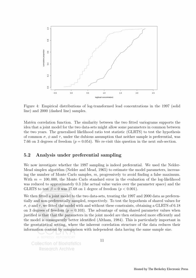
The measured lead concentrations included two gross outliers in 2000, each of which wereplaced by the average of the remaining values from that year’s survey. Table 2 gives summarystatistics for the resulting 1997 and 2000 data. Note that the mean response is higher forthe 1997 data than for the 2000 data, which would be consistent either with the formerbeing preferentially sampled near potential pollutant sources, or with an overall reduction inpollution levels over the three years between the two surveys. Also, the log-transformationeliminates an apparent variance-mean relationship in the data and leads to more symmetricdistributions of measured values (Figure 4).

9


5.0 5.5 6.0 6.5

46.5

47.0

47.5

48.0

48.5

19972000

Figure 3: Sampling locations for 1997 (solid dots) and 2000 (open circles). The unit of distanceis 100km.

5.1 Standard geostatistical analysis

For an initial analysis, we assume a standard linear Gaussian model for the underlying signalS(x), with mean µ, variance σ2, Matern correlation function ρ(u; φ, κ) and measurement errorvariance τ 2, and fit this model separately to the 1997 and 2000 data. The Matern (1986) classof correlation functions takes the form

ρ(u; φ, κ) = {2κ−1Γ(κ)}−1(u/φ)κKκ(u/φ) : u > 0,

where Kκ(·) denotes the modified Bessel function of the second kind, of order κ > 0. Thisclass is widely used because of its flexibility. Although κ is difficult to estimate withoutextensive data, the integral part of κ determines the degree of mean square differentiabilityof the corresponding process S(·), giving both a nice interpretation and, in at least somecontexts, a rationale for choosing a particular value for κ. The special case κ = 0.5 gives anexponential correlation function, ρ(u; φ) = exp(−u/φ).

Figure 5 shows, for each of 1997 and 2000, smoothed empirical variograms and theoreticalvariograms with parameters fitted by maximum likelihood. Based on the general shape ofthe two empirical variograms, we used a fixed value κ = 0.5 for the shape parameter of the

10


−0.5 0.0 0.5 1.0 1.5 2.0 2.5

0.0

0.2

0.4

0.6

0.8

1.0

log(lead concentration)

cum

ulat

ive

prop

ortio

n

Figure 4: Empirical distributions of log-transformed lead concentrations in the 1997 (solidline) and 2000 (dashed line) samples.

Matern correlation function. The similarity between the two fitted variograms supports theidea that a joint model for the two data-sets might allow some parameters in common betweenthe two years. The generalised likelihood ratio test statistic (GLRTS) to test the hypothesisof common σ, φ and τ , under the dubious assumption that neither sample is preferential, was7.66 on 3 degrees of freedom (p = 0.054). We re-visit this question in the next sub-section.

5.2 Analysis under preferential sampling

We now investigate whether the 1997 sampling is indeed preferential. We used the Nelder-Mead simplex algorithm (Nelder and Mead, 1965) to estimate the model parameters, increas-ing the number of Monte Carlo samples, m, progressively to avoid finding a false maximum.With m = 100, 000, the Monte Carlo standard error in the evaluation of the log-likelihoodwas reduced to approximately 0.3 (the actual value varies over the parameter space) and theGLRTS to test β = 0 was 27.68 on 1 degree of freedom (p < 0.001).

We then fitted a joint model to the two data-sets, treating the 1997 and 2000 data as preferen-tially and non-preferentially sampled, respectively. To test the hypothesis of shared values forσ, φ and τ , we fitted the model with and without these constraints, obtaining a GLRTS of 6.18on 3 degrees of freedom (p = 0.103). The advantage of using shared parameter values whenjustified is that that the parameters in the joint model are then estimated more efficiently andthe model is consequently better identified (Altham, 1984). This is particularly important inthe geostatistical setting, where the inherent correlation structure of the data reduces theirinformation content by comparison with independent data having the same sample size.

11


0.0 0.2 0.4 0.6 0.8 1.0 1.2

0.00

0.05

0.10

0.15

0.20

0.25

distance

sem

ivar

ianc

e

0.0 0.2 0.4 0.6 0.8 1.0 1.2

0.00

0.05

0.10

0.15

0.20

0.25

distancese

miv

aria

nce

Figure 5: Smoothed empirical (open circles) and fitted theoretical (lines) variograms for 1997(left-hand panel) and 2000 (right-hand panel) log-transformed lead concentration data.

Table 5.2 shows the Monte Carlo maximum likelihood estimates together with estimatedstandard errors and correlations for the model with shared σ, φ and τ . Standard errors andcorrelations were evaluated by fitting a quadratic surface to Monte Carlo log-likelihoods byordinary least squares. Parameter combinations were initially set as a 36 factorial designcentred on the Monte Carlo maximum likelihood estimates, with parameter values chosensubjectively after examining the trajectories through the parameter space taken by the variousruns of the Nelder-Mead optimisation algorithm. The quadratic surface was then re-fitted afteraugmenting this design with a 26 factorial on a more closely spaced set of parameter values,to check the stability of the results. Each evaluation of the log-likelihood used m = 10, 000conditional simulations. The non-negative parameters σ, φ and τ are estimated on a log-transformed scale, to improve the quadratic approximation to the log-likelihood surface.

Note that the expectation of S(·) shows a substantial fall between 1997 and 2000, and thatthe preferential sampling parameter estimate is negative, β = −1.007. The latter finding iscritically dependent on our allowing the two mean parameters to differ. Otherwise, becausethe observed average pollution level is substantially higher in 1997 than in 2000, we wouldhave been forced to conclude that the 1997 sampling was preferential with a positive value ofβ. One piece of evidence against this alternative interpretation is that, within the 1997 data,the observed pollution levels are lower in the over-sampled northern half of the region than inthe under-sampled southern half, consistent with a negative value of β.

What impact does the acknowledgement of preferential sampling make on the predicted 1997

12


Table 3: Monte Carlo maximum likelihood estimates of parameters in the joint model for the1997 and 2000 Galicia biomonitoring data. Approximate standard errors and correlations arecomputed from a quadratic fit to the Monte Carlo log-likelihood surface (see text for details)

Parameter Estimate Standard error Correlation matrixµ97 1.685 0.193 1.000 0.248 0.301 0.563 0.134 -0.017µ00 0.735 0.095 0.248 1.000 0.097 0.255 0.107 -0.124log(σ) -0.936 0.044 0.301 0.097 1.000 0.181 -0.547 0.088log(φ) -1.402 0.065 0.563 0.255 0.181 1.000 0.470 -0.188log(τ) -1.478 0.040 0.134 0.107 -0.547 0.470 1.000 -0.230β -1.007 0.212 -0.017 -0.124 0.088 -0.188 -0.230 1.000

pollution surface? Figure 6 shows the predicted surfaces T (x) = E[T (x)|X, Y ], where T (x) =exp{S(x)} denotes lead concentration on the untransformed scale, together with the pointwisedifferences between the two. Each surface is a Monte Carlo estimate based on m = 10, 000simulations, resulting in Monte Carlo standard errors of 0.026 or less. The predictions basedon the preferential sampling model have substantially wider range than those that assume non-preferential sampling (0.836 to 8.358 and 1.273 to 5.989, respectively). The difference surfacealso covers a relatively large range (−0.756 to 4.221) and shows strong spatial structure.Acknowledgement of the preferential sampling therefore has made a material difference to theprediction of the 1997 pollution surface.

6 Discussion

In this paper, we have shown that conventional geostatistical models and associated statisticalmethods can lead to very misleading inferences if the underlying data have been preferentiallysampled. We have proposed a simple model to take account of preferential sampling anddeveloped associated Monte Carlo methods to enable maximum likelihood estimation andlikelihood ratio testing within the proposed class of models. The resulting methods are com-putationally intensive, but comfortably within the capacity of a modern lap-top PC; all of thecomputations reported in the paper were run in this mode, using the R software environmentand associated CRAN packages. The data and R code are available from the first author onrequest.

The computation of the Monte Carlo likelihood uses direct simulation, as in Diggle and Grat-ton (1984), rather than Markov chain Monte Carlo. Hence, issues of convergence do not arise,and the variablity between replicate simulations gives a direct estimate of the size of the MonteCarlo error.

We have described an application to a set of environmental bio-monitoring data from Gali-cia, northern Spain. An important feature of these data is that they are derived from twospatial surveys of the region of interest, only one of which involved preferential sampling.

13


5.0 5.5 6.0 6.5

46.5

47.0

47.5

48.0

5.0 5.5 6.0 6.5

46.5

47.0

47.5

48.0

5.0 5.5 6.0 6.5

46.5

47.0

47.5

48.0

Figure 6: Predicted surface of lead concentrations in 1997 under preferential (left-hand panel)and non-preferential (centre panel) assumptions, together with the pointwise difference be-tween the two (right-hand panel). All three surfaces are plotted on a common scale, from−0.756 (red) to 8.358 (white)

This, coupled with our finding that several of the model parameters can be assumed to take acommon value for the two samples, led to a better identifed joint model for the two surveys.To illustrate this point, we also fitted the preferential sampling model to the 1997 data alone.Although, as reported earlier, the value of the maximised log-likelihood was obtained rela-tively easily, the subsequent quadratic fitting method to estimate the standard errors of themaximum likelihood estimates proved problematic. Using a 35 +25 factorial design analogousto the earlier 36 + 26 design for the model fitted to the 1997 and 2000 data jointly, and with10,000 simulations for each log-likelihood evaluation as before, the quadratic fit explainedonly 72% of the variation in the Monte Carlo log-likelihoods, compared with 93% for the jointmodel, the implied estimate of ∂2L/∂β2 was not significantly different from zero, and the ratioof largest to smallest eigenvalues of the Hessian matrix was 34.5, compared with 22.3 for thejoint model.

Alternative strategies for dealing with poorly identified model parameters could include treat-ing the preferential sampling parameter β as a sensitivity parameter, since its value is typicallynot of direct scientific interest, or using Bayesian methods with informative priors.

A natural response to a strongly non-uniform sampling design is to ask whether its spatialpattern could be explained by the pattern of spatial variation in a relevant covariate. Suppose,for the sake of illustration, that S is observed without error, that dependence between X and Sarises through their shared dependence on a latent variable, U , and that the joint distributionof X and S is of the form

[X, S] =∫

[X|U ][S|U ][U ]dU, (10)

so that X and S are conditionally independent given U . If the values of U were to be observed,we could then legitimately work with the conditional likelihood, [X, S|U ] = [X|U ][S|U ] andeliminate X by integration, exactly as is done implicitly when conventional geostatistical

14


methods are used. In practice, “observing” U means finding explanatory variables which areassociated both with X and with S, adjusting for their effects and checking that after thisadjustment there is little or no residual dependence between X and S. If so, the analysis couldthen proceed on the assumption that sampling is no longer preferential. Note, in this context,that any of the proposed tests for preferential sampling can be applied, albeit approximately,to residuals after fitting a regression model for the mean response.

References

Aboal, J.R., Real, C., Fernandez, J.A. and A. Carballeira (2006). Mapping the results ofextensive surveys: the case of atmospheric biomonitoring and terrestrial mosses. Science of

the Total Environment, 356, 256–274.

Altham, P.M.E. (1984). Improving the precision of estimation by fitting a model. Journal of

the Royal Statistical Society, B 46, 118–119.

Baddeley A, Møller J. and Waagepetersen R. (2000). Non- and semi-parametric estimationof interaction in inhomogeneous point patterns. Statistica Neerlandica 54, 329-350.

Chiles, J-P and Delfiner, P. (1999). Geostatistics. New York : Wiley.

Cox, D.R.(1972). The statistical analysis of dependencies in point processes. In Stochastic

Point Processes, ed P.A.W. Lewis, 55-66. New York : Wiley.

Cressie, N.A.C. (1985). Fitting variogram models by weighted least squares. Journal of the

International Association of Mathematical Geology, 17, 563–86.

Curriero, F.C., Hohn, M.E., Liebhold, A.M. and Lele, S.R. (2002). A statistical evaluation ofnon-ergodic variogram estimators. Environmental and Ecological Statistics, 9, 89–110.

Diggle, P.J. and Gratton, R.J. (1984). Monte Carlo methods of inference for implicit statisticalmodels (with Discussion). Journal of the Royal Statistical Society, B 46, 196–227.

Diggle, P.J., Moyeed, R.A. and Tawn, J.A. (1998). Model-based geostatistics (with Discus-sion). Applied Statistics 47 299–350.

Diggle, P.J. and Ribeiro, P.J. (2007). Model-based Geostatistics. New York: Springer.

Eidsvik, J., Martino, S. and Rue, H. (2006). Approximate Bayesian inference in spatial gen-eralized linear mixed models. Technical Report, STATISTICS 2/2006, Norwegian Universityof Science and Technology, Trondheim, Norway.

Fernandez, J.A., Rey, A. and Carballeira, A. (2000). An extended study of heavy metaldeposition in Galicia (NW Spain) based on moss analysis. Science of the Total Environment,254, 31–44.

Guan, Y. and Afshartous, D.R. (2007). Test for independence between marks and points ofmarked point processes: a subsamplng approach. Environmental and Ecological Statistics, 14,101–111.

15


Henderson, R., Diggle, P. and Dobson, A. (2000). Joint modelling of measurements and eventtime data. Biostatistics, 1, 465–480.

Isaaks, E.H. and Srivastava, R.M. (1988). Spatial continuity measures for probabilistic anddeterministic geostatistics. Mathematical Geology, 20, 313–341.

Lin, H, Scharfstein, D.O. and Rosenheck, R.A. (2004). Analysis of longitudinal data withirregular, outcome-dependent follow-up. Journal of the Royal Statistical Society, B 66, 791–813.

Lipsitz, S.R., Fitzmaurice, G.M., Ibrahim, J.G., Gelber, R. and Lipshultz, S. (2002). Param-eter estimation in longitudinal studies with outcome-dependent follow-up. Biometrics, 58,621–630. McCullagh, P. and Nelder, J.A. (1989). Generalized Linear Models (second edition).London : Chapman and Hall.

Matern, B. (1986). Spatial Variation (second edition). Berlin: Springer.

Møller, J., Syversveen, A. and Waagepetersen, R. (1998). Log Gaussian Cox processes. Scan-

dinavian Journal of Statistics, 25, 451–82.

Nelder, J.A. and Mead, R. (1965). A simplex method for function minimization. Computer

Journal, 7, 308–313.

Rathbun, S.L. (1996). Estimation of Poisson intensity using partially observed concomitantvariables. Biometrics, 52, 226–42.

Ripley, B.D. (1976). The second order analysis of stationary point processes. Journal of

Applied Probability 13, 255-266.

Ripley, B.D. (1977). Modelling spatial patterns (with discussion). Journal of the Royal

Statistical Society B 39, 172–212.

Rue, H. and Held, L. (2005). Gaussian Markov Random Fields: Theory and Applications.London: Chapman and Hall.

Ryu, D., Sinha, D., Mallick, B., Lipsitz, S.R. and Lipshultz, S.E. (2007). Longitudinal studieswith outcome-dependent follow-up: models and Bayesian regression. Journal of the American

Statistical Association, 102, 952–961.

Schlather, M. (2001). On the second-order characteristics of marked point processes. Bernoulli,7, 99–117.

Schlather, M., Ribeiro, P. J. and Diggle, P. J. (2004). Detecting dependence between marksand locations of marked point processes. Journal of the Royal Statistical Society, B 66, 79–93.

Srivastava, R.M., and Parker, H.M. (1989). Robust measures of spatial continuity. In Geo-

statistics, Volume 1, ed. M. Armstrong, 295–308. Boston: Kluwer.

Walder, O. and Stoyan, D. (1996). On variograms of point process statistics. Biometrical

Journal, 38, 895–905.

Wood, A. T. A. and Chan, G. (1994). Simulation of stationary Gaussian processes in [0, 1]d.Journal of Computational and Graphical Statistics, 3, 409–432.

16


Wulfsohn, M.S. and Tsiatis, A.A (1997). A joint model for survival and longitudinal datameasured with error. Biometrics, 53, 330–339.

17


Documents

GEOSTATISTICAL INFERENCE UNDER · PDF filePeter J Diggle (Lancaster ... Geostatistics involves the fitting of spatially continuous models to spatially discrete data (Chilès and Delfiner,