Embed Size (px)
Citation preview
Model-based Geostatistics
Peter J Diggle
Lancaster University and Johns Hopkins
University School of Public Health
July 2011
Approximate timetable
1 0.00 - 0.30 Introduction and motivating examples2 0.30 - 1.30 Linear models3 1.30 - 2.15 Generalized linear models4 2.15 - 2.30 Design5 2.30 - 3.00 Preferential sampling
Most of the material is based on selected chapters from:
Diggle, P.J and Ribeiro, P.J. (2007). Model-basedGeostatistics. New York : Springer
Many (but not all) of the methods discussed are implementedin the R package geoR, see http://www.leg.ufpr.br/geoR/

TOPIC 1
Introduction and motivating examples
Geostatistics
• traditionally, a self-contained methodology for spatialprediction, developed at Ecole des Mines, Fontainebleau,France
• nowadays, that part of spatial statistics which isconcerned with data obtained by spatially discretesampling of a spatially continuous process
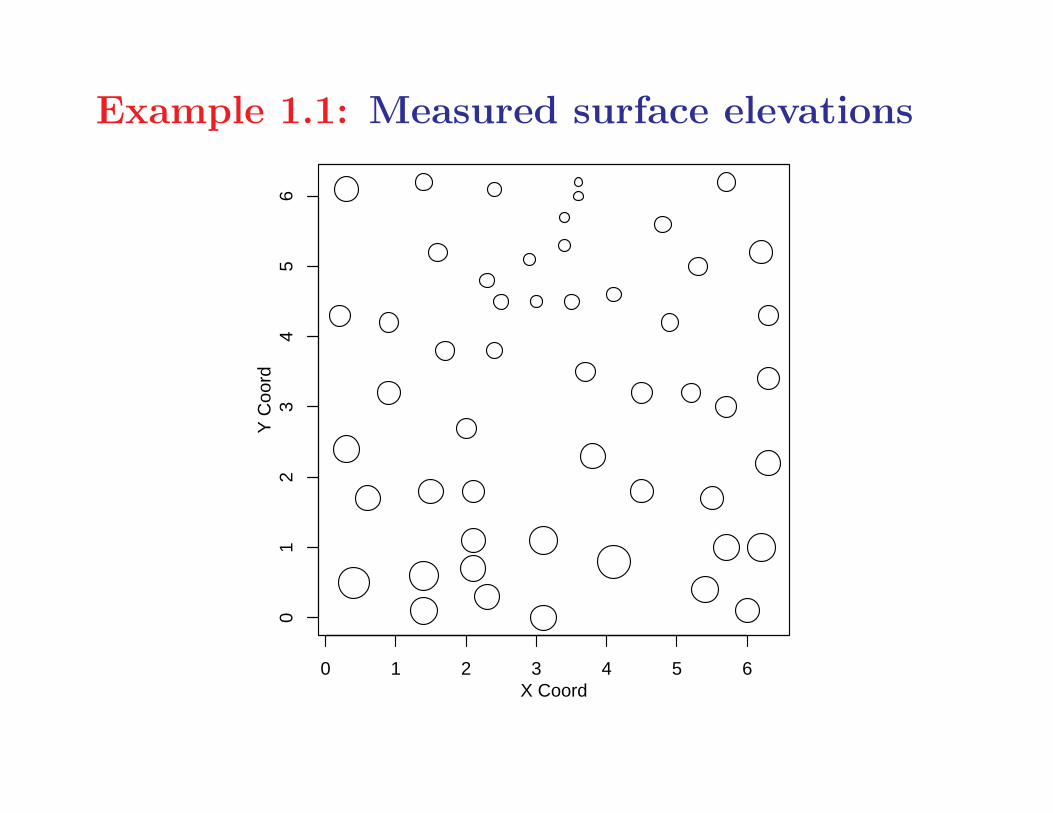
Example 1.1: Measured surface elevations
0 1 2 3 4 5 6
01
23
45
6
X Coord
Y C
oord
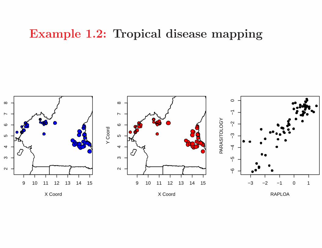
Example 1.2: Tropical disease mapping
9 10 11 12 13 14 15
23
45
67
8
X Coord
9 10 11 12 13 14 15
23
45
67
8
X Coord
Y C
oord
−3 −2 −1 0 1
−6
−5
−4
−3
−2
−1
0
RAPLOA
PAR
AS
ITO
LOG
Y
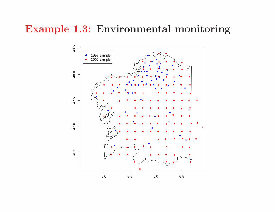
Example 1.3: Environmental monitoring
5.0 5.5 6.0 6.5
46.5
47.0
47.5
48.0
48.5
1997 sample2000 sample
Model-based Geostatistics
• the application of general principles of statisticalmodelling and inference to geostatistical problems
• Example: kriging as minimum mean square errorprediction under Gaussian modelling assumptions
Gaussian geostatistics
Model
• Stationary Gaussian process S(x) : x ∈ IR2
· E[S(x)] = µ
· Cov{S(x), S(x′)} = σ2ρ(‖x − x′‖)
• Mutually independent Yi|S(·) ∼ N(S(x), τ 2)
Point predictor S(x) = E[S(x)|Y ]
• linear in Y = (Y1, ..., Yn);
• interpolates Y if τ 2 = 0.
Parameter uncertainty?
• usually ignored in traditional geostatistics(plug-in prediction)
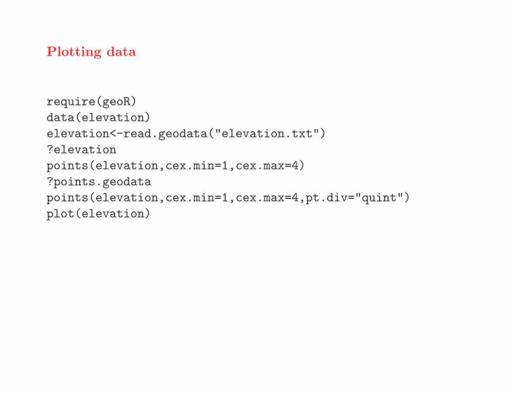
Plotting data
require(geoR)
data(elevation)
elevation<-read.geodata("elevation.txt")
?elevation
points(elevation,cex.min=1,cex.max=4)
?points.geodata
points(elevation,cex.min=1,cex.max=4,pt.div="quint")
plot(elevation)
TOPIC 2
Linear models
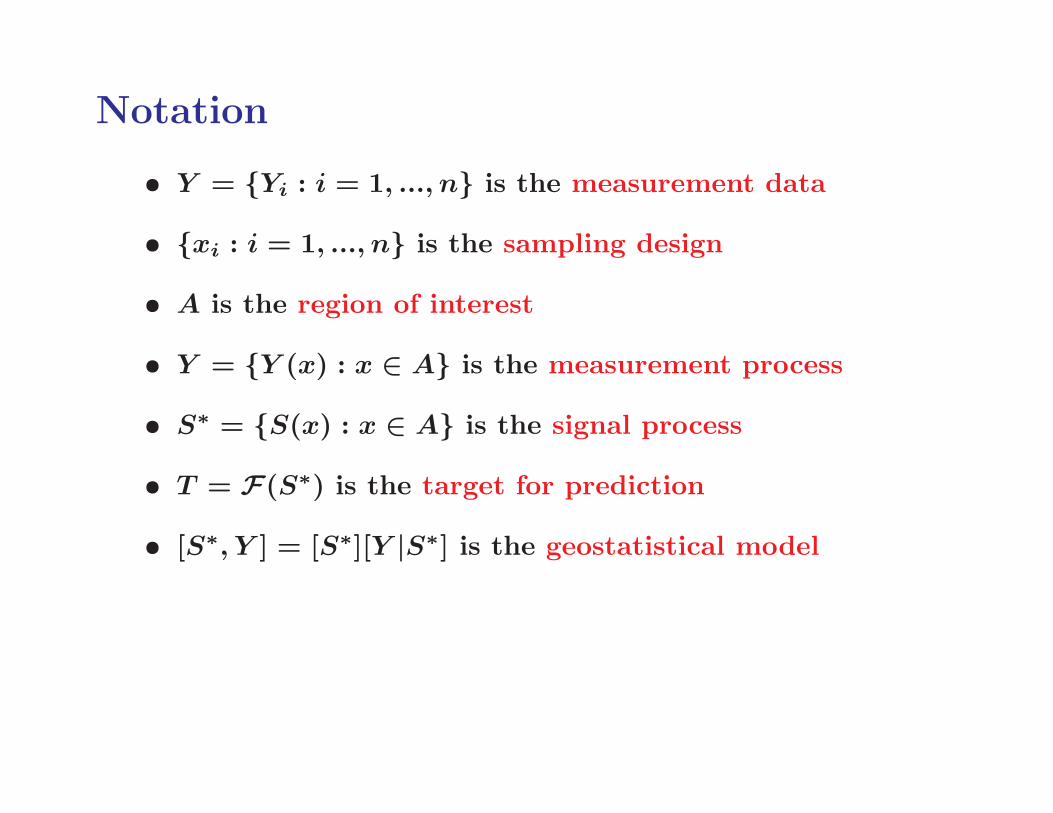
Notation
• Y = {Yi : i = 1, ..., n} is the measurement data
• {xi : i = 1, ..., n} is the sampling design
• A is the region of interest
• Y = {Y (x) : x ∈ A} is the measurement process
• S∗ = {S(x) : x ∈ A} is the signal process
• T = F(S∗) is the target for prediction
• [S∗, Y ] = [S∗][Y |S∗] is the geostatistical model
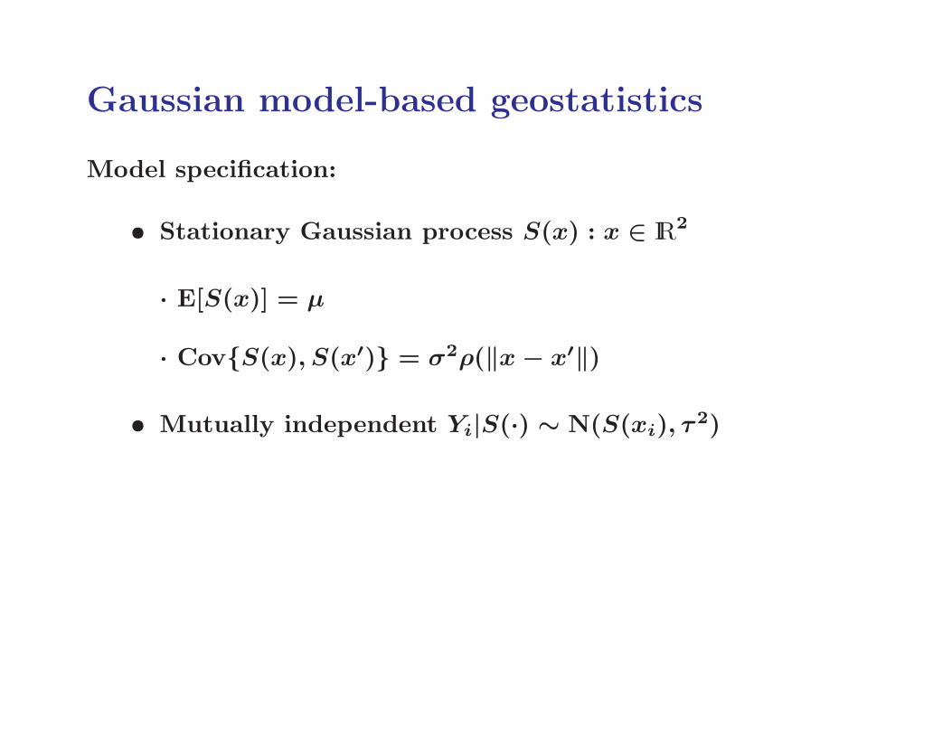
Gaussian model-based geostatistics
Model specification:
• Stationary Gaussian process S(x) : x ∈ IR2
· E[S(x)] = µ
· Cov{S(x), S(x′)} = σ2ρ(‖x − x′‖)
• Mutually independent Yi|S(·) ∼ N(S(xi), τ2)
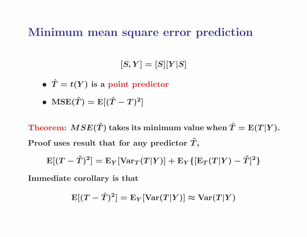
Minimum mean square error prediction
[S, Y ] = [S][Y |S]
• T = t(Y ) is a point predictor
• MSE(T ) = E[(T − T )2]
Theorem: MSE(T ) takes its minimum value when T = E(T |Y ).
Proof uses result that for any predictor T ,
E[(T − T )2] = EY [VarT (T |Y )] + EY {[ET (T |Y ) − T ]2}
Immediate corollary is that
E[(T − T )2] = EY [Var(T |Y )] ≈ Var(T |Y )
Simple and ordinary kriging
Recall Gaussian model:
• Stationary Gaussian process S(x) : x ∈ IR2
· E[S(x)] = µ
· Cov{S(x), S(x′)} = σ2ρ(‖x − x′‖)
• Mutually independent Yi|S(·) ∼ N(S(x), τ 2)
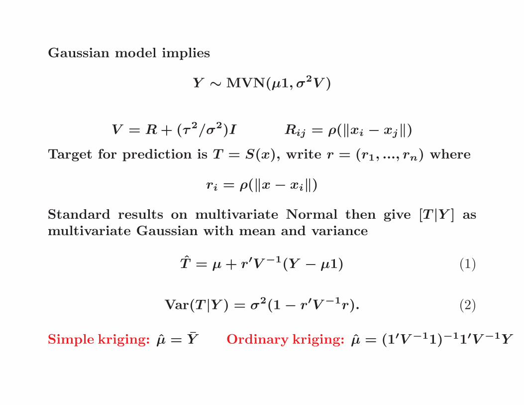
Gaussian model implies
Y ∼ MVN(µ1, σ2V )
V = R + (τ 2/σ2)I Rij = ρ(‖xi − xj‖)Target for prediction is T = S(x), write r = (r1, ..., rn) where
ri = ρ(‖x − xi‖)
Standard results on multivariate Normal then give [T |Y ] asmultivariate Gaussian with mean and variance
T = µ + r′V −1(Y − µ1) (1)
Var(T |Y ) = σ2(1 − r′V −1r). (2)
Simple kriging: µ = Y Ordinary kriging: µ = (1′V −11)−11′V −1Y
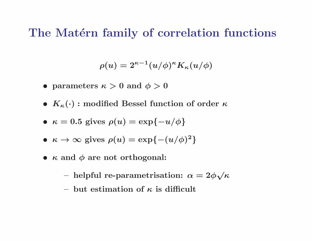
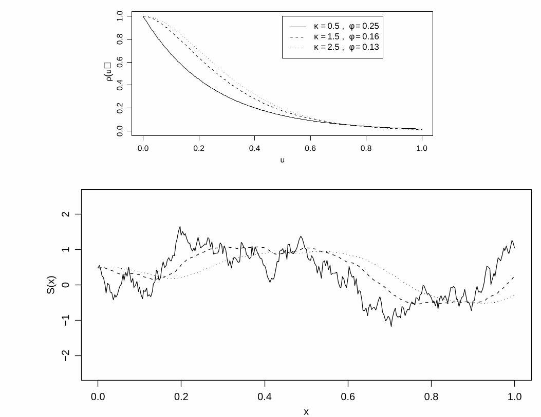
The Matern family of correlation functions
ρ(u) = 2κ−1(u/φ)κKκ(u/φ)
• parameters κ > 0 and φ > 0
• Kκ(·) : modified Bessel function of order κ
• κ = 0.5 gives ρ(u) = exp{−u/φ}
• κ → ∞ gives ρ(u) = exp{−(u/φ)2}
• κ and φ are not orthogonal:
– helpful re-parametrisation: α = 2φ√κ
– but estimation of κ is difficult
0.0 0.2 0.4 0.6 0.8 1.0
0.0
0.2
0.4
0.6
0.8
1.0
u
ρ(u)
κ = 0.5 , φ = 0.25κ = 1.5 , φ = 0.16κ = 2.5 , φ = 0.13
0.0 0.2 0.4 0.6 0.8 1.0
−2
−1
01
2
x
S(x
)
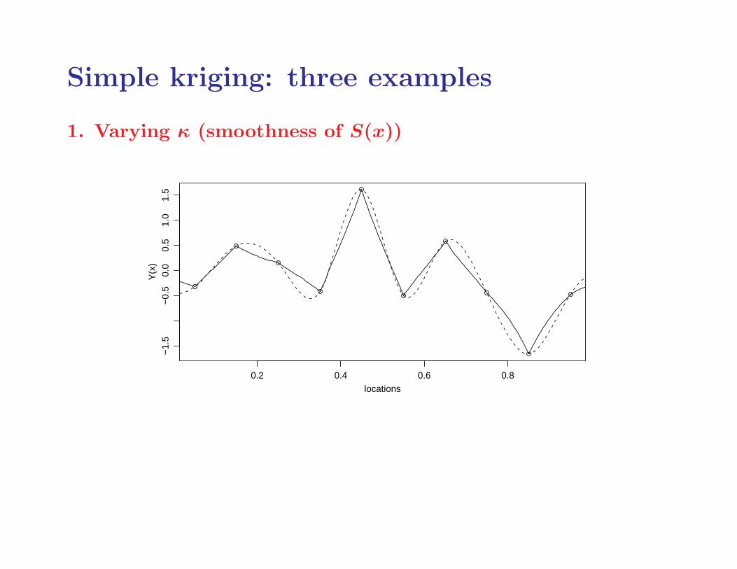
Simple kriging: three examples
1. Varying κ (smoothness of S(x))
0.2 0.4 0.6 0.8
−1.
5−
0.5
0.0
0.5
1.0
1.5
locations
Y(x
)
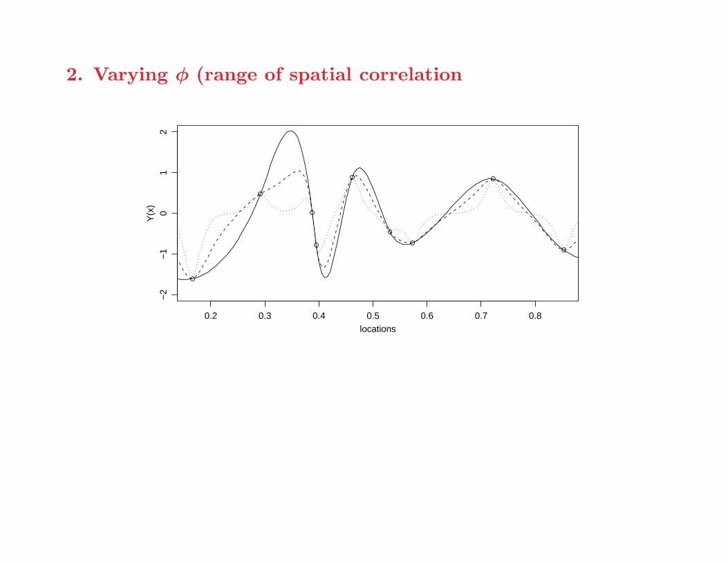
2. Varying φ (range of spatial correlation
0.2 0.3 0.4 0.5 0.6 0.7 0.8
−2
−1
01
2
locations
Y(x
)
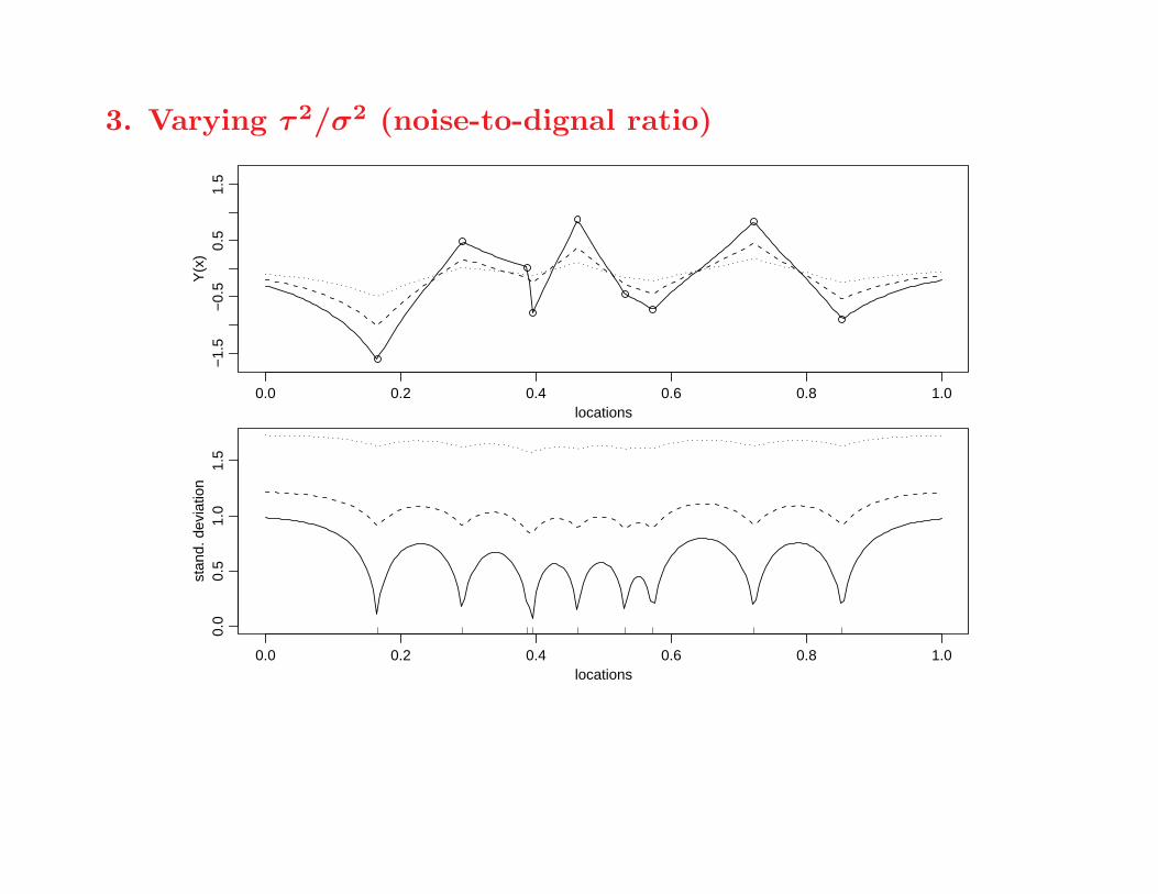
3. Varying τ 2/σ2 (noise-to-dignal ratio)
0.0 0.2 0.4 0.6 0.8 1.0
−1.
5−
0.5
0.5
1.5
locations
Y(x
)
0.0 0.2 0.4 0.6 0.8 1.0
0.0
0.5
1.0
1.5
locations
stan
d. d
evia
tion
Predicting non-linear functionals
• minimum mean square error prediction is not invariantunder non-linear transformation
• the complete answer to a prediction problem is thepredictive distribution, [T |Y ]
• Recommended strategy:
– draw repeated samples from [S∗|Y ](conditional simulation)
– calculate required summaries(examples to follow)
Theoretical variograms
• the variogram of a process Y (x) is the function
V (x, x′) =1
2Var{Y (x) − Y (x′)}
• for the spatial Gaussian model, with u = ||x − x′||,
V (u) = τ 2 + σ2{1 − ρ(u)}
• provides a summary of the basic structural parametersof the spatial Gaussian process
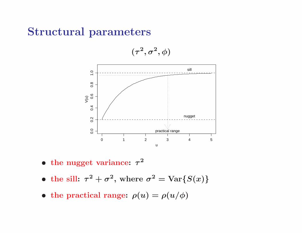
Structural parameters
(τ 2, σ2, φ)
0 1 2 3 4 5
0.0
0.2
0.4
0.6
0.8
1.0
u
V(u
)
sill
nugget
practical range
• the nugget variance: τ 2
• the sill: τ 2 + σ2, where σ2 = Var{S(x)}
• the practical range: ρ(u) = ρ(u/φ)
Empirical variograms
uij = ‖xi − xj‖ vij = 0.5[y(xi) − y(xj)]2
• the variogram cloud is a scatterplot of the points (uij , vij)
• the empirical variogram smooths the variogram cloud byaveraging within bins: u − h/2 ≤ uij < u + h/2
• for a process with non-constant mean (covariates), useresiduals r(xi) = y(xi) − µ(xi) to compute vij
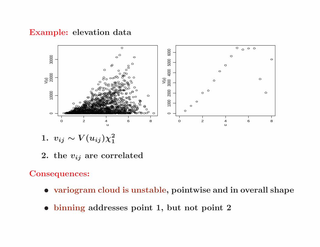
Example: elevation data
0 2 4 6 8
010
000
2000
030
000
u
V(u)
0 2 4 6 8
010
0020
0030
0040
0050
0060
00
u
V(u)
1. vij ∼ V (uij)χ2
1
2. the vij are correlated
Consequences:
• variogram cloud is unstable, pointwise and in overall shape
• binning addresses point 1, but not point 2

Calculating an empirical variogram
vario1<-variog(elevation,uvec=0.5*(0:10))
plot(vario1)
plot(vario1,pch=19,col="red")
?variog
vario2<-variog(elevation,uvec=0.5*(0:10),trend="2nd")
plot(vario2)
names(vario1)
plot(vario1$u,vario1$v,type="l",xlim=c(0,5),ylim=c(0,6500),
xlab="u",ylab="V(u)")
lines(vario2$u,vario2$v,col="red")
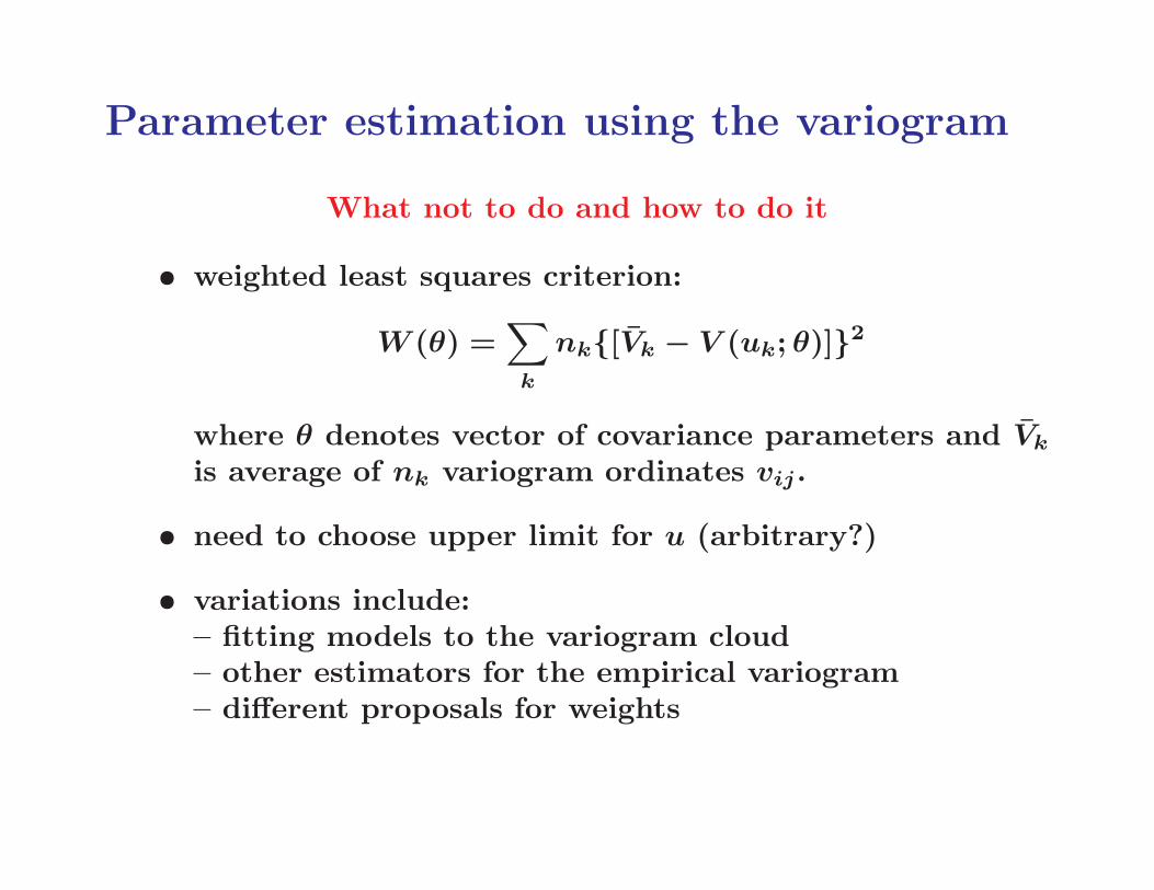
Parameter estimation using the variogram
What not to do and how to do it
• weighted least squares criterion:
W (θ) =∑
k
nk{[Vk − V (uk; θ)]}2
where θ denotes vector of covariance parameters and Vk
is average of nk variogram ordinates vij.
• need to choose upper limit for u (arbitrary?)
• variations include:– fitting models to the variogram cloud– other estimators for the empirical variogram– different proposals for weights
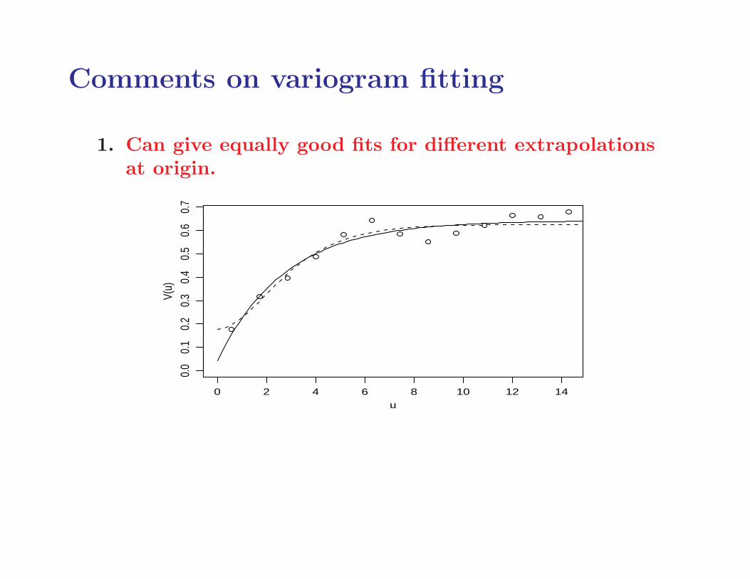
Comments on variogram fitting
1. Can give equally good fits for different extrapolationsat origin.
0 2 4 6 8 10 12 14
0.0
0.1
0.2
0.3
0.4
0.5
0.6
0.7
u
V(u)
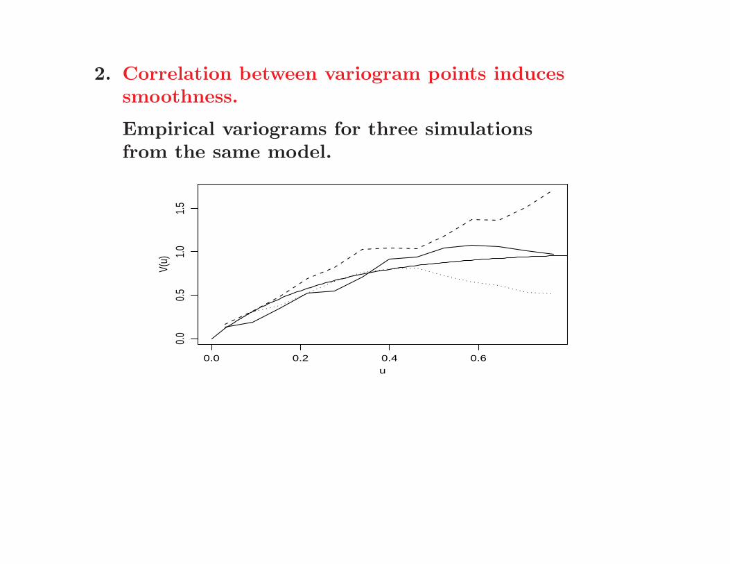
2. Correlation between variogram points inducessmoothness.
Empirical variograms for three simulationsfrom the same model.
0.0 0.2 0.4 0.6
0.0
0.5
1.0
1.5
u
V(u)
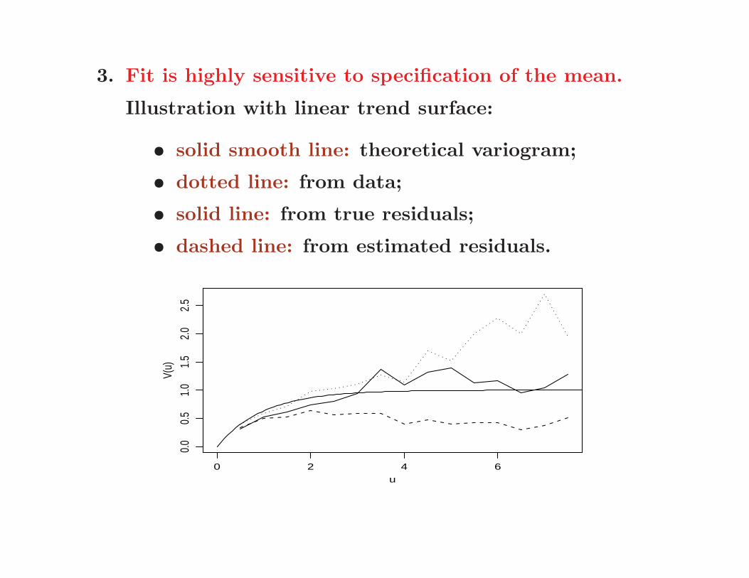
3. Fit is highly sensitive to specification of the mean.
Illustration with linear trend surface:
• solid smooth line: theoretical variogram;
• dotted line: from data;
• solid line: from true residuals;
• dashed line: from estimated residuals.
0 2 4 6
0.0
0.5
1.0
1.5
2.0
2.5
u
V(u)
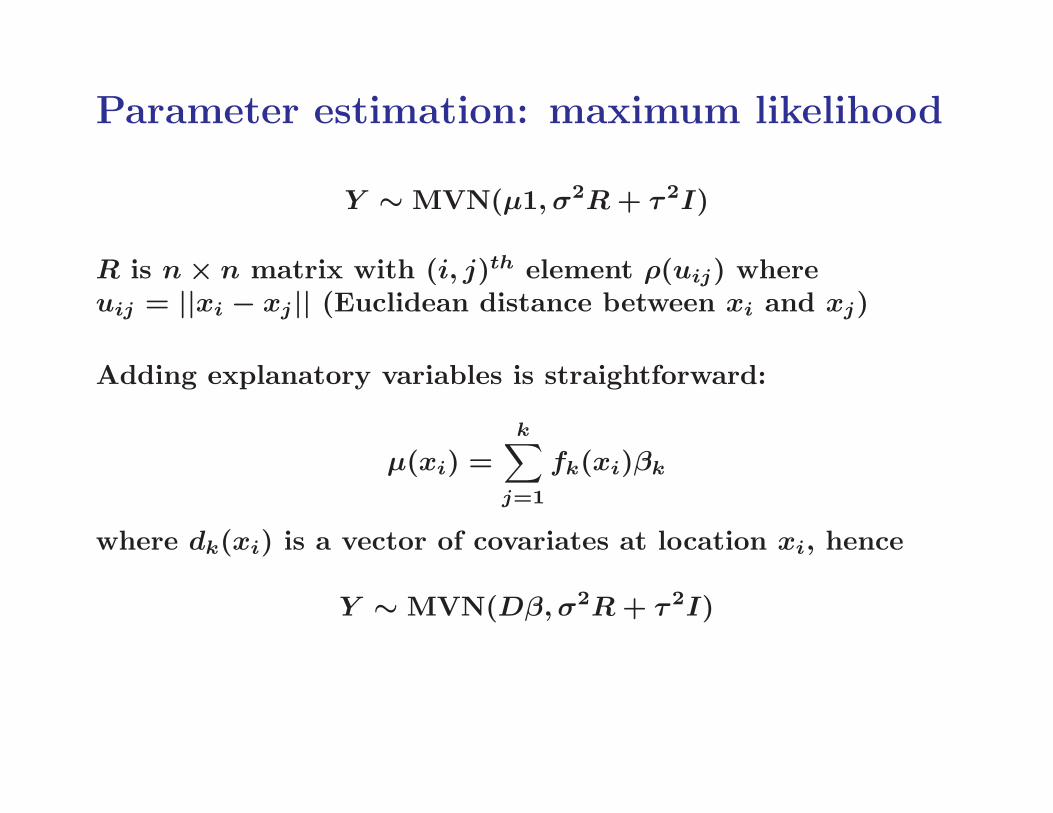
Parameter estimation: maximum likelihood
Y ∼ MVN(µ1, σ2R + τ 2I)
R is n × n matrix with (i, j)th element ρ(uij) whereuij = ||xi − xj || (Euclidean distance between xi and xj)
Adding explanatory variables is straightforward:
µ(xi) =k∑
j=1
fk(xi)βk
where dk(xi) is a vector of covariates at location xi, hence
Y ∼ MVN(Dβ,σ2R + τ 2I)

Gaussian log-likelihood function
Y ∼ MVN(Dβ,σ2R + τ 2I)
• write ν2 = τ 2/σ2, hence σ2V = σ2(R + ν2I)
• log-likelihood function is maximised for
β(V ) = (D′V −1D)−1D′V −1y
σ2 = n−1(y − Dβ)′V −1(y − Dβ)
• substitute (β, σ2) to give reduced maximisation problem
L∗(ν2, φ, κ) ∝ −0.5{n log |σ2| + log |(R + ν2I)|}
In practice, choose κ from a discrete set, e.g. κ = 0.5, 1, 2
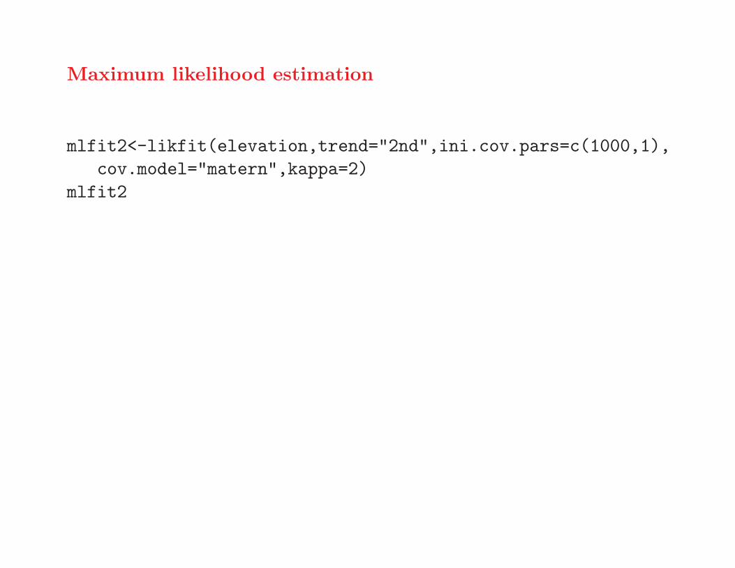
Maximum likelihood estimation
mlfit2<-likfit(elevation,trend="2nd",ini.cov.pars=c(1000,1),
cov.model="matern",kappa=2)
mlfit2
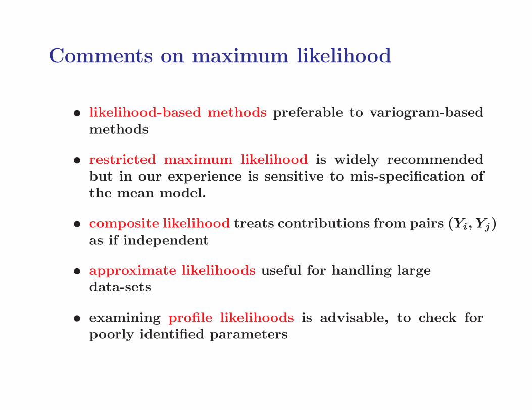
Comments on maximum likelihood
• likelihood-based methods preferable to variogram-basedmethods
• restricted maximum likelihood is widely recommendedbut in our experience is sensitive to mis-specification ofthe mean model.
• composite likelihood treats contributions from pairs (Yi, Yj)as if independent
• approximate likelihoods useful for handling largedata-sets
• examining profile likelihoods is advisable, to check forpoorly identified parameters
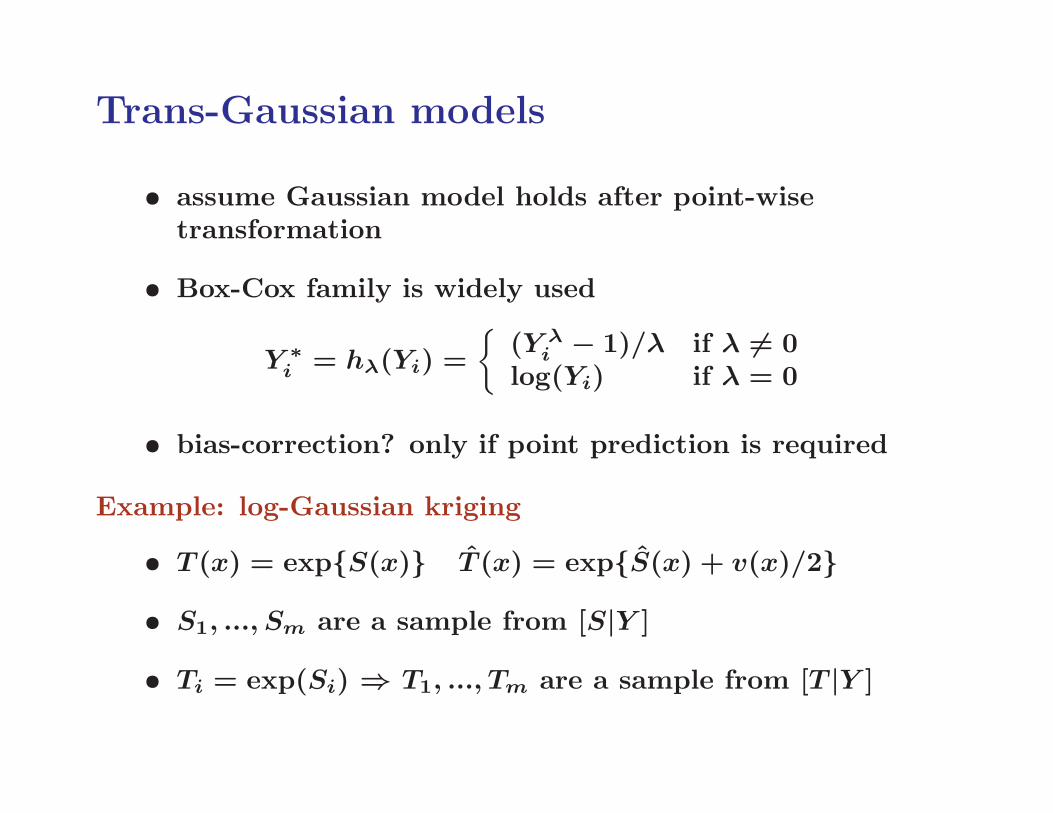
Trans-Gaussian models
• assume Gaussian model holds after point-wisetransformation
• Box-Cox family is widely used
Y ∗i = hλ(Yi) =
{
(Y λi − 1)/λ if λ 6= 0
log(Yi) if λ = 0
• bias-correction? only if point prediction is required
Example: log-Gaussian kriging
• T (x) = exp{S(x)} T (x) = exp{S(x) + v(x)/2}
• S1, ..., Sm are a sample from [S|Y ]
• Ti = exp(Si) ⇒ T1, ..., Tm are a sample from [T |Y ]
Plug-in prediction
region<-matrix(c(0,0,6.5,0,6.5,6.5,0,6.5),4,2,T)
grid<-as.matrix(pred_grid(region,by=0.25))
KC<-krige.control(obj.model=mlfit2,trend.d="2nd",trend.l="2nd")
OC<-output.control(n.predictive=100)
set.seed(24367)
predictions<-krige.conv(geodata=elevation,locations=grid,
borders=region,krige=KC,output=OC)
image(predictions)
points(elevation,add=T)
par(mfrow=c(1,2))
hist(elevation$data,main="data")
predict.max<-NULL
for (sim in 1:100) {
predict.max<-c(predict.max,max(predictions$simulations[,sim]))
}
hist(predict.max,main="predicted maximum")
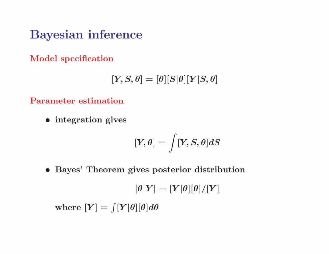
Bayesian inference
Model specification
[Y, S, θ] = [θ][S|θ][Y |S, θ]
Parameter estimation
• integration gives
[Y, θ] =
∫
[Y, S, θ]dS
• Bayes’ Theorem gives posterior distribution
[θ|Y ] = [Y |θ][θ]/[Y ]
where [Y ] =∫
[Y |θ][θ]dθ
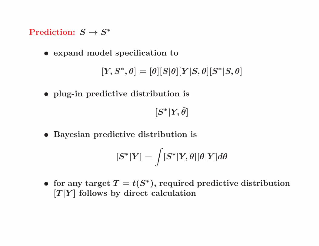
Prediction: S → S∗
• expand model specification to
[Y, S∗, θ] = [θ][S|θ][Y |S, θ][S∗|S, θ]
• plug-in predictive distribution is
[S∗|Y, θ]
• Bayesian predictive distribution is
[S∗|Y ] =
∫
[S∗|Y, θ][θ|Y ]dθ
• for any target T = t(S∗), required predictive distribution[T |Y ] follows by direct calculation
Notes
• likelihood function is central to both classical and Bayesianinference
• Bayesian prediction is a weighted average of plug-inpredictions, with different plug-in values of θweighted according to their conditional probabilitiesgiven the observed data.
• Bayesian prediction is usually more conservativethan plug-in prediction
• Sampling from posterior and predictive distributions usesdirect Monte Carlo:
– conjugate priors for mean and variance parameters
– discrete priors for covariance parameters
Bayesian estimation and prediction
MC<-model.control(trend.d="2nd",trend.l="2nd",kappa=2)
PC<-prior.control(beta.prior="flat",sigmasq.prior="sc.inv.chisq",
sigmasq=1000,df.sigmasq=4,phi.discrete=0.5*(1:5),
tausq.rel.prior="uniform",tausq.rel.discrete=0.1*(1:5))
OC<-output.control(n.posterior=100,n.predictive=100,
simulations.predictive=T,signal=T,moments=F)
set.seed(24367)
results.bayes<-krige.bayes(geodata=elevation,locations=grid,
borders=region,model=MC,prior=PC,output=OC)
Plotting posterior distributions
plot(results.bayes)
posteriors.bayes<-results.bayes$posterior
posterior.sample<-posteriors.bayes$sample
par(mfrow=c(3,3))
for (i in 1:9) {
hist(posterior.sample[,i],main=" ")
}
par(mfrow=c(1,1))
plot(posterior.sample[,2],posterior.sample[,3])
Plotting predictive distributions
predictions.bayes<-results.bayes$predictive
image(unique(grid[,1]),unique(grid[,2]),
matrix(predictions.bayes$mean.simulations,27,27))
points(elevation,add=T)
par(mfrow=c(1,2))
predict.max<-NULL
for (sim in 1:100) {
predict.max<-c(predict.max,max(predictions$simulations[,sim]))
}
hist(predict.max,xlab="maximum", main="plug-in")
predict.bayes.max<-NULL
for (sim in 1:100) {
predict.bayes.max<-c(predict.bayes.max,
max(predictions.bayes$simulations[,sim]))
}
hist(predict.bayes.max,xlab="maximum",main="Bayesian")
TOPIC 3
Generalized linear models

AfricanProgramme forOnchocerciasisControl
• “river blindness” – an endemic disease in wet tropicalregions
• donation programme of mass treatment with ivermectin
• approximately 30 million treatments to date
• serious adverse reactions experienced by some patientshighly co-infected with Loa loa parasites
• precautionary measures put in place before masstreatment in areas of high Loa loa prevalence
http://www.who.int/pbd/blindness/onchocerciasis/en/
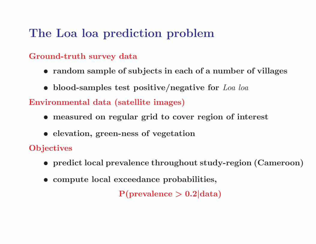
The Loa loa prediction problem
Ground-truth survey data
• random sample of subjects in each of a number of villages
• blood-samples test positive/negative for Loa loa
Environmental data (satellite images)
• measured on regular grid to cover region of interest
• elevation, green-ness of vegetation
Objectives
• predict local prevalence throughout study-region (Cameroon)
• compute local exceedance probabilities,
P(prevalence > 0.2|data)
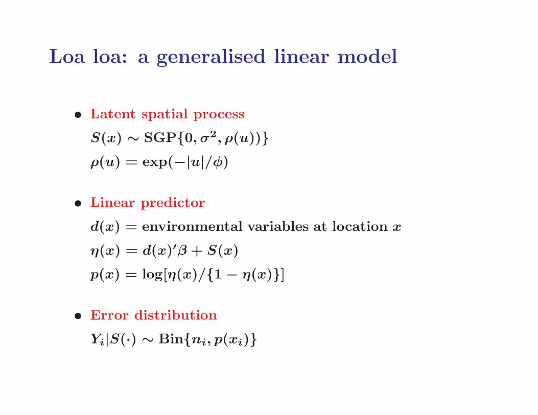
Loa loa: a generalised linear model
• Latent spatial process
S(x) ∼ SGP{0, σ2, ρ(u))}ρ(u) = exp(−|u|/φ)
• Linear predictor
d(x) = environmental variables at location x
η(x) = d(x)′β + S(x)
p(x) = log[η(x)/{1 − η(x)}]
• Error distribution
Yi|S(·) ∼ Bin{ni, p(xi)}
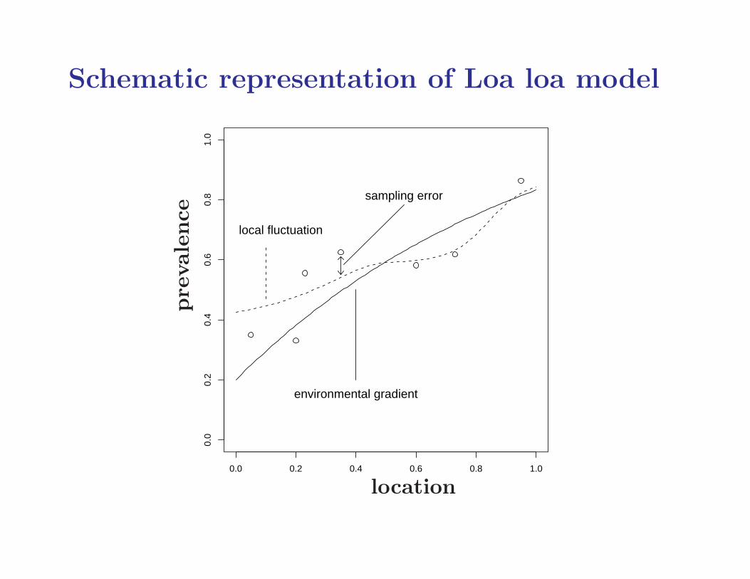
Schematic representation of Loa loa model
0.0 0.2 0.4 0.6 0.8 1.0
0.0
0.2
0.4
0.6
0.8
1.0
environmental gradient
local fluctuation
sampling errorprevalence
location
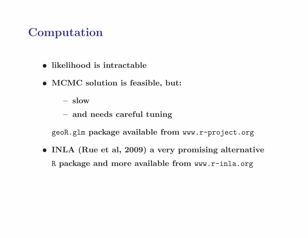
Computation
• likelihood is intractable
• MCMC solution is feasible, but:
– slow
– and needs careful tuning
geoR.glm package available from www.r-project.org
• INLA (Rue et al, 2009) a very promising alternative
R package and more available from www.r-inla.org
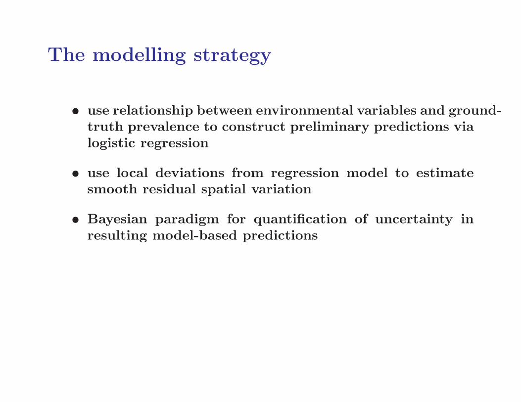
The modelling strategy
• use relationship between environmental variables and ground-truth prevalence to construct preliminary predictions vialogistic regression
• use local deviations from regression model to estimatesmooth residual spatial variation
• Bayesian paradigm for quantification of uncertainty inresulting model-based predictions
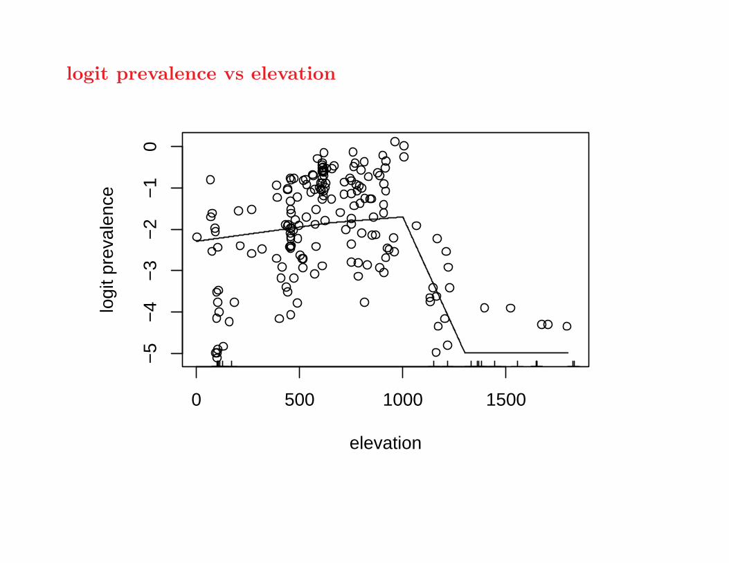
logit prevalence vs elevation
0 500 1000 1500
−5
−4
−3
−2
−1
0
elevation
logi
t pre
vale
nce
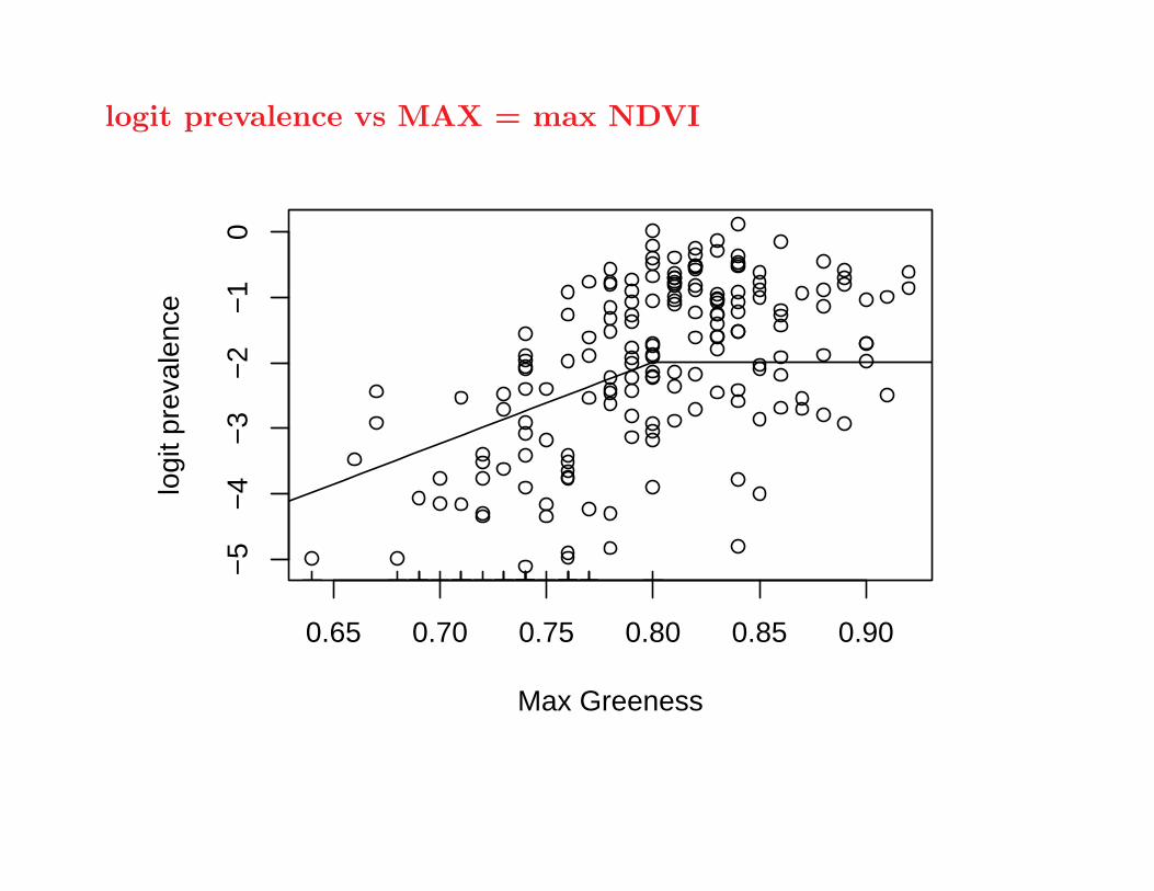
logit prevalence vs MAX = max NDVI
0.65 0.70 0.75 0.80 0.85 0.90
−5
−4
−3
−2
−1
0
Max Greeness
logi
t pre
vale
nce
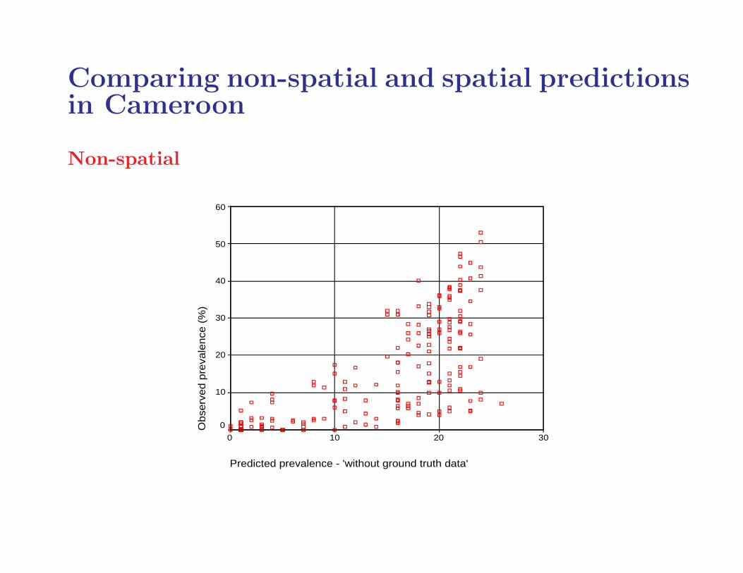
Comparing non-spatial and spatial predictionsin Cameroon
Non-spatial
Predicted prevalence - 'without ground truth data'
3020100
Obse
rved p
reva
lence
(%
)60
50
40
30
20
10
0
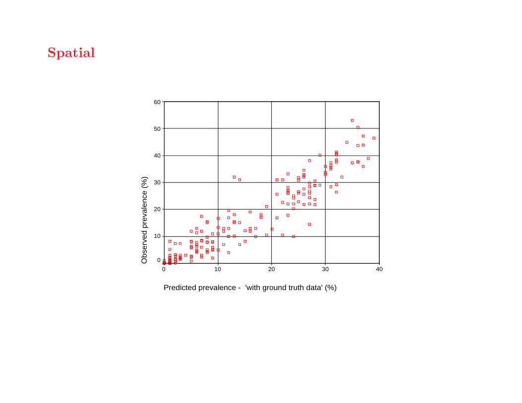
Spatial
Predicted prevalence - 'with ground truth data' (%)
403020100
Obs
erve
d pr
eval
ence
(%
)
60
50
40
30
20
10
0
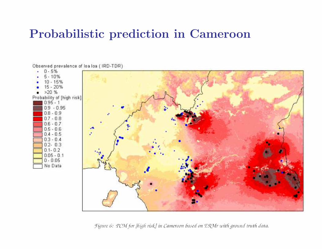
Probabilistic prediction in Cameroon

Next Steps
• analysis confirms value of local ground-truth prevalencedata
• in some areas, need more ground-truth data to reducepredictive uncertainty
• but parasitological surveys are expensive

Field-work is difficult!
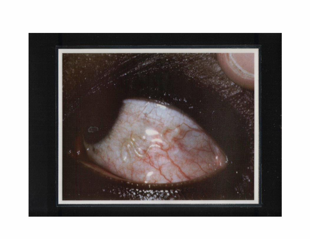
RAPLOA
• a cheaper alternative to parasitological sampling:
– have you ever experienced eye-worm?
– did it look like this photograph?
– did it go away within a week?
• RAPLOA data to be collected:
– in sample of villages previously surveyedparasitologically (to calibrate parasitology vs RAPLOAestimates)
– in villages not surveyed parasitologically (to reducelocal uncertainty)
• bivariate model needed for combined analysis ofparasitological and RAPLOA prevalence estimates

UNDP/World Bank/WHO Special Programme for Research & Training in Tropical Disease (TDR)
R E P O RT O F A M U LT I - C E N T R E S T U DY
Rapid AssessmentProceduresfor Loiasis
TDR/IDE/RP/RAPL/01.1
catio
n
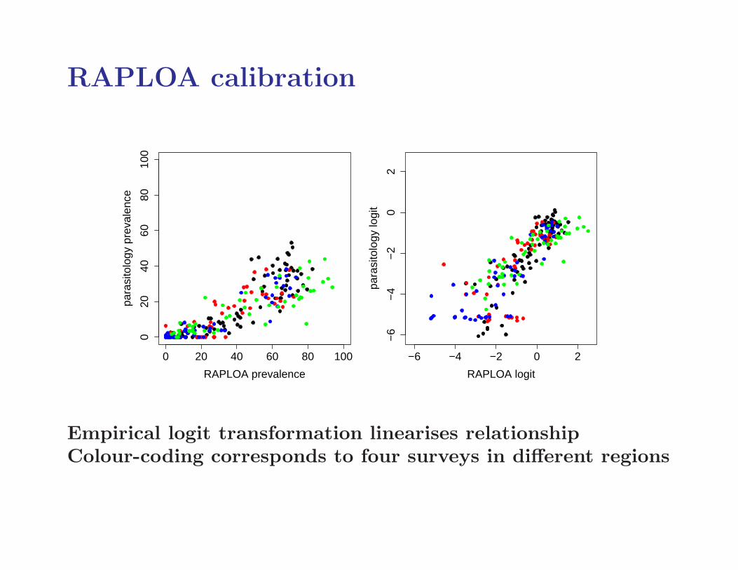
RAPLOA calibration
0 20 40 60 80 100
020
4060
8010
0
RAPLOA prevalence
para
sito
logy
pre
vale
nce
−6 −4 −2 0 2
−6
−4
−2
02
RAPLOA logitpa
rasi
tolo
gy lo
git
locatio
n
Empirical logit transformation linearises relationshipColour-coding corresponds to four surveys in different regions
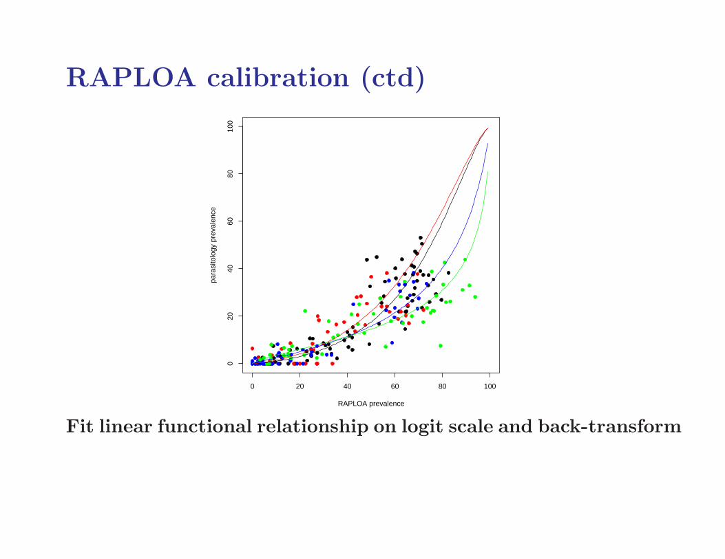
RAPLOA calibration (ctd)
0 20 40 60 80 100
020
4060
8010
0
RAPLOA prevalence
para
sito
logy
pre
vale
nce
Fit linear functional relationship on logit scale and back-transform
RAPLOA mapping: methodology
1. use geostatistical model to draw samples from predictivedistribution of logit-transformed RAPLOA prevalence
2. use calibration model to draw samples from predictivedistribution of logit-transformed parasitological prevalenceconditional on RAPLOA prevalence
3. back-transform to parasitological prevalence
4. map empirical exceedance proportions at each location
Method ensures correct propagation of uncertaintyat each stage
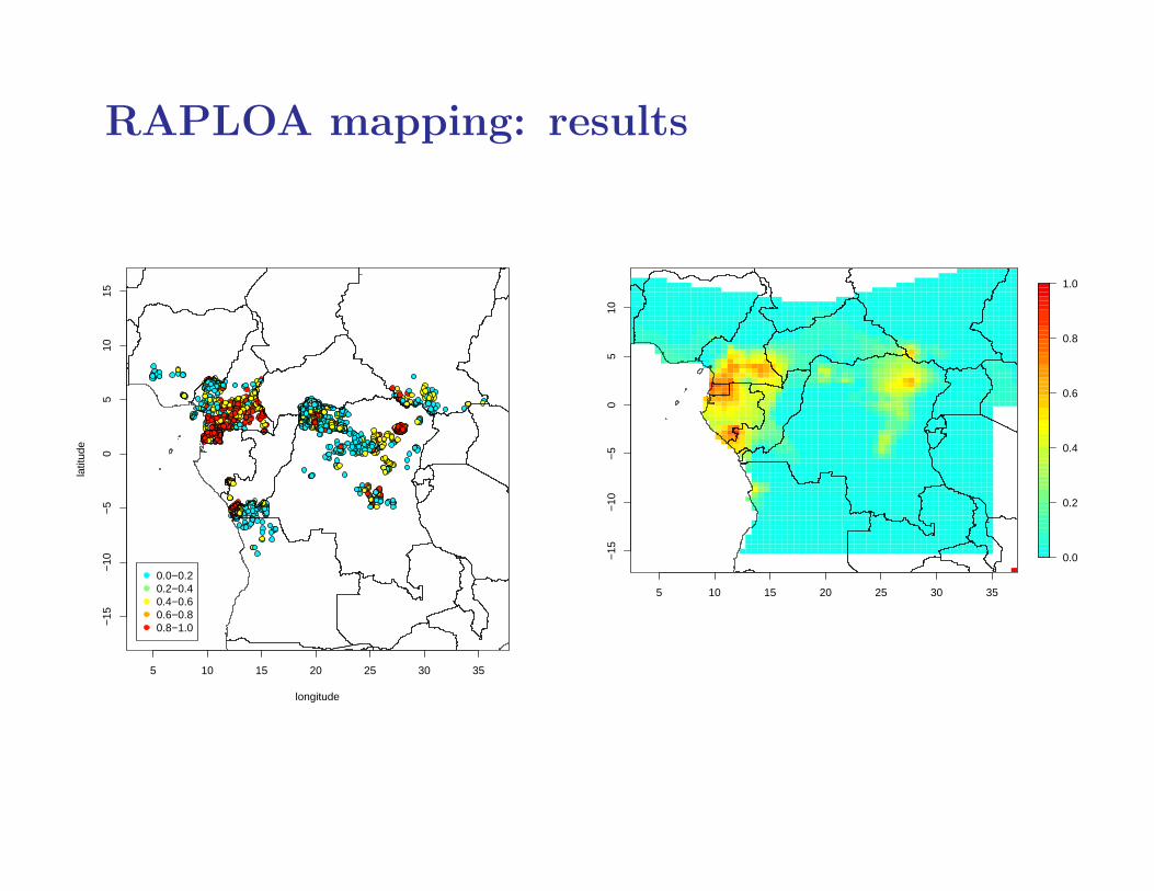
RAPLOA mapping: results
5 10 15 20 25 30 35
−15
−10
−5
05
1015
longitude
latit
ude
0.0−0.20.2−0.40.4−0.60.6−0.80.8−1.0
5 10 15 20 25 30 35
−15
−10
−5
05
10
0.0
0.2
0.4
0.6
0.8
1.0

TOPIC 4
Geostatistical design
Geostatistical design
• Retrospective
Add to, or delete from, an existing set of measurementlocations xi ∈ A : i = 1, ..., n.
• Prospective
Choose optimal positions for a new set of measurementlocations xi ∈ A : i = 1, ..., n.

Naive design folklore
• Spatial correlation decreases with increasing distance.
• Therefore, close pairs of points are wasteful.
• Therefore, spatially regular designs are a good thing.
Less naive design folklore
• Spatial correlation decreases with increasing distance.
• Therefore, close pairs of points are wasteful if you knowthe correct model.
• But in practice, at best, you need to estimate unknownmodel parameters.
• And to estimate model parameters, you need your designto include a wide range of inter-point distances.
• Therefore, spatially regular designs should be temperedby the inclusion of some close pairs of points.

Examples of compromise designs
0 1
0
1
A) Lattice plus close pairs design
0 1
0
1
B) Lattice plus in−fill design
Further remarks on geostatistical design
1. Conceptually more complex problems include:
(a) design when some sub-areas are more interestingthan others;
(b) design for best prediction of non-linear functionalsof S(·);
(c) multi-stage designs (see next session).
2. Theoretically optimal designs may not be practicable(eg Loa loa photo).
3. A more realistic goal is to suggest constructions for good,general-purpose designs.

TOPIC 5
Preferential sampling
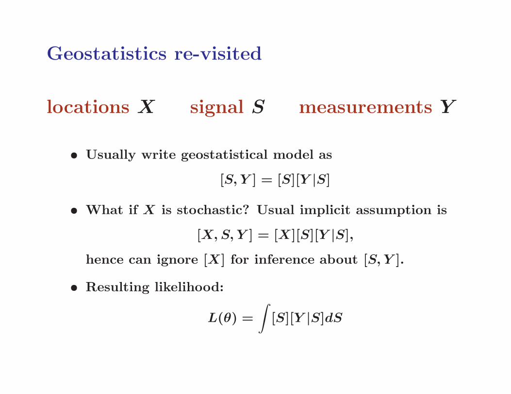
Geostatistics re-visited
locations X signal S measurements Y
• Usually write geostatistical model as
[S, Y ] = [S][Y |S]
• What if X is stochastic? Usual implicit assumption is
[X,S, Y ] = [X][S][Y |S],hence can ignore [X] for inference about [S, Y ].
• Resulting likelihood:
L(θ) =
∫
[S][Y |S]dS
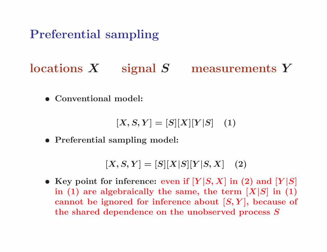
Preferential sampling
locations X signal S measurements Y
• Conventional model:
[X,S, Y ] = [S][X][Y |S] (1)
• Preferential sampling model:
[X,S, Y ] = [S][X|S][Y |S,X] (2)
• Key point for inference: even if [Y |S,X] in (2) and [Y |S]in (1) are algebraically the same, the term [X|S] in (1)cannot be ignored for inference about [S, Y ], because ofthe shared dependence on the unobserved process S
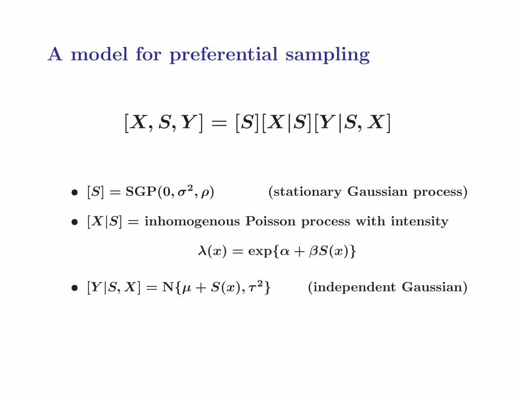
A model for preferential sampling
[X,S, Y ] = [S][X|S][Y |S,X]
• [S] = SGP(0, σ2, ρ) (stationary Gaussian process)
• [X|S] = inhomogenous Poisson process with intensity
λ(x) = exp{α + βS(x)}
• [Y |S,X] = N{µ + S(x), τ 2} (independent Gaussian)
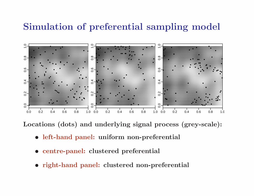
Simulation of preferential sampling model
0.0 0.2 0.4 0.6 0.8 1.0
0.0
0.2
0.4
0.6
0.8
1.0
Y C
oord
0.0 0.2 0.4 0.6 0.8 1.0
0.0
0.2
0.4
0.6
0.8
1.0
Y C
oord
0.0 0.2 0.4 0.6 0.8 1.0
0.0
0.2
0.4
0.6
0.8
1.0
Y C
oord
Locations (dots) and underlying signal process (grey-scale):
• left-hand panel: uniform non-preferential
• centre-panel: clustered preferential
• right-hand panel: clustered non-preferential
Likelihood inference
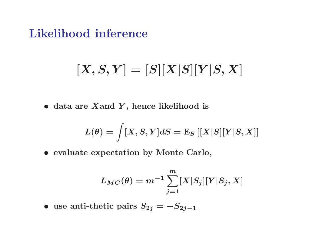
[X,S, Y ] = [S][X|S][Y |S,X]
• data are Xand Y , hence likelihood is
L(θ) =
∫
[X,S, Y ]dS = ES [[X|S][Y |S,X]]
• evaluate expectation by Monte Carlo,
LMC(θ) = m−1
m∑
j=1
[X|Sj ][Y |Sj, X]
• use anti-thetic pairs S2j = −S2j−1
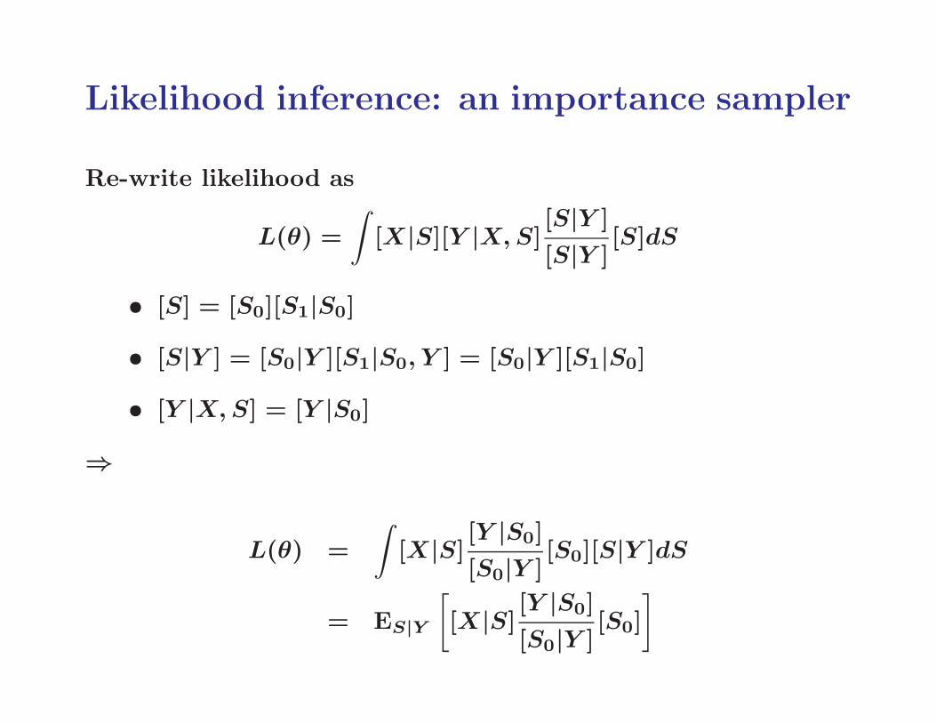
Likelihood inference: an importance sampler
Re-write likelihood as
L(θ) =
∫
[X|S][Y |X,S][S|Y ]
[S|Y ][S]dS
• [S] = [S0][S1|S0]
• [S|Y ] = [S0|Y ][S1|S0, Y ] = [S0|Y ][S1|S0]
• [Y |X,S] = [Y |S0]
⇒
L(θ) =
∫
[X|S] [Y |S0]
[S0|Y ][S0][S|Y ]dS
= ES|Y
[
[X|S] [Y |S0]
[S0|Y ][S0]
]
Practical solutions to weak identifability
1. Strong Bayesian priors (if you can believe them)
2. Explanatory variables as surrogate for S
3. Two-stage sampling
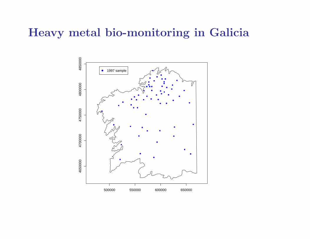
Heavy metal bio-monitoring in Galicia
500000 550000 600000 650000
4650
000
4700
000
4750
000
4800
000
4850
000
1997 sample
alence
Heavy metal bio-monitoring in Galicia
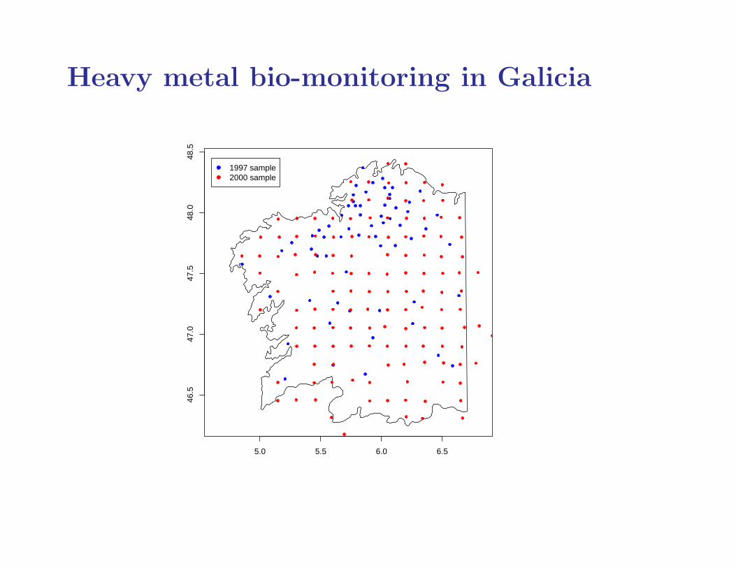
5.0 5.5 6.0 6.5
46.5
47.0
47.5
48.0
48.5
1997 sample2000 sample
alence
Heavy metal bio-monitoring in Galicia
• 1997 sampling design highly non-uniform
• may lead to biased estimates of residual spatial variation
• 2000 sampling design better for fitting model of residualspatial variation
• possible modelling framework is:
– 2000 sampling is non-preferential
– 1997 sampling may be preferential
– some parameters in common between 1997 and 2000
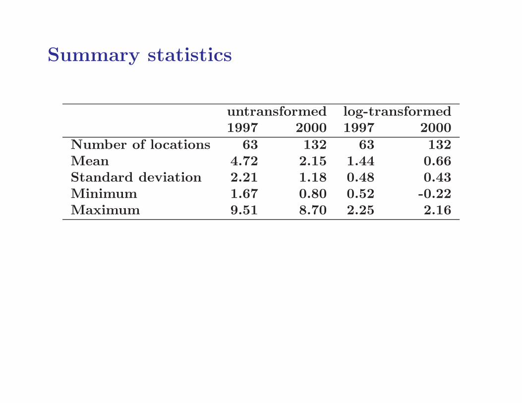
Summary statistics
untransformed log-transformed1997 2000 1997 2000
Number of locations 63 132 63 132Mean 4.72 2.15 1.44 0.66Standard deviation 2.21 1.18 0.48 0.43Minimum 1.67 0.80 0.52 -0.22Maximum 9.51 8.70 2.25 2.16
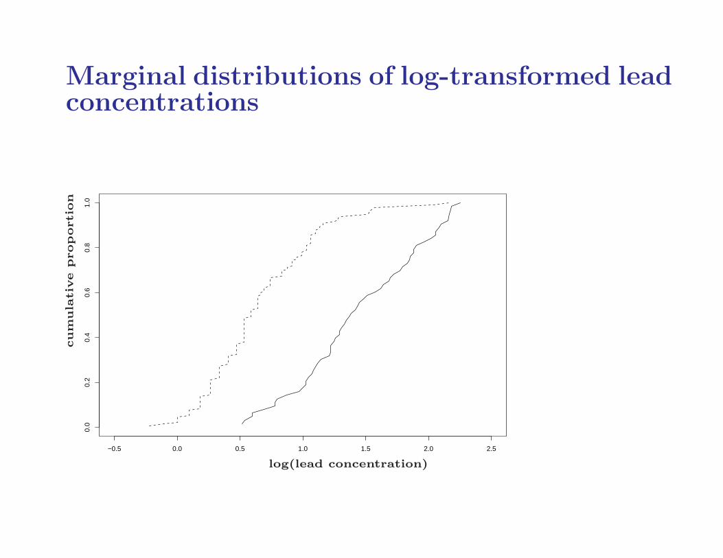
Marginal distributions of log-transformed leadconcentrations
−0.5 0.0 0.5 1.0 1.5 2.0 2.5
0.0
0.2
0.4
0.6
0.8
1.0
ts
log(lead concentration)
cum
ula
tiv
eproportio
n
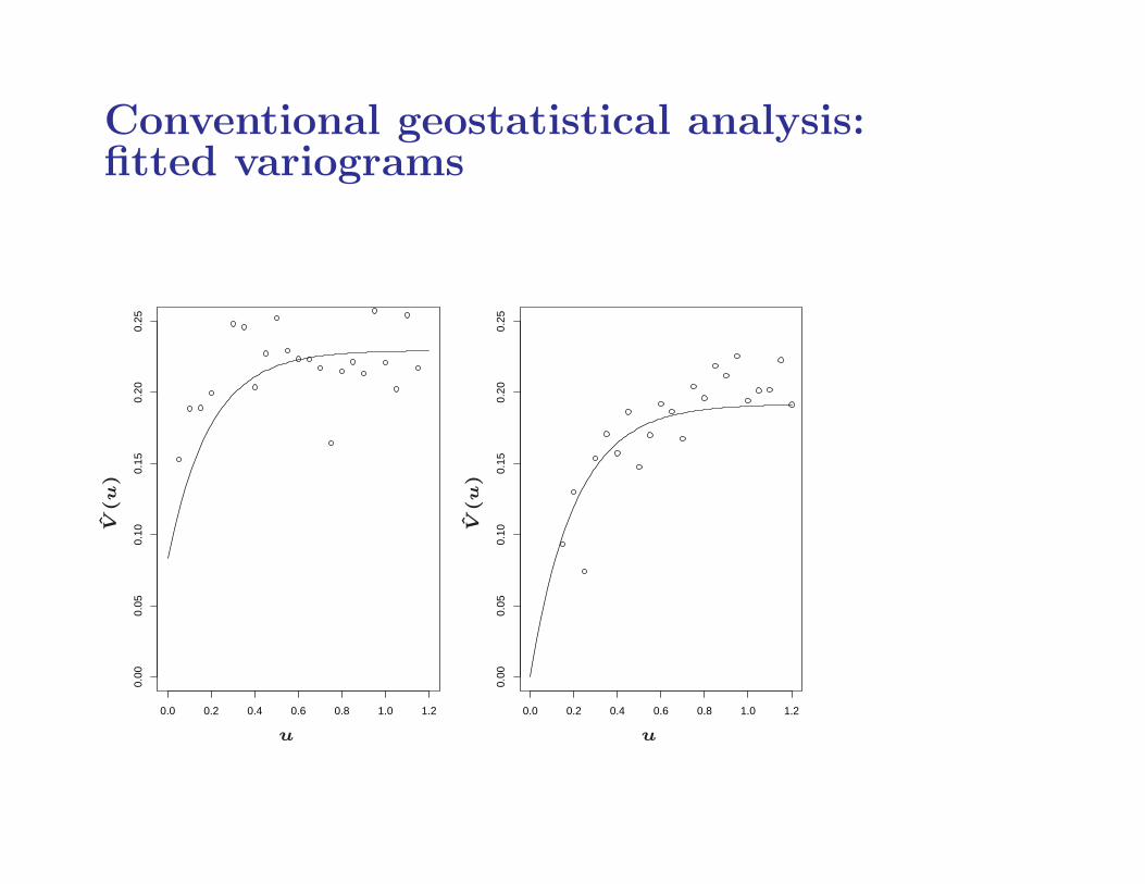
Conventional geostatistical analysis:fitted variograms
0.0 0.2 0.4 0.6 0.8 1.0 1.2
0.00
0.05
0.10
0.15
0.20
0.25
0.0 0.2 0.4 0.6 0.8 1.0 1.2
0.00
0.05
0.10
0.15
0.20
0.25
catio
n
uu
V(u)
V(u)
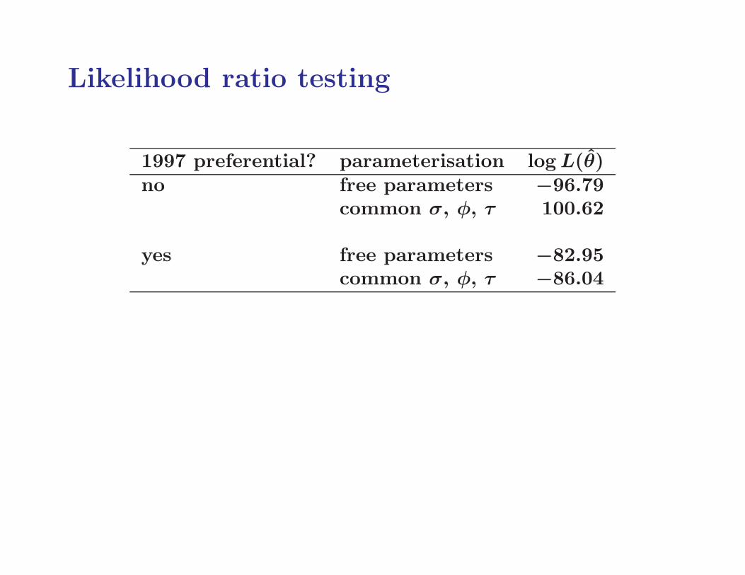
Likelihood ratio testing
1997 preferential? parameterisation logL(θ)no free parameters −96.79
common σ, φ, τ 100.62
yes free parameters −82.95common σ, φ, τ −86.04
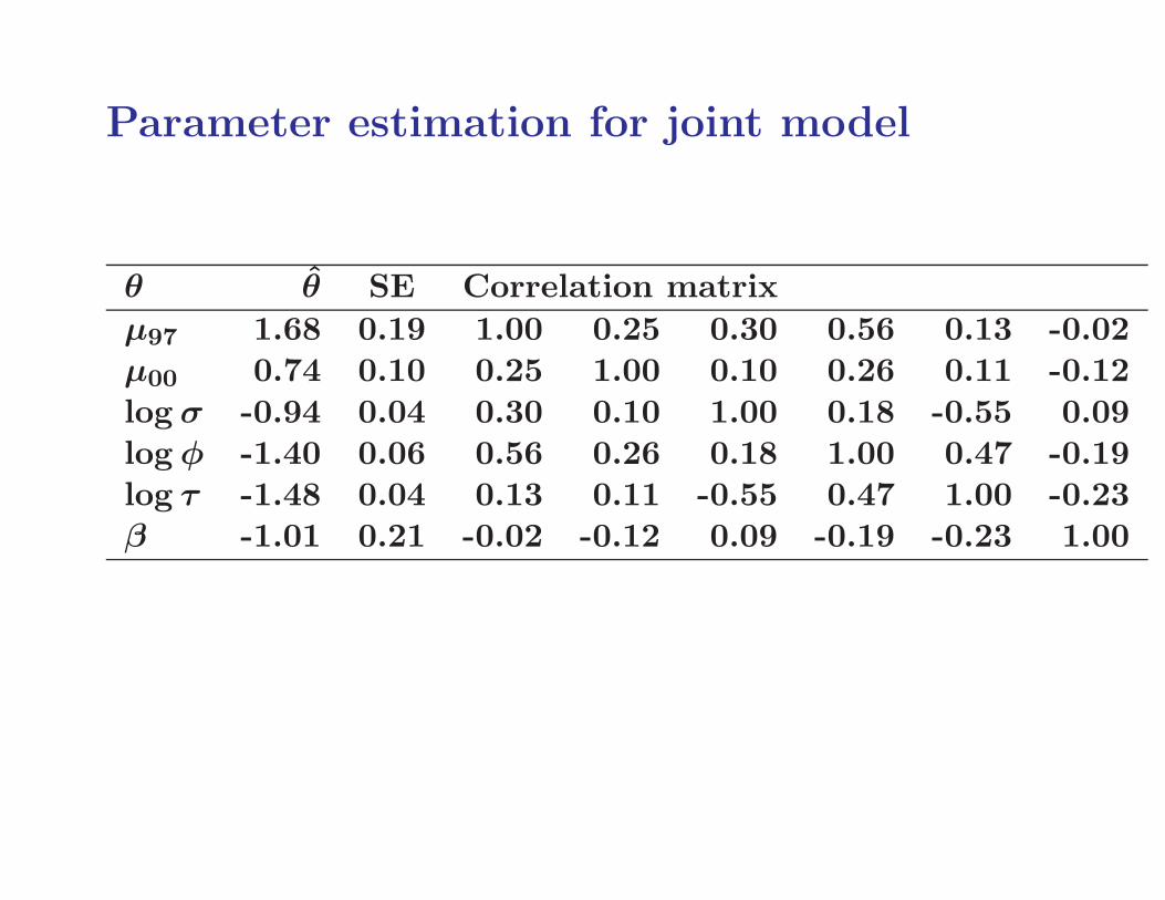
Parameter estimation for joint model
θ θ SE Correlation matrix
µ97 1.68 0.19 1.00 0.25 0.30 0.56 0.13 -0.02µ00 0.74 0.10 0.25 1.00 0.10 0.26 0.11 -0.12log σ -0.94 0.04 0.30 0.10 1.00 0.18 -0.55 0.09log φ -1.40 0.06 0.56 0.26 0.18 1.00 0.47 -0.19log τ -1.48 0.04 0.13 0.11 -0.55 0.47 1.00 -0.23β -1.01 0.21 -0.02 -0.12 0.09 -0.19 -0.23 1.00
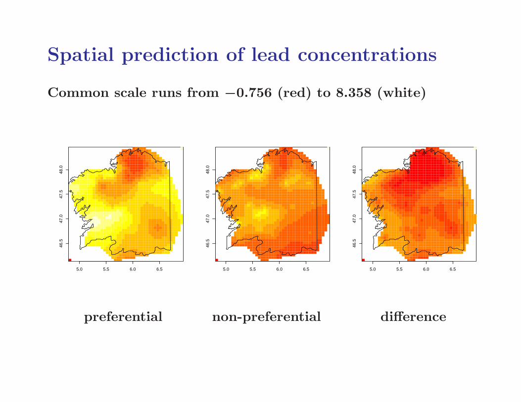
Spatial prediction of lead concentrations
Common scale runs from −0.756 (red) to 8.358 (white)
5.0 5.5 6.0 6.5
46.5
47.0
47.5
48.0
5.0 5.5 6.0 6.5
46.5
47.0
47.5
48.0
5.0 5.5 6.0 6.5
46.5
47.0
47.5
48.0
u)
preferential non-preferential difference
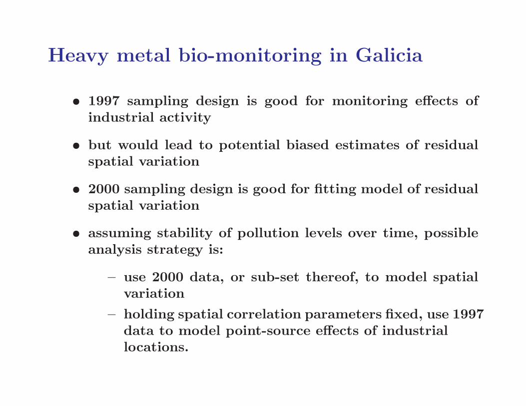
Heavy metal bio-monitoring in Galicia
• 1997 sampling design is good for monitoring effects ofindustrial activity
• but would lead to potential biased estimates of residualspatial variation
• 2000 sampling design is good for fitting model of residualspatial variation
• assuming stability of pollution levels over time, possibleanalysis strategy is:
– use 2000 data, or sub-set thereof, to model spatialvariation
– holding spatial correlation parameters fixed, use 1997data to model point-source effects of industriallocations.
Closing remarks
• There is nothing special about geostatistics.
• Parameter uncertainty can have a material impact onprediction.
• Bayesian paradigm deals naturally with parameteruncertainty.
• Implementation through MCMC is not whollysatisfactory:
– sensitivity to priors?
– convergence of algorithms?
– routine implementation on large data-sets?
• INLA shows great promise as alternative to MCMC
• Model-based approach clarifies distinctions between:
– the substantive problem;
– formulation of an appropriate model;
– inference within the chosen model;
– diagnostic checking and re-formulation.
• Analyse problems, not data:
– what is the scientific question?
– what data will best allow us to answer the question?
– what is a reasonable model to impose on the data?
– inference: avoid ad hoc methods if possible
– fit, reflect, re-formulate as necessary
– answer the question.
References
Crainiceanu, C., Diggle, P.J. and Rowlingson, B.S. (2008) Bivari-ate modelling and prediction of spatial variation in Loa loa preva-lence in tropical Africa (with Discussion). Journal of the American
Statistical Association, 103, 21–43.
Diggle, P.J. and Lophaven, S. (2006). Bayesian geostatistical de-sign. Scandinavian Journal of Statistics, 33, 55–64.
Diggle, P.J., Menezes, R. and Su, T.-L. (2010). Geostatistical anal-ysis under preferential sampling (with Discussion).Applied Statis-
tics, 59, 191–232.
Diggle, P.J., Moyeed, R.A. and Tawn, J.A. (1998). Model-basedGeostatistics (with Discussion). Applied Statistics 47 299–350.
Diggle, P.J. and Ribeiro, P.J. (2007). Model-based Geostatistics.New York: Springer.
Diggle, P.J., Thomson, M.C., Christensen, O.F., Rowlingson, B.,Obsomer, V., Gardon, J., Wanji, S., Takougang, I., Enyong, P.,Kamgno, J., Remme, H., Boussinesq, M. and Molyneux, D.H.(2007). Spatial modelling and prediction of Loa loa risk: deci-sion making under uncertainty. Annals of Tropical Medicine and
Parasitology, 101, 499–509.
Rue, H., Martino, S. and Chopin, N. (2009). Approximate Bayesianinference for latent Gaussian models by using integrated nestedLaplace approximations (with Discussion). Journal of the RoyalStatistical Society B 71, 319–392(see also http://www.r-inla.org/)