The slides are mainly from Silvio Savarese (U. of Michigan).

GEOMETRY and CALIBRATION

Lines in a 2D plane - Transformation

0cbyax

-c/b

slope -a/b

cba

l

If x = [ x1, x2]T line 0cba

1xx T

2

1

line

x

y point * line = 0

(new point) = H (old point) o.p. H H o.l. = 0(new line) = H (old line) H is 3x3 matrix

lines in projective transformation remain lines

T

-T

measured

T -TTransformation:

nonsingular in homogeneous coor.

T

Projective transformation of an ideal line (in 2D)

lHl T

bvtA

H

?lH T

btt

100

bvtA

y

xT

is it the line at infinity?

no, another line!

?lH TA

100

100

10

100

10 TT

TT

AtAtA

3x3

affine transformation

line atinfinity

T

T

nonsingular

Points and planes in 3D

1xxx

x3

2

1

dcba

0dczbyax

x

y

z

0xx T

Lines in 3D • Lines have 4 degrees of freedom. • Defined as intersection of 2 planes. (3 and 3 minus 2 the intersection line)

plane

Plane at infinity -- vanishing lines in 3D

1000

x

y

z

• Parallel planes in 3D intersect at the plane at infinity.

• Two planes are parallel iff their intersections is a line that belongs to

• Parallel planes intersect the plane at infinity in a common line – the vanishing line (horizon).

vanishing line a horizon

Parallel planes and at least two different parallel linefamily, defines a vanishing line which can be projected

on an image plane.

3D to 2D vanishing line

Projective transformation of l_inf in 2D

horizon

- Recognize the horizon line. - Measure if two lines meet at the horizon. - If yes, these two lines are parallel in 3D.

Are these two lines parallel or not?

lHl Thor

known

The image of 3D vanishing points

dv K

d=direction of the line d

C

v

In 3D a (homogeous) point on the line evolves P = [ P_0 + t * d 1 ]When t goes to infinity P_0 and 1, disappear. 3D ideal point P_inf = [ d 0]

3D nonhomogeneous vector

T

T

camera internal K [I 0] * P_inf

homogeous in 2Dideal point in the plane

(3x3)(3x1)

P_0

(time)

3D nonhomogeneous

P

3D nonhomogeneous

A line defined by 2 planes, not directly d.The 3D ideal point is along the line, that is d.

The image of 3D vanishing lines

C

n

Parallel planes intersect the plane at infinity in a common line – the vanishing line (horizon).

horizTK ln

horizl

Proof. d = K v is orthogonal to n d n = 0 v K n = 0 but v l_hor = 0

-1

T T -T

l_horiz (image) is obtained byintersecting a plane parallelwith the family through the camera center C.

3D nonhomogeneous normal

in the plane.

l_horiz 2D homogeneous

v

T

Vanishing points - example

C2

v2

C1

v1

R,T

11

11

1 KK

vvd

21

21

2 KK

vvd

21 R dd

v1, v2: measurement of vanishing points K = known and constant Can we compute R?

d_1,2 are directions of 3D parallel lines in image 1 and 2

translation does not play a role!

3D unit vectors

11

11

1 KK

vvd

21

21

2 KK

vvd

needs TWO corresponding directionsin each image - a vanishing line d(v1/2) and d(v3/4) 2x2 > 3

one corresponding direction

Five points define a conic in 2D

For each point the conic passes through

022 =+++++ feydxcyybxax iiiiii

or( ) 0,,,,, 22 =cfyxyyxx iiiiii ( )Tfedcba ,,,,,=c

0

11111

552555

25

442444

24

332333

23

222222

22

112111

21

=

⎥⎥⎥⎥⎥⎥

⎦

⎤

⎢⎢⎢⎢⎢⎢

⎣

⎡

c

yxyyxxyxyyxxyxyyxxyxyyxxyxyyxx

stacking constraints yields

determined upto a scale

- If a point x C

0feydxcybxyax 22

In homogeneous coordinates:

0xCxT

f2/e2/d2/ec2/b2/d2/ba

C

1xx

x 2

1

0xCxT

- If a line l is tangent to a conic in x xCl

1T PCPC - Projective transformation of conics:

P = H 3x3 nonsingular

for us here H is P

Proves for the conics:

The line l tangent to C at point x on C is given by l=Cx.

lx

C

x l = x C x = 0T T

Projective transformation of conicsx' = P x x C x = x' P C P x' = 0

T -T -1

C' = P C P-T -1

T

Circular points (see also lecture 2)

l

0i1

pi

0i1

p j

Circular points (point at infinity)

Circular points are fixed under similarity transformation.

0i1

0i1

100tcosssinstsinscoss

pH y

x

is

i2=-1 rotation around z axis

s e magnitude-i theta

plus translation

Conic C

Circular points define a degenerate

conic called ; any C

0x0xx

3

22

21

Cx

000010001

C0xCxT

l

0i1

pi

0i1

p j

Circular points (point at infinity)

is fixed under similarity transformation.

C

In 3D: absolute conic

Any x satisfies:

01

11

0xxT

0x0xxx

4

23

22

21

is fixed under 3D similarity transformation.

Do transformation from plane at infinity to camera plane.

P = K[R t]C' = (KR) I (KR) = K RR K = (K K )-T -1 -T -1 -1 T -1

is in 3D plane at infinity

2D projective transf. of the

It is not function of R, T

654

532

421

symmetric

02 zero-skew 31 square pixel

02

1.

2.

3. 4.

TRKP omega is in 2D theimage of the absolute conic (IAC)

(K K )T -1

also K K-T -1

Angle between two vanishing points

2T21

T1

2T1

vvvvvvcos

C

d1 v1

dv Kv2

d2

90 0vv 2T1

d = K v-1

cos(d , d )1 2

If between two raysin 3D

cos <d_1, d_2>

90

0vv 2T1

v1 v2

Constraint on K

(K K )T-1

Internal camera calibration...

zero-skewsquare pixels

...in a single view.

v2

v3

0vv 2T1

0vv 3T1

0vv 3T2

654

532

421

31

02

Compute :6 unknown - 1 scale5 constraints known up to scale

K (Cholesky factorization)

v2

(K K )T -1

R. Hartley and A. Zisserman: Multiple view geometry. Cambridge, 2004.

Cholesky factorization

A4.1 Orthogonal matrices 57 9

A4.1.1 Givens rotations and RQ decomposition

A 3-dimensional Given s rotation i s a rotation abou t one of the three coordinate axes . The three Givens rotations are

" 1 C s c —s c —s Qy = 1 Qz = s c s c —s c 1

where c = cos(6> ) and s = sin(0 ) fo r some angle 6 and blank entries represent zeros. Multiplying a 3 x 3 matrix A on the right by (for instance) Qz has the effect o f leaving

the last column o f A unchanged , an d replacing the first tw o columns by linear combi-nations of the original two columns. The angle 8 may be chosen so that any given entry in the first two columns becomes zero.

For instance, to set the entry A2i to zero, we need to solve the equation ca2i + sa<zi = 0. Th e solutio n t o this i s c = —022/(̂ 2 2 + a2iY^2 an< ^ s — a2i/(a|2 + a\\Y^• I t ' s

required tha t c 2 + ,s 2 = 1 since c = cos(# ) an d s — sin(0), and the values of c and s given here satisfy tha t requirement.

The strategy of the RQ algorithm is to clear out the lower half of the matrix one entry at a time by multiplication b y Givens rotations. Consider the decomposition o f a 3 x 3 matrix A a s A = R Q where R is upper-triangula r an d Q i s a rotation matrix . Thi s may take place in three steps . Eac h ste p consists of multiplication o n the right by a Givens rotation to set a chosen entry o f the matrix A to zero. Th e sequence of multiplications must be chosen in such a way as not to disturb the entries that have already been set to zero. An implementation o f the RQ decomposition is given in algorithm A4.1.

Objective

Carry out the RQ decomposition o f a 3 x 3 matrix A using Givens rotations.

Algorithm

(i) Multipl y by Qx so as to set A32 to zero, (ii) Multipl y by Qy so as to set A31 t o zero. This multiplication doe s not change the second

column of A, hence A 32 remains zero, (iii) Multipl y b y Qz so as t o se t A 2i t o zero . Th e first two columns ar e replaced b y linea r

combinations o f themselves. Thus , A31 and A32 remain zero.

Algorithm A4.1 . RQ decomposition of a 3 x3 matrix.

Other sequence s o f Given s rotation s ma y b e chose n t o giv e th e sam e result . A s a resul t o f thes e operations , w e fin d tha t AQ xQyQz = R where R is upper-triangular . Consequently, A = RQjQ^Qj , an d s o A = R Q where Q = QjQj[Q j i s a rotation. I n addition, the angles 6X, 0y an d 9Z associated with the three Givens rotations provide a parametrization o f th e rotation b y thre e Eule r angles , otherwis e know n a s roll , pitc h and yaw angles.

It should be clear from thi s description o f the decomposition algorith m how simila r QR, QL and LQ factorizations may be carried out. Furthermore, the algorithm is easily generalized to higher dimensions.

a_31 and a_33 change

a_21 and a_22 change

a_32 and a_33 changein the lower-triangular part:

No distortion

Pin cushion

Barrel

Radial Distortion – Caused by imperfect lenses. – Deviations are most noticeable for rays that pass through

the edge of the lens.

Radial distortion included in the 2D calibration.

ii

ii p

vu

PM

100

00

00

1

1

d

v

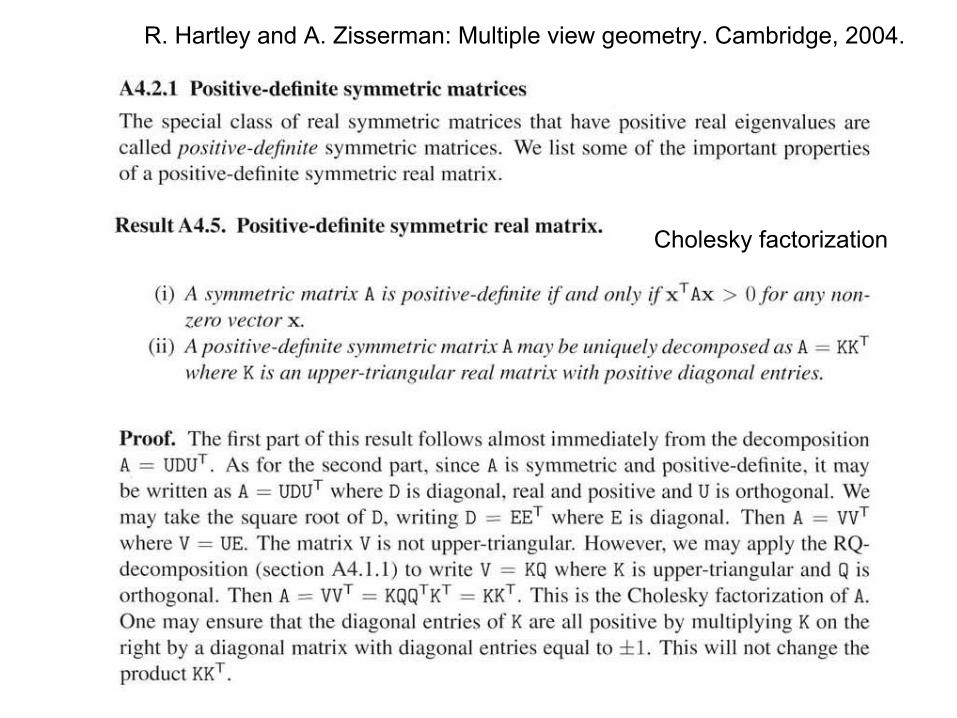
vucvbuad 222

u

3

1p

2ppdκ1λ

polynomial function

distortion coefficient

To model radial behavior in general d = u + v 2 2 2

the image coor. u,v, are distorted

2

Radial Distortion

i

ii v

up

i3

i2

i3

i1

PPPP

1

mmmm

m

We find the (two) coefficients (r and r ) by requesting that straight lines should be straight.

2 4

T

T

T

T

nonlinear function

before radial distortion was removed

after radial distortion was removed

Correcting Radial Lens Distortions

Before After

http://www.grasshopperonline.com/barrel_distortion_correction_software.html

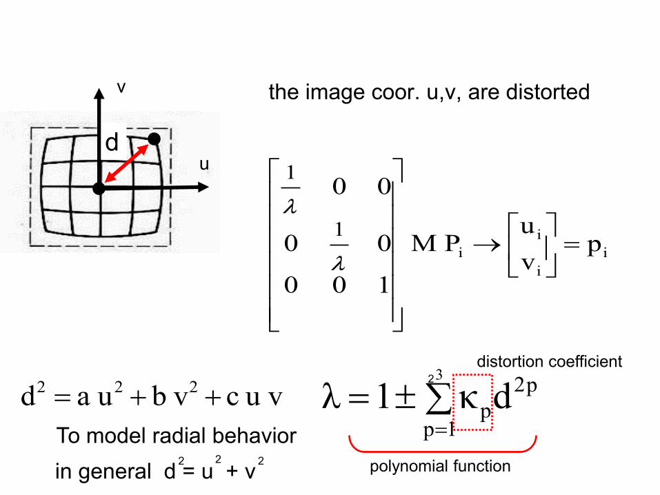
Calibration Procedure Camera Calibration Toolbox for Matlab J. Bouguet – [1998-2000] http://www.vision.caltech.edu/bouguetj/calib_doc/index.html#examples

see webpage

with aplane

Take images of a planar checkerboard.

For each image click in this order on the four extreme corners.

The image corners are then automatically extracted.

After the estimation was done, we have 11 parameters (max.) (12 parameters divided by the scale)

The first three columns of the recovered matrix give the 5 intrinsic parameters through image of the absolute conic which we saw before => K (some given!)

For rotation have to add orthonormality of the three directionsand R ~ K M_13. Translation is obtained t = K m_4.

There are 6 extrinsic parameters. All X_i’s in 3D cannot lie on the same plane.

-1 -1

[M_13 m_4] or K [R t]

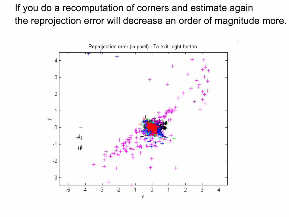
If you do a recomputation of corners and estimate againthe reprojection error will decrease an order of magnitude more.

camera viewpoint

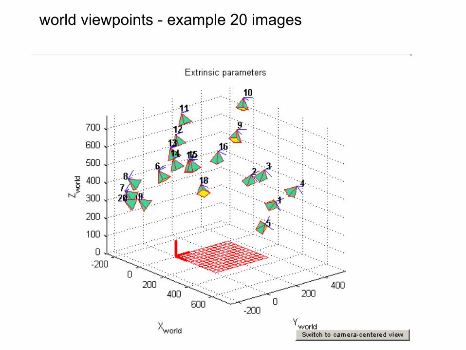
world viewpoints - example 20 images

Calibration problem directly 3D to 2D

•P1… Pn with known positions in [Ow,iw,jw,kw] P=X•p1, … pn known positions in the image p=x Goal: compute intrinsic and extrinsic parameters

jC

Calibration rig

Linear method 3D to 2D

ii PXx =λ 0PXx =× ii0XP

XP

2

1

=⎥⎥⎥⎤

⎢⎢⎢⎡

×⎥⎥⎤

⎢⎢⎡

iT

iT

i

i

yx

ii iiXP1 3⎥⎦⎢⎣⎥

⎥⎦⎢

⎢⎣ i

T

PXX0 ⎞⎛⎤⎡ TT

0PP

X0XXX0

2

1

=⎟⎟⎟⎞

⎜⎜⎜⎛

⎥⎥⎥⎤

⎢⎢⎢⎡

−−

Tii

Ti

Tii

Ti

xy

P0XX 3⎟⎠

⎜⎝⎥⎦⎢⎣−

Tii

Tii xy

Two linearly independent equations.

homogeneous coordinates

P a 3x4 matrix -- will need 6 correspondences.

image jC

Calibration rig

In practice: user may need to look at the image and select the n > 6 correspondences. Today used only if very precise calibration is needed.

After the camera was calibrated...

TRKM

C

Ow

If K, R, T are known – the center C is also defined. Can we estimate P from p based on a single image?

P p

NO - since P can be anywhere along the line defined by C and p.