Embed Size (px)
Citation preview

Gaussian Channels: Information, Estimation and
Multiuser Detection
Dongning Guo
A Dissertation
Presented to the Faculty
of Princeton University
in Candidacy for the Degree
of Doctor of Philosophy
Recommended for Acceptance
by the Department of
Electrical Engineering
November, 2004

c© Copyright by Dongning Guo, 2004.
All rights reserved.

Abstract
This thesis represents an addition to the theory of information transmission, signal estima-tion, nonlinear filtering, and multiuser detection over channels with Gaussian noise. Thework consists of two parts based on two problem settings—single-user and multiuser—whichdraw different techniques in their development.
The first part considers canonical Gaussian channels with an input of arbitrary but fixeddistribution. An “incremental channel” is devised to study the mutual information increasedue to an infinitesimal increase in the signal-to-noise ratio (SNR) or observation time. Itis shown that the derivative of the input-output mutual information (nats) with respectto the SNR is equal to half the minimum mean-square error (MMSE) achieved by optimalestimation of the input given the output. This relationship holds for both scalar and vectorsignals, as well as for discrete- and continuous-time models. This information-theoreticresult has an unexpected consequence in continuous-time estimation: The causal filteringMMSE achieved at SNR is equal to the average value of the noncausal smoothing MMSEachieved with a channel whose signal-to-noise ratio is chosen uniformly distributed between0 and SNR.
The second part considers Gaussian multiple-access channels, in particular code-divisionmultiple access (CDMA), where the input is the superposition of signals from many users,each modulating independent symbols of an arbitrary distribution onto a random signaturewaveform. The receiver conducts optimal joint decoding or suboptimal separate decod-ing that follows a posterior mean estimator front end, which can be particularized to thematched filter, decorrelator, linear MMSE detector, and the optimal detectors. Large-system performance of multiuser detection is analyzed in a unified framework using thereplica method developed in statistical physics. It is shown under replica symmetry as-sumption that the posterior mean estimate, which is generally non-Gaussian in distribu-tion, converges to a deterministic function of a hidden Gaussian statistic. Consequently, themultiuser channel can be decoupled into equivalent single-user Gaussian channels, wherethe degradation in SNR due to multiple-access interference, called multiuser efficiency, isdetermined by a fixed-point equation. The multiuser efficiency uniquely characterizes theerror performance and input-output mutual information of each user, as well as the overallsystem spectral efficiency.
iii


Acknowledgements
I am indebted to my advisor, Professor Sergio Verdu, for his support, encouragement, andinvaluable advice during the course of my Ph.D. study. Sergio has set an example of a greatscholar that would be my goal for many years to come.
I am very grateful to my collaborator, Dr. Shlomo Shamai, whose ideas, suggestions andenormous knowledge of the research literature have benefited me a lot.
I would like to thank Shlomo, Dr. H. Vincent Poor, Dr. Robert Calderbank and Dr.Mung Chiang for serving in my thesis committee.
Thanks to Chih-Chun for many discussions, to Juhua for always sharing her wisdom,and all my friends both at Princeton and elsewhere who made the last five years full of fun.
This thesis is dedicated to my parents and grandparents.
v


Contents
Abstract iii
Acknowledgements v
Contents vii
List of Figures ix
1 Introduction 11.1 Mutual Information and MMSE . . . . . . . . . . . . . . . . . . . . . . . . . 11.2 Multiuser Channels . . . . . . . . . . . . . . . . . . . . . . . . . . . . . . . . 21.3 Notation . . . . . . . . . . . . . . . . . . . . . . . . . . . . . . . . . . . . . . 4
2 Mutual Information and MMSE 52.1 Introduction . . . . . . . . . . . . . . . . . . . . . . . . . . . . . . . . . . . . 52.2 Scalar and Vector Channels . . . . . . . . . . . . . . . . . . . . . . . . . . . 7
2.2.1 The Scalar Gaussian-noise Channel . . . . . . . . . . . . . . . . . . . 72.2.2 A Vector Channel . . . . . . . . . . . . . . . . . . . . . . . . . . . . 92.2.3 Proof via the SNR-Incremental Channel . . . . . . . . . . . . . . . . 102.2.4 Discussions . . . . . . . . . . . . . . . . . . . . . . . . . . . . . . . . 132.2.5 Some Applications of Theorems 2.1 and 2.2 . . . . . . . . . . . . . . 162.2.6 Alternative Proofs of Theorems 2.1 and 2.2 . . . . . . . . . . . . . . 172.2.7 Asymptotics of Mutual Information and MMSE . . . . . . . . . . . . 19
2.3 Continuous-time Channels . . . . . . . . . . . . . . . . . . . . . . . . . . . . 212.3.1 Mutual Information Rate and MMSEs . . . . . . . . . . . . . . . . . 232.3.2 The SNR-Incremental Channel . . . . . . . . . . . . . . . . . . . . . 272.3.3 The Time-Incremental Channel . . . . . . . . . . . . . . . . . . . . . 28
2.4 Discrete-time vs. Continuous-time . . . . . . . . . . . . . . . . . . . . . . . 292.4.1 A Fourth Proof of Theorem 2.1 . . . . . . . . . . . . . . . . . . . . . 302.4.2 Discrete-time Channels . . . . . . . . . . . . . . . . . . . . . . . . . 31
2.5 Generalizations and Observations . . . . . . . . . . . . . . . . . . . . . . . . 322.5.1 General Additive-noise Channel . . . . . . . . . . . . . . . . . . . . . 322.5.2 New Representation of Information Measures . . . . . . . . . . . . . 342.5.3 Generalization to Vector Models . . . . . . . . . . . . . . . . . . . . 35
2.6 Summary . . . . . . . . . . . . . . . . . . . . . . . . . . . . . . . . . . . . . 36
vii

3 Multiuser Channels 373.1 Introduction . . . . . . . . . . . . . . . . . . . . . . . . . . . . . . . . . . . . 37
3.1.1 Gaussian or Non-Gaussian? . . . . . . . . . . . . . . . . . . . . . . . 373.1.2 Random Matrix vs. Spin Glass . . . . . . . . . . . . . . . . . . . . . 40
3.2 Model and Summary of Results . . . . . . . . . . . . . . . . . . . . . . . . . 423.2.1 System Model . . . . . . . . . . . . . . . . . . . . . . . . . . . . . . . 423.2.2 Posterior Mean Estimation . . . . . . . . . . . . . . . . . . . . . . . 433.2.3 Specific Detectors . . . . . . . . . . . . . . . . . . . . . . . . . . . . 453.2.4 Main Results . . . . . . . . . . . . . . . . . . . . . . . . . . . . . . . 463.2.5 Recovering Known Results . . . . . . . . . . . . . . . . . . . . . . . 523.2.6 Discussions . . . . . . . . . . . . . . . . . . . . . . . . . . . . . . . . 55
3.3 Multiuser Communications and Statistical Physics . . . . . . . . . . . . . . 573.3.1 A Note on Statistical Physics . . . . . . . . . . . . . . . . . . . . . . 573.3.2 Communications and Spin Glasses . . . . . . . . . . . . . . . . . . . 583.3.3 Free Energy and Self-averaging Property . . . . . . . . . . . . . . . . 603.3.4 Spectral Efficiency of Jointly Optimal Decoding . . . . . . . . . . . . 613.3.5 Separate Decoding . . . . . . . . . . . . . . . . . . . . . . . . . . . . 613.3.6 Replica Method . . . . . . . . . . . . . . . . . . . . . . . . . . . . . . 62
3.4 Proofs Using the Replica Method . . . . . . . . . . . . . . . . . . . . . . . . 643.4.1 Free Energy . . . . . . . . . . . . . . . . . . . . . . . . . . . . . . . . 643.4.2 Joint Moments . . . . . . . . . . . . . . . . . . . . . . . . . . . . . . 71
3.5 Complex-valued Channels . . . . . . . . . . . . . . . . . . . . . . . . . . . . 763.6 Numerical Results . . . . . . . . . . . . . . . . . . . . . . . . . . . . . . . . 783.7 Summary . . . . . . . . . . . . . . . . . . . . . . . . . . . . . . . . . . . . . 87
4 Conclusion and Future Work 89
A 91A.1 A Fifth Proof of Theorem 2.1 . . . . . . . . . . . . . . . . . . . . . . . . . . 91A.2 A Fifth Proof of Theorem 2.2 . . . . . . . . . . . . . . . . . . . . . . . . . . 92A.3 Proof of Lemma 2.5 . . . . . . . . . . . . . . . . . . . . . . . . . . . . . . . 95A.4 Asymptotic Joint Normality of {V } . . . . . . . . . . . . . . . . . . . . . . 97A.5 Evaluation of G(u) . . . . . . . . . . . . . . . . . . . . . . . . . . . . . . . . 98A.6 Proof of Lemma 3.2 . . . . . . . . . . . . . . . . . . . . . . . . . . . . . . . 99A.7 Proof of Lemma 2.6 . . . . . . . . . . . . . . . . . . . . . . . . . . . . . . . 100
References 101
Index 109
viii

List of Figures
2.1 The mutual information (in nats) and MMSE of a scalar Gaussian channelwith Gaussian and binary inputs, respectively. . . . . . . . . . . . . . . . . 9
2.2 An SNR-incremental Gaussian channel. . . . . . . . . . . . . . . . . . . . . 122.3 A Gaussian pipe where noise is added gradually. . . . . . . . . . . . . . . . 142.4 Sample paths of the input and output processes of an additive white Gaussian
noise channel, the output of the optimal forward and backward filters, as wellas the output of the optimal smoother. The input {Xt} is a random telegraphwaveform with unit transition rate. The SNR is 15 dB. . . . . . . . . . . . . 22
2.5 The causal and noncausal MMSEs of continuous-time Gaussian channel witha random telegraph waveform input. The transition rate ν = 1. The twoshaded regions have the same area due to Theorem 2.8. . . . . . . . . . . . 26
2.6 A continuous-time SNR-incremental Gaussian channel. . . . . . . . . . . . . 272.7 A general additive-noise channel. . . . . . . . . . . . . . . . . . . . . . . . . 33
3.1 The probability density function obtained from the histogram of an individu-ally optimal soft detection output conditioned on +1 being transmitted. Thesystem has 8 users, the spreading factor is 12, and the SNR 2 dB. . . . . . . 39
3.2 The probability density function obtained from the histogram of the hiddenequivalent Gaussian statistic conditioned on +1 being transmitted. The sys-tem has 8 users, the spreading factor is 12, and the SNR 2 dB. The asymptoticGaussian distribution is also plotted for comparison. . . . . . . . . . . . . . 39
3.3 The CDMA channel with joint decoding. . . . . . . . . . . . . . . . . . . . . 423.4 The CDMA channel with separate decoding. . . . . . . . . . . . . . . . . . 433.5 The equivalent scalar Gaussian channel followed by a decision function. . . 473.6 The equivalent single-user Gaussian channel, posterior mean estimator and
retrochannel. . . . . . . . . . . . . . . . . . . . . . . . . . . . . . . . . . . . 513.7 A canonical interference canceler equivalent to the single-user Gaussian channel. 563.8 A canonical channel, its corresponding retrochannel, and the generalized PME. 583.9 The replicas of the retrochannel. . . . . . . . . . . . . . . . . . . . . . . . . 623.10 Simulated probability density function of the posterior mean estimates under
binary input conditioned on “+1” being transmitted. Systems with 4, 8, 12and 16 equal-power users are simulated with β = 2/3. The SNR is 2 dB. . . 79
3.11 Simulated probability density function of the “hidden” Gaussian statisticrecovered from the posterior mean estimates under binary input conditionedon “+1” being transmitted. Systems with 4, 8, 12 and 16 equal-power usersare simulated with β = 2/3. The SNR is 2 dB. The asymptotic Gaussiandistribution predicted by our theory is also plotted for comparison. . . . . . 79
3.12 The multiuser efficiency vs. average SNR (Gaussian inputs, β = 1). . . . . . 81
ix

3.13 The spectral efficiency vs. average SNR (Gaussian inputs, β = 1). . . . . . . 813.14 The multiuser efficiency vs. average SNR (binary inputs, β = 1). . . . . . . 823.15 The spectral efficiency vs. average SNR (binary inputs, β = 1). . . . . . . . 823.16 The multiuser efficiency vs. average SNR (8PSK inputs, β = 1). . . . . . . . 833.17 The spectral efficiency vs. average SNR (8PSK inputs, β = 1). . . . . . . . . 833.18 The multiuser efficiency vs. average SNR (Gaussian inputs, β = 3). . . . . . 843.19 The spectral efficiency vs. average SNR (Gaussian inputs, β = 3). . . . . . . 843.20 The multiuser efficiency vs. average SNR (binary inputs, β = 3). . . . . . . 853.21 The spectral efficiency vs. average SNR (binary inputs, β = 3). . . . . . . . 853.22 The multiuser efficiency vs. average SNR (8PSK inputs, β = 3). . . . . . . . 863.23 The spectral efficiency vs. average SNR (8PSK inputs, β = 3). . . . . . . . . 86
x

Chapter 1
Introduction
The exciting revolution in communication technology in recent years would not have beenpossible without significant advances in detection, estimation, and information theory sincethe mid-twentieth century. This thesis represents an addition to the theory of informationtransmission, signal estimation, nonlinear filtering and multiuser detection over channelswith Gaussian noise.
“The fundamental problem of communication,” described by Shannon in his 1948 land-mark paper [86], “is that of reproducing at one point either exactly or approximately amessage selected at another point.” Typically, communication engineers are given a phys-ical channel, which, upon an input signal representing the message, generates an outputsignal coupled with the input. The problem is then to determine which message was sentamong all possibilities based on the observed output and knowledge about the channel.
A key index of success is how many distinct messages, or in more abstract sense, theamount of information that can be communicated reliably through the channel. This ismeasured by the notion of mutual information. Meanwhile, the difficulty faced by com-munication engineers is how much error the receiver would make in estimating the inputsignal given the output. A key measure here is the minimum mean-square error (MMSE)due to its tractability and practical effectiveness. This thesis is centered around the input-output mutual information and MMSE of Gaussian channels, whose output is equal to theinput plus random noise of Gaussian distribution. Two problem settings—single-user andmultiuser—which draw different techniques in their development, consist of the two mainchapters (Chapters 2 and 3) of the thesis.
1.1 Mutual Information and MMSE
Chapter 2 deals with the transmission of an arbitrarily distributed input signal from a singlesource (user). Since Wiener’s pioneer work in 1940s [114], a rich theory of detection andestimation in Gaussian channels has been developed [59], notably the matched filter [74], theRAKE receiver [79], the likelihood ratio (e.g., [78]), and the estimator-correlator principle(e.g., [92, 84, 56]). Alongside was the development of the theory of stochastic processesand stochastic calculus since 1930s that set the mathematical stage. Shannon, the founderof information theory, obtained the capacity of Gaussian channels under power constraint[86]. Since then, much has been known about the information theory of Gaussian channels,as well as practical codes that achieve rates very close to the channel capacity.
Information theory and the theory of detection and estimation have largely been treated
1

2 Introduction
separately, although numerous results and techniques connect the two. In the Gaussianregime, information and estimation have strong ties through known likelihood ratios. Forexample, by taking the expectation of the “estimator-correlator” type of log-likelihood ratiosin continuous-time problems, Duncan found that the input-output mutual information canbe expressed as a time-average of the MMSE of causal filtering [21].
Encompassing not only continuous-time, but also discrete-time channels, as well asscalar random transformations with additive Gaussian noise, Chapter 2 finds a fundamentalrelationship between the input-output mutual information and MMSE, which is unknownuntil this work. That is, the derivative of the mutual information (nats) with respect to thesignal-to-noise ratio (SNR) is equal to half the MMSE, achieved by (noncausal) conditionalmean estimation. The relationships holds for vector as well as scalar inputs of arbitrary butfixed distribution. Using these information-theoretic results, a new relationship is foundin continuous-time nonlinear filtering: Regardless of the input signal statistics, the causalfiltering MMSE achieved at SNR is equal to the expected value of the noncausal smoothingMMSE achieved with a channel whose signal-to-noise ratio is chosen uniformly distributedbetween 0 and SNR.
The connection between information and estimation is drawn through a key observationthat the mutual information of a small SNR Gaussian channel is essentially the input vari-ance times the SNR. This is due to the geometry of the likelihood ratio associated with theGaussian channel. Major results in Chapter 2 are proved by using the idea of “incrementalchannels” to investigate the increase of mutual information due to an infinitesimal increasein SNR or observation time.
In a nutshell, Chapter 2 reveals a “hidden” link between information and estimationtheory. The new relationship facilitates interactions of the two fields and lead to interestingresults.
1.2 Multiuser Channels
Chapter 3 studies multiuser communication systems where individual user’s mutual in-formation and estimation error are of interest. Each user modulates coded symbols ontoa multidimensional signature waveform which is randomly generated. The input to theGaussian channel is the superposition of signals from many users, where the users are dis-tinguished by their signature waveforms. This model is often referred to as code-divisionmultiple access (CDMA), but is also a popular paradigm of many multi-input multi-output(MIMO) channels. The most efficient use of such a channel is by optimal joint decoding,the complexity of which is rarely affordable in practice. A common suboptimal strategy isto apply a multiuser detector front end which generates an estimate of the input symbolsof each user and then perform independent single-user decoding.
Detection and estimation of multiuser signals are well studied [112]. It is often impossi-ble to maintain orthogonality of the signatures and hence interference among users degradesperformance. Various interference suppression techniques provide a wide spectrum of trade-offs between performance and complexity. Detectors range from the primitive single-usermatched filter, to the decorrelator, linear MMSE detector, sophisticated interference can-celers, and the jointly and individually optimal detectors. Performance analysis of variousmultiuser detection techniques is of great theoretical and practical interest.
Verdu first used the concept of multiuser efficiency to refer to the SNR degradationrelative to a single-user channel calibrated at the same bit-error-rate (BER) [107]. Exact

1.2 Multiuser Channels 3
evaluation of the multiuser efficiency of even the simplest matched filter can be highly com-plex, since the multiple access interference (MAI), which shows up in detection outputs,often takes an exponential number of different values. More recently, much attention isdevoted to the large-system regime, where dependence of performance on signature wave-forms diminishes. For most linear front ends of interest, regardless of the input, the MAI indetection output is asymptotically normal, which is tantamount to an enhancement of thebackground Gaussian noise. Thus the multiuser channel can be decoupled into single-userones with a degradation in the effective SNR. As far as linear detectors are concerned, themultiuser efficiency directly maps to the SNR of detection output, which completely charac-terizes large-system performance, and can often be obtained analytically, e.g., [112, 99, 44].Unfortunately, the traditional wisdom of asymptotic normality fails in case of nonlineardetectors, since the detection output is in general non-Gaussian in the large-system limit.Analytical result for performance is scarce and numerical analysis is costly but often theonly resort.
Chapter 3 unravels several outstanding problems in multiuser detection and its informa-tion theory. A family of multiuser detectors is analyzed in a unified framework by treatingeach detector as a posterior mean estimator (PME) informed with a carefully chosen pos-terior probability distribution. Examples of such detectors include the above-mentionedlinear detectors, as well as the optimal nonlinear detectors. One of the key results is thatthe detection output of all such detectors, although asymptotically non-Gaussian in general,converges to a deterministic function of a “hidden” Gaussian statistic centered at the trans-mitted symbol. Hence asymptotic normality is still valid subject to an inverse function, andsystem performance can nonetheless be fully characterized by a scalar parameter, the mul-tiuser efficiency, which is found to satisfy a fixed-point equation along with the MMSE of anadjunct Gaussian channel. Moreover, the spectral efficiencies, i.e., total mutual informationper dimension, under both joint and separate decoding are found in simple expressions inthe multiuser efficiency.
The methodology applied in Chapter 3 is rather unconventional. The many-user com-munication system is regarded as a thermodynamic system consisting of a large numberof interacting particles, known as a spin glass. The system is studied in the large-systemlimit using the replica method developed in statistical physics. We leave the “self-averagingproperty”, the “replica trick” and replica symmetry assumption unjustified, which are them-selves notoriously difficult challenges in mathematical physics. The general results obtainedare consistent with known results in special cases, and supported by numerical example.
The use of the replica method in multiuser detection was introduced by Tanaka [96],who also suggested special-case PME with postulated posteriors, although referred to as themarginal-posterior-mode detectors. Chapter 3 puts forth the “decoupling principle” therebyenriching Tanaka’s groundbreaking framework. The replica analysis is also developed in thischapter to a full generality in signaling and detection schemes based on [96].
In all, this thesis studies mutual information, posterior mean estimation and their inter-actions, and presents single-user and multiuser variations on this theme. In the single-usersetting (Chapter 2), a fundamental formula that links mutual information and MMSE isdiscovered, which points to new relationships, applications, and open problems. In the mul-tiuser setting (Chapter 3), the multidimensional channel with a rich structure is essentiallydecoupled into equivalent single-user Gaussian channels where the SNR degradation is fully

4 Introduction
quantified.1 In either case, the results speak of new connections between the fundamentallimits of digital communications to those of analog signal processing.
1.3 Notation
Throughout this thesis, random objects and matrices are denoted by upper case lettersunless otherwise noted. Vectors and matrices are in bold font. For example, x denotesa number, x a column vector, X a scalar random variable, X a random column vector,S a matrix which is either random or deterministic depending on the context. Gaussiandistribution with mean m and variance σ2 is denoted by N
(m,σ2
)and unit Gaussian
random noise is usually denoted by the letter N . In general, PX denotes the probabilitymeasure (or distribution) of the random object X. The probability density function, ifexists, is denoted by pX . Sometimes qX also denotes a probability density function todistinguish from pX . An expectation E {·} is taken over the joint distribution of the randomvariables within the braces. Conditional expectation is denoted by E {· | ·}. In general,notations are introduced at first occurrence.
1Chronologically most of the results in Chapter 3 were obtained before those in Chapter 2. In fact, it wasthe process of proving Theorem 3.1 that prompted Theorem 2.1 and thereby the main theme of Chapter 2.After reading an earlier version of [43] Professor Shlomo Shamai came up independently of us with a proofof Theorem 2.1 using Duncan’s Theorem (see Section 2.4.1). Upon finding out that we had obtained similarresults independently we joined forces, and the results in Chapter 2 have been obtained in close cooperationwith both my thesis advisor, Professor Sergio Verdu and Professor Shlomo Shamai.

Chapter 2
Mutual Information and MMSE
This chapter unveils several new relationships between the input-output mutual informationand MMSE of Gaussian channels. The relationships are shown to hold for arbitrarilydistributed input signals and the broadest settings of Gaussian channels. Although thesignaling can be multidimensional, the input is regarded as a whole from a single source.Multiuser problems where individual user’s performance is of interest will be studied inChapter 3.
2.1 Introduction
Consider an arbitrary pair of jointly distributed random objects (X, Y ). The mutual in-formation, which stands for the amount of information contained in one of them about theother, is defined as the expectation of the logarithm of the likelihood ratio (Radon-Nikodymderivative) between the joint probability measure and the product of the marginal measures[60, 75]:
I(X;Y ) =∫
logdPXY
dPX dPYdPXY . (2.1)
Oftentimes, one would also want to infer the value of X from Y . An estimate of X givenY is essentially a function of Y , which is desired to be close to X in some sense. Supposethat X resides in a metric space with L2-norm defined, then the mean-square error of anestimate f(Y ) of X is given by
msef (X|Y ) = E{|X − f(Y )|2
}, (2.2)
where the expectation is taken over the joint distribution PXY . It is well-known that theminimum of (2.2), referred to as the minimum mean-square error or MMSE, is achieved byconditional mean estimation (CME) (e.g., [76]):
X(Y ) = E {X | Y } , (2.3)
where the expectation is over the posterior probability distribution PX|Y . In Bayesian statis-tics literature, the CME is also known as the posterior mean estimation (PME). Clearly,both mutual information and MMSE are measures of dependence between two randomobjects.
In general, (X, Y ) can be regarded as the input-output pair of a channel characterizedby the random transformation PY |X and input distribution PX . The mutual information
5

6 Mutual Information and MMSE
is then a measure of how many distinct input sequences are distinguishable on averageby observing the output sequence from repeated and independent use of such a channel.Meanwhile, the MMSE stands for the minimum error in estimating each input X using theobservation Y while being informed of the posterior distribution PX|Y .
This thesis studies the important case where X and Y denote the input and outputof an additive Gaussian noise channel respectively. Take for example the simplest scalarGaussian channel with an arbitrary input. Fix the input distribution. Let the powerratio of the signal and noise components seen in the channel output, i.e., signal-to-noiseratio, be denoted by snr. Both the input-output mutual information and the MMSE arethen monotonic functions of the SNR, denoted by I(snr) and mmse(snr) respectively. Thischapter finds that the mutual information in nats and the MMSE satisfy the followingrelationship regardless of the input statistics:
ddsnr
I(snr) =12mmse(snr). (2.4)
Simple as it is, the identity (2.4) was unknown before this work. It is trivial that one cango from one monotonic function to another by simply composing the inverse function of onewith the other; what is quite surprising here is that the overall transformation is not onlystrikingly simple but also independent of the input distribution. In fact the relationship(2.4) and its variations hold under arbitrary input signaling and the broadest settings ofGaussian channels, including discrete-time and continuous-time channels, either in scalaror vector versions.
In a wider context, the mutual information and mean-square error are at the core ofinformation theory and signal processing respectively. Thus not only is the significance ofa formula like (2.4) self-evident, but the relationship is intriguing and deserves thoroughexposition.
At zero SNR, the right hand side of (2.4) is equal to one half of the input variance.In that special case the identity, and in particular, the fact that at low SNRs the mutualinformation is insensitive to the input distribution has been remarked before [111, 61, 104].Relationships between the local behavior of mutual information at vanishing SNR and theMMSE are given in [77].
Formula (2.4) can be proved using a new idea of “incremental channels”, which is toanalyze the increase in the mutual information due to an infinitesimal increase in SNR,or equivalently, the decrease in mutual information due to an independent extra Gaussiannoise which is infinitesimally small. The change in mutual information is found to be equalto the mutual information of a Gaussian channel whose SNR is infinitesimally small, inwhich region the mutual information is essentially linear in the estimation error, and hencerelates the rate of mutual information increase to the MMSE.
A deeper reasoning of the relationship, however, traces to the geometry of Gaussianchannels, or, more tangibly, the geometric properties of the likelihood ratio associated withsignal detection in Gaussian noise. Basic information-theoretic notions are firmly associatedwith the likelihood ratio, and foremost is the mutual information. The likelihood ratio alsoplays a fundamental role in detection and estimation, e.g., in hypothesis testing, it is com-pared to a threshold to determine which hypothesis to take. Moreover, the likelihood ratiois central in the connection of detection and estimation, in either continuous-time setting[55, 56, 57] or discrete one [48]. In fact, Esposito [27] and Hatsell and Nolte [46] notedsimple relationships between conditional mean estimation and the gradient and Laplacianof the log-likelihood ratio respectively, although they did not import mutual information

2.2 Scalar and Vector Channels 7
into the picture. Indeed, the likelihood ratio bridges information measures and basic quan-tities in detection and estimation, and in particular, the estimation errors (e.g., [65]). Therelationships between information and estimation have been continuously used to evaluateresults in one area taking advantage of known results from the other. This is best exempli-fied by the classical capacity-rate distortion relations, that have been used to develop lowerbounds on estimation errors on one hand [119] and on the other to find achievable boundsfor mutual information based on estimation errors associated with linear estimators [31].
The central formula (2.4) holds in case of continuous-time Gaussian channels as well,where the left hand side shall be replaced by the input-output mutual information rate,and the right hand side by the average noncausal smoothing MMSE per unit time. Theinformation-theoretic result has also a surprising consequence in relating the causal andnoncausal MMSEs, which becomes clear in Section 2.3.
In fact, the relationship between the mutual information and noncausal estimation errorholds in even more general settings of Gaussian channels. Zakai has recently generalizedthe central formula (2.4) to the abstract Wiener space [120].
The remainder of this chapter is organized as follows. Section 2.2 deals with randomvariable/vector channels, while continuous-time channels are considered in Section 2.3. In-teractions between discrete- and continuous-time models are studied in Section 2.4. Resultsfor general channels and information measures are presented in Section 2.5.
2.2 Scalar and Vector Channels
2.2.1 The Scalar Gaussian-noise Channel
Consider a real-valued scalar Gaussian-noise channel of the canonical form:
Y =√
snr X + N, (2.5)
where snr denotes the signal-to-noise ratio of the observed signal,1 and the noise N ∼N (0, 1) is a standard Gaussian random variable independent of the input, X. The input-output conditional probability density is described by
pY |X;snr(y|x; snr) =1√2π
exp[−1
2(y −
√snr x
)2]. (2.6)
Let the distribution of the input be PX , which does not depend on snr. The marginalprobability density function of the output exists:
pY ;snr(y; snr) = E{pY |X;snr(y|X; snr)
}, ∀y. (2.7)
Given the channel output, the MMSE in estimating the input is a function of snr:
mmse(snr) = mmse(X |
√snr X + N
). (2.8)
The input-output mutual information of the channel (2.5) is also a function of snr. Let itbe denoted by
I(snr) = I(X;√
snr X + N). (2.9)
1If EX2 = 1 then snr complies with the usual notion of signal-to-noise power ratio Es/σ2.

8 Mutual Information and MMSE
To start with, consider the special case when the distribution PX of the input X isstandard Gaussian. The input-output mutual information is then the well-known channelcapacity under constrained input power [86]:
I(snr) = C(snr) =12
log(1 + snr). (2.10)
Meanwhile, the conditional mean estimate of the Gaussian input is merely a scaling of theoutput:
X(Y ; snr) =√
snr
1 + snrY, (2.11)
and hence the MMSE is:mmse(snr) =
11 + snr
. (2.12)
An immediate observation is
ddsnr
I(snr) =12mmse(snr) log e. (2.13)
Here the base of logarithm is consistent with the unit of mutual information. From thispoint on throughout this thesis, we assume nats to be the unit of all information measures,and that logarithms have base e, so that log e = 1 disappears from (2.13). It turns out thatthe above relationship holds not only for Gaussian inputs, but for all inputs of finite power:
Theorem 2.1 For every input distribution PX that satisfies EX2 < ∞,
ddsnr
I(X;√
snr X + N)
=12mmse
(X |
√snr X + N
). (2.14)
Proof: See Section 2.2.3.
The identity (2.14) reveals an intimate and intriguing connection between Shannon’s mutualinformation and optimal estimation in the Gaussian channel (2.5), namely, the rate of themutual information increase as the SNR increases is equal to half the minimum mean-squareerror achieved by the optimal (in general nonlinear) estimator.
Theorem 2.1 can also be verified for a simple and important input signaling: ±1 withequal probability. The conditional mean estimate is given by
X(Y ; snr) = tanh(√
snr Y). (2.15)
The MMSE and the mutual information are obtained as:
mmse(snr) = 1−∫ ∞
−∞
e−y2
2
√2π
tanh(snr −√
snr y) dy, (2.16)
and (e.g., [6, p. 274] and [30, Problem 4.22])
I(snr) = snr −∫ ∞
−∞
e−y2
2
√2π
log cosh(snr −√
snr y) dy (2.17)
respectively. Verifying (2.14) is a matter of algebra [45].For illustration purposes, the MMSE and the mutual information are plotted against
the SNR in Figure 2.1 for Gaussian and binary inputs.

2.2 Scalar and Vector Channels 9
2 4 6 8 10snr
0.2
0.4
0.6
0.8
1
1.2
IHsnrL
mmseHsnrL
Gaussian
Gaussian
binary
binary
Figure 2.1: The mutual information (in nats) and MMSE of a scalar Gaussian channel withGaussian and binary inputs, respectively.
2.2.2 A Vector Channel
Consider a multiple-input multiple-output system described by the vector Gaussian channel:
Y =√
snr H X + N (2.18)
where H is a deterministic L ×K matrix and the noise vector N consists of independentidentically distributed (i.i.d.) standard Gaussian entries. The input X (with distributionPX) and the output Y are column vectors of appropriate dimensions related by a Gaussianconditional probability density:
pY |X;snr(y|x; snr) = (2π)−L2 exp
[−1
2
∥∥y −√snr Hx∥∥2]
, (2.19)
where ‖ · ‖ denotes the Euclidean norm of a vector. Let the (weighted) MMSE be definedas the minimum error in estimating HX:
mmse(snr) = E
{∥∥∥H X −H X(Y ; snr)∥∥∥2}
, (2.20)
where X(Y ; snr) is the conditional mean estimate. A generalization of Theorem 2.1 is thefollowing:
Theorem 2.2 Consider the vector model (2.18). For every PX satisfying E‖X‖2 < ∞,
ddsnr
I(X;
√snr H X + N
)=
12mmse
(HX |
√snr H X + N
). (2.21)
Proof: See Section 2.2.3.
A verification of Theorem 2.2 in the special case of Gaussian input with positive definitecovariance matrix Σ is straightforward. The covariance of the conditional mean estimationerror is
E
{(X − X
)(X − X
)>}=(Σ−1 + snrH>H
)−1
, (2.22)

10 Mutual Information and MMSE
from which one can calculate the MMSE:
E
{∥∥∥H (X − X
)∥∥∥2}
= tr{
H(Σ−1 + snrH>H
)−1
H>}
. (2.23)
The mutual information is [17, 103]:
I(X;Y ) =12
log det(I + snrΣ
12 H>HΣ
12
), (2.24)
where Σ12 is the unique positive semi-definite symmetric matrix such that
(Σ
12
)2= Σ.
Taking direct derivative of (2.24) leads to the desired result:2
ddsnr
I(X;Y ) =12
tr{(
I + snrΣ12 H>HΣ
12
)−1
Σ12 H>HΣ
12
}(2.25)
=12
E
{∥∥∥H (X − X
)∥∥∥2}
. (2.26)
The versions of Theorems 2.1 and 2.2 for complex-valued channel and signaling holdverbatim if each real/imaginary component of the circularly symmetric Gaussian noise Nor N has unit variance, i.e., E {NNH} = 2I. In particular, the factor of 1/2 in (2.14) and(2.21) remains intact. However, with the more common definition of snr in complex valuedchannels where the complex noise has real and imaginary components with variance 1/2each, the factor of 1/2 in (2.14) and (2.21) disappears.
2.2.3 Proof via the SNR-Incremental Channel
The central relationship given by Theorems 2.1 and 2.2 can be proved in various, ratherdifferent, ways. In fact, five proofs are given in this thesis, including two direct proofs bytaking derivative of the mutual information and a related information divergence respec-tively, a proof through the de Bruijn identity, and a proof taking advantage of results in thecontinuous-time domain. However, the most enlightening proof is by considering what wecall an “incremental channel” and apply the chain rule for mutual information. A proof ofTheorem 2.1 using this technique is given next, while its generalization to the vector versionis omitted but straightforward. The alternative proofs are discussed in Section 2.2.6.
The key to the incremental-channel proof is to reduce the proof of the relationship forall SNRs to that for the special case of vanishing SNR, in which domain better is knownabout the mutual information:
Lemma 2.1 As δ → 0, the input-output mutual information of the Gaussian channel:
Y =√
δ Z + U, (2.27)
where EZ2 < ∞ and U ∼ N (0, 1) is independent of Z, is given by
I(Y ;Z) =δ
2E(Z − EZ)2 + o(δ). (2.28)
2The following identity is useful:
∂ log det Q
∂x= tr
{Q−1 ∂Q
∂x
}.

2.2 Scalar and Vector Channels 11
Essentially, Lemma 2.1 states that the mutual information is half the SNR times thevariance of the input at the vicinity of zero SNR, but insensitive to the shape of the inputdistribution otherwise. Lemma 2.1 has been given in [61] and [104] (also implicitly in [111]).A proof is given here for completeness.
Proof: For any given input distribution PZ , the mutual information, which is a conditionaldivergence, allows the following decomposition due to Verdu [111]:
I(Y ;Z) = D(PY |Z‖PY |PZ
)= D
(PY |Z‖PY ′ |PZ
)− D (PY ‖PY ′) , (2.29)
where PY ′ is an arbitrary distribution as long as the two divergences on the right hand sideof (2.29) are well-defined. Choose Y ′ to be a Gaussian random variable with the same meanand variance as Y . Let the variance of Z be denoted by v. The probability density functionassociated with Y ′ is
pY ′(y) =1√
2π(δv + 1)exp
[− y2
2(δv + 1)
]. (2.30)
The first term on the right hand side of (2.29) is a divergence between two Gaussian distri-butions. Using a general formula [111]
D(N(m1, σ
21
)‖N
(m0, σ
20
))=
12
logσ2
0
σ21
+12
((m1 −m0)2
σ20
+σ2
1
σ20
− 1)
log e, (2.31)
the interested divergence can be easily found as
12
log(1 + δv) =δv
2+ o(δ). (2.32)
The unconditional output distribution can be expressed as
pY (y) =1√2π
E
{exp
[−1
2
(y −
√δ Z)2]}
. (2.33)
By (2.30) and (2.33),
logpY (y)pY ′(y)
=12
log(1 + δv) + log E
{exp
[(y −
√δ EZ)2
2(δv + 1)− 1
2(y −
√δ Z)2
]}(2.34)
=12
log(1 + δv)
+ log E
{exp
[√δ y(Z − EZ)− δ
2(vy2 + Z2 − (EZ)2
)+ o(δ)
]}(2.35)
=12
log(1 + δv) + log E{
1 +√
δ y(Z − EZ)
+δ
2(y2(Z − EZ)2 − vy2 − Z2 + (EZ)2
)+ o(δ)
}(2.36)
=12
log(1 + δv) + log(
1− δv
2
)+ o(δ) (2.37)
= o(δ), (2.38)

12 Mutual Information and MMSE
X Y1 Y2
snr + δ
snr
σ1N1 σ2N2
? ?- - -⊕ ⊕
� -
� -
Figure 2.2: An SNR-incremental Gaussian channel.
where the limit δ → 0 and the expectation can be exchanged in (2.37) as long as EZ2 < ∞due to Lebesgue convergence theorem [83]. Therefore, the second divergence on the righthand side of (2.29) is o(δ). Lemma 2.1 is immediate:
I(Y ;Z) =δv
2+ o(δ). (2.39)
It is interesting to note that the proof relies on the fact that the divergence between theoutput distributions of a Gaussian channel under different input distributions is sublinearin the SNR when the noise dominates.
Lemma 2.1 is the special case of Theorem 2.1 at vanishing SNR, which, by means of theincremental-channel method, can be bootstrapped to a proof of Theorem 2.1 for all SNRs.
Proof: [Theorem 2.1] Fix arbitrary snr > 0 and δ > 0. Consider a cascade of two Gaussianchannels as depicted in Figure 2.2:
Y1 = X + σ1N1, (2.40a)Y2 = Y1 + σ2N2, (2.40b)
where X is the input, and N1 and N2 are independent standard Gaussian random variables.Let σ1 and σ2 satisfy:
snr + δ =1σ2
1
, (2.41a)
snr =1
σ21 + σ2
2
, (2.41b)
so that the SNR of the first channel (2.40a) is snr + δ and that of the composite channelis snr. Such a channel is referred to as an SNR-incremental Gaussian channel since thesignal-to-noise ratio increases by δ from Y2 to Y1. Here we choose to scale the noise forobvious reason.
Since the mutual information vanishes trivially at zero SNR, Theorem 2.1 is equivalentto the following:
I(X;Y1)− I(X;Y2) = I(snr + δ)− I(snr) (2.42)
=δ
2mmse(snr) + o(δ). (2.43)
Noting that X—Y1—Y2 is a Markov chain, one has
I(X;Y1)− I(X;Y2) = I(X;Y1, Y2)− I(X;Y2) (2.44)= I(X;Y1|Y2), (2.45)

2.2 Scalar and Vector Channels 13
where (2.45) is by the chain rule for information [17]. Given X, the outputs Y1 and Y2 arejointly Gaussian. Hence Y1 is Gaussian conditioned on X and Y2. Using (2.40), it is easyto check that
(snr + δ) Y1 − snr Y2 − δ X = δ σ1 N1 − snr σ2 N2. (2.46)
LetN =
1√δ
(δ σ1 N1 − snr σ2 N2). (2.47)
Then N is a standard Gaussian random variable due to (2.41). Given X, N is independentof Y2 since, by (2.40) and (2.41),
E {N Y2 | X} =1√δ
(δ σ2
1 − snr σ22
)= 0. (2.48)
Therefore, (2.46) is tantamount to
(snr + δ) Y1 = snr Y2 + δ X +√
δ N, (2.49)
where N ∼ N (0, 1) is independent of X and Y2. Clearly,
I(X;Y1|Y2) = I(X; δ X +
√δ N
∣∣∣ Y2
). (2.50)
Hence given Y2, (2.49) is equivalent to a Gaussian channel with its SNR equal to δ where theinput distribution is PX|Y2
. Applying Lemma 2.1 to the Gaussian channel (2.49) conditionedon Y2 = y2, one obtains
I(X;Y1|Y2 = y2) =δ
2E{
(X − E {X | Y2})2∣∣∣ Y2 = y2
}+ o(δ). (2.51)
Taking the expectation over Y2 on both sides of (2.51), one has
I(X;Y1|Y2) =δ
2E{
(X − E {X | Y2})2}
+ o(δ), (2.52)
which establishes (2.43) by (2.44) together with the fact that
E{
(X − E {X | Y2})2}
= mmse(snr). (2.53)
Hence the proof of Theorem 2.1.
2.2.4 Discussions
Mutual Information Chain Rule
Underlying the incremental-channel proof of Theorem 2.1 is the chain rule for information:
I(X;Y1, . . . , Yn) =n∑
i=1
I(X;Yi |Yi+1, . . . , Yn). (2.54)
In case that X—Y1—. . .—Yn is a Markov chain, (2.54) becomes
I(X;Y1) =n∑
i=1
I(X;Yi |Yi+1), (2.55)

14 Mutual Information and MMSE
X - • • •? ? ?
∞ 0snr1 snr2 snr3
Y1 Y2 Y3 . . .
Figure 2.3: A Gaussian pipe where noise is added gradually.
where we let Yn+1 ≡ 0. This applies to the train of outputs tapped from a Gaussian pipewhere noise is added gradually until the SNR vanishes as depicted in Figure 2.3. The sumin (2.55) converges to an integral as Yi becomes a finer and finer sequence of Gaussianchannel outputs by noticing from (2.52) that each conditional mutual information in (2.55)is that of a low-SNR channel and is essentially proportional to the MMSE times the SNRincrement. This viewpoint leads us to an equivalent form of Theorem 2.1:
I(snr) =12
∫ snr
0mmse(γ) dγ. (2.56)
Therefore, the mutual information can be regarded as an accumulation of the MMSE as afunction of the SNR, as is illustrated by the curves in Figure 2.1.
The infinite divisibility of Gaussian distributions, namely, the fact that a Gaussianrandom variable can always be decomposed as the sum of independent Gaussian randomvariables of smaller variances, is crucial in establishing the incremental channel (or, theMarkov chain). This property enables us to study the mutual information increase due toan infinitesimal increase in the SNR, and henceforth obtain the integral equation (2.14) inTheorem 2.1.
Derivative of the Divergence
Consider an input-output pair (X, Y ) connected through (2.5). The mutual informationI(X;Y ) is the average value over the input X of a divergence:
D(PY |X=x‖PY
)=∫
logdPY |X=x(y)
dPY (y)dPY |X=x(y). (2.57)
Refining Theorem 2.1, it is possible to directly obtain the derivative of the divergence givenany value of the input:
Theorem 2.3 Consider the channel (2.5). For every input distribution PX that satisfiesEX2 < ∞,
ddsnr
D(PY |X=x‖PY
)=
12E{
(X −X ′)2∣∣ X = x
}− 1
2√
snrE{
X ′ N∣∣ X = x
}, (2.58)
where X ′ is an auxiliary random variable which is i.i.d. with X conditioned on Y .
Proof: See [45].
The auxiliary random variable X ′ has an interesting physical meaning. It can be re-garded as the output of the so-called “retrochannel” (see also Section 3.2.4), which takes Yas the input and generates a random variable according to the posterior probability distri-bution pX|Y ;snr. Using Theorem 2.3, Theorem 2.1 can be recovered by taking expectation on

2.2 Scalar and Vector Channels 15
both sides of (2.58). The left hand side becomes the derivative of the mutual information.The right hand side becomes 1/2 times the following:
1√snr
E{(X −X ′)(Y −
√snrX ′)
}=
1√snr
E{XY −X ′Y
}+ E
{(X ′)2 −XX ′} . (2.59)
Since conditioned on Y , X ′ and X are i.i.d., (2.59) can be further written as
E{X2 −XX ′} = E
{X2 − E
{XX ′ ∣∣ Y ; snr
}}(2.60)
= E{
X2 − (E {X | Y ; snr})2}
, (2.61)
which is the MMSE.
Multiuser Channel
A multiuser system in which users may be received at different SNRs can be better modelledby:
Y = H ΓX + N (2.62)
where H is a deterministic L × K matrix, Γ = diag{√snr1, . . . ,√
snrK} consists of thesquare-root of the SNRs of the K users, and N consists of i.i.d. standard Gaussian entries.The following theorem addresses the derivative of the total mutual information with respectto an individual user’s SNR:
Theorem 2.4 For every input distribution PX that satisfies E‖X‖2 < ∞,
∂
∂snrkI(X;Y ) =
12
K∑i=1
√snrisnrk
[H>H
]ki
E {Cov {Xk, Xi|Y ;Γ}} , (2.63)
where Cov {·, ·|·} denotes conditional covariance.
Proof: The proof follows straightforwardly that of Theorem 2.2 in Appendix A.2 and isomitted.
Using Theorem 2.4, Theorem 2.1 can be easily recovered by setting K = 1 and Γ =√
snr,since
E {Cov {X, X|Y ; snr}} = E {var {X|Y ; snr}} (2.64)
is exactly the MMSE. Theorem 2.2 can also be recovered by letting snrk = snr for all k.Then,
ddsnr
I(X;Y ) =K∑
k=1
∂
∂snrkI(X;Y ) (2.65)
=12
K∑k=1
K∑i=1
[H>H
]ki
E {Cov {Xk, Xi|Y ;Γ}} (2.66)
=12
E{‖H X −H E {X | Y ;Γ} ‖2
}. (2.67)

16 Mutual Information and MMSE
2.2.5 Some Applications of Theorems 2.1 and 2.2
Extremality of Gaussian Inputs
Gaussian inputs are most favorable for Gaussian channels in information-theoretic sensethat they maximize mutual information for a given power; on the other hand they are leastfavorable in estimation-theoretic sense that they maximize MMSE for a given power. Thesewell-known results are seen to be immediately equivalent through Theorem 2.1 (or Theorem2.2 for the vector case). This also points to a simple proof of the result that Gaussian inputis capacity-achieving by showing that the linear estimation upper bound for the MMSE isachieved for Gaussian inputs.
Proof of De Bruijn’s Identity
An interesting observation here is that Theorem 2.2 is equivalent to the (multivariate) deBruijn identity [90, 16]:
ddt
h(HX +
√t N
)=
12tr{
J(HX +
√t N
)}(2.68)
where h(·) stands for the differential entropy and J(·) for Fisher’s information matrix [76],which is defined as3
J(y) = E{
[∇ log pY (y)] [∇ log pY (y)]>}
, (2.69)
where the gradient with respect to a vector is defined as ∇ =[
∂∂y1
, . . . , ∂∂yL
]>. Let snr = 1/t
and Y =√
snr H X + N . Then
h(HX +
√t N
)= h(Y )− L
2log snr (2.70)
= I(X;Y )− L
2log
snr
2πe. (2.71)
In the meantime,J(HX +
√t N
)= snr J(Y ). (2.72)
Note thatpY ;snr(y; snr) = E
{pY |X;snr(y|X; snr)
}, (2.73)
where pY |X;snr(y|x; snr) is a Gaussian density (2.19). It can be shown that
∇ log pY ;snr(y; snr) =√
snr HX(y; snr)− y. (2.74)
Plugging (2.74) into (2.72) and (2.69) gives
J(Y ) = I − snr H E
{(X − X
)(X − X
)>}H>. (2.75)
Now de Bruijn’s identity (2.68) and Theorem 2.2 prove each other by (2.71) and (2.75).Noting this equivalence, the incremental-channel approach offers an intuitive alternative tothe conventional proof of de Bruijn’s identity obtained by integrating by parts (e.g., [17]).
3The gradient operator can be regarded as ∇ =[
∂∂y1
, · · · , ∂∂yL
]>. For any differentiable function f :
RL →R, its gradient at any y is a column vector ∇f(y) =[
∂f∂y1
(y), · · · , ∂f∂yL
(y)]>
.

2.2 Scalar and Vector Channels 17
The inverse of Fisher’s information is in general a lower bound on estimation accuracy,a result known as the Cramer-Rao lower bound [76]. For Gaussian channels, Fisher’s in-formation matrix and the covariance of conditional mean estimation error determine eachother in a simple way (2.75). In particular, for a scalar channel,
J(√
snr X + N)
= 1− snr ·mmse(snr). (2.76)
Joint and Separate Decoding Capacities
Theorem 2.1 is the key to show a relationship between the mutual informations of multiuserchannels under joint and separate decoding. This will be relegated to Section 3.2.4 in thechapter on multiuser channels.
2.2.6 Alternative Proofs of Theorems 2.1 and 2.2
The incremental-channel proof of Theorem 2.1 provides much information-theoretic insightinto the result. In this subsection, we give an alternative proof of Theorem 2.2, which isa distilled version of the more general result of Zakai [120] (follow-up to this work) thatuses the Malliavin calculus and shows that the central relationship between the mutualinformation and estimation error holds in the abstract Wiener space. This alternativeapproach of Zakai makes use of relationships between conditional mean estimation andlikelihood ratios due to Esposito [27] and Hatsell and Nolte [46].
As mentioned earlier, the central theorems also admit several other alternative proofs.In fact, a third proof using de Bruijn’s identity is already evident in Section 2.2.5. A fourthproof taking advantage of results in the continuous-time domain is relegated to Section 2.4.A fifth proof of Theorems 2.1 and 2.2 by taking the derivative of the mutual information isgiven in Appendices A.1 and A.2 respectively.
It suffices to prove Theorem 2.2 assuming H to be the identity matrix since one canalways regard HX as the input. Let Z =
√snr X. Then the channel (2.18) is represented
by the canonical L-dimensional Gaussian channel:
Y = Z + N . (2.77)
By Verdu’s formula (2.29), the mutual information can be expressed in the divergencebetween the unconditional output distribution and the noise distribution:
I(Y ;Z) = D(PY |Z‖PN |PZ
)− D (PY ‖PN ) (2.78)
=12E‖Z‖2 − D (PY ‖PN ) . (2.79)
Hence Theorem 2.2 is equivalent to the following:
Theorem 2.5 For every PX satisfying E‖X‖2 < ∞,
ddsnr
D(P√snr X+N‖PN
)=
12E{∥∥E{X |
√snr X + N
}∥∥2}
. (2.80)
It is clear that, pY , the probability density function for the channel output exists. Thelikelihood ratio between two hypotheses, one with the input signal Z and the other withzero input, is given by
l(y) =pY (y)pN (y)
. (2.81)

18 Mutual Information and MMSE
Theorem 2.5 can be proved using some geometric properties of the above likelihood ratio.The following lemmas are important steps.
Lemma 2.2 (Esposito [27]) The gradient of the log-likelihood ratio is equal to the condi-tional mean estimate:
∇ log l(y) = E {Z | Y = y} . (2.82)
Lemma 2.3 (Hatsell and Nolte [46]) The log-likelihood ratio satisfies Poisson’s equa-tion:4
∇2 log l(y) = E{‖Z‖2
∣∣ Y = y}− ‖E {Z | Y = y}‖2 . (2.83)
From Lemmas 2.2 and 2.3,
E{‖Z‖2
∣∣ Y = y}
= ∇2 log l(y) + ‖∇ log l(y)‖2 (2.84)
=l(y)∇2 log l(y)− ‖∇l(y)‖2 + ‖∇l(y)‖2
l2(y). (2.85)
Thus we have proved
Lemma 2.4
E{‖Z‖2
∣∣ Y = y}
=∇2l(y)l(y)
. (2.86)
A proof of Theorem 2.5 is obtained by taking the derivative directly.
Proof: [Theorem 2.5] Note that the likelihood ratio can be expressed as
l(y) =E{pY |X(y|X)
}pN (y)
(2.87)
= E{
exp[√
snr y>X − snr
2‖X‖2
]}. (2.88)
Hence,
ddsnr
l(y) =12E
{(1√snr
y>X − ‖X‖2
)exp
[√snr y>X − snr
2‖X‖2
]}(2.89)
=12l(y)
[1√snr
y>E {X | Y = y} − E{‖X‖2
∣∣ Y = y}]
(2.90)
=1
2snr
[l(y) y>∇ log l(y)−∇2 log l(y)
]. (2.91)
Note that the order of expectation with respect to PX and the derivative with respect to theSNR can be exchanged as long as the input has finite power. This is essentially guaranteedby Lemma A.1 in Appendix A.2.
The divergence can be written as
D (PY ‖PN ) =∫
pY (y) logpY (y)pN (y)
dy (2.92)
= E {l(N) log l(N)} , (2.93)
4For any differentiable f : RL →RL, ∇·f =∑L
l=1∂fl∂yl
. Also, if f is doubly differentiable, its Laplacian
is defined as ∇2f = ∇ · (∇f) =∑L
l=1∂2f
∂y2l.
2.2 Scalar and Vector Channels 19
and its derivatived
dsnrD (PY ‖PN ) = E
{log l(N)
ddsnr
l(N)}
. (2.94)
Again, the derivative and expectation can be exchanged in order by the same argument asin the above. By (2.91), the derivative (2.94) can be evaluated as
12snr
E{
l(N) log l(N) N>∇ log l(N)}− 1
2snrE{log l(N)∇2l(N)
}=
12snr
E{∇ · [l(N) log l(N)∇ log l(N)]− log l(N)∇2l(N)
}(2.95)
=1
2snrE{l(N) ‖∇ log l(N)‖2
}(2.96)
=1
2snrE ‖∇ log l(Y )‖2 (2.97)
=12E‖E {X | Y } ‖2, (2.98)
where to write (2.95) one also needs the following result which can be proved easily byintegration by parts:
E{
N>f(N)}
= E {∇ · f(N)} (2.99)
for all f : RL → RL that satisfies fi(n)e−12n2
i → 0 as ni →∞.
2.2.7 Asymptotics of Mutual Information and MMSE
It can be shown that the mutual information and MMSE are both differentiable functionsof the SNR given any finite-power input. In the following, the asymptotics of the mutualinformation and MMSE at low and high SNRs are studied mainly for the scalar Gaussianchannel.
Low-SNR Asymptotics
Using the dominated convergence theorem, one can prove continuity of the MMSE estimate:
limsnr→0
E {X | Y ; snr} = EX, (2.100)
and hencelim
snr→0mmse(snr) = mmse(0) = σ2
X (2.101)
where σ2X is the input variance. It has been shown in [104] that symmetric (proper-complex
in the complex case) signaling is second-order optimal. Indeed, for any real-valued symmet-ric input with unit variance, the mutual information can be expressed as
I(snr) =12snr − 1
4snr2 + o(snr2). (2.102)
A more refined study of the asymptotics is possible by examining the Taylor expansionof the following:
pi(y; snr) = E{Xi pY |X;snr(y |X; snr)
}, (2.103)

20 Mutual Information and MMSE
which is well-defined at least for i = 1, 2, and in case all moments of the input are finite, itis well-defined for all i. Clearly, the unconditional probability density function is a specialcase:
pY ;snr(y; snr) = p0(y; snr). (2.104)
As snr → 0,
pi(y; snr) =1√2π
e−y2
2 E
{Xi
[1 + yXsnr
12 +
12(y2 − 1)X2snr
+16(y2 − 3)yX3snr
32 +
124
(y4 − 6y2 + 3)X4snr2 +O(snr
52
)]}.
(2.105)
Without loss of generality, it is assumed that the input has zero mean and unit variance.For convenience, it is also assumed that the input distribution is symmetric, i.e., X and−X are identically distributed. In this case, the odd moments of X vanish and by (2.105),
pY ;snr(y; snr) =1√2π
e−y2
2
[1 +
12(y2 − 1)snr +
124
(y4 − 6y2 + 3)EX4snr2 +O(snr
52
)],
(2.106)and
p1(y; snr) =1√2π
e−y2
2 y
[snr
12 +
16(y2 − 3)EX4snr
32 +O
(snr
52
)]. (2.107)
Thus, the conditional mean estimate is
E{X|Y = y; snr} =p1(y; snr)
pY ;snr(y; snr)(2.108)
=√
snr y
[1 +
(1− EX4 − y2 +
13y2EX4
)snr
2+O(snr2)
].(2.109)
Using (2.109), a finer characterization of the MMSE than (2.101) is obtained by definition(2.8) as
mmse(snr) = 1− snr +(
3− 23EX4
)snr2 +O
(snr3
). (2.110)
Note that the expression (2.102) for the mutual information can also be refined either bynoting that
I(snr) = −12
log(2πe)− E {log pY ;snr(Y ; snr)} , (2.111)
and using (2.106), or integrating both sides of (2.110) and invoking Theorem 2.1:
I(snr) =12snr − 1
4snr2 +
(12− 1
9EX4
)snr3 +O
(snr4
). (2.112)
The smoothness of the mutual information and MMSE carries over to the vector channelmodel (2.18) for finite-power inputs. The asymptotics also have their counterparts. TheMMSE of the real-valued vector channel (2.18) is obtained as:
mmse(HX |
√snr H X + N
)= tr
{HΣH>
}−snr·tr
{HΣH>HΣH>
}+O(snr2) (2.113)
where Σ is the covariance matrix of the input vector. The input-output mutual informationis (see [77]):
I(X;
√snr H X + N
)=
snr
2tr{
HΣH>}− snr2
4tr{
HΣH>HΣH>}
+O(snr3). (2.114)
The asymptotics can be refined to any order of the SNR following the above analysis.

2.3 Continuous-time Channels 21
High-SNR Asymptotics
At high SNRs, the mutual information does not grow without bound for finite-alphabetinputs such as the binary one (2.17), whereas it can increase at the speed of 1
2 log snrfor Gaussian inputs. Using the entropy power inequality [17], the mutual information ofthe scalar channel given any symmetric input distribution with a density is shown to bebounded:
12
log(1 + α snr) ≤ I(snr) ≤ 12
log(1 + snr), (2.115)
for some α ∈ (0, 1].The MMSE behavior at high SNR depends on the input distribution. The decay can be
as low as 1/snr for Gaussian input, whereas for binary input, the MMSE can also be easilyshown to be exponentially small. In fact, for binary equiprobable inputs, the MMSE givenby (2.16) allows another representation:
mmse(snr) = E
{2
exp[2(snr −
√snr Y )
]+ 1
}(2.116)
where Y ∼ N (0, 1). The MMSE can then be upper bounded by Jensen’s inequality andlower bounded by considering only negative values of Y :
1e2snr + 1
< mmse(snr) <2
e2snr + 1, (2.117)
and hencelim
snr→∞
1snr
log mmse(snr) = −2. (2.118)
If the inputs are not equiprobable, then it is possible to have an even faster decay ofMMSE as snr →∞. For example, using a special input of the type (similar to flash signaling[104])
X =
√
1−pp w.p. p,
−√
p1−p w.p. 1− p,
(2.119)
it can be shown that in this case
mmse(snr) ≤ 12p(1− p)
exp[− snr
4p(1− p)
]. (2.120)
Hence the MMSE can be made to decay faster than any given exponential by choosing asmall enough p.
2.3 Continuous-time Channels
The success in the random variable/vector Gaussian channel setting in Section 2.2 canbe extended to the more sophisticated continuous-time models. Consider the followingcontinuous-time Gaussian channel:
Rt =√
snr Xt + Nt, t ∈ [0, T ], (2.121)
where {Xt} is the input process, {Nt} a white Gaussian noise with a flat double-sidedspectrum of unit height, and snr denotes the signal-to-noise ratio. Since {Nt} is not second-order, it is mathematically more convenient to study an equivalent model obtained by

22 Mutual Information and MMSE
0 2 4 6 8 10 12 14 16 18 20−20
0
20
t
Yt
0 2 4 6 8 10 12 14 16 18 20−1
0
1
t
E{X
t|Y0t }
0 2 4 6 8 10 12 14 16 18 20−1
0
1
t
E{X
t|YtT}
0 2 4 6 8 10 12 14 16 18 20−1
0
1
t
E{X
t|Y0T}
0 2 4 6 8 10 12 14 16 18 20−1
0
1
t
Xt
Figure 2.4: Sample paths of the input and output processes of an additive white Gaussiannoise channel, the output of the optimal forward and backward filters, as well as the out-put of the optimal smoother. The input {Xt} is a random telegraph waveform with unittransition rate. The SNR is 15 dB.
integrating the observations in (2.121). In a concise form, the input and output processesare related by a standard Wiener process {Wt} (also known as the Brownian motion)independent of the input:
dYt =√
snr Xt dt + dWt, t ∈ [0, T ]. (2.122)
An example of the sample paths of the input and output signals is shown in Figure 2.4.Note that instead of scaling the Brownian motion as is ubiquitous in the literature, wechoose to scale the input process so as to minimize notation in the analysis and results.The additive Brownian motion model is fundamental in many fields and is central in manytextbooks (see e.g. [62]).
In continuous-time signal processing, both the causal (filtering) MMSE and noncausal(smoothing) MMSE are important performance measures. Suppose for now that the inputis a stationary process. Let cmmse(snr) and mmse(snr) denote the causal and noncausalMMSEs respectively. Let I(snr) denote now the mutual information rate, which measuresthe average mutual information between the input and output processes per unit time.This section shows that the central formula (2.4) in Section 2.2 also holds literally in thiscontinuous-time setting, i.e., the derivative of the mutual information rate is equal to halfthe noncausal MMSE. Furthermore, the filtering MMSE is equal to the expected value ofthe smoothing MMSE:
cmmse(snr) = E {mmse(Γ)} (2.123)
where Γ is chosen uniformly distributed between 0 and snr. In fact, stationarity of the inputis not required if the MMSEs are defined as time averages.
Relationships between the causal and noncausal estimation errors have been studiedfor the particular case of linear estimation (or Gaussian inputs) in [1], where a bound on

2.3 Continuous-time Channels 23
the loss due to causality constraint is quantified. Duncan [20, 21], Zakai [58, ref. [53]] andKadota et al. [53] pioneered the investigation of relations between the mutual informationand conditional mean filtering, which capitalized on earlier research on the “estimator-correlator” principle by Price [78], Kailath [54], and others (see [59]). In particular, Duncanshowed that the input-output mutual information can be expressed as a time-integral ofthe causal MMSE [21].5 Duncan’s relationship is proven to be useful in a wide spectrumof applications in information theory and statistics [53, 52, 4, 10]. There are also a numberof other works in this area, most notably those of Liptser [63] and Mayer-Wolf and Zakai[64], where the rate of increase in the mutual information between the sample of the inputprocess at the current time and the entire past of the output process is expressed in thecausal estimation error and some Fisher informations. Similar results were also obtainedfor discrete-time models by Bucy [9]. In [88] Shmelev devised a general, albeit complicated,procedure to obtain the optimal smoother from the optimal filter.
The new relationships as well as Duncan’s Theorem are proved in this chapter usingincremental channels, which analyze the increase in the input-output mutual informationdue to an infinitesimal increase in either the SNR or observation time. A counterpart offormula (2.4) in continuous-time setting is first established. The result connecting filteringand smoothing MMSEs admits an information-theoretic proof. So far, no other proof isknown.
2.3.1 Mutual Information Rate and MMSEs
We are concerned with three quantities associated with the model (2.122), namely, thecausal MMSE achieved by optimal filtering, the noncausal MMSE achieved by optimalsmoothing, and the mutual information between the input and output processes. As aconvention, let Xt
τ denote the process {Xt} in the interval [τ, t]. Also, let µX denote theprobability measure induced by {Xt} in the interval of interest. The input-output mutualinformation I
(XT
0 ;Y T0
)is defined by (2.1). The causal and noncausal MMSEs at any time
t ∈ [0, T ] are defined in the usual way:
cmmse(t, snr) = E{(
Xt − E{
Xt | Y t0 ; snr
})2}, (2.124)
andmmse(t, snr) = E
{(Xt − E
{Xt | Y T
0 ; snr})2}
. (2.125)
Recall the mutual information rate (mutual information per unit time) defined in thenatural way:
I(snr) = limT→∞
1T
I(XT
0 ;Y T0
). (2.126)
Similarly, the average causal and noncausal MMSEs (per unit time) are defined as
cmmse(snr) =1T
∫ T
0cmmse(t, snr) dt (2.127)
and
mmse(snr) =1T
∫ T
0mmse(t, snr) dt (2.128)
5Duncan’s Theorem was independently obtained by Zakai in the more general setting of inputs that maydepend causally on the noisy output in a 1969 unpublished Bell Labs Memorandum (see [58]).
24 Mutual Information and MMSE
respectively.To start with, let T → ∞ and assume that the input to the continuous-time model
(2.122) is a stationary6 Gaussian process with power spectrum SX(ω). The mutual infor-mation rate was obtained by Shannon [87]:
I(snr) =12
∫ ∞
−∞log (1 + snr SX(ω))
dω
2π. (2.129)
In this case optimal filtering and smoothing are both linear. The noncausal MMSE is dueto Wiener [114],
mmse(snr) =∫ ∞
−∞
SX(ω)1 + snr SX(ω)
dω
2π, (2.130)
and the causal MMSE is due to Yovits and Jackson [118, equation (8c)]:
cmmse(snr) =1
snr
∫ ∞
−∞log (1 + snr SX(ω))
dω
2π. (2.131)
From (2.129) and (2.130), it is easy to see that the derivative of the mutual information rate(nats per unit time) is equal to half the noncausal MMSE, i.e., the central formula (2.4)for the random variable channel holds literally in case of continuous-time Gaussian inputprocess. Moreover, (2.129) and (2.131) show that the mutual information rate is equal tothe causal MMSE scaled by half the SNR, although, interestingly, this connection escapedYovits and Jackson [118].
In fact, these relationships are true not only for Gaussian inputs. Theorem 2.1 can begeneralized to the continuous-time model with an arbitrary input process:
Theorem 2.6 If the input process {Xt} to the Gaussian channel (2.122) has finite averagepower, i.e., ∫ T
0EX2
t dt < ∞, (2.132)
thend
dsnrI(snr) =
12mmse(snr). (2.133)
Proof: See Section 2.3.2.
What is special for the continuous-time model is the relationship between the mutualinformation rate and the causal MMSE due to Duncan [21], which is put into a more conciseform here:
Theorem 2.7 (Duncan [21]) For any input process with finite average power,
I(snr) =snr
2cmmse(snr). (2.134)
Together, Theorems 2.6 and 2.7 show that the mutual information, the causal MMSEand the noncausal MMSE satisfy a triangle relationship. In particular, using the mutualinformation rate as a bridge, the causal MMSE is found to be equal to the noncausal MMSEaveraged over SNR:
6For stationary input it would be more convenient to shift [0, T ] to [−T/2, T/2] and then let T →∞ sothat the causal and noncausal MMSEs at any time t ∈ (−∞,∞) is independent of t. We stick to [0, T ] inthis chapter for notational simplicity in case of general inputs.

2.3 Continuous-time Channels 25
Theorem 2.8 For any input process with finite average power,
cmmse(snr) =1
snr
∫ snr
0mmse(γ) dγ. (2.135)
Equality (2.135) is a surprising new relationship between causal and noncausal MMSEs. Itis quite remarkable considering the fact that nonlinear filtering is usually a hard problemand few special case analytical expressions are known for the optimal estimation errors incontinuous-time problems.
Note that, the equality can be rewritten as
cmmse(snr)−mmse(snr) = −snrd
dsnrcmmse(snr), (2.136)
which quantifies the increase of the minimum estimation error due to the causality con-straint. It is interesting to point out that for stationary inputs the anti-causal MMSE isequal to the causal MMSE. The reason is that the noncausal MMSE remains the samein reversed time and white Gaussian noise is reversible. Note that in general the optimalanti-causal filter is different from the optimal causal filter.
It is worth pointing out that Theorems 2.6–2.8 are still valid if the time averages in(2.126)–(2.128) are replaced by their limits as T →∞. This is particularly relevant to thecase of stationary inputs.
Random Telegraph Input
Besides Gaussian inputs, another example of the relation in Theorem 2.8 is an input processcalled the random telegraph waveform, where {Xt} is a stationary Markov process with twoequally probable states (Xt = ±1). See Figure 2.4 for an illustration. Assume that thetransition rate of the input Markov process is ν, i.e., for sufficiently small h,
P{Xt+h = Xt} = 1− νh + o(h), (2.137)
the expressions for the MMSEs achieved by optimal filtering and smoothing are obtainedas [115, 116]:
cmmse(snr) =
∫∞1 u−
12 (u− 1)−
12 e−
2νusnr du∫∞
1 u12 (u− 1)−
12 e−
2νusnr du
, (2.138)
and
mmse(snr) =
∫ 1−1
∫ 1−1
(1+xy) exp[− 2ν
snr
(1
1−x2 + 11−y2
)]−(1−x)3(1−y)3(1+x)(1+y)
dxdy[∫∞1 u
12 (u− 1)−
12 e−
2νusnr du
]2 (2.139)
respectively. The relationship (2.135) can be verified by algebra [45]. The MMSEs areplotted in Figure 2.5 as functions of the SNR for unit transition rate.
Figure 2.4 shows experimental results of the filtering and smoothing of the randomtelegraph signal corrupted by additive white Gaussian noise. The forward filter followsWonham [115]:
dXt = −[2νXt + snr Xt
(1− X2
t
)]dt +
√snr
(1− X2
t
)dYt, (2.140)
whereXt = E
{Xt | Y t
0
}. (2.141)

26 Mutual Information and MMSE
5 10 15 20 25 30snr
0.2
0.4
0.6
0.8
1
cmmseHsnrL
mmseHsnrL
Figure 2.5: The causal and noncausal MMSEs of continuous-time Gaussian channel with arandom telegraph waveform input. The transition rate ν = 1. The two shaded regions havethe same area due to Theorem 2.8.
This is in fact resulted from a representation theorem of Doob’s [18]. The backward filteris merely a time reversal of the filter of the same type. The smoother is due to Yao [116]:
E{
Xt | Y T0
}=
E{
Xt | Y t0
}+ E
{Xt | Y T
t
}1 + E {Xt | Y t
0 }E{
Xt | Y Tt
} . (2.142)
The smoother results in better MMSE of course. Numerical values of the MMSEs in Figure2.4 are consistent with the curves in Figure 2.5.
Low-SNR and High-SNR Asymptotics
Based on Theorem 2.8, one can study the asymptotics of the mutual information and MMSEin continuous-time setting under low SNR. The relationship (2.135) implies that
limsnr→0
mmse(0)−mmse(snr)cmmse(0)− cmmse(snr)
= 2 (2.143)
where
cmmse(0) = mmse(0) =1T
∫ T
0var {Xt} dt. (2.144)
Hence the rate of decrease (with snr) of the noncausal MMSE is twice that of the causalMMSE at low SNRs.
In the high SNR regime, there exist inputs that make the MMSE exponentially small.However, in case of Gauss-Markov input processes, Steinberg et al. [91] observed that thecausal MMSE is asymptotically twice the noncausal MMSE, as long as the input-outputrelationship is described by
dYt =√
snr h(Xt) dt + dWt (2.145)
where h(·) is a differentiable and increasing function. In the special case where h(Xt) = Xt,Steinberg et al.’s observation can be justified by noting that in the Gauss-Markov case, the

2.3 Continuous-time Channels 27
Xt dtdY1t dY2t
snr + δ
snr
σ1 dW1t σ2 dW2t
? ?- - -⊕ ⊕
� -
� -
Figure 2.6: A continuous-time SNR-incremental Gaussian channel.
smoothing MMSE satisfies [8]:
mmse(snr) =c√snr
+ o
(1
snr
), (2.146)
which implies according to (2.135) that
limsnr→∞
cmmse(snr)mmse(snr)
= 2. (2.147)
Unlike the universal factor of 2 result in (2.143) for the low SNR regime, the factor of 2result in (2.147) for the high SNR regime fails to hold in general. For example, for therandom telegraph waveform input, the causality penalty increases in the order of log snr[116].
2.3.2 The SNR-Incremental Channel
Theorem 2.6 can be proved using the SNR-incremental channel approach developed inSection 2.2. Consider a cascade of two Gaussian channels with independent noise processesas depicted in Figure 2.6:
dY1t = Xt dt + σ1 dW1t, (2.148a)dY2t = dY1t + σ2 dW2t, (2.148b)
where {W1t} and {W2t} are independent standard Wiener processes also independent of{Xt}, and σ1 and σ2 satisfy (2.41) so that the signal-to-noise ratio of the first channel andthe composite channel is snr + δ and snr respectively. Given {Xt}, {Y1t} and {Y2t} arejointly Gaussian processes. Following steps similar to those that lead to (2.49), it can beshown that
(snr + δ) dY1t = snr dY2t + δ Xt dt +√
δ dWt, (2.149)
where {Wt} is a standard Wiener process independent of {Xt} and {Y2t}. Hence conditionedon the process {Y2t} in [0, T ], (2.149) can be regarded as a Gaussian channel with an SNRof δ. Similar to Lemma 2.1, the following result holds.
Lemma 2.5 As δ → 0, the input-output mutual information of the following Gaussianchannel:
dYt =√
δ Zt dt + dWt, t ∈ [0, T ], (2.150)
where {Wt} is standard Wiener process independent of the input {Zt}, which satisfies∫ T
0EZ2
t dt < ∞, (2.151)

28 Mutual Information and MMSE
is given by the following:
limδ→0
1δ
I(ZT
0 ;Y T0
)=
12
∫ T
0E (Zt − EZt)
2 dt. (2.152)
Proof: See Appendix A.3.
Applying Lemma 2.5 to the Gaussian channel (2.149) conditioned on {Y2t} in [0, T ], onehas
I(XT
0 ;Y T1,0|Y T
2,0
)=
δ
2
∫ T
0E{(
Xt − E{
Xt | Y T2,0
})2}dt + o(δ). (2.153)
Since {Xt}—{Y1t}—{Y2t} is a Markov chain, the left hand side of (2.153) is recognized asthe mutual information increase:
I(XT
0 ;Y T1,0 |Y T
2,0
)= I
(XT
0 ;Y T1,0
)− I
(XT
0 ;Y T2,0
)(2.154)
= T [I(snr + δ)− I(snr)]. (2.155)
By (2.155) and the definition of the noncausal MMSE (2.125), (2.153) can be rewritten as
I(snr + δ)− I(snr) =δ
2T
∫ T
0mmse(t, snr) dt + o(δ). (2.156)
Hence the proof of Theorem 2.6.The property that independent Wiener processes sum up to a Wiener process is essen-
tial in the above proof. The incremental channel device is very useful in proving integralequations such as in Theorem 2.6. Indeed, by the SNR-incremental channel it has beenshown that the mutual information at a given SNR is an accumulation of the MMSEs ofdegraded channels due to the fact that an infinitesimal increase in the SNR adds to thetotal mutual information an increase proportional to the MMSE.
2.3.3 The Time-Incremental Channel
Note Duncan’s Theorem (Theorem 2.7) that links the mutual information and the causalMMSE is yet another integral equation, although inexplicit, where the integral is withrespect to time on the right hand side of (2.134). Analogous to the SNR-incrementalchannel, one can investigate the mutual information increase due to an infinitesimal extratime duration of observation of the channel output. This leads to a new proof of Theorem2.7 in the following, which is more intuitive than Duncan’s original one [21].
Theorem 2.7 is equivalent to
I(Xt+δ
0 ;Y t+δ0
)− I
(Xt
0;Yt0
)= δ
snr
2E{(
Xt − E{
Xt | Y t0 ; snr
})2}+ o(δ), (2.157)
which is to say that the mutual information increase due to the extra observation time isproportional to the causal MMSE. The left hand side of (2.157) can be written as
I(Xt+δ
0 ;Y t+δ0
)− I
(Xt
0;Yt0
)= I
(Xt
0, Xt+δt ;Y t
0 , Y t+δt
)− I
(Xt
0;Yt0
)(2.158)
= I(Xt
0, Xt+δt ;Y t
0
)+ I
(Xt+δ
t ;Y t+δt |Y t
0
)+I(Xt
0;Yt+δt |Xt+δ
t , Y t0
)− I
(Xt
0;Yt0
)(2.159)
= I(Xt+δ
t ;Y t+δt |Y t
0
)+ I
(Xt
0;Yt+δt |Xt+δ
t , Y t0
)+ I
(Xt+δ
t ;Y t0 |Xt
0
). (2.160)

2.4 Discrete-time vs. Continuous-time 29
Since Y t0 —Xt
0—Xt+δt —Y t+δ
t is a Markov chain, the last two mutual informations in (2.160)vanish due to conditional independence. Therefore,
I(Xt+δ
0 ;Y t+δ0
)− I
(Xt
0;Yt0
)= I
(Xt+δ
t ;Y t+δt |Y t
0
), (2.161)
i.e., the increase in the mutual information is the conditional mutual information betweenthe input and output during the extra time interval given the past observation. This canbe understood easily by considering a conceptual “time-incremental channel”. Note thatconditioned on Y t
0 , the channel in (t, t + δ) remains the same but with a different inputdistribution due to conditioning on Y t
0 . Let us denote this new channel by
dYt =√
snr Xt dt + dWt, t ∈ [0, δ], (2.162)
where the time duration is shifted to [0, δ], and the input process Xδ0 has the same law as
Xt+δt conditioned on Y t
0 . Instead of looking at this new problem of an infinitesimal timeinterval [0, δ], we can convert the problem to a familiar one by an expansion in the timeaxis. Since √
δ Wt/δ (2.163)
is also a standard Wiener process, the channel (2.162) in [0, δ] is equivalent to a new channeldescribed by
d ˜Yτ =√
δ snr ˜Xτ dτ + dW ′τ , τ ∈ [0, 1], (2.164)
where ˜Xτ = Xτδ, and {W ′t} is a standard Wiener process. The channel (2.164) is of (fixed)
unit duration but a diminishing signal-to-noise ratio of δ snr. It is interesting to note herethat the trick here performs a “time-SNR” transform (see also Section 2.4.1). By Lemma2.5, the mutual information is
I(Xt+δ
t ;Y t+δt |Y t
0
)= I
(˜X1
0 ; ˜Y 10
)(2.165)
=δ snr
2
∫ 1
0E( ˜Xτ − E ˜Xτ )2 dτ + o(δ) (2.166)
=δ snr
2
∫ 1
0E{(
Xt+τδ − E{
Xt+τδ | Y t0 ; snr
})2}dτ +o(δ)(2.167)
=δ snr
2E{(
Xt − E{
Xt | Y t0 ; snr
})2}+ o(δ), (2.168)
where (2.168) is justified by the continuity of the MMSE. The relation (2.157) is thenestablished due to (2.161) and (2.168), and hence the proof of Theorem 2.7.
Similar to the discussion in Section 2.2.4, the integral equations in Theorems 2.6 and2.7 proved by using the SNR- and time-incremental channels are also consequences of themutual information chain rule applied to a Markov chain of the channel input and degradedversions of channel outputs. The independent-increment property both SNR-wise and time-wise is quintessential in establishing the results.
2.4 Discrete-time vs. Continuous-time
In Sections 2.2 and 2.3, the mutual information and the estimation errors have been shown tosatisfy similar relations in the random variable/vector and continuous-time random processmodels. This section bridges these results for different models under certain circumstances.Moreover, discrete-time models can be analyzed by considering piecewise constant input tothe continuous-time channel.

30 Mutual Information and MMSE
2.4.1 A Fourth Proof of Theorem 2.1
Besides the direct and incremental-channel approaches, a fourth proof of the mutual infor-mation and MMSE relationship in the random variable/vector model can be obtained usingcontinuous-time results in Section 2.3. For simplicity we prove Theorem 2.1 using Theorem2.7. The proof can be easily modified to show Theorem 2.2, using the vector version ofDuncan’s Theorem [21].
A continuous-time counterpart of the model (2.5) can be constructed by letting Xt ≡ Xfor t ∈ [0, 1] where X is a random variable not dependent on t:
dYt =√
snr X dt + dWt. (2.169)
For every u ∈ [0, 1], Yu is a sufficient statistic of the observation Y u0 for X and hence also
for Xu0 . Therefore, the input-output mutual information of the scalar channel (2.5) is equal
to that of the continuous-time channel (2.169):
I(snr) = I(X;Y1) = I(X1
0 ;Y 10
). (2.170)
Integrating both sides of (2.169), one has
Yu =√
snr u X + Wu, u ∈ [0, 1], (2.171)
where Wu ∼ N (0, u). Note that (2.171) is exactly a scalar Gaussian channel with a signal-to-noise ratio of u snr. Clearly, the MMSE of the continuous-time model given the observationY u
0 , i.e., the causal MMSE at time u with a signal-to-noise ratio of snr, is equal to theMMSE of a scalar Gaussian channel with a signal-to-noise ratio of u snr:
cmmse(u, snr) = mmse(u snr). (2.172)
By Theorem 2.7, the mutual information can be written as
I(X10 ;Y 1
0 ) =snr
2
∫ 1
0cmmse(u, snr) du (2.173)
=snr
2
∫ 1
0mmse(u snr) du (2.174)
=12
∫ snr
0mmse(γ) dγ. (2.175)
Thus Theorem 2.1 follows by noticing (2.170).Note also that in this setting, the MMSE at any time t of a continuous-time Gaussian
channel with a signal-to-noise ratio of u snr is equal to the MMSE of a scalar Gaussianchannel at the same SNR:
mmse(t, u snr) = mmse(u snr), ∀t ∈ [0, T ]. (2.176)
Together, (2.172) and (2.176) yield (2.135) for this special input by taking average overtime u.
Indeed, for an observation time duration [0, u] of the continuous-time channel output,the corresponding signal-to-noise ratio is u snr in the equivalent scalar channel model; or inother words, the useful signal energy is accumulated over time. The integral over time in(2.134) and the integral over SNR are interchangeable in this case. This is clearly anotherexample of the “time-SNR” transform which is also used in Section 2.3.3.
In retrospect of the above proof, the time-invariant input can be replaced by a generalform of X h(t), where h(t) is any deterministic continuous signal.

2.4 Discrete-time vs. Continuous-time 31
2.4.2 Discrete-time Channels
Consider the case where the input is a discrete-time process and the channel is
Yi =√
snr Xi + Ni, i = 1, 2, . . . , (2.177)
where the noise Ni is a sequence of i.i.d. standard Gaussian random variables. Given thatwe have already studied the case of a finite-dimensional vector channel, an advantageousanalysis of (2.177) consists of treating the finite-horizon case i = 1, . . . , n and then takingthe limit as n →∞.
Let Xn denote a column vector formed by the sequence X1, . . . , Xn. Putting the finite-horizon version of (2.177) in a vector form results in a MIMO channel of the form (2.18) withH being the identity matrix. Therefore the relation (2.21) between the mutual informationand the MMSE holds also in this case:
Theorem 2.9 If∑n
i=1 EX2i < ∞, then
ddsnr
I(Xn;
√snr Xn + Nn
)=
12
n∑i=1
mmse(i, snr), (2.178)
wheremmse(i, snr) = E
{(Xi − E {Xi | Y n; snr})2
}(2.179)
is the noncausal MMSE at time i given the entire observation Y n.
It is important to note that the MMSE in this case is noncausal since the estimate isobtained through optimal smoothing. It is also interesting to consider optimal filtering andprediction in this setting. Let the MMSE of optimal filtering be defined as
cmmse(i, snr) = E{(
Xi − E{
Xi | Y i; snr})2}
, (2.180)
and the MMSE of optimal one-step prediction as
pmmse(i, snr) = E{(
Xi − E{
Xi | Y i−1; snr})2}
. (2.181)
In discrete-time setting, the identity (2.4) still holds, while the relationship betweenthe mutual information and the causal MMSEs (Duncan’s Theorem) does not: Instead,the mutual information is lower bounded by the filtering error but upper bounded by theprediction error.
Theorem 2.10 The input-output mutual information satisfies:
snr
2
n∑i=1
cmmse(i, snr) ≤ I (Xn;Y n) ≤ snr
2
n∑i=1
pmmse(i, snr). (2.182)
Proof: Consider the discrete-time model (2.177) and its piecewise constant continuous-time counterpart:
dYt =√
snr Xdte dt + dWt, t ∈ [0,∞). (2.183)
It is clear that in the time interval (i− 1, i] the input to the continuous-time model is equalto the random variable Xi. Note the delicacy in notation. Y n
0 stands for a sample path of

32 Mutual Information and MMSE
the continuous-time random process {Yt, t ∈ [0, n]}, Y n stands for a discrete-time process{Y1, . . . , Yn}, or the vector consisting of samples of {Yt} at integer times, whereas Yi iseither the i-th point of Y n or the sample of {Yt} at t = i depending on the context. It iseasy to see that the samples of {Yt} at natural numbers are sufficient statistics for the inputprocess Xn. Hence
I (Xn;Y n) = I (Xn;Y n0 ) , n = 1, 2, . . . . (2.184)
Note that the causal MMSE of the continuous-time model takes the same value as the causalMMSE of the discrete-time model at integer values i. Thus it suffices to use cmmse(·, snr)to denote the causal MMSE under both discrete- and continuous-time models. Here,cmmse(i, snr) is the MMSE of the estimation of Xi given the observation Y i which is asufficient statistic of Y i
0 , while pmmse(i, snr) is the MMSE of the estimation of Xi given theobservation Y i−1 which is a sufficient statistic of Y i−1
0 . Suppose that t ∈ (i−1, i]. Since thefiltration generated by Y i
0 (or Y i) contains more information about Xi than the filtrationgenerated by Y t
0 , which in turn contains more information about Xi than Y i−10 , one has
cmmse(dte, snr) ≤ cmmse(t, snr) ≤ pmmse(dte, snr). (2.185)
Integrating (2.185) over t establishes Theorem 2.10 by noting also that
I (Xn;Y n) =snr
2
∫ n
0cmmse(t, snr) dt (2.186)
due to Theorem 2.7.
The above analysis can also be reversed to prove the continuous-time results (Theorems2.6 and 2.7) starting from the discrete-time ones (Theorems 2.9 and 2.10) through piecewiseconstant process approximations at least for continuous input processes. In particular, letXn be the samples of Xt equally spaced in [0, T ]. Letting n →∞ allows Theorem 2.7 to berecovered from Theorem 2.10, since the sum on both sides of (2.182) (divided by n) convergeto integrals and the prediction MMSE converges to the causal MMSE due to continuity.
2.5 Generalizations and Observations
2.5.1 General Additive-noise Channel
Theorems 2.1 and 2.2 show the relationship between the mutual information and the MMSEas long as the mutual information is between a stochastic signal and an observation of it inGaussian noise. Let us now consider the more general setting where the input is preprocessedarbitrarily before contamination by additive Gaussian noise as depicted in Figure 2.7. Let Xbe a random object jointly distributed with a real-valued random variable Z. The channeloutput is expressed as
Y =√
snr Z + N, (2.187)
where the noise N ∼ N (0, 1) is independent of X and Z. The preprocessor can be regardedas a channel with arbitrary conditional probability distribution PZ|X . Since X—Z—Y is aMarkov chain,
I(X;Y ) = I(Z;Y )− I(Z;Y |X). (2.188)
Note that given (X, Z), the channel output Y is Gaussian. Two applications of Theorem2.1 to the right hand side of (2.188) give the following:

2.5 Generalizations and Observations 33
X - PZ|XZ -
⊗√
snr
6
-⊕?N
- Y
Figure 2.7: A general additive-noise channel.
Theorem 2.11 Let X—Z—Y be a Markov chain and Z and Y be connected through(2.187). If EZ2 < ∞, then
ddsnr
I(X;√
snr Z + N)
=12mmse
(Z|√
snr Z + N)− 1
2mmse
(Z|X,
√snr Z + N
). (2.189)
The special case of this result for zero SNR is given by Theorem 1 of [77]. As a simpleillustration of Theorem 2.11, consider a scalar channel where X ∼ N
(0, σ2
X
)and PZ|X is a
Gaussian channel with noise variance σ2. Then straightforward calculations yield
I(X;Y ) =12
log(
1 +snr σ2
X
1 + snr σ2
), (2.190)
and
mmse(Z|√
snr Z + N)
=σ2
X + σ2
1 + snr(σ2
X + σ2) , (2.191)
mmse(Z|X,
√snr Z + N
)=
σ2
1 + snr σ2. (2.192)
The relationship (2.189) is easy to check.In the special case where the preprocessor is a deterministic function of the input, e.g.,
Z = g(X) where g(·) is an arbitrary deterministic mapping, the second term on the righthand side of (2.189) vanishes. Note also that since I(X;Y ) = I(g(X);Y ) in this case, onehas
ddsnr
I(X;√
snr g(X) + N) =12mmse
(g(X) |
√snr g(X) + N
). (2.193)
Hence (2.14) holds verbatim where the MMSE in this case is defined as the minimum errorin estimating g(X). Indeed, the vector channel in Theorem 2.2 is merely a special case ofthe vector version of this general result.
One of the many scenarios in which the general result can be useful is the intersymbolinterference channel. The input (Zi) to the Gaussian channel is the desired symbol (Xi) cor-rupted by a function of the previous symbols (Xi−1, Xi−2, . . . ). Theorem 2.11 can possiblybe used to calculate (or bound) the mutual information given a certain input distribution.Another domain of applications of Theorem 2.11 is the case of fading channels known orunknown at the receiver.
Using similar arguments as in the above, nothing prevents us from generalizing thecontinuous-time results in Section 2.3 to a much broader family of models:
dYt =√
snr Zt dt + dWt, (2.194)

34 Mutual Information and MMSE
where {Zt} is a random process jointly distributed with the random message X, and {Wt}is a Wiener process independent of X and {Zt}. The following is straightforward in viewof Theorem 2.11.
Theorem 2.12 As long as the input {Zt} to the channel (2.194) has finite average power,
ddsnr
I(X;Y T
0
)=
12T
∫ T
0mmse
(Zt |Y T
0
)−mmse
(Zt |X, Y T
0
)dt. (2.195)
In case Zt = gt(X), where gt(·) is an arbitrary time-varying mapping, Theorems 2.6-2.8 hold verbatim except that the finite-power requirement now applies to gt(X), and theMMSEs in this case refer to the minimum errors in estimating gt(X).
Extension of the results to the case of colored Gaussian noise is straightforward byfiltering the observation to whiten the noise and recover the canonical model of the form(2.187).
2.5.2 New Representation of Information Measures
Consider a discrete random variable X. The mutual information between X and its obser-vation through a Gaussian channel converges to the entropy of X as the SNR of the channelgoes to infinity.
Lemma 2.6 For any discrete real-valued random variable X,
H(X) = limsnr→∞
I(X;√
snr X + N). (2.196)
Proof: See Appendix A.7.
Note that if H(X) is infinity then the mutual information in (2.196) also increases withoutbound as snr → ∞. Moreover, the result holds if X is subject to an arbitrary one-to-onemapping g(·) before going through the channel. In view of (2.193), the following theoremis immediate.
Theorem 2.13 For any discrete random variable X and one-to-one mapping g(·) thatmaps X to real numbers, the entropy in nats can be obtained as
H(X) =12
∫ ∞
0E{(
g(X)− E{
g(X) |√
snr g(X) + N})2} dsnr. (2.197)
It is interesting to note that the integral on the right hand side of (2.197) is not dependenton the choice of g(·), which is not evident from estimation-theoretic properties alone. It ispossible, however, to check this in special cases.
Other than for discrete random variables, the entropy is not defined and the input-output mutual information is in general unbounded as SNR increases. One may considerthe divergence between the input distribution and a Gaussian distribution with the samemean and variance:
Lemma 2.7 For any real-valued random variable X. Let X ′ be Gaussian with the samemean and variance as X, i.e., X ′ ∼ N
(EX, σ2
X
). Let Y and Y ′ be the output of the channel
(2.5) with X and X ′ as the input respectively. Then
D (PX‖PX′) = limsnr→∞
D (PY ‖PY ′) . (2.198)

2.5 Generalizations and Observations 35
The lemma can be proved using monotone convergence and the fact that data processingreduces divergence. Note that in case the divergence between PX and PX′ is infinity, thedivergence between PY and PY ′ also increases without bound. Since
D (PY ‖PY ′) = I(X ′;Y ′)− I(X;Y ), (2.199)
the following theorem is straightforward by applying Theorem 2.1.
Theorem 2.14 For any random variable X with σ2X < ∞,
D(PX‖N (EX, σ2
X))
=12
∫ ∞
0
σ2X
1 + snr σ2X
−mmse(X|√
snr X + N)
dsnr. (2.200)
Note that the integrand in (2.200) is always positive since Gaussian inputs maximizes theMMSE. Also, Theorem 2.14 holds even if the divergence is infinity, for example in the casethat X is not a continuous random variable.
In view of Theorem 2.14, the differential entropy of X can also be expressed as a functionof the MMSE:
h(X) =12
log(2πe σ2
X
)− D (PX‖PX′) (2.201)
=12
log(2πe σ2
X
)− 1
2
∫ ∞
0
σ2X
1 + snr σ2X
−mmse(X|√
snr X + N)
dsnr.(2.202)
Theorem 2.11 provides an apparently new means of representing the mutual informationbetween an arbitrary random variable X and a real-valued random variable Z:
I(X;Z) =12
∫ ∞
0E{(
E{
Z |√
snr Z + N,X})2 − (E{Z |
√snr Z + N
})2} dsnr, (2.203)
where N is standard Gaussian.It is remarkable that the entropy, differential entropy, divergence and mutual informa-
tion in fairly general settings admit expressions in pure estimation-theoretic quantities. Itremains to be seen whether such representations find any application.
2.5.3 Generalization to Vector Models
Just as that Theorem 2.1 obtained under a scalar model has its counterpart (Theorem 2.2)under a vector model, all the results in Sections 2.3 and 2.4 are generalizable to vectormodels, under both discrete-time and continuous-time settings. For example, the vectorcontinuous-time model takes the form of
dY t =√
snr Xt dt + dW t, (2.204)
where {W t} is an m-dimensional Wiener process, and {Xt} and {Y t} are m-dimensionalrandom processes. Theorem 2.6 holds literally, while the mutual information rate, estima-tion errors, and power are now defined with respect to the vector signals and their Euclideannorms. Note also that Duncan’s Theorem was originally given in vector form [21]. It shouldbe noted that the incremental-channel devices are directly applicable to the vector models.
In view of the above generalizations, the discrete- and continuous-time results in Sections2.5.1 and 2.5.2 also extend straightforwardly to vector models.

36 Mutual Information and MMSE
2.6 Summary
This chapter reveals for the first time that the input-output mutual information and the(noncausal) MMSE in estimating the input given the output determine each other by a sim-ple differential formula under both discrete- and continuous-time, scalar and vector Gaussianchannel models (Theorems 2.1, 2.2, 2.4, 2.6 and 2.9). A consequence of this relationshipis the coupling of the MMSEs achievable by smoothing and filtering with arbitrary signalscorrupted by Gaussian noise (Theorems 2.8 and 2.10). Moreover, new expressions in termsof MMSE are found for information measures such as entropy and input-output mutualinformation of a general channel with real/complex-valued output (Theorems 2.3, 2.5, 2.11,2.12, 2.13 and 2.14). Asymptotics of the mutual information and MMSE are studied inboth the low- and high-SNR domains.
The idea of incremental channels is the underlying basis for the most streamlined proofof the main results and for their interpretation. The white Gaussian nature of the noise iskey to this approach since 1) the sum of independent Gaussian variates is Gaussian; and 2)the Wiener process (time-integral of white Gaussian noise) has independent increments.
Besides those given in Section 2.2.5, applications of the relationships revealed in thischapter are abundant. The fact that the mutual information and the (noncausal) MMSEdetermine each other by a simple formula also provides a new means to calculate or boundone quantity using the other. An upper (resp. lower) bound for the mutual informationis immediate by bounding the MMSE using a suboptimal (resp. genie aided) estimator.Lower bounds on the MMSE, e.g., [7], may also lead to new lower bounds on the mutualinformation.
Results in this chapter have been published in part in [37] and are included in a submittedpaper [36]. Extensions of this work are found in [34, 35]. In a follow-up to this work, Zakaihas recently extended the central formula (2.4) to the abstract Wiener space [120], whichgeneralizes the classical m-dimensional Wiener process.

Chapter 3
Multiuser Channels
In contrast to the canonical additive Gaussian channels studied in Chapter 2, this chapterassumes a specific structure of the communication channel where independent inputs comefrom multiple users, and study individual user’s error performance and reliable informationrate, as well as the overall efficiency of the multiuser system.
3.1 Introduction
Consider a multidimensional Euclidean space in which each user (or source) randomly picksa signature vector and modulates its own symbol onto it. The channel output is then asuperposition of all users’ signals corrupted by Gaussian noise. Such a model, best describedas a matrix channel, is very versatile and is widely used in applications that include code-division multiple access, multi-input multi-output systems, etc. With knowledge of allsignature waveforms, the task of an estimator is to recover the transmitted symbols fromsome or all users.
This chapter focuses on a paradigm of multiuser channels, randomly spread code-divisionmultiple access, in which a number of users share a common media to communicate to a sin-gle receiver simultaneously over the same bandwidth. Each user in a CDMA system employsa “signature waveform” with a large time-bandwidth product that results in many advan-tages particularly in wireless communications: frequency diversity, robustness to channelimpairment, ease of resource allocation, etc. The price to pay is multiple-access interferencedue to non-orthogonal spreading sequences from all users. Numerous multiuser detectiontechniques have been proposed to mitigate the MAI to various degrees. This work concernsthe efficiency of the multiuser system in two aspects: One is multiuser efficiency, which ingeneral measures the quality of multiuser detection outputs under uncoded transmission;the other is spectral efficiency, which is the total information rate normalized by the di-mensionality of the CDMA channel achievable by coded transmission. As one shall see, themultiuser efficiency and spectral efficiency are tightly related to the mean-square error ofmultiuser detection and the mutual information between the input and detection outputrespectively.
3.1.1 Gaussian or Non-Gaussian?
The most efficient use of a multiuser channel is through jointly optimal decoding, whichis an NP-complete problem [110]. A common suboptimal strategy is to apply a multiuser
37

38 Multiuser Channels
detector front end with polynomial complexity and then perform independent single-userdecoding. The quality of the detection output fed to decoders is of great interest.
In [106, 107, 108], Verdu first used the concept of multiuser efficiency in binary uncodedtransmission to refer to the degradation of the output signal-to-noise ratio relative to asingle-user channel calibrated at the same BER. The multiuser efficiencies of matched filter,decorrelator, and linear MMSE detector, were found as functions of the correlation matrixof the spreading sequences. Particular attention has been given to the asymptotic multiuserefficiency in the more tractable region of high SNR. Expressions for the optimum uncodedasymptotic multiuser efficiency were found in [108, 109].
In the large-system limit, where the number of users and the spreading factor bothtend to infinity with a fixed ratio, the dependence of system performance on the spreadingsequences vanishes, and random matrix theory proves to be an excellent tool for analyzinglinear detectors. The large-system multiuser efficiency of the matched filter is trivial [112].The multiuser efficiency of the MMSE detector is obtained explicitly in [112] for the equal-power case and in [99] as the solution to the so-called Tse-Hanly fixed-point equation in thecase with flat fading. The decorrelator is also analyzed [23, 39]. The success with a wideclass of linear detectors hinges on the facts that 1) The detection output (e.g., for user k) isa sum of independent components: the desired signal, the MAI and Gaussian backgroundnoise:
Xk = Xk + maik + Nk; (3.1)
and 2) The multiple-access interference maik is asymptotically Gaussian (e.g., [44]). Clearly,as far as linear multiuser detectors are concerned, the performance is fully characterized bythe SNR degradation due to MAI regardless of the input distribution, i.e., the multiuser ef-ficiency. Therefore, by incorporating the linear detector into the channel, an individual userexperiences essentially a single-user Gaussian channel with noise enhancement associatedwith the MAI variance.
The error performance of nonlinear detectors such as the optimal ones are hard problems.The difficulty here is inherent to nonlinear operations in estimation. That is, the detectionoutput cannot be decomposed as a sum of independent components associated with thedesired signal and interferences respectively. Moreover, the detection output is in generalasymptotically non-Gaussian conditioned on the input. An extreme case is the maximum-likelihood multiuser detector for binary transmission, the hard decision output of whichtakes only two values. The difficulty remains if one looks at the soft detection output, whichis the mean value of the posterior probability distribution. Hence, unlike for a Gaussianoutput, the conditional variance of a general detection output does not lead to simplecharacterization of multiuser efficiency and error performance. For illustration, Figure 3.1plots the probability density function obtained from the histogram of the soft output statisticof the individually optimal detector given that +1 was transmitted. The simulated systemhas 8 users, a spreading factor of 12, and an SNR of 2 dB. Note that negative decisionvalues correspond to decision error; hence the area under the curve on the left half planegives the BER. The distribution shown in Figure 3.1 is far from Gaussian. Thus the usualnotion of output SNR fails to capture the essence of system performance. In fact, muchliterature is devoted to evaluating the error performance by Monte Carlo simulation.
This chapter makes a contribution to the understanding of the multiuser detection inthe large-system regime. It is found under certain assumptions that the output decisionstatistic of a nonlinear detector, such as the one whose distribution is depicted by Figure3.1, converges in fact to a very simple monotonic function of a “hidden” Gaussian random

3.1 Introduction 39
−1 −0.8 −0.6 −0.4 −0.2 0 0.2 0.4 0.6 0.8 10
5
10
15
Posterior mean estimate
Em
piric
al p
roba
bilit
y de
nsity
func
tion
Figure 3.1: The probability density function obtained from the histogram of an individuallyoptimal soft detection output conditioned on +1 being transmitted. The system has 8 users,the spreading factor is 12, and the SNR 2 dB.
−4 −3 −2 −1 0 1 2 3 4 5 60
0.05
0.1
0.15
0.2
0.25
0.3
0.35
0.4
0.45
0.5
Hidden decision value
Em
piric
al p
roba
bilit
y de
nsity
func
tion
Figure 3.2: The probability density function obtained from the histogram of the hiddenequivalent Gaussian statistic conditioned on +1 being transmitted. The system has 8 users,the spreading factor is 12, and the SNR 2 dB. The asymptotic Gaussian distribution is alsoplotted for comparison.

40 Multiuser Channels
variable, i.e.,Xk = f(Xk + maik + Nk). (3.2)
One may contend that it is always possible to monotonically map a non-Gaussian distribu-tion to a Gaussian one. What is surprisingly simple and powerful here is that the mappingf does not depend on the transmitted symbols which we wish to estimate in the first place;neither does it depend on the instantaneous spreading sequences in the large-system regime.Indeed, the function f is determined by merely a few parameters of the system. By applyingan inverse of this function, an equivalent Gaussian statistic is recovered, so that we are backto the familiar ground where the output SNR (defined for the Gaussian statistic) completelycharacterizes system performance. In other words, the multiuser efficiency can still be ob-tained as the ratio of the output and input SNRs. Since each user enjoys now an equivalentsingle-user Gaussian channel with an enhanced Gaussian noise in lieu of the MAI, we willrefer to this result as the “decoupling principle”. In this chapter, under certain assumption,the decoupling principle will be shown to hold for not only optimal detection, but also ageneric multiuser detector front end, called the generalized posterior mean estimator, whichcan be particularized to the matched filter, decorrelator, linear MMSE detector, as well asthe jointly and individually optimal detectors. Moreover, the principle holds for arbitraryinput distributions. Although results on performance analysis of multiuser detections areabundant, we believe that this work is the first to point out the decoupling principle, andhenceforth introduces a completely new angle to multiuser detection problems.
For illustration, Figure 3.2 plots the probability density function of the Gaussian statistic(obtained by applying the inverse function f−1) corresponding to the non-Gaussian one inFigure 3.1. The theoretically predicted density function is also shown for comparison. The“fit” is good considering that a relatively small system of 8 users with a processing gain of12 is considered. Note that in case the multiuser detector is linear, the mapping f is alsolinear, and (3.2) reduces to (3.1).
By merit of the decoupling principle, the mutual information between the input and theoutput of the generic detector for each user is exactly the input-output mutual informationof the equivalent scalar Gaussian channel under the same input, which now admits a simpleanalytical expression. Hence the large-system spectral efficiency of several well-known lineardetectors, first found in [105] and [85] with and without fading respectively, can be recoveredstraightforwardly using the multiuser efficiency and the decoupling principle. New results forspectral efficiency of nonlinear detector and arbitrary inputs under both joint and separatedecoding are obtained. The additive decomposition of optimal spectral efficiency as a sum ofsingle-user efficiencies and a joint decoding gain [85] applies under more general conditionsthan originally thought.
It should be pointed out here that the large-system results are close representatives ofpractical system of moderate size. As seen numerically, a system of as few as 8 users canoften be well approximated as a large system.
3.1.2 Random Matrix vs. Spin Glass
Much of the early success in the large-system analysis of linear detectors relies on the factthat the multiuser efficiency of a finite-size system can be written as an explicit function ofthe singular values of the random correlation matrix, the empirical distributions of whichconverge to a known function in the large-system limit [100, 3]. As a result, the limit ofthe multiuser efficiency can be obtained as an integral with respect to the limiting singular-value distribution. Indeed, this random matrix technique is applicable to analyzing any

3.1 Introduction 41
performance measure that can be expressed as a function of the singular values. Based onan explicit expression for CDMA channel capacity in [103], Verdu and Shamai quantifiedthe optimal spectral efficiency in the large-system limit [105, 85] (see also [32, 81]). Theexpression found in [105] also solved the capacity of single-user narrowband multiantennachannels as the number of antennas grows—a problem that was open since the pioneeringwork of Foschini [29] and Teletar [97]. Unfortunately, few explicit expressions of the effi-ciencies in terms of singular values are available beyond the above cases. Much less successhas been reported in the application of random matrix theory in other problems, for exam-ple, the multiuser efficiency of nonlinear detectors and the spectral efficiency achieved bypractical signaling constellations such as m-PSK.
A major consequence of random matrix theory is that the dependence of the performancemeasures on the spreading sequences vanishes as the system size increases without bound.In other words, the performance measures are “self-averaging.” This property is nothingbut a manifestation of a fundamental law that the fluctuation of macroscopic propertiesof certain many-body systems vanishes in thermodynamic limit, i.e., when the number ofinteracting bodies becomes large. This falls under the general scope of statistical physics,whose principal goal is to study the macroscopic properties of physical systems containinga large number of particles starting from knowledge of microscopic interactions. Indeed,the asymptotic eigenvalue distribution of large correlation matrices can be derived via sta-tistical physics [82]. Tanaka pioneered statistical physics concepts and methodologies inmultiuser detection and obtained the large-system uncoded minimum BER (hence the mul-tiuser efficiency) and spectral efficiency with equal-power antipodal inputs [93, 94, 95, 96].We further elucidated the relationship between CDMA and statistical physics and gener-alized Tanaka’s results to the case of non-equal powers [39]. Inspired by [96], Muller andGerstacker [72] studied the channel capacity under separate decoding and noticed that theadditive decomposition of the optimum spectral efficiency in [85] holds also for binary in-puts. Muller thus further conjectured the same formula to be valid regardless of the inputdistribution [71].
In this chapter, we continue along the line of [96, 39] and present a unified treatment ofGaussian CDMA channels and multiuser detection assuming an arbitrary input distributionand fading characteristic. A wide class of multiuser detectors, optimal as well as suboptimal,are treated uniformly under the framework of posterior mean estimators. The central resultis the above-mentioned decoupling principle, and analytical solutions are also reported onthe multiuser efficiency and spectral efficiency under both general and specific settings.
The key technique in this chapter, the replica method, has its origin in spin glass theoryin statistical physics [22]. Analogies between statistical physics and neural networks, coding,image processing, and communications have long been noted (e.g., [73, 89]). There havebeen many recent activities to apply statistical physics wisdom in error-correcting codes[49, 69, 50]. The rather unconventional method was first used by Tanaka to analyze severalwell-known CDMA multiuser detectors [96]. In this chapter, we extend Tanaka’s originalideas and draw a parallel between the general statistical inference problem in multiusercommunications and the problem of determining the configuration of random spins subjectto quenched randomness. A mathematical framework is then developed in the CDMAcontext based on the replica recipe. For the purpose of analytical tractability, we willassume that, 1) the self-averaging property applies, 2) the “replica trick” is valid, and 3)replica symmetry holds. These assumptions have been used successfully in many problemsin statistical physics as well as neural networks and coding theory, to name a few, whilea complete justification of the replica method is an ongoing effort in mathematics and

42 Multiuser Channels
��� ����
�
�
�
�
�
���
���
���
� ��� �����
� ��� ��� �
� ����� � �
����������� �
����������� �
����������� �
! "#$ % &(' )
*&+ ,
�(-.��/���0������-1�32���
Figure 3.3: The CDMA channel with joint decoding.
physics communities. The results in this chapter are based on these assumptions andtherefore a rigorous justification is pending on breakthroughs in those problems. In casethe assumptions fail to hold, results obtained using the replica method may still capturemany of the qualitative features of the system performance. Indeed, such results are oftenfound as good approximations in many cases where some of the assumptions are not true[68, 19]. Furthermore, the decoupling principle carries great practicality and may findconvenient uses as long as the analytical predictions are close to the reality even if notexact.
The remainder of this chapter is organized as follows. In Section 3.2, we give the modeland summarize major results. Relevant concepts and methodologies in statistical physics areintroduced in Section 3.3. Detailed calculation based on a real-valued channel is presentedin Section 3.4. Complex-valued channels are discussed in Section 3.5 followed by somenumerical examples in Section 3.6.
3.2 Model and Summary of Results
3.2.1 System Model
Consider the K-user CDMA system with spreading factor L depicted in Figure 3.3. Eachencoder maps its message into a sequence of channel symbols. All users employ the sametype of signaling so that at each interval the K symbols are i.i.d. random variables withdistribution PX , which has zero mean and unit variance. Let X = [X1, . . . , XK ]> denotethe vector of input symbols from the K users. For notational convenience in explainingsome of the ideas, it is assumed that either a probability density function or a probabilitymass function of PX exists, and is denoted by pX . Let also pX(x) =
∏Kk=1 pX(xk) denote
the joint (product) distribution. The results in this chapter, however, hold in full generalityand do not depend on the existence of a probability density or mass function.
Let user k’s instantaneous SNR be denoted by snrk and Γ = diag{√snr1 , . . . ,√
snrK }.Denote the spreading sequence of user k by sk = 1√
L[S1k, S2k, . . . , SLk]>, where Snk are i.i.d.
random variables with zero mean and finite moments. Let the symbols and spreading se-quences be randomly chosen for each user and not dependent on the SNRs. The L×K chan-nel state matrix is denoted by S = [
√snr1 s1, . . . ,
√snrK sK ]. Assuming symbol-synchronous

3.2 Model and Summary of Results 43
��� ����
�
�
�
�
�
���
���
���
� ��� �����
� ��� ��� �
� ����� � �
����������� �
����������� �
����������� �
! "#$ % &(' )
*&+ ,�-�.0/213-54 � ��6� / �7� / �8� 9:�7���;�6� �
9:�7���;�6� �9:�7���;�6� �
�
��
< ���>=
< ���?=< ���@=
�
��
Figure 3.4: The CDMA channel with separate decoding.
transmission, a memoryless Gaussian CDMA channel with flat fading is described by:
Y =K∑
k=1
√snrk skXk + N (3.3)
= SX + N (3.4)
where N is a vector consisting of i.i.d. zero-mean Gaussian random variables. Depend-ing on the domain that the inputs and the spreading chips take values, the input-outputrelationship (3.4) describes either a real-valued or a complex-valued fading channel.
The linear system (3.4) is quite versatile. In particular, with snrk = snr for all k and snrdeterministic, it models the canonical MIMO channel in which all propagation coefficientsare i.i.d. (see (2.18)). An example is single-user communication with K transmit antennasand L received antennas, where the channel coefficients are not known to the transmitter.
3.2.2 Posterior Mean Estimation
The most efficient use of channel (3.4) in terms of information capacity is achieved by op-timal joint decoding as depicted in Figure 3.3. The input-output mutual information ofthe CDMA channel given the channel state S is I(X;Y |S). Due to the NP-complete com-plexity of joint decoding, one often breaks the process into multiuser detection followed byseparate decoding as shown in Figure 3.4. A multiuser detector front end with no knowledgeof the error-control codes used by the encoder outputs an estimate of the transmitted sym-bols given the received signal and the channel state. Each decoder only takes the decisionstatistic of a single user of interest to decoding without awareness of the existence of anyother users (in particular, without knowledge of the spreading sequences). By adopting thisseparate decoding approach, the channel together with the multiuser detector front end isviewed as a single-user channel for each user. The detection output sequence for an individ-ual user is in general not a sufficient statistic for decoding even this user’s own information.Hence the sum of the single-user mutual informations is less than the input-output mutualinformation of the multiple-access channel.
To capture the intended suboptimal structure, one has to restrict the capability of themultiuser detector here; otherwise the detector could in principle encode the channel stateand the received signal (S,Y ) into a single real number as its output to each user, which isa sufficient statistic for all users! A plausible choice is the posterior mean estimator, which

44 Multiuser Channels
computes the mean of the posterior probability distribution pX|Y ,S , hereafter denoted byangle brackets 〈·〉:
〈X〉 = E {X | Y ,S} . (3.5)
In view of Chapter 2, (3.5) represents exactly the conditional mean estimator, or CME,which achieves the MMSE. It is however termed PME here in accordance to the Bayesianstatistics literature for reasons to be clear shortly.
The PME can be understood as an “informed” optimal estimator which is suppliedwith the posterior probability distribution pX|Y ,S . Of course we always assume that thechannel state S is revealed to the estimator, so that upon receipt of the channel outputY , the informed estimator computes the posterior mean. A generalization of the PMEis conceivable: Instead of informing the estimator with the actual posterior distributionpX|Y ,S , we can supply at will any other well-defined conditional distribution qX|Y ,S . Theestimator can nonetheless perform “optimal” estimation based on the postulated measureq. We call this the generalized posterior mean estimation, which is conveniently denoted as
〈X〉q = Eq {X | Y ,S} (3.6)
where Eq{·} stands for the expectation with respect to the postulated measure q. Forconsistency, the subscripts in (3.6) can be dropped if the postulated measure q coincideswith the true one p.
A postulated measure q different from p in general causes degradation in detectionoutput. Such a strategy may be either due to lack of knowledge of the true statistics ora particular choice that corresponds to a certain estimator of interest. In principle, anydeterministic estimation can be regarded as a generalized PME since we can always chooseto put a unit mass at the desired estimation output given (Y ,S). We will see in Section3.2.3 that by choosing an appropriate measure q, it is easy to particularize the generalizedPME to many important multiuser detectors. As will be shown in this chapter, the genericrepresentation (3.6) allows a uniform treatment of a large family of multiuser detectorswhich results in a simple performance characterization. In general, information about thechannel state S is also subject to manipulation, but this is out of the scope of this thesis.
Clearly, pX|Y ,S is induced from the input distribution pX and the conditional Gaussiandensity function pY |X,S of the channel (3.4) using the Bayes formula:1
pX|Y ,S(x|y,S) =pX(x)pY |X,S(y|x,S)∫
pX(x)pY |X,S(y|x,S) dx. (3.7)
In this work, the knowledge supplied to the generalized PME is assumed to be the posteriorprobability distribution qX|Y ,S corresponding to a postulated CDMA system, where theinput distribution is an arbitrary qX , and the input-output relationship of the postulatedchannel differs from the actual channel (3.4) by only the noise variance. That is, thepostulated channel is characterized by
Y = SX + σN ′ (3.8)
where the channel state matrix S is the same as that of the actual channel, and N ′ isstatistically the same as the Gaussian noise N in (3.4). Easily, qX|Y ,S is determined by
1Existence of a probability density function pX is assumed for notational convenience, although the Bayeshold for an arbitrary measure PX .

3.2 Model and Summary of Results 45
qX and qY |X,S according to the Bayes formula akin to (3.7). Here, σ serves as a controlparameter of the postulated channel. Also, the postulated input distribution qX has zero-mean and finite moments. In short, we study a family of multiuser detectors parameterizedby the postulated input and noise level (qX , σ).
It should be noted that posterior mean estimation under postulated probability distribu-tions has been used in Bayes statistics literature. This technique is introduced to multiuserdetection by Tanaka in the special case of equal-power users with binary or Gaussian inputs[93, 94, 96]. This work, however, is the first to treat multiuser detection in a general scopethat includes arbitrary input and arbitrary SNR distribution.
3.2.3 Specific Detectors
We identify specific choices of the postulated input distribution qX and noise level σ underwhich the generalized PME is particularized to well-known multiuser detectors.
Linear Detectors
Let the postulated input distribution be standard Gaussian
qX(x) =1√2π
e−x2
2 . (3.9)
Then the posterior probability distribution is
qX|Y ,S(x|y,S) = [Z(y,S)]−1 exp[−1
2‖x‖2 − 1
2σ2‖y − Sx‖2
](3.10)
where Z(y,S) is a normalization factor such that (3.10) is a probability density. Since (3.10)is a Gaussian density, it is easy to see that its mean is a linear filtering of the received signalY :
〈X〉q =[S>S + σ2I
]−1
S>Y . (3.11)
If σ →∞, (3.11) givesσ2 〈Xk〉q −→ s>k Y , (3.12)
and hence the generalized PME estimate is consistent with the matched filter output. Ifσ = 1, (3.11) is exactly the soft output of the linear MMSE detector. If σ → 0, (3.11)converges to the soft output of the decorrelator. In general, the generalized PME reducesto a linear detector by postulating Gaussian inputs regardless of the postulated noise level.The control parameter σ can then be tuned to chose from the matched filter, decorrelator,MMSE detector, etc.
Optimal Detectors
Let the postulated input distribution qX be identical to the true one, pX . The posteriorprobability distribution is
qX|Y ,S(x|y,S) = [Z(y,S)]−1 pX(x) exp[− 1
2σ2‖y − Sx‖2
](3.13)
where Z(y,S) is a normalization factor.

46 Multiuser Channels
Suppose that the postulated noise level σ → 0, then most of the probability mass of thedistribution qX|Y ,S is concentrated on a vector that achieves the minimum of ‖y − Sx‖,which also maximizes the likelihood function pY |X,S(y|x,S). The generalized PME outputlimσ→0 〈X〉q is thus equivalent to that of jointly optimal (or maximum-likelihood) detection[112].
Alternatively, if σ = 1, then the postulated measure q coincides with the true measure p,i.e., q ≡ p. The PME outputs 〈X〉 and is referred to as the soft version of the individuallyoptimal multiuser detector [112]. Indeed, in case of m-PSK (resp. binary) inputs, harddecision of its soft output gives the most likely value of the transmitted symbol (resp. bit).
Also worth mentioning here is that, if σ → ∞, the generalized PME reduces to thematched filter. This can be easily verified by noticing that
qX|Y ,S(x|y,S) = pX(x)[1− 1
2σ2‖y − Sx‖2 +O
(σ−4
)], (3.14)
and henceσ2 〈X〉q → S>Y in L2 as σ →∞. (3.15)
3.2.4 Main Results
This subsection summarizes the main results of this chapter. The replica analysis we carryout to obtain these results is relegated to Section 3.3 and 3.4.
Consider the generalized posterior mean estimator parameterized by (qX , σ). The goalhere is to quantify for each user k the distribution of the detection output 〈Xk〉q condi-tioned on the input Xk, the mutual information I(Xk; 〈Xk〉q |S) between the input and theoutput of the front end, as well as the overall spectral efficiency of optimal joint decoding1LI(X;Y |S). Although these quantities are all dependent on the realization of the channelstate, in the large-system asymptote such dependence vanishes. By a large system we referto the limit that both the number of users K and the spreading factor L tend to infinitybut with K/L, known as the system load, converging to a positive number β, which may begreater than 1. It is also assumed that {snrk}K
k=1 are i.i.d. with distribution Psnr, hereafterreferred to as the SNR distribution. Clearly, the empirical distributions of the SNR of allusers converge to the same distribution Psnr as K → ∞. Note that this SNR distributioncaptures the fading characteristics of the channel. All moments of the SNR distribution areassumed to be finite.
The main results are stated in the following assuming a real-valued model. The complex-valued model will be discussed in Section 3.5. In the real-valued system, the inputs Xk, thespreading chips Snk, and all entries of the noise N take real values and have unit variance.The characteristics of the actual channel and the postulated channel are
pY |X,S(y|x,S) = (2π)−L2 exp
[−1
2‖y − Sx‖2
], (3.16)
and
qY |X,S(y|x,S) =(2πσ2
)−L2 exp
[− 1
2σ2‖y − Sx‖2
](3.17)
respectively.Given the system load β, the input distribution pX to the actual CDMA channel, the
SNR distribution Psnr, and the input distribution qX and variance σ2 of the postulatedCDMA system, we express in these parameters the large-system limit of the multiuserefficiency and spectral efficiency under both separate and joint decoding.

3.2 Model and Summary of Results 47
-X∼ pX
⊗√
snr
6
-⊕?
N(0, η−1
)-
Z
Decisionfunction
- 〈X〉
Figure 3.5: The equivalent scalar Gaussian channel followed by a decision function.
The Equivalent Single-user Channel
Consider the scalar Gaussian channel depicted in Figure 3.5:
Z =√
snr X +1√
ηN (3.18)
where snr > 0 is the input SNR, η > 0 the inverse noise variance and N ∼ N (0, 1) thenoise independent of the input X. The conditional distribution associated with the channelis Gaussian:
pZ|X,snr;η(z|x, snr; η) =√
η
2πexp
[−η
2(z −
√snr x
)2]. (3.19)
Let the input distribution be pX . The posterior mean estimate of X given the output Z is
〈X〉 = E {X|Z, snr; η} (3.20)
where the expectation is over the posterior probability distribution pX|Z,snr;η, which canbe obtained through Bayes formula from the input distribution pX and pZ|X,snr;η. It isimportant to note that the single-user PME 〈X〉 is in general a nonlinear function of Zparameterized by snr and η. Clearly, 〈X〉 is also the (nonlinear) MMSE estimate, since itachieves the minimum mean-square error:
mmse(η snr) = E{
(X − 〈X〉)2∣∣ snr; η
}. (3.21)
Note that this definition of mmse(·) is consistent with the one (2.8) in Chapter 2 under thesame input. The following is claimed for the multiuser posterior mean estimator (3.5).2
Claim 3.1 In the large-system limit, the distribution of the posterior mean estimate 〈Xk〉of the multiple-access channel (3.4) conditioned on Xk = x being transmitted with signal-to-noise ratio snrk is identical to the distribution of the posterior mean estimate 〈X〉 of thescalar Gaussian channel (3.18) conditioned on X = x being transmitted with snr = snrk,where the PME multiuser efficiency η (inverse noise variance of channel (3.18)) satisfies afixed-point equation:
η−1 = 1 + β E {snr ·mmse(η snr)} (3.22)
where the expectation is taken over the SNR distribution Psnr.2Since the key assumptions made in Section 3.1 (essentially the replica method) are not rigorously justi-
fied, some of the results in this Chapter are referred to as claims. Nonetheless, proofs are provided in Section3.4 based on those assumptions.
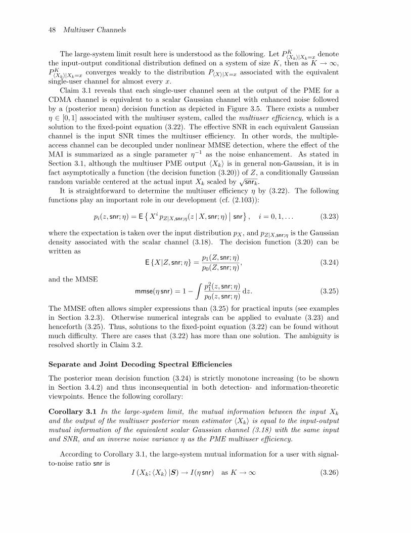
48 Multiuser Channels
The large-system limit result here is understood as the following. Let PK〈Xk〉|Xk=x denote
the input-output conditional distribution defined on a system of size K, then as K → ∞,PK〈Xk〉|Xk=x converges weakly to the distribution P〈X〉|X=x associated with the equivalent
single-user channel for almost every x.Claim 3.1 reveals that each single-user channel seen at the output of the PME for a
CDMA channel is equivalent to a scalar Gaussian channel with enhanced noise followedby a (posterior mean) decision function as depicted in Figure 3.5. There exists a numberη ∈ [0, 1] associated with the multiuser system, called the multiuser efficiency, which is asolution to the fixed-point equation (3.22). The effective SNR in each equivalent Gaussianchannel is the input SNR times the multiuser efficiency. In other words, the multiple-access channel can be decoupled under nonlinear MMSE detection, where the effect of theMAI is summarized as a single parameter η−1 as the noise enhancement. As stated inSection 3.1, although the multiuser PME output 〈Xk〉 is in general non-Gaussian, it is infact asymptotically a function (the decision function (3.20)) of Z, a conditionally Gaussianrandom variable centered at the actual input Xk scaled by
√snrk.
It is straightforward to determine the multiuser efficiency η by (3.22). The followingfunctions play an important role in our development (cf. (2.103)):
pi(z, snr; η) = E{
Xi pZ|X,snr;η(z |X, snr; η)∣∣ snr
}, i = 0, 1, . . . (3.23)
where the expectation is taken over the input distribution pX , and pZ|X,snr;η is the Gaussiandensity associated with the scalar channel (3.18). The decision function (3.20) can bewritten as
E {X|Z, snr; η} =p1(Z, snr; η)p0(Z, snr; η)
, (3.24)
and the MMSE
mmse(η snr) = 1−∫
p21(z, snr; η)
p0(z, snr; η)dz. (3.25)
The MMSE often allows simpler expressions than (3.25) for practical inputs (see examplesin Section 3.2.3). Otherwise numerical integrals can be applied to evaluate (3.23) andhenceforth (3.25). Thus, solutions to the fixed-point equation (3.22) can be found withoutmuch difficulty. There are cases that (3.22) has more than one solution. The ambiguity isresolved shortly in Claim 3.2.
Separate and Joint Decoding Spectral Efficiencies
The posterior mean decision function (3.24) is strictly monotone increasing (to be shownin Section 3.4.2) and thus inconsequential in both detection- and information-theoreticviewpoints. Hence the following corollary:
Corollary 3.1 In the large-system limit, the mutual information between the input Xk
and the output of the multiuser posterior mean estimator 〈Xk〉 is equal to the input-outputmutual information of the equivalent scalar Gaussian channel (3.18) with the same inputand SNR, and an inverse noise variance η as the PME multiuser efficiency.
According to Corollary 3.1, the large-system mutual information for a user with signal-to-noise ratio snr is
I (Xk; 〈Xk〉 |S) → I(η snr) as K →∞ (3.26)

3.2 Model and Summary of Results 49
where the mutual information I(·) as a function of the SNR is consistent with the definition(2.9) in Chapter 2, i.e.,
I(η snr) = D(pZ|X,snr;η || pZ|snr;η | pX), (3.27)
where pZ|snr;η is the marginal probability distribution of the output of channel (3.18). Theoverall spectral efficiency under suboptimal separate decoding is the sum of the single-usermutual informations divided by the dimensionality of the CDMA channel, which is simply
Csep(β) = β E {I(η snr)} . (3.28)
The optimal spectral efficiency under joint decoding is greater than (3.28), where the dif-ference is given by the following:
Claim 3.2 The gain of optimal joint decoding over multiuser posterior mean estimationfollowed by separate decoding in the large-system spectral efficiency of the multiple-accesschannel (3.4) is determined by the PME multiuser efficiency η as3
Cjoint(β)− Csep(β) =12(η − 1− log η) = D (N (0, η) || N (0, 1)) . (3.29)
In other words, the spectral efficiency under joint decoding is
Cjoint(β) = β E {I(η snr)}+12(η − 1− log η). (3.30)
In case of multiple solutions to (3.22), the PME multiuser efficiency η is the one that givesthe smallest spectral efficiency under optimal joint decoding.
Indeed, Muller’s conjecture on the mutual information loss [71] is true for arbitraryinputs and SNRs. Incidentally, the loss is identified as a (Kullback-Leibler) divergencebetween two Gaussian distributions.
The fixed-point equation (3.22), which is obtained using the replica method, may havemultiple solutions. This is known as phase coexistence in statistical physics. Among thosesolutions, the PME multiuser efficiency is the thermodynamically dominant one that givesthe smallest value of the joint decoding spectral efficiency (3.30). It is the solution thatcarries relevant operational meaning in the communication problem. In general, as thesystem parameters (such as the load) change, the dominant solution may switch from oneof the coexisting solutions to another. This is known as phase transition (refer to Section3.6 for numerical examples).
Equal-power Gaussian input is the first known case that admits a closed form solutionfor the multiuser efficiency [112] and henceforth also the spectral efficiencies. The spectralefficiencies under joint and separate decoding were found for Gaussian inputs with fadingin [85], and then found implicitly in [96] and later explicitly [72] for equal-power userswith binary inputs. Formulas (3.28) and (3.30) give general formulas for arbitrary inputdistributions and received powers.
Interestingly, the spectral efficiencies under joint and separate decoding are also relatedby an integral equation. Even more so is the proof based on the central formula that linksmutual information and MMSE in Chapter 2.
3Note that natural logarithm is assumed throughout.

50 Multiuser Channels
Theorem 3.1 For every input distribution PX ,
Cjoint(β) =∫ β
0
1β′
Csep(β′) dβ′. (3.31)
Proof: Since Cjoint(0) = 0, it suffices to show
βddβ
Cjoint(β) = Csep(β). (3.32)
By (3.28) and (3.30), it is enough to show
βddβ
E {I(η snr)}+12
ddβ
[η − 1− log η] = 0. (3.33)
Noticing that η is a function of β, (3.33) is equivalent to
ddη
E {I(η snr)}+12β
(1− η−1
)= 0. (3.34)
By the central formula that links the mutual information and MMSE in Gaussian channels(Theorem 2.1),
ddη
I(ηsnr) =snr
2mmse(η snr). (3.35)
Thus (3.34) holds as η satisfies the fixed-point equation (3.22).
An interpretation of Theorem 3.1 through mutual information chain rule is given inSection 3.2.6.
Generalized Posterior Mean Estimation
Given ξ > 0, consider a postulated scalar Gaussian channel similar to (3.18) with inputsignal-to-noise ratio snr and inverse noise variance ξ:
Z =√
snr X +1√ξ
U (3.36)
where U ∼ N (0, 1) is independent of X. Let the input distribution to this postulated chan-nel be qX . Denote the underlying measure of the postulated system by q. A retrochannel ischaracterized by the posterior probability distribution qX|Z,snr;ξ, namely, it takes in an inputZ and outputs a random variable X according to qX|Z,snr;ξ. Note that the retrochannel isnothing but a materialization of the Bayes posterior distribution. The PME estimate of Xgiven Z is therefore the posterior mean under the measure q:
〈X〉q = Eq {X | Z, snr; ξ} . (3.37)
Consider now a concatenation of the scalar Gaussian channel (3.18) and the retrochannelas depicted in Figure 3.6. Let the input to the Gaussian channel (3.18) be denoted by X0 todistinguish it from the output X of the retrochannel. The probability law of the compositechannel is determined by snr and two parameters η and ξ. Let the generalized PME estimatebe defined as in (3.37). We define the mean-square error of the estimate as
mse(snr; η, ξ) = E
{(X0 − 〈X〉q
)2∣∣∣∣ snr; η, ξ
}. (3.38)

3.2 Model and Summary of Results 51
-X0
∼ pX
⊗√
snr
6
-⊕?
N(0, η−1
)-Z PME
Eq{X| · , snr; ξ} 〈X〉q
X
•
-
-
-RetrochannelqX|Z,snr;ξ
Figure 3.6: The equivalent single-user Gaussian channel, posterior mean estimator andretrochannel.
We also define the variance of the retrochannel as
var(snr; η, ξ) = E
{(X − 〈X〉q
)2∣∣∣∣ snr; η, ξ
}. (3.39)
Note that in the special case where q ≡ p and σ = 1, the postulated channel is identical tothe actual channel, and consequently
mse(snr;x, x) = var(snr;x, x) = mmse(x snr), ∀x. (3.40)
We claim the following for the generalized multiuser PME.
Claim 3.3 Let the generalized posterior mean estimator of the multiuser channel (3.4) bedefined by (3.6) parameterized by the postulated input distribution qX and noise level σ.Then, in the large-system limit, the distribution of the multiuser detection output 〈Xk〉qconditioned on Xk = x being transmitted with signal-to-noise ratio snrk is identical to thedistribution of the generalized PME 〈X〉q of the equivalent scalar Gaussian channel (3.18)conditioned on X = x being transmitted with input signal-to-noise ratio snr = snrk, where themultiuser efficiency η and the inverse noise variance ξ of the postulated scalar channel (3.36)satisfy the coupled equations:
η−1 = 1 + β E {snr ·mse(snr; η, ξ)} , (3.41a)ξ−1 = σ2 + β E {snr · var(snr; η, ξ)} , (3.41b)
where the expectations are taken over Psnr. In case of multiple solutions to (3.41), (η, ξ) ischosen to minimize the free energy expressed as
F =− E
{∫pZ|snr;η(z|snr; η) log qZ|snr;ξ(z|snr; ξ) d z
}− 1
2log
2π
ξ− ξ
2η+
σ2ξ(η − ξ)2βη
+12β
(ξ − 1− log ξ) +12β
log(2π) +ξ
2βη.
(3.42)
Claim 3.3 is a generalization of Claim 3.1 to the case of generalized multiuser PME.The multiuser detector in this case is parameterized by (qX , σ). Nonetheless, the single-userchannel seen at the output of the generalized PME is equivalent to a degraded Gaussianchannel followed by a decision function. However, the multiuser efficiency, same for all

52 Multiuser Channels
users, is now a solution to the coupled fixed-point equations (3.41), which is obtained usingthe replica method to be shown later. In case of multiple solutions, only the parameters(η, ξ) that minimize the free energy (3.42) conform with the operational meaning of thecommunication system.
The decision function (3.37) is akin to (3.7):
Eq {X | Z, snr; ξ} =q1(Z, snr; ξ)q0(Z, snr; ξ)
(3.43)
whereqi(z, snr; ξ) = Eq
{Xi qZ|X,snr;ξ(z|X, snr; ξ)
∣∣ snr}
, i = 0, 1, . . . . (3.44)
Some algebra leads to
mse(snr; η, ξ) = 1 +∫
p0(z, snr; η)q21(z, snr; ξ)
q20(z, snr; ξ)
− 2p1(z, snr; η)q1(z, snr; ξ)q0(z, snr; ξ)
dz (3.45)
and
var(snr; η, ξ) =∫
p0(z, snr; η)q0(z, snr; ξ)q2(z, snr; ξ)− q2
1(z, snr; ξ)q20(z, snr; ξ)
dz. (3.46)
Using (3.45) and (3.46), it is in general viable to find solutions to (3.41) numerically. Sincethe decision function (3.43) is strictly monotone, the following result is straightforward:
Corollary 3.2 In the large-system limit, the mutual information between one user’s inputsymbol and the output of the generalized multiuser posterior mean estimator for this useris equal to the input-output mutual information of the equivalent scalar Gaussian chan-nel (3.18) with the same input distribution and SNR, and an inverse noise variance η asthe multiuser efficiency given by Claim 3.3.
3.2.5 Recovering Known Results
As shown in 3.2.3, several well-known multiuser detectors can be regarded as the generalizedPME with appropriate parameters. Thus many previously known results can be recoveredas special case of the new findings in Section 3.2.4.
Linear Detectors
For linear multiuser detectors, standard Gaussian prior is postulated for the generalizedmultiuser PME as well as the postulated scalar channel (3.36). Since the input Z andoutput X of the retrochannel are jointly Gaussian (refer to Figure 3.6), the PME is simplya linear attenuator (cf. (2.11)):
〈X〉q =ξ√
snr
1 + ξsnrZ. (3.47)
The variance of X conditioned on Z is independent of Z. Hence the variance of theretrochannel output is independent of η (cf. (2.12)):
var(snr; η, ξ) =1
1 + ξsnr. (3.48)

3.2 Model and Summary of Results 53
From Claim 3.3, one finds that ξ is the solution to
ξ−1 = σ2 + β E
{snr
1 + ξsnr
}. (3.49)
Meanwhile, the mean-square error is
E
{(X0 − 〈X〉q
)2}
= E
{[X0 −
ξ√
snr
1 + ξsnr
(√snrX0 +
1√
ηN
)]2}
(3.50)
=η + ξ2snr
η(1 + ξsnr)2. (3.51)
After some algebra, the multiuser efficiency is determined as
η = ξ + ξ (σ2 − 1)[1 + β E
{snr
(1 + ξsnr)2
}]−1
. (3.52)
Clearly, the large-system multiuser efficiency of such a linear detector is independent of theinput distribution.
For the matched filter, we let the postulated noise level σ → ∞. One finds ξσ2 → 1by (3.49) and consequently, the multiuser efficiency of matched filter is [112]
η(mf) =1
1 + β E {snr}. (3.53)
In case of MMSE detector, the control parameter σ = 1. By (3.52), one finds that η = ξand by (3.49), the multiuser efficiency η satisfies the Tse-Hanly equation [99, 105]:
η−1 = 1 + β E
{snr
1 + ηsnr
}, (3.54)
which has a unique positive solution η(mmse).In case of decorrelator, the control parameter σ → 0. If β < 1, then (3.49) gives ξ →∞
and ξσ2 → 1− β, and the multiuser efficiency is found as η = 1− β by (3.52) regardless ofthe SNR distribution. If β > 1, and assuming the generalized form of the decorrelator asthe Moore-Penrose inverse of the correlation matrix [112], then ξ is the unique solution to
ξ−1 = β E
{snr
1 + ξsnr
}(3.55)
and the multiuser efficiency is found by (3.52) with σ = 0. In the special case of equal SNRfrom all users, an explicit expression can be found [23, 39]
η(dec) =β − 1
β + snr(β − 1)2, β > 1. (3.56)
By Corollary 3.2, the mutual information with input distribution pX for a user withsignal-to-noise ratio snr under linear multiuser detection is the input-output mutual infor-mation of the scalar Gaussian channel (3.18) with the same input:
I(X; 〈X〉q |snr) = I(η snr), (3.57)

54 Multiuser Channels
where η depends on which type of linear detector is in use. Gaussian priors are known toachieve the capacity:
C(snr) =12
log(1 + η snr). (3.58)
By Corollary 3.2, the total spectral efficiency under Gaussian inputs is expressed in termsof the linear MMSE multiuser efficiency:
C(Gaussian)joint =
β
2E{
log(1 + η(mmse)snr
)}+
12
(η(mmse) − 1− log η(mmse)
). (3.59)
This is exactly Shamai and Verdu’s result for fading channels [85].
Optimal Detectors
Using the actual input distribution pX as the postulated priors of the generalized PMEresults in optimum multiuser detectors. In case of the jointly optimum detector, the pos-tulated noise level σ = 0, and (3.41) becomes
η−1 = 1 + β E {snr ·mse(snr; η, ξ)} , (3.60a)ξ−1 = β E {snr · var(snr; η, ξ)} , (3.60b)
where mse(·) and var(·) are given by (3.45) and (3.46) with qi(z, snr;x) = pi(z, snr;x), ∀x.The parameters have to be solved numerically.
In case of the individually optimal detector, σ = 1. It is clear that the postulatedmeasure qX,Y |S is identical to the true measure pX,Y |S . In the equivalent scalar channeland its retrochannel, the parameters satisfy
η−1 = 1 + β E {snr ·mse(snr; η, ξ)} , (3.61a)ξ−1 = 1 + β E {snr · var(snr; η, ξ)} . (3.61b)
We take the symmetric solution η = ξ due to (3.40). The multiuser efficiency η is thusthe solution to the fixed-point equation (3.22) given in Claim 3.1. It should be cautionedthat (3.61) may have other solutions with η 6= ξ in the unlikely case that replica symmetrydoes not hold.
It is of practical interest to find the spectral efficiency under the constraint that the inputsymbols are antipodally modulated as in the popular BPSK. In this case, the distributionpX(x) = 1/2, x = ±1, maximizes the mutual information. The MMSE is given by (2.16).By Claim 3.1, The multiuser efficiency, η(b), where the superscript (b) stands for binaryinputs, is a solution to the fixed-point equation:
η−1 = 1 + β E
{snr
[1−
∫1√2π
e−z2
2 tanh (ηsnr − z√
ηsnr) dz
]}, (3.62)
which is a generalization to unequal-power distribution [39] of an earlier result on equalSNRs due to Tanaka [96]. The single-user channel capacity for a user with signal-to-noiseratio snr is the same as that obtained by Muller and Gerstacker [72] and is given by (2.17)with snr replaced by η(b) snr. The total spectral efficiency of the CDMA channel subject tobinary inputs is thus
C(b)joint =β E
{η(b) snr −
∫1√2π
e−z2
2 log cosh(
η(b)snr − z
√η(b)snr
)dz
}+
12
[η(b) − 1− log η(b)
],
(3.63)
which is also a generalization in [39] of Tanaka’s implicit result [96].

3.2 Model and Summary of Results 55
3.2.6 Discussions
Successive Interference Cancellation
Theorem 3.1 is an outcome of the chain rule of mutual information, which holds for allinputs and arbitrary number of users:
I(X;Y |S) =K∑
k=1
I(Xk;Y |S, Xk+1, . . . , XK). (3.64)
The left hand side of (3.64) is the total capacity of the multiuser channel. Each summand onthe right hand side of (3.64) is a single-user capacity over the multiuser channel conditionedon the symbols of previously decoded users. As argued in the following, the limit of (3.64)as K →∞ becomes the integral equation (3.31).
We conceive an interference canceler that decodes the users successively in which reliablydecoded symbols as well as the generalized PME estimates of the yet undecoded usersare used to reconstruct the interference for cancellation. Since the error probability ofintermediate decisions vanishes with code block-length, the MAI from decoded users areasymptotically completely removed. Without loss of generality assume that the users aredecoded in reverse order, then the generalized PME for user k sees only k − 1 interferingusers. Hence the performance for user k under successive decoding is identical to that underparallel separate decoding in a CDMA system with k instead of K users. Nonetheless,the equivalent single-user channel for each user is Gaussian by Claim 3.3. The multiuserefficiency experienced by user k is η
(kL
)where we use the fact that it is a function of the
load kL seen by the generalized PME for user k. Following (3.26), the single-user capacity
for user k is therefore
I
(η
(k
L
)snrk
). (3.65)
Assuming that the i.i.d. snrk are not dependent on the indexes k, the overall spectralefficiency under successive decoding converges almost surely:
1L
K∑k=1
I
(η
(k
L
)snrk
)→ E
{∫ β
0I(β′ snr) dβ′
}. (3.66)
Note that the above result on successive decoding is true for arbitrary input distributionpX and generalized PME detectors. In the special case of the PME, for which the postulatedsystem is identical to the actual one, the right hand side of (3.66) is equal to Cjoint(β) byTheorem 3.1. We can summarize this principle as:
Proposition 3.1 In the large-system limit, successive decoding with a PME front endagainst yet undecoded users achieves the optimal CDMA channel capacity under arbitraryinput distributions.
Proposition 3.1 is a generalization of the previous result that a successive canceler witha linear MMSE front end against undecoded users achieves the capacity of the CDMAchannel under Gaussian inputs [102, 80, 105, 2, 70, 33]. In the special case of Gaussianinputs, however, the optimality is known to hold for any finite number of users [102, 105].

56 Multiuser Channels
���������
�����
���������
�� � �������� ���
� ��� � � � � � ��� � � � �
!" #
! $&%�'(%�)+*-,/.10�%�235476! 89 9;: << = ! >
Figure 3.7: A canonical interference canceler equivalent to the single-user Gaussian channel.
Parallel Interference Cancellation Puzzle
We give a quick and specious interpretation of the large-system results. The assumptionsthat will be made are erroneous, hence the interpretation is fundamentally rootless. How-ever, the argument leads surprisingly to the correct result. We suspect that this interpreta-tion can be fixed to obtain a correct justification of the results. The author has failed butnonetheless would like to include the argument in case the reader may turn it to a success.
We construct without loss of generality an estimator for user 1 using interference can-cellation as depicted in Figure 3.7. Let 〈X2〉q , . . . , 〈XK〉q be the generalized PME estimatesfor user 2 through user K. A decision statistic for user 1 can be generated by first subtract-ing the reconstructed interferences using those estimates and then matched filtering withrespect to user 1’s spreading sequence:
Z1 =√
snr1X1 +K∑
k=2
s>1sk√
snrk
(Xk − 〈Xk〉q
)+ N1 (3.67)
where N1 is a standard Gaussian random variable. If the desired symbol X1, the Gaussiannoise N1, and the residual errors
(Xk − 〈Xk〉q
)were independent, by virtue of the central
limit theorem, the sum of the residual MAI and Gaussian noise converges to a Gaussianrandom variable as K → ∞. The variance of Xk − 〈Xk〉q is mse(snrk; η, ξ) by Claim 3.3.The variance of the total interference in (3.67) is therefore
1 + β E {snr ·mse(snr; η, ξ)} , (3.68)
which, by the fixed-point equation (3.41a) in Claim 3.3, is equal to η−1. Thus if theindependence assumption were valid, we would have found a degraded Gaussian channelfor user 1 equivalent to the single-user channel as shown in Figure 3.6. That is also to saythat, given the generalized PME estimates of all interfering users, the interference cancelerproduces for the desired user an estimate that is as good as the generalized PME output. Wecan also argue that every user enjoys the same efficiency since otherwise users with worseefficiency may benefit from users with better efficiency until an equilibrium is reached.Roughly speaking, the generalized PME output is a “fixed-point” of a parallel interferencecanceler. The multiuser efficiency, in a sense, is the outcome of such an equilibrium.
It should be emphasized that the above interpretation does not hold due to the erroneousindependence assumption. In particular, s>1sk are not independent, albeit uncorrelated, forall k. Also, 〈Xk〉q is dependent on the desired signal X1 and the noise N1. This is evidentin the special case of linear MMSE detection. One is tempted to fix the argument by first

3.3 Multiuser Communications and Statistical Physics 57
decorrelating the residual errors, the desired symbol and the noise to satisfy the requirementof central limit theorem. It seems to be possible because correlation between the MAI andthe desired signal may neutralize the correlations among the components of the MAI aswell as with the noise. The author has failed to show this.
3.3 Multiuser Communications and Statistical Physics
In this section, we prepare the reader with concepts and methodologies that will be neededto prove the results given in Section 3.2.4. The replica method, which we will make useof, was originally developed in spin glass theory in statistical physics [22]. Although onecan work with the mathematical framework only and avoid foreign concepts, we believeit is more enlightening to draw an equivalence in between multiuser communications andmany-body problems in statistical physics. Such an analogy is first seen in a primitive formin [96] and will be developed to a full generality here.
3.3.1 A Note on Statistical Physics
Let the microscopic state of a system be described by the configuration of some K variablesas a vector x. The Hamiltonian is a function of the configuration, denoted by H(x) . Thestate of the system evolves over time according to some physical laws, and after long enoughtime it reaches thermal equilibrium. The time average of an observable quantity can beobtained by averaging over the ensemble of the states. In particular, the energy of thesystem is
E =∑x
p(x)H(x) (3.69)
where p(x) is the probability of the system being found in configuration x. In other words, asfar as the macroscopic properties are concerned, it suffices to describe the system statisticallyinstead of solving the exact dynamic trajectories. Another fundamental quantity is theentropy, defined as
S = −∑x
p(x) log p(x). (3.70)
It is assumed that the system is not isolated and may interact with the surroundings. As aresult, at thermal equilibrium, the energy of the system remains a constant and the entropyis the maximum possible.
Given the energy E , one can use the Lagrange multiplier method to show that the equi-librium probability distribution that maximizes the entropy is the Boltzmann distribution
p(x) = Z−1 exp[− 1
TH(x)
](3.71)
where
Z =∑x
exp[− 1
TH(x)
](3.72)
is the partition function, and the parameter T is the temperature, which is determined bythe energy constraint (3.69). The system is found in each configuration with a probabilitythat is negative exponential in the Hamiltonian associated with the configuration. The mostprobable configuration is the ground state which has the minimum Hamiltonian.

58 Multiuser Channels
SourcepX
-X0 ChannelpY |X,S
-Y•
-
Generalized CMEEq{X| · ,S}
-〈X〉q
RetrochannelqX|Y ,S
- X
Figure 3.8: A canonical channel, its corresponding retrochannel, and the generalized PME.
One particularly useful macroscopic quantity of the thermodynamic system is the freeenergy, defined as
E − T S. (3.73)
Since the entropy is the maximum at equilibrium, the free energy is at its minimum. Us-ing (3.69)–(3.72), one finds that the free energy at equilibrium can also be expressed as−T log Z. The free energy is often the starting point for calculating macroscopic propertiesof a thermodynamic system.
3.3.2 Communications and Spin Glasses
The statistical inference problem faced by an estimator can be described as follows. A(vector) source symbol X0 is drawn according to a prior distribution pX . The channelresponse to the input X0 is an output Y generated according to a conditional probabilitydistribution pY |X,S where S is the channel state. The estimator would like to draw someconclusion about the original symbol X0 upon receiving Y using knowledge about thestate S. Naturally, the posterior distribution pX|Y ,S is central in the statistical inferenceproblem.
If pX|Y ,S is revealed to the estimator, we have the posterior mean estimator, which isoptimal in mean-square sense. One may choose, however, to supply any posterior distribu-tion qX|Y ,S in lieu of pX|Y ,S , henceforth resulting a generalized PME: 〈X〉q = Eq{X|Y ,S}.As shown in Section 3.2.3, the freedom in choosing the postulated measure allows treatmentof various detection techniques in a uniform framework.
It is conceptually helpful here to also introduce the retrochannel induced by the postu-lated system. The multiuser channel, the generalized multiuser PME, and the associatedretrochannel are depicted in Figure 3.8 (to be compared with its single-user counterpart inFigure 3.6). Upon receiving a signal Y with a channel state S, the retrochannel outputs arandom vector according to the probability distribution qX|Y ,S , which is induced by the pos-tulated prior distribution qX and the postulated conditional distribution qY |X,S . Clearly,given (Y ,S), the generalized PME output 〈X〉q is the expected value of the retrochanneloutput X.
In the multiple-access channel (3.4), the channel state consists of the spreading sequencesand the SNRs, collectively represented by matrix S. The conditional distribution pY |X,S
is a Gaussian density (3.16). In this work, the postulated channel (3.17) differs from theactual one only in the noise variance. Assuming an input distribution of qX , the posteriordistribution of the postulated channel can be obtained by using the Bayes formula (cf. (3.7))

3.3 Multiuser Communications and Statistical Physics 59
as
qX|Y ,S(x|y,S) =[qY |S(y|S)
]−1qX(x)
(2πσ2
)−L2 exp
[− 1
2σ2‖y − Sx‖2
](3.74)
where
qY |S(y|S) =(2πσ2
)−L2 Eq
{exp
[− 1
2σ2‖y − SX‖2
] ∣∣∣∣ S
}(3.75)
and where the expectation in (3.75) is taken conditioned on S over X with distribution qX .Interestingly, we can associate the posterior probability distribution (3.74) with the
characteristics of a thermodynamic system called spin glass. We believe this work is thefirst to draw this analogy in the general setting, although in certain special cases the ar-gument is found in Tanaka’s important paper [96]. A spin glass is a system consisting ofmany directional spins, in which the interaction of the spins is determined by the so-calledquenched random variables whose values are determined by the realization of the spin glass.4
Let the microscopic state of a spin glass be described by a K-dimensional vector x. Letthe quenched random variables be denoted by (y,S). The system can be understood as Krandom spins sitting in quenched randomness (y,S). The basic quantity characterizing amicroscopic state is the Hamiltonian, which is a function of the configuration dependent onthe quenched randomness, denoted by Hy,S(x). At thermal equilibrium, the spin glass isfound in each configuration with the Boltzmann distribution:
q(x|y,S) = Z−1(y,S) exp[− 1
THy,S(x)
](3.76)
where
Z(y,S) =∑x
exp[− 1
THy,S(x)
](3.77)
is the partition function. This equilibrium distribution maximizes the entropy subject toenergy constraint.
The reader may have noticed the similarity between (3.74)–(3.75) and (3.76)–(3.77).Indeed, if the temperature T = 1 in (3.76)–(3.77) and that the Hamiltonian is defined as
Hy,S(x) =L
2log(2πσ2
)+
12σ2
‖y − Sx‖2 − log qX(x), (3.78)
then
q(x|y,S) = qX|Y ,S(x|y,S), (3.79)Z(y,S) = qY |S(y|S). (3.80)
In other words, by defining an appropriate Hamiltonian, the configuration distribution of thespin glass at equilibrium is identical to the posterior probability distribution associated witha multiuser communication system. Precisely, the probability that the transmitted symbolis x under the postulated model, given the observation y and the channel state S, is equalto the probability that the spin glass is at configuration x, given the values of the quenched
4An example is a system consisting molecules with magnetic spins that evolve over time, while thepositions of the molecules that determine the amount of interactions are random (disordered) but remainfixed for each concrete instance as in a piece of glass (hence the name of spin glass).

60 Multiuser Channels
random variables (Y ,S) = (y,S). It is interesting to note that Gaussian distribution is anatural Boltzmann distribution with squared Euclidean norm as the Hamiltonian.
The quenched randomness (Y ,S) takes a specific distribution in our problem, i.e.,(Y ,S) is a realization of the received signal and channel state matrix according to the priorand conditional distributions that underlie the “original” spins. Indeed, the communicationsystem depicted in Figure 3.8 can be also understood as a spin glass X under physical law qsitting in the quenched randomness caused by another spin glass X0 under physical law p.The channel corresponds to the random mapping from a given spin glass configuration toan induced quenched randomness. Conversely, the retrochannel corresponds to the randommechanism that maps some quenched randomness into an induced spin glass configuration.
The free energy of the thermodynamic (or communication) system is obtained as:
−T log Z(Y ,S). (3.81)
In the following, we show some useful properties of the free energy and associate it with thespectral efficiency of communication systems.
3.3.3 Free Energy and Self-averaging Property
The free energy (3.81) with T = 1 and normalized by the number of users is (via (3.80))
− 1K
log qY |S(Y |S). (3.82)
As mentioned in Section 3.1, the randomness in (3.82) vanishes as K → ∞ due to theself-averaging assumption. As a result, the free energy normalized by the number of usersconverges in probability to its expected value over the distribution of the quenched randomvariables (Y ,S) in the large-system limit, which is denoted by F ,
F = − limK→∞
E
{1K
log Z(Y ,S)}
. (3.83)
Hereafter, by the free energy we refer to the large-system limit F , which we will calculatein Section 3.4.
The reader should be cautioned that for disordered systems, thermodynamic quantitiesmay or may not be self-averaging [14]. The self-averaging property remains to be provedor disproved in the CDMA context. This is a challenging problem on its own. In this workwe take the self-averaging property for granted with a good faith that it be correct. Again,we believe that even if the self-averaging property breaks down, the main results in thischapter are good approximations and still useful to some extent in practice.
The self-averaging property resembles the asymptotic equipartition property (AEP) ininformation theory [17]. An important consequence is that a macroscopic quantity of athermodynamic system, which is a function of a large number of random variables, maybecome increasingly predictable from merely a few parameters independent of the realizationof the random variables as the system size grows without bound. Indeed, the macroscopicquantity converges in probability to its ensemble average in the thermodynamic limit.
In the CDMA context, the self-averaging property leads to a strong consequence thatfor almost all realizations of the received signal and the spreading sequences, macroscopicquantities such as the BER, the output SNR and the spectral efficiency, averaged overdata, converge to deterministic quantities in the large-system limit. Previous work (e.g.

3.3 Multiuser Communications and Statistical Physics 61
[105, 99, 44]) has shown convergence of performance measures for almost all spreadingsequences. The self-averaging property results in convergence of empirical measures oferror performance and information rate, which holds for almost all realizations of the dataand noise.
3.3.4 Spectral Efficiency of Jointly Optimal Decoding
This section associates the optimal spectral efficiency of a multiuser communication systemwith the free energy of a corresponding spin glass. This is again a full generalization of anobservation by Tanaka [96] in special cases. In fact, the analogy between free energy andinformation-theoretic quantities has been noticed in belief propagation [117], coding [101]and optimization problems [11] as well.
For a fixed input distribution pX , the total mutual information under joint decoding is
I(X;Y |S) = E
{log
pY |X,S(Y |X,S)pY |S(Y |S)
∣∣∣∣ S
}(3.84)
where the expectation is taken over the conditional joint distribution pX,Y |S . Since thechannel characteristic given by (3.16) is a standard L-dimensional Gaussian density, onehas
E{
log pY |X,S(Y |X,S)∣∣ S}
= −L
2log(2πe). (3.85)
Suppose that the postulated measure q is the same as the actual measure p, then by (3.80),(3.84) and (3.85), the spectral efficiency in nats per degree of freedom achieved by optimaljoint decoding is
C(S) =1L
I(X;Y |S) (3.86)
= −β E
{1K
log Z(Y ,S)∣∣∣∣S}− 1
2log(2πe). (3.87)
To calculate (3.87) is formidable for an arbitrary realization of S but due to the self-averaging property, the spectral efficiency converges in probability as K, N →∞ to
C = βF|q=p −12
log(2πe) (3.88)
where F is defined in (3.83). Note that the constant term in (3.88) can be removed byredefining the partition function up to a constant coefficient. In either way, the spectral ef-ficiency under optimal joint decoding is affine in the free energy under a postulated measureq identical to the true measure p.
3.3.5 Separate Decoding
In case of a multiuser detector front end, one is interested in the distribution of the detectionoutput 〈Xk〉q conditioned on the input X0k. Here, X0k is used to denote the input to theCDMA channel to distinguish it from the retrochannel output Xk. Our approach is tocalculate joint moments
E{
Xj0k 〈Xk〉iq
∣∣∣ S}
, i, j = 0, 1, . . . (3.89)

62 Multiuser Channels
pX -X0 pY |X,S
6S
-Y Retrochannel 1pX|Y ,S
Retrochannel u
S
--
-
X1
X2
Xu
6S
Figure 3.9: The replicas of the retrochannel.
and then infer the distribution of (〈Xk〉q −X0k). In the spin glass context, one may inter-pret (3.89) as the joint moments of the spins X0 that induced the quenched randomness,and the conditional expectation of the induced spins X. The calculation of (3.89) is againformidable due to its dependence on the channel state, but in the large-system limit, theresult is surprisingly simple. Due to the self-averaging property, the moments also convergein probability, and it suffices to calculate the moments with respect to the joint distributionof the spins and the quenched randomness as
limK→∞
E{
Xj0k 〈Xk〉iq
}. (3.90)
Note that X0 → (Y ,S) → X is a Markov chain. It can be shown that (3.90) is equivalentto
limK→∞
E{
Xj0k Xi
k
}, (3.91)
which turns out to be easier to calculate by studying the free energy associated with amodified version of the partition function (3.75). More on this later.
The mutual information between the input and the output of a multiuser detector frontend for an arbitrary user k is given by
I(X0k; 〈Xk〉q |S), (3.92)
which can be derived once the input-output relationship is known. It will be shown thatconditioning on the channel state S is asymptotically inconsequential.
We have distilled our problems under both joint and separate decoding to finding someensemble averages, namely, the free energy (3.83) and the moments (3.91). In order tocalculate these quantities, we resort to a powerful technique developed in the theory of spinglass, the heart of which is sketched in the following subsection.
3.3.6 Replica Method
The replica method was introduced to the field of multiuser detection by Tanaka to analyzeoptimal detectors under equal power Gaussian or binary input. In the following we outlinethe method in a more general setting following Tanaka’s pioneering work [96].
The expected value of the logarithm in (3.83) can be reformulated as
F = − limK→∞
1K
limu→0
∂
∂ulog E {Zu(Y ,S)} . (3.93)

3.3 Multiuser Communications and Statistical Physics 63
The equivalence of (3.83) and (3.93) can be easily verified by noticing that
limu→0
∂
∂ulog E {Θu} = lim
u→0
E {Θu log Θ}E {Θu}
= E {log Θ} , ∀Θ. (3.94)
For an arbitrary integer replica number u, we introduce u independent replicas of theretrochannel (or the spin glass) with the same received signal Y and channel state matrixS as depicted in Figure 3.9. Conditioned on (Y ,S), Xa are independent. By (3.80), thepartition function of the replicated system is
Zu(y,S) = Eq
{u∏
a=1
qY |X,S(y|Xa,S)
∣∣∣∣∣ S
}(3.95)
where the expectation is taken over the i.i.d. symbols {Xak|a = 1, . . . , u, k = 1, . . . ,K},with distribution qX . Note that Xak are i.i.d. since Y = y is given. We can henceforthevaluate
− limK→∞
1K
log E {Zu(Y ,S)} (3.96)
as a function of the integer u. The replica trick assumes that the resulting expression isalso valid for an arbitrary real number u and finds the derivative at u = 0 as the freeenergy. Besides validity of continuing to non-integer values of the replica number u, it isalso necessary to assume that the two limits in (3.93) can be exchanged in order.
It remains to calculate (3.96). Note that (Y ,S) is induced by the transmitted symbolsX0. By taking expectation over Y first and then averaging over the spreading sequences,one finds that
1K
log E {Zu(Y ,S)} =1K
log E{
exp[β−1K G
(u)K (Γ,X)
]}(3.97)
where G(u)K is some function of the SNRs and the transmitted symbols and their replicas,
collectively denoted by a K × (u + 1) matrix X = [X0, . . . ,Xu]. By first conditioning onthe correlation matrix Q of ΓX, the central limit theorem helps to reduce (3.97) to
1K
log∫
exp[β−1K G(u)(Q)
]µ
(u)K ( dQ) (3.98)
where G(u) is some function of the (u + 1) × (u + 1) correlation matrix Q, and µ(u)K is the
probability measure of the random matrix Q. Large deviations can be invoked to show thatthere exists a rate function I(u) such that the measure µ
(u)K satisfies
− limK→∞
1K
log µ(u)K (A) = inf
Q∈AI(u)(Q) (3.99)
for all measurable set A of (u + 1)× (u + 1) matrices. Using Varadhan’s theorem [25], theintegral (3.98) is found to converge as K →∞ to
supQ
[β−1 G(u)(Q)− I(u)(Q)]. (3.100)
Seeking the extremum over a (u + 1)2-dimensional space is a hard problem. The techniqueto circumvent this is to assume replica symmetry, namely, that the supremum in Q is

64 Multiuser Channels
symmetric over all replicated dimensions. The resulting supremum is then over merely afew parameters, and the free energy can be obtained.
The replica method is also used to calculate (3.91). Clearly, X0—(Y ,S)—[X1, . . . ,Xu]is a Markov chain. The moments (3.91) are equivalent to
limK→∞
E
{Xj
0k
i∏m=1
Xmk
}(3.101)
which can be readily evaluated by working with a modified partition function akin to (3.95).Detailed replica analysis of the real-valued channel is carried out in Section 3.4. The
complex-valued counterpart is discussed in Section 3.5. As mentioned in Section 3.1, whilewe assume the replica trick and replica symmetry to be valid as well as the self-averagingproperty, their fully rigorous justification is still open mathematical physics.
3.4 Proofs Using the Replica Method
This section proves Claims 3.1–3.3 using the replica method. The free energy is calculatedfirst and hence the spectral efficiency under joint decoding is derived. The joint momentsof the input and multiuser detection output are then found and it is demonstrated that theCDMA channel can be effectively decoupled into single-user Gaussian channels. Thus themultiuser efficiency as well as the spectral efficiency under separate decoding is found.
3.4.1 Free Energy
We will find the free energy by (3.93) and then the spectral efficiency is trivial by (3.88).From (3.95),
E {Zu(Y ,S)} = E
{∫pY |S(y|S)Zu(y,S) dy
}(3.102)
= E
{∫pY |X,S(y|X0,S)
u∏a=1
qY |X,S(y|Xa,S) dy
}(3.103)
where the expectation in (3.103) is taken over the channel state matrix S, the originalsymbol vector X0 (i.i.d. entries with distribution pX), and the replicated symbols Xa,a = 1, . . . , u (i.i.d. entries with distribution qX). Note that S, X0 and Xa are independent.Let X = [X0, . . . ,Xu]. Plugging (3.16) and (3.17) into (3.103),
E {Zu(Y ,S)} =E
{∫(2π)−
L2 (2πσ2)−
uL2 exp
[−1
2‖y − SX0‖2
]×
u∏a=1
exp[− 1
2σ2‖y − SXa‖2
]dy
}.
(3.104)
We glean from the fact that the L dimensions of the CDMA channel are independent andstatistically identical, and write (3.104) as
E {Zu(Y ,S)} =E
[(
2πσ2)−u
2
∫E
{exp
[−1
2
(y − SΓX0
)2]
×u∏
a=1
exp[− 1
2σ2
(y − SΓXa
)2]∣∣∣∣Γ,X
}dy√2π
]L} (3.105)

3.4 Proofs Using the Replica Method 65
where the inner expectation in (3.105) is taken over S = [S1, . . . , SK ], a vector of i.i.d.random variables each taking the same distribution as the random spreading chips Snk.Define the following variables:
Va =1√K
K∑k=1
√snrk SkXak, a = 0, 1, . . . , u. (3.106)
Clearly, (3.105) can be rewritten as
E {Zu(Y ,S)} = E{
exp[LG
(u)K (Γ,X)
]}(3.107)
where
G(u)K (Γ,X) =− u
2log(2πσ2
)+ log
∫E
{exp
[−1
2
(y −
√β V0
)2]
×u∏
a=1
exp[− 1
2σ2
(y −
√β Va
)2]∣∣∣∣Γ,X
}dy√2π
.
(3.108)
Note that given Γ and X, each Va is a sum of K weighted i.i.d. random chips, and henceconverges to a Gaussian random variable as K →∞. In fact, due to a generalization of thecentral limit theorem, V converges to a zero-mean Gaussian random vector with covariancematrix Q where
Qab = E {VaVb | Γ,X} =1K
K∑k=1
snrkXakXbk, a, b = 0, . . . , u. (3.109)
Note that although inexplicit in notation, Qab is a function of {snrk, Xak, Xbk}Kk=1. The
reader is referred to Appendix A.4 for a justification of the asymptotic normality of Vthrough the Edgeworth expansion. As a result,
exp[G
(u)K (Γ,X)
]= exp
[G(u)(Q) +O(K−1)
](3.110)
where
G(u)(Q) =− u
2log(2πσ2
)+ log
∫E
{exp
[(y −
√β V0
)2]
×u∏
a=1
exp[− 1
2σ2
(y −
√β Va
)2]∣∣∣∣Q} dy√
2π,
(3.111)
in which V is a Gaussian random vector with covariance matrix Q. By (3.107) and (3.110),
1K
log E {Zu(Y ,S)} =1K
log E{
exp[L(G(u)(Q) +O
(K−1
))]}(3.112)
=1K
log∫
exp[K β−1 G(u)(Q)
]dµ
(u)K (Q) +O(K−1)(3.113)
where the expectation over the replicated symbols is rewritten as an integral over theprobability measure of the correlation matrix Q, which is expressed as
µ(u)K (Q) = E
u∏
0≤a≤b
δ
(1K
K∑k=1
snrkXakXbk −Qab
) (3.114)

66 Multiuser Channels
where δ(·) is the Dirac function. By Cramer’s theorem, the probability measure of theempirical means Qab defined by (3.109) satisfies, as K →∞, the large deviations propertywith some rate function I(u)(Q) [25]. Note the factor K in the exponent in the integralin (3.113). As K → ∞, the integral is dominated by the maximum of the overall effect ofthe exponent and the rate of the measure on which the integral takes place. Precisely, byVaradhan’s theorem [25],
limK→∞
1K
log E {Zu(Y ,S)} = supQ
[β−1 G(u)(Q)− I(u)(Q)] (3.115)
where the supremum is over all possible Q that can be obtained from varying Xak in (3.109).Let the moment generating function be defined as
M (u)(Q) = E{
exp[snrX>QX
]}(3.116)
where Q is a (u + 1) × (u + 1) symmetric matrix and the expectation in (3.116) is takenover independent random variables snr ∼ Psnr, X0 ∼ pX and X1, . . . , Xu ∼ qX . The rateof the measure µ
(u)K is given by the Legendre-Fenchel transform of the cumulant generating
function (logarithm of the moment generating function) [25]:
I(u)(Q) = supQ
I(u)(Q, Q) (3.117)
= supQ
[tr{
QQ}− log M (u)(Q)
](3.118)
where the supremum is taken with respect to the symmetric matrix Q.In Appendix A.5, (3.111) is evaluated to obtain
G(u)(Q) = −12
log det(I + ΣQ)− 12
log(1 +
u
σ2
)− u
2log(2πσ2
)(3.119)
where Σ is a (u + 1)× (u + 1) matrix:5
Σ =β
σ2 (σ2 + u)
uσ2 −σ2 −σ2 . . . −σ2
−σ2 σ2 + u− 1 −1 . . . −1
−σ2 −1 σ2 + u− 1. . .
...
......
. . . . . . −1
−σ2 −1 . . . −1 σ2 + u− 1
. (3.120)
Note that the lower right u× u block of the matrix in (3.120) is (σ2 + u)Iu −Eu where Iu
denotes the u×u identity matrix and Eu denotes a u×u matrix whose entries are all 1. Itis clear that Σ is invariant if two nonzero indexes are interchanged, i.e., Σ is symmetric inthe replicas.
5For convenience, the index number of all (u + 1)× (u + 1) matrices in this chapter starts from 0.

3.4 Proofs Using the Replica Method 67
By (3.115)–(3.119), one has
limK→∞
1K
log E {Zu(Y ,S)}
= supQ
{β−1 G(u)(Q)− sup
Q
[tr{
QQ}− log M (u)(Q)
]}(3.121)
= supQ
infQ
T (u)(Q, Q) (3.122)
where
T (u)(Q, Q) =− 12β
log det(I + ΣQ)− tr{
QQ}
+ log E{
exp[snrX>QX
]}− 1
2βlog(1 +
u
σ2
)− u
2βlog(2πσ2
).
(3.123)
For an arbitrary Q, we first seek the point of zero gradient with respect to Q and find thatfor a given Q, the extremum in Q satisfies
Q =E{
snrXX>exp[snrX>QX
]}E{
exp[snrX>QX
]} . (3.124)
Let Q∗(Q) be a solution to (3.124), which is a function of Q. Assuming that Q
∗(Q)
is sufficiently smooth, we then seek the point of zero gradient of T (u)(Q, Q
∗(Q)
)with
respect to Q.6 By virtue of the relationship (3.124), one finds that the derivative of Q∗
with respect to Q is inconsequential, and the extremum in Q satisfies
Q = − 1β
(Σ−1 + Q)−1 . (3.125)
It is interesting to note from the resulting joint equations (3.124)–(3.125) that the orderin which the supremum and infimum are taken in (3.122) can be exchanged without harm.The solution
(Q∗, Q
∗)is in fact a saddle point of T (u). Notice that (3.124) can also be
expressed asQ = E
{snrXX>
∣∣∣ Q}
(3.126)
where the expectation is over an appropriately defined measure pX,snr|Q dependent on Q.Solving joint equations (3.124) and (3.125) directly is prohibitive except in the simplest
cases such as qX being Gaussian. In the general case, because of the symmetry in the matrixΣ (3.120), we postulate that the solution to the joint equations satisfies replica symmetry,namely, both Q∗ and Q
∗are invariant if two nonzero replica indexes are interchanged. In
6The formula in footnote 2 on page 10 and the following identity is useful:
∂Q−1
∂x= −Q−1 ∂Q
∂xQ−1.

68 Multiuser Channels
other words, the extremum can be written as
Q∗ =
r m m . . . mm p q . . . q
m q p. . .
......
.... . . . . . q
m q . . . q p
, Q∗
=
c d d . . . dd g f . . . f
d f g. . .
......
.... . . . . . f
d f . . . f g
(3.127)
where r, m, p, q, c, d, f, g are some real numbers.It can be shown that replica symmetry holds in case that the postulated prior qX is Gaus-
sian. Under equal-power binary input and individually optimal detection, Tanaka showedalso the stability of the replica-symmetric solution against replica-symmetry-breaking (RSB)if it is a “stable” solution (i.e., when the parameters satisfies certain condition) [96]. Thus,the replica-symmetric solution is at least a local maximum in such cases. In other cases,stability of replica symmetry can be broken [51]. Unfortunately, there is no known generalcondition for replica symmetry to hold. In this work we assume replica symmetry to holdand limit ourselves to replica-symmetric solution. We believe that in case replica symmetryis not a valid assumption, such solutions are a good approximation to the actual one. Ajustification of the replica symmetry assumption is relegated to future work.
Under replica symmetry, (3.119) is evaluated in Appendix A.5 to obtain
G(u) (Q∗) =− u
2log(2πσ2
)− u− 1
2log[1 +
β
σ2(p− q)
]− 1
2log[1 +
β
σ2(p− q) +
u
σ2(1 + β(r − 2m + q))
].
(3.128)
The moment generating function (3.116) is evaluated as
M (u)(Q∗)
= E
{exp
[snr
(2d
u∑a=1
X0Xa + 2f
u∑0<a<b
XaXb + cX20 + g
u∑a=1
X2a
)]}(3.129)
= E
exp
snr
(d√f
X0 +√
f
u∑a=1
Xa
)2
+(
c− d2
f
)snrX2
0 + (g − f)snru∑
a=1
X2a
]}, (3.130)
where X0 takes the actual input distribution pX while X takes the postulated input distri-bution qX . The expectation (3.130) with respect to X0, . . . , Xu can be decoupled using avariant of the Hubbard-Stratonovich transform [47]:
ex2=√
η
2π
∫exp
[−η
2z2 +
√2η xz
]dz, ∀x, η. (3.131)
Using (3.131) with η = 2d2/f ,
M (u)(Q∗) =E
{√d2
fπ
∫exp
[−d2
fz2 + 2
√snr
(d2
fX0 + d
u∑a=1
Xa
)z
+(
c− d2
f
)snrX2
0 + (g − f)snru∑
a=1
X2a
]dz
}.
(3.132)

3.4 Proofs Using the Replica Method 69
Since X0, . . . , Xu and snr are independent, the rate of the measure (3.118) under replicasymmetry is obtained as
I(u) (Q∗) =rc + upg + 2umd + u(u− 1)qf
− log E
{∫ √d2
fπE
{exp
[−d2
f
(z −
√snrX0
)2 + c snrX20
] ∣∣∣∣ snr
}×[Eq
{exp
[2d√
snrXz + (g − f)snrX2] ∣∣ snr
}]u dz
} (3.133)
by also noticing that
tr{
Q∗Q∗}
= rc + upg + 2umd + u(u− 1)qf. (3.134)
The free energy is then found by (3.93) and (3.115):
F = − limu→0
∂
∂u
[β−1G(u) (Q∗)− I(u) (Q∗)
]. (3.135)
The eight parameters (r, m, p, q, c, d, f, g) are the solution to the joint equations (3.124)–(3.125) under replica symmetry that minimizes F . It is interesting to note that as functionsof u, the derivative of each of the eight parameters with respect to u vanishes as u → 0. Thusfor the purpose of the free energy (3.135), it suffices to find the extremum of
[β−1G(u) − I(u)
]at u = 0. Using (3.125), it can be shown that at u = 0,
c = 0, (3.136a)
d =1
2[σ2 + β(p− q)], (3.136b)
f =1 + β(r − 2m + q)2[σ2 + β(p− q)]2
, (3.136c)
g = f − d. (3.136d)
The parameters r, m, p, q can be determined from (3.126) by studying the measure pX,snr|Qunder replica symmetry and u → 0. For that purpose, define two useful parameters:
η =2d2
f, (3.137a)
ξ = 2d. (3.137b)
Noticing that c = 0, g − f = −d, (3.132) can be written as
M (u)(Q∗) =E
{√η
2π
∫exp
[−η
2(z −
√snrX0
)2]×[Eq
{exp
[−ξ
2z2 − ξ
2(z −
√snrX
)2] ∣∣∣∣ snr
}]u
dz
}.
(3.138)
It is clear thatlimu→0
M (u)(Q∗) = 1. (3.139)
Hence by (3.124), as u → 0,
Q∗ab = E
{snrXaXb | Q
∗}→ E{
snrXaXb exp[X>Q
∗X]}
. (3.140)

70 Multiuser Channels
We now give a useful representation for the parameters r, m, p, q defined in (3.127). Notethat as u → 0,
E{
snrX0X1 exp[X>Q
∗X]}
=E
{snrX0
∫ √η
2πexp
[−η
2(z −
√snrX0
)2]
×X1
√ξ2π exp
[− ξ
2
(z −
√snrX1
)2]Eq
{√ξ2π exp
[− ξ
2
(z −
√snrX1
)2] ∣∣∣∣ snr
} dz
.
(3.141)
Let two scalar Gaussian channels be defined as in Section 3.2.4, i.e., pZ|X,snr;η is given by(3.19) and similarly,
qZ|X,snr;ξ(z|x, snr; ξ) =
√ξ
2πexp
[−ξ
2(z −
√snrx
)2]. (3.142)
Assuming that the input distribution to the channel qZ|X,snr;ξ is qX , a posterior probabilitydistribution qX|Z,snr;ξ is induced. The retrochannel is then characterized by qX|Z,snr;ξ. Theposterior mean with respect to the measure q is therefore given by (3.37). The scalarGaussian channel pZ|X,snr;η, the retrochannel qX|Z,snr;ξ and the PME are depicted in Figure3.6. Then, (3.141) can be simplified to obtain
Q∗01 = E
{snrX0X1 exp
[X>Q
∗X]}
(3.143)
= E{
snr X0 〈X〉q}
(3.144)
where 〈X〉q, defined in (3.37), is the generalized posterior mean estimate under the posteriorprobability distribution qX|Z,snr;ξ. Similarly, (3.140) can be evaluated for all indexes (a, b)yielding together with (3.127):
r = Q∗00 = E
{snr X2
0
}= E {snr} , (3.145a)
m = Q∗01 = E
{snr X0 〈X〉q
}, (3.145b)
p = Q∗11 = E
{snr
⟨X2⟩q
}, (3.145c)
q = Q∗12 = E
{snr (〈X〉q)
2}
. (3.145d)
In summary, under replica symmetry, the parameters c, d, f, g are given by (3.136) as func-tions of r, m, p, q, which are in turn determined by the statistics of the two channels (3.19)and (3.142) parameterized by η = 2d2/f and ξ = 2d. It is not difficult to see that
r − 2m + q = E
{snr
(X0 − 〈X〉q
)2}
, (3.146a)
p− q = E
{snr
(X − 〈X〉q
)2}
. (3.146b)
Using (3.136) and (3.137), it can be checked that
p− q =1β
(1ξ− σ2
), (3.147a)
r − 2m + q =1β
(1η− 1)
. (3.147b)

3.4 Proofs Using the Replica Method 71
Thus G(u) and I(u) given by (3.128) and (3.133) can be expressed in η and ξ. Using (3.135),the free energy is found as (3.42), where (η, ξ) satisfies fixed-point equations
η−1 = 1 + β E
{snr(X0 − 〈X〉q
)2}
, (3.148a)
ξ−1 = σ2 + β E
{snr(X − 〈X〉q
)2}
, (3.148b)
where X0 ∼ pX is the input to the scalar Gaussian channel pZ|X,snr;η, X is the output ofthe retrochannel qX|Z,snr;ξ induced by a postulated channel qZ|X,snr;ξ with input distributionqX , and 〈X〉q is the generalized posterior mean estimate according to qX|Z,snr;ξ. In caseof multiple solutions to (3.148), (η, ξ) is chosen as the solution that gives the minimumfree energy F . By defining mse(snr; η, ξ) and var(snr; η, ξ) as (3.38) and (3.39), the coupledequations (3.136) and (3.145) can be summarized to establish the key coupled fixed-pointequations (3.41).
From (3.19), it is clear that η is the inverse noise variance of the scalar Gaussian channelpZ|X,snr;η. In Section 3.4.2, we will show that the single-user channel seen at the outputof the multiuser detector front end is equivalent to the scalar Gaussian channel pZ|X,snr;η
concatenated with a generalized PME decision function. Therefore, the parameter η is thedegradation factor in the effective SNR due to the MAI, which is termed the multiuserefficiency. More on this later.
In the special case where the postulated measure q is identical to the actual measure p(i.e., qX = pX and σ = 1), we choose η = ξ as argued in Section 3.2.5. Using (3.88), thetotal spectral efficiency is
Cjoint =− β E
{∫pZ|snr;η(z|snr; η) log pZ|snr;η(z|snr; η) d z
}− β
2log
2πe
η+
12(η − 1− log η),
(3.149)
where η satisfies
η + η β E
{snr
[1−
∫[p1(z, snr; η)]2
pZ|snr;η(z|snr; η)d z
]}= 1. (3.150)
Equation (3.30) in Claim 3.2 is thus established.
3.4.2 Joint Moments
Let us study the distribution of the generalized PME output
〈Xk〉q = Eq {Xk | Y ,S} (3.151)
conditioned on Xk being transmitted with signal-to-noise ratio snrk. For this purpose wecalculate the joint moments of Xk and 〈Xk〉q using the replica method. It turns out that〈Xk〉q is as if Xk were corrupted by Gaussian noise and then mapped by a decision function.
Consider the CDMA channel, the generalized PME and a retrochannel as depicted inFigure 3.9. Let Xa = [X1, . . . ,Xu].

72 Multiuser Channels
Lemma 3.1 Let X0 → (Y ,S) → Xa be the Markov chain as depicted in Figure 3.9. Thenfor every k,
E{
Xj0k 〈Xk〉iq
}= E
{Xj
0k
i∏m=1
Xmk
}. (3.152)
Proof: Since the replicas are i.i.d., 〈Xak〉q = 〈Xk〉q for all a = 1, . . . , u. Hence,
E{
Xj0k 〈Xk〉iq
}= E
{Xj
0k
i∏m=1
〈Xmk〉q
}(3.153)
= E
{Xj
0k
i∏m=1
Eq {Xmk | Y ,S}
}(3.154)
= E
{Xj
0k Eq
{i∏
m=1
Xmk
∣∣∣∣∣ Y ,S
}}(3.155)
= E
{Xj
0k
i∏m=1
Xmk
}, (3.156)
where (3.155)–(3.156) are by conditional independence of Xak due to Markov property.
The joint moments of 〈Xk〉 and X0k have now been converted into expectations underthe replicated system. The following lemma allows us to determine the expected value ofa function of the replicated symbols by considering a modified partition function akin to(3.95).
Lemma 3.2 Given an arbitrary function f(X0,Xa), define
Z(u)(y,S,x0;h) = Eq
{exp [h f(x0,Xa)]
u∏a=1
qY |X,S(y|Xa,S)
∣∣∣∣∣ S
}. (3.157)
If E {f(X0,Xa) | Y ,S,X0} is not dependent on u, then
E {f(X0,Xa)} = limu→0
∂
∂hlog E
{Z(u)(Y ,S,X0;h)
}∣∣∣h=0
. (3.158)
Proof: See Appendix A.6.
For the function f(X0,Xa) to have influence on the free energy, it must grow at leastlinearly with K. Assume that f(X0,Xa) involves user 1 through K1 = α1K where 0 <α1 < 1 is fixed as K →∞:
f(X0,Xa) =K1∑k=1
Xj0k
i∏m=1
Xmk. (3.159)
It is also assumed that user 1 through K1 take the same signal-to-noise ratio snr1. We willfinally take the limit α1 → 0 so that the constraint of equal SNR from the first K1 users issuperfluous. By Lemma 3.1, the moments can be written as
1K1
K1∑k=1
E{
Xj0k 〈Xk〉i
}=
1K1
E {f(X0,Xa)} . (3.160)

3.4 Proofs Using the Replica Method 73
Note that
E {f(X0,Xa) | Y ,S,X0} = E
{K1∑k=1
Xj0k Xi
k
∣∣∣∣∣ Y ,S,X0
}(3.161)
is not dependent on u. By Lemma 3.2, the moment (3.160) can be obtained as
limu→0
∂
∂h
1α1K
log E{
Z(u)(Y ,S,X0;h)}∣∣∣
h=0(3.162)
where
Z(u)(y,S,x0;h) =Eq
{exp
[h
K1∑k=1
xj0k
i∏m=1
Xmk
]
×(2πσ2
)−uL2
u∏a=1
exp[− 1
2σ2‖y − SXa‖2
]∣∣∣∣∣S}
.
(3.163)
Consider (3.163) as a partition function and the same techniques in Section 3.4.1 can beused to write
limK→∞
1K
log E{
Z(u)(Y ,S,X0;h)}
= supQ
{β−1G(u)(Q)− I(u)(Q;h)
}(3.164)
where G(u)(Q) is given by (3.108) and I(u)(Q;h) is the rate of the following measure
µ(u)K (Q;h) = E
exp
[h
K1∑k=1
Xj0k
i∏m=1
Xmk
]u∏
0≤a≤b
δ
(K∑
k=1
snrkXakXbk −KQab
) . (3.165)
By the large deviations property, one finds the rate
I(u)(Q;h) = supQ
[tr{
QQ}− log M (u)(Q)
−α1
(log M (u)(Q, snr1;h)− log M (u)(Q, snr1; 0)
)] (3.166)
where M (u)(Q) is defined in (3.116), and
M (u)(Q, snr;h) = E
{exp
[h Xj
0
i∏m=1
Xm
]exp
[snrX>QX
] ∣∣∣∣∣ snr
}. (3.167)
From (3.164) and (3.166), taking the derivative in (3.162) with respect to h at h = 0 leavesus only one term
∂
∂hlog M (u)(Q, snr1;h)
∣∣∣∣h=0
=E{
Xj0
∏im=1 Xm exp
[snr1X
>QX]}
E{
exp[snr1X
>QX]} . (3.168)
SinceZ(u)(Y ,S,X0;h)
∣∣∣h=0
= Zu(Y ,S), (3.169)

74 Multiuser Channels
the Q in (3.168) that give the supremum in (3.166) at h → 0 is exactly the Q that givesthe supremum of (3.118). Hence replica symmetry is straightforward. By introducing theparameters (η, ξ) the same as in Section 3.4.1, (3.168) can be further evaluated as
∫ (√2πξ e
ξz2
2
)u
pj(z, snr1; η) qu−i0 (z, snr1; ξ) qi
1(Z, snr1; ξ) dz∫ (√2πξ e
ξz2
2
)u
p0(z, snr1; η)qu0 (Z, snr1; ξ) dz
(3.170)
where we have used
E
{Xi
0 exp[η√
snr X0z −12ηsnrX2
0
] ∣∣∣∣ snr
}=
√2π
ηe
ηz2
2 pi(z, snr; η), (3.171a)
E
{Xi exp
[ξ√
snr Xz − 12ξsnrX2
] ∣∣∣∣ snr
}=
√2π
ξe
ξz2
2 qi(z, ξ; η). (3.171b)
Taking the limit u → 0 in (3.170), one has
limK→∞
1K1
K1∑k=1
E{
Xj0k 〈Xk〉iq
}=∫
pj(Z, snr1; η)[q1(Z, snr1; ξ)q0(Z, snr1; ξ)
]i
dz. (3.172)
Letting K1 → 1 (thus α1 → 0) so that the requirement that the first K1 users take thesame SNR becomes unnecessary, we have proved the following by noticing that the abovearguments hold for every user.
Proposition 3.2 Let the SNR of user k be snrk = snr, then for all integers i, j ≥ 0,
limK→∞
E{
Xj0k 〈Xk〉i
}=∫
pj(z, snr; η)[q1(z, snr; ξ)q0(z, snr; ξ)
]i
dz. (3.173)
where η is the solution to (3.150).
It is easy to see from (3.173) and (3.23) that
limK→∞
E{(〈Xk〉 −X0k)i
}=
i∑j=0
(ij
)∫pj(z, snr; η)
[q1(z, snr; ξ)q0(z, snr; ξ)
]i−j
dz (3.174)
=∫ i∑
j=0
(ij
)E{
Xi pZ|X,snr;η(z |X, snr; η)∣∣ snr
} [q1(z, snr; ξ)q0(z, snr; ξ)
]i−j
dz (3.175)
=∫
E
{(q1(z, snr; ξ)q0(z, snr; ξ)
−X
)i
pZ|X,snr;η(z |X, snr; η)
∣∣∣∣∣ snr
}dz (3.176)
= E
{(q1(Z, snr; ξ)q0(Z, snr; ξ)
−X
)i∣∣∣∣∣ snr
}(3.177)
Since (3.177) is true for all k, we can drop the user index in further discussion on separatedecoding. Note that the moments are uniformly bounded. The distribution is thus uniquelydetermined by the moments due to the Carleman’s Theorem [28, p. 227]. Thus, if we

3.4 Proofs Using the Replica Method 75
consider X as the input of a user with signal-to-noise ratio snr to the multiple-access channeland 〈X〉 as the output of the generalized PME, then the error 〈X〉 − X has identicaldistribution as
q1(Z, snr; ξ)q0(Z, snr; ξ)
−X (3.178)
where (Z,X) has joint distribution qZ,X|snr;ξ = qX qZ|X,snr;ξ. By (3.43),
q1( · , snr; ξ)q0( · , snr; ξ)
(3.179)
is the decision function associated with the generalized posterior mean estimator. Clearly,the joint distribution of the input X to the multiple-access channel (3.4) and the output ofthe generalized PME 〈X〉q is identical to the joint distribution of the input to the single-user Gaussian channel (3.18) and the decision function (3.179) evaluated at the output Zof (3.18). Hence the decoupling principle.
The decision function can be ignored from both detection- and information-theoreticviewpoints due to its monotonicity:
Proposition 3.3 The decision function (3.24) is strictly monotone increasing in z for allα.
Proof: Let (·)′ denote derivative with respect to z. One can show that
q′i(z, snr; ξ) = ξ√
snr qi+1(z, snr; ξ)− ξz qi(z, snr; ξ) i = 0, 1, . . . (3.180)
Clearly, [q1(z, snr; ξ)q0(z, snr; ξ)
]′= ξ
√snr
q2(z, snr; ξ)q0(z, snr; ξ)− [q1(z, snr; ξ)]2
[q0(z, snr; ξ)]2. (3.181)
The numerator in (3.181) is positive by the Cauchy-Schwartz inequality. For the numeratorin (3.181) to be 0, X must be a constant, which contradicts the assumption that X haszero mean and unit variance. Therefore, (3.24) is strictly increasing.
Collecting relevant results in the above, the equivalent single-user channel is then an addi-tive Gaussian noise channel with input signal-to-noise ratio snr and noise variance η−1 asdepicted in Figure 3.6. Claim 3.3 is thus proved. In the special case that the postulatedmeasure q is identical to the actual measure p, Claim 3.3 reduces to Claim 3.1.
The single-user mutual information is now simply that of a Gaussian channel with inputdistribution pX ,
I(η snr) = −12
log2πe
η−∫
pZ|snr;η(z|snr; η) log pZ|snr;η(z|snr; η) dz. (3.182)
The overall spectral efficiency under separate decoding is therefore
Csep = β E {I(η snr)} . (3.183)
Hence the proof of (3.26) and (3.28). Claim 3.2 is proved by comparing (3.183) to (3.149).

76 Multiuser Channels
3.5 Complex-valued Channels
Until now our discussion is based on a real-valued setting of the channel (3.4), namely, boththe inputs Xk and the spreading chips Snk take real values. In practice, particularly incarrier-modulated communications where spectral efficiency is a major concern, transmis-sion in the complex domain must be addressed. Either the input symbols or the spreadingchips or both can take values in the set of complex numbers. The channel model (3.4) isequivalent to the following real-valued channel:[
Y (r)
Y (i)
]=[S(r) −S(i)
S(i) S(r)
] [X(r)
X(i)
]+[N (r)
N (i)
], (3.184)
where the superscripts (r) and (i) denote real and imaginary components respectively. Notethat the previous analysis does not apply to (3.184) since the channel state matrix does notcontain i.i.d. entries in this case.
If the inputs take complex values but the spreading is real-valued (S(i) = 0), the channelcan be considered as two uses of the real-valued channel S = S(r), where the inputs X(r)
and X(i) to the two channels may be dependent. Since independent inputs maximize thechannel capacity, there is little reason to transmit dependent signals in the two subchannels.Thus the analysis of the real-valued channel in previous sections also applies to the caseof independent in-phase and quadrature components, while the only change is that thespectral efficiency is the sum of that of the two subchannels.
If the spreading chips are complex-valued, the analysis in the previous sections can bemodified to take this into account. For convenience it is assumed that the real and imaginarycomponents of spreading chips, S
(r)nk , S
(i)nk are i.i.d. with zero mean and unit variance. The
noise vector has i.i.d. circularly symmetric Gaussian entries, i.e., E {NNH} = 2I. Thus theconditional probability distribution of the true and the postulated CDMA channels are
pY |X,S(y|x,S) = (2π)−L exp[−1
2‖y − Sx‖2
], (3.185)
and
qY |X,S(y|x,S) =(2πσ2
)−L exp[− 1
2σ2‖y − Sx‖2
](3.186)
respectively. Also, the true and the postulated input distributions pX and qX have bothzero-mean and unit variance, E
{|X|2
}= Eq
{|X|2
}= 1. Note that the in-phase and the
quadrature components are intertwined due to complex spreading.The replica analysis can be carried out similarly as in Section 3.4. In the following we
highlight the major differences.Given (Γ,X), the variables defined in (3.106),
Va =1√K
K∑k=1
√snrk SkXak, a = 0, 1, . . . , u (3.187)
have asymptotically independent real and imaginary components. Thus, G(u)K can be eval-
uated to be 2 times that under real-valued channels with
Qab =1K
K∑k=1
snrkRe {XakX∗bk} , a, b = 0, . . . , u. (3.188)

3.5 Complex-valued Channels 77
The rate I(u) of the measure µ(u)K of Q is obtained as
I(u)(Q) = supQ
[tr{
QQ}− log E
{exp
[snrXHQX
]}]. (3.189)
As a result, the fixed-point joint equations for Q and Q are
Q = − 2β
(Σ−1 + Q)−1 , (3.190a)
Q =E{
snrXXHexp[snrXHQX
]}E{
exp[snrXHQX
]} . (3.190b)
Under replica symmetry (3.127), the parameters (c, d, f, g) are found to be 2 times thevalues given in (3.136), and (r, m, p, q) are found the same as (3.145) except that all squaresare replaced by squared norms. By defining two parameters (differs from (3.137) by a factorof 2):
η =d2
f, (3.191a)
ξ = d, (3.191b)
we have the following result.
Claim 3.4 Let the generalized multiuser posterior mean estimate of the complex-valuedmultiple-access channel (3.185) with complex-valued spreading be 〈X〉q with a postulatedinput distribution qX and noise level σ. Then, in the large-system limit, the distribution ofthe multiuser detection output 〈Xk〉q conditioned on Xk = x being transmitted with signal-to-noise ratio snrk is identical to the distribution of the generalized estimate 〈X〉q of a scalarcomplex Gaussian channel
Z =√
snr X +1√
ηN (3.192)
conditioned on X = x being transmitted with input signal-to-noise ratio snr = snrk, where Nis circularly symmetric Gaussian with unit variance, E
{|N |2
}= 1. The multiuser efficiency
η and the inverse noise variance ξ of the postulated scalar channel (3.186) satisfy the coupledequations:
η−1 = 1 + β E {snr ·mse(snr; η, ξ)} , (3.193a)ξ−1 = σ2 + β E {snr · var(snr; η, ξ)} , (3.193b)
where the mean-square error of the generalized PME and the variance of the retrochannelare defined similarly as that of the real-valued channel, with the squares in (3.38) and (3.39)replaced by the squared norms. In case of multiple solutions to (3.41), (η, ξ) are chosen tominimize the free energy:
F =− E
{∫pZ|snr;η(z|snr; η) log qZ|snr;ξ(z|snr; ξ) d z
}+ log
ξ
π− ξ
η+
σ2ξ(η − ξ)βη
+1β
(ξ − 1− log ξ) +1β
log(2π) +ξ
βη.
(3.194)

78 Multiuser Channels
Corollary 3.3 For the complex-valued channel (3.185), the mutual information of thesingle-user channel seen at the generalized multiuser PME output for a user with signal-to-noise ratio snr is
I(η snr) = D(pZ|X,snr;η || pZ|snr;η | pX). (3.195)
where η is the multiuser efficiency given by Claim 3.4 and pZ|snr;η is the marginal proba-bility distribution of the output of channel (3.192). The overall spectral efficiency undersuboptimal separate decoding is
Csep(β) = β E {I(η snr)} . (3.196)
The spectral efficiency under optimal joint decoding is
Cjoint(β) = β E{D(pZ|X,snr;η || pZ|snr;η | pX)
}+ η − 1− log η, (3.197)
where η is the PME multiuser efficiency by postulating a measure q that is identical to p.
It is interesting to compare the performance of the real-valued channel and that ofthe complex-valued channel. We assume the in-phase and quadrature components of theinput symbols are independent with identical distribution p′X which has a variance of 1
2 . ByClaim 3.4, the equivalent single-user channel (3.192) can also be regarded as two independentsubchannels. The mean-square error and the variance in (3.193) are the sum of those ofthe subchannels. It can be checked that the performance of each subchannel is identicalto that of the real-valued channel with input distribution p′X normalized to unit variance.Note, however, that the complex spreading sequences take twice the energy of their realcounterparts. In all, the efficiencies under complex-valued spreading are the same as thoseunder real-valued spreading. This result simplifies the analysis of complex-valued channelssuch as those arise in multiantenna systems. On the other hand, if we have control over thechannel state matrix, as in CDMA systems, complex-valued spreading should be avoideddue to higher complexity with no performance gain.
We can also compare the real-valued and the complex-valued channel assuming the samereal-valued input distribution. Under the complex-valued channel,[
Y (r)
Y (i)
]=[S(r)
S(i)
]X +
[N (r)
N (i)
], (3.198)
which is equivalent to transmitting the same X twice over two uses of real-valued channels.This is equivalent to having a real-valued channel with the load β halved.
3.6 Numerical Results
In Figures 3.10–3.11 we plot the simulated distribution of the posterior mean estimate andits corresponding “hidden” Gaussian statistic. Equal-power users with binary input areconsidered. We simulate CDMA systems of 4, 8, 12 and 16 users respectively. The loadis fixed to β = 2/3 and the SNR is 2 dB. We collect the output decision statistics of theposterior mean estimator (i.e., the soft output of the individually optimal detector, 〈Xk〉)out of 1,000 experiments. A histogram of the statistic is obtained and then scaled to plotan estimate of the probability density function in Figure 3.10. We also apply the inverse

3.6 Numerical Results 79
−1 −0.5 0 0.5 10
2
4
6
8
10
12K=4
−1 −0.5 0 0.5 10
2
4
6
8
10
12K=8
−1 −0.5 0 0.5 10
2
4
6
8
10
12
Posterior mean estimate
Em
piric
al p
roba
bilit
y de
nsity
func
tion
K=12
−1 −0.5 0 0.5 10
2
4
6
8
10
12K=16
Figure 3.10: Simulated probability density function of the posterior mean estimates underbinary input conditioned on “+1” being transmitted. Systems with 4, 8, 12 and 16 equal-power users are simulated with β = 2/3. The SNR is 2 dB.
−4 −2 0 2 4 60
0.1
0.2
0.3
0.4
0.5K=4
−4 −2 0 2 4 60
0.1
0.2
0.3
0.4
0.5K=8
−4 −2 0 2 4 60
0.1
0.2
0.3
0.4
0.5
Hidden decision value
Em
piric
al p
roba
bilit
y de
nsity
func
tion
K=12
−4 −2 0 2 4 60
0.1
0.2
0.3
0.4
0.5K=16
Figure 3.11: Simulated probability density function of the “hidden” Gaussian statistic re-covered from the posterior mean estimates under binary input conditioned on “+1” beingtransmitted. Systems with 4, 8, 12 and 16 equal-power users are simulated with β = 2/3.The SNR is 2 dB. The asymptotic Gaussian distribution predicted by our theory is alsoplotted for comparison.

80 Multiuser Channels
nonlinear decision function to recover the “hidden” Gaussian decision statistic (normalizedso that its conditional mean value is Xk), which in this case is
Zk =tanh−1(〈Xk〉)
η snrk. (3.199)
The probability density function of Zk estimated from its histogram is then compared tothe theoretically predicted Gaussian density function in Figure 3.11. It is clear that eventhough the PME output 〈Xk〉 takes a non-Gaussian distribution, the equivalent statisticZk converges to a Gaussian distribution as K becomes large. This result is particularlypowerful considering that the “fit” to the Gaussian distribution is quite good even for asystem with merely 8 users.
In Figures 3.12–3.23, the multiuser efficiency and the spectral efficiency are plotted asfunctions of the average SNR. We consider three input distributions, namely, real-valuedGaussian and binary inputs, and (complex-valued) 8PSK inputs. Under Gaussian andbinary inputs, where real-valued spreading is considered, the multiuser efficiencies are givenby (3.54) and (3.62) respectively, and the spectral efficiencies are given by (3.58)–(3.59),(2.17) and (3.63) respectively. Under 8PSK, where complex-valued spreading is assumed,the multiuser efficiency and the spectral efficiency are given by Claim 3.4 and Corollary 3.3respectively. We also consider two SNR distributions: 1) equal SNR for all users (perfectpower control), and 2) two groups of users of equal population with a power difference of10 dB. We first assume a system load of β = 1 and then redo the experiments with β = 3.
In Figure 3.12, the multiuser efficiency under Gaussian inputs and linear MMSE detec-tion is plotted as a function of the average SNR. The load is β = 1. We find the multiuserefficiencies decrease from 1 to 0 as the SNR increases. The monotonicity can be easilyverified by inspecting the Tse-Hanly equation (3.54). Transmission with unbalanced powerimproves the multiuser efficiency. The corresponding spectral efficiencies of the system areplotted in Figure 3.13. Both joint decoding and separate decoding are considered. The gainin the spectral efficiency due to joint decoding is little under low SNR but significant underhigh SNR. Unbalanced SNR reduces the spectral efficiency, where under separate decodingthe loss is almost negligible.
The multiuser efficiency under binary inputs and nonlinear MMSE (individually opti-mal) detection is plotted in Figure 3.14. The multiuser efficiency is not monotone. Themultiuser efficiency converges to 1 for both diminishing SNR and infinite SNR. While fordiminishing SNR this follows directly from the definition of multiuser efficiency, the conver-gence to unity as the SNR goes to infinity was shown in [98] for the case of binary inputs.A single dip is observed for the case of equal SNR while two dips are observed in the caseof two SNRs of equal population with 10 dB difference in SNR (the gap is about 10 dB).The corresponding spectral efficiencies are plotted in Figure 3.15. The spectral efficienciessaturate to 1 bit/s/dimension at hight SNR. The difference between joint decoding andseparate decoding is quite small for both very low and very high SNRs while it can be 25%at around 8 dB.
The multiuser efficiency under 8PSK inputs and nonlinear MMSE detection is plottedin Figure 3.16. The multiuser efficiency curve is slightly better than that for binary inputs.The corresponding spectral efficiencies are plotted in Figure 3.17. The spectral efficienciessaturate to 3 bit/s/dimension at hight SNR.
In Figures 3.18 through 3.23, we redo the previous experiments only with a differentsystem load β = 3. The results are to be compared with Figures 3.12 through 3.17.

3.6 Numerical Results 81
−20 −15 −10 −5 0 5 10 15 20 25 300
0.1
0.2
0.3
0.4
0.5
0.6
0.7
0.8
0.9
1
Average SIR E{Γ} (dB)
Mul
tiuse
r effi
cien
cy η
Equal SIR10 dB SIR difference
Figure 3.12: The multiuser efficiency vs. average SNR (Gaussian inputs, β = 1).
−20 −15 −10 −5 0 5 10 15 20 25 300
0.5
1
1.5
2
2.5
3
3.5
4
Average SIR E{Γ} (dB)
Spe
ctra
l effi
cien
cy (b
its/s
/dim
ensi
on)
Equal SIR, joint decodingEqual SIR, separate decoding10 dB SIR difference, joint decoding10 dB SIR difference, separate decoding
Figure 3.13: The spectral efficiency vs. average SNR (Gaussian inputs, β = 1).

82 Multiuser Channels
−20 −15 −10 −5 0 5 10 15 20 25 300
0.1
0.2
0.3
0.4
0.5
0.6
0.7
0.8
0.9
1
Average SIR E{Γ} (dB)
Mul
tiuse
r effi
cien
cy η
Equal SIR10 dB SIR difference
Figure 3.14: The multiuser efficiency vs. average SNR (binary inputs, β = 1).
−20 −15 −10 −5 0 5 10 15 20 25 300
0.1
0.2
0.3
0.4
0.5
0.6
0.7
0.8
0.9
1
Average SIR E{Γ} (dB)
Spe
ctra
l effi
cien
cy (b
its/s
/dim
ensi
on)
Equal SIR, joint decodingEqual SIR, separate decoding10 dB SIR difference, joint decoding10 dB SIR difference, separate decoding
Figure 3.15: The spectral efficiency vs. average SNR (binary inputs, β = 1).

3.6 Numerical Results 83
−20 −15 −10 −5 0 5 10 15 20 25 300
0.1
0.2
0.3
0.4
0.5
0.6
0.7
0.8
0.9
1
Average SIR E{Γ} (dB)
Mul
tiuse
r effi
cien
cy η
Equal SIR10 dB SIR difference
Figure 3.16: The multiuser efficiency vs. average SNR (8PSK inputs, β = 1).
−20 −15 −10 −5 0 5 10 15 20 25 300
0.5
1
1.5
2
2.5
3
Average SIR E{Γ} (dB)
Spe
ctra
l effi
cien
cy (b
its/s
/dim
ensi
on)
Equal SIR, joint decodingEqual SIR, separate decoding10 dB SIR difference, joint decoding10 dB SIR difference, separate decoding
Figure 3.17: The spectral efficiency vs. average SNR (8PSK inputs, β = 1).

84 Multiuser Channels
−20 −15 −10 −5 0 5 10 15 20 25 300
0.1
0.2
0.3
0.4
0.5
0.6
0.7
0.8
0.9
1
Average SIR E{Γ} (dB)
Mul
tiuse
r effi
cien
cy η
Equal SIR10 dB SIR difference
Figure 3.18: The multiuser efficiency vs. average SNR (Gaussian inputs, β = 3).
−20 −15 −10 −5 0 5 10 15 20 25 300
0.5
1
1.5
2
2.5
3
3.5
4
Average SIR E{Γ} (dB)
Spe
ctra
l effi
cien
cy (b
its/s
/dim
ensi
on)
Equal SIR, joint decodingEqual SIR, separate decoding10 dB SIR difference, joint decoding10 dB SIR difference, separate decoding
Figure 3.19: The spectral efficiency vs. average SNR (Gaussian inputs, β = 3).

3.6 Numerical Results 85
−20 −15 −10 −5 0 5 10 15 20 25 300
0.1
0.2
0.3
0.4
0.5
0.6
0.7
0.8
0.9
1
Average SIR E{Γ} (dB)
Mul
tiuse
r effi
cien
cy η
Equal SIR10 dB SIR difference
Figure 3.20: The multiuser efficiency vs. average SNR (binary inputs, β = 3).
−20 −15 −10 −5 0 5 10 15 20 25 300
0.5
1
1.5
2
2.5
3
Average SIR E{Γ} (dB)
Spe
ctra
l effi
cien
cy (b
its/s
/dim
ensi
on)
Equal SIR, joint decodingEqual SIR, separate decoding10 dB SIR difference, joint decoding10 dB SIR difference, separate decoding
Figure 3.21: The spectral efficiency vs. average SNR (binary inputs, β = 3).

86 Multiuser Channels
−20 −15 −10 −5 0 5 10 15 20 25 300
0.1
0.2
0.3
0.4
0.5
0.6
0.7
0.8
0.9
1
Average SIR E{Γ} (dB)
Mul
tiuse
r effi
cien
cy η
Equal SIR10 dB SIR difference
Figure 3.22: The multiuser efficiency vs. average SNR (8PSK inputs, β = 3).
−20 −15 −10 −5 0 5 10 15 20 25 300
1
2
3
4
5
6
7
8
9
Average SIR E{Γ} (dB)
Spe
ctra
l effi
cien
cy (b
its/s
/dim
ensi
on)
Equal SIR, joint decodingEqual SIR, separate decoding10 dB SIR difference, joint decoding10 dB SIR difference, separate decoding
Figure 3.23: The spectral efficiency vs. average SNR (8PSK inputs, β = 3).

3.7 Summary 87
Under Gaussian inputs, the multiuser efficiency curves in Figure 3.18 take similar shapeas in Figure 3.12, but are significantly lower due to the higher load. The correspondingspectral efficiencies are shown in Figure 3.19. It is clear that higher load results in higherspectrum usage under joint decoding. Separate decoding, however, is interference limitedand saturates under high SNR (cf. [105, Figure 1]).
In Figure 3.20, we plot the multiuser efficiency under binary inputs. All solutions tothe fixed-point equation (3.22) of the multiuser efficiency are shown. Under equal SNR,multiple solutions coexist for an average SNR of 10 dB or higher. If two groups of userswith 10 dB difference in SNR, multiple solutions are seen in between 11 to 13 dB. Thesolution that minimizes the free energy is valid and is shown in solid lines, while invalidsolutions are plotted using dotted lines. An almost 0 to 1 jump is observed under equalSNR and a much smaller jump is seen under unbalanced SNRs. This is known as phasetransition in statistical physics. The asymptotics under equal SNR can be shown by takingthe limit snr →∞ in (3.62). Essentially, if ηsnr →∞, then η → 1; while if ηsnr → τ whereτ is the solution to
τ
∫1√2π
e−z2
2 [1− tanh(τ − z√
τ)] dz =1β
, (3.200)
then η → 0. If β > 2.085, there exists a solution to (3.200) so that two solutions coexist forlarge SNR.
The spectral efficiency under binary inputs and β = 3 is shown in Figure 3.21. As aresult of phase transition, one observes a jump to saturation in the spectral efficiency underequal-power binary inputs. The gain due to joint decoding can be significant in moderateSNRs. In case of two groups of users with 10 dB difference in SNR, the spectral efficiencycurve also shows one jump and the loss due to separate decoding is reduced significantlyfor a small window of SNRs around the areas of phase transition (11–13 dB). Therefore,perfect power control may not be the best strategy in such cases.
Under 8PSK inputs, the multiuser efficiency and spectral efficiency curves in Figure3.22 and 3.23 take similar shape as the curves under binary inputs in Figure 3.20 and 3.21.Phase transition causes jumps in both the multiuser efficiency and the spectral efficiency.
A comparison of Figures 3.19, 3.21 and 3.23 shows that under separate decoding, thespectral efficiency under Gaussian inputs saturates well below that of binary and 8PSKinputs. This implies that the nonlinear MMSE detector with separate decoding is notefficient in case of dense constellation.
3.7 Summary
The main contribution of this chapter is a simple characterization of the multiuser efficiencyand spectral efficiency of CDMA multiuser detection under arbitrary input distribution andSNR (and/or flat fading) in the large-system limit. A broad family of multiuser detectorsis studied under the name of generalized posterior mean estimators, which includes well-known detectors such as the matched filter, decorrelator, linear MMSE detector, maximumlikelihood (jointly optimal) detector, and the individually optimal detector.
A key conclusion is the decoupling of a Gaussian CDMA channel concatenated with ageneric multiuser detector front end (Claims 3.1 and 3.3). It is found that the multiuserdetection output is a deterministic function of a hidden Gaussian statistic centered at thetransmitted symbol. Hence the single-user channel seen at the multiuser detection outputis equivalent to a Gaussian channel in which the overall effect of multiple-access interference

88 Multiuser Channels
is a degradation factor in the effective signal-to-interference ratio. This degradation factor,known as the multiuser efficiency, is the solution to a set of coupled fixed-point equations,and can be computed easily numerically if not analytically.
Another set of results, tightly related to the decoupling principle, are some generalformulas for the large-system spectral efficiency of CDMA channels expressed in terms ofthe multiuser efficiency, both under joint and separate decoding (Corollaries 3.1 and 3.2).It is found that the decomposition of optimum spectral efficiency as a sum of single-userefficiencies and a joint decoding gain (Claim 3.2) applies under more general conditionsthan shown in [85], thereby validating Muller’s conjecture [71]. A relationship between thespectral efficiencies under joint and separate decoding (Theorem 3.1) is an outcome of thecentral formula that links the mutual information and MMSE in Chapter 2.
From a practical viewpoint, this chapter presents new results on the efficiency of CDMAcommunication under arbitrary input signaling such as m-PSK and m-QAM and arbitrarypower profile. More importantly, the results in this chapter allow the performance of mul-tiuser detection to be characterized by a single parameter, the multiuser efficiency. Theefficiency of spectrum usage is also easily quantified by means of this parameter. Thus, ourresults offer valuable insights in the design and analysis of CDMA systems.
The linear system in our study also models multiple-input multiple-output channelswhere the channel state is unknown at the transmitter. The results can thus be used toevaluate the output SNR or spectral efficiency of high-dimensional MIMO channels (suchas multiple-antenna systems) with arbitrary signaling and various detection techniques.
Results in this chapter have been published in part in [38, 39, 42, 41, 40] and the mostrecent development has been accepted for publication (pending revision) [43]. The resultsalso form the basis for some other work [67, 113].

Chapter 4
Conclusion and Future Work
This thesis presents theoretical findings on information transmission and signal estimationpertinent to additive Gaussian channels. The central quantities, the input-output mutualinformation and the minimum mean-square error, are shown to be tightly related in bothsingle-user and multiuser settings.
A fundamental result in this thesis is that the derivative of the mutual information(nats) between the input and output of a Gaussian channel with respect to the signal-to-noise ratio is always equal to a half of the minimum mean-square error in estimatingthe input given the output. This relationship holds for arbitrary scalar and vector inputsignals, as well as for discrete-time and continuous-time noncausal MMSE estimation. Usinginformation-theoretic results, a one-to-one correspondence invariant to the input signalingis also identified between the continuous-time filtering and smoothing MMSEs as functionsof the signal-to-noise ratio. That is, the filtering MMSE at any SNR is the average ofthe smoothing MMSE from zero signal-to-noise ratio to SNR. In the discrete-time setting,the relationship between the mutual information and the causal MMSEs takes the form ofinequalities, i.e., the mutual information is lower bounded by the filtering MMSE but upperbounded by the prediction MMSE.
The incremental channel approach, which is developed to study mutual informationincrease due to infinitesimal change in system parameters, is applicable to the entire familyof channels the noise of which has independent increments, i.e., that is characterized byLevy processes [5]. We are currently investigating the special case of Poisson channels,whose output is a counting process the rate of which is affine in the input process [34, 35].
The mutual information-MMSE relationship applies to many objects of engineering in-terests, including for instance random fields. Some applications of the relationship arepresented in this thesis. We hope that the central formula may help to solve some openproblems, in particular to evaluate the mutual information by way of finding the MMSE.Particularly interesting cases are the intersymbol interference channel and fading channels.It is also hoped that the new relationships may help to explain the ubiquitous MMSEestimator in capacity-achieving schemes, e.g., in ISI channels [12, 13], CDMA [33, 102],lattice codes [26], writing on dirty paper schemes [15], and diversity-multiplexing trade-offof MIMO channels [24]. An important question yet to be answered is whether the newrelationships carry useful operational meanings.
In a multiuser setting, randomly spread code-division multiple access and multiuser de-tection are also studied in this thesis. The analysis is conducted in the large-system limitusing the replica method developed in statistical physics. It is shown that Gaussian CDMA
89

90 Conclusion and Future Work
channels with a multiuser detector front end can be decoupled into scalar Gaussian chan-nels where the multiple-access interference present in the detection outputs is effectivelysummarized by a single parameter called multiuser efficiency. This decoupling principle istrue for arbitrary input distribution and flat fading. A unified framework is developed toanalyze a broad family of multiuser detectors including the matched filter, decorrelator, lin-ear MMSE detector, and optimum detectors, etc. Spectral efficiencies under both joint andseparate decoding are also derived. The additive decomposition of optimum capacity as asum of single-user capacities and a joint decoding gain holds for arbitrary inputs. Numericalresults suggest that the performance of an 8-user system can be closely approximated bythe large-system limit. Based on a general linear vector channel model, these results arealso applicable to single-user MIMO channels such as in multiantenna systems.
The analysis through the replica method originally developed in statistical physics isquite unusual in the area of communications and information theory. Interesting problemsfor future research include validating the assumptions made in Chapter 3, namely, 1) theasymptotic equipartition property in matrix channel setting, 2) the “replica trick”, and 3)replica symmetry. It also remains to see what are the conditions for replica symmetry tohold. Neither do we know much about the operational meanings of phase transition. Itwould also be interesting to see whether the replica method can be applied to solve openproblems such as the input-output mutual information of ISI channels. A great challengeis to investigate whether the free energy (or mutual information) admits a solution withoutresorting to the replica method. A possible starter is to fix the specious interpretation inSection 3.2.6.

Appendix A
A.1 A Fifth Proof of Theorem 2.1
Proof: For simplicity, it is assumed that the order of expectation and derivative canbe exchanged freely. A rigorous proof is relegated to Appendix A.2 where every suchassumption is validated in the case of the more general vector model. The input-outputconditional probability density function is given by (2.6). Let us define pi(y; snr) as in(2.103). Then
I(snr) = E
{log
pY |X;snr(Y |X; snr)pY ;snr(Y ; snr)
}(A.1)
= −12
log(2πe)−∫
p0(y; snr) log p0(y; snr) dy. (A.2)
It is easy to check that
ddsnr
pi(y; snr) =1
2√
snrypi+1(y; snr)− 1
2pi+2(y; snr) = − 1
2√
snr
ddy
pi+1(y; snr) (A.3)
as long as pi+2(y; snr) is well-defined. Therefore, from (A.2),
ddsnr
I(snr) = −∫
[log p0(y; snr) + 1]d
dsnrp0(y; snr) dy (A.4)
=1
2√
snr
∫log p0(y; snr)
ddy
p1(y; snr) dy (A.5)
= − 12√
snr
∫p1(y; snr)p0(y; snr)
ddy
p0(y; snr) dy (A.6)
= − 12√
snr
∫p1(y; snr)p0(y; snr)
[√snr p1(y; snr)− yp0(y; snr)
]dy (A.7)
=1
2√
snr
∫p1(y; snr)p0(y; snr)
[y −
√snr
p1(y; snr)p0(y; snr)
]p0(y; snr) dy, (A.8)
where (A.6) is by integrating by parts. Note that the fraction in (A.8) is exactly theconditional-mean estimate:
X(y; snr) =p1(y; snr)p0(y; snr)
. (A.9)
91

92
Therefore,
ddsnr
I(snr) =1
2√
snrE{E {X | Y ; snr}
[Y −
√snr E {X | Y ; snr}
]}(A.10)
=12
E{
X2 − (E {X | Y ; snr})2}
(A.11)
=12
mmse(snr). (A.12)
Using the above technique, it is not difficult to find the derivative of the conditional-mean estimate X(y; snr) (A.9) with respect to the SNR. In fact, one can find any derivativeof the mutual information in this way.
A.2 A Fifth Proof of Theorem 2.2
Proof: The vector channel (2.18) has a Gaussian conditional density (2.19). The uncon-ditional density of the channel output is given by (2.73), which is strictly positive for all y.The mutual information can be written as
I(snr) = −L
2log(2πe)−
∫pY ;snr(y; snr) log pY ;snr(y; snr) dy. (A.13)
Hence,
ddsnr
I(snr) = −∫
[log pY ;snr(y; snr) + 1]d
dsnrpY ;snr(y; snr) dy (A.14)
= −∫
[log pY ;snr(y; snr) + 1] E
{d
dsnrpY |X;snr(y|X; snr)
}dy, (A.15)
where the order of taking the derivative and expectation in (A.15) can be exchanged byLemma A.1, which is shown below in this Appendix. It is easy to check that
ddsnr
pY |X;snr(y|x; snr) =1
2√
snr(Hx)>
(y −
√snr Hx
)pY |X;snr(y|x; snr) (A.16)
= − 12√
snr(Hx)>∇pY |X;snr(y|x; snr). (A.17)
Using (A.17), the right hand side of (A.15) can be written as
1√snr
E
{(HX)>
∫[log pY ;snr(y; snr) + 1] ∇pY |X;snr(y|X; snr) dy
}. (A.18)
The integral in (A.18) can be carried out by parts to obtain
−∫
pY |X;snr(y|X; snr)∇ [log pY ;snr(y; snr) + 1] dy, (A.19)
since for ∀x,
pY |X;snr(y|x; snr) [log pY ;snr(y; snr) + 1] → 0 as ‖y‖ → ∞. (A.20)

A.2 A Fifth Proof of Theorem 2.2 93
Hence, the right hand side of (A.18) can be further evaluated as
− 1√snr
∫E
{(HX)>
pY |X;snr(y|X; snr)pY ;snr(y; snr)
}∇pY ;snr(y; snr) dy (A.21)
where we have changed the order of the expectation with respect to X and the integral(i.e., expectation with respect to Y ). By (A.17) and Lemma A.2 (shown below in thisAppendix), (A.21) can be further written as
12√
snr
∫E{
(HX)>∣∣∣ Y = y; snr
}E{(
y −√
snr HX)
pY |X;snr(y|X; snr)}
dy. (A.22)
Therefore, (A.15) can be rewritten as
2d
dsnrI(snr) =
1√snr
∫E{
(HX)>∣∣∣ Y = y; snr
}×E{
y −√
snr HX∣∣ Y = y; snr
}pY ;snr(y; snr) dy (A.23)
=1√snr
E{
E{
(HX)>∣∣∣ Y ; snr
}E{
Y −√
snr HX∣∣ Y ; snr
}}(A.24)
=1√snr
E{
(HX)>Y}− E
{‖E {HX | Y ; snr}‖2
}(A.25)
= E{‖HX‖2
}− E
{‖E {HX | Y ; snr}‖2
}(A.26)
= E{‖H X −H E {X | Y ; snr}‖2
}. (A.27)
The following two lemmas were needed to justify the exchange of expectation withrespect to PX and derivatives in the above proof of Theorem 2.2.
Lemma A.1 If E‖X‖2 < ∞, then
ddsnr
E{pY |X;snr(y|X; snr)
}= E
{d
dsnrpY |X;snr(y|X; snr)
}. (A.28)
Proof: Let
fδ(x,y, snr) =1δ
[pY |X;snr(y|X; snr + δ)− pY |X;snr(y|X; snr)
](A.29)
andf(x,y, snr) =
ddsnr
pY |X;snr(y|x; snr). (A.30)
Then, ∀x,y, snr,limδ→0
fδ(x,y, snr) = f(x,y, snr). (A.31)
Lemma A.1 is equivalent to
limδ→0
∫fδ(x,y, snr)PX( dx) =
∫f(x,y, snr)PX( dx). (A.32)
Suppose we can show that for every δ,x,y and snr,
|fδ(x,y, snr)| < ‖Hx‖2 +1√snr
|y>Hx|. (A.33)

94
Since the right hand side of (A.33) is integrable with respect to PX by the assumption inthe lemma, (A.32) holds by the Lebesgue convergence theorem [83]. Note that
fδ(x,y, snr) = (2π)−L21δ
{exp
[−1
2‖y −
√snr + δ Hx‖2
]− exp
[−1
2‖y −
√snr Hx‖2
]}.
(A.34)If
1δ≤ ‖Hx‖2 +
1√snr
|y>Hx|, (A.35)
then (A.33) holds trivially. Otherwise,
|fδ(x,y, snr)| <1δ
∣∣∣∣exp[12‖y −
√snr Hx‖2 − 1
2‖y −
√snr + δ Hx‖2
]− 1∣∣∣∣ (A.36)
<12δ
(exp
∣∣∣δ ‖Hx‖2 −(√
snr + δ −√
snr)
y>Hx∣∣∣− 1
)(A.37)
<12δ
(exp
[δ
(‖Hx‖2 +
1√snr
|y>Hx|)]
− 1)
. (A.38)
Using the factet − 1 < 2t, ∀ 0 ≤ t < 1, (A.39)
the inequality (A.33) holds for all x,y, snr.
Lemma A.2 If EX exists, then for i = 1, . . . , L,
∂
∂yiE{pY |X;snr(Y |X; snr)
}= E
{∂
∂yipY |X;snr(Y |X; snr)
}. (A.40)
Proof: Let
g(x,y, snr) =∂
∂yipY |X;snr(y|x; snr) (A.41)
andgδ(x,y, snr) =
1δ
[pY |X;snr(y + δ ei|X; snr)− pY |X;snr(y|X; snr)
](A.42)
where ei is a vector with all zero except on the ith entry, which is 1. Then, ∀x,y, snr,
limδ→0
gδ(x,y, snr) = g(x,y, snr). (A.43)
Lemma A.2 is equivalent to
limδ→0
∫gδ(x,y, snr)PX( dx) =
∫g(x,y, snr)PX( dx). (A.44)
If one can show that|gδ(x,y, snr)| < |yi|+ 1 +
√snr |[Hx]i|, (A.45)
then (A.44) holds by the Lebesgue convergence theorem since the right hand side of (A.45)is integrable with respect to PX by assumption. Note that
gδ(x,y, snr) = (2π)−L21δ
{exp
[−1
2‖y + δ ei −
√snr Hx‖2
]− exp
[−1
2‖y −
√snr Hx‖2
]}.
(A.46)

A.3 Proof of Lemma 2.5 95
If1δ≤ |yi|+ 1 +
1√snr
|[Hx]i|, (A.47)
then (A.45) holds trivially. Otherwise,
|gδ(x,y, snr)| <12δ
(exp
∣∣∣∣12‖y −√snr Hx‖2 − 12‖y + δ ei −
√snr Hx‖2
∣∣∣∣− 1)(A.48)
=12δ
(exp
∣∣∣∣δ2 (2yi + δ − 2√
snr [Hx]i)∣∣∣∣− 1
)(A.49)
<12δ
(exp
[δ(|yi|+ 1 +
√snr |[Hx]i|
)]− 1)
(A.50)
< |yi|+ 1 +√
snr |[Hx]i|. (A.51)
A.3 Proof of Lemma 2.5
Lemma 2.5 can be regarded as a consequence of Duncan’s Theorem (Theorem 2.7). Considerthe interval [0, T ]. The mutual information can be expressed as a time-integral of the causalMMSE:
I(ZT
0 ;Y T0
)=
δ
2
∫ T
0E(Zt − E
{Zt | Y t
0 ; δ})2 dt, (A.52)
Notice that as the signal-to-noise ratio δ → 0, the observed signal Y T0 becomes inconse-
quential in estimating the input signal. Indeed, the causal MMSE estimate converges tothe unconditional-mean in mean-square sense:
E{
Zt | Y t0 ; δ}→ EZt. (A.53)
Putting (A.52) and (A.53) together proves Lemma 2.5.In parallel with the development in Theorem 2.1, another reasoning of Lemma 2.5 from
first principles without invoking Duncan’s Theorem is presented in the following. In fact,Lemma 2.5 is established first in this paper so that a more intuitive proof of Duncan’sTheorem is given in Section 2.3.3 using the idea of time-incremental channels.
Proof: [Lemma 2.5] By definition (2.1), the mutual information is the expectation of thelogarithm of the Radon-Nikodym derivative, which can be obtained by the chain rule as
Φ =dµY Z
dµY dµZ=
dµY Z
dµWZ
(dµY
dµW
)−1
. (A.54)
First assume that {Zt} is a bounded uniformly stepwise process, i.e., there exists a finitesubdivision of [0, T ], 0 = t0 < t1 < · · · < tn = T , and a finite constant M such that
Zt(ω) = Zti(ω), t ∈ [ti, ti+1], i = 0, . . . , n− 1, (A.55)
and Zt(ω) < M , ∀ t ∈ [0, T ]. Let Z = [Zt0 , . . . , Ztn ], Y = [Yt0 , . . . , Ytn ], and W =[Wt0 , . . . ,Wtn ] be (n + 1)-dimensional vectors formed by the samples of the random pro-cesses. Then, the input-output conditional density is Gaussian:
pY |Z(y|z) =n−1∏i=0
1√2π(ti+1 − ti)
exp
−(yi+1 − yi −
√δzi(ti+1 − ti)
)2
2(ti+1 − ti)
. (A.56)

96
Easily,
pY Z(b,z)pW Z(b,z)
=pY |Z(b|z)
pW (b)(A.57)
= exp
[√
δn−1∑i=0
zi(bi+1 − bi)−δ
2
n−1∑i=0
z2i (ti+1 − ti)
]. (A.58)
Thus the Radon-Nikodym derivative can be established as
dµY Z
dµWZ= exp
[√δ
∫ T
0Zt dWt −
δ
2
∫ T
0Z2
t dt
](A.59)
using the finite-dimensional likelihood ratios (A.58). It is clear that µY Z � µWZ .For the case of a general finite-power process (not necessarily bounded) {Zt}, a sequence
of bounded uniformly stepwise processes which converge to the {Zt} in L2( dt dP ) can beobtained. The Radon-Nikodym derivative (A.59) of the sequence of processes also converges.Absolutely continuity is preserved. Therefore, (A.59) holds for all such processes {Zt}.
The derivative (A.59) can be re-written as
dµY Z
dµWZ= 1 +
√δ
∫ T
0Zt dWt +
δ
2
[(∫ T
0Zt dWt
)2
−∫ T
0Z2
t dt
]+ o(δ). (A.60)
By the independence of the processes {Wt} and {Zt}, the measure µWZ = µW µZ . Thusintegrating on the measure µZ gives
dµY
dµW= 1 +
√δ
∫ T
0EZt dWt +
δ
2
[EµZ
(∫ T
0Zt dWt
)2
−∫ T
0EZ2
t dt
]+ o(δ). (A.61)
Clearly, µY � µW . Using (A.60), (A.61) and the chain rule (A.54), the Radon-Nikodymderivative Φ exists and is given by
Φ = 1 +√
δ
∫ T
0Zt − EZt dWt +
δ
2
[(∫ T
0Zt dWt
)2
− EµZ
(∫ T
0Zt dWt
)2
−2∫ T
0EZt dWt
∫ T
0Zt − EZt dWt −
∫ T
0Z2
t dt +∫ T
0EZ2
t dt
]+ o(δ) (A.62)
= 1 +√
δ
∫ T
0Zt − EZt dWt +
δ
2
[(∫ T
0Zt − EZt dWt
)2
−EµZ
(∫ T
0Zt − EZt dWt
)2
−∫ T
0Z2
t − EZ2t dt
]+ o(δ). (A.63)
Note that the mutual information is an expectation with respect to the measure µY Z . Itcan be written as
I(ZT
0 ;Y T0
)=∫
log Φ′ dµY Z (A.64)
A.4 Asymptotic Joint Normality of {V } 97
where Φ′ is obtained from Φ (A.63) by substitute all occurrences of dWt by dYt =√
δ Zt +dWt:
Φ′ = 1 +√
δ
∫ T
0Zt − EZt dYt +
δ
2
[(∫ T
0Zt − EZt dYt
)2
−EµZ
(∫ T
0Zt − EZt dYt
)2
−∫ T
0Z2
t − EZ2t dt
]+ o(δ) (A.65)
= 1 +√
δ
∫ T
0Zt − EZt dWt +
δ
2
[(∫ T
0Zt − EZt dWt
)2
− EµZ
(∫ T
0Zt − EZt dWt
)2
+∫ T
0(Zt − EZt)2 dt +
∫ T
0E(Zt − EZt)2 dt
]+ o(δ) (A.66)
= 1 +√
δ
∫ T
0Zt dWt +
δ
2
[(∫ T
0Zt dWt
)2
−EµZ
(∫ T
0Zt dWt
)2
+∫ T
0Z2
t dt +∫ T
0EZ2
t dt
]+ o(δ) (A.67)
where Zt = Zt − EZt. Hence
log Φ′ =√
δ
∫ T
0Zt dWt +
δ
2
[−EµZ
(∫ T
0Zt dWt
)2
+∫ T
0Z2
t dt +∫ T
0EZ2
t dt
]+ o(δ).
(A.68)Therefore, the mutual information is
E log Φ′ =δ
2
[−E
(∫ T
0Zt dWt
)2
+ 2∫ T
0EZ2
t dt
]+ o(δ) (A.69)
=δ
2
[−∫ T
0EZ2
t dt + 2∫ T
0EZ2
t dt
]+ o(δ) (A.70)
=δ
2
∫ T
0EZ2
t dt + o(δ), (A.71)
and the lemma is proved.
A.4 Asymptotic Joint Normality of {V }A proof of asymptotic joint normality in [96, Appendix B] using the Edgeworth expansion[66] of the probability density function is problematic since possible discrete nature of Vmay not allow a density function. A simple remedy is to use the cumulative distributionfunction (c.d.f.) instead. Odd order cumulants of V are all zero. The second- and fourth-order cumulants of V are given by
κa,b = E {VaVb | Γ,X} = Qab (A.72)

98
and
κa,b,c,d = E {VaVbVcVd | Γ,X} − E {VaVb | Γ,X} E {VcVd | Γ,X}−E {VaVc | Γ,X} E {VbVd | Γ,X}−E {VaVd | Γ,X} E {VbVc | Γ,X} (A.73)
= −2K−2K∑
k=1
snr2kXakXbkXckXdkE{S4
nk
}(A.74)
= O(K−1) (A.75)
for all a, b, c, d = 0, . . . , u. Higher order cumulants are O(K−2). Therefore, the joint c.d.f.of V allows an Edgeworth expansion,
F (v) = F0(v) +1
4!K
u∑a,b,c,d=0
(1K
K∑k=1
snr2kXakXbkXckXdk
)∂4F0(v)
∂va∂vb∂vc∂vd+ O(K−2)
(A.76)where F0 is the c.d.f. of joint Gaussian variables with a covariance of Q [66]. In the limitof K →∞, the distribution F converges to the Gaussian distribution F0.
A.5 Evaluation of G(u)
From (3.111),
exp[G(u)(Q)
]=
(2πσ2
)−u2 E
{∫exp
[−1
2
(y −
√β V0
)2]
×u∏
a=1
exp[− 1
2σ2
(y −
√β Va
)2]
dy√2π
∣∣∣∣Q}
(A.77)
=(2πσ2
)−u2 E
{∫exp
[−1
2
(1 +
u
σ2
)y2 +
√β
(V0 +
1σ2
u∑a=1
Va
)y
−12βV 2
0 −β
2σ2
u∑a=1
V 2a
]dy√2π
∣∣∣∣∣Q}
(A.78)
=(2πσ2
)−u2
(1 +
u
σ2
)− 12E
exp
β
2σ2(σ2 + u)
(σ2V0 +
u∑a=1
Va
)2
− β
2σ2
(σ2V 2
0 +u∑
a=1
V 2a
)]∣∣∣∣∣Q}
(A.79)
=(2πσ2
)−u2
(1 +
u
σ2
)− 12E
{exp
[−1
2V>ΣV
] ∣∣∣∣ Q
}(A.80)

A.6 Proof of Lemma 3.2 99
where Σ is a (u + 1) × (u + 1) matrix given by (3.120). Rewriting the expectation withrespect to the Gaussian vector V as an integral, one finds that
exp[G(u)(Q)
]=
(2πσ2
)−u2
(1 +
u
σ2
)− 12 (2π)−
u+12 [detQ]−
12
×∫
exp[v>(Q−1 + Σ) v
]dv (A.81)
=(2πσ2
)−u2
(1 +
u
σ2
)− 12 [det(I + ΣQ)]−
12 , (A.82)
which is equivalent to (3.119).Under the replica symmetry assumption (3.127), the determinant in (A.82) can be writ-
ten as
det(I + ΣQ) =σ2
σ2 + u
[1 +
β
σ2(p− q)
]u−1 [1 +
β
σ2(p− q) +
u
σ2(1 + β(r − 2m + q))
](A.83)
and (3.128) follows.
A.6 Proof of Lemma 3.2
Proof: It is easy to see that
Z(u)(Y ,S,X0;h)∣∣∣h=0
= Zu(Y ,S). (A.84)
By taking the derivative and letting h = 0, the right hand side of (3.158) is
1K
limu→0
E
{Eq
{f(X0,X
′a)
u∏a=1
qY |X,S(Y |X ′a,S)
∣∣∣∣∣ Y ,S,X0
}}, (A.85)
where X ′a has the same statistics as Xa (i.e., contains i.i.d. entries with distribution qX)
but independent of all other random variables. Also note that
qXa|Y ,S(Xa |Y ,S) = Z−u(Y ,S) qXa(Xa)
u∏a=1
qY |X,S(Y |Xa,S). (A.86)
One can change the expectation over the replicas X ′a independent of (Y ,S,X0) to an
expectation over Xa conditioned on (Y ,S,X0). Hence (A.85) can be further written as
1K
limu→0
E {E {f(X0,Xa)|Y ,S,X0} Zu(Y ,S)}
=1K
E {E {f(X0,Xa)|Y ,S,X0}} (A.87)
=1K
E {f(X0,Xa)} (A.88)
where Zu(Y ,S) can be dropped as u → 0 in (A.87) since the conditional expectation in(A.87) is not dependent on u by the assumption in the lemma.

100
A.7 Proof of Lemma 2.6
Proof: Let Y =√
snr g(X) + N . Since
0 ≤ H(X)− I(X;Y ) = H(X|Y ), (A.89)
it suffices to show that the uncertainty about X given Y vanishes as snr →∞:
limsnr→∞
H(X|Y ) = 0. (A.90)
Assume first that X takes a finite number (m < ∞) of distinct values. Given Y , let Xm
be the decision for X that achieves the minimum probability of error, which is denoted byp. Then
H(X|Y ) ≤ H(X|X) ≤ p log(m− 1) + H2(p), (A.91)
where H2(·) stands for the binary entropy function, and the second inequality is due toFano [17]. Since p → 0 as snr →∞, the right hand side of (A.91) vanishes.
In case X takes a countable number of values and that H(X) < ∞, for every natu-ral number m, let Um be an indicator which takes the value of 1 if X takes one of them most likely values and 0 otherwise. Let Xm be the function of Y which minimizesP{
X 6= Xm|Um = 1}
. Then for every m,
H(X|Y ) ≤ H(X|Xm) (A.92)= H(X, Um|Xm) (A.93)= H(X|Xm, Um) + H(Um|X) (A.94)≤ P{Um = 1}H(X|X, Um = 1)
+P{Um = 0}H(X|X, Um = 0) + H(Um) (A.95)≤ P{Um = 1}H(X|X, Um = 1)
+P{Um = 0}H(X) + H2(P{Um = 0}). (A.96)
Conditioned on Um = 1, the probability of error P{
X 6= Xm|Um = 1}
vanishes as snr →∞by Fano’s inequality. Therefore, for every m,
limsnr→∞
H(X|Y ) ≤ P{Um = 0}H(X) + H2(P{Um = 0}). (A.97)
The limit in (A.97) must be 0 since limm→∞ P{Um = 0} = 0. Thus (A.90) is also proved inthis case.
In case H(X) = ∞, H(X|Um = 1) → ∞ as m → ∞. For every m, the mutualinformation (expressed in the form of a divergence) converges:
limsnr→∞
D(PY |X,Um=1‖PY |Um=1|PX|Um=1
)= H(X|Um = 1). (A.98)
Therefore, the mutual information increases without bound as snr →∞ by also noticing
I(X;Y ) ≥ I(X;Y |Um) ≥ P{Um = 1}D(PY |X,Um=1‖PY |Um=1|PX|Um=1
). (A.99)
We have thus proved (2.196) in all cases.

References
[1] B. D. O. Anderson and S. Chirarattananon, “Smoothing as an improvement on filter-ing: A universal bound,” Electronics Letters, vol. 7, pp. 524–525, Sept. 1971.
[2] S. L. Ariyavisitakul, “Turbo space-time processing to improve wireless channel capac-ity,” IEEE Trans. Commun., vol. 48, pp. 1347–1359, Aug. 2000.
[3] Z. D. Bai, “Methodologies in spectral analysis of large dimensional random matrices,a review,” Statistica Sinica, vol. 9, pp. 611–677, July 1999.
[4] I. Bar-David and S. Shamai, “On information transfer by envelop constrained signalsover the AWGN channel,” IEEE Trans. Inform. Theory, vol. 34, pp. 371–379, May1988.
[5] J. Bertoin, Levy Processes. Cambridge University Press, 1996.
[6] R. E. Blahut, Principles and Practice of Information Theory. Reading, Mass.:Addison-Wesley, 1987.
[7] B. Z. Bobrovsky and M. Zakai, “A lower bound on the estimation error for certaindiffusion processes,” IEEE Trans. Inform. Theory, vol. 22, pp. 45–52, Jan. 1976.
[8] B. Z. Bobrovsky and M. Zakai, “Asymptotic a priori estimates for the error in the non-linear filtering problem,” IEEE Trans. Inform. Theory, vol. 28, pp. 371–376, March1982.
[9] R. S. Bucy, “Information and filtering,” Information Sciences, vol. 18, pp. 179–187,1979.
[10] N. Chayat and S. Shamai, “Bounds on the capacity of intertransition-time-restrictedbinary signaling over an AWGN channel,” IEEE Trans. Inform. Theory, vol. 45,pp. 1992–2006, Sept. 1999.
[11] M. Chiang and S. Boyd, “Geometric programming duals of channel capacity and ratedistortion,” IEEE Trans. Inform. Theory, vol. 50, pp. 245–258, Feb. 2004.
[12] J. M. Cioffi, G. P. Dudevoir, M. V. Eyuboglu, and G. D. Forney, Jr., “MMSE decision-feedback equalizers and coding— Part I: Equalization results, Part II: Coding results,”IEEE Trans. Commun., vol. 43, pp. 2582–2604, Oct. 1995.
[13] J. M. Cioffi and G. D. Forney, Jr., Communications, Computation, Control and SignalProcessing, ch. 4, Generalized decision-feedback equalization for packet transmissionwith ISI and Gaussian noise. Kluwer Academic Publishers, 1997.
101
102 References
[14] F. Comets, “The martingale method for mean-field disordered systems at high tem-perature,” in Mathematical Aspects of Spin Glasses and Neural Networks, (A. Bovierand P. Picco, eds.), pp. 91–113, Birkhauser, 1998.
[15] M. H. M. Costa, “Writing on dirty paper,” IEEE Trans. Inform. Theory, vol. 29,pp. 439–441, May 1983.
[16] M. H. M. Costa, “A new entropy power inequality,” IEEE Trans. Inform. Theory,vol. 31, pp. 751–760, Nov. 1985.
[17] T. M. Cover and J. A. Thomas, Elements of Information Theory. New York : Wiley,1991.
[18] J. L. Doob, Stochastic Processes. New York: Wiley, 1990.
[19] V. Dotsenko, The Theory of Spin Glasses and Neural Networks. World Scientific,1994.
[20] T. E. Duncan, “Evaluation of likelihood functions,” Information and Control, vol. 13,pp. 62–74, 1968.
[21] T. E. Duncan, “On the calculation of mutual information,” SIAM Journal of AppliedMathematics, vol. 19, pp. 215–220, July 1970.
[22] S. F. Edwards and P. W. Anderson, “Theory of spin glasses,” Journal of Physics F:Metal Physics, vol. 5, pp. 965–974, May 1975.
[23] Y. C. Eldar and A. M. Chan, “On the asymptotic performance of the decorrelator,”IEEE Trans. Inform. Theory, vol. 49, pp. 2309–2313, Sept. 2003.
[24] H. ElGamal, G. Caire, and M. O. Damen, “Lattice coding and decoding achievethe optimal diversity-multiplexing tradeoff of MIMO channels,” IEEE Trans. Inform.Theory, vol. 50, pp. 968–985, June 2004.
[25] R. S. Ellis, Entropy, Large Deviations, and Statistical Mechanics. Vol. 271 of A seriesof comprehensive studies in mathematics, Springer-Verlag, 1985.
[26] U. Erez and R. Zamir, “Lattice decoding can achieve 12 log(1 + SNR) on the AWGN
channel using nested codes,” IEEE Trans. Inform. Theory, 2001. submitted.
[27] R. Esposito, “On a relation between detection and estimation in decision theory,”Information and Control, vol. 12, pp. 116–120, 1968.
[28] W. Feller, An Introduction to Probability Theory and Its Applications. Vol. II, JohnWiley & Sons, Inc., 2nd ed., 1971.
[29] G. J. Foschini, “Layered space-time architecture for wireless communication in a fad-ing environment when using multiple antennas,” Bell Labs Technical Journal, vol. 1,no. 2, pp. 41–59, 1996.
[30] R. G. Gallager, Information Theory and Reliable Communication. New York, Wiley,1968.

103
[31] M. Gastpar and M. Vetterli, “On the capacity of wireless networks: The relay case,”in Proceedings 2002 IEEE Infocom, New York, 2002.
[32] A. J. Grant and P. D. Alexander, “Random sequence multisets for synchronous code-division multiple-access channels,” IEEE Trans. Inform. Theory, vol. 44, pp. 2832–2836, Nov. 1998.
[33] T. Guess and M. K. Varanasi, “An information-theoretic framework for derivingcanonical decision-feedback receivers in Gaussian channels,” IEEE Trans. Inform.Theory, 2004. To appear.
[34] D. Guo, S. Shamai, and S. Verdu, “Mutual information and conditional mean estima-tion in Poisson channels,” in to be presented at IEEE Information Theory Workshop,San Antonio, TX, USA, Oct. 2004.
[35] D. Guo, S. Shamai, and S. Verdu, “Mutual information and conditional mean es-timation in Poisson channels,” in preparation for IEEE Trans. on Inform. Theory,2004.
[36] D. Guo, S. Shamai, and S. Verdu, “Mutual information and minimum mean-squareerror in Gaussian channels,” submitted to IEEE Trans. on Inform. Theory, 2004.
[37] D. Guo, S. Shamai, and S. Verdu, “Mutual information and MMSE in Gaussian chan-nels,” in Proceedings 2004 IEEE International Symposium on Information Theory,p. 347, Chicago, IL, USA, June 2004.
[38] D. Guo and S. Verdu, “Minimum probability of error of many-user CDMA withoutpower control,” in Proceedings 2002 IEEE International Symposium on InformationTheory, p. 188, Lausanne, Switzerland, June 2002.
[39] D. Guo and S. Verdu, “Multiuser detection and statistical mechanics,” in Commu-nications, Information and Network Security, (V. Bhargava, H. V. Poor, V. Tarokh,and S. Yoon, eds.), ch. 13, pp. 229–277, Kluwer Academic Publishers, 2002.
[40] D. Guo and S. Verdu, “Decoupling of CDMA multiuser detection via the replicamethod,” in Proceedings 41st Annual Allerton Conference on Communication, Con-trol, and Computing, Monticello, IL, USA, Oct. 2003.
[41] D. Guo and S. Verdu, “Replica analysis of CDMA spectral efficiency,” in Proceedings2003 IEEE Information Theory Workshop, Paris, France, March 2003.
[42] D. Guo and S. Verdu, “Spectral efficiency of large-system CDMA via statisticalphysics,” in Conference on Information Sciences and Systems, Baltimore, MD, USA,March 2003.
[43] D. Guo and S. Verdu, “Randomly spread CDMA: Asymptotics via statistical physics,”IEEE Trans. Inform. Theory, 2004. Submitted for publication.
[44] D. Guo, S. Verdu, and L. K. Rasmussen, “Asymptotic normality of linear multiuserreceiver outputs,” IEEE Trans. Inform. Theory, vol. 48, pp. 3080–3095, Dec. 2002.
[45] D. Guo, S. Shamai, and S. Verdu, “On information and estimation,” Tech. Rep.,Princeton University, 2004.

104 References
[46] C. P. Hatsell and L. W. Nolte, “Some geometric properties of the likelihood ratio,”IEEE Trans. Inform. Theory, vol. 17, pp. 616–618, 1971.
[47] J. Hubbard, “Calculation of partition functions,” Physics Review Letters, vol. 3,pp. 77–78, July 1959.
[48] A. G. Jaffer and S. C. Gupta, “On relations between detection and estimation ofdiscrete time processes,” Information and Control, vol. 20, pp. 46–54, 1972.
[49] Y. Kabashima and D. Saad, “Statistical mechanics of error-correcting codes,” Euro-physics Letters, vol. 45, no. 1, pp. 97–103, 1999.
[50] Y. Kabashima and D. Saad, “Statistical mechanics of low-density parity-check codes,”Journal of Physics A: Mathematical and General, vol. 37, pp. R1–R43, 2004.
[51] Y. Kabashima, “A CDMA multiuser detection algorithm on the basis of belief propa-gation,” Journal of Physics A: Mathematical and General, vol. 36, pp. 11111–11121,2003.
[52] T. T. Kadota, M. Zakai, and J. Ziv, “The capacity of a continuous memoryless channelwith feedback,” IEEE Trans. Inform. Theory, vol. 17, pp. 372–378, July 1971.
[53] T. T. Kadota, M. Zakai, and J. Ziv, “Mutual information of the white Gaussianchannel with and without feedback,” IEEE Trans. Inform. Theory, vol. 17, pp. 368–371, July 1971.
[54] T. Kailath, “Adaptive matched filters,” in Mathematical Optimization Techniques,(R. Bellman, ed.), Univ. of California Press, 1963.
[55] T. Kailath, “A note on least squares estimates from likelihood ratios,” Informationand Control, vol. 13, pp. 534–540, 1968.
[56] T. Kailath, “A general likelihood-ratio formula for random signals in Gaussian noise,”IEEE Trans. Inform. Theory, vol. 15, pp. 350–361, May 1969.
[57] T. Kailath, “A further note on a general likelihood formula for random signals inGaussian noise,” IEEE Trans. Inform. Theory, vol. 16, pp. 393–396, July 1970.
[58] T. Kailath, “The innovations approach to detection and estimation theory,” Proceed-ings of the IEEE, vol. 58, pp. 680–695, May 1970.
[59] T. Kailath and H. V. Poor, “Detection of stochastic processes,” IEEE Trans. Inform.Theory, vol. 44, pp. 2230–2259, Oct. 1998.
[60] A. N. Kolmogorov, “On the Shannon theory of information transmission in the caseof continuous signals,” IEEE Trans. Inform. Theory, vol. 2, pp. 102–108, Sept. 1956.
[61] A. Lapidoth and S. Shamai, “Fading channels: How perfect need ‘perfect side infor-mation’ be?,” IEEE Trans. Inform. Theory, vol. 48, pp. 1118–1134, May 2002.
[62] R. S. Liptser and A. N. Shiryaev, Statistics of Random Processes I: General Theory.Springer, 2nd ed., 2001.

105
[63] R. S. Liptser, “Optimal encoding and decoding for transmission of a Gaussian Markovsignal in a noiseless-feedback channel,” Problemy Peredachi Informatsii, vol. 10, pp. 3–15, October-December 1974.
[64] E. Mayer-Wolf and M. Zakai, “On a formula relating the Shannon information tothe Fisher information for the filtering problem,” in Lecture Notes in Control andInformation Sciences, pp. 164–171, Springer-Verlag, New York, 1983.
[65] R. R. Mazumdar and A. Bagchi, “On the relation between filter maps and correctionfactors in likelihood ratios,” IEEE Trans. Inform. Theory, vol. 41, pp. 833–836, May1995.
[66] P. McCullagh, Tensor Methods in Statistics. Chapman and Hall, 1987.
[67] F. Meshkati, D. Guo, H. V. Poor, S. Schwartz, and N. B. Mandayam, “A unifiedapproach to power control for multiuser detectors,” in Proceedings 2nd InternationalWorkshop on Signal Processing for Wireless Communications, London, England, June2004.
[68] M. Mezard, G. Parisi, and M. A. Virasoro, Spin Glass Theory and Beyond. WorldScientific, 1987.
[69] A. Montanari and N. Sourlas, “The statistical mechanics of turbo codes,” EuropeanPhysical Journal B, vol. 18, no. 1, pp. 107–119, 2000.
[70] R. R. Muller, “Multiuser receivers for randomly spread signals: Fundamental limitswith and without decision-feedback,” IEEE Trans. Inform. Theory, vol. 47, pp. 268–283, Jan. 2001.
[71] R. R. Muller, “On channel capacity, uncoded error probability, ML-detection andspin glasses,” in Proceedings Workshop on Concepts in Information Theory, pp. 79–81, Breisach, Germany, June 2002.
[72] R. R. Muller and W. Gerstacker, “On the capacity loss due to separation of detectionand decoding in large CDMA systems,” in Proceedings IEEE Information TheoryWorkshop, p. 222, Bangalore, India, Oct. 2002.
[73] H. Nishimori, Statistical Physics of Spin Glasses and Information Processing: AnIntroduction. Number 111 in International Series of Monographs on Physics, OxfordUniversity Press, 2001.
[74] D. O. North, “An analysis of the factors which determine signal/noise discriminationin pulsed-carrier systems,” Tech. Rep. PTR-6C, RCA Lab., June 1943. (Reprinted inProc. IEEE, vol. 51, pp. 1016–1027, July 1963.).
[75] M. S. Pinsker, Information and Information Stability of Random Variables and Pro-cesses. San Francisco: Holden-Day, 1964.
[76] H. V. Poor, An Introduction to Signal Detection and Estimation. Springer-Verlag,New York, 1994.
[77] V. Prelov and S. Verdu, “Second-order asymptotics of mutual information,” IEEETrans. Inform. Theory, vol. 50, pp. 1567–1580, Aug. 2004.

106 References
[78] R. Price, “Optimum detection of random signals in noise, with application to scatter-multipath communication–I,” IRE Trans. Inform. Theory, vol. 2, pp. 125–135, Dec.1956.
[79] R. I. Price and J. P. E. Green, “A communication technique for multipath channels,”Proc. IRE, vol. 46, pp. 555–570, March 1958.
[80] P. Rapajic, M. Honig, and G. Woodward, “Multiuser decision-feedback detection:Performance bounds and adaptive algorithms,” in Proceedings of 1998 IEEE Interna-tional Symposium on Information Theory, p. 34, Cambridge, MA USA, Aug. 1998.
[81] P. B. Rapajic and D. Popescu, “Information capacity of a random signature multiple-input multiple-output channel,” IEEE Trans. Commun., vol. 48, pp. 1245–1248, Aug.2000.
[82] G. J. Rodgers, “Comment: Spectral analysis of random matrices using the replicamethod,” Statistica Sinica, vol. 9, pp. 662–667, 1999.
[83] H. L. Royden, Real Analysis. Macmillan, 1988.
[84] F. C. Schweppe, “Evaluation of likelihood functions for Gaussian signals,” IEEETrans. Inform. Theory, vol. 11, pp. 61–70, Jan. 1965.
[85] S. Shamai and S. Verdu, “The impact of frequency-flat fading on the spectral efficiencyof CDMA,” IEEE Trans. Inform. Theory, vol. 47, pp. 1302–1327, May 2001.
[86] C. E. Shannon, “A mathematical theory of communication,” Bell System TechnicalJournal, vol. 27, pp. 379–423 and 623–656, July and October 1948.
[87] C. E. Shannon, “Communication in the presence of noise,” Proc. IRE, vol. 37, pp. 10–21, 1949.
[88] A. B. Shmelev, “Relationship between optimal filtering and interpolation of randomsignals in observations against a background of white Gaussian noise,” RadiotekhnikaI Elektronika, no. 1, pp. 86–89, 1985.
[89] N. Sourlas, “Spin-glass models as error-correcting codes,” Nature, vol. 339, pp. 693–695, June 1989.
[90] A. J. Stam, “Some inequalities satisfied by the quantities of information of Fisher andShannon,” Information and Control, vol. 2, pp. 101–112, 1959.
[91] Y. Steinberg, B. Z. Bobrovsky, and Z. Schuss, “Fixed-point smoothing of scalar diffu-sions II: The error of the optimal smoother,” SIAM J. Appl. Math, vol. 61, pp. 1431–1444, 2001.
[92] R. L. Stratonovich and Y. G. Sosulin, “Optimal detection of a Markov process innoise,” Engrg. Cybernetics, vol. 6, pp. 7–19, 1964.
[93] T. Tanaka, “Analysis of bit error probability of direct-sequence CDMA multiuserdemodulators,” in Advances in Neural Information Processing Systems, (T. K. Leenet al., ed.), pp. 315–321, The MIT Press, 2001.

107
[94] T. Tanaka, “Average-case analysis of multiuser detectors,” in Proceedings 2001 IEEEInternational Symposium on Information Theory, p. 287, Washington, D.C., June2001.
[95] T. Tanaka, “Statistical mechanics of CDMA multiuser demodulation,” EurophysicsLetters, vol. 54, no. 4, pp. 540–546, 2001.
[96] T. Tanaka, “A statistical mechanics approach to large-system analysis of CDMAmultiuser detectors,” IEEE Trans. Inform. Theory, vol. 48, pp. 2888–2910, Nov. 2002.
[97] I. E. Telatar, “Capacity of multi-antenna Gaussian channels,” European Transactionson Telecommunications, vol. 10, pp. 585–595, Nov./Dec. 1999.
[98] D. N. C. Tse and S. Verdu, “Optimum asymptotic multiuser efficiency for randomlyspread CDMA,” IEEE Trans. Inform. Theory, vol. 46, pp. 2718–2722, Nov. 2000.
[99] D. N. C. Tse and S. V. Hanly, “Linear multiuser receivers: effective interference,effective bandwidth and user capacity,” IEEE Trans. Inform. Theory, vol. 45, pp. 641–657, March 1999.
[100] A. M. Tulino and S. Verdu, “Random matrix theory and wireless communications,”Foundations and Trends in Communications and Information Theory, vol. 1, no. 1,2004.
[101] J. van Mourik, D. Saad, and Y. Kabashima, “Critical noise levels for LPDC decoding,”Physics Review E, vol. 66, no. 2, pp. 026705:1–8, 2002.
[102] M. K. Varanasi and T. Guess, “Optimum decision feedback multiuser equalizationwith successive decoding achieves the total capacity of the Gaussian multiple-accesschannel,” in Proc. Asilomar Conf. on Signals, Systems and Computers, pp. 1405–1409,Monterey, CA, Nov. 1997.
[103] S. Verdu, “Capacity region of Gaussian CDMA channels: The symbol-synchronouscase,” in Proceedings 24th Allerton Conference on Communication, Control and Com-puting, pp. 1025–1034, Oct. 1986.
[104] S. Verdu, “Spectral efficiency in the wideband regime,” IEEE Trans. Inform. Theory,vol. 48, pp. 1319–1343, June 2002.
[105] S. Verdu and S. Shamai, “Spectral efficiency of CDMA with random spreading,” IEEETrans. Inform. Theory, vol. 45, pp. 622–640, March 1999.
[106] S. Verdu, “Minimum probability of error for asynchronous multiple access communica-tion systems,” in Proceedings of IEEE Military Communications Conference, pp. 213–219, Nov. 1983.
[107] S. Verdu, Optimum multiuser signal detection. PhD thesis, Dept. of Electrical En-gineering, University of Illinois at Urbana-Champaign, Aug. 1984. Technical ReportT-151, Coordinated Science Laboratory.
[108] S. Verdu, “Minimum probability of error for asynchronous Gaussian multiple-accesschannels,” IEEE Trans. Inform. Theory, vol. 32, pp. 85–96, Jan. 1986.

108 References
[109] S. Verdu, “Optimum multiuser asymptotic efficiency,” IEEE Trans. Inform. Theory,vol. 34, pp. 890–897, Sept. 1986.
[110] S. Verdu, “Computational complexity of optimum multiuser detection,” Algorithmica,vol. 4, no. 3, pp. 303–312, 1989.
[111] S. Verdu, “On channel capacity per unit cost,” IEEE Trans. Inform. Theory, vol. 36,pp. 1019–1030, Sept. 1990.
[112] S. Verdu, Multiuser Detection. Cambridge University Press, 1998.
[113] C.-K. Wen and K.-K. Wong, “Asymptotic spectral efficiency of spatially correlatedMIMO multiple-access channels with arbitrary signaling inputs for joint and sepa-rate decoding,” in Proceedings 2004 IEEE International Symposium on InformationTheory, p. 282, Chicago, IL, USA, June 2004.
[114] N. Wiener, Extrapolation, Interpolation, and Smoothing of Stationary Time Series,with Engineering Applications. New York: Wiley, 1949. (Originally published inFeb. 1942, as a classified Nat. Defense Res. Council rep.).
[115] W. M. Wonham, “Some applications of stochastic differential equations to optimalnonlinear filtering,” J. SIAM Control, Ser. A, vol. 2, no. 3, pp. 347–369, 1965.
[116] Y.-C. Yao, “Estimation of noisy telegraph processes: Nonlinear filtering versus non-linear smoothing,” IEEE Trans. Inform. Theory, vol. 31, pp. 444–446, May 1985.
[117] J. Yedidia, W. Freeman, and Y. Weiss, “Generalized belief propagation,” in Advancesin Neural Information Processing Systems 13, pp. 689–695, MIT Press, 2001.
[118] M. C. Yovits and J. L. Jackson, “Linear filter optimization with game theory consid-erations,” Proc. IRE, vol. 43, no. 3, p. 376, 1955.
[119] M. Zakai and J. Ziv, “Lower and upper bounds on the optimal filtering error of certaindiffusion processes,” IEEE Trans. Inform. Theory, vol. 18, pp. 325–331, May 1972.
[120] M. Zakai, “On mutual information, likelihood-ratios and estimation error for theadditive Gaussian channel,” preprint, 2004.

Index
Asymptotic equipartition property (AEP),60
Boltzmann distribution, 57, 59Brownian motion, 22
Carleman’s Theorem, 74Causal filtering, 22Chain rule for information, 13Channel
Gaussian channel, 1Poisson channel, 89
Channel capacity, 1, 8Code-division multiple access (CDMA), 2,
37Conditional mean estimation (CME), 5
De Bruijn’s identity, 10, 16, 17Decoupling principle, 3, 40, 75Duncan’s Theorem, 23, 24, 28, 30, 31
Fisher’s information, 16, 17Free energy, 51, 52, 58, 60, 61, 64
Hamiltonian, 57, 59Hubbard-Stratonovich transform, 68
Incremental channel, 6SNR-incremental channel, 10, 12, 27Time-incremental channel, 28
Independent increment, 36independent-increment property, 29
Information measuresdifferential entropy, 16divergence, 14, 34entropy, 34, 57
Inverse noise variance, 47, 50, 71, 77
Levy process, 89Large system, 46
large-system limit, 38, 40, 60Legendre-Fenchel transform, 66
Minimum mean-square error (MMSE), 1,5, 47
anti-causal MMSE, 25causal MMSE, 7, 23noncausal MMSE, 7, 23prediction, 31
Multi-input multi-output (MIMO), 2, 37,43
Multiple-access interference, 37Multiuser channel, 2, 15, 37Multiuser detection, 2, 37, 43
parallel interference cancellation, 56successive interference cancellation, 55
Multiuser detector, 2, 38, 43decorrelator, 38, 45linear MMSE detector, 38, 45matched filter, 38, 45optimal detectors, 40
individually optimal, 46jointly optimal, 46maximum-likelihood, 46
Multiuser efficiency, 2, 37, 38, 48, 71, 77,80
Mutual information, 1, 5mutual information rate, 7, 22, 23
Noncausal smoothing, 22
Partition function, 57, 59, 63Phase transition, 49, 87
phase coexistence, 49Poisson channel, 89Posterior mean estimation (PME), 5
generalized posterior mean estimation,44, 50
generalized posterior mean estimator,40
posterior mean estimator, 43, 58
Quenched randomness, 41quenched random variable, 59
109

110 References
Random matrix, 38, 40Random telegraph, 25Replica method, 41, 47, 57, 62, 64
replica symmetry, 3, 63, 67replica trick, 3, 63
Retrochannel, 14, 50, 58, 70
Self-averaging, 41self-averaging principle, 41self-averaging property, 3, 60–62
Signal-to-noise ratio (SNR), 6, 21SNR distribution, 45, 46, 80Spectral efficiency, 3, 37, 48, 64, 76, 80Spin glass, 3, 59, 62
spin glass theory, 41, 57Statistical inference, 41, 58Statistical physics, 3, 41, 57
Time-SNR transform, 29, 30Tse-Hanly equation, 38, 53, 80
Varadhan’s Theorem, 63, 66
Wiener process, 22