Forward induction and the excess capacity puzzle: An experimental

investigation*

Jordi Brandts, Antonio Cabrales, and Gary Charness

August 27, 2003

Abstract: While the theoretical industrial organization literature has long argued that excesscapacity can be used to deter entry into markets, there is little empirical evidence that incumbentfirms effectively behave in this way. Bagwell and Ramey (1996) propose a game with a specificsequence of moves and partially-recoverable capacity costs in which forward induction providesa theoretical rationalization for firm behavior in the field. We conduct an experiment with agame inspired by their work. In our data the incumbent tends to keep the market, in contrast towhat the forward induction argument of Bagwell and Ramey would suggest. The results indicatethat players perceive that the first mover has an advantage without having to pre-commitcapacity. In our game, evolution and learning do not drive out this perception. We back theseclaims with data analysis, a theoretical framework for dynamics, and simulation results.

Keywords: entry, excess capacity, forward induction, equilibrium selection, first-moveradvantage.

JEL Classification: C70, C91, D42, L11, L12

* Financial support by the Spanish Ministerio de Ciencia y Tecnología (SEC2002-01352) and excellent researchassistance by David Rodríguez are gratefully acknowledged.

1

1. INTRODUCTION

Theoretical industrial organization has argued, since at least Dixit (1980) and going back

to Bain (1956) and Modigliani (1958), that excess capacity can be used to deter entry into

markets. This issue has received considerable attention in the industrial organization literature,

as one of the leading instances of the importance of commitment in sequential games.

References to and discussions of Dixit (1980) appear in virtually all the teaching manuals in the

area (see e.g. Tirole 1989, Basu 1993, Martin 1993 and Vives 1999). Despite this, there is little

empirical evidence that incumbent firms actually hold excess capacity (see, for example, Smiley

1988 and Singh, Utton & Waterson 1998).1

Bagwell and Ramey (1996) provide a theoretical rationalization of this fact, based on a

new approach to the problem. The specific model they put forward has three principal

ingredients. First, it involves a different sequence of moves of the incumbent and the entrant

than the one proposed by Dixit. The other two ingredients are the existence of a partially-

recoverable capacity or entry cost and the use of forward induction to select among several

equilibria. In their model, there are typically monopoly equilibria in which either the incumbent

or the entrant captures the market, as well as market-sharing equilibria in which both firms

produce positive output levels. Their main result is that forward induction rules out the equilibria

where the incumbent invests in capacity and, hence, manages to retain the whole market. The

model yields a very suggestive explanation of observed behavior and invites further

investigation. However, given the highly stylized nature of the model, and the lack of

observability of some of the key variables, a proper test of this model with field data is difficult.

We therefore conduct an experiment to study the extent to which this explanation is satisfactory

and, more generally, to shed light on the strategic behavior of incumbents and entrants.

In our experiment we use a simple game inspired by (but somewhat different from) the

one in Bagwell and Ramey (1996), hereafter B-R. In our game, two firms – an incumbent and a

potential entrant – make decisions in three stages. First, the incumbent has the opportunity to

partially pre-commit to a given level of capacity, by incurring a certain cost. Then the entrant

has the same choice, having observed the incumbent’s choice. In the third stage both firms

simultaneously decide whether to compete (in prices) in the market, by then paying (the rest of)

the capacity cost. There are two pure-strategy equilibrium outcomes: One of the two firms

2

produces and obtains monopoly profit while the other stays out of the market. Both of these

situations are equilibrium outcomes resulting from backward induction.

However, only the outcome in which the incumbent leaves the market and the entrant

conquers it survives the application of forward induction. In our context, an entrant who (after

having observed the incumbent’s choice) pre-commits capacity must be signaling that she

intends to become the monopolist, as pre-committing and then not producing is a dominated

strategy. The entrant could have avoided pre-committing so as not to lose the pre-committed

cost. In anticipation of this, the incumbent does not invest in capacity. Thus, in this game the

possibility of partial pre-commitment together with the logic of forward induction takes away the

advantage that the incumbent has in the standard entry-deterrence model. Hence, in this model

the prediction is that, as the field data suggest, incumbents do not invest in capacity to deter

entry.

There is one specific difference between the B-R game and ours that should be

highlighted here: In our game there are no market-sharing equilibria.2 The case with market-

sharing equilibria can be considered to be the empirically more reasonable one, since what the

field evidence suggests is that incumbents cannot use capacity to keep other firms out of the

market and not so much that entrants can expel incumbents. It therefore would seem natural to

include market-sharing equilibria in the design. However, for evaluating the proposed selection

argument, an environment without the possibility for market-sharing is more appropriate. The

main reason is that market-sharing involves an element of fairness and this feature could bias

data in favor of this outcome. In addition, the exclusion of the possibility of market-sharing

eliminates potential coordination problems within the set of those equilibria that survive the

proposed selection argument. Our simple set-up allows for a cleaner comparison between the

two types of outcomes.

We find that the full B-R prediction does not hold in our laboratory data. In fact, the

incumbent becomes the monopolist three times as frequently as the potential entrant. An

explanation of the fact that the incumbent tends to win the market may be found in a commonly-

held belief by many players that the first mover has a strategic advantage, and thus should

become the monopolist in the post-commitment game. In a less restrictive environment with

1 See also Geroski (1995) for a discussion of what is known empirically about entry.2 This also holds in the B-R game, under specific cost conditions.

3

ample market-sharing possibilities this first-mover advantage might lead to incumbents capturing

a larger part of markets or capturing a given market with smaller expenditures on capacity. At

the same time, we find that there is only limited pre-commitment by either the incumbent or the

entrant.

As a complement to our main treatment we also conducted sessions with a (more)

standard entry game à la Dixit (1980), in which only the incumbent may pre-commit. Here we

find a considerably higher rate of incumbent entry deterrence through pre-commitment.3 The

quite moderate level of pre-commitment in our B-R design data is quite suggestive, since it is

consistent with the field evidence. However, in which sense is it consistent with the more

frequent use of pre-commitment in the Dixit treatment? Perhaps the world is more like the B-R

environment, involving capacity decisions by both firms and partially recoverable costs. In

addition, behavior in the Dixit treatment may help us to understand behavior in the B-R

environment. The pre-conception of the first-mover advantage may be the starting point in both

cases. In Dixit the pre-commitment signal is a rather clear one and, hence, is used more

frequently; it may be perceived as the way to drive home the point of the incumbent’s first-

mover advantage. In contrast, in B-R the meaning of the combined signals may seem open to

interpretation, and so pre-commitment is used less frequently.

More generally, when forward induction does not clash with a perception of first-mover

advantage, as in the case when only the first mover happens to pre-commit or in the game when

only one player can pre-commit, then the pre-committed player becomes the monopolist with a

very high likelihood. In these cases, the pre-commitment signal is not indispensable but it helps,

indicating that most participants do have an understanding of the basic forward-induction force.

In fact, we find evidence that the choice of whether or not to participate in the market is strongly

dependent on the pre-installation decisions.

The perceived first mover advantage is only part of our explanation of the results. In our

game, forward induction selects the same outcome as the iterated deletion of weakly-dominated

strategies. Therefore, even if players were boundedly rational, one might expect that the

opportunity to play the game repeatedly could lead players to avoid dominated strategies, at least

3 Mason and Nowell (1998) report results from experiments with a related Dixit-type entry game. Their game is lessstylized than ours, so that behavior may be affected by the complexity of the set-up. They find that manyincumbents choose an entry-barring output and that many entrants stay out of the market. However, a significant

4

after enough time of play. An initial perception of a first mover advantage would then vanish

over time. It is, however, well known that learning or evolution does not always lead to limiting

outcomes that respect the iterated deletion of weakly-dominated strategies.4 We provide some

results that explain why the initial pattern of play is not driven out. We show theoretically that

our game has outcomes that do not satisfy the iterated-deletion logic, but are asymptotically

present under dynamics where better-performing strategies grow faster than worse-performing

ones. We also perform simulations with a learning model (Camerer and Ho 1999) that tracks the

behavior of our data.

2. IMPLEMENTATION

2.1. The Game

In our game there are two firms that can produce a homogeneous good with constant, and

equal, marginal cost. Production requires the building of a plant or some other initial

investment; the total cost of this initial investment is F. The game has three stages: In the first

and second stages, the incumbent and the entrant make sequential and observable capacity pre-

installation decisions. More precisely, the incumbent first chooses whether or not to

irrecoverably sink a fraction a < 1 of the fixed cost of production F . After observing the

incumbent’s choice the entrant then chooses between the same two options. In the third stage,

the two firms simultaneously make a decision on whether to compete in the market. This

decision involves either paying the remaining part of the full fixed cost, (1-a)F, or the whole

amount F. Thus, if one of the firms has not pre-committed, it can still pay for the total fixed cost

F in the third stage.

The third-stage competition is in prices. As a result, if both firms decide to actually pay

(the remainder of) the full capacity cost in the third stage, the resulting price will be equal to the

marginal cost. If only one of them chooses to pay the whole cost, then the outcome will be the

monopoly outcome. The only relevant actions in the third stage are, hence, whether or not to pay

(the remainder of) the whole fixed cost.

proportion of potential entrants entered when it yielded losses and a substantial proportion of incumbents did notengage in entry deterrence.4 See, e.g., Fudenberg and Levine (1998), Samuelson (1997), Vega-Redondo (1996).

5

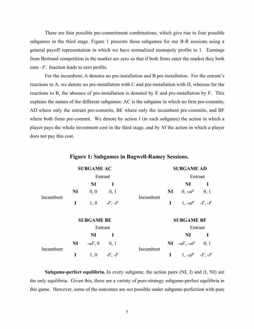
There are four possible pre-commitment combinations, which give rise to four possible

subgames in the third stage. Figure 1 presents these subgames for our B-R sessions using a

general payoff representation in which we have normalized monopoly profits to 1. Earnings

from Bertrand competition in the market are zero so that if both firms enter the market they both

earn –F. Inaction leads to zero profits.

For the incumbent, A denotes no pre-installation and B pre-installation. For the entrant’s

reactions to A, we denote no pre-installation with C and pre-installation with D, whereas for the

reactions to B, the absence of pre-installation is denoted by E and pre-installation by F. This

explains the names of the different subgames: AC is the subgame in which no firm pre-commits,

AD where only the entrant pre-commits, BE where only the incumbent pre-commits, and BF

where both firms pre-commit. We denote by action I (in each subgame) the action in which a

player pays the whole investment cost in the third stage, and by NI the action in which a player

does not pay this cost.

Figure 1: Subgames in Bagwell-Ramey Sessions.

SUBGAME AC SUBGAME AD

Entrant Entrant

NI I NI I

NI 0, 0 0, 1 NI 0, -aF 0, 1Incumbent Incumbent

I 1, 0 -F, -F I 1, -aF -F, -F

SUBGAME BE SUBGAME BF

Entrant Entrant

NI I NI I

NI -aF, 0 0, 1 NI -aF, -aF 0, 1Incumbent Incumbent

I 1, 0 -F, -F I 1, -aF -F, -F

Subgame-perfect equilibria. In every subgame, the action pairs (NI, I) and (I, NI) are

the only equilibria. Given this, there are a variety of pure-strategy subgame-perfect equilibria in

this game. However, some of the outcomes are not possible under subgame-perfection with pure

6

strategies. Any firm can guarantee itself zero profits by not pre-committing and then choosing NI

in all subgames; thus, no firm can obtain –aF in equilibrium. Also, since the pairs (NI, NI) and

(I, I) are not pure strategy equilibria in any subgame, the profit pairs (0, 0) and (-F, -F) cannot

occur as part of a subgame-perfect equilibrium.

But either of the two profit pairs (1,0) and (0,1) is consistent with subgame perfection.

For example, if both agents expect (NI, I) in all of the second-stage subgames, it is optimal for

the incumbent to not invest, and the entrant will be the monopolist (with or without pre-

commitment), with a profit of (0,1). The reverse holds if (I, NI) is expected in all of the second-

stage subgames, for a final profit of (1,0). Intuitively, if both firms believe that the incumbent

will be the winner in the second stage, this leads to an equilibrium where the incumbent is a

monopolist in the second stage and the entrant chooses to not pre-commit and stays out of the

market. The reverse happens if the firms believe that the entrant will ‘win’ after all first-stage

outcomes.

2.2. Forward Induction

Matters change under certain refined equilibrium notions of subgame perfection, which

select a unique equilibrium from the set. Kohlberg and Mertens (1986) introduced the concept of

‘forward induction’ with the aim of describing some desirable properties of an equilibrium

concept. In general terms, forward induction says that the actions of players have strategic

significance, and should be interpreted in this light. It can be described (Battigalli 1996) in the

following way: “A player should always try to interpret her information about the behavior of

her opponents assuming that they are not implementing ‘irrational’ strategies.”5 In our case the

forward-induction rationality requirements imposed by Bagwell and Ramey seem relatively

mild. Players should avoid weakly-dominated strategies, and their opponents should be aware of

this, and take it into account when making their decisions.6

5 Forward induction (as with other refined equilibrium concepts, like strategic stability) has, nevertheless, interestingconnections with bounded rationality. For a rich discussion of the concept and formal definitions, see Hauk andHurkens (2002).6 An alternative definition by Van Damme (1989, p. 485) states that when: “player i chooses between an outside

option or to play a game G of which a unique (viable) equilibrium *e yields this player more than the outside option,

only the outcome in which i chooses G and *e is played is plausible.” It is easy to see that this (stronger) notionyields the same result in this game.

7

Previous evidence on the predictive value of forward induction is rather mixed. Cooper,

DeJong, Forsythe & Ross (1992) analyze experiments involving a choice between an outside

option for one of the players and a 2x2 coordination game, with two Pareto-ranked equilibria.

They only analyze the case where forward induction and a simple dominance argument lead to

the same prediction. Their results are consistent with this kind of forward induction idea.

Cooper et al. (1993) present results from an experimental game, where there is an outside option

for one of the players and a symmetric Battle-of-the-Sexes game is played if this outside option

is foregone. When forward induction coincides with simple dominance the results are again

consistent with these notions. However, in a second treatment, an outside option that does not

dominate one of the other choices in the Battle-of-the-Sexes was observed to affect play in the

same manner as an outside option that does dominate.

Van Huyck et al. (1993) consider an experimental setting in which players participate in

an auction for the right to play a coordination game. Their results exhibit two key features: The

price in the auction is high enough for a forward induction argument (different from dominance

here) to select the Pareto-efficient equilibrium, and subjects’ play in the coordination game

actually selects this equilibrium. Schotter et al. (1994) study an experimental game for which the

application of iterated dominance selects one outcome and obtain results that are not consistent

with the predictions of the iterated dominance argument. The results presented in Brandts and

Holt (1995) do not support forward induction, except in a very simple game where it is

equivalent to the elimination of dominated strategies. Balkenborg (1998) reports results from a

game in which backward induction yields an outcome different from that resulting from forward

induction arguments; less than 20% of all cases result in the forward-induction outcome.

The focus in our paper is to consider forward induction in relation to a specific and

important issue in the area of industrial organization. For this purpose, we have learnt from

previous work and use experimental procedures that should give forward induction its best shot.

We give subjects considerable experience and put them in both the incumbent’s and the entrant’s

role to help them envision the strategic relations between the two firms.

In our game, forward induction gives the second mover an advantage. The argument

goes as follows: At the time of pre-commitment an entrant can guarantee himself a payoff of 0,

independently of what the incumbent has done, by not committing and then choosing NI. Thus,

any strategy under which a player pre-commits and then chooses NI is weakly dominated, as it

8

yields a lower payoff. Knowing that player 2 does not play dominated strategies, when player 1

observes a pre-commitment by player 2, he must conclude – according to the forward induction

logic - that player 2 intends to become the monopolist and will play I, and so player 1 will

respond optimally with NI.

As a consequence, player 2 will always (optimally) pre-commit, and then play I. In

contrast, pre-commitment does not have the same signaling value for the incumbent firm. An

incumbent that pre-committed could, mistakenly, have believed that the entrant was not going to

pre-commit (thus, expecting to become the monopolist). So, when faced with the unambiguous

subsequent pre-commitment choice of the entrant, the incumbent should yield and leave the

monopoly profits to the entrant. An incumbent who has not pre-committed has an even stronger

reason to yield in front of a pre-committed entrant. In anticipation of all this, the incumbent does

not pre-commit and leaves the market to the entrant.

Therefore, by forward induction, only the outcome (NI, I) is plausible. Taking this into

account, the first player will optimally respond by not pre-committing and then choosing NI in

all the subgames. So the set of strategies that survive the iterated deletion of weakly-dominated

strategies includes only the outcome (NI, I).

2.3. Iterated Deletion of Weakly-dominated Strategies.

In our experiments the game was played using the strategy-elicitation method.7 This

means that the incumbent had to choose whether to pre-install or not and also whether to

complete the investment or not for each of the entrant’s possible pre-installation decisions in the

second stage. Similarly, the entrant had to make a pre-installation decision for the incumbent’s

two possible pre-installation decisions, as well as a complete investment decision for the two

possible resulting pre-installation decisions of the two players.

The corresponding reduced normal form is shown in Table 1; it can be used to further

illustrate the selection rationale presented above. Here the incumbent is the row player and the

entrant the column player. The labels of the strategies are now those used in the experiment,

where the number “1” represents the choice of not completing the investment, NI, and the

number “2” means completing it, I. The reasoning we present holds for all positive values of a

7 This method allows the experimenter to collect data at every decision node. It can be considered to favor somewhatmore thoughtful behavior and is, hence, quite appropriate in this context.

9

and F. However, for ease of exposition, we now also use the same parameter values and payoffs

as in the experiment: We chose a = 1/2 and F = 1. We then transformed the payoffs by adding 1

to each payoff and then multiplying every payoff by 80. Thus, if both players choose I, each

receives 0. If only one player chooses I, he or she receives 160. Choosing NI gives a payoff of

80 without pre-installation; however, pre-installing and then choosing NI gives a payoff of 40.

Table 1: The Bagwell-Ramey game in reduced normal form.

CE11 E12 CE21 CE22 CF11 CF12 CF21 CF22 DE11 DE12 DE21 DE22 DF11 DF12 DF21 DF22

A11 80,80 80,80 80,160 80,160 80,80 80,80 80,160 80,160 80,40 80,40 80,160 80,160 80,40 80,40 80,160 80,160

A12 80,80 80,80 80,160 80,160 80,80 80,80 80,160 80,160 160,40 160,40 0,0 0,0 160,40 160,40 0,0 0,0

A21 160,80 160,30 0,0 0,0 160,80 160,80 0,0 0,0 80,40 80,40 80,160 80,160 80,40 80,40 80,160 80,160

A22 160,80 160,80 0,0 0,0 160,80 160,80 0,0 0,0 160,40 160,40 0,0 0,0 160,40 160,40 0,0 0,0

B11 40,80 40,160 40,80 40,160 40,40 40,160 40,40 40,160 40,80 40,160 40,80 40,160 40,40 40,160 40,40 40,160

B12 40,80 40,160 40,80 40,160 160,40 0,0 160,40 0,0 40,80 40,160 40,80 40,160 160,40 0,0 160,40 0,0

B21 160,80 0,0 160,80 0,0 40,40 40,160 40,40 40,160 160,80 0,0 160,80 0,0 40,40 40,160 40,40 40,160

B22 160,80 0,0 160,80 0,0 160,40 0,0 160,40 0,0 160,80 0,0 160,80 0,0 160,40 0,0 160,40 0,0

In this Table, the first (second) number after the last letter indicates whether I or NI was

chosen if the other person did not (did) choose to pre-install. So, for example, A12 means that

the incumbent did not pre-install, chose NI if the entrant did not pre-install and chose I if the

entrant did pre-install; DE21 means that the entrant pre-installed if the incumbent did not pre-

install, but did not pre-install if the incumbent did; in the third stage, the entrant chose I if the

incumbent did not pre-install and chose NI if the incumbent did pre-install.

First, notice that the incumbent has only one (strictly) dominated strategy: B11 (by A11).

This strategy consists of the incumbent pre-committing and then choosing NI in all the subgames

that can subsequently be reached. The fact that it is dominated simply means that it does not

10

make sense for a player to pre-commit if he does not want to become the monopolist (and so

obtain the (I, NI) outcome at some point). The entrant has one strictly-dominated strategy (DF11

by CE11), and several weakly-dominated strategies: CF11 (by CE11), CF21 (by CE21), DE11

(by CE11), DE12 (by CE12), DF12 (by CF12) and DF21 (by DE21). All of these dominated

strategies correspond to instances where the entrant pre-commits in some (or all) of the cases

when he can do so, and then chooses NI in the subgame(s) that follow(s) pre-commitment.

Once the weakly-dominated strategies of the entrant have been eliminated, the incumbent

has some weakly-dominated strategies: A12 (by A11), A22 (by A21), B12 (by A11) and B22 (by

B21). All of these strategies correspond to instances where the incumbent chooses I in a

subgame where the entrant has chosen to pre-commit. That can only be optimal if the entrant

chose NI in that subgame. However, such choices by the entrant are dominated, and have

already been eliminated.

The strategy DF22 for the entrant is now weakly dominant among the remaining

strategies. This strategy corresponds to the entrant always pre-committing and then choosing I in

all subgames. This is dominant because the (serially) undominated choice of the incumbent is to

play NI any time he ‘observes’ a pre-commitment by the entrant. Finally, since DF22 is

dominant, incumbent strategy B21 is sub-optimal, and the only strategies that remain for the

incumbent are A11 and A21. So the prediction is that the incumbent will not pre-commit, but

that the entrant will pre-commit and then become the monopolist.8

It is worth noticing that even without performing this last iteration (that is, with just two

rounds of deletion of dominated strategies), the entrant can guarantee his favorite outcome (NI,

I), as all the equilibria in the game that remains after two rounds of deletion produce that

outcome. In some of those equilibria the entrant does not even have to pre-commit. A less

stringent and perhaps more robust prediction would, therefore, be that the entrant becomes the

monopolist with or without pre-installation.

8 In general, the order of deletion of weakly dominated strategies might affect the final outcome of a given game.Not so in ours. The reason is that the strategies that are dominated (thus, eliminated) in (our) second round do notaffect the relationship between those that are dominated and dominant in (our) first round. For example, after justeliminating DE11, DE12, DF11 and DF12, we can eliminate A12 and A22. Even after this deletion CF11, CF21and DF21 are still weakly dominated by the same strategies we used.

11

2.4. The Dixit Game.

In our Dixit games, only the incumbent could pre-install, leading to only the two

subgames shown in Figure 2:

Figure 2: Subgames in Dixit Sessions.

SUBGAME A

EntrantNI I

NI 0, 0 0, 1Incumbent

I 1, 0 -F, -F

SUBGAME B

EntrantNI I

NI -aF, 0 0, 1Incumbent

I 1, 0 -F, -F

The forward-induction argument now points to the incumbent’s pre-installation decision.

The incumbent, at the time of pre-commitment can guarantee himself a payoff of 0,

independently of what the entrant does, by not committing and then choosing NI. As before, any

strategy under which a player pre-commits and then chooses NI is weakly-dominated, as it would

yield a lower payoff. Knowing that the incumbent does not play dominated strategies, when the

entrant observes a pre-commitment by the incumbent, he must conclude that the incumbent will

play I, and so responds optimally with NI. As a consequence, the incumbent will always

(optimally) pre-commit, and then play I. Therefore, by forward induction, only the outcome (I,

NI) is plausible. Taking this into account, the entrant will optimally respond by choosing NI in

the subgames. So the set of strategies that survive the iterated deletion of weakly dominated

strategies produces only the outcome (I, NI).

The corresponding reduced normal form is shown in Table 2, where, in the strategy

labels, the letters A and B refer to pre-installation decisions and the numbers have the natural

12

interpretation. We again chose a = 1/2 and F = 1, transforming the payoffs by adding 1 to each

payoff and then multiplying every payoff by 80.

Table 2: The Dixit game in reduced normal form.

11 12 21 22

A1 80,80 80,80 80,160 80,160

A2 160,80 160,80 0,0 0,0

B1 40,80 40,160 40,80 40,160

B2 160,80 0,0 160,80 0,0

Strategy B1, the incumbent pre-committing and then choosing NI, is strictly dominated

by strategy A1. With B1 eliminated, the entrant has two weakly-dominated strategies: 12 (by

11), and 22 (by 21). Once these have been eliminated, incumbent strategies A1 and A2 are

weakly dominated by B2. This strategy corresponds to the incumbent pre-committing and then

choosing I. So the prediction is that the incumbent will pre-commit and keep the market.

2.5. Experimental Design.

We conducted our sessions at Universitat Pompeu Fabra in Barcelona. Recruiting was

accomplished via announcements posted in university buildings; participants included students in

economics, business, law, political science, and the humanities. There were 12 (different) people

in each session; in fact there were two separate groups of six, although this was not mentioned.

This segmentation ensures two completely independent observations for each session. A session

consisted of 25 periods in which people were matched and randomly re-matched in pairs, within

the six-person subgroups. In addition, we alternated participants’ roles – if a person was a row

player (incumbent) in one period, he or she was a column player (entrant) in the next. We felt

that this alternation scheme offered the best chance for people to understand the subtleties

involved. The full instructions can be found in Appendix A.

13

We conducted six B-R sessions using the first of the two games described in the previous

section. Payoffs were re-normalized for experimental purposes, and are in pesetas (at the time,

$1 exchanged for approximately 180 pesetas). People received their earnings over 25 periods,

plus a show-up fee of 500 pesetas.

As already mentioned, in the B-R sessions play proceeded as follows: Each incumbent

stated whether he wished to pre-commit, and also stated a choice (I or NI) for each of the two

cases regarding possible pre-commitment by the entrant. Using the labels of the game above, the

incumbent had to choose between A and B, and to indicate his choice in the two possible

subgames that could result from the choice between A and B. Each entrant made choices

without being informed of the paired incumbent’s choices and stated whether she wished to pre-

commit if the incumbent had pre-committed and also whether she wished to pre-commit if the

incumbent had not pre-committed.9 Given her own pre-commitment choices, she also stated a

choice (I or NI) for each of the two cases regarding possible pre-commitment by the incumbent.

She had to indicate her choice both for A and for B, as well as her choices for the two possible

resulting subgames. After the data for the period was collected and matched up, each participant

was informed of his or her payoff outcome for that period.

As a control we also conducted three Dixit sessions. As in the B-R sessions, we had 25

periods with random re-matching. Here the incumbent stated his choice concerning pre-

commitment, as well as his choice (I or NI) in the resulting subgame. The entrant stated a choice

(I or NI) if the incumbent had pre-committed and also if the incumbent had not pre-committed.

So, overall, we had nine sessions, with a total of 108 participants. Average payoffs for the two-

hour sessions were around 2500 pesetas.

3. RESULTS

3.1. Realized Outcomes

We focus first on realized outcomes and move later to the consideration of strategy

choices to understand how outcomes eventuate.

9 We shall henceforth presume that the incumbent is male and the entrant is female, despite the fact that one’sgender must therefore change each period.

14

Table 3 shows the distribution of realized outcomes among the different cells of the B-R

game, separately for each of the twelve groups, where we now indicate whether the different

subgames involve P(reinstallation) or N(o) P(reinstallation) by the two players10:

Table 3: Realized Outcomes in the B-R Sessions.

Subgame AC (NP,NP) Subgame AD (NP,P)Group NI, NI NI, I I, NI I, I NI, NI NI, I I, NI I, I

1 13 13 13 10 0 5 1 52 10 5 20 10 1 6 0 33 3 3 22 14 0 14 1 64 5 1 7 5 1 2 0 35 9 8 29 22 0 0 1 26 6 3 22 18 0 3 1 77 8 3 41 7 0 1 1 58 13 2 49 10 0 0 1 09 8 5 11 6 2 13 1 710 5 0 31 8 1 1 1 811 6 12 11 17 0 5 1 312 5 9 5 5 2 8 1 9

91 64 261 132 7 58 10 58Aggregated

548 (60.9%) 133 (14.8%)

Subgame BE (P,NP) Subgame BF (P,P)Group NI, NI NI, I I, NI I, I NI, NI NI, I I, NI I, I

1 0 0 6 8 0 1 0 02 2 0 11 4 1 1 1 03 2 0 6 4 0 0 0 04 1 0 43 4 0 0 2 15 0 0 0 2 0 0 1 16 0 0 11 3 0 0 1 07 2 0 5 1 1 0 0 08 0 0 0 0 0 0 0 09 2 0 10 3 1 3 0 310 1 0 12 4 1 0 1 111 3 0 7 3 1 3 3 012 1 0 12 5 1 8 0 4

14 0 123 41 6 16 9 10Aggregated178 (19.8%) 41 (4.6%)

10 Recall that there were two completely independent six-person groups in each of our nine sessions.

15

Market capture and pre-commitment. In our context the most fundamental question is,

arguably, which of the two players captures the market. The answer represents the bottom line

with respect to the forward-induction prediction. If the entrant were to mostly become the

monopolist, this would, carried over to a wider context, imply that the incumbent would

somehow have to share the market with the entrant. We need to compare the sum of all (NI,I)

outcomes with that of all of the (I,NI) outcomes. The result is that the entrant becomes the

monopolist only 15% of the time, instead of the predicted 100%. By comparison, the incumbent

becomes the monopolist in 45% of the cases. Coordination failure is substantial with no one in

the market 13% of the time and both players in the market 27% of the time. Note, however, that

together this 40% is still below the rate of coordination on the incumbent becoming the

monopolist.

The natural next question is whether the incumbent’s preponderance is accomplished

through his pre-commitment. Overall, the incumbent pre-installs somewhat more often (24%)

than does the entrant (19%).11 When there is no pre-installation, the incumbent becomes the

monopolist 48% of the time (the corresponding figure for the entrant is 12%). When only the

incumbent pre-installs, he becomes the monopolist 69% of the time (the corresponding figure for

the entrant is 44%), so that pre-commitment does help the incumbent. Taken together these facts

allow us to say that the incumbent wins the market frequently and rather effortlessly, more so

than the entrant, in contrast to what theory suggests.

It is clear from Table 1 that there is a high degree of variance in behavior across groups.

For example, the group 4 incumbents took over the market in 55 (of 75) cases and the group 4

entrants took over the market in 3 cases, while for group 12 these figures were 18 and 25,

respectively. Pre-installation behavior also varied considerably by group. For example,

group 4 incumbents pre-installed 51 times, while group 8 incumbents never pre-installed; group

12 entrants pre-installed 33 times, while group 5 entrants pre-installed five times (and group 8

entrants pre-installed only once).

11 Incumbent pre-commitment results in subgames BE or BF (219 of 900 outcomes), while entrant pre-commitmentresults in subgames AD or BF (174 of 900 outcomes).

16

A high proportion of both entrants and incumbents chose to pre-install no more than 10%

of the time; however, there is considerable variation across the population. Comparing rates for

each individual in B-R, 35 individuals (of 72) were more likely to pre-install as an entrant than as

an incumbent, while this was reversed for 30 individuals; there was no difference in pre-

installation rates for seven participants. While few participants (19% of the incumbents and 3%

of the entrants) pre-installed more than half of the time in B-R, nearly 40% of the participants did

so (as the incumbent) in the Dixit sessions.

Comparisons across subgames. We now focus on different comparisons involving

observed frequencies in the different subgames, which we use to more clearly highlight the

degree of support for the general notion of pre-commitment as a tool for market control. We

start by observing that the incumbent’s pre-installation decision has only a very minor impact on

the entrant’s pre-installation rate: The entrant chooses to pre-install 18.7% of the time when the

incumbent pre-installs, compared to19.5% of the time when the incumbent does not pre-install.

At this point one might be tempted to jump to the conclusion that the strategic principles

put forward in game-theoretic analysis have no effect, even in its most basic form. Nevertheless,

pre-commitment by at least one firm occurs frequently enough in our data to warrant an

examination of how firms’ pre-commitment patterns and their relation to final investment (entry)

decisions affect subsequent choices. We next compare decisions within and across subgames,

and find that players’ decisions on whether to compete in the market are quite sensitive to pre-

installation choices of themselves and their counterparts.

Table 4 shows the proportion of eventual entry (choices of I strategies) into the market

for each player, contingent on pre-installation decisions. Focusing first on comparisons within

rows in the table, we observe the following pattern: When only one of the players pre-installs

that player completes the investment more frequently and, hence, can be thought of having an

advantage in capturing the market. When neither pre-installs the incumbent completes the

investment more frequently than the entrant; when both pre-install, the investment rate is

somewhat higher for the entrant.

12 In these Figures, each category on the horizontal axis shows the highest percentage. Thus, the first column meansthat nearly 50% of incumbents pre-installed between 0 and 10% of the time, inclusive. Rates for entrants areaggregated across whether or not the incumbent chose to pre-install.

17

Table 4: Market entry conditional on pre-installation (strategies).

Players pre-installing Incumbent’s investment % Entrant’s investment %

Incumbent only (BE) 92.1% 23.0%

Neither (AC) 71.7% 35.8%

Both (BF) 46.3% 63.4%

Only the entrant (AD) 51.1% 87.2%

Comparing the proportions along the columns, it is easy to see that a player is most likely

to invest when she alone has pre-installed and is much less likely to invest when only her

counterpart has pre-installed. Investment rates are at intermediate levels when neither player

pre-installs or when both players pre-install. Overall, aggregate choices of both first-mover and

second-mover (recall that all subjects are sometimes first-movers and sometimes second-movers)

were affected by pre-installation decisions. However, since the frequency of entrant pre-

installation is low, this sensitivity to pre-installation choices may just not be enough to yield the

Bagwell-Ramey predictions.

First-mover advantage. Some of the regularities that we have just discussed suggest that

there is a perceived first-mover advantage in this game. Observe the large difference in

investment rates (71.7% vs. 35.8%) when neither player pre-commits; in addition, note the

difference in these rates when only the other player has chosen to pre-install, 51.1% for the

incumbent compared to 23.0% for the entrant. In both cases, the investment rate for incumbents

is more than double the investment rate for entrants. Thus, while in the strategic analysis the

asymmetry of positions favors the entrant, in our data it appears to help the incumbent. It does

seem that there is a contingent of people who (correctly) believe that the second mover has the

advantage; this perception may prevail in groups 1, 11, and 12, for example.13 However, for the

majority of players the pattern is as if the incumbent had a ‘natural’ first-mover advantage,

something not captured by the strategic analysis presented above.

13 Note that the highest levels of ‘confusion’ are observed when only the second mover pre-installs, with an averageof 1.38 market participants. By contrast, the norms seem tightest (# of participants closest to the cooperative rate of1.00) when neither player pre-installs or when both players pre-install, with only 1.06 and 1.10 market participants,respectively.

18

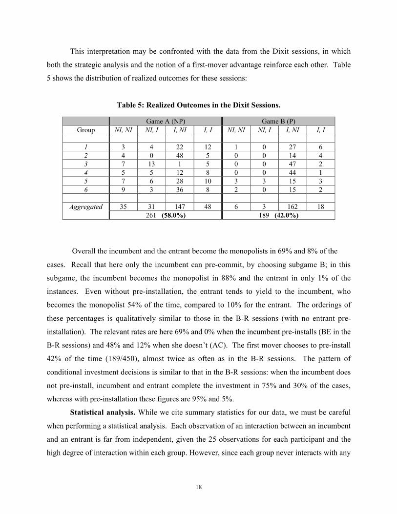
This interpretation may be confronted with the data from the Dixit sessions, in which

both the strategic analysis and the notion of a first-mover advantage reinforce each other. Table

5 shows the distribution of realized outcomes for these sessions:

Table 5: Realized Outcomes in the Dixit Sessions.

Game A (NP) Game B (P)Group NI, NI NI, I I, NI I, I NI, NI NI, I I, NI I, I

1 3 4 22 12 1 0 27 62 4 0 48 5 0 0 14 43 7 13 1 5 0 0 47 24 5 5 12 8 0 0 44 15 7 6 28 10 3 3 15 36 9 3 36 8 2 0 15 2

35 31 147 48 6 3 162 18Aggregated261 (58.0%) 189 (42.0%)

Overall the incumbent and the entrant become the monopolists in 69% and 8% of the

cases. Recall that here only the incumbent can pre-commit, by choosing subgame B; in this

subgame, the incumbent becomes the monopolist in 88% and the entrant in only 1% of the

instances. Even without pre-installation, the entrant tends to yield to the incumbent, who

becomes the monopolist 54% of the time, compared to 10% for the entrant. The orderings of

these percentages is qualitatively similar to those in the B-R sessions (with no entrant pre-

installation). The relevant rates are here 69% and 0% when the incumbent pre-installs (BE in the

B-R sessions) and 48% and 12% when she doesn’t (AC). The first mover chooses to pre-install

42% of the time (189/450), almost twice as often as in the B-R sessions. The pattern of

conditional investment decisions is similar to that in the B-R sessions: when the incumbent does

not pre-install, incumbent and entrant complete the investment in 75% and 30% of the cases,

whereas with pre-installation these figures are 95% and 5%.

Statistical analysis. While we cite summary statistics for our data, we must be careful

when performing a statistical analysis. Each observation of an interaction between an incumbent

and an entrant is far from independent, given the 25 observations for each participant and the

high degree of interaction within each group. However, since each group never interacts with any

19

other, one clean and conservative statistical approach is to consider only group-level data when

performing non-parametric tests.

Table 6 provides Wilcoxon signed-rank tests for a variety of comparisons. In all cases

the null hypothesis is the equality of the number of outcomes. For all instances for which we

indicate a prediction in the table the alternative hypothesis is the one that corresponds to the

direction of that prediction. In these cases we use one-tailed tests to reflect these ex ante

hypotheses. In the cases where we do not have a theoretical prediction, we use two-tailed tests:

Table 6: Non-parametric tests of Behavior across Subgames, by Group

B-R Sessions

Comparison of Rates Prediction Outcomes,by Group

p-value

Across Roles

IALL vs. EALL E > I 11I – 1E 0.998IAC vs. EAC - 9I – 2E 0.005*IAD vs. EAD E > I 8E – 2I 0.005IBE vs. EBE I > E 10I – 0E 0.001IBF vs. EBF E > I 3E – 4I 0.437PI vs. PE PE > PI 7I – 5E 0.765

Within Roles

IAC vs. IAD IAC > IAD 7AC – 5AD 0.170IAC vs. IBE IBE > IAC 9BE – 2AC 0.003IAC vs. IBF - 7AC – 3BF 0.348*IAD vs. IBE IBE > IAD 10BE – 1AD 0.002IAD vs. IBF IBF > IAD 5AD – 4BF 0.674IBE vs. IBF IBE > IBF 7BE – 1BF 0.008

IAC+AD vs. IBE+BF IBE+BF > IAC+AD 10B – 1A 0.007

EAC vs. EAD EAD > EAC 11AD – 1AC 0.001EAC vs. EBE EAC > EBE 8AC – 3BE 0.103EAC vs. EBF - 5AC – 3BF 0.547*EAD vs. EBE EAD > EBE 10AD – 1BE 0.001EAD vs. EBF EAD > EBF 8AD – 2BF 0.010EBE vs. EBF EBF > EBE 7BF – 3BE 0.138

EAC+AD vs. EBE+BF EAC+AD > EBE+BF 9A – 2B 0.009*Two-tailed test

20

Dixit Sessions

Comparison ofInvestment Rates

Prediction Outcomes,by Group

p-value

Across Roles

IALL vs. EALL I > E 6I – 0E 0.016IA vs. EA I > E 5I – 1E 0.047IB vs. EB I > E 6I – 0E 0.016

Within Roles

IA vs. IB IA < IB 6B – 0A 0.016EA vs. EB EA > EB 5A – 1B 0.078

In this Table, I and E refer to the respective investment rates for the incumbent and the entrant, and P refers to pre-commitment rates. Subscripts refer to subgames.

The comparison in the very first row, IALL vs. EALL, pertains to which of the two players

becomes the monopolist. The 11I-1E comparison means that the incumbent became the

monopolist more frequently (overall) than did the entrant in 11 of the 12 groups, providing very

little support for the alternative hypothesis. For all other across-role comparisons we compare,

for each group, the number of times that the incumbent invested vs. the number of times the

entrant invested. So, for example, the 9I-2E in the second row under Across Roles means that

the incumbent invested more frequently than did the entrant in 9 of 11 groups.

For within-role comparisons, we consider the incumbent and entrant investment rates for

each group. So, for example, the 9BE-2AC in the second row under Within Roles means that the

incumbents invested more frequently in subgame BE than in subgame AC for nine of 11 groups.

While we have data for 12 groups, there are often ties and/or cases where investment rates in a

category cannot be calculated (a zero divisor), so the number of comparisons is frequently less

than 12.

The tests confirm most of the descriptive analysis presented above. First, the group tests

confirm that the incumbent is significantly more likely to control the market in both the B-R and

the Dixit sessions. While this is in accord with the theoretical predictions when only the

incumbent can pre-install, it is not consistent with the predictions when the entrant has the final

pre-installation decision.

Nevertheless, the group tests also confirm that investment rates are highly sensitive to

pre-installation decisions. In the B-R game, while the incumbent is significantly more likely to

control the market when the entrant does not pre-install (subgames AC and BE), the entrant is

21

significantly more likely to control the market when she pre-installs and the incumbent does not

(subgame AD); there does not appear to be a consensus when both pre-install. Within-role

comparisons are particularly strong when they reflect a difference in the pre-installation decision

for that role, and no more than one party pre-installs, we see that IBE > IAC, IBE > IAD, EAC < EAD,

and EBE < EAD, all at easily significant levels. People clearly understand why they themselves

have pre-installed.

However, the effects are not as strong for within-role comparisons that reflect whether or

not the other party has pre-installed. Both the EBE vs. EAC and the IAC vs. IAD comparisons show

that there is some (not-quite-significant) tendency to respect the other firm’s pre-installation

choice. The only significant within-role comparisons involving the BF subgame are the cases

where the role player has pre-installed (IBE vs. IBF and EAD vs. EBF), suggesting that a player who

understands the logic of pre-installation is more likely to be sensitive to the pre-installation

decisions of others.

The group tests also confirm that the incumbent is significantly more likely to invest after

she has pre-installed than after she has not pre-installed (p = 0.007), and that the entrant is

significantly less likely to invest after the incumbent pre-installs (p = 0.009). However, there is

no significant difference in pre-commitment on a group basis.

In all six Dixit sessions, the incumbent invests more than the entrant when he has pre-

installed; without pre-installation, this still holds in five of the six sessions. Similarly, theincumbent invests more often in all sessions when he has pre-installed, while the entrant invests

less in five of the six sessions when the incumbent pre-installs.

3.2. Strategy Choices

Our results may look somewhat puzzling given the theoretical discussion in section 2.

After all, the solution via deletion of dominated strategies looks very sensible, given that only a

few rounds of elimination are necessary. One obvious explanation is that the rationality of

experimental subjects is lower than what is necessary for achieving the theoretical outcome. But,

one may wonder just how irrational these agents are. Up to now we have provided a rather

synthesized view of the results. Since we elicit full strategies for each player, we can also

examine the frequency of play for each strategy. The strategy choices as well as the

corresponding expected choice for each B-R session are shown in Table 7:

22

Table 7: Strategy Choices in B-R Sessions.

Complete 1st mover strategiesSession 1 2 3 4 5 6 7 8

A11 A12 A21 A22 B11 B12 B21 B22

1 42 7 41 25 1 1 11 222 22 2 18 45 3 0 4 563 20 7 26 78 0 1 3 154 21 6 33 81 2 0 5 25 22 13 29 44 1 3 16 226 33 13 26 27 0 5 26 20

Aggregate 160 48 173 300 7 10 65 137

Complete 2nd mover strategiesSession 1 2 3 4 5 6 7 8

CE11 CE12 CE21 CE22 CF11 CF12 CF21 CF22

1 53 9 19 32 2 2 1 42 66 3 16 20 1 0 2 03 63 13 21 31 1 2 2 14 106 12 9 13 2 0 0 05 59 4 16 5 2 12 3 66 33 6 29 10 1 4 11 8

Aggregate 380 47 110 111 9 20 19 19

Session 9 10 11 12 13 14 15 16DE11 DE12 DE21 DE22 DF11 DF12 DF21 DF22

1 1 1 14 4 1 0 3 42 4 0 13 5 1 0 1 183 0 1 7 2 1 0 3 24 1 0 2 1 0 1 3 05 2 0 18 5 2 2 4 106 2 1 8 8 0 4 3 22

Aggregate 10 3 62 25 5 7 17 56

To obtain a more in-depth view of subjects’ behavior we need to look at the expected ex

post payoffs of complete strategy choices, as well as the frequency of these choices. Table 8

displays this information, where strategies have been ordered by the frequency of their choice.

Using the information in Tables 7 and 8 we can now discuss incumbents’ and entrants’ strategy

23

choices and afterwards move to an analysis of why the iterated elimination of dominated

strategies does not fully work in our experiment.

Table 8: Ex post Expected Earnings for each Strategy

Bagwell-Ramey SessionsIncumbent Strategies Entrant Strategies

Strategy Frequency Exp. Earnings Strategy Frequency Exp. EarningsA22 .333 85.5 CE11 .422 80.0A21 .192 97.5 CE22 .123 40.0A11 .178 80.0 CE21 .122 56.4B22 .152 108.8 DE21 .069 78.7B21 .072 100.3 DF22 .062 72.0A12 .053 68.0 CE12 .052 63.6B12 .011 40.0 DE22 .028 62.2B11* .008 40.0 CF12 .022 73.3

CF22 .021 49.8CF21* .021 46.7DF21* .019 68.9DE11* .011 49.7CF11* .010 70.3DF12* .008 43.1DF11* .006 40.0DE12* .003 33.3

*Indicates that a strategy is at least weakly dominated in the first round of iterations.

Incumbent strategies. Tables 7 and 8 reveal that the predicted strategies are not the most

frequently chosen ones and that neither the predicted ones nor the most frequent ones are the

most profitable ones. Recall that the two incumbent strategies that should be played according to

forward induction are A11 and A21. However, the most commonly-used incumbent strategy

(33.3%, by far the highest) is A22 (do not pre-install and always invest later). Strategy B22 is

used roughly as often as the predicted ones.

A22 has an expected ex post payoff of 85.5, better than the safe payoff of 80 that is

available by not pre-installing and never investing (A11). Choosing A22 could indicate that the

incumbent thinks that it is likely that the second player thinks that the first mover has the

advantage. However, the first mover could increase own payoffs by either choosing A21, which

only differs from A22 in that the incumbent chooses not to complete the investment if he

observes pre-installation by the second player. He would earn even more by just pre-installing

24

and playing B21 or, even better, B22 (so certainly play I if the second player does not pre-

install). Pre-installing really clears the way for the incumbent’s market dominance here.

A11 is chosen almost 18% of the time. This strategy is supported in the B-R equilibrium.

A21 is like A11 except that it chooses I if player 2 does not pre-install. It does better than the

more aggressive A22 strategy, as the expected payoff from playing I in AD is only 21.6,

compared to 80 for NI. In fact, many people follow these incentives – A21 is played 19% of the

time, and does best of all the no-pre-installation strategies.

The most profitable strategy, B22, is chosen 137/900 or 15.2% of the time. Perhaps its

frequency could increase over time. The number of times it is chosen (grouped in ascending 5-

period intervals) is 20, 26, 27, 30, and 34, so that it is gradually growing in frequency; the 34

B22 choices in the last five periods represents close to 20% of all choices in the final five

periods. B21 is like B22 except that it chooses NI if the second player pre-installs. It is chosen

65/900, or 7% of the times. It has a reasonable expected payoff, 100.3, and its frequency seems

‘stable’ over time, with aggregate choices being 15, 9, 13, 14, and 13.

A12, B11, and B12 are played with such low frequencies, combined 65/900 or 7%, that

one may view them as errors or experiments. Perhaps reassuringly, the only directly-dominated

choice, B11, is the least used one.

Entrant strategies. The most common entrant strategy, used in 42.2% of the cases, is

CE11, which consists of never pre-installing, then always playing NI and, hence, staying out of

the market. It was chosen more than three times as frequently as any other strategy, and in fact

this strategy pays the best ex post against the observed aggregate first-mover strategy. It is also

the completely safe strategy, with a guaranteed payoff of 80. Looking at both players at the

same time, the most frequent strategy combination is the one where the incumbent does not pre-

commit and goes for the market regardless of the entrant’s behavior and where the entrant never

pre-installs and yields the market, regardless of what the incumbent does.

The next most common entrant strategies are CE21 and CE22 (110/900 or 12.2%,

111/900 or 12.3% respectively). CE21 prescribes the following: Do not pre-install, choose I if

the first-mover does not pre-install, but choose NI if he does. CE21 does not do well, getting an

expected payoff of 56.4, since only 208/900 of the incumbents who do not pre-install yield in

subgame AC. This is even worse with CE22 (the same as CE21, except that it plays NI against a

25

pre-committed incumbent), yielding 40.0.14 How do they do these strategies do over time? The

5-period frequencies for CE21 are 25, 16, 23, 22, and 24. Regarding CE22 over time, the 5-

period frequencies are 31, 27, 18, 18, and 17. There is no obvious trend in the first case, while

the latter appears to be a downward trend.

DF22 is the prediction under the iterated elimination of weakly-dominated strategies;

always pre-install and play NI in the subgames that follow. This is optimal provided that the first

mover chooses NI in all subgames. It happens very infrequently, 56/900 or 6.2% of the time.

This strategy has an ex post expected payoff of 72, given the observed distribution of first-mover

strategies

DE21 is the strategy where the second mover pre-installs if and only if the first mover

doesn’t. It then chooses I, if the first mover does not install, and NI when the first mover pre-

installs. This strategy is chosen 62/900 or 6.9%. It does almost as well as the completely safe

strategy of CE11, and becomes somewhat more popular over time – the 5-period frequencies are

5, 16, 10, 16, and 15.

The strategies that start with CF represent a pre-installation as a second mover only if the

first mover has pre-installed. They collectively happen only 67/900 times or 7.4% of the time.

The strategies DE11, DE12, DE22, DF11, and DF12 account for a total of 50/900 or 5.6%.

None of these strategies are very profitable.

Why does the iterated elimination not work? Recall that the only dominated strategy

for player 1 is B11. For player 2, the strategies that are dominated in the first round are CF11,

CF21, DE11, DE12, DF11, DF12, and DF21. None one of these are played very often. The

highest frequency is 19/900; collectively this is 70/900, which is still quite low, particularly

when taking into consideration that they might have been used to test the response of player 1 to

different modes of pre-commitment.

So one could argue that subjects do largely avoid weakly-dominated strategies. But,

crucially for the lack of empirical success of the B-R predictions, the subsequent round of

deletion fares much more poorly in the data. The first and the fourth most used strategies for

player 1 are A22 and B22 (frequencies 300/900 and 137/900), which are dominated if the first

14 Note that CE22 is the strategy chosen by entrants who believe that the entrant has an advantage and should noteven have to pre-install to capture the market. It is the complement to incumbent strategy A22, where the incumbentis always aggressive but doesn’t pre-install, apparently perceiving a first-mover advantage. CE22 was chosen 111times, compared to 300 times for A22.

26

round of deletion goes through. So given that those strategies dominated in the first round are

used so rarely, how do these relatively common other strategies survive? The answer is that the

strategies for player 2 that make this domination apparent are also quite infrequent.

To make this discussion more concrete, take as an example B22, which is dominated (in

the second round) by B21. The payoffs of these two strategies of player 1 differ only against the

following strategies for player 2: CF11, CF12, CF21, CF22, DF11, DF12, DF21 and DF22. B22

does worse than B21 when paired with CF12, CF22, DF12, and DF22, and does better when

paired with the other ones: CF11, CF21, DF11, and DF21. But CF11, CF21, DF11, and DF21

are all weakly dominated, which is why B22 disappears under iterated deletion. However, in

practice the frequencies of these eight strategies for player 2 are all quite small, so the payoffs of

both B22 and B21 are quite similar, even at the aggregate level, and given the individual

uncertainty are probably indistinguishable for most players. Moreover, the frequency of CF12,

CF22, DF12, and DF22 must collectively be at least three times greater than that of CF11, CF21,

DF11, and DF21, in order for the expected payoff of B21 to even be larger than that of B22.

And this is not the case, so in fact the expected aggregate payoff of B22 is a bit better that that of

B21. Again, this is all aggregated data; at the individual level, the difference must be difficult to

discern.

Something similar happens when looking at A22, which is dominated (in the second

round) by A21. The only difference is that in this case, the aggregate payoff is somewhat higher

for A21. But once again the differences are modest, so that at the individual level they are

swamped by the uncertainty. So this can explain why strategies that are dominated in the second

round do not disappear. After that the third round of deletion would not be optimal.

Hence, a pre-conception, like the notion of the first mover having an advantage can

completely stall the progress of iterated deletion. But even if agents are (mildly) boundedly

rational, it may be possible for them to learn to avoid dominated strategies via the repeated

interaction. In the next section we will show that this argument is misleading.

4. DYNAMICS AND SIMULATIONS

We mentioned earlier that it is now widely recognized that learning by boundedly

rational agents does not necessarily eliminate weakly dominated strategies. As the intuitive

27

arguments suggest, under learning or evolution a strategy that does worse than another one will

tend to be observed less frequently. But if the strategy against which the dominated strategy

does poorly is also decreasing over time (so that the advantage of the dominating one becomes

smaller as well), the decrease of the dominated strategy will be slower and slower, so that it can

stabilize at a positive level.

We will now show, first with a theoretical framework for deterministic dynamics, and

then through simulation under stochastic dynamics, that the equilibria with iteratively dominated

strategies can survive in the long run under learning in this game, and that models of learning can

track observed behavior in the lab reasonably well. The analytical and simulation results are

complementary. The analytical results with deterministic dynamics are rather general (within

their class) but only suggest a possibility, namely, that given the “right” initial conditions,

iteratively weakly dominated strategies may survive in the limit as time goes to infinity.15 The

simulations show that even in small populations, with a short time-horizon, particular stochastic

learning models have many of the features of our data, in particular that iteratively weakly

dominated strategies can survive for the duration of our experiment.

Deterministic dynamics. We must first introduce some notation: Let isix be the

probability assigned by the player i to strategy is . Let iix DΠbe a mixed strategy for agent i,

where iD is the simplex which describes player i’s mixed-strategy space. We formalize the

behavior of each player in terms of the mixed strategy he adopts at each point in time, so the

vector ))(),(()( 21 txtxtx = will describe the state of the system at time t,16 defined over the

simplex 21 D¥D=D of which 0D is the relative interior.

Assumption d.1. The evolution of x(t) is given by a system of continuous-time differential

equations:

)).(()( txDtx ii si

si =

15 Deterministic dynamics can (and perhaps should) be interpreted as limits of stochastic dynamics for largepopulations (Cabrales 2000) or for slow adaptation (Börgers and Sarin 1997).

28

We require that the autonomous system satisfies the standard regularity conditions; i.e. D must

be (i) Lipschitz continuous with (ii) .0))(( =S ΠtxD i

ii

siSs Furthermore, D must also satisfy the

following requirements:

Assumption d.2. D is a regular (payoff) monotonic selection dynamic. More explicitly, let

)(/)())(,( txtxtxsg ii si

siii &≡ denote the growth rate of strategy is . Then, for all is , 'is and all

)(tx , it must be true that

[ ] [ ]))(,'())(,())(,'())(,( txsutxsusigntxsgtxsgsign iiiiiiii -=- .

Assumption d.2 merely says that a strategy that has a higher payoff, given the current state of the

population grows faster (decreases more slowly) than a strategy with a lower payoff.

Assumption d.3. 0)0( DŒx .

This assumption is a technical necessity because regular dynamics are such that a strategy with

zero initial weight will have zero weight at all subsequent times. So a weakly-dominant strategy

will have no power against dominated ones, when the strategies of other players against which it

does well are never used. This assumption guarantees that the survival of dominated strategies

does not arise simply due to an initial non-existence of those strategies.

We will now show that the elements in one of the subgame-perfect equilibrium

components which does not survive iterated deletion are limit points of the dynamics from some

interior solution. To state the theorem we introduce more notation. By Lipschitz continuity

there is a constant ,0>K such that, for all iii xxs -- ',, we have that:

iiiiiiii xxKxsgxsg ---- -£- ')',(),(

where the

†

. denotes the norm of a vector. This in turn implies that when

1),'(),( -<- -- iiiiii xsuxsu , there exists some h such that hxsgxsg iiiiii -£- -- )',(),( .

16 As is common in the evolutionary literature ( x(t), y(t)) can also be interpreted as the proportions of people playingeach strategy when a game is repeatedly played by a randomly-matched large population.

29

Proposition 1. Assume that

†

2 Kh

1-x2

si (0)x2

CE11(0)si œS2*

Â

Maxsi ≠CE12* x2

si (0)x2

CE12(0) >9

16 and that

†

2 Kh

1-x1

si (0)x1

A22 (0)siœ A 21, A 22{ }

Â

MaxsiΠA21, A22{ }x1si (0)

x1A22 (0) >

78

(a) For all

†

si œ CE11,CE12,CF11,CF12{ } , and for all t,

†

x2si (t) < exp(-ht ) x2

si (0)x2

CE11(0)

(b) For all t, .16

9)(21

2 >tx ZCES

(c) For all

†

i œ A21,A22{ } , and for all t,

†

x1si (t) < exp(-ht ) x1

si (0)x1

A22(0)

(d) For all t,

†

x1A22 (t ) >

78

.

Proof: See Appendix B.

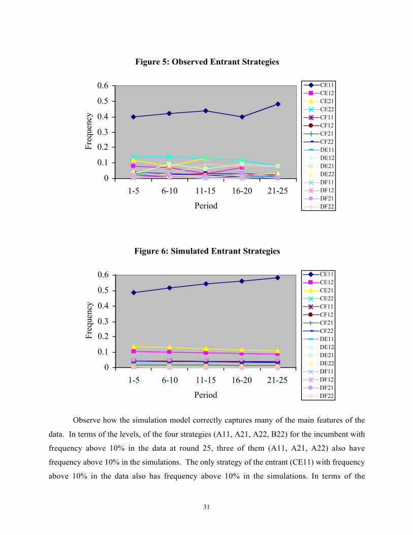
Simulation results. We next present simulation results based on the Camerer and Ho (1999)

learning model. Figures 3 and 4 show in parallel the observed and predicted frequencies of use

for the eight different incumbent strategies, while Figures 5 and 6 show observed and

frequencies of use for the 16 different entrant strategies. The graphs show the average of 1000

simulation runs.17

17 We chose the following parameter values: phi= 0.9 and lambda=1.2.

30

Figure 3: Observed Incumbent Strategies

0

0.1

0.2

0.3

0.4

0.5

1-5 6-10 11-15 16-20 21-25

Period

Freq

uenc

yA11A12A21A22B11B12B21B22

Figure 4: Simulated Incumbent Strategies

0

0.1

0.2

0.3

0.4

0.5

1-5 6-10 11-15 16-20 21-25

Period

Freq

uenc

y

A11A12A21A22B11B12B21B22

31

Figure 5: Observed Entrant Strategies

0

0.1

0.2

0.3

0.4

0.5

0.6

1-5 6-10 11-15 16-20 21-25

Period

Freq

uenc

yCE11CE12CE21CE22CF11CF12CF21CF22DE11DE12DE21DE22DF11DF12DF21DF22

Figure 6: Simulated Entrant Strategies

0

0.1

0.2

0.3

0.4

0.5

0.6

1-5 6-10 11-15 16-20 21-25

Period

Freq

uenc

y

CE11CE12CE21CE22CF11CF12CF21CF22DE11DE12DE21DE22DF11DF12DF21DF22

Observe how the simulation model correctly captures many of the main features of the

data. In terms of the levels, of the four strategies (A11, A21, A22, B22) for the incumbent with

frequency above 10% in the data at round 25, three of them (A11, A21, A22) also have

frequency above 10% in the simulations. The only strategy of the entrant (CE11) with frequency

above 10% in the data also has frequency above 10% in the simulations. In terms of the

32

dynamics, notice, for example, that the general trends of A11 (moderately downwards) and A22

(slightly upwards) are well captured. The simulations also capture the moderate upward trend

for the entrant’s strategy CE11. We also wish to highlight that, consistent with the intuitive

argument presented above, B21 does not grow at the expense of B22. Similarly A21 does not

grow at the expense of A22.

5. CONCLUSION

There is a puzzle in industrial organization: Despite the theoretical arguments advanced

for entry deterrence by incumbents, there is little empirical evidence that firms behave in this

manner. Bagwell and Ramey (1996) propose an alternative model of the timing in the entry

game, providing a ‘last-mover advantage’ through the logic of forward induction. It is suggested

that this is the reason that incumbent firms do not engage in entry deterrence.

We study behavior in a simplified version of the B-R model and compare it to

observations from the simpler Dixit game. Our work is, hence, an experimental investigation of

a theoretical rationalization of field evidence. We find that in both games the first mover tends

to capture the market. This does not require a strong propensity towards pre-commitment by the

first mover in either case, although a strong minority of incumbents do engage in frequent pre-

installation in the Dixit game. Nevertheless, pre-commitment by the incumbent helps

profitability.

In the B-R game, the strategy in which the incumbent does not pre-install, but

nevertheless enters the market regardless of the entrant’s pre-installation decision, is by far the

most common (chosen fully 1/3 of the time). The logic of forward induction makes some

inroads against an a priori perception of a first-mover advantage, but generally must surrender to

it – the strategy leading to the highest expected payoff for an entrant in the B-R game involves

always staying out of the market. On the other hand, forward induction and such a perception

work together in the Dixit game, and the incumbent enjoys an overwhelming advantage.

Just to posit the existence of a perceived first-mover advantage is not a sufficient

explanation of our data; one must also clarify why learning does not do away with this pre-

conception. Our theoretical result with deterministic dynamics and our stochastic simulation

33

model results provide a rationale for why the initial behavior does not change too much over

time.

Thus we feel that we have obtained a rather complete explanation of why forward

induction is only weakly supported in our data. It is not simply based on the notion that people

have limitations in their depth of reasoning. Rather, matters start with a pre-conception that

subsequent experience with the environment is unable to erase.

One may wonder about the origins of a perceived first-mover advantage. Our result bears

relation to some recent experimental findings reported in Weber and Camerer (2002) and Muller

and Sadanand (2003). These studies show that when simple two-person games that are

‘simultaneous’ in terms of information are played sequentially, the first mover tends to do better

than when both players make actual simultaneous choices. Note that this cannot be explained

just by the fact that the temporal asymmetry in moves allows for better coordination and that

players use any available clue to facilitate coordination. If this were the driving force, then a

second player advantage could arise just as well. There appears to be something special about

moving first.

Huck and Müller (2000) report another instance of a first-mover advantage that

transcends game-theoretic prediction. They study experimentally the Bagwell (1995) result that

the commitment value of moving first is severely undermined if the observability of the earlier

move is even slightly in doubt and find that people do not ignore prior moves even with

imperfect observability.

Our environment is somewhat different since the second mover does observe (at least in

principle) the first mover’s choice. However, perhaps there is something more general in the

psychology of reasoning about timing that favors earlier movers. Weber and Camerer (2002)

suggest that, consistent with some evidence from psychological experiments, players may be

better at reasoning backward, about events known to have already happened, than reasoning

forward. Description of possible outcomes of previously-occurring events is often richer and

more complex than description of later-occurring events. Weber and Camerer conjecture on p.29

that “the past is easier to ‘imagine’ than the future.”

What can we say about the excess capacity puzzle that brought us here? While our

evidence does not support the B-R prediction, it suggests, perhaps paradoxically, that the B-R

environment may be the better one to study the matter at hand. Both firms have an opportunity

34

for capacity investment but neither uses it very much, resulting in a prevailing tendency of

market dominance by the incumbent.

REFERENCES

Bagwell, K. (1995), “Commitment and Observability in Games,” Games and EconomicBehavior, 8, 271-280.

Bagwell, K., and G. Ramey (1996), “Capacity, Entry and Forward Induction,” RAND Journal ofEconomics, 27, 660-680.

Bain, J. (1956), Barriers to New Competition, Cambridge, MA: Harvard University Press.Balkenborg, D. (1998), “An Experiment on Forward- versus Backward Induction,” University of

Southampton, mimeo.Battigalli. P. (1996), “Strategic Rationality Orderings and the Best Rationalization Principle,”

Games and Economic Behavior, 13, 178-200.Basu, K. (1993), “Lectures in Industrial organization Theory,” Blackwell Publishers: Oxford,

UK.Börgers, T. and R. Sarin (1997), “Learning Through Reinforcement and Replicator Dynamics,”

Journal of Economic Theory, 77, 1-14.Brandts, J. and C. Holt (1995), “Limitations of dominance and forward induction: Experimental

evidence”, Economics Letters, 49, 391-395.Cabrales, A. (2000), “Stochastic Replicator Dynamics,” International Economic Review, 41,

451-481.Camerer, C. and T. Ho (1999), “Experience-Weighted Attraction in Games,” Econometrica, 67,

827-874.Cooper, R., D. DeJong, R. Forsythe and T. Ross (1992), “Forward induction in coordination

games”, Economics Letters, 40, 167-172.Cooper, R., D. DeJong, R. Forsythe and T. Ross (1992), “Forward induction in the battle-of-the-

sexes games”, American Economic Review, 83, 1303-1316.Dixit, A. (1980), “The Role of Investment in Entry Deterrence,” Economic Journal, 90, 95-106.Fudenberg, D. and D. Levine (1998), The Theory of Learning in Games, MIT Press, Cambridge

MA.Geroski, P. (1995), “What do we Know about Entry?” International Journal of Industrial

Organization, 13, 421-440.Hauk, E. and S. Hurkens (2002), “On Forward Induction and Evolutionary and Strategic

Stability,” Journal of Economic Theory, 106, 66-90.Huck, S. and W. Müller (2000), “Perfect versus imperfect observability – An experimental test

of Bagwell’s result”, Games and Economic Behavior, 31, 174-190.Kohlberg, E. and J.-F. Mertens (1986), “On the Strategic Stability of Equilibrium,”

Econometrica, 54, 1003-1038.Martin, Stephen (1993), Advanced Industrial Economics, Basil Blackwell.Mason, C.F. and C. Nowell (1998), “An experimental analysis of subgame perfect play: the entry

deterrence game,” Journal of Economic Behavior and Organization, 37, 443-462.

35

Modigliani, F. (1958), “New developments on the oligopoly front”, Journal of PoliticalEconomy, 66, 215-232.

Muller, R. and A. Sadanand (2003), “Order of Play, Forward Induction, and Presentation Effectsin Two-Person Games”, Experimental Economics, 6, 5-25.

Samuelson, L. (1997), Evolutionary Games and Equilibrium Selection, MIT Press: CambridgeMA.

Schotter, A., K. Weigelt and C. Wilson (1994), “ A laboratory investigation of multipersonrationality and presentation effects,” Games and Economic Behavior, 6, 445-468.

Singh, S., M. Utton and M. Waterson (1998), “Strategic Behavior of Incumbent Firms in theU.K.,” International Journal of Industrial Organization, 16, 229-251.

Smiley, R. (1988), “Empirical Evidence on Strategic Entry Deterrence,” International Journal ofIndustrial Organization, 6, 167-180.

Tirole, J. (1989), The Theory of Industrial Organization, MIT Press: Cambridge MA.Van Damme, E. (1989), “Stable Equilibria and Forward Induction,” Journal of Economic

Theory, 48, 476-496.Van Huyck, J., R. Battalio and R. Beil (1993), “Asset markets as an equilibrium selection

mechanism: Coordination failure, game form auctions, and tacit communication,” Gamesand Economic Behavior, 5, 485-504.

Vives, X. (1999), Oligopoly Pricing: Old Ideas and New Tools, MIT Press: Cambridge MA.Vega-Redondo, F. (1996), Evolution, Games and Economic Behavior, Oxford University Press:

Oxford, UK.Weber, R. and C. Camerer (2002), “Timing and Observability in Ultimatum Games and ‘Weak

Link’ Coordination Games,” mimeo.

36

APPENDIX A - INSTRUCTIONS

Thank you for participating in this experiment. For your participation you will receive a positive amount ofmoney. This quantity will be determined by the way in which your decisions relate to those of the other players. Youwill, in any case, receive 500 pesetas, that is in addition to the amount of money you make during the experiment.

In this experiment there will be 25 rounds. In each round you will be paired with a different person in theroom. You will not be informed about the identity of the person that you are paired with in any of the rounds, neitherduring the experiment nor afterwards. Neither will anybody know that they are or have been paired with you at anymoment.

In each round there will be a Player 1 and a Player 2. The players determine which game is played in eachround. Whether you are Player 1 or Player 2 will be determined randomly in each round, so that you will bealmost for sure in each of the roles at some point in the session. Player 1 decides whehterh she chooses action A oraction B. Player 2 chooses action C or action D for the case where Player 1 has chosen A, and action E or action Ffor the case where Player 1 has chosen B.

For the case in which Player 1 has chosen action A, and Player 2 has chosen C for the case in which 1 chooses A,the relevant game is AC.For the case in which Player 1 has chosen action A, and Player 2 has chosen D for the case in which 1 chooses A,the relevant game is AD.For the case in which Player 1 has chosen action B, and Player 2 has chosen E for the case in which 1 chooses B, therelevant game is BE.For the case in which Player 1 has chosen action B, and Player 2 has chosen F for the case in which 1 chooses B, therelevant game is BF

All the payoffs you can see in the tables are in pesetas; the first of the two numbers that can be seen in acellcorresponds to the payoff for Player 1 and the second number corresponds to the payoff for Player 2.

GAME AC GAME AD

Player 2 Player 2

S1 S2 U1 U2

R1 60,60 60,120 T1 60,30 60,120

Playerr 1 Player 1

R2 120,60 0,0 T2 120,30 0,0

GAME BE GAME BF

Player 2 Player 2

Z1 Z2 Y1 Y2

W1 30,60 30,120 X1 30,30 30,120

Player 1 Player 1

W2 120,60 0,0 X2 120,30 0,0

37

.APPENDIX B – PROOFS

Proof of Proposition 1: Suppose that (a) is the statement that stops being true the earliest, that it

does so for strategy is and that the boundary time is t’. Then it must be that:

†

x2si (t ') = exp(-ht ') x2

si (0)x2

CE12(0).

Note that

†

u2 (si , x1) £ 4x1A22

+16(1- x1A22 ) £11/ 2 , and also that

†

u2 (CE12, x1) ≥ 8(x1A12

+ x1A22 ) ≥ 7 , where the last inequality in both cases, holds because by (d)

and the assumption here for all t < t’,

†

x1A22 (t ) ≥ 7 /8.

Thus,

†

u2 (si , x1(t)) -u2 (CE12,x1 (t)) < -1, so by continuity and assumption d.2 there exists

)(ah such that

†

gi (si ,x1(t ))- gi(CE12, x1(t)) < -h for all t<t’. Then, by integrating, we have that

†

x2si (t ' )

x2CE 12(t' )

< exp(-ht' ) x2si (0)

x2CE 12(0)

, which implies

†

x2si (t ') < exp(-ht ') x2

si (0)x2

CE12(0)x2

CE12(t ' ) £ exp(-ht ') x2si (0)

x2CE12(0)

, a contradiction.

Suppose, then, that (b) is the statement that stops being true the earliest, that it does so for

strategy is and that the boundary time is t’. Then it must be that: .16

9)(21

2 =tx ZCES As before, we

will reach a contradiction, but before we will prove the following:

Claim: For all

†

si ΠCE11,CF11,CF12{ }

))()(1(2))(,())(,( 2221

111121 txtxKtxsgtxZCESg TARTARiii ---≥- .

Proof of Claim: For all

†

si ΠCE11,CF11,CF12{ } , since

†

u2 (si , ˆ x 1)) = u2 (CE12, ˆ x 1 ),for all 1̂x such

that

†

ˆ x 1A21

+ ˆ x 1A22

=1, we have that

†

gi (CE12, ˆ x 1 (t )) = gi(si , ˆ x 1(t)) . So, by Lipschitz-continuity we

have that for all 1x

†

gi (CE12,x1 (t ))- gi(CE12, ˆ x 1(t)) ≥ -2K x1(t) - ˆ x 1(t)

38

)(ˆ)(2))(,())(ˆ,( 1111 txtxKtxsgtxsg iiii --≥-

But since

†

gi (CE12, ˆ x 1 (t )) = gi(si , ˆ x 1(t)) , adding the previous two inequalities yields the result.�

Now, by the claim,

†

gi (CE12,x1 (t ))- gi(si , x1(t)) ≥ -2K (1- x1A12(t) - x1

A22 (t)) , but by

assumption, for all t<t’

†

x1si (t) < exp(-h(c)t)

x1si (0)

x1A22(0)

for all

†

si œ A21, A22{ } so that

†

gi (CE12,x1 (t ))- gi(si , x1(t)) ≥ -2K (exp(-h(c)t)x1

si (0)si œ A21,A 22{ }

Â

x1A22 (0)

) . Then by integration we have that

†

x2CE 12(t ')

x2CE12(0)

x2si (0)

x2si (t ')

> 2 Kh(c)

x1si (0)

si œ A21,A 22{ }Â

x1A22 (0)

≥ 2 Kh(c)

. This implies that

†

x2CE 12(t ')

x2CE12(0)

> 2 Kh(c)

x2si (t ')

x2si (0)

and by summing over all

†

si ΠS2*

≡ CES1Z1,CE12,CF11,CF12{ } we have that:

†

x2CE 12(t ')

x2CE12(0)

> 2 Kh

x2si (t ')

si ŒS2*

Â

Maxsi ΠS2

* x2si (0)

= 2 Kh

1- x2si (t ')

si œS2*

Â

x2si (0)

≥ 2 Kh

1-x2

si (0)x2

CE 12(0)si œS2*

Â

Maxsi ΠS2

* x2si (0)

where the last inequality is true by (a). This yields a contradiction by the assumption about the

initial conditions.

Suppose that (c) is the statement that stops being true the earliest, that it does so for strategy

is and that the boundary time is t’. Then it must be that:

†

x1si (t ') = exp(-h(c)t ')

x1si (0)

x1A22(0)

.

Note that

†

u1(si , x1) £16(1- x2CF12 ) £ 7 and also that

†

u1(A22, x1) ≥16x2CF12

≥ 9 , where the last

inequality in both cases, holds because by (d) and the assumption here for all t < t’,

†

x1CF 22(t ) ≥ 9/16.

39

Thus,

†

u1(si , x2 (t)) -u1 (A22, x2 (t)) < -1, so by continuity and assumption d.2 there exists )(ah such

that

†

gi (si ,x2(t ))- gi(A22, x2(t )) <-h(a) for all t<t’. Then, by integrating, we have that

†

x1si (t ' )

x1A22 (t ')

< exp(-ht' ) x1si (0)

x1A22 (0)

, which implies

†

x1si (t ') < exp(-ht ') x1

si (0)x1

A22(0)x1

A22(t ') £ exp(-ht ' ) x1si (0)

x1A22 (0)

, a contradiction.

Suppose, then, that (d) is the statement that stops being true the earliest, that it does so for

strategy is and that the boundary time is t’. Then it must be that:

†

x1A22 (t ') = 9/16. As before, we will reach a contradiction, but before we will prove the

following:

Claim:

†

gi (A22, x2 (t)) -gi(A21, x2 (t)) ≥ -2K 1- x2si

si ΠS*2

 (t )Ê

Ë Á

ˆ

¯ ˜ .

Proof: Since

†

u1(A21, ˆ x 2 )) = u2 (A22, ˆ x 2 ), for all 2x̂ such that 1)(ˆ2

*2 =Â

Œ

txSs

s

i

i , we have that

†

gi (A22, ˆ x 2 (t)) = gi(A21, ˆ x 2 (t)) . So, by Lipschitz-continuity we have that for all 2x

†

gi (A22, x2 (t)) -gi(A22, ˆ x 2 (t)) ≥ -2K x2(t )- ˆ x 2(t )

†

gi (A21, ˆ x 2 (t)) -gi(A21, x2 (t)) ≥ -2K x2(t )- ˆ x 2(t )

But since

†

gi (A22, ˆ x 2 (t)) = gi(A21, ˆ x 2 (t)) , adding the previous two inequalities yields the result.�

Now, by the claim,

†

gi (A22, x2 (t)) -gi(A21, x2 (t)) ≥ -2K 1- x2si

si ΠS*2

 (t )Ê

Ë Á

ˆ

¯ ˜ , but by

assumption, for all t<t’

†

x2si (t) < exp(-ht ) x2

si (0)x2

CE12(0)for all *

2Ssi œ so that

†

gi (A22, x2 (t)) -gi(A21, x2 (t)) ≥ -2K exp(-ht)x2

si (0)si œ S2

*Â

x2CE12(0)

Ê

Ë

Á Á

ˆ

¯

˜ ˜ . Then, by integration we have that

†

x1A22 (t ')

x1A22 (0)

x1A22 (0)

x1A22(t' )

> 2 Kh

x2si (0)

si œS2*

Â

x2CE 12(0)

≥ 2 Kh

. This implies that

40

†

x1A22 (t ')

x1A22 (0)

> 2 Kh

x1A21(t ')

x1A21(0)

. By adding up over all

†

si ΠA21, A22{ } we have that

†

x1A22 (t ')

x1A22 (0)

>Kh

x1si (t ' )

si ΠA 21,A 22{ }

Â

MaxsiΠA21,A22{ }x1si (0)

= 2 Kh

1- x1si (t ')

siœ A 21, A22{ }

Â

Maxsi ΠA21, A22{ }x1si (0)

≥ 2 Kh

1-x1

si (0)x1

A22 (0)siœ A 21, A 22{ }

Â

Maxsi ΠA21,A22{ }x1si (0)

,

where the last inequality is true by (c). This yields a contradiction by the assumption about the

initial conditions.

Since this exhausts all cases the results follows.