Flood Frequency and Hazard Analysis of Santa Barbara’s Mission Creek

Dylan Berry

Andrew Donnelly

Bruce Stevenson

Dr. Professor Ed Keller

ES 144: Rivers

UC Santa Barbara

Spring 2013

Abstract: The objective of this study was to compare the Weibull and Log Pearson Type

III methods in order to analyze the correlation between flood recurrence intervals and

discharge in Santa Barbara’s Mission Creek Watershed. This relationship was then used

to analyze the flood hazard in the downtown Santa Barbara area. Santa Barbara has a

long history of large flood events. While flood hazard prevention measures have been

taken, the uncertainty associated with the size, location, and type of flood event increase

the potential hazard. The study concluded that the Log Pearson Type III model is more

accurate in describing long term flood patterns, and that the Santa Barbara downtown is

not entirely protected from a potential large flood event.

1. Introduction

1.1 Objectives

The objective of this study was to compare the Weibull and Log Pearson Type III

methods in analyzing the relationship between flood recurrence interval and discharge in

Mission Creek as an assessment of flood hazard in the downtown Santa Barbara area.

1.2 Study Area

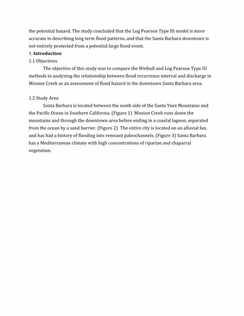
Santa Barbara is located between the south side of the Santa Ynez Mountains and

the Pacific Ocean in Southern California. (Figure 1) Mission Creek runs down the

mountains and through the downtown area before ending in a coastal lagoon, separated

from the ocean by a sand barrier. (Figure 2) The entire city is located on an alluvial fan,

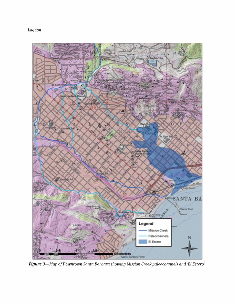
and has had a history of flooding into remnant paleochannels. (Figure 3) Santa Barbara

has a Mediterranean climate with high concentrations of riparian and chaparral

vegetation.

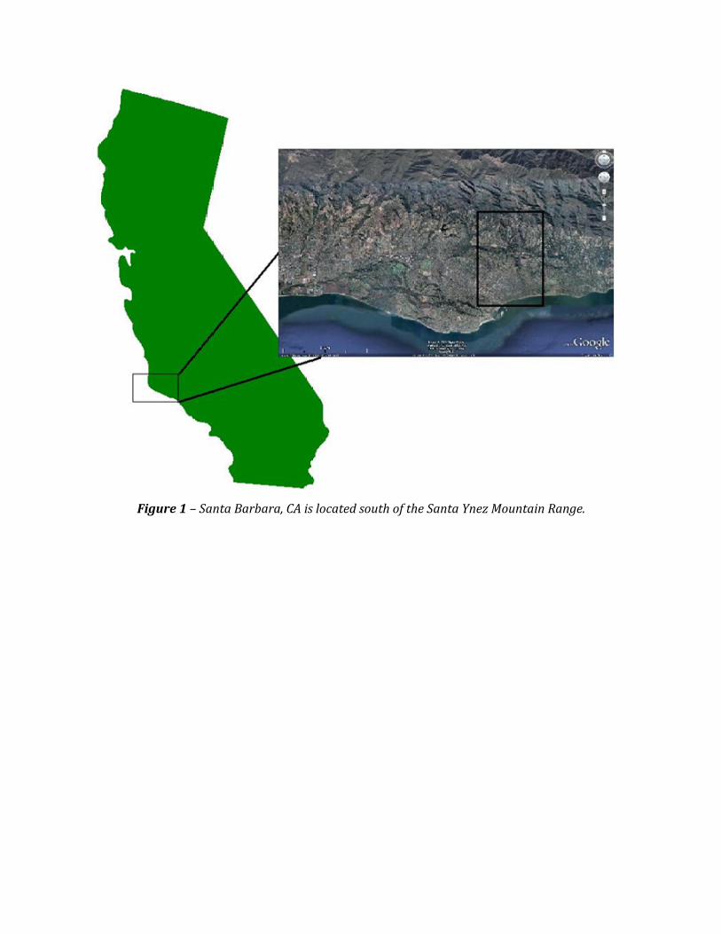
Figure 1 – Santa Barbara, CA is located south of the Santa Ynez Mountain Range.

Figure 2 – Mission Creek Watershed, Mission Creek, Rattlesnake Creek, Skofield Park Reach, Santa

Barbara Botanic Garden Reach, Rocky Nook Park reach, Oak Park Reach, Channelized Reach,

Lagoon

Figure 3—Map of Downtown Santa Barbara showing Mission Creek paleochannels and ‘El Estero’.

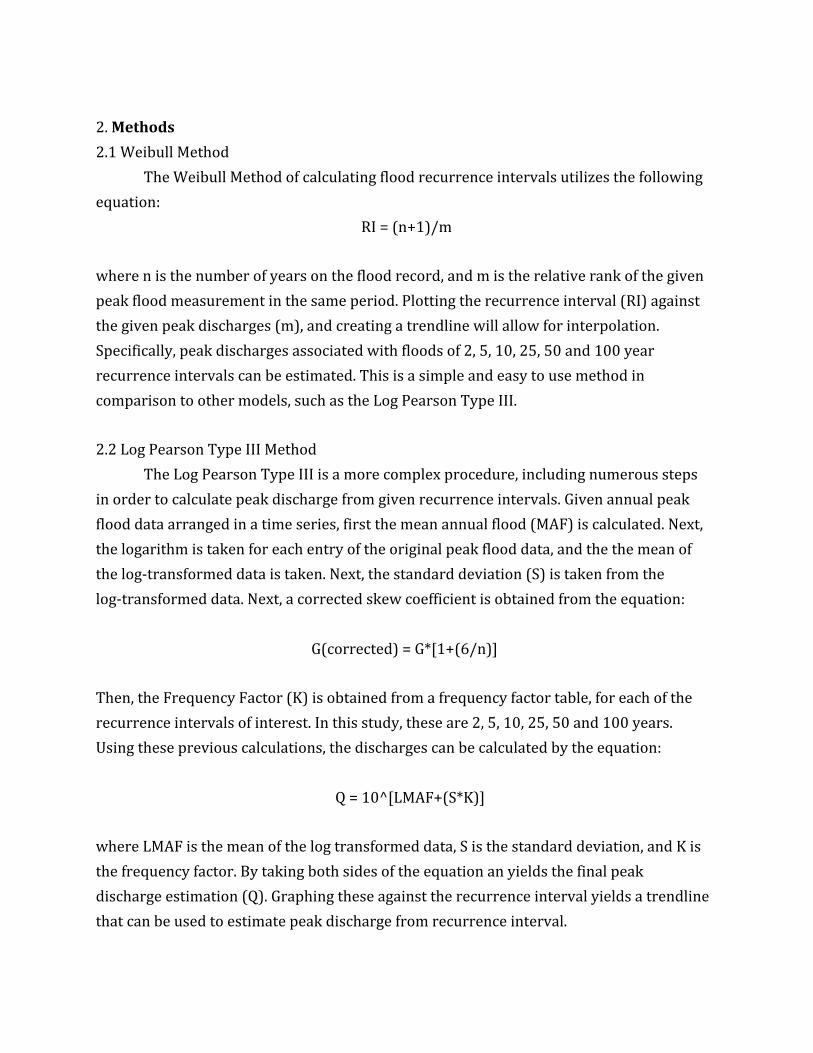
2. Methods

2.1 Weibull Method

The Weibull Method of calculating flood recurrence intervals utilizes the following

equation:

RI = (n+1)/m

where n is the number of years on the flood record, and m is the relative rank of the given

peak flood measurement in the same period. Plotting the recurrence interval (RI) against

the given peak discharges (m), and creating a trendline will allow for interpolation.

Specifically, peak discharges associated with floods of 2, 5, 10, 25, 50 and 100 year

recurrence intervals can be estimated. This is a simple and easy to use method in

comparison to other models, such as the Log Pearson Type III.

2.2 Log Pearson Type III Method

The Log Pearson Type III is a more complex procedure, including numerous steps

in order to calculate peak discharge from given recurrence intervals. Given annual peak

flood data arranged in a time series, first the mean annual flood (MAF) is calculated. Next,

the logarithm is taken for each entry of the original peak flood data, and the the mean of

the log-transformed data is taken. Next, the standard deviation (S) is taken from the

log-transformed data. Next, a corrected skew coefficient is obtained from the equation:

G(corrected) = G*[1+(6/n)]

Then, the Frequency Factor (K) is obtained from a frequency factor table, for each of the

recurrence intervals of interest. In this study, these are 2, 5, 10, 25, 50 and 100 years.

Using these previous calculations, the discharges can be calculated by the equation:

Q = 10^[LMAF+(S*K)]

where LMAF is the mean of the log transformed data, S is the standard deviation, and K is

the frequency factor. By taking both sides of the equation an yields the final peak

discharge estimation (Q). Graphing these against the recurrence interval yields a trendline

that can be used to estimate peak discharge from recurrence interval.

A second analysis included the estimation of flood recurrence interval from

historical flood discharge data in the Santa Barbara Mission Creek. The trendline equation

derived for discharge (Q) is rearranged to solve for recurrence interval (RI), and applied

to historical peak discharge values.

2.3 Laguna Drain

The Rational Method is used to estimate the discharge for minor (Q5) and major

(Q25) storm events in the Laguna Drain. The Rational Method is expressed in the

equation:

Q = CIA

where C is the peak discharge (cfs), I is the average rainfall intensity (inches per hour),

and A is the drainage area (acres). The Laguna Drain was designed to carry a peak

discharge of 950 cfs, so the calculations for storm event discharges will determine if the

drain can contain high flow events.

3. Data

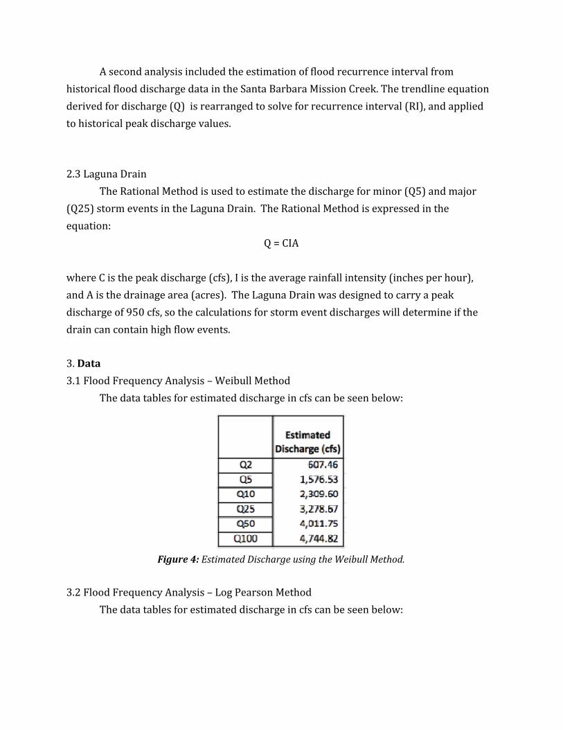
3.1 Flood Frequency Analysis – Weibull Method

The data tables for estimated discharge in cfs can be seen below:

Figure 4: Estimated Discharge using the Weibull Method.

3.2 Flood Frequency Analysis – Log Pearson Method

The data tables for estimated discharge in cfs can be seen below:

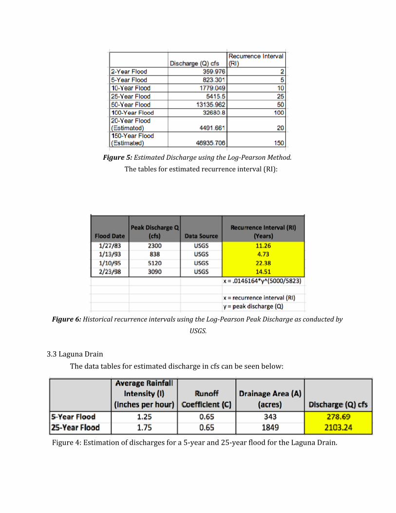
Figure 5: Estimated Discharge using the Log-Pearson Method.

The tables for estimated recurrence interval (RI):

Figure 6: Historical recurrence intervals using the Log-Pearson Peak Discharge as conducted by

USGS.

3.3 Laguna Drain

The data tables for estimated discharge in cfs can be seen below:

Figure 4: Estimation of discharges for a 5-year and 25-year flood for the Laguna Drain.

4. Discussion

4.1 Weibull and Log Pearson Type III Distribution Models

The Weibull and Log Pearson Type III distributions are two approaches used to

analyze flood frequency. The Log Pearson Type III is more complex than Weibull method,

and includes a logarithmic transformation. The Interagency Advisory Committee on

Water Data recommends the Log Pearson Type III as the standard model for flood

frequency studies in all U.S. Government agencies.

The Weibull distribution, also called “plotting position,” utilizes probabilities of

peak flood events to construct a flood frequency curve. Furthermore, the Weibull

distribution employs two parameters in describing the distribution (compared to Log

Pearson’s three). This limits the flexibility of use.

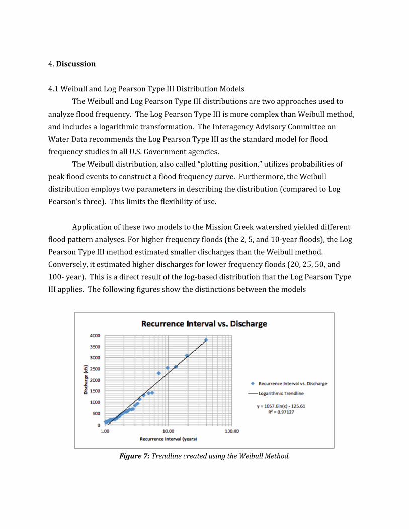
Application of these two models to the Mission Creek watershed yielded different

flood pattern analyses. For higher frequency floods (the 2, 5, and 10-year floods), the Log

Pearson Type III method estimated smaller discharges than the Weibull method.

Conversely, it estimated higher discharges for lower frequency floods (20, 25, 50, and

100- year). This is a direct result of the log-based distribution that the Log Pearson Type

III applies. The following figures show the distinctions between the models

Figure 7: Trendline created using the Weibull Method.

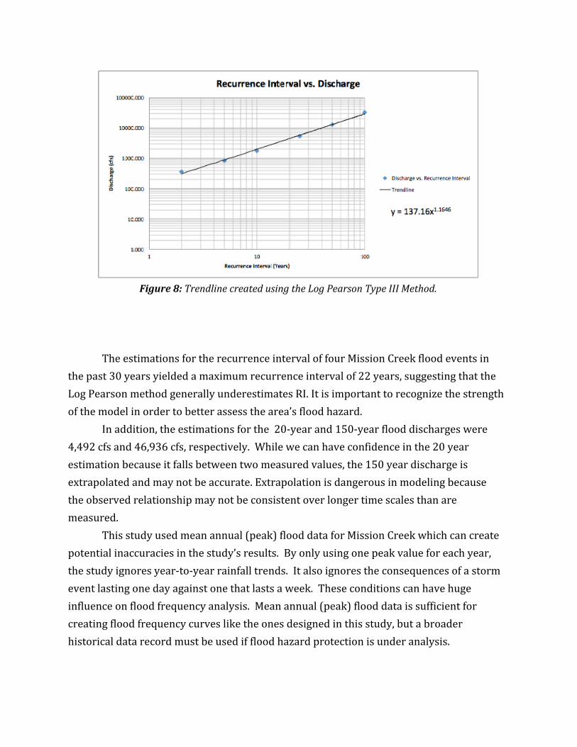
Figure 8: Trendline created using the Log Pearson Type III Method.

The estimations for the recurrence interval of four Mission Creek flood events in

the past 30 years yielded a maximum recurrence interval of 22 years, suggesting that the

Log Pearson method generally underestimates RI. It is important to recognize the strength

of the model in order to better assess the area’s flood hazard.

In addition, the estimations for the 20-year and 150-year flood discharges were

4,492 cfs and 46,936 cfs, respectively. While we can have confidence in the 20 year

estimation because it falls between two measured values, the 150 year discharge is

extrapolated and may not be accurate. Extrapolation is dangerous in modeling because

the observed relationship may not be consistent over longer time scales than are

measured.

This study used mean annual (peak) flood data for Mission Creek which can create

potential inaccuracies in the study’s results. By only using one peak value for each year,

the study ignores year-to-year rainfall trends. It also ignores the consequences of a storm

event lasting one day against one that lasts a week. These conditions can have huge

influence on flood frequency analysis. Mean annual (peak) flood data is sufficient for

creating flood frequency curves like the ones designed in this study, but a broader

historical data record must be used if flood hazard protection is under analysis.

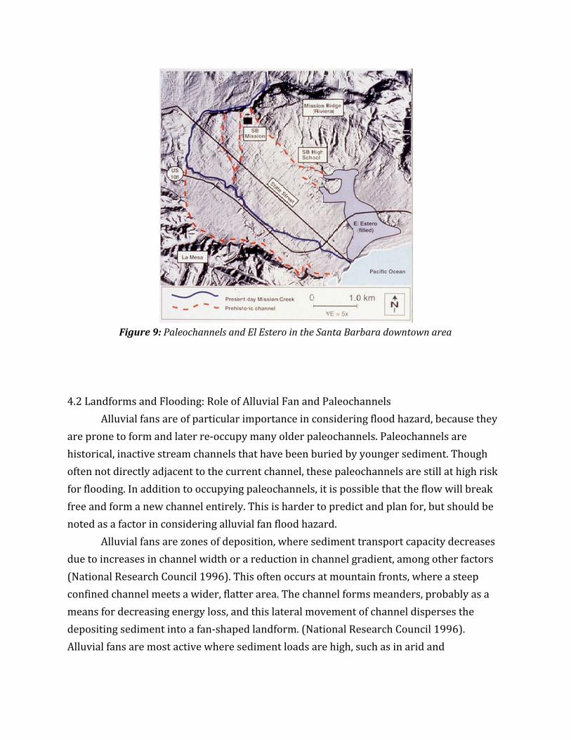
Figure 9: Paleochannels and El Estero in the Santa Barbara downtown area

4.2 Landforms and Flooding: Role of Alluvial Fan and Paleochannels

Alluvial fans are of particular importance in considering flood hazard, because they

are prone to form and later re-occupy many older paleochannels. Paleochannels are

historical, inactive stream channels that have been buried by younger sediment. Though

often not directly adjacent to the current channel, these paleochannels are still at high risk

for flooding. In addition to occupying paleochannels, it is possible that the flow will break

free and form a new channel entirely. This is harder to predict and plan for, but should be

noted as a factor in considering alluvial fan flood hazard.

Alluvial fans are zones of deposition, where sediment transport capacity decreases

due to increases in channel width or a reduction in channel gradient, among other factors

(National Research Council 1996). This often occurs at mountain fronts, where a steep

confined channel meets a wider, flatter area. The channel forms meanders, probably as a

means for decreasing energy loss, and this lateral movement of channel disperses the

depositing sediment into a fan-shaped landform. (National Research Council 1996).

Alluvial fans are most active where sediment loads are high, such as in arid and

structurally weak mountain regions (National Research Council 1996). These conditions

are consistent with the Santa Barbara Mission Creek study area.

In Mission Creek low flow conditions, flow is confined to a single channel. In high

flow conditions, such as those caused by large precipitation events, discharge may exceed

the main channel’s capacity and be diverted into remnant paleochannels. (Figure 9) Many

of the paleochannels in the downtown Santa Barbara area are due to the Mission Ridge

Fault, which diverts Mission Creek as it propagates westward. Flow paths are cut as the

present channel down-cuts the anticline. This creates wind gaps when the paleochannels

are empty, and water gaps where flow is experienced.

Presently, Mission Creek runs along the south west boundary of the downtown

Santa Barbara area and ends in a small coastal lagoon by Stearn’s Wharf. (Figure 9)

However historically, Mission Creek flowed into El Estero, a large coastal lagoon that once

resided on the northeastern side of downtown. The paleochannels that once emptied into

this lagoon run directly through the downtown area, and are therefore a cause for

concern. Similarly, the area previously occupied by El Estero is subject to flooding and is

cause for concern as well.

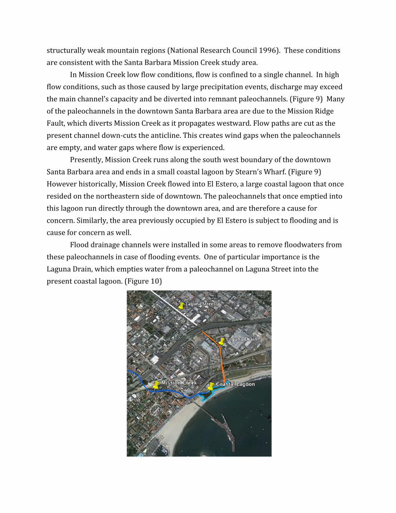
Flood drainage channels were installed in some areas to remove floodwaters from

these paleochannels in case of flooding events. One of particular importance is the

Laguna Drain, which empties water from a paleochannel on Laguna Street into the

present coastal lagoon. (Figure 10)

Figure 10: Location of Laguna Drain. Created using Google Earth.

4.3 Main reasons for flood hazard in Santa Barbara

Santa Barbara has a long history of flood events. Between 1862 and 2010, Santa

Barbara experienced 15 significant floods, eight of which received Presidential Disaster

Declarations (Abrams 2012). While flood hazard prevention measures have been taken,

the uncertainty associated with the size, location, and type of flood event increase the

potential hazard. The processes of sediment transport and deposition are especially

important, as they can potentially alter the flow path and create debris flow conditions.

During high discharge events, the abrupt deposition of sediment or debris during a

flood may substantially alter hydraulic conditions and initiate new, distinct flow paths of

uncertain direction (Larson, 2000). This uncertainty is dangerous because it is difficult to

predict and therefore difficult to prepare for. While high risk areas are focuses of flood

proofing and flood preparation efforts, the creation of new flow paths would affect

unprepared areas and therefore pose a larger hazard of human and property damage.

In addition, sediment deposition increases the risk of landslides and debris flows.

In Santa Barbara, the risk of debris flow is minimized by the high stability of sediment in

the Mission Creek tributaries. However, if a flood event were to occur after a fire event,

which creates large volumes of sediment, the potential for a debris flow would be

significantly increase. Due to the high recurrence of fires in the area, it is important to

consider this possibility.

Flow path uncertainty and debris flow potential are major factors in considering

the Santa Barbara flood hazard.

4.4 How the Santa Barbara flood hazard might be minimized

Planning

flood proofing

infrastructure

urban runoff prevention

Emergency response

spatial modeling

Cities built on alluvial fans such as Santa Barbara must develop flood hazard

protection projects to protect the city from flooding. Projects that have been completed in

recent years reveal an acknowledgment of the comprehensive reform that must occur to

mitigate the significant local hazard of flooding.

In mitigating the flood hazard,

Santa Barbara County’s Office of Emergency Management has summarized the

city’s aim for flood hazard protection in the “2011 Multi-Jurisdiction Hazard Mitigation

Plan.” Its three major goals include promoting disaster-resistant future development,

building and supporting capacity and commitment to existing infrastructure to become

less vulnerable to hazards, and enhance hazard mitigation coordination and

communication. The report also details significant flood control work in progress,

including improvements of storm drain and channelization infrastructure.

The Laguna Drain, a concrete, trapezoidal channel that collects urban runoff, was

designed to carry a peak flow of 950 cfs (Keller 2013). This would be sufficient to carry

the estimated 5 year discharge of 823 cfs. However, in considering the estimated 25 year

discharge of 2100 cfs, the Laguna drain would be insufficient to carry the flow. This

suggests that the downtown area is vulnerable to flooding if Mission Creek re-occupies

one of its paleochannels. Because the creek has been known to reoccupy its

paleochannels during large flood events, this could pose a significant danger. In order to

offset the inability of the channel to accommodate the 25-year flood discharge, flood

hazard mapping, monitoring the progress or storms, channel modifications

(channelization and engineering approaches) and regulatory approaches to reduce

vulnerability. (Nelson, 2012)

Flood hazard mapping can be used to assess susceptible areas to flooding. By

using historical data on rivers and discharges, as well as topographical data, flood-hazard

maps can be created that will spatially visualize regions of the area that would be

expected to be affected by the various discharges and recurrence intervals. (Nelson,

2012) Geographical information systems/science would be able to highlight the regions

of this report’s study area, such as in the image below:

Figure 11: Map visualizing the impact of various recurrence intervals and discharge stages.

By monitoring the progress of storms with geographical information

systems/science (GIS) to determine significant factors such the degree of ground

saturation, amount of vegetation, amount of rainfall or the degree of permeable soil, a

relationship from the integration of the various factors can result in short-term

prediction. (Nelson, 2012) Comprehensive forecasting can result in flash flood warning

being issued to the affected areas.

Channels are dynamic systems that modify themselves in response to changes in

physical watershed features regardless of human involvement. Channel modifications

include deepening, widening, straightening, and construction of new channels. (Figure 12)

Figure 12: Cross-section of channelization methods.

Other engineering approaches include dams, retention ponds, levees and

floodways. Dams are able to store a volume of water to encourage retention and can be

regulated to be released at a desired rate (Nelson, 2012). Retention ponds also serve a

purpose that is akin to those that dams accommodate for, by trapping water and releasing

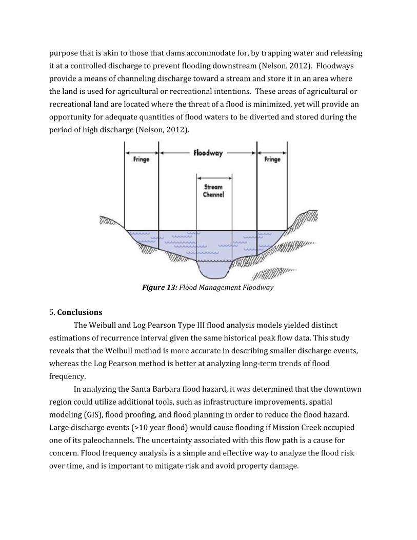
it at a controlled discharge to prevent flooding downstream (Nelson, 2012). Floodways

provide a means of channeling discharge toward a stream and store it in an area where

the land is used for agricultural or recreational intentions. These areas of agricultural or

recreational land are located where the threat of a flood is minimized, yet will provide an

opportunity for adequate quantities of flood waters to be diverted and stored during the

period of high discharge (Nelson, 2012).

Figure 13: Flood Management Floodway

5. Conclusions

The Weibull and Log Pearson Type III flood analysis models yielded distinct

estimations of recurrence interval given the same historical peak flow data. This study

reveals that the Weibull method is more accurate in describing smaller discharge events,

whereas the Log Pearson method is better at analyzing long-term trends of flood

frequency.

In analyzing the Santa Barbara flood hazard, it was determined that the downtown

region could utilize additional tools, such as infrastructure improvements, spatial

modeling (GIS), flood proofing, and flood planning in order to reduce the flood hazard.

Large discharge events (>10 year flood) would cause flooding if Mission Creek occupied

one of its paleochannels. The uncertainty associated with this flow path is a cause for

concern. Flood frequency analysis is a simple and effective way to analyze the flood risk

over time, and is important to mitigate risk and avoid property damage.

Works Cited

Abrams, Richard. 2011 Santa Barbara County Multi-jurisdictional Hazard Mitigation Plan.

County of Santa Barbara. 2011. ftp://pwftp.countyofsb.org/Water/FTP/State

request/Flood management/Multi_hazard Report/Cover Page 2011.pdf

Analysis techniques: Flood frequency analysis. Civil, Construction and Environmental

Engineering Department. Oregon State University. Corvallis, OR. 2005.

http://streamflow.engr.oregonstate.edu/analysis/floodfreq/

Bengtson, Harlan. Hydrology (Part2)- Frequency Analysis of Flood Data. Continuing

Education and Development, Inc. 2012.

http://www.cedengineering.com/upload/Hydrology%202%20-%20Flood%20Data.pdf

Keller, E. Lab 3: Flood Hazard Analysis. Environmental Studies 144: Rivers. University of

California, Santa Barbara. 2013.

Larson, Matthew et. al. The Natural Hazards on Alluvial Fans: the Venezuela Debris Flow

and Flash Flood Disaster. USGS. 2000. http://pubs.usgs.gov/fs/fs-0103-01/fs-0103-01.pdf

National Research Council. Alluvial Fan Flooding. The National Academies Press.

Washington DC. 1996.

Nelson, S. (2012). Flooding hazards, prediction & human intervention. Unpublished

manuscript, Earth and Environmental Sciences, Tulane University, Retrieved from

http://www.tulane.edu/~sanelson/Natural_Disasters/floodhaz.htm

Equations

● RI = (n+1)/m

● G(corrected) = G*[1+(6/n)]

● Q = 10^[LMAF+ (S*K)]