Embed Size (px)
Citation preview

www.rcmt.cvut.cz
CZECH TECHNICAL UNIVERSITY IN PRAGUE | FACULTY OF MECHANICAL ENGINEERING
Department of Production Machines and Equipment | PME
Research Center of Manufacturing Technology | RCMT
Viktor Kulíšek
Finite element analysis of
composite structures
14.12.2016

2
Overview – FEA of composite structures
● Introduction
– Typical composite applications
● Composite materials
– Fibre and matrix properties
– Fabrics and preforms
● Unidirectional composite
– Material properties
● Layered structures
– ABD matrix and its implications
● FEA of composite structures
– Elements for FEA of composites
– Stress and strength
● Examples
3
Introduction – FEA of composite structures
● Finite element analysis of composite structures
– The principle of FEA same as for the isotropic materials from the previous
courses
K. 𝑢 = 𝑓
– K global stiffness matrix
– u global vector of nodal displacements
– f global vector of external equivalent nodal forces
solution: 𝑢 = 𝐾−1. 𝑓
– For composite structures more challenging in pre-processing of models and
post-processing of results
• Due to orthotropic behaviour of material and other important parameters
– In this lecture, the basic approaches for modelling of long fibre reinforced
plastics are discussed
4
Introduction – FEA of composite structures
● Important to know
– What are the demanded results of the simulation?
(stress, displacement, natural frequencies, temperature distribution, crash
behaviour, …)
– What is the demanded precision of results?
– What manufacturing technology and preforms are used for the structure?
• fabrics, prepregs, fibre tows
• unidirectional versus multidirectional preform
• abilities of manufacturing technology
● Important decisions
– Elements type selection and geometry simplifications
– Modelling of composite structure
• full composite lay-up
• ABD matrix
• properties homogenization
5
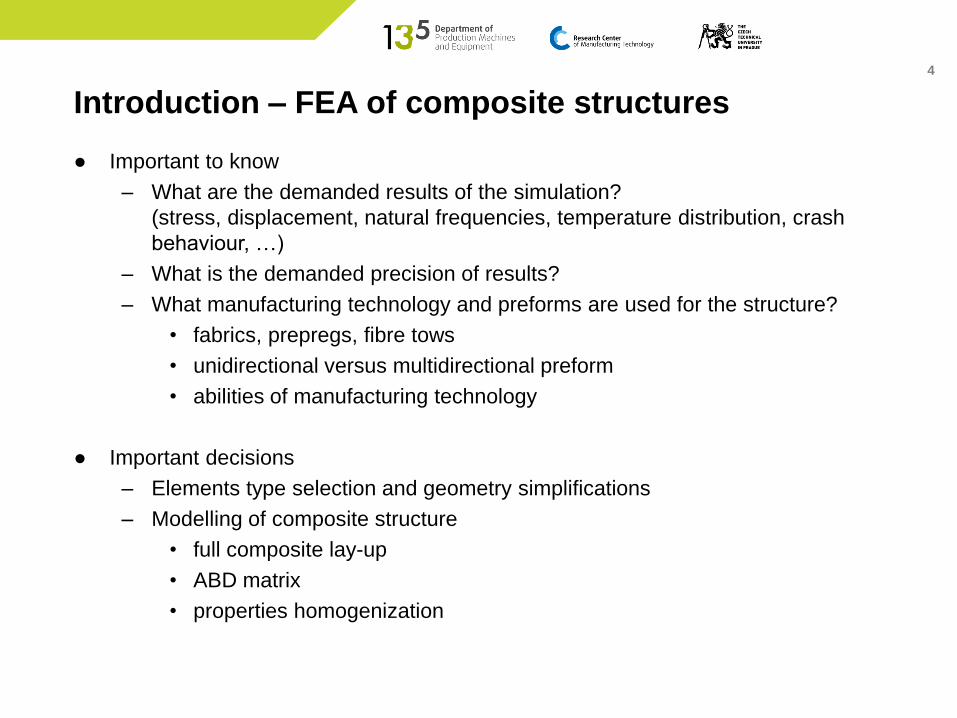
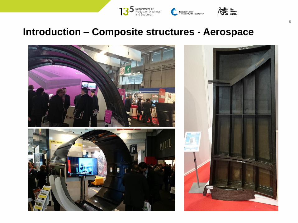
Introduction – Composite structures - Aerospace
● Airbus 350XBW, Premium AEROTEC
6
Introduction – Composite structures - Aerospace
7
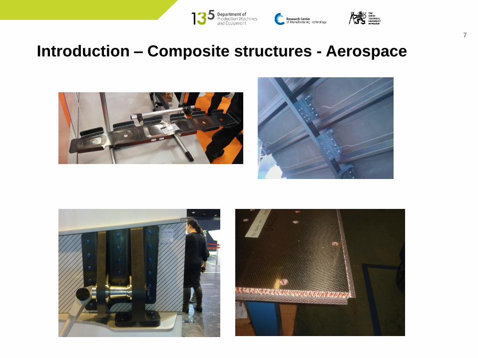
Introduction – Composite structures - Aerospace
8
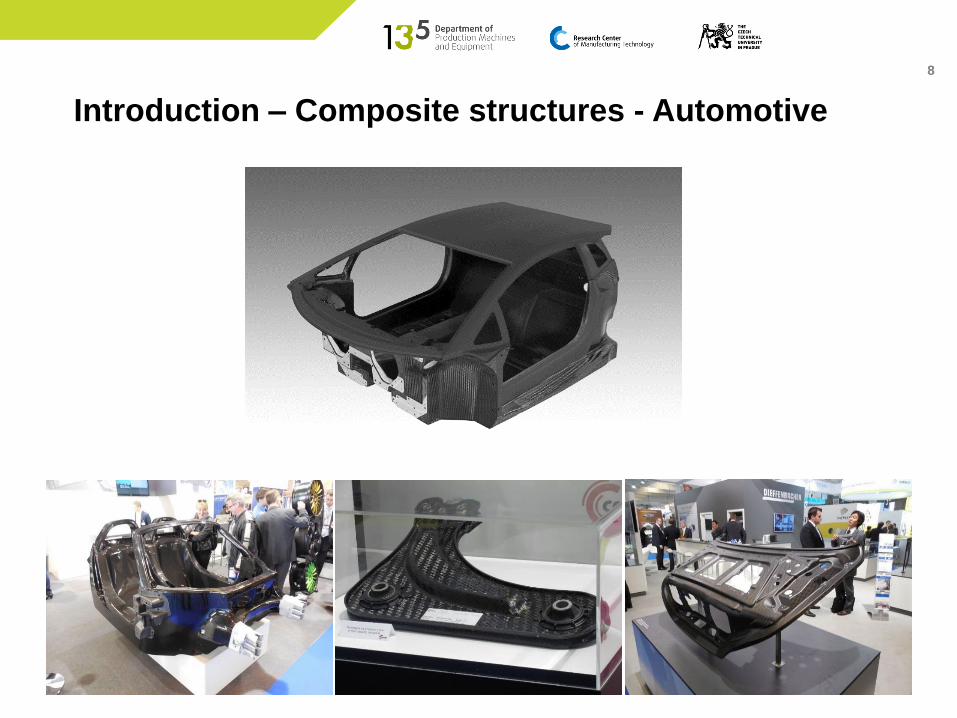
Introduction – Composite structures - Automotive
9
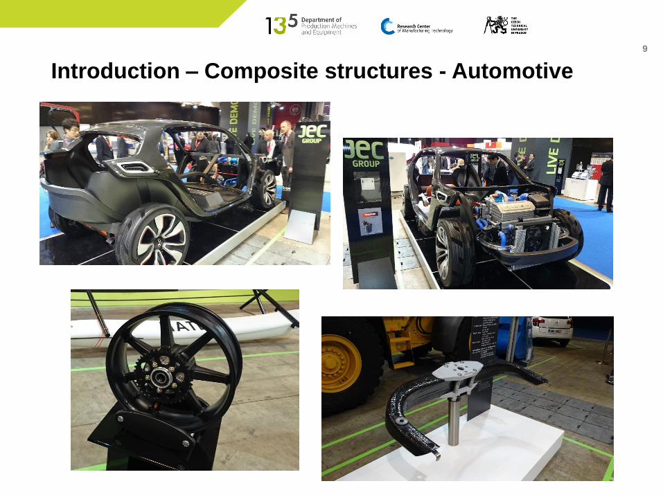
Introduction – Composite structures - Automotive
10
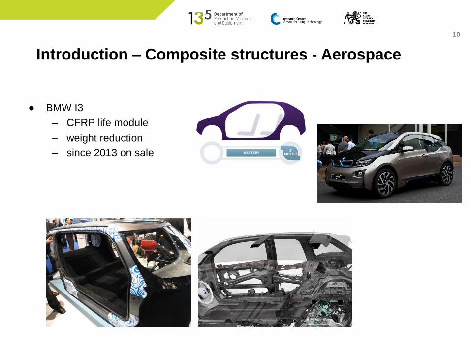
● BMW I3
– CFRP life module
– weight reduction
– since 2013 on sale
Introduction – Composite structures - Aerospace

11
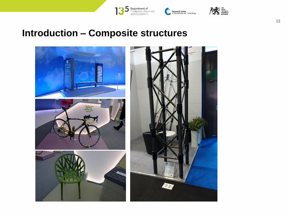
Introduction – Composite structures - Industry
12
Introduction – Composite structures

13
Introduction
● Short conclusions in terms of composite structures
– Usually thin components (thickness is significantly smaller than other 2
dimensions)
• Suitable for shell elements, beam elements
• Options for solid modelling limited
– Usually composite lay-up with layers with multiangle orientations, structures
with only 1 orientation of fibres are rare
– Various semi-finished products used in the structures
• Fabrics, prepregs, rovings
• Different manufacturing technologies, different fibre volume fraction in
the composite layer
– Various materials used in applications
• Fibres
• Matrices
– All of the aforementioned influence the behaviour of the component and
thereby the demands for its modelling

14
Composite materials
● Demonstration – layer of composite material
● Properties of layer is determined by
– type of fibre
• carbon, glass, boron, aramid
– type of matrix
• thermosets - epoxy,…
• thermoplastics – PA12, PEEK, PPS,...
– type of semi-finished product
• unidirectional
• multidirectional
– fibre volume fraction in the layer
• manufacturing technology
15
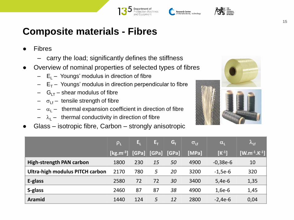
Composite materials - Fibres
● Fibres
– carry the load; significantly defines the stiffness
● Overview of nominal properties of selected types of fibres
– EL – Youngs’ modulus in direction of fibre
– ET – Youngs’ modulus in direction perpendicular to fibre
– GLT – shear modulus of fibre
– sLf – tensile strength of fibre
– aL – thermal expansion coefficient in direction of fibre
– lL – thermal conductivity in direction of fibre
● Glass – isotropic fibre, Carbon – strongly anisotropic
rL
[kg.m-3]
EL
[GPa]
ET
[GPa]
Gf
[GPa]
sLf
[MPa]
aL
[K-1]
lLf
[W.m-1.K-1]
High-strength PAN carbon 1800 230 15 50 4900 -0,38e-6 10
Ultra-high modulus PITCH carbon 2170 780 5 20 3200 -1,5e-6 320
E-glass 2580 72 72 30 3400 5,4e-6 1,35
S-glass 2460 87 87 38 4900 1,6e-6 1,45
Aramid 1440 124 5 12 2800 -2,4e-6 0,04
16
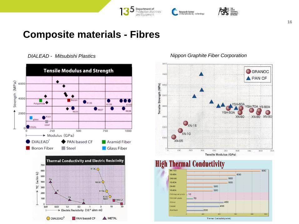
DIALEAD - Mitsubishi Plastics Nippon Graphite Fiber Corporation
Composite materials - Fibres

17
Composite materials - Matrices
● Matrix
– affects strength, fracture toughness
– affects other properties (flammability, conductivity, fatigue,
biocompactibility, …)
– determines/restricts the manufacturing technologies
● Thermosets
– non-repeatable manufacturing
process
• after curing no reshaping (non-
destructively)
– longer time of curing (hours…
minutes)
– brittle materials
– …
● Thermoplastics
– repeatable manufacturing
process
• after heating – matrix
softening – reshaping
– short time of processing
(minutes)
– good fracture toughness
– …

18
Composite materials - Matrices
Source: RED, Chris. The Outlook for Thermoplastics in Aerospace Composites, 2014-2023. In High-
Performance Composites. Vol. 22, No. 5, 2014.

19
Composite materials - Matrices
MatrixDensity[kg.m-3]
E[MPa]
a
[K-1]l
[W/m/K]
Glass transition temp. [°C]
Melting temp.
[°C]
Epoxy 1150 2600÷5000 60e-6 0,2÷0,5 50÷200 x
Non-saturated polyesters
1170÷1260 14000÷20000 20÷40e-6 0,3÷0,7 60÷170 x
Phenolicresins
1400÷1800 5600÷12000 15÷50e-6 0,4÷0,7 70÷120 x
PP 900 1300-1800 130÷180e-6 0,17÷0,25 -20÷20 160÷165
PA6 1150 2800 80÷90e-6 0,22÷0,3 45÷80 225÷235
PA12 1004 1400 120÷140e-6 0,22÷0,24 40÷50 170÷180
PPS 1350 3700 50÷70e-6 x 85÷100 275÷290
PEEK 1300 3700 50÷70e-6 0,25 145÷155 335÷345
PEI 1270 3000 50e-6 0,22 215÷230 x
20
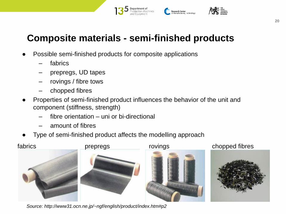
rovingsfabrics prepregs chopped fibres
● Possible semi-finished products for composite applications
– fabrics
– prepregs, UD tapes
– rovings / fibre tows
– chopped fibres
● Properties of semi-finished product influences the behavior of the unit and
component (stiffness, strength)
– fibre orientation – uni or bi-directional
– amount of fibres
● Type of semi-finished product affects the modelling approach
Source: http://www31.ocn.ne.jp/~ngf/english/product/index.htm#p2
Composite materials - semi-finished products

21
● Fabrics
– plain
• worse drapability
• good strength, resistance against
shift of fibres
– twill
• average drapability
– satin
• good drapability
• small resistance against shift of fibres
Composite materials - semi-finished products
22
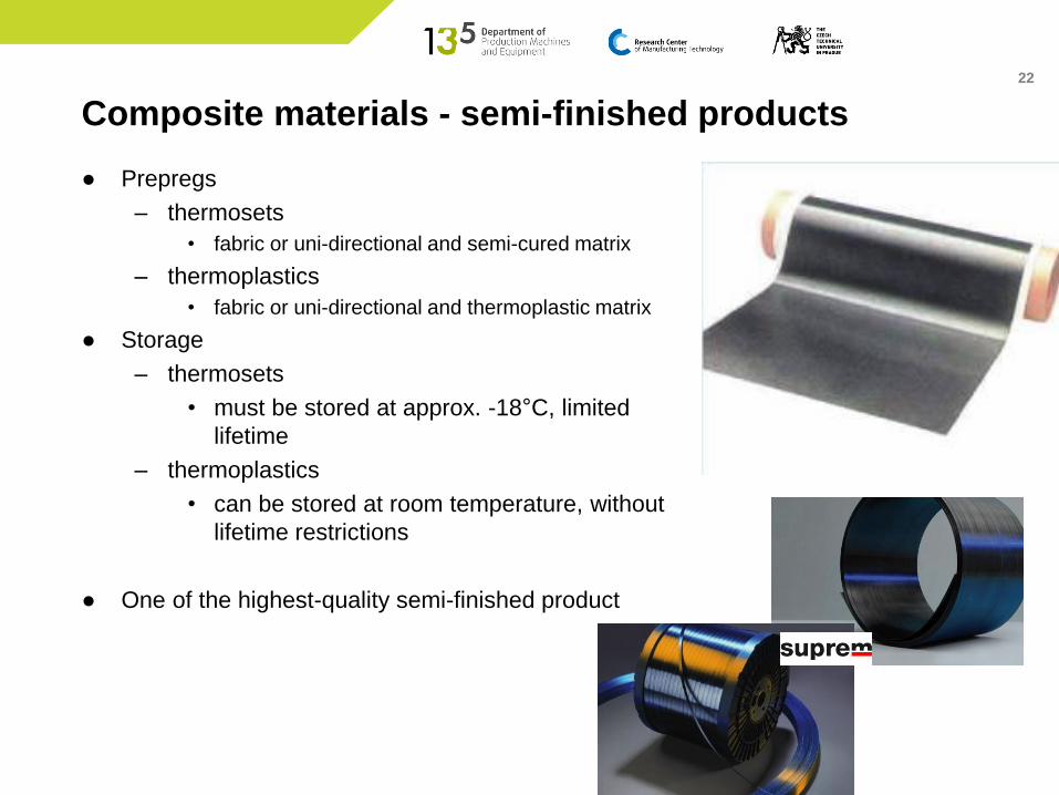
Composite materials - semi-finished products
● Prepregs
– thermosets
• fabric or uni-directional and semi-cured matrix
– thermoplastics
• fabric or uni-directional and thermoplastic matrix
● Storage
– thermosets
• must be stored at approx. -18°C, limited
lifetime
– thermoplastics
• can be stored at room temperature, without
lifetime restrictions
● One of the highest-quality semi-finished product
23
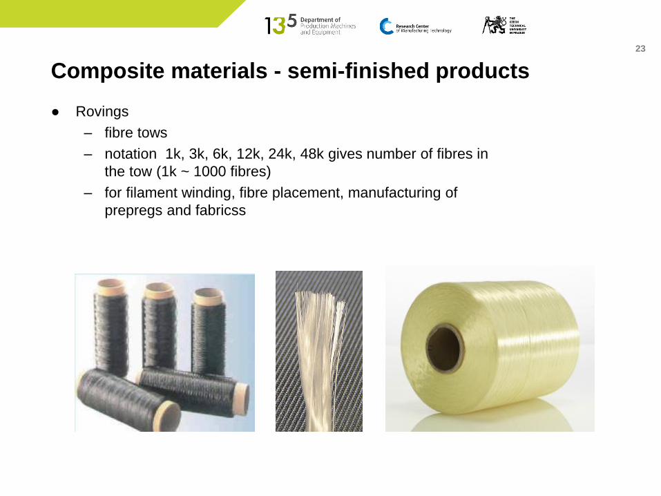
Composite materials - semi-finished products
● Rovings
– fibre tows
– notation 1k, 3k, 6k, 12k, 24k, 48k gives number of fibres in
the tow (1k ~ 1000 fibres)
– for filament winding, fibre placement, manufacturing of
prepregs and fabricss
24
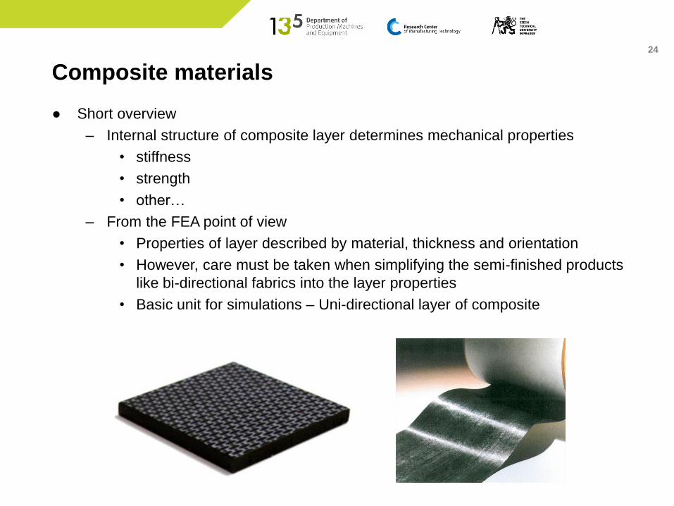
Composite materials
● Short overview
– Internal structure of composite layer determines mechanical properties
• stiffness
• strength
• other…
– From the FEA point of view
• Properties of layer described by material, thickness and orientation
• However, care must be taken when simplifying the semi-finished products
like bi-directional fabrics into the layer properties
• Basic unit for simulations – Uni-directional layer of composite
25
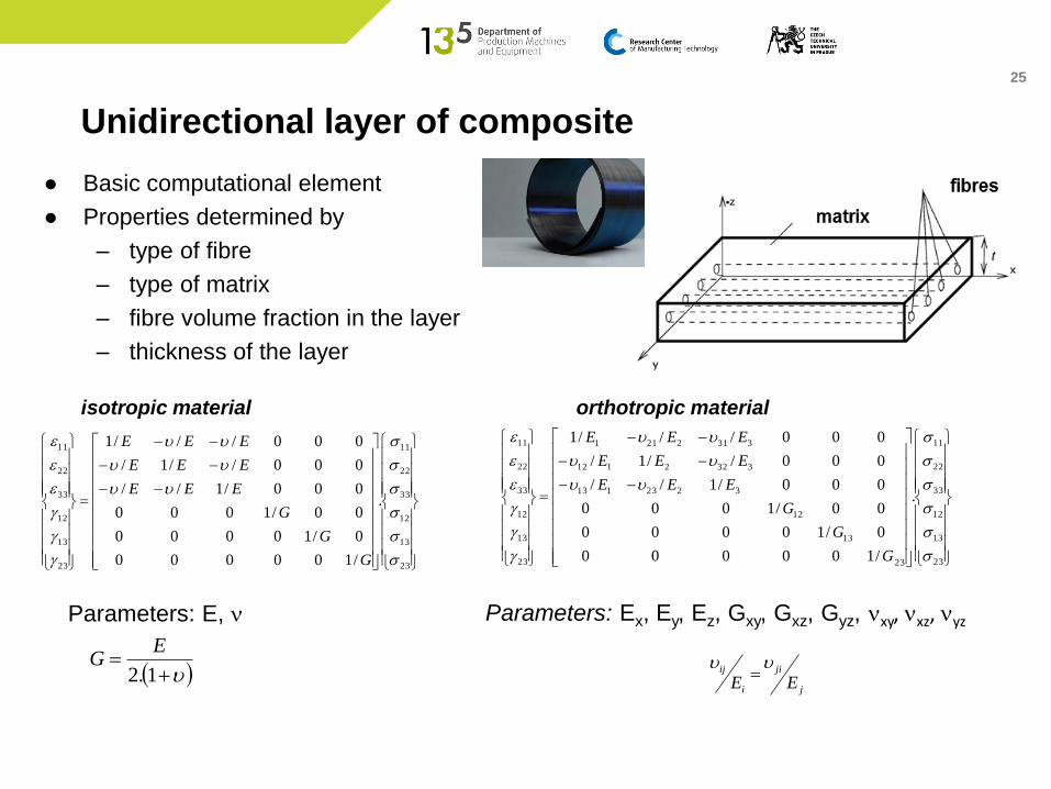
● Basic computational element
● Properties determined by
– type of fibre
– type of matrix
– fibre volume fraction in the layer
– thickness of the layer
23
13
12
33
22
11
23
13
12
33
22
11
.
/100000
0/10000
00/1000
000/1//
000//1/
000///1
s
s
s
s
s
s
G
G
G
EEE
EEE
EEE
isotropic material
23
13
12
33
22
11
23
13
12
3223113
3322112
3312211
23
13
12
33
22
11
.
/100000
0/10000
00/1000
000/1//
000//1/
000///1
s
s
s
s
s
s
G
G
G
EEE
EEE
EEE
orthotropic material
1.2
EG
Parameters: E, n Parameters: Ex, Ey, Ez, Gxy, Gxz, Gyz, nxy, nxz, nyz
j
ji
i
ij
EE
Unidirectional layer of composite

26
● Material properties must fulfil stability criterion
23
13
12
33
22
11
23
13
12
33
22
11
.
/100000
0/10000
00/1000
000/1//
000//1/
000///1
s
s
s
s
s
s
G
G
G
EEE
EEE
EEE
isotropic material
23
13
12
33
22
11
23
13
12
3223113
3322112
3312211
23
13
12
33
22
11
.
/100000
0/10000
00/1000
000/1//
000//1/
000///1
s
s
s
s
s
s
G
G
G
EEE
EEE
EEE
orthotropic material
1.2
EG
Parameters: E, n Parameters: Ex, Ey, Ez, Gxy, Gxz, Gyz, nxy, nxz, nyz
j
ji
i
ij
EE
j
iij E
E
E>0, G>0Ei>0, Gij>0 i,j=x,y,z
021 xzzyyzxZzxzyyzyxxy
5,01
Unidirectional layer of composite
Conditions of stability

27
23
13
12
33
22
11
23
13
12
3223113
3322112
3312211
23
13
12
33
22
11
.
/100000
0/10000
00/1000
000/1//
000//1/
000///1
s
s
s
s
s
s
G
G
G
EEE
EEE
EEE
orthotropic material model
Parameters:
Ex, Ey, Ez, Gxy, Gxz, Gyz, nxy, nxz, nyz
12
22
11
12
2112
2211
12
2
1
/100
0/1/
0//1
s
s
s
G
EE
EE
lamina material model (plane stress)
Parameters:
Ex, Ey Gxy, nxy, (Gxz, Gyz)
Unidirectional layer of composite
● Thin composite structures
– neglecting through thickness stresses – plane stress model
– enable to simplify the model for composite laminates
● Although 4 parameters are necessary (Ex, Ey, Gxy, nxy), the other two shear
modules should be included as well
– due to low values of shear modulus of fibre composites
– to prevent unreasonable deformations of finite element model

28
● Modelling of UD layer
– thickness
– material properties (Ex, Ey, Gxy, nxy,Gxz, Gyz)
– material orientation
• Abaqus – orientation must be specified for not isotropic material;
otherwise input will not pass solver check
• Ansys APDL – if not specified, orientation is taken from the global
coordinate system**
● Elements
– Shell elements
– Solid elements (full orthotropic material model needed)
• be careful for the transverse shearing stresses
– Beams
● In reality, most composite structures compose of layers (UD or bi-directional) with
various orientation
** for shell elements the situation is more complicated
Unidirectional layer of composite
29
Unidirectional layer of composite
● Mechanical properties of layer
– Necessity to input Ex, Ey, Gxy, nxy, Gxz, Gyz
– How to get these constants?
• From the manufacturer of semi-finished product (prepregs)
• From experimental measurements
• By computation from fibre and matrix properties and assumed fibre
volume fraction (rule of mixture, micromechanics of composites)
– Issues
• Parameters of fibres can be unknown (mostly parameters in transverse
direction)
• Micromechanical model or rule of mixture might not correspond to the
selected fibre
– Different models for isotropic fibres (glass) and orthotropic fibres
– Variation between the models and experimental behaviour
• Theoretical fibre volume fraction does not match with the fibre volume
fraction of real composite component
• Different tensile and compressive modulus Ex of carbon fibre composites
(approx. 10%)

30
Unidirectional layer of composite
● Mechanical properties of layer
– Necessity to input Ex, Ey, Gxy, nxy, Gxz, Gyz
– Example of rule of mixture
• presented equations the most simple, not necessary the most accurate
1L f f f m
E V E V E 1
1 1
m m
T
fm
f
f
E EE
VEV
E
11 1
m m
LT
fm
f
f
G GG
VGV
G
LT f f m mV Vn n n
● Longitudinal modulus of layer
● In-plane Poisson number
● Transverse modulus of layer
● In-plane Shear modulus

31
● Transverse modulus of layer*
● In-plane Shear modulus*
Unidirectional layer of composite
● Mechanical properties of layer
– Necessity to input Ex, Ey, Gxy, nxy, Gxz, Gyz
– Should the factors like the fibre properties be included in the selection of the
mechanical model?
11 1
m m
T
fm
f
f
E EE
VEV
E
11 1
m m
LT
fm
f
f
G GG
VGV
G
● Transverse modulus of layer
● In-plane Shear modulus
𝐸T =𝐸𝑚
1 − 1 −𝐸𝑚𝐸𝑓𝑇
. 𝑉𝑓
𝐺LT =𝐺𝑚
1 − 𝑉𝑓. 1 −𝐺𝑚𝐺𝑓𝐿𝑇
* Equations – Chamis model, CHAMIS, Christos C. Simplified Composite Micromechanics Equations for Strength, Fracture
Toughness and Environmental Effects. Houston, January 1984. Report No. NASA TM-83696. National Aeronautics and Space
Administration.

32
Unidirectional layer of composite
● Mechanical properties of layer
– Ex, Ey, Gxy, nxy, Gxz, Gyz
– How to calculate other parameters
EZ, nxz, nyz, Gxz, Gyz ?
– Gyz, nyz – quite problematic
Gxy = Gxz = GLT
Ex = EL
Ey = Ez = ET
23
23/11 fm
m
GGV
GG
Chamis (B):Tsai (A):
m
f
f
f
ff
G
V
G
V
VVG
1
1
23
23
m
fmm GG
14
/43
Hashin
Gf23>Gm
m
mm
EK
213
mG
mK
mG
mK
fV
mG
fG
mG
fV
mGG
86
731
23
123
32
3
23
223
1212 nn
EEG

33
Unidirectional layer of composite
● Mechanical properties of layer
– Ex, Ey, Gxy, nxy, Gxz, Gyz
– How to calculate other parameters
EZ, nxz, nyz, Gxz, Gyz ?
– Gyz, nyz – quite problematic
Gxy = Gxz = GLT
Ex = EL
Ey = Ez = ET
23
23/11 fm
m
GGV
GG
Chamis (B):Tsai (A):
m
f
f
f
ff
G
V
G
V
VVG
1
1
23
23
m
fmm GG
14
/43
Hashin
Gf23>Gm
m
mm
EK
213
mG
mK
mG
mK
fV
mG
fG
mG
fV
mGG
86
731
23
123
32
3
23
223
1212 nn
EEG
34
Unidirectional layer of composite
● Effect of transverse shearing
– Bending of rectangular beam
bending transverse
shearing
Materialrf
[kg.m-3]
E1
[GPa]
G13
[GPa]
steel 7850 210 80
uhm/E 1750 380 3 (2÷4)
Beam of rectangular cross-section
– (EJ) – modulus E1
– (GA) – modulus G13
● For orthotropic beam profile low stiffness
in transverse shearing
– can be neglected when
length/thickness ratio is 30 (20) and
more
– increase of thickness not efficient,
need to change material orientation
𝑢 =𝐹. 𝐿3
3 𝐸𝐽+𝛽. 𝐹. 𝐿
𝐺𝐴
combination of
layers 0 and
[45,-45]s

35
Layered structures & Laminates
● Let’s get to reality
36
Layered structures & Laminates
● Real composite components – composed of layers with different orientations
– Hand made laminates
– Laminates from prepregs
– RTM products (resin transfer moulding)
– Filament or tape winding products, braiding
● In comparison with isotropic FE models
– Restriction of element types
– More time consuming preprocessing of the model
– More data consuming model
– Need to have clear idea what to do at the beginning of pre-processing
– Simplifications necessary, but might lead to fatal errors in modelling or post-
processing

37
Layered structures – Laminate theory
● Classical laminate theory
– relations between the load and
deformations of the laminate
– plane stress state in the laminate
– neglecting transverse shear stresses
– thickness of layer is significantly
smaller than other dimensions
– rigid interference between the layers
xy
y
x
xy
yy
xx
xy
y
x
xy
y
x
k
k
k
DDD
DDD
DDD
BBB
BBB
BBB
BBB
BBB
BBB
AAA
AAA
AAA
M
M
M
N
N
N
666261
262221
161211
666261
262221
161211
666261
262221
161211
666261
262221
161211
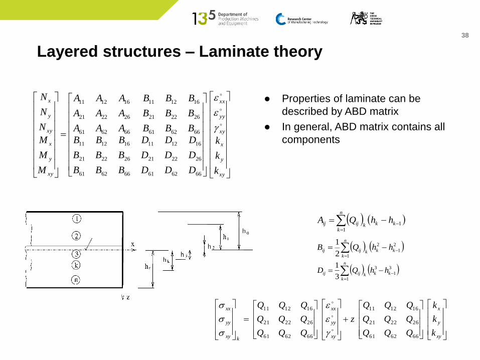
38
Layered structures – Laminate theory
● Properties of laminate can be
described by ABD matrix
● In general, ABD matrix contains all
components
xy
y
x
xy
yy
xx
xy
y
x
xy
y
x
k
k
k
DDD
DDD
DDD
BBB
BBB
BBB
BBB
BBB
BBB
AAA
AAA
AAA
M
M
M
N
N
N
666261
262221
161211
666261
262221
161211
666261
262221
161211
666261
262221
161211
3
1
3
13
1
kk
n
kkijij hhQD
xy
y
x
xy
yy
xx
kxy
yy
xx
k
k
k
QQQ
QQQ
QQQ
z
QQQ
QQQ
QQQ
666261
262221
161211
666261
262221
161211
s
s
s
2
1
2
12
1
kk
n
kkijij hhQB
1
1
kk
n
kkijij hhQA
39
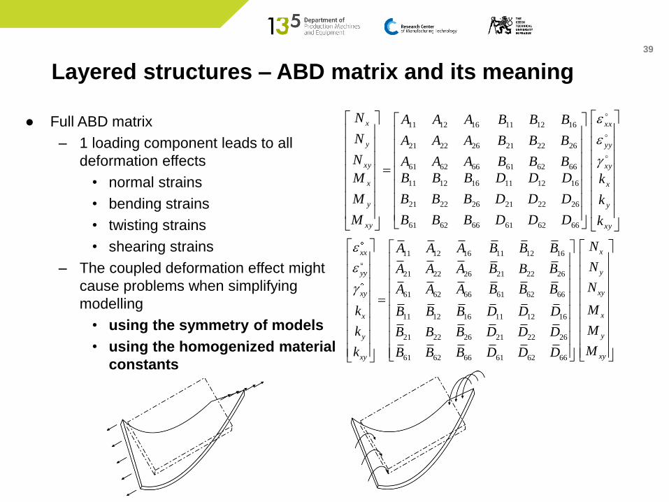
Layered structures – ABD matrix and its meaning
● Full ABD matrix
– 1 loading component leads to all
deformation effects
• normal strains
• bending strains
• twisting strains
• shearing strains
– The coupled deformation effect might
cause problems when simplifying
modelling
• using the symmetry of models
• using the homogenized material
constants
xy
y
x
xy
yy
xx
xy
y
x
xy
y
x
k
k
k
DDD
DDD
DDD
BBB
BBB
BBB
BBB
BBB
BBB
AAA
AAA
AAA
M
M
M
N
N
N
666261
262221
161211
666261
262221
161211
666261
262221
161211
666261
262221
161211
11 12 16 11 12 16
21 22 26 21 22 26
61 62 66 61 62 66
11 12 16 11 12 16
21 22 26 21 22 26
61 62 66 61 62 66
xxx
yyy
xyxy
xx
yy
xyxy
NA A A B B B
NA A A B B B
NA A A B B B
Mk B B B D D D
Mk B B B D D D
Mk B B B D D D

40
● Effect of composite lay-up on ABD matrix
662616
262212
161211
DDD
DDD
DDD
11
11
0 0
0 0
0 0 0
B
B
66
2212
1211
00
0
0
A
AA
AA
662616
262212
161211
BBB
BBB
BBB
000
000
000
B
11 12
12 22
66
0
0 0
D D
D D O
D
662616
262212
161211
DDD
DDD
DDD
662616
262212
161211
AAA
AAA
AAA
D A
Balanced
Symmetric balanced
Symmetric cross-ply
Antisymmetric cross-ply
Symmetric
.: 45 90 0 60 30S
Např
.: 30 60 0 60 30Např
66
2212
1211
00
0
0
A
AA
AA
000
000
000
662616
262212
161211
DDD
DDD
DDD
.: 30 30 60 60Např s
2.: 0 90 0 90 0Např
.: 0 90 0 90 0 90Např
66
2212
1211
00
0
0
A
AA
AA
66
2212
1211
00
0
0
A
AA
AA
000
000
000 11 12
12 22
66
0
0 0
D D
D D O
D
Layered structures – ABD matrix and its meaning
41
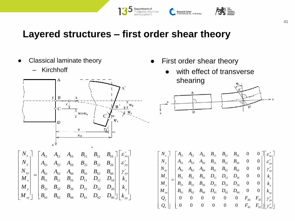
● Classical laminate theory
– Kirchhoff
xy
y
x
xy
yy
xx
xy
y
x
xy
y
x
k
k
k
DDD
DDD
DDD
BBB
BBB
BBB
BBB
BBB
BBB
AAA
AAA
AAA
M
M
M
N
N
N
666261
262221
161211
666261
262221
161211
666261
262221
161211
666261
262221
161211
● First order shear theory
● with effect of transverse
shearing
11 12 16 11 12 16
21 22 26 21 22 26
61 62 66 61 62 66
11 12 16 11 12 16
21 22 26 21 22 26
61 62 66 61 62 66
44 45
45 55
0 0
0 0
0 0
0 0
0 0
0 0
0 0 0 0 0 0
0 0 0 0 0 0
x
y
xy
x
y
xy
y
x
N A A A B B B
N A A A B B B
N A A A B B B
M B B B D D D
M B B B D D D
M B B B D D D
Q F F
Q F F
xx
yy
xy
x
y
xy
yz
xz
k
k
k
Layered structures – first order shear theory
42
11 12 16 11 12 16
21 22 26 21 22 26
61 62 66 61 62 66
11 12 16 11 12 16
21 22 26 21 22 26
61 62 66 61 62 66
44 45
45 55
0 0
0 0
0 0
0 0
0 0
0 0
0 0 0 0 0 0
0 0 0 0 0 0
x
y
xy
x
y
xy
y
x
N A A A B B B
N A A A B B B
N A A A B B B
M B B B D D D
M B B B D D D
M B B B D D D
Q F F
Q F F
xx
yy
xy
x
y
xy
yz
xz
k
k
k
● Transverse shearing
– can be neglected for very thin plates
– for composites, the length to
thickness ratio, from which it is
possible to neglect transverse
shearing, is significantly higher than
for isotropic materials
– FEA – shells generally with FOST
11 12 16
21 22 26
61 62 66
0
44 45
0
54 55
0 0
0 0
0 0
0 0 0
0 0 0
xx xx
yy yy
xy xy
yz yz
xz xzk
Q Q Q
Q Q Q
Q Q Q
C C
C C
s
s
s
s
s
Layered structures – first order shear theory
5,4, ,1
1
jihhCF kk
n
kkijij
43
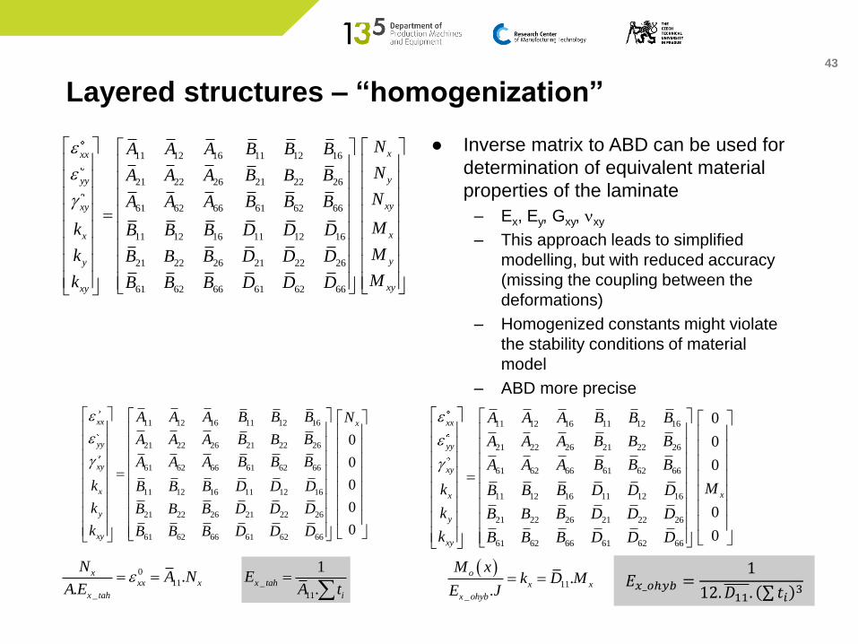
Layered structures – “homogenization”
● Inverse matrix to ABD can be used for
determination of equivalent material
properties of the laminate
– Ex, Ey, Gxy, nxy
– This approach leads to simplified
modelling, but with reduced accuracy
(missing the coupling between the
deformations)
– Homogenized constants might violate
the stability conditions of material
model
– ABD more precise
11 12 16 11 12 16
21 22 26 21 22 26
61 62 66 61 62 66
11 12 16 11 12 16
21 22 26 21 22 26
61 62 66 61 62 66
xxx
yyy
xyxy
xx
yy
xyxy
NA A A B B B
NA A A B B B
NA A A B B B
Mk B B B D D D
Mk B B B D D D
Mk B B B D D D
11 12 16 11 12 16
21 22 26 21 22 26
61 62 66 61 62 66
11 12 16 11 12 16
21 22 26 21 22 26
61 62 66 61 62 66
0
0
0
0
0
xx x
yy
xy
x
y
xy
A A A B B B N
A A A B B B
A A A B B B
k B B B D D D
k B B B D D D
k B B B D D D
11 12 16 11 12 16
21 22 26 21 22 26
61 62 66 61 62 66
11 12 16 11 12 16
21 22 26 21 22 26
61 62 66 61 62 66
0
0
0
0
0
xx
yy
xy
xx
y
xy
A A A B B B
A A A B B B
A A A B B B
Mk B B B D D D
k B B B D D D
k B B B D D D
0
11
_
..
xxx x
x tah
NA N
A E _
11
1
.x tah
i
EA t
11
_
..
o
x x
x ohyb
M xk D M
E J 𝐸𝑥_𝑜ℎ𝑦𝑏 =
1
12.𝐷11. 𝑡𝑖3
44
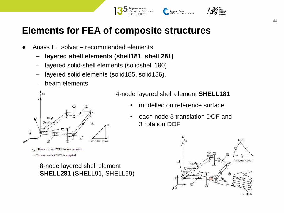
Elements for FEA of composite structures
● Ansys FE solver – recommended elements
– layered shell elements (shell181, shell 281)
– layered solid-shell elements (solidshell 190)
– layered solid elements (solid185, solid186),
– beam elements
8-node layered shell element
SHELL281 (SHELL91, SHELL99)
4-node layered shell element SHELL181
• modelled on reference surface
• each node 3 translation DOF and
3 rotation DOF
45
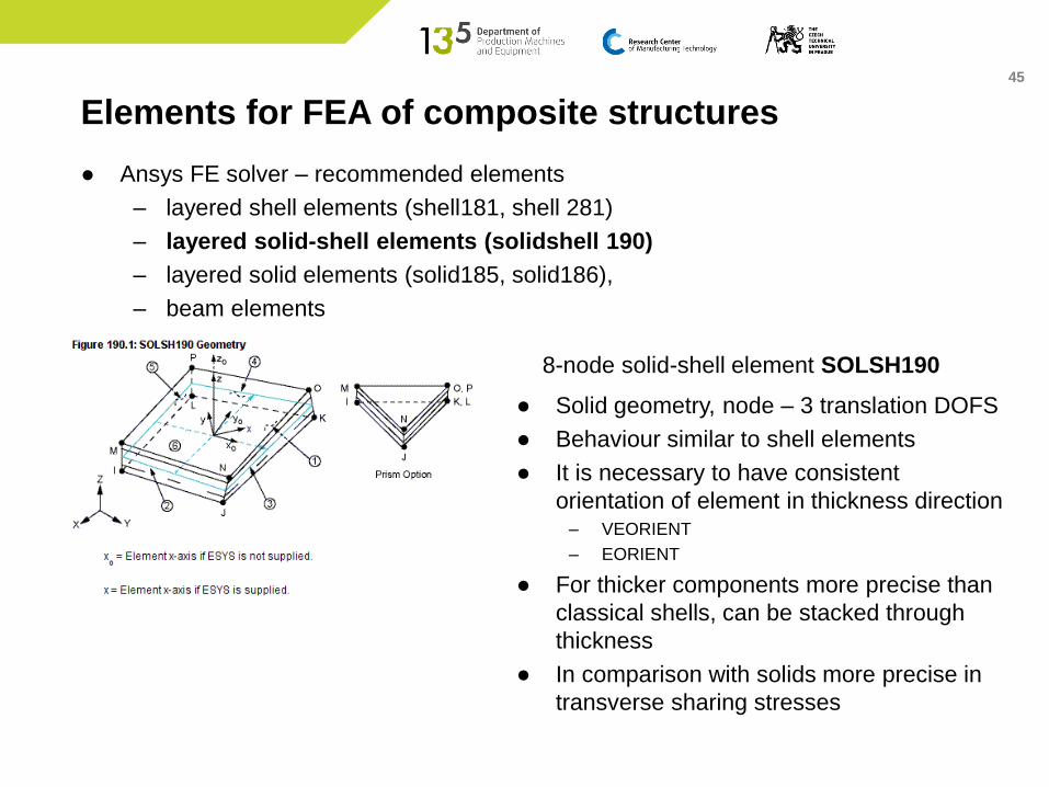
Elements for FEA of composite structures
● Ansys FE solver – recommended elements
– layered shell elements (shell181, shell 281)
– layered solid-shell elements (solidshell 190)
– layered solid elements (solid185, solid186),
– beam elements
● Solid geometry, node – 3 translation DOFS
● Behaviour similar to shell elements
● It is necessary to have consistent
orientation of element in thickness direction– VEORIENT
– EORIENT
● For thicker components more precise than
classical shells, can be stacked through
thickness
● In comparison with solids more precise in
transverse sharing stresses
8-node solid-shell element SOLSH190

46
Elements for FEA of composite structures
● Ansys FE solver – recommended elements
– layered shell elements (shell181, shell 281)
– layered solid-shell elements (solidshell 190)
– layered solid elements (solid185, solid186),
– beam elements
8-node layered solid element SOLID185
• limited usage (free edge
problems,…)
20-node layered solid element
SOLID186
47
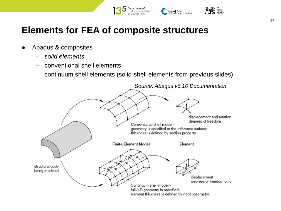
Elements for FEA of composite structures
● Abaqus & composites
– solid elements
– conventional shell elements
– continuum shell elements (solid-shell elements from previous slides)
Source: Abaqus v6.10 Documentation
48
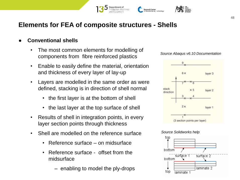
Elements for FEA of composite structures - Shells
● Conventional shells
• The most common elements for modelling of
components from fibre reinforced plastics
• Enable to easily define the material, orientation
and thickness of every layer of lay-up
• Layers are modelled in the same order as were
defined, stacking is in direction of shell normal
• the first layer is at the bottom of shell
• the last layer at the top surface of shell
• Results of shell in integration points, in every
layer section points through thickness
• Shell are modelled on the reference surface
• Reference surface – on midsurface
• Reference surface - offset from the
midsurface
– enabling to model the ply-drops
Source Abaqus v6.10 Documentation
Source Solidworks help
49
Elements for FEA of composite structures - Shells
● Basic assumptions for using shell elements
• each ply is modelled as homogenous, its thickness is significantly smaller in
comparison with the other dimensions
• interface between the layers is ideally rigid, thin, the displacements of the
layers through the interfaces are therefore continuous
• Kirchhof or First Order Shear Theory
• shell thickness does not change with deformation
• the ration of smallest dimension of shell surface to its thickness is larger than
10
• stiffness of laminate in coordinates X, Y, Z of shell does not differ by more
than 2 orders (might be violated in sandwich constructions)
• more:
http://mechanika2.fs.cvut.cz/old/pme/predmety/mkp1/podklady/skorepiny_ju.
50
Elements for FEA of composite structures - Shells
● Basic difference in comparison with modelling of isotropic materials
– Potential source of fatal errors if neglected
● Isotropic shells in commercial FE solvers
– default: data stored in the top and bottom layer of the shell
• maximum of bending stresses
• safe for evaluation of strength
● Orthotropic shells
– when using default settings without enhancing the data storage to every
layer
• layers with maximal loading might be not evaluated in terms of stress,
strain and failure
• only top and bottom layer post-processed
● Works both for conventional and continuum shells
– If you need to investigate the stress loading of component and potential
failure, you need to know the stress loading of every layer in critical area of
components
• If deformations are needed only, this can be neglected
51
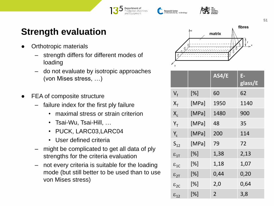
Strength evaluation
● Orthotropic materials
– strength differs for different modes of
loading
– do not evaluate by isotropic approaches
(von Mises stress, …)
● FEA of composite structure
– failure index for the first ply failure
• maximal stress or strain criterion
• Tsai-Wu, Tsai-Hill, …
• PUCK, LARC03,LARC04
• User defined criteria
– might be complicated to get all data of ply
strengths for the criteria evaluation
– not every criteria is suitable for the loading
mode (but still better to be used than to use
von Mises stress)
AS4/E E-glass/E
Vf [%] 60 62
XT [MPa] 1950 1140
Xc [MPa] 1480 900
YT [MPa] 48 35
Yc [MPa] 200 114
S12 [MPa] 79 72
1T [%] 1,38 2,13
1C [%] 1,18 1,07
2T [%] 0,44 0,20
2C [%] 2,0 0,64
12 [%] 2 3,8
52
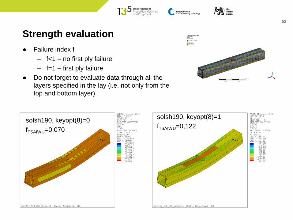
Strength evaluation
● Failure index f
– f<1 – no first ply failure
– f=1 – first ply failure
● Do not forget to evaluate data through all the
layers specified in the lay (i.e. not only from the
top and bottom layer)
solsh190, keyopt(8)=0
fTSAIWU=0,070
solsh190, keyopt(8)=1
fTSAIWU=0,122
53
Strength evaluation
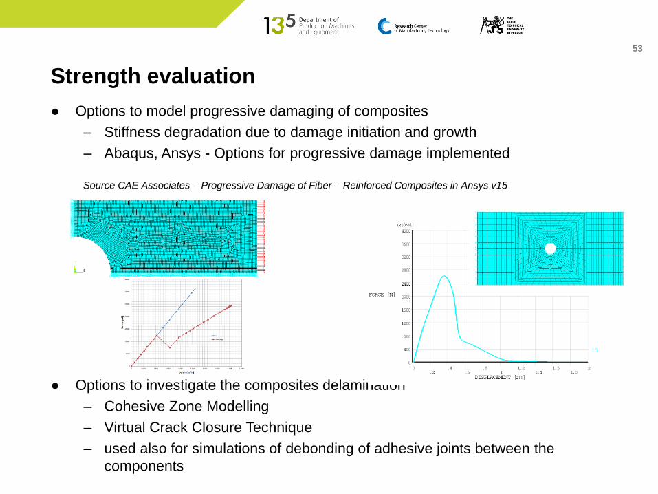
● Options to model progressive damaging of composites
– Stiffness degradation due to damage initiation and growth
– Abaqus, Ansys - Options for progressive damage implemented
● Options to investigate the composites delamination
– Cohesive Zone Modelling
– Virtual Crack Closure Technique
– used also for simulations of debonding of adhesive joints between the
components
Source CAE Associates – Progressive Damage of Fiber – Reinforced Composites in Ansys v15
54
Composite structures
● Short conclusions in terms of modelling – structural level
– Usually thin components (thickness is significantly smaller than other 2
dimensions)
• Suitable for shell elements, beam elements
• Options for solid modelling limited
– Usually composite lay-up with layers with multiangle orientations, structures
with only 1 orientation of fibres are rare
• Conventional shell elements
– definition of full composite lay-up
» material, thickness, orientation in respect to element normal
– specification by ABD matrix
» ABD matrix, optionally with transverse shear stiffness
– specification by homogenized properties
» modules of laminate
55
Composite structures
● Short conclusions in terms of modelling – structural level
– Usually thin components (thickness is significantly smaller than other 2
dimensions)
• Suitable for shell elements, beam elements
• Options for solid modelling limited
– Usually composite lay-up with layers with multiangle orientations, structures
with only 1 orientation of fibres are rare
• Continuum shell elements
– definition of full composite lay-up
» material, relative thickness, orientation in respect to element
normal
– specification by homogenized properties
» modules of laminate
– specification by ABD matrix not applicable
– must be divided into sub-laminates if having more than 1 element
through thickness

56
Composite structures
● Short conclusions in terms of modelling – structural level
– Usually thin components (thickness is significantly smaller than other 2
dimensions)
• Suitable for shell elements, beam elements
• Options for solid modelling limited
– Usually composite lay-up with layers with multiangle orientations, structures
with only 1 orientation of fibres are rare
• Continuum shell elements
– definition of full composite lay-up
» material, relative thickness, orientation in respect to element
normal
– specification by homogenized properties
» modules of laminate
– specification by ABD matrix not applicable
– must be divided into sub-laminates if having more than 1 element
through thickness
57
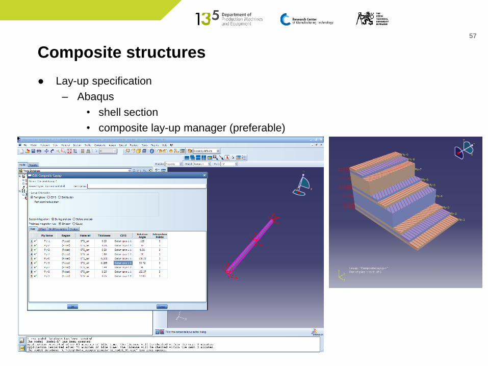
Composite structures
● Lay-up specification
– Abaqus
• shell section
• composite lay-up manager (preferable)
58
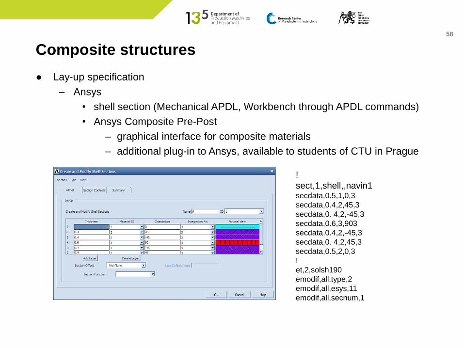
Composite structures
● Lay-up specification
– Ansys
• shell section (Mechanical APDL, Workbench through APDL commands)
• Ansys Composite Pre-Post
– graphical interface for composite materials
– additional plug-in to Ansys, available to students of CTU in Prague
!
sect,1,shell,,navin1 secdata,0.5,1,0,3
secdata,0.4,2,45,3
secdata,0. 4,2,-45,3
secdata,0.6,3,903
secdata,0.4,2,-45,3
secdata,0. 4,2,45,3
secdata,0.5,2,0,3
!
et,2,solsh190
emodif,all,type,2
emodif,all,esys,11
emodif,all,secnum,1
59
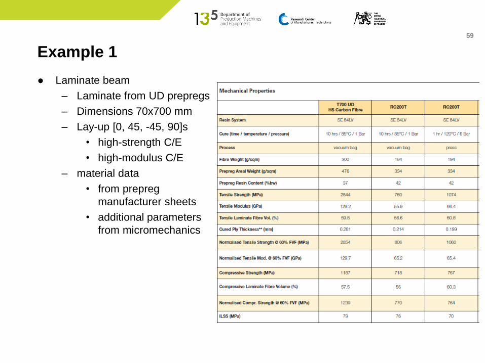
Example 1
● Laminate beam
– Laminate from UD prepregs
– Dimensions 70x700 mm
– Lay-up [0, 45, -45, 90]s
• high-strength C/E
• high-modulus C/E
– material data
• from prepreg
manufacturer sheets
• additional parameters
from micromechanics
60
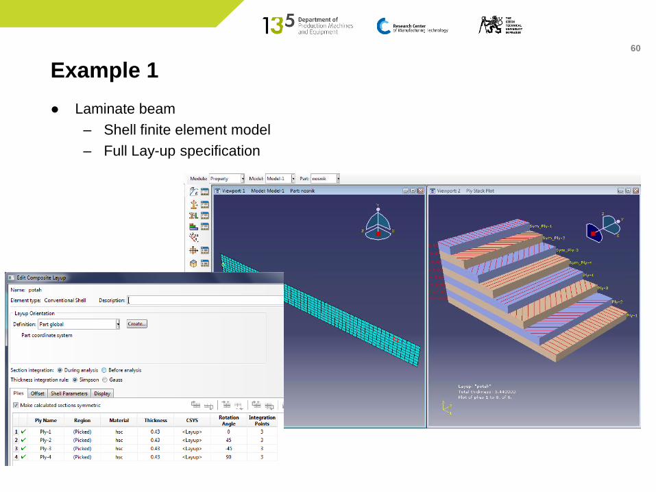
Example 1
● Laminate beam
– Shell finite element model
– Full Lay-up specification

61
Example 1
● Comparison with experimental results
– modal analysis
• mode shapes and its frequencies
• match between FE and experiment acceptable
Mode [-] Experiment
[Hz]
FEA
[Hz]
1 42.5 46.4
2 121.5 132.6
3 193.5 206.2
4 242.4 266.4
5 406.2 419.4
Mass [g] 262.5 263.8
62
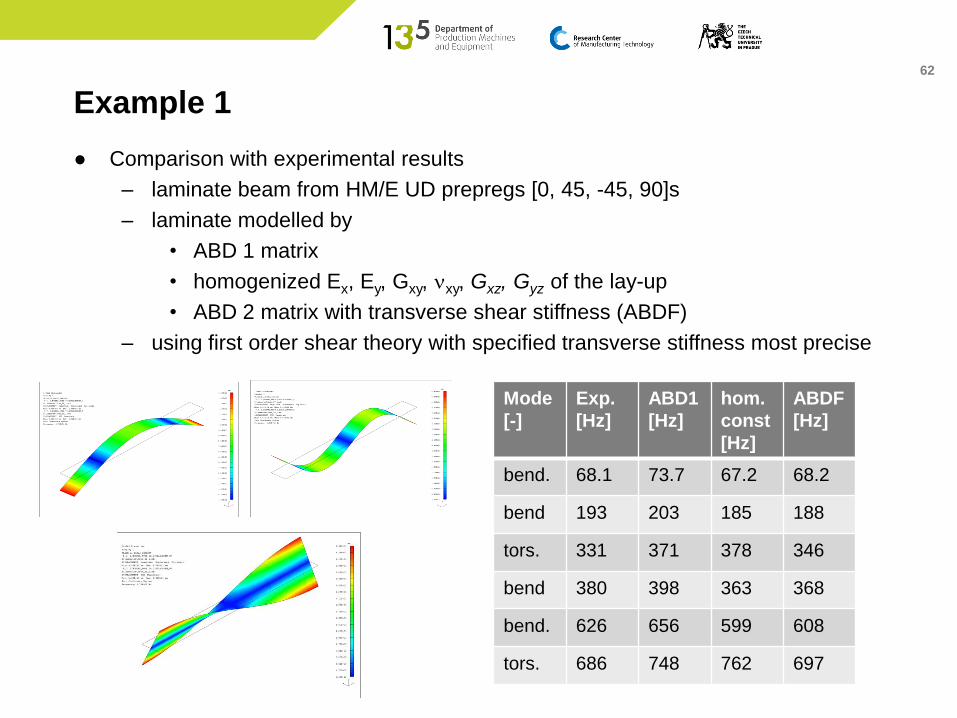
Example 1
● Comparison with experimental results
– laminate beam from HM/E UD prepregs [0, 45, -45, 90]s
– laminate modelled by
• ABD 1 matrix
• homogenized Ex, Ey, Gxy, nxy, Gxz, Gyz of the lay-up
• ABD 2 matrix with transverse shear stiffness (ABDF)
– using first order shear theory with specified transverse stiffness most precise
Mode
[-]
Exp.
[Hz]
ABD1
[Hz]
hom.
const
[Hz]
ABDF
[Hz]
bend. 68.1 73.7 67.2 68.2
bend 193 203 185 188
tors. 331 371 378 346
bend 380 398 363 368
bend. 626 656 599 608
tors. 686 748 762 697
63
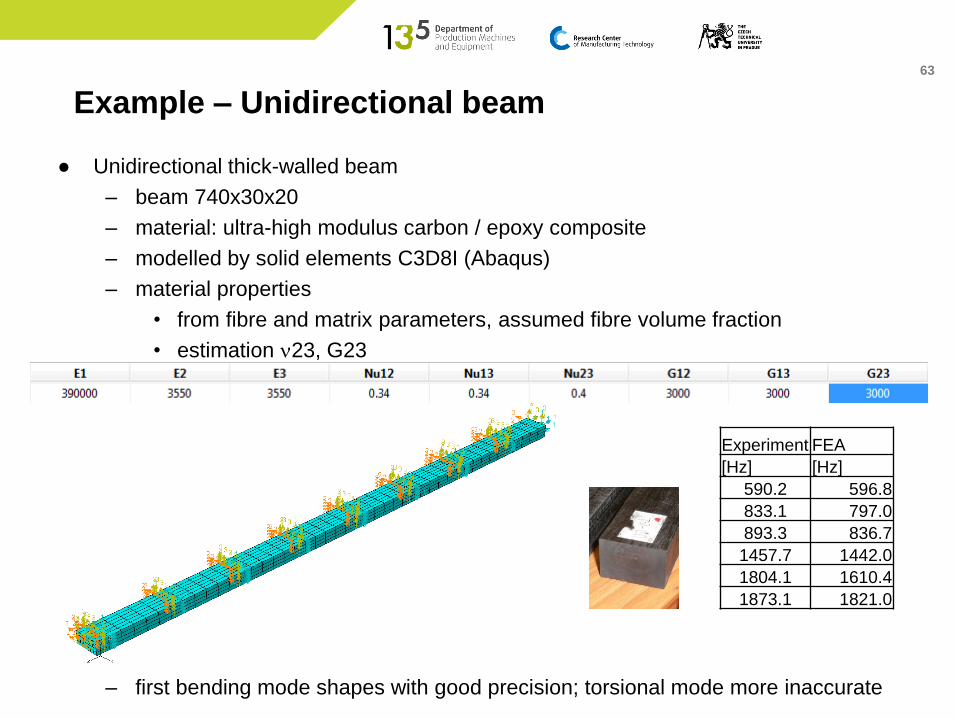
Example – Unidirectional beam
● Unidirectional thick-walled beam
– beam 740x30x20
– material: ultra-high modulus carbon / epoxy composite
– modelled by solid elements C3D8I (Abaqus)
– material properties
• from fibre and matrix parameters, assumed fibre volume fraction
• estimation n23, G23
– first bending mode shapes with good precision; torsional mode more inaccurate
Experiment FEA
[Hz] [Hz]
590.2 596.8
833.1 797.0
893.3 836.7
1457.7 1442.0
1804.1 1610.4
1873.1 1821.0
64
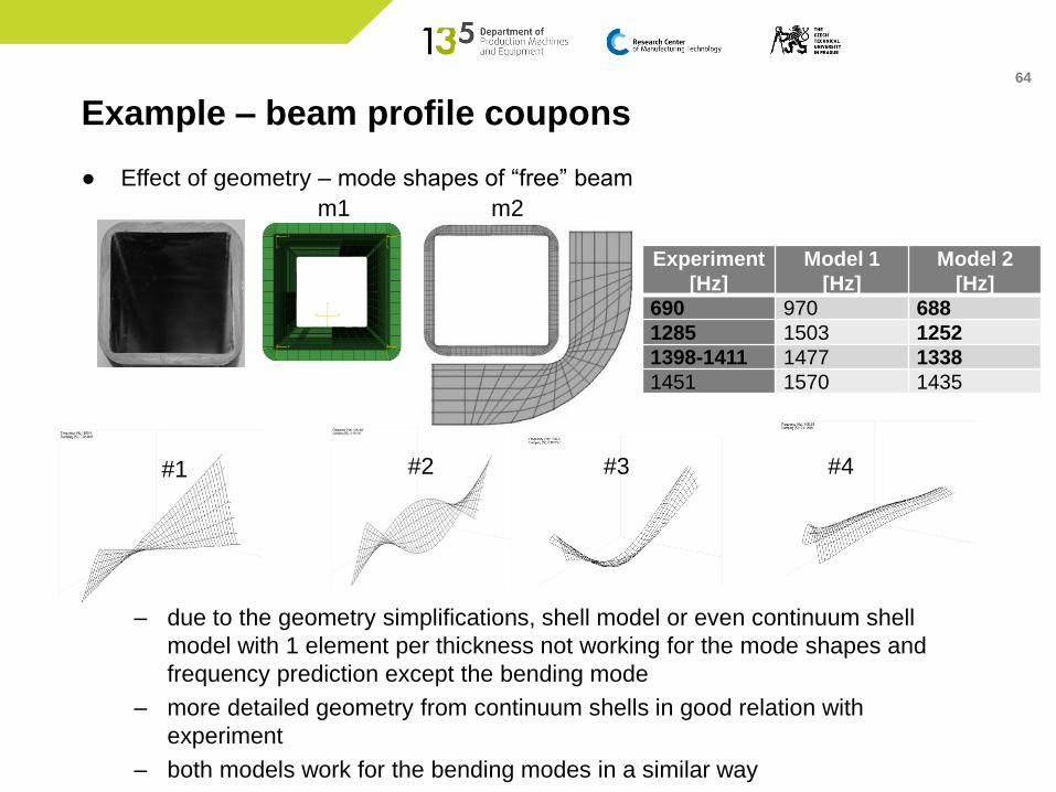
Example – beam profile coupons
● Effect of geometry – mode shapes of “free” beam
– due to the geometry simplifications, shell model or even continuum shell
model with 1 element per thickness not working for the mode shapes and
frequency prediction except the bending mode
– more detailed geometry from continuum shells in good relation with
experiment
– both models work for the bending modes in a similar way
Experiment
[Hz]
Model 1
[Hz]
Model 2
[Hz]
690 970 688
1285 1503 1252
1398-1411 1477 1338
1451 1570 1435
#1 #2 #3 #4
m1 m2
65
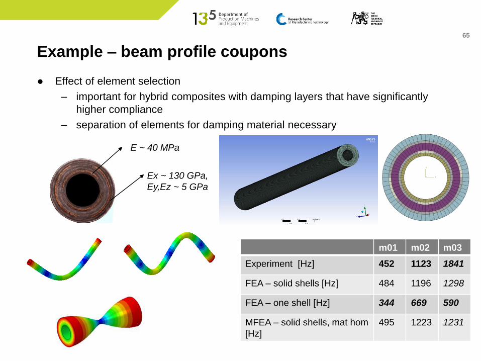
Example – beam profile coupons
● Effect of element selection
– important for hybrid composites with damping layers that have significantly
higher compliance
– separation of elements for damping material necessary
E ~ 40 MPa
Ex ~ 130 GPa,
Ey,Ez ~ 5 GPa
m01 m02 m03
Experiment [Hz] 452 1123 1841
FEA – solid shells [Hz] 484 1196 1298
FEA – one shell [Hz] 344 669 590
MFEA – solid shells, mat hom
[Hz]
495 1223 1231
66
Example – beam profile coupons
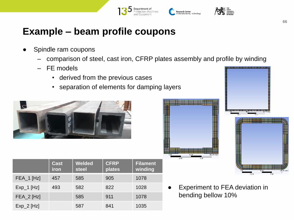
● Spindle ram coupons
– comparison of steel, cast iron, CFRP plates assembly and profile by winding
– FE models
• derived from the previous cases
• separation of elements for damping layers
Cast
iron
Welded
steel
CFRP
plates
Filament
winding
FEA_1 [Hz] 457 585 905 1078
Exp_1 [Hz] 493 582 822 1028
FEA_2 [Hz] 585 911 1078
Exp_2 [Hz] 587 841 1035
● Experiment to FEA deviation in
bending bellow 10%

67
Example - hybrid spindle ram
● Modelling of hybrid spindle ram and
its composite reinforcement
– Combination of carbon/epoxy
layers from PITCH and PAN fibres,
1 integrated damping layer
– Solid shell model with element
stacking
– For bending modes deviation
between FEA and experiment
bellow 5%
– For other modes deviation up to
20% and more
Mode [-] fEXP [Hz] fFEA [Hz] DfFEA/EXP [%]
1 492 468 -4,9 1st bending2 493 596 20,93 784 715 -8,84 922 921 -0,15 1 158 1 124 -2,9 2nd bending
#1 #2 #3 #4
68
Example – material degradation
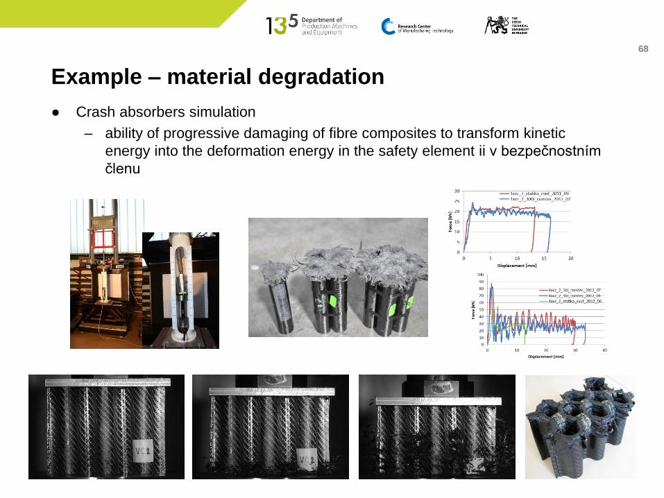
● Crash absorbers simulation
– ability of progressive damaging of fibre composites to transform kinetic
energy into the deformation energy in the safety element ii v bezpečnostním
členu

69
● Simulations of progressive damaging
– progressive damage implemented by failure criteria (Chang-Chang)
• element stiffness degradation in respect to achieving criterion
• after the set level of degradation – element removal
– Chang-Chang failure criterion
• fibre failure in tension stiffness change of element for fft=1
• fibre failure in compression stiffness change of element for ffc=1
• matrix failure in tension stiffness change of element for fmt=1
• matrix failure in compression stiffness change of element for fmc=1
Example – material degradation
,10,ˆˆ
2
12
2
11
s
swhere
SXf
LTft𝐸11 = 𝐸22 = 𝐺12 = 𝜈12 = 𝜈21 = 0
,ˆ
2
11
CfcX
fs
,ˆˆ
2
12
2
22
LTmtSY
fss
.ˆˆ
122
ˆ2
1222
22
22
LCT
C
TmcSYS
Y
Sf
sss
𝐸11 = 𝜈12 = 𝜈21 = 0,
𝐸22 = 𝐺12 = 𝜈21 = 0,
𝐸22 = 𝐺12 = 𝜈12 = 𝜈21 = 0
70
Example – material degradation
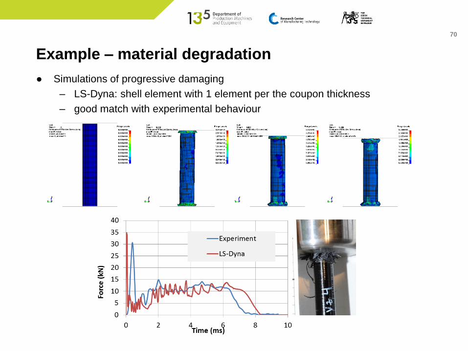
● Simulations of progressive damaging
– LS-Dyna: shell element with 1 element per the coupon thickness
– good match with experimental behaviour

71
Example – material degradation
● Simulations of progressive damaging
72
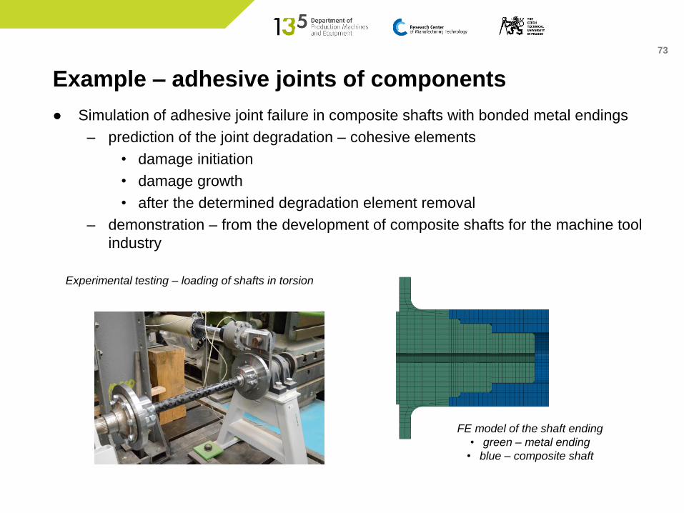
Example – adhesive joints of components
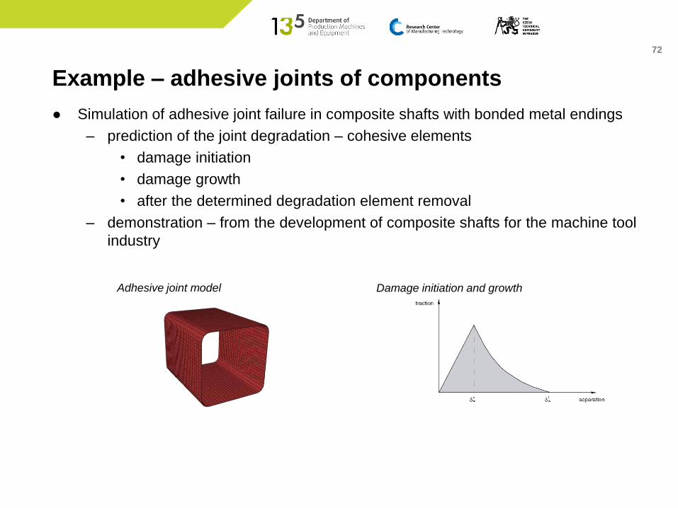
● Simulation of adhesive joint failure in composite shafts with bonded metal endings
– prediction of the joint degradation – cohesive elements
• damage initiation
• damage growth
• after the determined degradation element removal
– demonstration – from the development of composite shafts for the machine tool
industry
Damage initiation and growthAdhesive joint model
73
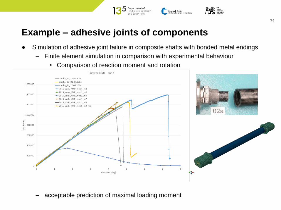
Example – adhesive joints of components
● Simulation of adhesive joint failure in composite shafts with bonded metal endings
– prediction of the joint degradation – cohesive elements
• damage initiation
• damage growth
• after the determined degradation element removal
– demonstration – from the development of composite shafts for the machine tool
industry
Experimental testing – loading of shafts in torsion
FE model of the shaft ending
• green – metal ending
• blue – composite shaft
74
Example – adhesive joints of components
● Simulation of adhesive joint failure in composite shafts with bonded metal endings
– Finite element simulation in comparison with experimental behaviour
• Comparison of reaction moment and rotation
– acceptable prediction of maximal loading moment
75
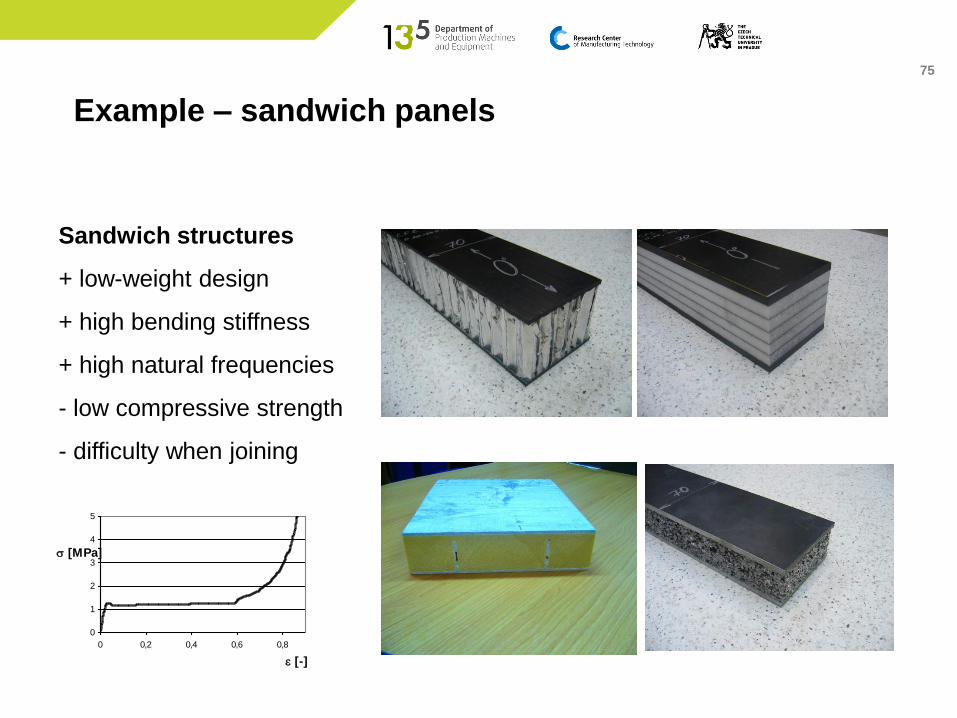
Sandwich structures
+ low-weight design
+ high bending stiffness
+ high natural frequencies
- low compressive strength
- difficulty when joining
0
1
2
3
4
5
0 0,2 0,4 0,6 0,8
[-]
s [MPa]
Example – sandwich panels

76
Necessary to include the effect of transverse shearing
FEA
• due to transverse shearing, the normal to the reference surface rotates
• shell element cannot behave in this way
• with some exceptions (sandwich logic, balance of energy)
Ansys:
• Shell91 – former element for sandwich simulations
• nowadays Shell181,281 - elements model the transverse-
shear deflection using an energy-equivalence method
Example – sandwich panels

77
Approaches for FE modelling of sandwich panels
Shell elements
- generally care must be taken as the approach of using 1 shell element for the sandwich
structure might work only for specified shells in one FE solver, but not in other solver
- problematic behaviour of the core with larger compliance (stiffness is lower by 3 orders
in comparison with skins – does not meet the conditions for shells)
Solid elements
- core and skins modelled by solid elements, or solid-shell elements
- might be problematic for composite skins
Combination of solid and shell elements
- core modelled by solid elements
- skins modelled by shell or solid shell elements
Example – sandwich panels
78
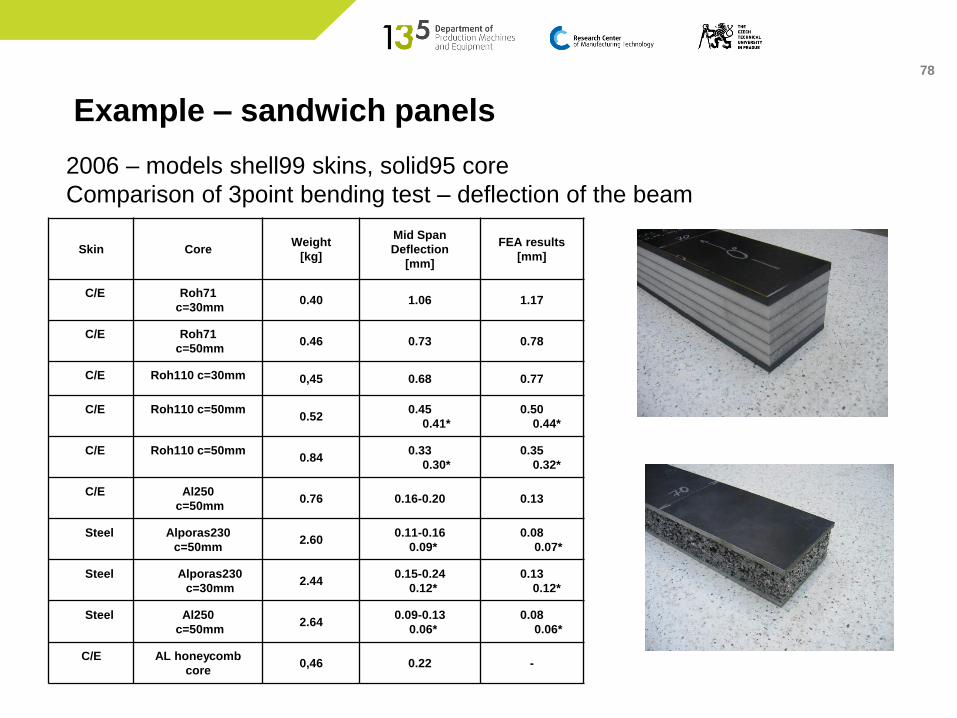
Skin CoreWeight
[kg]
Mid Span
Deflection
[mm]
FEA results
[mm]
C/E Roh71
c=30mm0.40 1.06 1.17
C/E Roh71
c=50mm0.46 0.73 0.78
C/E Roh110 c=30mm 0,45 0.68 0.77
C/E Roh110 c=50mm0.52
0.45
0.41*
0.50
0.44*
C/E Roh110 c=50mm0.84
0.33
0.30*
0.35
0.32*
C/E Al250
c=50mm0.76 0.16-0.20 0.13
Steel Alporas230
c=50mm2.60
0.11-0.16
0.09*
0.08
0.07*
Steel Alporas230
c=30mm2.44
0.15-0.24
0.12*
0.13
0.12*
Steel Al250
c=50mm2.64
0.09-0.13
0.06*
0.08
0.06*
C/E AL honeycomb
core0,46 0.22 -
2006 – models shell99 skins, solid95 core
Comparison of 3point bending test – deflection of the beam
Example – sandwich panels
79
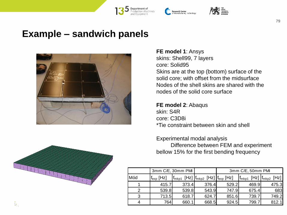
Mód fexp [Hz] fmkp1 [Hz] fmkp2 [Hz] fexp [Hz] fmkp1 [Hz] fmkp2 [Hz]
1 415.7 373.4 376.4 529.2 469.9 475.3
2 539.8 539.8 543.9 747.9 675.4 683
3 713.5 618.7 624.7 851.6 739.7 749.2
4 764 660.1 668.5 924.5 799.7 812.1
3mm C/E, 30mm PMI 3mm C/E, 50mm PMI
FE model 1: Ansys
skins: Shell99, 7 layers
core: Solid95
Skins are at the top (bottom) surface of the
solid core; with offset from the midsurface
Nodes of the shell skins are shared with the
nodes of the solid core surface
FE model 2: Abaqus
skin: S4R
core: C3D8i
*Tie constraint between skin and shell
Experimental modal analysis
Difference between FEM and experiment
bellow 15% for the first bending frequency
Example – sandwich panels