Chapter 3

Finite Difference Methods

3.1 Notations

Remark 3.1 Idea. The basic idea of finite difference methods consists in approxi-mating the derivatives of a differential equation with appropriate finite differences.Consider a decomposition of the interval [0, 1], which is at the moment assumed tobe equidistant:

xi = ih, i = 0, . . . , N, h = 1/N,

ωh = xi : i = 0, . . . , N – grid, mesh.

2

Definition 3.2 Grid function. A vector uh = (u0, . . . , uN )T ∈ RN+1, which

assigns to each grid point (node) a value is called grid function. The restriction ofa function u ∈ C([0, 1]) to a grid function is denoted by Rhu, i.e.,

Rhu := (u(x0), u(x1), . . . , u(xN ))T.

2

Example 3.3 Grid function. Consider a grid with the nodes 0, 0.25, 0.5, 0.75, 1.Then, the grid function of u(x) = x2 is

Rhu =

(

0,1

16,1

4,9

16, 1

)T

.

Different functions might have for a given grid the same grid function. Consider,e.g., u(x) = sin(4πx) on the same grid as used above. The corresponding gridfunction is

Rhu = (0, 0, 0, 0, 0)T.

This grid function is obviously also the grid function of u(x) = 0. The consideredgrid is too coarse to represent the u(x) = sin(4πx) in a reasonable way. 2

Definition 3.4 Finite difference operators. Let v(x) be a sufficiently smoothfunction and denote vi = v(xi), where xi are the nodes of the grid. The followingdifference quotients (finite differences) are called

D+v(xi) = vx,i =vi+1 − vi

h– forward difference,

D−v(xi) = vx,i =vi − vi−1

h– backward difference,

D0v(xi) = vx,i =vi+1 − vi−1

2h– central difference,

D+D−(v)(xi) = vxx,i =vi+1 − 2vi + vi−1

h2– second order difference,

19

see Figure 3.1. 2

Figure 3.1: Finite differences.

Remark 3.5 To the finite differences. The formula for D+D−(v)(xi) can bechecked with a direct calculation. In addition, it is

D0v(xi) =1

2

(

(D+v(xi) +D−v(xi))

.

2

Definition 3.6 Consistency of a finite difference operator, discrete max-

imum norm. Let L be a differential operator. The finite difference operatorLh : R

N+1 → RN+1 is said to be consistent with L of order k if

max0≤i≤N

|(Lu)(xi)− (Lhuh)i| =: ‖Lu− Lhuh‖∞,d = O(hk).

Here, ‖·‖∞,d is the discrete maximum norm in the space of grid functions. 2

Example 3.7 Orders of consistency for standard finite difference operators. Theconsistency is a measure of the approximation property of Lh. Applying a Taylorseries expansion for v(x) at the node xi yields

D+v(xi) = v′(xi) +O(h),

D−v(xi) = v′(xi) +O(h),

D0v(xi) = v′(xi) +O(h2),

D+D−(v)(xi) = v′′(xi) +O(h2).

The finite difference operators D+v(xi), D−v(xi), D

0v(xi) are consistent to L =ddx of first, first, and second order, respectively. The operator D+D−(v)(xi) is

consistent of second order to L = d2

dx2 . 2

20

Figure 3.2: Brook Taylor (1685 – 1731).

3.2 Classical Convergence Theory for Central Dif-

ference Schemes

Remark 3.8 Contents of this section. This section considers the two-point bound-ary value problem

Lu := −u′′ + b(x)u′ + c(x)u = f(x), for x ∈ (0, 1), u(0) = u(1) = 0, (3.1)

i.e., the model problem with ε = 1. The classical convergence theory will be pre-sented. It will be assumed that the parameter functions b, c, f are sufficiently smoothand that c(x) ≥ 0 for all x ∈ [0, 1]. 2

Definition 3.9 Central difference scheme. The central difference scheme for(3.1) has the form

(Lhuh)i := −D+D−ui + biD0ui + ciui = fi, for i = 1, . . . , N − 1,

u0 = uN = 0. (3.2)

2

Remark 3.10 To the central difference scheme.

• The central difference scheme leads to a tridiagonal system of linear equations

riui−1 + siui + tiui+1 = fi, i = 1, . . . , N − 1, u0 = uN = 0,

with

ri = −1

h2−

1

2hbi, si = ci +

2

h2, ti = −

1

h2+

1

2hbi.

• The following questions have to be answered:

Which properties has the discrete problem (3.2)? What can be said about the error ‖u− uh‖∞,d?

For answering these questions, the concepts of consistency and stability will beused.

2

21

Definition 3.11 Consistency of a difference scheme and order of consis-

tency. Consider a difference scheme of the form Lhuh := Rh(Lu). The boundaryconditions should be integrated into this scheme such that the first and last row of Lh

are identical to the first and last row of the identity matrix and it is Rh(Lu)0 = u0,Rh(Lu)N = uN . The scheme is called consistent of order k in the discrete maximumnorm, if

‖LhRhu−Rh(Lu)‖∞,d ≤ chk,

where the positive constants c and k are independent of h. 2

Lemma 3.12 Consistency order of the central difference scheme. Assume

that u ∈ C4([0, 1]), then the central difference scheme (3.2) has consistency order 2.

Proof: The proof uses a Taylor series expansion, exercise.

Definition 3.13 Stability of a difference scheme. A difference scheme Lhuh =fh is called stable in the discrete maximum norm, if there is a stability constant cS ,which is independent of h, with

‖uh‖∞,d ≤ cS ‖Lhuh‖∞,d = cS ‖fh‖∞,d

for all grid functions uh. 2

Definition 3.14 Convergence of a difference scheme and order of con-

vergence. A difference scheme for (3.1) is convergent of order k in the discretemaximum norm, if there are positive constants c and k, which are independent ofh, such that

‖uh −Rhu‖∞,d ≤ chk.

2

Theorem 3.15 Consistency + stability =⇒ convergence. A consistent and

stable difference scheme is convergent. The orders of consistency and convergence

are the same.

Proof: It is

‖uh −Rhu‖∞,d

stab.

≤ cS ‖Lh (uh −Rhu)‖∞,d

lin.= cS ‖Lhuh − LhRhu‖∞,d

= cS ‖fh − LhRhu‖∞,d= cS ‖Rhf − LhRhu‖∞,d

= cS ‖RhLu− LhRhu‖∞,d

cons.

≤ Khk,

where the constant K is the product of the constants from the stability and consistency

condition.

Remark 3.16 To consistency and stability. One has to prove consistency andstability.

• Consistency proofs are based often on Taylor series expansions and they areperformed in a standard way.

• Stability proofs are not performed only at functions but they are performed atmatrices and functions, see Definition 3.13. They are generally not simple andthey require the introduction of some new notations.

2

22

Definition 3.17 Natural order of vectors and matrices, inverse-monotone

matrices. Let x,y ∈ Rn. Then one writes x ≤ y if and only if xi ≤ yi for

all i = 1, . . . , n. The notation x ≥ 1 means that xi ≥ 1 for all i = 1, . . . , n.Analogously, the notation A ≥ 0 means for a matrix A = (aij) ∈ R

n×n that aij ≥ 0for all i, j = 1, . . . , n.

A matrix A, for which the inverse A−1 exists with A−1 ≥ 0 is called inverse-monotone matrix. 2

Lemma 3.18 Discrete comparison principle. Let A ∈ Rn×n be inverse-mono-

tone. If Av ≤ Aw for v,w ∈ Rn, then it follows that v ≤ w.

Proof: From the assumption, it follows that

A(v −w) := b ≤ 0.

Multiplication with A−1 givesv −w = A−1

b ≤ 0.

The last inequality follows from the property that A is an inverse-monotone matrix. Non-

negative matrix entries are multiplied with nonpositive vector entries of b. The result is

a vector with nonpositive components.

Remark 3.19 To Lemma 3.18. Lemma 3.18 is a discrete analog to the comparisonprinciple from Corollary 2.34. 2

Definition 3.20 M-matrix. A matrix A = (aij) ∈ Rn×n is called an M-matrix,

if:

1. aij ≤ 0 for i 6= j,2. A−1 exists with A−1 ≥ 0.

2

Lemma 3.21 M-matrices have positive diagonal entries. Let A = (aij) ∈R

n×n be an M-matrix, then it is aii > 0, i = 1, . . . , n.

Proof: Exercise.

Remark 3.22 On M-matrices. M-matrices are an important subclass of inverse-monotone matrices, which will become very useful in the analysis. However, inpractice, the second condition of their definition is hard to check. But there arecharacterizations of M-matrices which are easier to check.

Then name refers to Hermann Minkowski. 2

Theorem 3.23 M-matrix criterion. Let A = (aij) ∈ Rn×n with aij ≤ 0 for

i 6= j. Then A is an M-matrix if and only if there exists a vector e ∈ Rn, e > 0,

such that Ae > 0. In this case, one obtains for the row sum norm

∥

∥A−1∥

∥

∞≤

‖e‖∞,d

mink (Ae)k. (3.3)

The vector e is called majorizing element.

Proof: See the literature, e.g., Bohl (1981); Axelsson and Kolotilina (1990).

Remark 3.24 Concerning the M-matrix criterion.

23

• The following approach is often successful for the construction of a majorizingelement.

Find a function e(x) > 0 such that (Le)(x) > 0 for x ∈ (0, 1). This functionis a majorizing element of the differential operator L.

Restrict e(x) to its corresponding grid function eh.

If the first step of this approach is possible and the discretization Lh of L isconsistent, then this approach generally works, at least if the mesh width issufficiently small. The matrix A is the matrix representation of Lh.

• The constant cS in the definition of the stability can be estimated with (3.3)

‖uh‖∞,d =∥

∥A−1fh∥

∥

∞,d≤

∥

∥A−1∥

∥

∞‖fh‖∞,d =

∥

∥A−1∥

∥

∞‖Lhuh‖∞,d .

Hence, it holds for this constant

cS ≤‖e‖∞,d

mink (Ae)k.

Thus, from the M-matrix criterion, which is equivalent to the M-matrix property,it follows stability.

• If Dirichlet boundary conditions are prescribed, then the variables u0 and uN

should be eliminated before Theorem 3.23 is applied.• For the central finite difference scheme, the first requirement of the M-matrixcriterion, aij ≤ 0 for i 6= j, is satisfied if h is sufficiently small, see Remark 3.10for the coefficients of the matrix.

2

Example 3.25 M-matrix criterion. Consider (3.1) with b(x) ≡ 0, i.e.,

Lu(x) = −u′′(x) + c(x)u(x), u(0) = u(1) = 0, c(x) ≥ 0 in [0, 1].

Choose e(x) := 12x(1− x), then it follows that

Le(x) = 1 + c(x)e(x) ≥ 1.

Setting eh := Rhe gives for all nodes xi

(Lheh)i = −D+D−eh,i + cieh,i = 1 + cieh,i ≥ 1,

because the second order finite difference discretizes the second derivative of aquadratic function in the interior nodes exactly, see Example 3.7. One gets

Lheh ≥ (1, . . . , 1)T

⇐⇒ Ae ≥ 1.

As bound for the stability constant, one obtains

cS ≤‖e‖∞,d

mink (Ae)k≤

eh(1/2)

1=

1/8

1=

1

8.

This example shows that in the case b(x) ≡ 0 the M-matrix property holdswithout restrictions on the fineness of the grid. 2

Lemma 3.26 Stability of the central finite difference scheme for suffi-

ciently fine grids. If the mesh width h is sufficiently small, then the central finite

difference scheme (3.2) for the two-point boundary value problem (3.1) is stable in

the discrete maximum norm. The stiffness matrix is an M-matrix.

24

Proof: A majorizing element will be constructed. To this end, let e(x) be the solutionof the two-point boundary value problem

−e′′ + b(x)e′ = 1, e(0) = e(1) = 0.

From the maximum principle, Lemma 2.31, it follows that e(x) ≥ 0 for x ∈ (0, 1). Inaddition, e(x) has no local minima in (0, 1) since in this case, one obtains from the equationthat −e′′(x) = 1 for the local minima, which is a contradiction. Since e(x) 6≡ 0, it ise(x) > 0 for x ∈ (0, 1). Since c(x) ≡ 0, one gets with Corollary 2.39 that the givenproblem possesses a unique solution and that e ∈ C([0, 1]). Hence, e(x) is bounded. Byconstruction, it is

Le(x) = −e′′(x) + b(x)e′(x) + c(x)e(x) = 1 + c(x)e(x).

Let eh be the grid function of e(x). For interior nodes, one obtains with c(x) ≥ 0

(Lheh)i = (RhLe)i + (Lheh −RhLe)i

= (Rh (1 + c(x)e(x)))i+(

−D+D−eh + biD0eh + cieh − 1− cieh

)

i

≥ 1 +(

−D+D−eh + biD0eh − 1

)

i

=(

−D+D−eh + biD0eh)

i.

Since eh is the grid function that corresponds to e(x), the expression in the last lineapproximates −e′′(xi) + b(xi)e

′(xi)(= 1) sufficiently well, if h sufficiently small, see theconsistency estimate in Example 3.7. In particular, there is a H > 0 such that for allh ∈ (0, H] it is

(Lheh)i ≥1

2.

Now, the proof of the theorem is finished with the application of the M-matrix criterion

and using the property that aij ≤ 0 for sufficiently fine meshes.

Corollary 3.27 Second order convergence of the central difference scheme.

If u ∈ C4([0, 1]), then the central difference scheme (3.2) is convergent with second

order.

Proof: The statement follows with Theorem 3.15 by combining Lemma 3.12 and

Lemma 3.26.

Example 3.28 Second order convergence of the central difference scheme for suf-

ficiently fine meshes. Consider the two-point boundary value problem

−u′′(x) + 2u′(x) + 3u(x) = 1 in (0, 1), u(0) = u(1) = 0.

The solution of this problem is

u(x) =1

3

(

1 +1− e−1

e−1 − e3e3x +

e3 − 1

e−1 − e3e−x

)

.

One obtains the following errors for different mesh widths

no. of intervals N ‖u− uh‖∞,d

4 4.2388e-48 9.8811e-516 2.4529e-532 6.1537e-664 1.5368e-6128 3.8440e-7256 9.6093e-8512 2.4023e-8

1024 6.0058e-9

It can be observed that the error is reduced by the factor four if the mesh width isreduced by the factor two. This behavior is second order convergence. 2

25

3.3 Upwind Schemes

Remark 3.29 Singularly perturbed two-point boundary value problem. From nowon, finite difference schemes will be studied for the two-point boundary value prob-lem

Lu := −εu′′ + b(x)u′ + c(x)u = f(x), for x ∈ (0, 1), (3.4)

with the boundary conditions

u(0) = u(1) = 0, (3.5)

and the assumptions

ε > 0,

b(x) > 0 for all x ∈ [0, 1],

c(x) ≥ 0 for all x ∈ [0, 1],

with sufficiently smooth functions b(x), c(x), and f(x). This problem is called sin-gularly perturbed if ε ‖b‖L∞(Ω). The parameter ε is called singular perturbation

parameter. With respect to the convection, it is only important that b(x) 6= 0 forall x ∈ [0, 1]. If b(x) < 0 in [0, 1], then one obtains a problem of form (3.4) byapplying the variable transform x 7→ 1− x.

If ε is small, then the solution of (3.4), (3.5) has in general a boundary layer atx = 1, see Example 2.8. This layer influences both the stability and the consistencyof the numerical method. If the boundary values are chosen such that there is noboundary layer, then the consistency improves but the stability of the method mightbe still a problem. 2

Example 3.30 Application of the central difference scheme to a simplified singu-

larly perturbed problem. Consider the problem

−εu′′ + u′ = 0 in (0, 1), u(0) = 0, u(1) = 1.

The solution of this problem is

u(x) =e−(1−x)/ε − e−1/ε

1− e−1/ε.

Applying the transform u(x) := x + v(x), one gets a problem with homogeneousboundary conditions. But one can apply the difference scheme directly to the prob-lem with inhomogeneous boundary conditions. This approach is used in practice.The discrete problem has the form

−εD+D−ui +D0ui = 0, u0 = 0, uN = 1

and it has the solution (exercise)

ui =ri − 1

rN − 1with r =

2ε+ h

2ε− h.

In particular, it is |r| > 1, since the numerator is the sum of two positive numbers.The absolute value of this sum is always larger than the absolute value of thedifference of these numbers.

If h 2ε then it is r ≈ −1 and it follows that

ui ≈(−1)i − 1

(−1)N − 1.

26

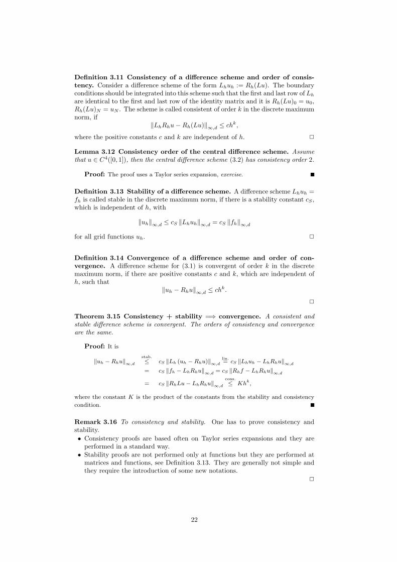
Figure 3.3: Solution (left) and discrete solution with the central difference scheme(right) for ε = 10−6 and h = 1/32.

If N even, then one divides by a very small positive number, since |r| > 1. For ieven, the numerator is also small and it is positive. Hence, the quotient is positive,too. For i odd, the numerator is negative and of order −2. In this case, the quotientis negative and its absolute value is large. The discrete solution is highly oscillating,see Figure 3.3.

If h < 2ε, then one obtains with the central difference scheme a useful approxi-mation of the solution. However, in applications it is often ε ≤ 10−6, i.e., one needsvery fine grids in order to apply the central difference scheme. The use of such gridsis possible in one dimension, but not in two or three dimensions. 2

Remark 3.31 Application of the central difference scheme to the general singularly

perturbed problem. Consider now the singularly perturbed problem (3.4), (3.5) andwrite the difference scheme in the form presented in Remark 3.10

riui−1 + siui + tiui+1 = fi, i = 1, . . . , N − 1, u0 = uN = 0,

with

ri = −ε

h2−

1

2hbi, si = ci +

2ε

h2, ti = −

ε

h2+

1

2hbi, bi > 0.

One obtains an M-matrix, and hence stability, if one assumes that

ti ≤ 0 =⇒ h ≤ h0(ε) =2ε

‖b‖∞.

This assumption generalizes the observation from Example 3.30. Note that h0(ε) →0 for ε → 0. 2

Remark 3.32 Motivation for upwind schemes. Another heuristic explanation forthe failure of the central difference scheme in the case ε h is as follows. For smallε, the method applied to Example 3.30 has essentially the form

D0ui = 0, ⇐⇒ui+1 − ui−1

2h= 0.

It follows for i = N − 1 that uN−2 ≈ uN = 1, which is a very bad approximation ofthe exact value u(xN−2) ≈ 0.

This observations leads to the idea that for the approximation of u′(xN−1) it isbetter not to use the value uN . The simplest candidate which has this feature isthe backward difference

u′(xi) ≈ui − ui−1

h.

27

If one has the goal to modify the matrix entries which are obtained with the centraldifference scheme in such a way that one gets an M-matrix, i.e., ti ≤ 0, then onecan also motivate backward difference approximation of the first derivative, becausethis condition is satisfied at any rate if for the discretization of the convective terma contribution from the node xi+1 is not used. 2

Definition 3.33 Simple upwind scheme. The simple upwind scheme for thesingularly perturbed two-point boundary value problem (3.4), (3.5) has the form

− εD+D−ui + biDNui + ciui = fi, for i = 1, . . . , N − 1,

u0 = uN = 0, (3.6)

with

DN :=

D+ for b < 0,D− for b > 0.

2

Remark 3.34 Concerning the simple upwind scheme.

• In the upwind scheme, the finite difference approximation of the convective termis computed with values from the upwind direction. For convection-dominatedproblems, the transport of information occurs in the direction of convection.Hence, the upwind direction is the direction from which information is coming.

• Using the simple upwind scheme, one obtains a much better numerical solutionfor Example 3.30, see Figure 3.4.

Figure 3.4: Numerical solution of Example 3.30 with the simple upwind scheme forε = 10−6 and h = 1/32.

• In the simple upwind scheme, the second order approximation D0 is replaced bythe first order approximation D+ or D−. One will see this reduced order in theaccuracy of the numerical results.

• Let Lh be the matrix of the simple upwind scheme after having eliminated theboundary values u0 and uN . In the form of Remark 3.10, this matrix has theform

ri = −ε

h2−

1

hmax0, bi, si = ci +

2ε

h2+

1

h|bi| , ti = −

ε

h2+

1

hmin0, bi.

One can see that all non-diagonal entries are negative, independently of the sizeof ε and h.

2

Theorem 3.35 Stability of the simple upwind scheme. Under the assump-

tions from Remark 3.29, the matrix Lh of the simple upwind scheme (3.6) is an

28

M-matrix. The simple upwind scheme is uniformly stable with respect to the param-

eter ε, i.e., it is‖uh‖∞,d ≤ cS ‖Lhuh‖∞,d ,

where the stability constant cS > 0 is independent of ε and h.

Proof: Consider only the case b(x) ≥ β > 0. The goal consists in constructing anappropriate majorizing element. To this end, choose e(x) = x, which gives

Le(x) = −εe′′(x) + b(x)e′(x) + c(x)e(x) = b(x) + xc(x) ≥ β.

For the simple upwind scheme and the corresponding grid function eh, one obtains

(Lheh)i = rixi−1 + sixi + tixi+1

=

(

−ε

h2−

1

hbi

)

(xi − h) +

(

ci +2ε

h2+

1

hbi

)

xi −ε

h2(xi + h)

=

(

−ε

h2−

1

hbi + ci +

2ε

h2+

1

hbi −

ε

h2

)

xi +

(

ε

h2+

1

hbi −

ε

h2

)

h

= cixi + bi ≥ β.

It follows from Theorem 3.23 that Lh is an M-matrix. Using the estimate of the stabilityconstant from Remark 3.24, one gets

cS ≤‖eh‖∞,d

mink (Lheh)k=

1

β.

Lemma 3.36 Estimates of the norm of derivatives of the solution. Let

b(x) ≥ β > 0 and b(x), c(x), f(x) sufficiently smooth. Then, it is for the solution

u(x) of (3.4), (3.5)

∣

∣

∣u(i)(x)

∣

∣

∣≤ C

[

1 + ε−i exp

(

−β1− x

ε

)]

, i = 1, 2, . . . , q,

for x ∈ [0, 1]. The maximal order q depends on the smoothness of the data.

Proof: The proof was performed in Kellogg and Tsan (1978), see also (Roos et al.,

2008, p. 21).

Theorem 3.37 Consistency of the simple upwind scheme. Under the as-

sumptions from Remark 3.29 with b(x) ≥ β > 0, there is a positive constant

β∗, which depends only on β, such that the error committed by the simple upwind

scheme (3.6) in the inner nodes xi : i = 1, . . . , N − 1 can be bounded as follows

|u(xi)− ui| ≤

Ch

[

1 + ε−1 exp

(

−β∗ 1− xi

ε

)]

if h < ε,

Ch+ C exp

(

−β∗ 1− xi+1

ε

)

if h ≥ ε.(3.7)

Proof: The proof was performed in Kellogg and Tsan (1978). Here, only the inter-esting case h ≥ ε will be considered and also for this case, not the complete proof will bepresented. The complete proof can be found in (Roos et al., 2008, pp. 49).

In the case h ≥ ε, one decomposes the solution of (3.4), (3.5) into

u(x) = −u0(1) exp

(

−b(1)(1− x)

ε

)

+ z(x) =: v(x) + z(x),

29

where u0(x) is the reduced solution. To the part z(x), those properties of u(x) are trans-ferred which v(x) does not possess. One finds, analogously to Lemma 3.36, that

∣

∣

∣z(k)(x)

∣

∣

∣≤ C

[

1 + ε1−k exp

(

−b(1)(1− x)

ε

)]

, k = 1, 2, 3. (3.8)

It isLhuh = fh = Rh(f) = Rh(Lu) = Rh (L(v + z)) = Rh(Lv) +Rh(Lz).

In this way, a decomposition uh = vh+zh is obtained, where the grid functions are definedas the solutions of the following discrete problems

Lhvh = Rh(Lv) and Lhzh = Rh(Lz).

The functions vh and zh coincide with v(x) and z(x), respectively, in x0 and xN . Applyingthe triangle inequality gives

|u(xi)− ui| = |v(xi) + z(xi)− (vi + zi)| ≤ |v(xi)− vi|+ |z(xi)− zi| .

The error for z(x) is estimated with the consistency error, using the stability estimatefrom Theorem 3.35. Applying the Taylor series expansion of z(x) in the node xi, oneobtains for the first step of the consistency error estimate, exercise,

|τi| := |Lhz(xi)−Rh(Lz(xi))| ≤ C

∫ xi+1

xi−1

(

ε∣

∣

∣z(3)(t)

∣

∣

∣+∣

∣

∣z(2)(t)

∣

∣

∣

)

dt.

The right-hand side comes from the remainder in the expansion. Using the estimates (3.8)for the derivatives of z(x) yields

|τi| ≤ C

∫ xi+1

xi−1

(

ε+ ε−1 exp

(

−b(1)1− t

ε

)

+ 1 + ε−1 exp

(

−b(1)1− t

ε

))

dt

≤ C

∫ xi+1

xi−1

(ε+ 1) dt+ Cε−1

∫ xi+1

xi−1

(

exp

(

−β1− t

ε

)

+ exp

(

−β1− t

ε

))

dt

≤ Ch+ Cε−1

∫ xi+1

xi−1

exp

(

−β1− t

ε

)

dt

= Ch+ Cε−1

(

ε

βexp

(

−β1− t

ε

)∣

∣

∣

∣

xi+h

xi−h

)

= Ch+ C

[

exp

(

−β1− xi − h

ε

)

− exp

(

−β1− xi + h

ε

)]

= Ch+ C exp

(

−β1− xi

ε

)[

exp

(

βh

ε

)

− exp

(

−βh

ε

)]

= Ch+ C sinh

(

βh

ε

)

exp

(

−β1− xi

ε

)

.

It is

sinh(t) =et − e−t

2≤

et

2= Cet.

Hence, it follows that

|τi| ≤ Ch+ C exp

(

−β1− xi

ε+

βh

ε

)

= Ch+ C exp

(

−β1− xi+1

ε

)

.

An estimate for the error of the other part v(x) can be derived with the discretecomparison principle, Lemma 3.18,

|v(xi)− vi| ≤ C exp

(

−β1− xi+1

ε

)

.

Combining both estimates gives the final estimate.

30

Corollary 3.38 Convergence of the simple upwind scheme away from lay-

ers. Under the assumptions of Theorem 3.35 and Theorem 3.37, the simple upwind

scheme converges in an interval [0, 1 − δ], where δ > 0 is fixed, of first order. The

constant in the convergence estimate is independent of ε.

Proof: This statement follows with Theorem 3.15, using Theorems 3.35 and 3.37.

Remark 3.39 Behavior in the layer based on estimate (3.7). Let ε < h, then oneobtains in the node xN−2 the estimate

|u(xN−2)− uN−2| ≤ Ch+ C exp

(

−β∗ 1− xN−1

ε

)

= Ch+ C exp

(

−β∗h

ε

)

≤ Ch+ Ch = O (h) ,

since exp(−x) < x if x is sufficiently large. However, for xN−1 one gets

|u(xN−1)− uN−1| ≤ Ch+ C exp

(

−β∗ 1− xN

ε

)

= Ch+ C = O (1) ,

since xN = 1. If follows that the estimate of the error in xN−1 does not convergetoward zero. 2

Example 3.40 Behavior in the layer. The observation in the previous remark isnot a problem of the estimate. Consider

−εu′′(x)− u′(x) = 0, u(0) = 0, u(1) = 1.

The solution of this problem has a layer at x = 0. One obtains with the simpleupwind scheme, exercise,

ui =1− ri

1− rN, with r =

ε

ε+ h.

For h = ε, one gets

u1 =1− r

1− rN=

1− 1/2

1− (1/2)N=

1/2

1− (1/2)N≈

1

2.

However, for the solution it is for x1 = h = ε

u(x1) =1− e−1

1− e−1/ε≈ 0.63

for small ε. Hence, the error is O (1) for small ε. Consequently, one cannot expectto improve substantially the estimate from Theorem 3.37. 2

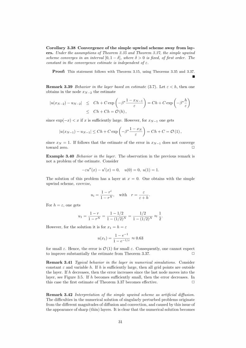
Remark 3.41 Typical behavior in the layer in numerical simulations. Considerconstant ε and variable h. If h is sufficiently large, then all grid points are outsidethe layer. If h decreases, then the error increases since the last node moves into thelayer, see Figure 3.5. If h becomes sufficiently small, then the error decreases. Inthis case the first estimate of Theorem 3.37 becomes effective. 2

Remark 3.42 Interpretation of the simple upwind scheme as artificial diffusion.

The difficulties in the numerical solution of singularly perturbed problems originatefrom the different magnitudes of diffusion and convection, and caused by this issue ofthe appearance of sharp (thin) layers. It is clear that the numerical solution becomes

31

101

102

103

10−3

10−2

10−1

100

number of nodese

rro

r in

th

e d

iscre

te m

axim

um

no

rm

Figure 3.5: Error of the simple upwind scheme for Example 2.8, ε = 1e − 3, anddifferent number of nodes.

the simpler, the larger the diffusion, compared with the convection, become and thelayers become wider.

Consider b > 0, then it is

biDNui = biD

−ui =ui − ui−1

h= bi

ui+1 − ui−1

2h+ bi

−ui+1 + 2ui − ui−1

2h

= biD0ui −

bih

2D+D−ui.

Hence, the simple upwind scheme (3.6) can be written in the form

−

(

ε+bih

2

)

D+D−ui + biD0ui + ciui = fi, for i = 1, . . . , N − 1,

u0 = uN = 0. (3.9)

One can see that the diffusion coefficient is artificially increased and it hasthe magnitude O (h). Consequently, the simple upwind scheme is nothing elsethen a central difference scheme applied to a problem with sufficiently large, O (h),diffusion. It has been observed already in Example 3.30 that the central differencescheme gives useful results if the diffusion is of order O (h).

One can define methods with artificial diffusion also directly. 2

Definition 3.43 Scheme with artificial diffusion, fitted upwind scheme. Afinite difference scheme with artificial diffusion is defined by

− εσ (q(xi))D+D−ui + biD

0ui + ciui = fi, for i = 1, . . . , N − 1,

u0 = uN = 0, (3.10)

q(x) :=b(x)h

2ε,

and σ(q) is an appropriate function. It is also called fitted upwind scheme. 2

Remark 3.44 Fitted upwind schemes.

• The simple upwind scheme (3.6) is obtained for σ(q) = 1 + q, see (3.9).• The introduction of artificial diffusion changes the original problem significantly.Consider, e.g.,

−εu′′ + u′ = 1 in (0, 1), u(0) = u(1) = 0,

with the solution

u(x) = x−exp

(

− 1−xε

)

− exp(

− 1ε

)

1− exp(

− 1ε

) , (3.11)

32

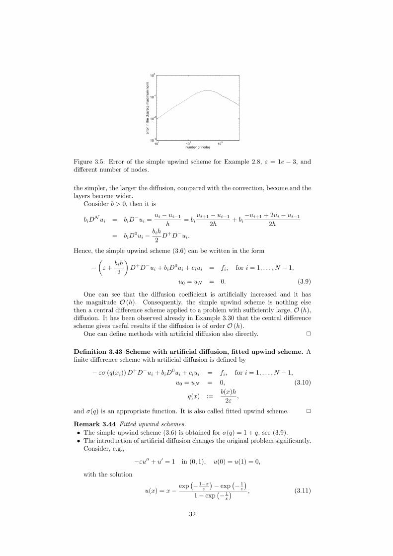
see Example 2.8. The second term is responsible for the satisfaction of theboundary condition at x = 1. It is basically different from zero only in the inter-val [1− ε, 1], see Figure 3.6. Introducing artificial diffusion leads to a perturbedsolution and the term, which is responsible for the satisfaction of the boundarycondition, is in the interval [1−εσ(q(xN−1)), 1] considerably different from zero.That means, the layer is by far less steep. This effect is called smearing of thelayer.

Figure 3.6: Second term of the solution (3.11) for ε = 10−6.

For the simple upwind scheme, it is

εσ(q(xN−1)) = ε+ εbN−1h

2ε= ε+

bN−1h

2.

This expression is in realistic situations, i.e., for ε bN−1 and ε h, larger byorders of magnitude than ε.

2

Remark 3.45 Key point of stabilized methods. Appropriate discretizations forconvection-dominated problems are called stabilized methods. The introductionof artificial diffusion is the key issue of stabilized methods. The difficulty in theconstruction of stabilized methods is that one needs to apply the right amount ofartificial diffusion, at the right locations, and in the correct directions (in multipledimensions).

A question is if one can construct stable methods which lead to less smearing ofthe layers than the simple upwind scheme. 2

Theorem 3.46 Stability of schemes with artificial diffusion. Let b(x) >β > 0, c(x) ≥ 0, and σ(q) > q. Then, the matrix of the scheme with artificial

diffusion (3.10) is an M-matrix and the method is stable in the discrete maximum

norm. The stability constant does not depend on ε.

Proof: The proof is very similar to the proof of Theorem 3.35, exercise.

Theorem 3.47 Consistency of schemes with artificial diffusion. Let the

assumptions of Theorem 3.46 be satisfied, let u ∈ C4([0, 1]), and let

|σ(q)− 1| ≤ minq,Mq2,

with a constant M > 0. Then, for fixed ε, the consistency error of the scheme with

artificial diffusion (3.10) is of second order.

33

Proof: The consistency error in the node xi is

|τi| =∣

∣

[

− εσ (qi)D+D−u(xi) + biD

0u(xi) + ciu(xi)]

−[

− εu′′(xi) + biu′(xi) + ciu(xi)

]∣

∣

=∣

∣εσ(qi)(

u′′(xi)−D+D−ui

)

+ ε (1− σ(qi))u′′(xi) + bi

(

D0u(xi)− u′(xi))∣

∣ .

From the consistency error estimate in Example 3.7 it follows that

|τi| ≤ C(

εσ(qi)h2∥

∥

∥u(4)

∥

∥

∥

∞

+ ε |1− σ(qi)|∥

∥u′′∥

∥

∞+ h2

∥

∥

∥u(3)

∥

∥

∥

∞

)

.

Using the assumptions of the theorem and the definition of q(x) gives

σ(qi) ≤ |σ(qi)− 1|+ 1 ≤ min

qi,Mq2i

+ 1 ≤ qi + 1 ≤ Ch

ε+ 1,

|1− σ(qi)| ≤ Mq2i ≤ Ch2

ε2.

Inserting this estimate yields

|τi| ≤ C

((

h

ε+ 1

)

εh2∥

∥

∥u(4)

∥

∥

∥

∞

+ εh2

ε2∥

∥u′′∥

∥

∞+ h2

∥

∥

∥u(3)

∥

∥

∥

∞

)

(3.12)

≤ C(ε)h2.

Remark 3.48 The consistency of the scheme with artificial diffusion.

• Examples of functions σ(q) that satisfy the assumptions of Theorem 3.47 are(exercise)

σ(q) = max1, q, σ(q) =√

1 + q2, σ(q) = 1 +q2

1 + q.

The last variant is called Samarskii upwind scheme.• The consistency is of second order only for constant ε. The factor C(ε) divergesto infinity for ε → 0, see the middle term in (3.12). In addition, also derivativesof the solution might depend in a bad way on ε and they might explode forε → 0. It follows that these methods become worse and worse for ε → 0. Onecan show that the consistency independent of ε away from the layer is only offirst order. The typical behavior in the layer is analogously as for the simpleupwind scheme, see Remark 3.41.

2

Remark 3.49 Summary.

• The central difference scheme is not suited for singularly perturbed problems.• The simple upwind scheme is stable, but too inaccurate (of first order consistent).

Layers are heavily smeared.• Upwind methods can be interpreted as methods with artificial diffusion.• Fitted upwind methods might be of second order consistent, but only for fixedε. This property is not uniform in ε.

The upwind schemes that have been introduced so far are not satisfactory sincethey are too inaccurate for small ε and the convergence in the layer depends on ε.

2

34

Figure 3.7: Alexander Andreewitsch Samarskii (1919 – 2008).

3.4 Uniformly Convergent Methods

Remark 3.50 Motivation. The goal consists in the development of discretizationswhich converge uniformly in the whole interval [0, 1], in particular in the layer. Twoways for achieving this goal will be presented:

• a scheme which is obtained with an appropriate choice of artificial diffusion σ(q)in (3.10),

• schemes, which are defined by an appropriate choice of the grid.

In practice, one often has very small diffusion. Therefore it is important to constructnumerical methods which provide accurate results in this case. The constructionof such methods is not trivial. This might become clear already from the fact thatthe limit ε → 0 is in a certain sense discontinuous, since the order of the differentialequation changes. With this change of order, also other important features change,e.g., the needed boundary conditions to define a well-posed problem. Also theproperties of the solutions of differential equations with different order are different,e.g., the smoothness properties. A uniformly convergent method has to deal withthis limit without deterioration of the quality of the computed solution.

This section follows in part Großmann and Roos (2005). 2

Definition 3.51 Uniform convergence. A scheme for the solution of (3.4), (3.5)is called uniformly convergent of order p with respect to the singularly perturbationparameter ε in the discrete maximum norm if an estimate of the form

‖u− uh‖∞,d ≤ Chp, p > 0,

holds with a constant C that does not depend on ε. 2

3.4.1 Sophisticated Artificial Diffusion

Remark 3.52 Idea. The choice of a sophisticated artificial diffusion σ(q) can bemotivated with a study of the solution of (3.4), (3.5) for ε → 0. 2

Lemma 3.53 Convergence to the reduced solution. Let u(x, ε) be the solu-

tion of (3.4), (3.5) with b(x) ≥ β > 0, c(x) ≥ 0, and let u0(x) be the solution of the

reduced problem. Then it holds for all x ∈ [0, x0) with x0 < 1 that

limε→0

u(x, ε) = u0(x).

35

Proof: The proof is based on the comparison principle, Corollary 2.34. Set

v1(x) := γ exp(βx), γ > 0,

then it follows that

(Lv1)(x) = γ(−εβ2 + b(x)β + c(x)) exp(βx) ≥ γβ2(1− ε) exp(βx) ≥ 1

for sufficiently large γ. Now, let

v2(x) := exp

(

−β1− x

ε

)

,

then it holds

(Lv2)(x) =

(

−εβ2

ε2+ b(x)

β

ε+ c(x)

)

exp

(

−β1− x

ε

)

≥β

ε(−β + b(x)) exp

(

−β1− x

ε

)

≥ 0.

Consider nowv(x) := M1εv1(x) +M2v2(x),

then one obtains, for appropriately chosen constants M1 and M2 and using the estimatesfor (Lv1)(x) and (Lv2)(x),

(Lv)(x) = M1ε(Lv1)(x) +M2(Lv2)(x) ≥ M1ε(Lv1)(x) ≥ M1ε ≥ ε∣

∣u′′

0 (x)∣

∣

= |L(u− u0)(x)| ,

v(0) = M1εv1(0) +M2v2(0) = M1εγ +M2 exp(−β/ε) ≥ 0 = |(u− u0)(0)| ,

v(1) = M1εv1(1) +M2v2(1) = M1εγ exp(β) +M2 ≥ M2 ≥ |(u− u0)(1)| = |u0(1)| .

The constants have to be sufficiently large and they only depend on u0(x). There is nocoefficient ε in the reduced problem such that u0(x) cannot depend on ε and hence theconstants do not depend on ε. With the comparison principle it follows that

|(u− u0)(x)| ≤ v(x) = M1εγ exp(βx) +M2 exp

(

−β1− x

ε

)

.

Hence, one gets for x < 1limε→0

|(u− u0)(x)| = 0.

Lemma 3.54 Estimate to the reduced solution plus a correction term.

Under the assumptions of Lemma 3.53, there is a constant C, which is independent

of x and ε, such that for the solution of (3.4), (3.5) it holds∣

∣

∣

∣

u(x, ε)−

[

u0(x)− u0(1) exp

(

−b(1)1− x

ε

)]∣

∣

∣

∣

≤ Cε, x ∈ [0, 1].

Proof: The proof is similar to the proof of Lemma 3.53.

Remark 3.55 Necessary condition for a sophisticated artificial diffusion σ(q). Letρ∗ := h/ε be fixed, i.e., for h → 0 it holds also ε → 0. The goal consists in finding forthis case a condition for an appropriate function σ(q) in the fitted upwind scheme.

Let a node i be fixed. Since ε → 0 for h → 0 it follows from Lemma 3.54 that

limh→0

u(1− ih) = limh→0

(

u0(1− ih)− u0(1) exp

(

−b(1)1− (1− ih)

ε

))

= u0(1)− u0(1) limh→0

exp

(

−b(1)ih

ε

)

= u0(1)− u0(1) exp (−ib(1)ρ∗)

= u0(1) (1− exp(−2iq(1)) , (3.13)

36

where the definition of q(x) has been used. The fitted upwind scheme has the form

−εσ (q(bi))ui+1 − 2ui + ui−1

h2+ bi

ui+1 − ui−1

2h= fi − ciui,

or after multiplication with h2/ε

−σ (q(bi)) (ui+1 − 2ui + ui−1) + q(bi) (ui+1 − ui−1) =h2

ε(fi − ciui)

= hρ∗ (fi − ciui) .

For the right boundary, i.e., i = N − 1, it is in particular

limh→0

(−σ (qN−1) (uN − 2uN−1 + uN−2) + qN−1 (uN − uN−2))

= limh→0

hρ∗ (fN−1 − cN−1uN−1) = 0,

since f(x), c(x) are bounded and ρ∗ is a constant. Inserting of (3.13) gives, whereon has to take in (3.13) the indices i ∈ 0, 1, 2 and one assumes without loss ofgenerality u0(1) 6= 0,

0 = −σ (q(1))(

− exp(0) + 2 exp(−2q(1))− exp(−4q(1)))

+q(1)(

− exp(0) + exp(−4q(1)))

.

It is, using the binomial theorem,

−1 + e−4x

−1 + 2e−2x − e−4x=

(e−2x − 1)(e−2x + 1)

−(e−2x − 1)2=

1 + e−2x

1− e−2x=

ex + e−x

ex − e−x= coth(x).

Hence, one gets as necessary condition

σ (q(1)) = q(1)1− exp(−4q(1))

1− 2 exp(−2q(1)) + exp(−4q(1))= q(1) coth (q(1)) .

One choice which satisfies this limit is

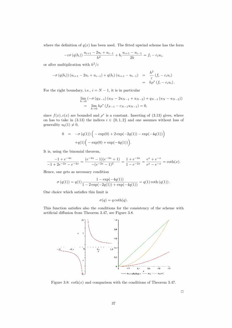
σ(q) = q coth(q).

This function satisfies also the conditions for the consistency of the scheme withartificial diffusion from Theorem 3.47, see Figure 3.8.

Figure 3.8: coth(x) and comparison with the conditions of Theorem 3.47.

2

37

Definition 3.56 Iljin scheme, Iljin–Allen–Southwell scheme. The scheme

−h

2bi coth

(

h

2εbi

)

D+D−ui + biD0ui + ciui = fi, for i = 1, . . . , N − 1,

u0 = uN = 0,

is called Iljin scheme or Iljin–Allen–Southwell (Il’in (1969); Allen and Southwell(1955)) scheme. In some applications it is called also Scharfetter–Gummel scheme(Scharfetter and Gummel (1969)). 2

Theorem 3.57 Uniform convergence of the Iljin–Allen–Southwell scheme.

The Iljin–Allen–Southwell scheme converges in [0, 1] uniformly of first order in the

discrete maximum norm, i.e., it holds

maxi=1,...,N−1

|u(xi)− ui| ≤ Ch

with a constant C that is independent of ε and h.

Proof: The proof is rather long and involved, e.g., see Roos et al. (2008).

Example 3.58 Iljin–Allen–Southwell scheme. Consider

−εu′′ + u′ = 1 in (0, 1), u(0) = u(1) = 0,

with the solution

u(x) = x−exp

(

− 1−xε

)

− exp(

− 1ε

)

1− exp(

− 1ε

) .

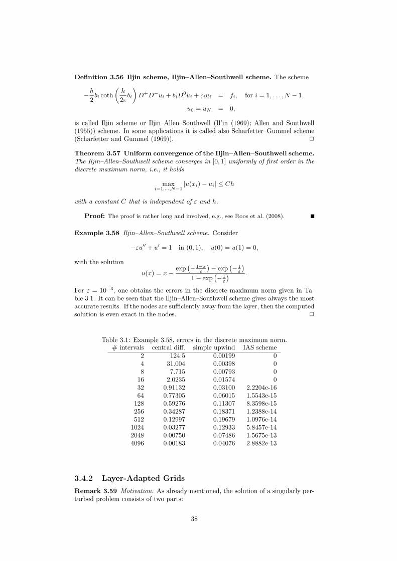
For ε = 10−3, one obtains the errors in the discrete maximum norm given in Ta-ble 3.1. It can be seen that the Iljin–Allen–Southwell scheme gives always the mostaccurate results. If the nodes are sufficiently away from the layer, then the computedsolution is even exact in the nodes. 2

Table 3.1: Example 3.58, errors in the discrete maximum norm.# intervals central diff. simple upwind IAS scheme

2 124.5 0.00199 04 31.004 0.00398 08 7.715 0.00793 016 2.0235 0.01574 032 0.91132 0.03100 2.2204e-1664 0.77305 0.06015 1.5543e-15128 0.59276 0.11307 8.3598e-15256 0.34287 0.18371 1.2388e-14512 0.12997 0.19679 1.0976e-14

1024 0.03277 0.12933 5.8457e-142048 0.00750 0.07486 1.5675e-134096 0.00183 0.04076 2.8882e-13

3.4.2 Layer-Adapted Grids

Remark 3.59 Motivation. As already mentioned, the solution of a singularly per-turbed problem consists of two parts:

38

• the solution of the reduced problem, which is generally smooth and easily toapproximate numerically,

• the correction term, which enforces the boundary condition at the outflowboundary. This term is responsible for the appearance of the layer, i.e., forthe dramatic change of the solution in a very small interval.

Consider as typical example the two-point boundary value problem from Exam-ple 3.58. In the interval [0, 1 − ε], the solution has practically the form u(x) = x.This solution can be easily approximated on a coarse grid. The interesting part ofthe solution is in the interval [1− ε, 1]. If one chooses an equidistant grid with themesh width h, then it is generally h ε. Hence, the interval [1− ε, 1] is containedin [xN−1, xN ] = [1 − h, 1]. Consequently, one cannot expect with this choice toresolve the solution in [1− ε, 1] in a good way.

The idea of layer-adapted grids is to choose in the layer region a considerablyfiner grid than outside the layer region. This approach offers the possibility toapproximate the solution in the layer well. 2

Remark 3.60 Shishkin1 mesh. Consider, for simplicity of notation, a problemwhere the layer is situated at x = 0. In addition, let b = −β, β ∈ R

+, a constant.The grid points are distributed in the form

xi = φ(i/N),

where one has to choose the function φ(ξ) in such a way that one obtains in aneighborhood of x = 0 a sufficiently fine mesh. The number N of intervals is given.

A mesh of Shishkin type is defined by

φ(ξ) =

σε

βφ(ξ) for ξ ∈ [0, 1/2],

1− 2

(

1−σε

βln(N)

)

(1− ξ) for ξ ∈ [1/2, 1],

with φ(1/2) = ln(N) and the parameter σ > 0. The Shishkin mesh (1988) isobtained with

φ(ξ) = 2 ln(N)ξ.

With this choice, one has for the nodes x0, . . . , xN/2, i ≥ 1,

xi − xi−1 = φ

(

i

N

)

− φ

(

i− 1

N

)

=σε

β2 ln(N)

(

i

N−

i− 1

N

)

= 2σε

β

ln(N)

N,

independent of i. For the nodes xN/2+1, . . . , xN , it is for i ≥ N/2 + 1,

xi − xi−1 = φ

(

i

N

)

− φ

(

i− 1

N

)

= 1− 2

(

1−σε

βln(N)

)(

1−i

N

)

− 1 + 2

(

1−σε

βln(N)

)(

1−i− 1

N

)

=2

N− 2

σε

β

ln(N)

N,

independent of i. Hence, a piecewise equidistant mesh is defined. The transitionpoint from the very fine to the coarse grid is located at

τ = xN/2 =σε

βln(N).

The use of the Shishkin mesh is supported by results from the numerical analysis.2

1Grigory I. Shishkin

39

Theorem 3.61 Convergence of the simple upwind scheme on a Shishkin

mesh. Consider the simple upwind scheme on a Shishkin mesh with the transition

point

τ = min

1

2,ε

βln(N)

,

i.e., with σ = 1. Then it holds the following error estimate

maxi=1,...,N−1

|u(xi)− ui| ≤ CN−1 ln(N),

where the constant C is independent of ε and N .

Proof: The proof is based on the decomposition of the solution in the part coming

from the reduced problem (smooth part) and the correction part. It is rather long and

involved, see Roos et al. (2008).

Remark 3.62 Layer-adapted meshes.

• The convergence is slightly suboptimal because of the factor ln(N). However,one can see in numerical examples that the given error estimate is sharp, i.e.,this factor cannot be omitted.

• The idea to used layer-adapted mesh goes back to Bahvalov2 (Bahvalov (1969)).In Bahvalov meshes, there is a smooth transition from the fine to the coarsemesh. However, the numerical analysis for schemes on Bahvalov meshes is ingeneral more complicated than on Shishkin meshes.

• The a priori (before the numerical simulation) construction of appropriate layer-adapted meshes needs more or less already the knowledge of the solution. Thisaspect is in applications not given, in particular for problems in two or threedimensions. Then, one needs an a posteriori (during the numerical simulation)construction of adapted grids. There are ways to perform this approach.

• An essential finding of the analysis of numerical methods on a priori layer-adapted grids is that one can use on an appropriate grids a simple numericalmethod and one obtains reasonable error estimates.

• Using a Shishkin mesh, one has to define the finite differences in the node xN/2,where the distances to the neighbor nodes are of different lengths.Let xi be a node and let the intervals [xi−1, xi] and [xi, xi+1] have the lengthhi and hi+1, respectively. There are no changes for the backward and forwardfinite difference compared with Definition 3.4, since for them one needs only oneof the neighbor intervals. Define

hi :=hi + hi+1

2,

then the central difference is the weighted average

D0v(xi) =1

2hi

(

hiD+v(xi) + hi+1D

−v(xi))

.

The second derivative is approximated by

v′′(xi) ≈1

hi

(

D+v(xi)−D−v(xi))

=1

hi

(

vi+1 − vihi+1

−vi − vi−1

hi

)

.

• The matrices, which are obtained when using layer-adapted meshes, have gen-erally a very bad condition number.

2Nikolai Sergejewitsch Bahvalov (1934 – 2005)

40

• Layer adapted meshes can be applied in the finite element context in the samefashion as for finite difference methods.

• A comprehensive monograph about numerical methods on layer-adapted meshesis Linß (2010).

2

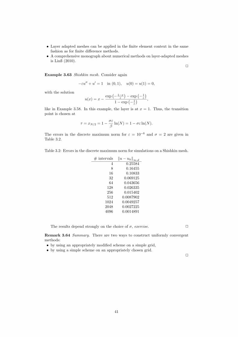
Example 3.63 Shishkin mesh. Consider again

−εu′′ + u′ = 1 in (0, 1), u(0) = u(1) = 0,

with the solution

u(x) = x−exp

(

− 1−xε

)

− exp(

− 1ε

)

1− exp(

− 1ε

) ,

like in Example 3.58. In this example, the layer is at x = 1. Thus, the transitionpoint is chosen at

τ = xN/2 = 1−σε

βln(N) = 1− σε ln(N).

The errors in the discrete maximum norm for ε = 10−6 and σ = 2 are given inTable 3.2.

Table 3.2: Errors in the discrete maximum norm for simulations on a Shishkin mesh.

# intervals ‖u− uh‖∞,d

4 0.255848 0.1645516 0.1083332 0.06912564 0.043656128 0.026335256 0.015402512 0.0087902

1024 0.00492572048 0.00272254096 0.0014891

The results depend strongly on the choice of σ, exercise. 2

Remark 3.64 Summary. There are two ways to construct uniformly convergentmethods:

• by using an appropriately modified scheme on a simple grid,• by using a simple scheme on an appropriately chosen grid.

2

41