Embed Size (px)
Citation preview

Finite difference methods for the time fractionalorder differential equations
Zhi-zhong SunDepartment of Mathematics, Southeast University,
Nanjing 210096, P R China(e-mail: [email protected],)
Joint work withWanrong Cao, Rui Du, Guanghua Gao, Jincheng Ren
Xiaonan Wu, Yanan Zhang, Xuan Zhao
Fractional PDEs Confernce
June 3-5, 2013
In this talk, I’d like to present an overview of our recent works onthe finite difference methods for the time fractional differentialequation.

Outline
Approximations to the Caputo’s fractional derivatives
Finite difference methods for the time fractional sub-diffusionequation
Dirichlet boundary conditionsNeumann boundary conditionSpace unbounded domain problem
Finite difference methods for the time fractional diffusion-waveequation
Dirichlet boundary conditionsNeumann boundary conditions
Finite difference methods for the multi-term time fractionaldiffusion-wave equation
ADI methods for the multi-dimensional time fractional equationsFractional sub-diffusion equationFractional diffusion-wave equation

1.1 Definition of the Caputo fractional derivative
For a given positive real number γ, n − 1 < γ 6 n, the Caputofractional derivative with the order of γ, is defined by
C0 D
γt f (t) =
1
Γ(n − γ)
∫ t
0
f (n)(ξ)
(t − ξ)γ−n+1dξ.
I Case γ ∈ (0, 1) :
C0 D
γt f (t) =
1
Γ(1− γ)
∫ t
0
f ′(ξ)
(t − ξ)γdξ.
I Case γ ∈ (1, 2) :
C0 D
γt f (t) =
1
Γ(2− γ)
∫ t
0
f ′′(ξ)
(t − ξ)γ−1dξ.

1.2 Approximation of the fractional derivative: γ = 12
Theorem [Sun and Wu 2004 ANM]
Suppose f (t) ∈ C 2[0, tn] Let
R(f (tn)) ≡ C0 D
12t f (tn)−
τ−12
Γ(2− 12)
[a0f (tn)−
n−1∑k=1
(an−k−1 − an−k
)f (tk)− an−1f (t0)
],
then
|R(f (tn))| 61
6√π
(10√
2− 11)
max06t6tn
|f ′′(t)|τ32 ,
where al =√
l + 1−√
l , l > 0.

1.3 Approximation of the fractional derivative: γ ∈ (0, 1)
Theorem [Sun and Wu 2006 ANM]
Suppose f (t) ∈ C 2[0, tn] and γ ∈ (0, 1). Let
R(f (tn)) ≡ C0 D
γt f (tn)−
τ−γ
Γ(2− γ)
[a0f (tn)−
n−1∑k=1
(an−k−1 − an−k
)f (tk)− an−1f (t0)
],
then
|R(f (tn))| 61
Γ(2− γ)
[1− γ
12+
22−γ
2− γ−(1+2−γ)
]max
06t6tn|f ′′(t)|τ2−γ ,
where al = (l + 1)1−γ − l1−γ , l > 0.

1.4 Approximation of the fractional derivative: γ ∈ (1, 2)
Theorem [Sun and Wu 2006 ANM]
Suppose f (t) ∈ C 3[0, tn] and γ ∈ (1, 2). Let
R(f (tn)) ≡1
2
[C0 D
γt f (tn) + C
0 Dγt f (tn−1)
]−
τ1−γ
Γ(3− γ)
[b0δt f
n− 12 −
n−1∑k=1
(bn−k−1 − bn−k
)δt f
k− 12 − 1
2bn−1f
′(t0)],
then
|R(f (tn))| 61
Γ(3− γ)
(2− γ
12+
23−γ
3− γ− 21−γ − 5
6
)max
06t6tn|f ′′′(t)|τ3−γ ,
where
bl = (l+1)2−γ−l2−γ , l > 0, δt fk− 1
2 =f (tk)− f (tk−1)
τ, 1 6 k 6 n.

2.1 Dirichlet boundary problem of the sub-diffusionequation
Consider the following one-dimensional problem
C0 Dα
t u(x , t) = κα∂2u(x , t)
∂x2+ f (x , t), a < x < b, 0 < t 6 T ,
(1)
u(x , 0) = ψ(x), a 6 x 6 b, (2)
u(a, t) = ϕ1(t), u(b, t) = ϕ2(t), 0 < t 6 T , (3)
where α ∈ (0, 1).
The fractional equation (1) is called the time fractionalsub-diffusion equation.

2.1 Dirichlet boundary problem of the sub-diffusionequation
For finite difference approximation, discretize equally the interval[a, b] with xi = a + ih (0 6 i 6 M), [0,T ] withtk = kτ (0 6 k 6 N), where h = 1/M and τ = T/N are thespatial and temporal step sizes, respectively. First the followingnotations are introduced.
δxui− 12
=1
h(ui − ui−1), δ2xui =
1
h
(δxui+ 1
2− δxui− 1
2
),
‖u‖∞ = max0≤i≤M
|ui |, Aui =1
12(ui−1 + 10ui + ui+1), 1 6 i 6 M − 1,
In addition, denote a discrete fractional derivative operator Dατ
Dατ uk
i =1
µ
[uki −
k−1∑j=1
(ak−j−1−ak−j)uji−ak−1u
0i
], 0 6 i 6 M, 1 6 k 6 N.
Define the grid function
Uki = u(xi , tk), 0 6 i 6 M, 0 6 k 6 N.

2.1 Dirichlet boundary problem of the sub-diffusionequation
In 2006, we constructed the following difference scheme
Dατ uk
i = καδ2xu
ki + f k
i , 1 6 i 6 M − 1, 1 6 k 6 N, (4)
u0i = ψ(xi ), 0 6 i 6 M, (5)
uk0 = ϕ1(tk), uk
M = ϕ2(tk), 1 6 k 6 N. (6)
We proved that

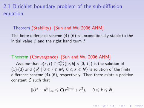
2.1 Dirichlet boundary problem of the sub-diffusionequation
Theorem (Stability) [Sun and Wu 2006 ANM]
The finite difference scheme (4)-(6) is unconditionally stable to theinitial value ψ and the right hand term f .
Theorem (Convergence) [Sun and Wu 2006 ANM]
Assume that u(x , t) ∈ C4,2x ,t ([a, b]× [0,T ]) is the solution of
(1)-(3) and uki | 0 6 i 6 M, 0 6 k 6 N is solution of the finite
difference scheme (4)-(6), respectively. Then there exists a positiveconstant C such that
‖Uk − uk‖∞ 6 C (τ2−α + h2), 0 6 k 6 N.

2.1 Dirichlet boundary problem of the sub-diffusionequation
In 2011, we established the following difference scheme
ADατ uk
i = καδ2xu
ki +Af k
i , 1 6 i 6 M − 1, 1 6 k 6 N, (7)
u0i = ψ(xi ), 0 6 i 6 M, (8)
uk0 = ϕ1(tk), uk
M = ϕ2(tk), 1 6 k 6 N. (9)
We proved that
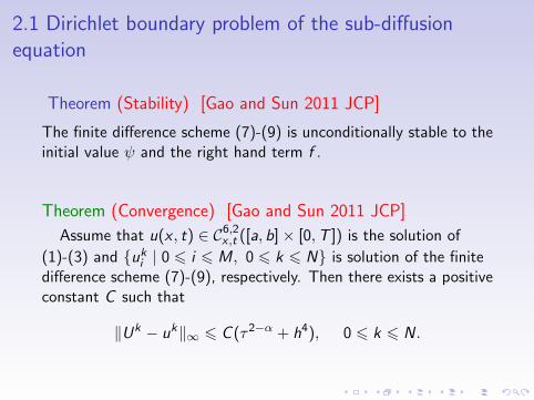
2.1 Dirichlet boundary problem of the sub-diffusionequation
Theorem (Stability) [Gao and Sun 2011 JCP]
The finite difference scheme (7)-(9) is unconditionally stable to theinitial value ψ and the right hand term f .
Theorem (Convergence) [Gao and Sun 2011 JCP]
Assume that u(x , t) ∈ C6,2x ,t ([a, b]× [0,T ]) is the solution of
(1)-(3) and uki | 0 6 i 6 M, 0 6 k 6 N is solution of the finite
difference scheme (7)-(9), respectively. Then there exists a positiveconstant C such that
‖Uk − uk‖∞ 6 C (τ2−α + h4), 0 6 k 6 N.

2.1 Dirichlet boundary problem of the sub-diffusionequation
In (1)-(3), let a = 0, b = 1, T = 1, κγ = 1,
f (x , t) = ex[(1 + γ)tγ − Γ(2 + γ)
Γ(1 + 2γ)t2γ
],
ϕ1(t) = t1+γ , ϕ2(t) = et1+γ , u(x , 0) = 0.
Then the exact solution is
u(x , t) = ex t1+γ .
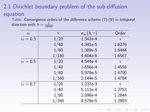
2.1 Dirichlet boundary problem of the sub-diffusionequation
Table: Convergence orders of the difference scheme (7)-(9) in temporaldirection with h = 1
20000 .
α τ e∞(h, τ) Order
α = 0.3 1/20 1.341e-4 ∗1/40 4.341e-5 1.62761/80 1.389e-5 1.64441/160 4.404e-6 1.6567
α = 0.5 1/20 4.544e-4 ∗1/40 1.656e-4 1.45581/80 5.979e-5 1.47001/160 2.144e-5 1.4794
α = 0.7 1/20 1.237e-3 ∗1/40 5.111e-4 1.27531/80 2.098e-4 1.28441/160 8.579e-5 1.2903
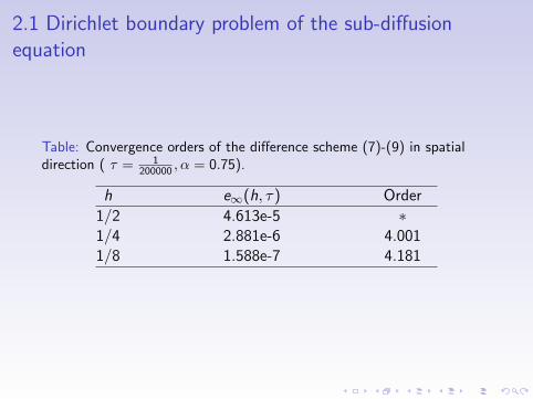
2.1 Dirichlet boundary problem of the sub-diffusionequation
Table: Convergence orders of the difference scheme (7)-(9) in spatialdirection ( τ = 1
200000 , α = 0.75).
h e∞(h, τ) Order
1/2 4.613e-5 ∗1/4 2.881e-6 4.0011/8 1.588e-7 4.181

2.2 Neumann boundary problem of the sub-diffusionequation
Consider the following one-dimensional time fractionalsub-diffusion equation
C0 Dα
t u(x , t) =∂2u(x , t)
∂x2+ f (x , t), a < x < b, 0 < t 6 T , (10)
u(x , 0) = ϕ(x), a 6 x 6 b, (11)
∂u(a, t)
∂x= 0,
∂u(b, t)
∂x= 0, 0 < t 6 T . (12)
where α ∈ (0, 1).

2.2 Neumann boundary problem of the sub-diffusionequation
In 2011, We constructed the following spatial second orderdifference scheme
Dατ uk
12
=2
hδxu
k12
+ f k12, 1 6 k 6 N, (13)
1
2(Dα
τ uki− 1
2+ Dα
τ uki+ 1
2) = δ2xu
ki +
1
2(f k
i− 12
+ f ki+ 1
2),
1 6 i 6 M − 1, 1 6 k 6 N, (14)
Dατ uk
M− 12
= −2
hδxu
kM− 1
2+ f k
M− 12, 1 6 k 6 N, (15)
u0i = ψ(xi ), 0 6 i 6 M. (16)
We proved that

2.2 Neumann boundary problem of the sub-diffusionequation
Theorem (Stability) [Zhao and Sun 2011 JCP, Ren]
The finite difference scheme (13)-(16) and (17)-(20) isunconditionally stable to the initial value ψ and the right handterm f .
Theorem (Convergence) [Zhao and Sun 2011 JCP]
Assume that u(x , t) ∈ C4,2x ,t ([a, b]× [0,T ]) is the solution of
(10)-(12) and uki | 0 6 i 6 M, 0 6 k 6 N is solution of the
finite difference scheme (13)-(16), respectively. Then there exists apositive constant C such that
‖Uk − uk‖∞ 6 C (τ2−α + h2), 0 6 k 6 N.

2.2 Neumann boundary problem of the sub-diffusionequation
In 2013, we presented the following spatial fourth order finitedifference scheme
BDατ uk
0 =2
hδxu
k12
+h
6(fx)
k0 + Bf k
0 , 1 6 k 6 N, (17)
BDατ uk
i = δ2xuki + Bf k
i , 1 6 i 6 M − 1, 1 6 k 6 N, (18)
BDατ uk
M = −2
hδxu
kM− 1
2− h
6(fx)
kM + Bf k
M , 1 6 k 6 N, (19)
u0i = ψ(xi ), 0 6 i 6 M, (20)
where
Bui =
1
6(5u0 + u1), i = 0,
1
12(ui−1 + 10ui + ui+1), 1 6 i 6 M − 1,
1
6(uM−1 + 5uM), i = M.

2.2 Neumann boundary problem of the sub-diffusionequation
Theorem (Stability) [Sun and Zhao, 2013 JCP]
The finite difference schemes (17)-(20) is unconditionally stable tothe initial value ψ and the right hand term f .
Theorem (Convergence) [Ren, Sun and Zhao 2013 JCP]
Assume that u(x , t) ∈ C6,2x ,t ([a, b]× [0,T ]) is the solution of
(10)-(12) and uki | 0 6 i 6 M, 0 6 k 6 N is solution of the
finite difference scheme (17)-(20), respectively. Then there exists apositive constant C such that
‖Uk − uk‖ 6 C (τ2−α + h4), 0 6 k 6 N.

2.2 Neumann boundary problem of the sub-diffusionequation
In (10), let T = 1. In order to test the convergence rate of theproposed methods, we consider the exact solution of the problem(10)-(12) as follows
u(x , t) = exx2(1− x)2tγ+2.
Then it can be checked that the corresponding forcing term f (x , t)and initial condition ϕ(x) are respectively
f (x , t) =Γ(γ + 3)
2t2exx2(1−x)2−ex tγ+2(2−8x +x2 +6x3 +x4),
andϕ(x) = 0.

2.2 Neumann boundary problem of the sub-diffusionequation
Table: Convergence orders of both schemes in temporal direction withh = 1
20000 .
α τ e∞(h, τ) Order
α = 0.3 1/20 1.341e-4 ∗1/40 4.337e-5 1.64691/80 1.385e-5 1.66471/160 4.368e-6 1.6915
α = 0.5 1/20 4.543e-4 ∗1/40 1.656e-4 1.47041/80 5.977e-5 1.48061/160 2.142e-5 1.4892
α = 0.7 1/20 1.237e-3 ∗1/40 5.111e-4 1.28451/80 2.098e-4 1.29051/160 8.577e-5 1.2946
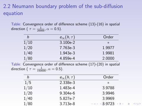
2.2 Neumann boundary problem of the sub-diffusionequation
Table: Convergence order of difference scheme (13)-(16) in spatialdirection ( τ = 1
20000 , α = 0.5).
h e∞(h, τ) Order
1/10 3.100e-2 ∗1/20 7.763e-3 1.99771/40 1.943e-3 1.99811/80 4.859e-4 2.0000
Table: Convergence order of difference scheme (17)-(20) in spatialdirection ( τ = 1
150000 , α = 0.5).
h e∞(h, τ) Order
1/5 2.338e-3 ∗1/10 1.483e-4 3.97881/20 9.304e-6 3.99461/40 5.827e-7 3.99691/80 3.713e-8 3.9723

2.2 Neumann boundary problem of the sub-diffusionequation
Table: The maximum norm error and CPU time of two schemes.
scheme (17)-(20) scheme (13)-(16)α N M e∞(h, τ) CPU time(s) M e∞(h, τ) CPU time(s)
0.3 585 15 3.335e-5 0.4907 225 7.645e-5 6.66281151 20 1.056e-5 1.4478 400 2.419e-5 26.98301947 25 4.330e-6 3.6058 625 9.906e-6 85.89402989 30 2.089e-6 7.9330 900 4.777e-6 232.3370
0.5 1368 15 3.022e-5 1.3981 225 6.057e-5 19.11512947 20 9.571e-6 5.3454 400 1.916e-5 101.84545344 25 3.922e-6 16.7761 625 7.850e-6 406.50718689 30 1.892e-6 44.7167 900 3.785e-6 1344.5115
0.7 4157 15 2.747e-5 6.8338 225 4.692e-5 98.229110073 20 8.701e-6 40.6099 400 1.484e-5 794.837520015 25 3.566e-6 172.7832 625 6.080e-6 4294.011835074 30 1.720e-6 589.2156 900 2.932e-6 18178.9099

2.3 Space unbounded domain problem for the timefractional sub-diffusion equation
We are concerned with the fractional sub-diffusion equations onthe whole-space
C0 D
γt u(x , t)− Kγuxx(x , t) = f (x , t), (x , t) ∈ Ω = R× [0,T ],
(21)
u(x , 0) = ψ(x), x ∈ R, (22)
u(x , t) → 0, when x → ±∞, t ∈ (0,T ], (23)
where suppf (x , t) ⊆ [XL,XR ]× [0,T ], suppψ(x) ⊆ [XL,XR ].
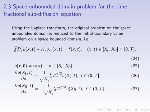
2.3 Space unbounded domain problem for the timefractional sub-diffusion equation
Using the Laplace transform, the original problem on the spaceunbounded domain is reduced to the initial-boundary valueproblem on a space bounded domain, i.e.,
C0 D
γt u(x , t)− Kγuxx(x , t) = f (x , t), (x , t) ∈ [XL,XR ]× (0,T ],
(24)
u(x , 0) = ψ(x), x ∈ [XL,XR ], (25)
∂u(XL, t)
∂x=
1√Kγ
C0 D
γ/2t u(XL, t), t ∈ (0,T ], (26)
∂u(XR , t)
∂x= − 1√
Kγ
C0 D
γ/2t u(XR , t), t ∈ (0,T ]. (27)

2.3 Space unbounded domain problem for the timefractional sub-diffusion equation
We constructed the following spatial second order differencescheme
Dγτ uk
i − Kγδ2xu
ki = f k
i , 1 ≤ i ≤ M − 1, 1 ≤ k ≤ N, (28)
Dγτ uk
0 −2Kγ
h
[δxu
k12− 1√
Kγ
Dγ/2τ uk
0
]= f k
0 , 1 ≤ k ≤ N, (29)
Dγτ uk
M − 2Kγ
h
[− 1√
Kγ
Dγ/2τ uk
M − δxukM− 1
2
]= f k
M , 1 ≤ k ≤ N,
(30)
u0i = ψ(xi ), 0 ≤ i ≤ M, (31)
and the following spatial fourth order finite difference scheme forthe case of γ ≤ 2/3,

2.3 Space unbounded domain problem for the timefractional sub-diffusion equation
BDγτ uk
0 −2Kγ
h
(δxu
k12− 1√
Kγ
Dγ/2τ uk
0
)= −h
6
1
Kγ
[ 1√Kγ
D3γ/2t uk
0 − fx(x0, tk)]
+ Bf k0 , 1 6 k 6 N, (32)
BDατ uk
i − Kγδ2xu
ki = Bf k
i , 1 6 i 6 M − 1, 1 6 k 6 N, (33)
BDγτ uk
M − 2Kγ
h
(− 1√
Kγ
Dγ/2τ uk
M − δxukM− 1
2
)=
h
6
1
Kγ
[− 1√
Kγ
D3γ/2t uk
M − fx(xM , tk)]
+ Bf kM , 1 6 k 6 N,
(34)
u0i = ψ(xi ), 0 6 i 6 M, (35)

2.3 Space unbounded domain problem for the timefractional sub-diffusion equation
where
D3γ/2t Uk
i =
D
3γ/2t Uk
i , γ < 2/3,
(Uki − Uk−1
i )/τ, γ = 2/3,i = 0, M.
We proved that

2.3 Space unbounded domain problem for the timefractional sub-diffusion equation
Theorem (Stability) [Gao, Sun and Zhang 2013 JCP]
The finite difference schemes (28)-(31) and (32)-(35) areunconditionally stable to the initial value ψ and the right handterm f .
Theorem (Convergence) [Gao, Sun and Zhang 2013 JCP]
Assume that u(x , t) ∈ C4,2x ,t ([a, b]× [0,T ]) is the solution of
(24)-(27) and uki | 0 6 i 6 M, 0 6 k 6 N is solution of the
finite difference scheme (28)-(31), respectively. Then there exists apositive constant C such that√√√√τ
n∑k=1
‖Uk − uk‖2∞ 6 C (τ2−γ + h2), 0 6 n 6 N.

2.3 Space unbounded domain problem for the timefractional sub-diffusion equation
Theorem (Convergence) [Gao, Sun and Zhang 2013 JCP]
Assume that u(x , t) ∈ C6,2x ,t ([a, b]× [0,T ]) is the solution of
(24)-(27) and uki | 0 6 i 6 M, 0 6 k 6 N is solution of the
finite difference scheme (32)-(35), respectively. Then there exists apositive constant C such that√√√√τ
n∑k=1
‖Uk − uk‖2∞ 6 C (τ2−α + h4), 0 6 n 6 N.

2.3 Space unbounded domain problem for the timefractional sub-diffusion equation
Let see the following numerical results. For the problem, see(Convergence) [Gao, Sun and Zhang 2013 JCP].
Table: Convergence orders in temporal direction with h = 120000 .
scheme (28)-(31) scheme (32)-(35)γ τ e∞(h, τ) Order e∞(h, τ) Order
1/ 10 1.615936e-1 * 1.615934e-1 *1/ 20 6.326587e-2 1.35 6.326573e-2 1.35
2/3 1/ 40 2.508100e-2 1.33 2.508087e-2 1.331/ 80 9.986011e-3 1.33 9.985876e-3 1.331/160 3.978914e-3 1.33 3.978784e-3 1.33
1/ 10 8.150871e-2 * 8.150857e-2 *1/ 20 2.922531e-2 1.48 2.922517e-2 1.48
1/2 1/ 40 1.052246e-2 1.47 1.052232e-2 1.471/ 80 3.784390e-3 1.48 3.784252e-3 1.481/160 1.357142e-3 1.48 1.357003e-3 1.48

2.3 Space unbounded domain problem for the timefractional sub-diffusion equation
Table: Convergence orders of scheme (28)-(31) and scheme (32)-(35) inspatial direction ( τ = 1
20000 , α = 0.5).
scheme (28)-(31) scheme (32)-(35)γ h e∞(h, τ) Order e∞(h, τ) Order
1/ 10 8.652041e-1 * 1.710801e-1 *1/2 1/ 20 2.086740e-1 2.05 1.132355e-2 3.92
1/ 40 5.177437e-2 2.01 7.183828e-4 3.981/ 80 1.292664e-2 2.00 4.533485e-5 3.99
1/ 10 8.580534e-1 * 1.619886e-1 *2/3 1/ 20 2.077051e-1 2.05 1.073701e-2 3.92
1/ 40 5.156900e-2 2.01 6.826498e-4 3.981/ 80 1.288174e-2 2.00 4.431081e-5 3.95

2.3 Space unbounded domain problem for the timefractional sub-diffusion equation
Table: The maximum norm error and CPU time of two schemes.
scheme (32)-(35) scheme (28)-(31)N M e∞(h, τ) CPU (s) M e∞(h, τ) CPU (s)
410 30 2.3608e-3 0.66 287 1.2825e-3 3.45884 40 7.4933e-4 2.43 509 4.0789e-4 19.101603 50 3.0741e-4 7.89 796 1.6702e-4 79.312606 60 1.4839e-4 22.09 1146 8.0633e-5 269.933931 70 8.0141e-5 53.95 1560 4.3537e-5 788.90

3.1 Dirichlet boundary problem for time fractionaldiffusion-wave equation
Consider the following one-dimensional time fractionaldiffusion-wave equation
C0 Dα
t u(x , t) =∂2u(x , t)
∂x2+ f (x , t), a < x < b, 0 < t 6 T , (36)
u(x , 0) = ψ(x), ut(x , 0) = φ(x), a 6 x 6 b, (37)
u(a, t) = ϕ1(t), u(b, t) = ϕ2(t), 0 < t 6 T , (38)
where α ∈ (1, 2).
The fractional equation in (36) is called the time fractionaldiffusion-wave equation.

3.1 Dirichlet boundary problem for time fractionaldiffusion-wave equatio
For the grid function v = vk | 0 6 k 6 N, define
vk+ 12 =
1
2(vk+1+vk), δtv
k+ 12 =
1
τ(vk+1−vk), 0 6 k 6 N−1.
In addition, denote a discrete fractional derivative operator Dατ as
follows
Dατ gk− 1
2 ≡ 1
µ
[δtg
k− 12 −
k−1∑j=1
(bk−j−1 − bk−j)δtgj− 1
2 − bk−1g′(0)
],
where µ = τα−1Γ(3− α) and bk = (k + 1)2−α − k2−α.
We showed that

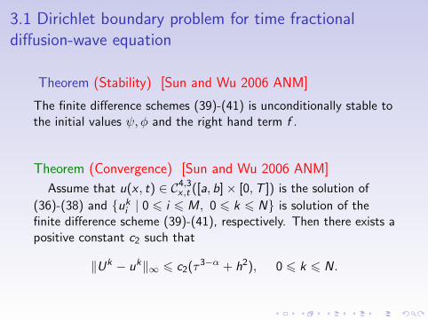
3.1 Dirichlet boundary problem for time fractionaldiffusion-wave equation
In 2006, we constructed the following second order and compactfinite difference schemes, respectively. i.e.,
Dατ u
k− 12
i = δ2xuk− 1
2i + f
k− 12
i , 1 6 i 6 M − 1, 1 6 k 6 N, (39)
u0i = ψ(xi ), 0 6 i 6 M, (40)
uk0 = ϕ1(tk), uk
M = ϕ2(tk), 1 6 k 6 N. (41)

3.1 Dirichlet boundary problem for time fractionaldiffusion-wave equation
Theorem (Stability) [Sun and Wu 2006 ANM]
The finite difference schemes (39)-(41) is unconditionally stable tothe initial values ψ, φ and the right hand term f .
Theorem (Convergence) [Sun and Wu 2006 ANM]
Assume that u(x , t) ∈ C4,3x ,t ([a, b]× [0,T ]) is the solution of
(36)-(38) and uki | 0 6 i 6 M, 0 6 k 6 N is solution of the
finite difference scheme (39)-(41), respectively. Then there exists apositive constant c2 such that
‖Uk − uk‖∞ 6 c2(τ3−α + h2), 0 6 k 6 N.

3.1 Dirichlet boundary problem for time fractionaldiffusion-wave equation
In 2010, we established the following spatial fourth order differencescheme
ADατ u
k− 12
i = δ2xuk− 1
2i +Af
k− 12
i , 1 6 i 6 M − 1, 1 6 k 6 N,(42)
u0i = ψ(xi ), 0 6 i 6 M, (43)
uk0 = ϕ1(tk), uk
M = ϕ2(tk), 1 6 k 6 N. (44)
We proved that

3.1 Dirichlet boundary problem for time fractionaldiffusion-wave equation
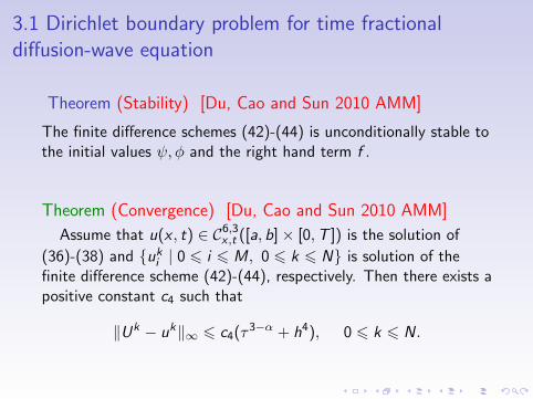
Theorem (Stability) [Du, Cao and Sun 2010 AMM]
The finite difference schemes (42)-(44) is unconditionally stable tothe initial values ψ, φ and the right hand term f .
Theorem (Convergence) [Du, Cao and Sun 2010 AMM]
Assume that u(x , t) ∈ C6,3x ,t ([a, b]× [0,T ]) is the solution of
(36)-(38) and uki | 0 6 i 6 M, 0 6 k 6 N is solution of the
finite difference scheme (42)-(44), respectively. Then there exists apositive constant c4 such that
‖Uk − uk‖∞ 6 c4(τ3−α + h4), 0 6 k 6 N.
3.1 Dirichlet boundary problem for time fractionaldiffusion-wave equation
Theorem (Stability) [Du, Cao and Sun 2010 AMM]
The finite difference schemes (42)-(44) is unconditionally stable tothe initial values ψ, φ and the right hand term f .
Theorem (Convergence) [Du, Cao and Sun 2010 AMM]
Assume that u(x , t) ∈ C6,3x ,t ([a, b]× [0,T ]) is the solution of
(36)-(38) and uki | 0 6 i 6 M, 0 6 k 6 N is solution of the
finite difference scheme (42)-(44), respectively. Then there exists apositive constant c4 such that
‖Uk − uk‖∞ 6 c4(τ3−α + h4), 0 6 k 6 N.

3.1 Dirichlet boundary problem for time fractionaldiffusion-wave equation
Table: Convergence order of difference scheme (42)-(44) in temporaldirection with h = 1
200 .
α τ e∞(h, τ) Order
α = 1.3 1/20 1.341e-4 ∗1/40 4.341e-5 1.62761/80 1.389e-5 1.64441/160 4.404e-6 1.6567
α = 1.5 1/20 4.544e-4 ∗1/40 1.656e-4 1.45581/80 5.979e-5 1.47001/160 2.144e-5 1.4794
α = 1.7 1/20 1.237e-3 ∗1/40 5.111e-4 1.27531/80 2.098e-4 1.28441/160 8.579e-5 1.2903

3.1 Dirichlet boundary problem for time fractionaldiffusion-wave equation
Table: Convergence order of difference scheme (42)-(44) in spatialdirection ( τ = 1
100000 , α = 1.5).
h e∞(h, τ) Order
1/2 4.4035e-3 *1/4 2.5365e-4 4.1181/8 1.5560e-5 4.0271/16 9.7010e-7 4.0041/32 6.2794e-8 3.949

3.2 Neumann boundary problem for time fractionaldiffusion-wave equation
Considering the following one-dimensional time fractionaldiffusion-wave equation
C0 Dα
t u(x , t) =∂2u(x , t)
∂x2+ f (x , t), a < x < b, 0 < t 6 T , (45)
u(x , 0) = ϕ(x),∂u(x , 0)
∂t= ψ(x), a 6 x 6 b, (46)
∂u(a, t)
∂x= 0,
∂u(b, t)
∂x= 0, 0 < t 6 T , (47)
where α ∈ (1, 2).

3.2 Neumann boundary problem for time fractionaldiffusion-wave equation
In 2013, we constructed the following spatial second orderdifference scheme
HDατ u
k− 12
i = δ2xuk− 1
2i +Hf
k− 12
i , 0 6 i 6 M, 1 6 k 6 N, (48)
u0i = ϕi , 0 6 i 6 M, (49)
where
Hui =
1
3(2u0 + u1), i = 0,
ui , 1 6 i 6 M − 1,
1
3(uM−1 + 2uM), i = M.
and the spatial fourth order finite difference scheme

3.2 Neumann boundary problem for time fractionaldiffusion-wave equation
BDατ u
k− 12
0 =2
hδxu
k− 12
12
+h
6(fx)
k− 12
0 − h3
90
[(fxxx)
k− 12
0 + (C0 Dαt fx)
k− 12
0
]+ Bf
k− 12
0 , 1 6 k 6 N, (50)
BDατ u
k− 12
i = δ2xuk− 1
2i + Bf
k− 12
i , 1 6 i 6 M − 1, 1 6 k 6 N,(51)
BDατ u
k− 12
M = −2
hδxu
k− 12
M− 12
− h
6(fx)
k− 12
M +h3
90
[(fxxx)
k− 12
M + (C0 Dαt fx)
k− 12
M
]+ Bf
k− 12
M , 1 6 k 6 N, (52)
u0i = ϕi , 0 6 i 6 M. (53)

3.2 Neumann boundary problem for time fractionaldiffusion-wave equation
Theorem (Stability) [ Ren and Sun 2013 JSC]
The finite difference schemes (48)-(49) and (50)-(53) are bothunconditionally stable to the initial values ψ,ϕ and the right handterm f .
Theorem (Convergence) [Ren and Sun 2013 JSC]
Assume that u(x , t) ∈ C4,3x ,t ([a, b]× [0,T ]) is the solution of
(45)-(47) and uki | 0 6 i 6 M, 0 6 k 6 N is solution of the
finite difference scheme (48)-(49), respectively. Then there exists apositive constant C such that
‖Uk − uk‖∞ 6 C (τ3−α + h2), 0 6 k 6 N.

3.2 Neumann boundary problem for time fractionaldiffusion-wave equation
Theorem (Convergence) [Ren and Sun 2013 JSC]
Assume that u(x , t) ∈ C6,3x ,t ([a, b]× [0,T ]) is the solution of
(45)-(47) and uki | 0 6 i 6 M, 0 6 k 6 N is solution of the
finite difference scheme (50)-(53), respectively. Then there exists apositive constant C such that
‖Uk − uk‖∞ 6 C (τ3−α + h4), 0 6 k 6 N.

3.2 Neumann boundary problem for time fractionaldiffusion-wave equation
In (45), let T = 1. In order to test the convergence rate of theproposed methods, we consider the exact solution of the problem(45)-(47) as follows
u(x , t) = exx2(1− x)2tγ+2.
Then it can be checked that the corresponding forcing term f (x , t)and initial conditions ϕ(x), ψ(x) are respectively
f (x , t) =Γ(γ + 3)
2t2exx2(1−x)2−ex tγ+2(2−8x +x2 +6x3 +x4),
andϕ(x) = 0, ψ(x) = 0.

3.2 Neumann boundary problem for time fractionaldiffusion-wave equation
Table: Convergence orders of scheme (48)-(49) and scheme (50)-(53) intemporal direction with h = 1
2000 .
scheme (48)-(49) scheme (50)-(53)α τ e∞(h, τ) Order e∞(h, τ) Order
1/10 1.148e-3 * 1.148e-3 *1/20 3.549e-4 1.694 3.547e-4 1.694
1.3 1/40 1.096e-4 1.695 1.095e-4 1.6961/80 3.392e-5 1.693 3.374e-5 1.6981/160 1.058e-5 1.681 1.039e-5 1.699
1/10 5.201e-3 * 5.201e-3 *1/20 2.096e-3 1.311 2.096e-3 1.311
1.7 1/40 8.499e-4 1.302 8.498e-4 1.3021/80 3.452e-4 1.300 3.452e-4 1.3001/160 1.403e-4 1.299 1.402e-4 1.299

3.2 Neumann boundary problem for time fractionaldiffusion-wave equation
Table: Convergence order of scheme (48)-(49) in spatial direction (τ = 1
2000 , α = 1.1).
h e∞(h, τ) Order
1/20 2.929e-3 *1/40 8.485e-4 1.7881/80 2.281e-4 1.8951/160 5.915e-5 1.9471/320 1.507e-5 1.973
Table: Convergence order of scheme (50)-(53) in spatial direction (τ = 1
10000 , α = 1.1).
h e∞(h, τ) Order
1/4 3.168e-3 *1/8 1.960e-4 4.0151/16 1.221e-5 4.0041/32 7.620e-7 4.0031/64 4.677e-8 4.026
3.2 Neumann boundary problem for time fractionaldiffusion-wave equation
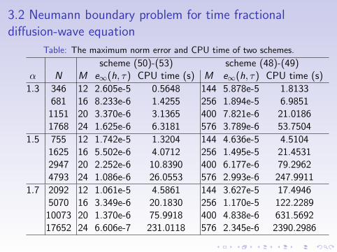
Table: The maximum norm error and CPU time of two schemes.
scheme (50)-(53) scheme (48)-(49)α N M e∞(h, τ) CPU time (s) M e∞(h, τ) CPU time (s)
1.3 346 12 2.605e-5 0.5648 144 5.878e-5 1.8133681 16 8.233e-6 1.4255 256 1.894e-5 6.98511151 20 3.370e-6 3.1365 400 7.821e-6 21.01861768 24 1.625e-6 6.3181 576 3.789e-6 53.7504
1.5 755 12 1.742e-5 1.3204 144 4.636e-5 4.51041625 16 5.502e-6 4.0712 256 1.495e-5 21.45312947 20 2.252e-6 10.8390 400 6.177e-6 79.29624793 24 1.086e-6 26.0553 576 2.993e-6 247.9911
1.7 2092 12 1.061e-5 4.5861 144 3.627e-5 17.49465070 16 3.349e-6 20.1830 256 1.170e-5 122.228910073 20 1.370e-6 75.9918 400 4.838e-6 631.569217652 24 6.606e-7 231.0118 576 2.345e-6 2390.2986

4. Multi-term time fractional diffusion-wave equation
Consider the following two-term time fractional mixeddiffusion-wave equation
C0 D
α1t u(x , t) + C
0 Dαt u(x , t) =
∂2u(x , t)
∂x2+ f (x , t),
0 < x < L, 0 < t 6 T , (54)
u(x , 0) = ϕ1(x), ut(x , 0) = ϕ2(x), 0 6 x 6 L, (55)
u(0, t) = ψ1(t), u(L, t) = ψ2(t), 0 < t 6 T , (56)
where 0 < α1 < 1 < α < 2, ϕ1(x), ϕ2(x), ψ1(t), ψ2(t) and f (x , t)are known smooth functions.

4. Multi-term time fractional diffusion-wave equationWe established the following spatial fourth order (compact)difference scheme
τ
2µ1A
( k∑j=1
aα1k−jδtu
j− 12
i +k−1∑j=1
aα1k−j−1δtu
j− 12
i
)+ADα
τ uk− 1
2i
= δ2xuk− 1
2i +Af
k− 12
i , 1 6 i 6 M − 1, 1 6 k 6 N, (57)
u0i = ϕ1(xi ), 0 6 i 6 M, (58)
uk0 = ψ1(tk), uk
M = ψ2(tk), 1 6 k 6 N. (59)
In (57), Auki = 1
12(uki−1 + 10uk
i + uki+1),
Dατ u
k− 12
i =1
µ0
[δtu
k− 12
i −k−1∑j=1
(bαk−j−1− bα
k−j)δtuj− 1
2i − bα
k−1ϕ2(xi )],
where µ0 = τα−1Γ(3− α), bαk = (k + 1)2−α − k2−α.
We have proved that

4. Multi-term time fractional diffusion-wave equation
Theorem (Stability) [Zhang, Sun]
The difference scheme (57)-(59) is unconditionally stable to theinitial values ϕ1(x) and ϕ2(x) and the right hand term f .
Theorem (Convergence) [Zhang, Sun]
Assume that u(x , t) ∈ C6,3x ,t ([0, L]× [0,T ]) is the solution of
(54)-(56) and uki | 0 6 i 6 M, 0 6 k 6 N is the solution of the
difference scheme (57)-(59), respectively. Then, for kτ 6 T , itholds that
‖ek‖∞ 6c1L
4
√6Γ(2− α)Tα(τmin2−α1,3−α + h4), 0 6 k 6 N.

4. Multi-term time fractional diffusion-wave equation
Let L = π,T = 1. We consider the exact solution of the problem(54)-(56) as follows
u(x , t) = t1+α1+α sin x .
Then it can be checked that the corresponding source term f (x , t),initial and boundary conditions are respectively
f (x , t) =(Γ(2 + α1 + α)
Γ(2 + α)t1+α+
Γ(2 + α1 + α)
Γ(2 + α1)t1+α1+t1+α1+α
)sin x ,
andϕ(x) = 0, ψ1(t) = 0, ψ2(t) = 0.

4. Multi-term time fractional diffusion-wave equation
Table: Numerical convergence of the difference scheme (57)-(59) intemporal direction with h = π
100 .
α1, α τ e∞(h, τ) Order1
α1 = 0.2, α = 1.7 1/10 4.145e-2 ∗1/20 1.707e-2 1.2801/40 6.969e-3 1.2931/80 2.833e-3 1.298
α1 = 0.3, α = 1.2 1/10 5.329e-3 ∗1/20 1.667e-3 1.6771/40 5.164e-4 1.6911/80 1.589e-4 1.700

4. Multi-term time fractional diffusion-wave equation
Table: Numerical convergence of the difference scheme (57)-(59) inspatial direction with τ = 1
200000 .
α1, α h e∞(h, τ) Order2
α1 = 0.1, α = 1.3 π/2 4.074e-3 ∗π/4 2.413e-4 4.078π/8 1.482e-5 4.025π/16 9.223e-7 4.006

5.1 ADI methods for 2D time fractional sub-diffusionequation
Consider the following two-dimensional time fractionalsub-diffusion equation
C0 Dα
t u(x , y , t) = ∆u(x , y , t) + f (x , y , t), (x , y) ∈ Ω, 0 < t 6 T ,(60)
u(x , y , 0) = ψ(x , y), (x , y) ∈ Ω = Ω ∪ ∂Ω, (61)
u(x , y , t) = ϕ(x , y , t), (x , y) ∈ ∂Ω, 0 < t 6 T , (62)
where 0 < α < 1, ∆ is the two-dimensional Laplacian operator, thedomain Ω = (0, L1)× (0, L2), and ∂Ω is the boundary,ϕ(x , y , t), ψ(x , y) and f (x , y , t) are known smooth functions.

5.1 ADI methods for 2D time fractional sub-diffusionequation
Taking two positive integers M1,M2, let xi = ih1 and yj = jh2 withh1 = L1/M1 and h2 = L2/M2. Define Ωh1 = xi | 0 6 i 6 M1 andΩh2 = yj | 0 6 j 6 M2, then the domain Ω is covered byΩh = Ωh1 × Ωh2 . For any mesh functionu = uij | 0 6 i 6 M1, 0 6 j 6 M2 defined on Ωh1 × Ωh2 , denote
δxui− 12,j =
1
h1(uij − ui−1,j), δyui ,j− 1
2=
1
h2(uij − ui ,j−1),
δ2xuij =1
h1
(δxui+ 1
2,j − δxui− 1
2,j
), δ2yuij =
1
h2
(δyui ,j+ 1
2− δyui ,j− 1
2
).
Axuij =
1
12(ui−1,j + 10uij + ui+1,j), 1 6 i 6 M1 − 1, 0 6 j 6 M2,
uij , i = 0 or M1, 0 6 j 6 M2,
Ayuij =
1
12(ui ,j−1 + 10uij + ui ,j+1), 1 6 j 6 M2 − 1, 0 6 i 6 M1,
uij , j = 0 or M2, 0 6 i 6 M1.
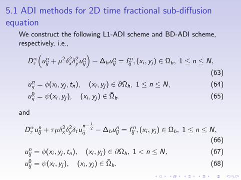
5.1 ADI methods for 2D time fractional sub-diffusionequation
We construct the following L1-ADI scheme and BD-ADI scheme,respectively, i.e.,
Dατ
(unij + µ2δ2xδ
2yun
ij
)−∆hu
nij = f n
ij , (xi , yj) ∈ Ωh, 1 ≤ n ≤ N,
(63)
unij = φ(xi , yj , tn), (xi , yj) ∈ ∂Ωh, 1 ≤ n ≤ N, (64)
u0ij = ψ(xi , yj), (xi , yj) ∈ Ωh. (65)
and
Dατ un
ij + τµδ2xδ2yδtu
n− 12
ij −∆hunij = f n
ij , (xi , yj) ∈ Ωh, 1 ≤ n ≤ N,
(66)
unij = φ(xi , yj , tn), (xi , yj) ∈ ∂Ωh, 1 < n ≤ N, (67)
u0ij = ψ(xi , yj), (xi , yj) ∈ Ωh. (68)

5.1 ADI methods for 2D time fractional sub-diffusionequation
Theorem (Stability) [Zhang and Sun 2011 JCP]
The finite difference schemes (63)-(65) and (66)-(68) areunconditionally stable to the initial value ψ and the right handterm f .
Theorem (Convergence) [Zhang and Sun 2011 JCP]
Assume that the problem (60)-(62) has smooth solutionu(x , y , t) in the domain Ω× [0,T ] andun
ij | (xi , yj) ∈ Ωh, 1 ≤ n ≤ N be the solution of the differenceschemes (63)-(65) and (66)-(68). Then there exists a positiveconstant C such that
|Un − un|H1 6 C (τmin2α,2−α + h21 + h2
2), 1 ≤ n ≤ N.√√√√τn∑
k=1
|Uk − uk |2H16 C (τmin1+α,2−α + h2
1 + h22), 1 ≤ n ≤ N.

5.1 ADI methods for 2D time fractional sub-diffusionequation
Theorem (Stability) [Zhang and Sun 2011 JCP]
The finite difference schemes (63)-(65) and (66)-(68) areunconditionally stable to the initial value ψ and the right handterm f .
Theorem (Convergence) [Zhang and Sun 2011 JCP]
Assume that the problem (60)-(62) has smooth solutionu(x , y , t) in the domain Ω× [0,T ] andun
ij | (xi , yj) ∈ Ωh, 1 ≤ n ≤ N be the solution of the differenceschemes (63)-(65) and (66)-(68). Then there exists a positiveconstant C such that
|Un − un|H1 6 C (τmin2α,2−α + h21 + h2
2), 1 ≤ n ≤ N.√√√√τ
n∑k=1
|Uk − uk |2H16 C (τmin1+α,2−α + h2
1 + h22), 1 ≤ n ≤ N.

5.1 ADI methods for 2D time fractional sub-diffusionequation
Table: Convergence order of (63)-(65) in temporal direction withh = π
200 .
α N e∞(τ, h) Order e∞(τ, h) Order
1/2 10 3.4910e-3 * 4.9026e-4 *20 1.9907e-3 0.8104 1.7394e-4 1.494940 1.0823e-3 0.8791 6.0359e-5 1.527080 5.7133e-4 0.9217 * *
2/3 10 1.4331e-3 * 4.0710e-5 *20 5.9327e-4 1.2724 1.1591e-5 1.812440 2.4243e-4 1.2911 4.4132e-6 1.393180 9.8870e-5 1.2940 * *
3/4 10 3.8502e-3 * 2.3582e-4 *20 1.7555e-3 1.1331 7.6934e-5 1.616040 7.8267e-4 1.1654 2.6593e-5 1.532680 3.4449e-4 1.1840 * *

5.1 ADI methods for 2D time fractional sub-diffusionequation
Table: Convergence orders of scheme (66)-(68) in temporal directionwith h = π
200 .
α N e∞(τ, h) Order e∞(τ, h) Order
1/3 10 3.8684e-3 * 1.8001e-4 *20 1.6437e-3 1.2347 4.5085e-5 1.997340 6.7951e-4 1.2744 1.1695e-5 1.946780 2.7672e-4 1.2961 * *
1/2 10 8.8067e-4 * 2.1851e-5 *20 3.2549e-4 1.4360 1.7096e-6 3.676040 1.1618e-4 1.4862 6.1627e-7 1.472180 4.0678e-5 1.5141 * *
2/3 10 2.2326e-3 * 2.1368e-4 *20 1.0149e-3 1.1374 6.8734e-5 1.636440 4.4422e-4 1.1920 2.1960e-5 1.646180 1.8953e-4 1.2288 * *

5.1 ADI methods for 2D time fractional sub-diffusionequation
Table: Convergence orders in spatial direction ( τ = 12000 , α = 0.5).
M e∞(τ, h) Order
difference scheme(63)-(65) 4 5.1273e-3 *8 1.2844e-3 1.997216 3.2219e-4 1.995132 8.1568e-5 1.9818
difference scheme (66)-(68) 4 6.0514e-3 *8 1.5096e-3 2.003116 3.7696e-4 2.001732 9.3984e-5 2.0039

5.2 ADI methods for 2D time fractional diffusion-waveequation
Consider the following two-dimensional time fractionaldiffusion-wave equation
C0 D
γt u(x , y , t) = ∆u(x , y , t) + f (x , y , t), (x , y) ∈ Ω, 0 < t 6 T ,
(69)
u(x , y , 0) = ψ(x , y), ut(x , y , 0) = φ(x , y), (x , y) ∈ Ω = Ω ∪ ∂Ω,(70)
u(x , y , t) = ϕ(x , y , t), (x , y) ∈ ∂Ω, 0 < t 6 T , (71)
where 1 < γ < 2, ∆ is the two-dimensional Laplacian operator, thedomain Ω = (0, L1)× (0, L2), and ∂Ω is the boundary,ϕ(x , y , t), ψ(x , y), φ(x , y) and f (x , y , t) are known smoothfunctions.

5.2 ADI methods for 2D time fractional diffusion-waveequation
We constructed the following Crank-Nicolson scheme
Dγτ u
n− 12
ij = ∆hun− 1
2ij − Γ(3− γ)
4τ1+γδ2xδ
2yδtu
n− 12
ij + fn− 1
2ij ,
(xi , yj) ∈ Ωh, 1 ≤ n ≤ N, (72)
unij = φ(xi , yj , tn), (xi , yj) ∈ ∂Ωh, 1 ≤ n ≤ N, (73)
u0ij = ψ(xi , yj), (xi , yj) ∈ Ωh. (74)
The difference scheme (72) can be decomposed into the ADI form.

5.2 ADI methods for 2D time fractional diffusion-waveequation
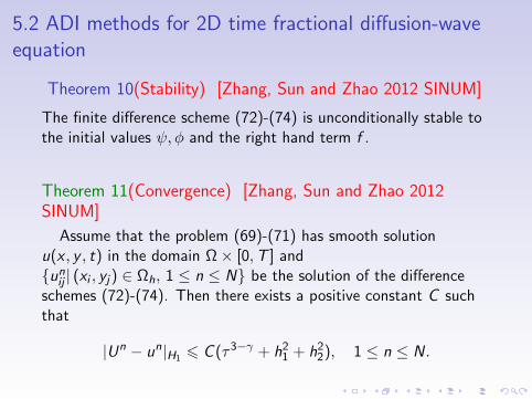
Theorem 10(Stability) [Zhang, Sun and Zhao 2012 SINUM]
The finite difference scheme (72)-(74) is unconditionally stable tothe initial values ψ, φ and the right hand term f .
Theorem 11(Convergence) [Zhang, Sun and Zhao 2012SINUM]
Assume that the problem (69)-(71) has smooth solutionu(x , y , t) in the domain Ω× [0,T ] andun
ij | (xi , yj) ∈ Ωh, 1 ≤ n ≤ N be the solution of the differenceschemes (72)-(74). Then there exists a positive constant C suchthat
|Un − un|H1 6 C (τ3−γ + h21 + h2
2), 1 ≤ n ≤ N.
5.2 ADI methods for 2D time fractional diffusion-waveequation
Theorem 10(Stability) [Zhang, Sun and Zhao 2012 SINUM]
The finite difference scheme (72)-(74) is unconditionally stable tothe initial values ψ, φ and the right hand term f .
Theorem 11(Convergence) [Zhang, Sun and Zhao 2012SINUM]
Assume that the problem (69)-(71) has smooth solutionu(x , y , t) in the domain Ω× [0,T ] andun
ij | (xi , yj) ∈ Ωh, 1 ≤ n ≤ N be the solution of the differenceschemes (72)-(74). Then there exists a positive constant C suchthat
|Un − un|H1 6 C (τ3−γ + h21 + h2
2), 1 ≤ n ≤ N.

5.2 ADI methods for 2D time fractional diffusion-waveequation
We presented the following compact scheme
AxAyDγτ u
n− 12
ij = (Ayδ2x +Axδ
2y )u
n− 12
ij − Γ(3− γ)
4τ1+γδ2xδ
2yδtu
n− 12
ij
+AxAy fn− 1
2ij , (xi , yj) ∈ Ωh, 1 ≤ n ≤ N, (75)
unij = φ(xi , yj , tn), (xi , yj) ∈ ∂Ωh, 1 ≤ n ≤ N, (76)
u0ij = ψ(xi , yj), (xi , yj) ∈ Ωh. (77)
The difference scheme (75) can be decomposed into the ADI form.

5.2 ADI methods for 2D time fractional diffusion-waveequation
Theorem 12(Stability) [Zhang, Sun and Zhao 2012 SINUM]
The finite difference scheme (75)-(77) is unconditionally stable tothe initial values ψ, φ and the right hand term f .
Theorem 13(Convergence) [Zhang, Sun and Zhao 2012SINUM]
Assume that the problem (69)-(71) has smooth solutionu(x , y , t) in the domain Ω× [0,T ] andun
ij | (xi , yj) ∈ Ωh, 1 ≤ n ≤ N be the solution of the differencescheme (75)-(77). Then there exists a positive constant C suchthat
|Un − un|H1 6 C (τ3−γ + h41 + h4
2), 1 ≤ n ≤ N.

5.2 ADI methods for 2D time fractional diffusion-waveequation
In (36)-(38), let Ω = (0, π)× (0, π),
f (x , y , t) = sin x sin y[Γ(3 + γ)
2t2 − 2t2−γ
],
u(x , y , 0) = 0, ut(x , y , 0) = 0, ϕ(x , y , t) = 0.Then the exact solution is
u(x , y , t) = sin x sin y t2−γ .

5.2 ADI methods for 2D time fractional diffusion-waveequation
Table: Convergence order of difference scheme (72)-(74) in temporaldirection with h = π
200 .
scheme (72)-(74) scheme (75)-(77)γ τ e∞(h, τ) Order e∞(h, τ) Order
1/5 2.7052e-2 ∗ 2.7048e-2 ∗1/10 8.4520e-3 1.6784 8.4482e-3 1.6788
1.25 1/20 2.5914e-3 1.7056 2.5877e-3 1.70701/40 7.8867e-4 1.7162 7.8500e-4 1.72091/80 2.4108e-4 1.7099 2.3742e-4 1.7253
1/5 1.9341e-1 ∗ 1.9340e-1 ∗1/10 8.1579e-2 1.2454 8.1577e-2 1.2454
1.75 1/20 3.4381e-2 1.2466 3.4379e-2 1.24661/40 1.4485e-2 1.2470 1.4484e-2 1.24711/80 6.1002e-3 1.2477 6.0986e-3 1.2479

5.2 ADI methods for 2D time fractional diffusion-waveequation
Table: Convergence order scheme (72)-(74) in spatial direction (γ = 1.1).
h e∞(τ, h) Order
scheme (72)-(74) π/4 1.5865e-2 ∗scheme (τ = 1/1000) π/8 3.9882e-3 1.9921
π/16 9.9877e-4 1.9975π/32 2.5019e-4 1.9971
scheme (75)-(77) π/4 5.0632e-4 ∗scheme (τ = 1/10000) π/8 3.1104e-5 4.0249
π/16 1.9421e-6 4.0014π/32 1.2814e-7 3.9218

5.2 ADI methods for 2D time fractional diffusion-waveequation
Table: The maximum norm error and CPU time of two schemes.
scheme (75)-(77) scheme (72)-(74)γ N M e∞(τ, h) CPU time(s) M e∞(τ, h) CPU time(s)
1.25 24 4 2.1782e-3 0.0470 16 2.5190e-3 0.265060 6 4.5846e-4 0.4220 36 5.3406e-4 3.4380116 8 1.4733e-4 1.7190 64 1.7218e-4 21.4370193 10 6.0965e-5 5.6250 100 7.1313e-5 91.0620
1.5 40 4 3.9333e-3 0.1100 16 4.1774e-3 0.4530118 6 8.0156e-4 0.9060 36 8.5395e-4 6.8910256 8 2.5323e-4 5.0780 64 2.7022e-4 50.7810464 10 1.0412e-4 20.7810 100 1.1115e-4 252.4060
1.75 84 4 5.7572e-3 0.2340 16 5.9206e-3 0.9370309 6 1.1535e-3 3.5320 36 1.1872e-3 19.5630776 8 3.6654e-4 30.2970 64 3.7736e-4 197.95301585 10 1.5035e-4 178.5930 100 1.5480e-4 1680.1100

6. Conclusion
In this review, I report some works on the difference method forthe time fractional differential equations. At first, two discretefractional numerical differential formulae with their truncationerrors are presented. Then some difference schemes areconstructed for the Dirichlet problem, Neumann problem of thesubdiffusion equation and diffusion-wave equation, respectively.For the 2d problem, we concentrate on the ADI schemes. At lastthe multi term problems are considered. Both spatial second orderand fourth order difference schemes are established for eachproblem. The stability and convergence of the difference schemesare proved. The main tool for analyzing the difference schemes isthe energy method. Some numerical examples are provided andthe numerical results are accordance with the theoretical results.

References
Jincheng Ren, Zhi-zhong Sun, Numerical algorithm with high spatialaccuracy for the fractional diffusion-wave equation with Neumannboundary conditions, J Sci Comput., Published online: 20 January 2013
Guang-hua Gao, Zhi-zhong Sun, The finite difference approximation for aclass of fractional sub-diffusion equations on a space unbounded domain,Journal of Computational Physics, 236 (2013) 443-460
Jincheng Ren, Zhi-zhong Sun, Xuan Zhao, Compact difference schemefor the fractional sub-diffusion equation with Neumann boundaryconditions, Journal of Computational Physics, 232 (2013) 456-467
Ya-nan Zhang, Zhi-zhong Sun, and Xuan Zhao. Compact AlternatingDirection Implicit Scheme for the Two-Dimensional FractionalDiffusion-Wave Equation. SIAM J. Numer. Anal., 2012, 50, 1535-1555

Guang-hua Gao, Zhi-zhong Sun, Ya-nan Zhang, A finite differencescheme for fractional sub-diffusion equations on an unbounded domainusing artificial boundary conditions, Journal of Computational Physics231£7¤(2012), 2865-2879
Guang-hua Gao, Zhi-zhong Sun, A Finite Difference Approach for theInitial-Boundary Value Problem of the Fractional Klein-Kramers Equationin Phase Space, Cent. Eur. J. Math., 2012, 10(1), 101-115
Ya-nan Zhang, Zhi-zhong Sun, Alternating direction implicit schemes forthe two-dimensional fractional sub-diffusion equation, Journal ofComputational Physics 230 (24)(2011), 8713-8728
Ya-nan Zhang, Zhi-zhong Sun, Hong-wei Wu, Error estimates ofCrank-Nicolson type difference schemes for the sub-diffusion equation,SIAM J. Numer. Anal. 49 (2011), no. 6, 2302–2322.
Xuan Zhao, Zhi-zhong Sun, box-type scheme for fractional sub-diffusionequation with Neumann boundary conditions, Journal of ComputationalPhysics 230£15¤(2011), pp. 6061-6074
Guang-hua Gao, Zhi-zhong Sun, A compact finite difference scheme forthe fractional sub-diffusion equations, Journal of Computational Physics,230 £3¤(2011), 586-595
R. Du, W.R. Cao, Z.Z. Sun, A compact difference scheme for thefractional diffusion wave equation, Appl. Math. Modelling 34£10¤(Oct.2010), 2998-3007
Zhi-zhong Sun, Xiaonan Wu, A fully discrete difference scheme for adiffusion-wave system. Appl. Numer. Math. 56 (2006), no. 2, 193–209.
Xiaonan Wu, Zhi-Zhong Sun, Convergence of difference scheme for heatequation in unbounded domains using artificial boundary conditions.Appl. Numer. Math. 50 (2004), no. 2, 261–277.

Thanks for your attention!


![Approximate Lie Group Analysis of Finite–difference Equations · Approximate Lie Group Analysis of Finite–difference Equations A.M.Latypov ... Levi and Winternitz [8] applied](https://img.dokumen.tips/doc/110x75/5edcb4acad6a402d66677c2b/approximate-lie-group-analysis-of-finiteadiierence-equations-approximate-lie.jpg)