Finite Anticlastic Bending of Hyperelastic Solids and · PDF fileFinite Anticlastic Bending of Hyperelastic ... on the strain according to the linearized theory ... Anticlastic Bending

J Elast (2018) 131:137–170DOI 10.1007/s10659-017-9649-y

Finite Anticlastic Bending of Hyperelastic Solidsand Beams

Luca Lanzoni1 · Angelo Marcello Tarantino2

Received: 4 November 2016 / Published online: 30 June 2017© The Author(s) 2017. This article is published with open access at Springerlink.com

Abstract This paper deals with the equilibrium problem in nonlinear elasticity of hyper-elastic solids under anticlastic bending. A three-dimensional kinematic model, where thelongitudinal bending is accompanied by the transversal deformation of cross sections, isformulated. Following a semi-inverse approach, the displacement field prescribed by theabove kinematic model contains three unknown parameters. A Lagrangian analysis is per-formed and the compressible Mooney-Rivlin law is assumed for the stored energy function.Once evaluated the Piola-Kirchhoff stresses, the free parameters of the kinematic model aredetermined by using the equilibrium equations and the boundary conditions. An Euleriananalysis is then accomplished to evaluating stretches and stresses in the deformed config-uration. Cauchy stress distributions are investigated and it is shown how, for wide rangesof constitutive parameters, the obtained solution is quite accurate. The whole formulationproposed for the finite anticlastic bending of hyperelastic solids is linearized by introduc-ing the hypothesis of smallness of the displacement and strain fields. With this linearizationprocedure, the classical solution for the infinitesimal bending of beams is fully recovered.

Keywords Finite elasticity · Hyperelasticity · Equilibrium · Solids · Beams · Anticlasticbending

Mathematics Subject Classification 74B20

1 Introduction

The flexure of an elastic body is a classical problem of elastostatics that has been widelyinvestigated in literature because of its great relevance in many practical tasks. The majority

B L. [email protected]

A.M. [email protected]

1 DESD, Università di San Marino, via Salita alla Rocca 44, 47890 San Marino città, San Marino

2 DIEF, Università di Modena e Reggio Emilia, via Vignolese 905, 41125 Modena, Italy

http://crossmark.crossref.org/dialog/?doi=10.1007/s10659-017-9649-y&domain=pdf

http://orcid.org/0000-0002-3513-0273

mailto:[email protected]

mailto:[email protected]

138 L. Lanzoni, A.M. Tarantino

of studies has been performed by assuming infinitesimal strains and small displacementsof the body under bending (see, among the others, Bernoulli Jacob [1], Bernoulli Jacques[2], Parent [3], Euler [4–7], Navier [8], Barré de Saint Venant [9], Bresse [10], Lamb [11],Kelvin and Tait [12] and Love [13]).

One of the first investigations dealing with the above equilibrium problem in the frame-work of finite elasticity was carried out by Seth [14], who studied a plate under flexure inthe absence of body forces. Based on the semi-inverse method, he assumed the deformedconfiguration of the plate like a circular cylindrical shell, keeping valid the Bernoulli-Navierhypothesis for cross sections and assuming a linear dependence for the displacement field.Moreover, he assumed that the stress depends on the strain according to the linearized theoryof elasticity. In his work, the bending couples needed to induce the hypothesized configura-tion of the plate together with the position of the unstretched fibers within the plate thickness(neutral axis) were also assessed.

The flexion problem of an elastic block has been studied by Rivlin [15], considering thedeformation that transforms the elastic block into a cylinder having the base in the shapeof a circular crown sector. No displacements along the axis of the cylinder have been takeninto account, making the problem as a matter of fact two-dimensional. Surface tractionsnecessary to induced the assumed displacement field have been determined, showing that inthe case of an incompressible neo-Hookean material, these surface tractions are equivalentto two equal and opposite couples acting at the end faces. Subsequently, Rivlin generalizedhis study formulating the equilibrium problem without specifying the form of the storedenergy function [16].

Shield [17] investigated the problem of a beam under pure bending by assuming smallstrain but large displacements. He retrieves the Lamb’s solution [11] for the deflection ofthe middle surface of the beam. As remarked in that work, for large values of the width-to-thickness ratios, the deflection profile is flat in the central portion of the cross section andoscillatory near the edges.

A closed-form solution of a compressible rectangular body made of Hencky material un-der finite plane bending has been obtained by Bruhns et al. [18], giving explicit relationshipsfor the bending angle and bending moment as functions of the circumferential stretch.

It is important to note that all the aforementioned works address the bending problemin a two-dimensional context, neglecting systematically the deformation in the directionperpendicular to the inflexion plane. Proceeding in this way, the modeling is simplifiedsubstantially, since the displacement field is assumed to be plane, renouncing to describea phenomenon which in reality is purely three-dimensional. In particular, the transversaldeformation, always coupled with the longitudinal inflexion of a solid, is known as the anti-clastic effect.

This paper presents a fully nonlinear analysis of solids under anticlastic bending. Inthe next section, a three-dimensional kinematic model, where the longitudinal bending isaccompanied by the transversal deformation of cross sections, is formulated by introduc-ing three basic hypotheses. Following a semi-inverse approach, the displacement field pre-scribed by the kinematic model contains three unknown parameters. In Sect. 3, a Lagrangiananalysis is performed and the compressible Mooney-Rivlin law is assumed for the storedenergy function. Once evaluated the Piola-Kirchhoff stresses, the free parameters of thekinematic model are determined by using the equilibrium equations and the boundary con-ditions. With the purpose of evaluating stretches and stresses in the deformed configuration,an Eulerian analysis is accomplished in Sect. 4. Cauchy stress distributions are investigatedand intervals for the constitutive parameters, in which the solution is particularly accurate,are established. The whole formulation proposed for the finite anticlastic bending of hy-perelastic solids is linearized in Sect. 5, by introducing the hypothesis of smallness of the

Finite Anticlastic Bending of Hyperelastic Solids and Beams 139

displacement and strain fields. With this linearization procedure, the classical solution forthe infinitesimal bending of beams is fully recovered.

2 Kinematics

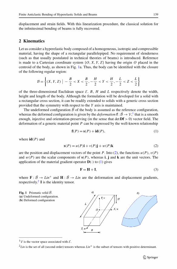
Let us consider a hyperelastic body composed of a homogeneous, isotropic and compressiblematerial, having the shape of a rectangular parallelepiped. No requirement of slenderness(such as that usually postulated in technical theories of beams) is introduced. Referenceis made to a Cartesian coordinate system {O,X,Y,Z} having the origin O placed in thecentroid of the body, as shown in Fig. 1a. Thus, the body can be identified with the closureof the following regular region:

B ={(X,Y,Z)

∣∣ − B

2< X <

B

2,−H

2< Y <

H

2,−L

2< Z <

L

2

}

of the three-dimensional Euclidean space E . B , H and L respectively denote the width,height and length of the body. Although the formulation will be developed for a solid witha rectangular cross section, it can be readily extended to solids with a generic cross sectionprovided that the symmetry with respect to the Y axis is maintained.

The undeformed configuration B of the body is assumed as the reference configuration,whereas the deformed configuration is given by the deformation f : B → V ,1 that is a smoothenough, injective and orientation-preserving (in the sense that det Df > 0) vector field. Thedeformation of a generic material point P can be expressed by the well-known relationship

f(P ) = s(P ) + id(P ), (1)

where id(P ) and

s(P ) = u(P )i + v(P )j + w(P )k (2)

are the position and displacement vectors of the point P . Into (2), the functions u(P ), v(P )

and w(P ) are the scalar components of s(P ), whereas i, j and k are the unit vectors. Theapplication of the material gradient operator D(·) to (1) gives

F = H + I, (3)

where F : B → Lin+ and H : B → Lin are the deformation and displacement gradients,respectively.2 I is the identity tensor.

Fig. 1 Prismatic solid B.(a) Undeformed configuration.(b) Deformed configuration

1V is the vector space associated with E .2Lin is the set of all (second order) tensors whereas Lin+ is the subset of tensors with positive determinant.


Fixed notation, hereinafter the formulation of the equilibrium problem of an inflexedsolid will be performed. Solving such a problem means getting the displacement field. But,in general, this direct computation is a daunting task. Thus, to simplify the problem, somehypotheses, more or less based on the physical behavior of the solid, are generally postulatedin the literature. In this work, the three-dimensionality of the problem is maintained, withoutrenouncing to study none of the three components of the displacement field.3 This allows toexamine, in addition to the longitudinal inflexion along the Z axis of the solid, also the de-formation of cross sections, which are initially parallel to the XY plane. As show experimen-tal evidences (see, e.g., [19] and [20]) the solid transversely undergoes a second inflexion,whose sign is opposite to that longitudinal, known as anticlastic effect. Although the longi-tudinal curvature is generally larger, the two curvatures may have comparable magnitudes.

Taking into account the above considerations, the displacement field will be partially de-fined by adopting a semi-inverse approach. To this aim, the following three basic hypothesesare introduced.

1. The solid is inflexed longitudinally with constant curvature. Namely, each rectilinearsegment of the solid, parallel to the Z axis, is transformed into an arc of circumference.

2. Plane cross sections, orthogonal to the Z axis, remain as such after the solid has beeninflexed. Cross sections can deform only in their own plane and all in the same way.

3. As a result of longitudinal inflexion, the solid is inflexed also transversally with con-stant curvature, in such a way that any horizontal plane of the solid is transformed into atoroidal open surface.

The longitudinal inflexion can be thought of as generated by the application of a pairof self-balanced bending moments or by a geometric boundary condition which imposes aprescribed relative rotation between the two end faces of the solid.

In this paper, on the basis of the three previous assumptions, a kinematic model con-taining some unknown deformation parameters is derived. The model describes the dis-placement field (2) of the solid and it is the outcome of coupled effects generated by thelongitudinal and transversal curvatures. Through this kinematic model and relationship (1),the shape assumed by the solid in the deformed configuration is obtained (cf. Fig. 1b).

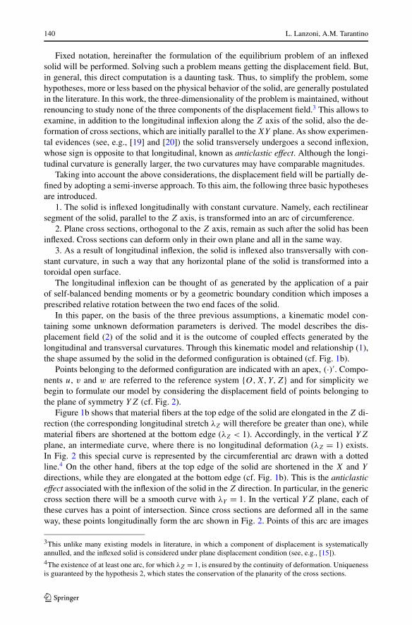
Points belonging to the deformed configuration are indicated with an apex, (·)′. Compo-nents u, v and w are referred to the reference system {O,X,Y,Z} and for simplicity webegin to formulate our model by considering the displacement field of points belonging tothe plane of symmetry YZ (cf. Fig. 2).

Figure 1b shows that material fibers at the top edge of the solid are elongated in the Z di-rection (the corresponding longitudinal stretch λZ will therefore be greater than one), whilematerial fibers are shortened at the bottom edge (λZ < 1). Accordingly, in the vertical YZ

plane, an intermediate curve, where there is no longitudinal deformation (λZ = 1) exists.In Fig. 2 this special curve is represented by the circumferential arc drawn with a dottedline.4 On the other hand, fibers at the top edge of the solid are shortened in the X and Y

directions, while they are elongated at the bottom edge (cf. Fig. 1b). This is the anticlasticeffect associated with the inflexion of the solid in the Z direction. In particular, in the genericcross section there will be a smooth curve with λY = 1. In the vertical YZ plane, each ofthese curves has a point of intersection. Since cross sections are deformed all in the sameway, these points longitudinally form the arc shown in Fig. 2. Points of this arc are images

3This unlike many existing models in literature, in which a component of displacement is systematicallyannulled, and the inflexed solid is considered under plane displacement condition (see, e.g., [15]).4The existence of at least one arc, for which λZ = 1, is ensured by the continuity of deformation. Uniquenessis guaranteed by the hypothesis 2, which states the conservation of the planarity of the cross sections.


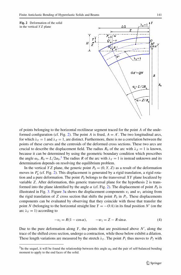
Fig. 2 Deformation of the solidin the vertical YZ plane

of points belonging to the horizontal rectilinear segment traced for the point A of the unde-formed configuration (cf. Fig. 2). The point A is fixed, A = A′. The two longitudinal arcs,for which λY = 1 and λZ = 1, are distinct. Furthermore, there is no a correlation between thepoints of these curves and the centroids of the deformed cross sections. These two arcs arecrucial to describe the displacement field. The radius R0 of the arc with λZ = 1 is known,because it can be determined by using the geometric boundary condition which prescribesthe angle α0, R0 = L/2α0.5 The radius R of the arc with λY = 1 is instead unknown and itsdetermination depends on resolving the equilibrium problem.

In the vertical YZ plane, the generic point P0 = (0, Y,Z) as a result of the deformationmoves in P ′

0 (cf. Fig. 2). This displacement is generated by a rigid translation, a rigid rota-tion and a pure deformation. The point P0 belongs to the transversal XY plane localized byvariable Z. After deformation, this generic transversal plane for the hypothesis 2 is trans-formed into the plane identified by the angle α (cf. Fig. 2). The displacement of point P0 isillustrated in Fig. 3. Figure 3a shows the displacement components v1 and w1 arising fromthe rigid translation of Z cross section that shifts the point P0 in P1. These displacementscomponents can be evaluated by observing that they coincide with those that transfer thepoint N (belonging to the horizontal straight line Y = −OA) in its final position N ′ (on thearc λY = 1) according to

−v1 = R(1 − cosα), −w1 = Z − R sinα. (4)

Due to the pure deformation along Y , the points that are positioned above N ′, along thetrace of the shifted cross section, undergo a contraction, while those below exhibit a dilation.These length variations are measured by the stretch λY . The point P1 thus moves to P2 with

5In the sequel, it will be found the relationship between this angle α0 and the pair of self-balanced bendingmoment to apply to the end faces of the solid.


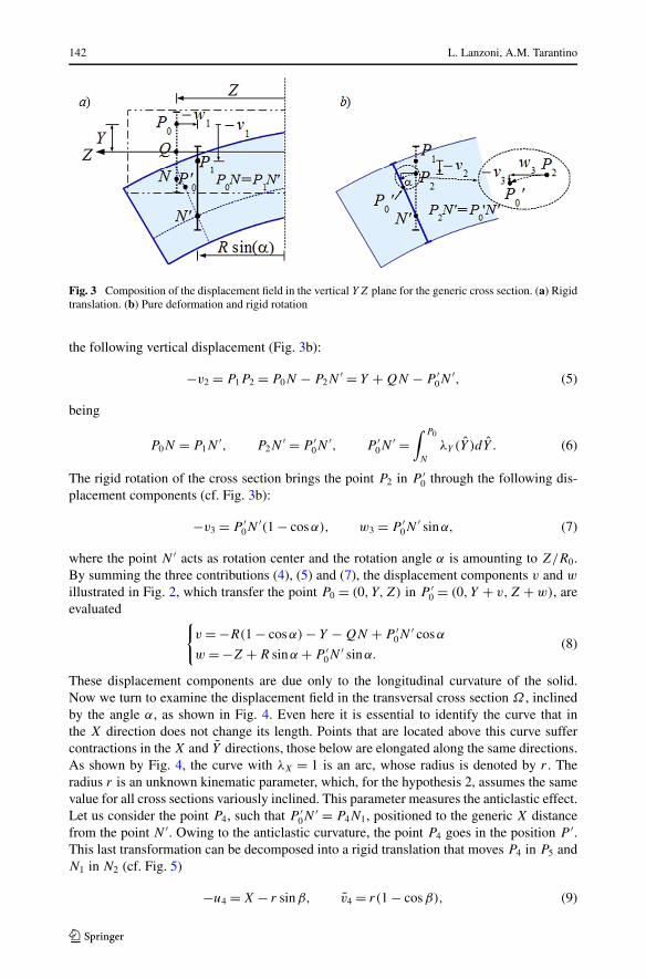
Fig. 3 Composition of the displacement field in the vertical YZ plane for the generic cross section. (a) Rigidtranslation. (b) Pure deformation and rigid rotation

the following vertical displacement (Fig. 3b):

−v2 = P1P2 = P0N − P2N′ = Y + QN − P ′

0N′, (5)

being

P0N = P1N′, P2N

′ = P ′0N

′, P ′0N

′ =∫ P0

N

λY (Y )dY . (6)

The rigid rotation of the cross section brings the point P2 in P ′0 through the following dis-

placement components (cf. Fig. 3b):

−v3 = P ′0N

′(1 − cosα), w3 = P ′0N

′ sinα, (7)

where the point N ′ acts as rotation center and the rotation angle α is amounting to Z/R0.By summing the three contributions (4), (5) and (7), the displacement components v and w

illustrated in Fig. 2, which transfer the point P0 = (0, Y,Z) in P ′0 = (0, Y + v,Z + w), are

evaluated {v = −R(1 − cosα) − Y − QN + P ′

0N′ cosα

w = −Z + R sinα + P ′0N

′ sinα.(8)

These displacement components are due only to the longitudinal curvature of the solid.Now we turn to examine the displacement field in the transversal cross section Ω , inclinedby the angle α, as shown in Fig. 4. Even here it is essential to identify the curve that inthe X direction does not change its length. Points that are located above this curve suffercontractions in the X and Y directions, those below are elongated along the same directions.As shown by Fig. 4, the curve with λX = 1 is an arc, whose radius is denoted by r . Theradius r is an unknown kinematic parameter, which, for the hypothesis 2, assumes the samevalue for all cross sections variously inclined. This parameter measures the anticlastic effect.Let us consider the point P4, such that P ′

0N′ = P4N1, positioned to the generic X distance

from the point N ′. Owing to the anticlastic curvature, the point P4 goes in the position P ′.This last transformation can be decomposed into a rigid translation that moves P4 in P5 andN1 in N2 (cf. Fig. 5)

−u4 = X − r sinβ, v4 = r(1 − cosβ), (9)


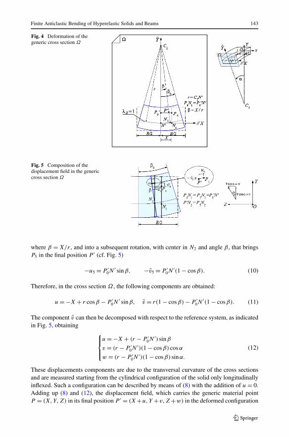
Fig. 4 Deformation of thegeneric cross section Ω

Fig. 5 Composition of thedisplacement field in the genericcross section Ω

where β = X/r , and into a subsequent rotation, with center in N2 and angle β , that bringsP5 in the final position P ′ (cf. Fig. 5)

−u5 = P ′0N

′ sinβ, −v5 = P ′0N

′(1 − cosβ). (10)

Therefore, in the cross section Ω , the following components are obtained:

u = −X + r cosβ − P ′0N

′ sinβ, v = r(1 − cosβ) − P ′0N

′(1 − cosβ). (11)

The component v can then be decomposed with respect to the reference system, as indicatedin Fig. 5, obtaining

⎧⎪⎨⎪⎩

u = −X + (r − P ′0N

′) sinβ

v = (r − P ′0N

′)(1 − cosβ) cosα

w = (r − P ′0N

′)(1 − cosβ) sinα.

(12)

These displacements components are due to the transversal curvature of the cross sectionsand are measured starting from the cylindrical configuration of the solid only longitudinallyinflexed. Such a configuration can be described by means of (8) with the addition of u = 0.Adding up (8) and (12), the displacement field, which carries the generic material pointP = (X,Y,Z) in its final position P ′ = (X+u,Y +v,Z+w) in the deformed configuration


of the solid, is achieved⎧⎪⎪⎪⎨⎪⎪⎪⎩

u = −X + (r − P ′0N

′) sin Xr

v = −R(1 − cos ZR0

) − Y − QN + P ′0N

′ cos ZR0

+ (r − P ′0N

′)(1 − cos Xr) cos Z

R0

w = −Z + (R + P ′0N

′) sin ZR0

+ (r − P ′0N

′)(1 − cos Xr) sin Z

R0.

(13)

In the above displacement field, an expression can be attributed to the segment P ′0N

′. Toassess the integral expression of P ′

0N′ = ∫ P0

NλY (Y )dY , the following relationship due to the

isotropy property6 of the solid can be used:

λX = λY . (14)

In order to evaluated these stretches it is useful to recall the definition of right Cauchy-Greenstrain tensor C and of left Cauchy-Green strain tensor B

C = FT F = UR−1RU = U2, B = FFT = RUUR−1 = RU2R−1, (15)

where the two tensors R and U are obtained by the polar decomposition of the deformationgradient F = RU. R is a proper orthogonal tensor and denotes the rotation tensor, whereasU is a symmetric and positive definite tensor that indicates the right stretch tensor. For thestate of deformation derived from (13), tensor U is diagonal, because the reference system{O,X,Y,Z} is principal. Diagonal components of U are the principal stretches. Therefore,the diagonal components of C are7

C11 = F 211 + F 2

21 + F 231 = λ2

X,

C22 = F 212 + F 2

22 + F 232 = λ2

Y ,

C33 = F 213 + F 2

23 + F 233 = λ2

Z.

(16)

Using (3) and computing the derivatives of the displacement field (13), equations (16) pro-vide the following expressions for the stretches:

⎧⎪⎪⎪⎨⎪⎪⎪⎩

λX = r−P ′0N ′

r

λY = ∂P ′0N ′

∂Y

λZ = RR0

+ P ′0N ′R0

+ (r−P ′0N ′)(1−cosβ)

R0,

(17)

taking into account that stretches are strictly positive quantities. The condition (14) can nowbe set by equating the first two expressions of (17). In this way, the following differentialequation is derived:

r∂(P ′

0N′)

∂Y+ P ′

0N′ − r = 0, (18)

whose solution is

P ′0N

′ = r − e− 1r (Y+QN)−C1 . (19)

6It is assumed that the isotropy property is preserved in the deformed configuration.7The other components of tensor C are zero.


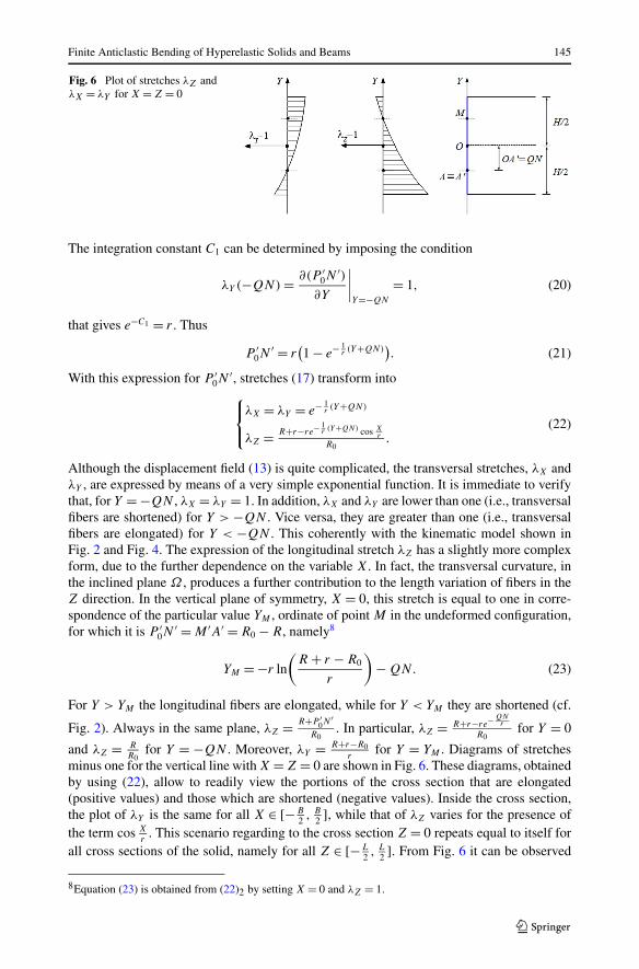
Fig. 6 Plot of stretches λZ andλX = λY for X = Z = 0

The integration constant C1 can be determined by imposing the condition

λY (−QN) = ∂(P ′0N

′)∂Y

∣∣∣∣Y=−QN

= 1, (20)

that gives e−C1 = r . Thus

P ′0N

′ = r(1 − e− 1

r (Y+QN)). (21)

With this expression for P ′0N

′, stretches (17) transform into⎧⎨⎩

λX = λY = e− 1r (Y+QN)

λZ = R+r−re− 1r (Y+QN) cos X

r

R0.

(22)

Although the displacement field (13) is quite complicated, the transversal stretches, λX andλY , are expressed by means of a very simple exponential function. It is immediate to verifythat, for Y = −QN , λX = λY = 1. In addition, λX and λY are lower than one (i.e., transversalfibers are shortened) for Y > −QN . Vice versa, they are greater than one (i.e., transversalfibers are elongated) for Y < −QN . This coherently with the kinematic model shown inFig. 2 and Fig. 4. The expression of the longitudinal stretch λZ has a slightly more complexform, due to the further dependence on the variable X. In fact, the transversal curvature, inthe inclined plane Ω , produces a further contribution to the length variation of fibers in theZ direction. In the vertical plane of symmetry, X = 0, this stretch is equal to one in corre-spondence of the particular value YM , ordinate of point M in the undeformed configuration,for which it is P ′

0N′ = M ′A′ = R0 − R, namely8

YM = −r ln

(R + r − R0

r

)− QN. (23)

For Y > YM the longitudinal fibers are elongated, while for Y < YM they are shortened (cf.

Fig. 2). Always in the same plane, λZ = R+P ′0N ′

R0. In particular, λZ = R+r−re− QN

r

R0for Y = 0

and λZ = RR0

for Y = −QN . Moreover, λY = R+r−R0r

for Y = YM . Diagrams of stretchesminus one for the vertical line with X = Z = 0 are shown in Fig. 6. These diagrams, obtainedby using (22), allow to readily view the portions of the cross section that are elongated(positive values) and those which are shortened (negative values). Inside the cross section,the plot of λY is the same for all X ∈ [−B

2 , B2 ], while that of λZ varies for the presence of

the term cos Xr

. This scenario regarding to the cross section Z = 0 repeats equal to itself forall cross sections of the solid, namely for all Z ∈ [−L

2 , L2 ]. From Fig. 6 it can be observed

8Equation (23) is obtained from (22)2 by setting X = 0 and λZ = 1.


that the two functions (λZ − 1) and (λY − 1) have the opposite sign at the upper and lowerfibers, so as to generate the anticlastic effect. While they have the same sign in the centralportion MA.

Substituting (21) into (13), the definitive displacement field is obtained⎧⎪⎪⎨⎪⎪⎩

u = −X + re− 1r (Y+QN) sin X

r

v = −Y − R − QN + [R + r − re− 1r (Y+QN) cos X

r] cos Z

R0

w = −Z + [R + r − re− 1r (Y+QN) cos X

r] sin Z

R0.

(24)

This system has three unknown kinematic parameters: QN , R and r . By applying the mate-rial gradient to (24) and using (3), components of the deformation gradient F are calculated

[F] =⎡⎣ λX cosβ −λY sinβ 0

λX sinβ cosα λY cosβ cosα −λZ sinα

λX sinβ sinα λY cosβ sinα λZ cosα

⎤⎦ . (25)

Given the polar decomposition theorem, it is immediate to write the deformation gradient(25) as product of the rotation tensor by the stretch tensor

[R] =⎡⎣ cosβ − sinβ 0

sinβ cosα cosβ cosα − sinα

sinβ sinα cosβ sinα cosα

⎤⎦ , (26)

[U] =⎡⎣λX 0 0

0 λY 00 0 λZ

⎤⎦ . (27)

3 Lagrangian Analysis

Constitutive properties of a hyperelastic material are described by the stored energy func-tion ω

TR = ∂ω

∂F, (28)

where TR is the (first) Piola-Kirchhoff stress tensor. If the material is homogeneous andisotropic, and if the function ω is frame-indifferent, then, it depends only on the principalinvariants of B or equivalently of C

ω = ω(I1, I2, I3), (29)

where9

I1 = ‖F‖2 = λ2X + λ2

Y + λ2Z,

I2 = ‖F�‖2 = λ2Xλ2

Y + λ2Xλ2

Z + λ2Y λ2

Z,

I3 = (det F)2 = λ2Xλ2

Y λ2Z.

9The following notations: ‖A‖ = (trAT A) for the tensor norm in the linear tensor space Lin and A� =(detA)A−T for the cofactor of the tensor A (if A is invertible) are used.


Substituting the derivative of ω with respect to the deformation gradient into (28), the con-stitutive law is derived

TR = 2

(∂ω

∂I1+ I1

∂ω

∂I2

)F − 2

∂ω

∂I2BF + 2I3

∂ω

∂I3F−T . (30)

Being BF = RU3 and F−T = RU−1, this equation can be rewritten as

TR = RS, (31)

where S is a diagonal tensor

[S] =⎡⎢⎣

SX 0 0

0 SY 0

0 0 SZ

⎤⎥⎦ , (32)

with

SJ = 2

(∂ω

∂I1+ I1

∂ω

∂I2

)λJ − 2

∂ω

∂I2λ3

J + 2I3∂ω

∂I3

1

λJ

, for J = X,Y,Z. (33)

Equilibrium requires that the following vectorial equation must be satisfied locally:

DivTR + b = o. (34)

In the absence of body forces b and computing the scalar components of the material diver-gence of TR , a system of three partial differential equations is obtained

⎧⎪⎪⎪⎪⎪⎪⎪⎨⎪⎪⎪⎪⎪⎪⎪⎩

−SX1r

sin Xr

+ SX,X cos Xr

− SY,Y sin Xr

= 0

SX1r

cos Xr

cos ZR0

+ SX,X sin Xr

cos ZR0

+ SY,Y cos Xr

cos ZR0

− SZ1

R0cos Z

R0− SZ,Z sin Z

R0

= 0

SX1r

cos Xr

sin ZR0

+ SX,X sin Xr

sin ZR0

+ SY,Y cos Xr

sin ZR0

− SZ1

R0sin Z

R0+ SZ,Z cos Z

R0

= 0,

(35)where SJ,J = ∂SJ

∂Jfor J = X,Y,Z (no sum). These derivatives are computed in Appendix A.

System (35), which governs locally equilibrium conditions, has a very complex form. Butabove all, it must be taken in mind that, having been hypothesized a priori the displacementfield, it does not exist the actual possibility to exactly solve the system (35) for all internalpoints of the body.

Nevertheless, some information about the free parameters of the displacement field canbe obtained by imposing the equilibrium in special points of the body. In particular, thelongitudinal basic line, whose points have the following coordinates: X = 0, Y = −QN

and Z = Z, shows a kinematics completely and properly described by the two radii R andr . In the sense that these two parameters have been defined precisely for the longitudinalbasic line and then, assumed as constant values by the kinematic model, they have also beenemployed to describe the kinematics of all other points of the solid. Therefore, as one movesaway from the basic line, the values of R and r are becoming increasingly approximated.The longitudinal basic line is characterized by

λX = λY = 1, λZ = R

R0. (36)


For it and taking into account quantities (79) reported in Appendix A, the system (35)specializes in

⎧⎪⎪⎨⎪⎪⎩

SX,X = 0

SX1r

cos ZR0

+ SY,Y cos ZR0

− SZ1

R0cos Z

R0= 0

SX1r

sin ZR0

+ SY,Y sin ZR0

− SZ1

R0sin Z

R0= 0,

(37)

and, since the two trigonometric functions sin ZR0

and cos ZR0

are never simultaneously zero,this system reduces to ⎧⎨

⎩SX,X = 0

SX1r+ SY,Y − SZ

1R0

= 0.(38)

To proceed it should now be assigned a specific law to the stored energy function ω. Forit the compressible Mooney-Rivlin form is assumed:10

ω(I1, I2, I3) = aI1 + bI2 + cI3 − d

2ln I3, (39)

where the constants a, b, c and d are strictly positive quantities. Is well known that theabove stored energy function describes properly the constitutive behavior of rubbers andrubber-like materials. Through (39), the following set of derivatives is computed:

ω1 = a, ω1,X = ω1,Y = 0,

ω2 = b, ω2,X = ω2,Y = 0,

ω3 = c − d

2I3, ω3,X = d

R0

1

λ3Z

e3r (Y+QN) sin

X

r,

ω3,Y = −d

2e

4r (Y+QN)

(4

r

1

λ2Z

− 2

R0

1

λ3Z

e− 1r (Y+QN) cos

X

r

).

(40)

Among the four constants in (39), a relationship can be established by imposing that, inthe absence of deformation, the stress vanishes. By setting α = β = 0 into (30), the stressesTR,ij , with i �= j, for i, j = 1, 2,3, are zero, whereas the diagonal components for λJ = 1are

TR,11 = TR,22 = TR,33 = 2(ω1 + 2ω2 + ω3)|λJ =1 = 0. (41)

Using (40), this condition gives11

d = 2(a + 2b + c). (42)

Let us go back now to equilibrium equations (38) written for the longitudinal basic line.Taking into account the expression of SX,X , provided by (79), and being ω1,X = ω2,X = 0for (40) and ω3,X = 0 in correspondence of the basic line, the first equation of system (38),

10This function is polyconvex and satisfies the growth conditions: ω → ∞ as λ → 0+ or λ → +∞. It wasused, for example, in [21, 22] and [23].11Similar positions can be found in [24, 25] and [26].


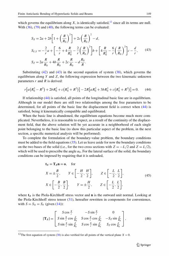
which governs the equilibrium along X, is identically satisfied,12 since all its terms are null.With (36), (79) and (40), the following terms can be evaluated:

SX = 2a + 2b

[1 +

(R

R0

)2]+ 2c

(R

R0

)2

− d,

SY,Y = −2

ra +

[−6

r+ 4

R

R20

− 2

r

(R

R0

)2]b +

[4

R

R20

− 6

r

(R

R0

)2]c − d

r,

SZ = 2aR

R0+ 4b

R

R0+ 2c

R

R0− d

R0

R.

(43)

Substituting (42) and (43) in the second equation of system (38), which governs theequilibrium along Y and Z, the following expression between the two kinematic unknownparameters r and R is derived:

r[a(R2

0 − R2) + 2bR2

0 + c(R2

0 + R2)] − 2R

[aR2

0 + 3bR20 + c

(R2

0 + R2)] = 0. (44)

If relationship (44) is satisfied, all points of the longitudinal basic line are in equilibrium.Although in our model there are still two relationships among the free parameters to bedetermined, for all points of the basic line the displacement field is correct when (44) issatisfied, being it kinematically compatible and equilibrated.

When the basic line is abandoned, the equilibrium equations become much more com-plicated. Nevertheless, it is reasonable to expect, as a result of the continuity of the displace-ment field, that the above solution will be yet accurate in a neighborhood of each singlepoint belonging to the basic line (to show this particular aspect of the problem, in the nextsection, a specific numerical analysis will be performed).

To complete the formulation of the boundary-value problem, the boundary conditionsmust be added to the field equations (35). Let us leave aside for now the boundary conditionson the two bases of the solid (i.e., for the two cross sections with Z = −L/2 and Z = L/2),which will be used to prescribe the angle α0. For the lateral surface of the solid, the boundaryconditions can be imposed by requiring that it is unloaded,

tR = TRn = o, for

X = ±B

2, Y ∈

[−H

2,H

2

], Z ∈

[−L

2,L

2

],

X ∈[−B

2,B

2

], Y = ±H

2, Z ∈

[−L

2,L

2

],

(45)

where tR is the Piola-Kirchhoff stress vector and n is the outward unit normal. Looking atthe Piola-Kirchhoff stress tensor (31), hereafter rewritten in components for convenience,with S = SX = SY (given (14)):

[TR] =⎡⎢⎣

S cos Xr

−S sin Xr

0

S sin Xr

cos ZR0

S cos Xr

cos ZR0

−SZ sin ZR0

S sin Xr

sin ZR0

S cos Xr

sin ZR0

SZ cos ZR0

⎤⎥⎦ , (46)

12The first equation of system (38) is also verified for all points of the vertical plane X = 0.


it can be observed that: (i) to write the conditions (45) only the first two columns are used;(ii) the first two components TR11 and TR12 do not depend on the variable Z; (iii) againindependently from Z, the components TR21 and TR22 , as well as the components TR31 andTR32, vanish when the terms S sin X

rand S cos X

rare zero, respectively. Previous observations

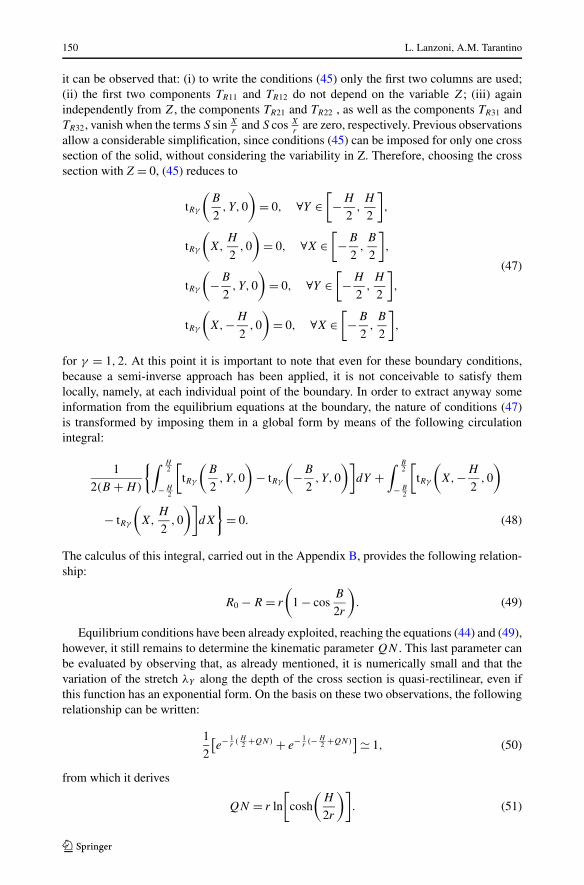
allow a considerable simplification, since conditions (45) can be imposed for only one crosssection of the solid, without considering the variability in Z. Therefore, choosing the crosssection with Z = 0, (45) reduces to

tRγ

(B

2, Y,0

)= 0, ∀Y ∈

[−H

2,H

2

],

tRγ

(X,

H

2,0

)= 0, ∀X ∈

[−B

2,B

2

],

tRγ

(−B

2, Y,0

)= 0, ∀Y ∈

[−H

2,H

2

],

tRγ

(X,−H

2,0

)= 0, ∀X ∈

[−B

2,B

2

],

(47)

for γ = 1,2. At this point it is important to note that even for these boundary conditions,because a semi-inverse approach has been applied, it is not conceivable to satisfy themlocally, namely, at each individual point of the boundary. In order to extract anyway someinformation from the equilibrium equations at the boundary, the nature of conditions (47)is transformed by imposing them in a global form by means of the following circulationintegral:

1

2(B + H)

{∫ H2

− H2

[tRγ

(B

2, Y,0

)− tRγ

(−B

2, Y,0

)]dY +

∫ B2

− B2

[tRγ

(X,−H

2,0

)

− tRγ

(X,

H

2,0

)]dX

}= 0. (48)

The calculus of this integral, carried out in the Appendix B, provides the following relation-ship:

R0 − R = r

(1 − cos

B

2r

). (49)

Equilibrium conditions have been already exploited, reaching the equations (44) and (49),however, it still remains to determine the kinematic parameter QN . This last parameter canbe evaluated by observing that, as already mentioned, it is numerically small and that thevariation of the stretch λY along the depth of the cross section is quasi-rectilinear, even ifthis function has an exponential form. On the basis on these two observations, the followingrelationship can be written:

1

2

[e− 1

r ( H2 +QN) + e− 1

r (− H2 +QN)

] 1, (50)

from which it derives

QN = r ln

[cosh

(H

2r

)]. (51)


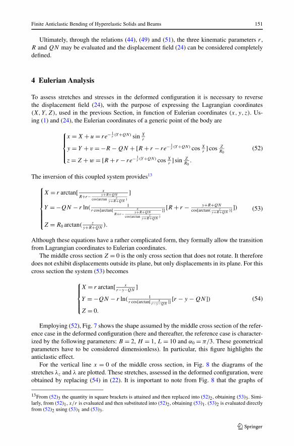
Ultimately, through the relations (44), (49) and (51), the three kinematic parameters r ,R and QN may be evaluated and the displacement field (24) can be considered completelydefined.

4 Eulerian Analysis

To assess stretches and stresses in the deformed configuration it is necessary to reversethe displacement field (24), with the purpose of expressing the Lagrangian coordinates(X,Y,Z), used in the previous Section, in function of Eulerian coordinates (x, y, z). Us-ing (1) and (24), the Eulerian coordinates of a generic point of the body are

⎧⎪⎪⎨⎪⎪⎩

x = X + u = re− 1r (Y+QN) sin X

r

y = Y + v = −R − QN + [R + r − re− 1r (Y+QN) cos X

r] cos Z

R0

z = Z + w = [R + r − re− 1r (Y+QN) cos X

r] sin Z

R0.

(52)

The inversion of this coupled system provides13

⎧⎪⎪⎪⎪⎪⎨⎪⎪⎪⎪⎪⎩

X = r arctan[ x

R+r− y+R+QN

cos(arctan zy+R+QN

)

]

Y = −QN − r ln( 1r cos{arctan[ x

R+r− y+R+QN

cos(arctan zy+R+QN

)

]} [R + r − y+R+QN

cos[arctan( zy+R+QN

)] ])

Z = R0 arctan( zy+R+QN

).

(53)

Although these equations have a rather complicated form, they formally allow the transitionfrom Lagrangian coordinates to Eulerian coordinates.

The middle cross section Z = 0 is the only cross section that does not rotate. It thereforedoes not exhibit displacements outside its plane, but only displacements in its plane. For thiscross section the system (53) becomes

⎧⎪⎪⎨⎪⎪⎩

X = r arctan[ xr−y−QN

]Y = −QN − r ln( 1

r cos{arctan[ xr−y−QN

]} [r − y − QN ])Z = 0.

(54)

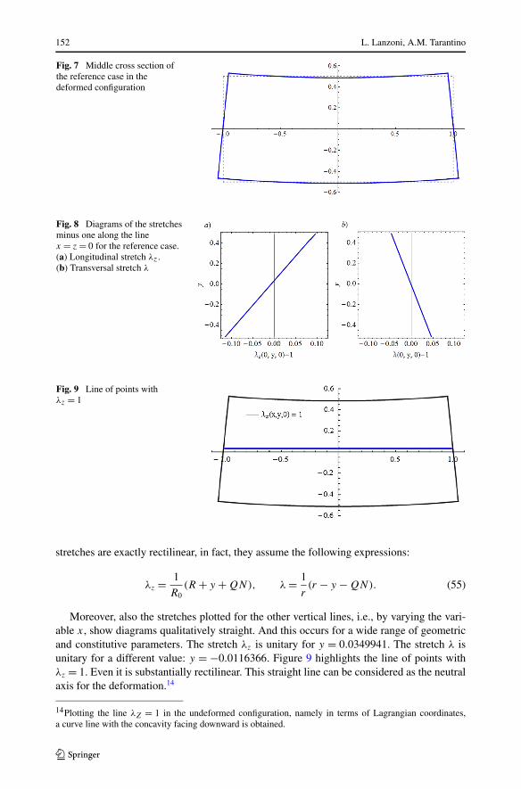
Employing (52), Fig. 7 shows the shape assumed by the middle cross section of the refer-ence case in the deformed configuration (here and thereafter, the reference case is character-ized by the following parameters: B = 2, H = 1, L = 10 and α0 = π/3. These geometricalparameters have to be considered dimensionless). In particular, this figure highlights theanticlastic effect.

For the vertical line x = 0 of the middle cross section, in Fig. 8 the diagrams of thestretches λz and λ are plotted. These stretches, assessed in the deformed configuration, wereobtained by replacing (54) in (22). It is important to note from Fig. 8 that the graphs of

13From (52)3 the quantity in square brackets is attained and then replaced into (52)2, obtaining (53)3. Simi-larly, from (52)1, x/r is evaluated and then substituted into (52)2, obtaining (53)1. (53)2 is evaluated directlyfrom (52)2 using (53)1 and (53)3.


Fig. 7 Middle cross section ofthe reference case in thedeformed configuration

Fig. 8 Diagrams of the stretchesminus one along the linex = z = 0 for the reference case.(a) Longitudinal stretch λz .(b) Transversal stretch λ

Fig. 9 Line of points withλz = 1

stretches are exactly rectilinear, in fact, they assume the following expressions:

λz = 1

R0(R + y + QN), λ = 1

r(r − y − QN). (55)

Moreover, also the stretches plotted for the other vertical lines, i.e., by varying the vari-able x, show diagrams qualitatively straight. And this occurs for a wide range of geometricand constitutive parameters. The stretch λz is unitary for y = 0.0349941. The stretch λ isunitary for a different value: y = −0.0116366. Figure 9 highlights the line of points withλz = 1. Even it is substantially rectilinear. This straight line can be considered as the neutralaxis for the deformation.14

14Plotting the line λZ = 1 in the undeformed configuration, namely in terms of Lagrangian coordinates,a curve line with the concavity facing downward is obtained.


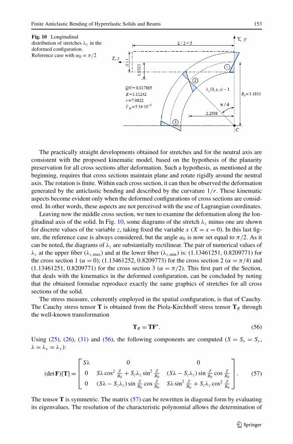
Fig. 10 Longitudinaldistribution of stretches λz in thedeformed configuration.Reference case with α0 = π/2

The practically straight developments obtained for stretches and for the neutral axis areconsistent with the proposed kinematic model, based on the hypothesis of the planaritypreservation for all cross sections after deformation. Such a hypothesis, as mentioned at thebeginning, requires that cross sections maintain plane and rotate rigidly around the neutralaxis. The rotation is finite. Within each cross section, it can then be observed the deformationgenerated by the anticlastic bending and described by the curvature 1/r . These kinematicaspects become evident only when the deformed configurations of cross sections are consid-ered. In other words, these aspects are not perceived with the use of Lagrangian coordinates.

Leaving now the middle cross section, we turn to examine the deformation along the lon-gitudinal axis of the solid. In Fig. 10, some diagrams of the stretch λz minus one are shownfor discrete values of the variable z, taking fixed the variable x (X = x = 0). In this last fig-ure, the reference case is always considered, but the angle α0 is now set equal to π/2. As itcan be noted, the diagrams of λz are substantially rectilinear. The pair of numerical values ofλz at the upper fiber (λz,max) and at the lower fiber (λz,min) is: (1.13461251, 0.8209771) forthe cross section 1 (α = 0); (1.13461252, 0.8209773) for the cross section 2 (α = π/4) and(1.13461251, 0.8209771) for the cross section 3 (α = π/2). This first part of the Section,that deals with the kinematics in the deformed configuration, can be concluded by notingthat the obtained formulae reproduce exactly the same graphics of stretches for all crosssections of the solid.

The stress measure, coherently employed in the spatial configuration, is that of Cauchy.The Cauchy stress tensor T is obtained from the Piola-Kirchhoff stress tensor TR throughthe well-known transformation

TR = TF�. (56)

Using (25), (26), (31) and (56), the following components are computed (S = Sx = Sy ,λ = λx = λy ):

(det F)[T] =

⎡⎢⎢⎣

Sλ 0 0

0 Sλ cos2 ZR0

+ Szλz sin2 ZR0

(Sλ − Szλz) sin ZR0

cos ZR0

0 (Sλ − Szλz) sin ZR0

cos ZR0

Sλ sin2 ZR0

+ Szλz cos2 ZR0

⎤⎥⎥⎦ . (57)

The tensor T is symmetric. The matrix (57) can be rewritten in diagonal form by evaluatingits eigenvalues. The resolution of the characteristic polynomial allows the determination of


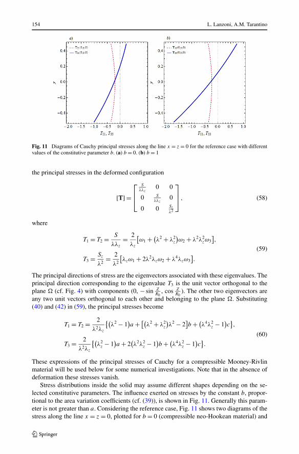
Fig. 11 Diagrams of Cauchy principal stresses along the line x = z = 0 for the reference case with differentvalues of the constitutive parameter b. (a) b = 0. (b) b = 1

the principal stresses in the deformed configuration

[T] =⎡⎢⎣

Sλλz

0 0

0 Sλλz

0

0 0 Sz

λ2

⎤⎥⎦ , (58)

where

T1 = T2 = S

λλz

= 2

λz

[ω1 + (

λ2 + λ2z

)ω2 + λ2λ2

zω3],

T3 = Sz

λ2= 2

λ2

[λzω1 + 2λ2λzω2 + λ4λzω3

].

(59)

The principal directions of stress are the eigenvectors associated with these eigenvalues. Theprincipal direction corresponding to the eigenvalue T3 is the unit vector orthogonal to theplane � (cf. Fig. 4) with components (0, − sin Z

R0, cos Z

R0). The other two eigenvectors are

any two unit vectors orthogonal to each other and belonging to the plane �. Substituting(40) and (42) in (59), the principal stresses become

T1 = T2 = 2

λ2λz

{(λ2 − 1

)a + [(

λ2 + λ2z

)λ2 − 2

]b + (

λ4λ2z − 1

)c},

T3 = 2

λ2λz

{(λ2

z − 1)a + 2

(λ2λ2

z − 1)b + (

λ4λ2z − 1

)c}.

(60)

These expressions of the principal stresses of Cauchy for a compressible Mooney-Rivlinmaterial will be used below for some numerical investigations. Note that in the absence ofdeformation these stresses vanish.

Stress distributions inside the solid may assume different shapes depending on the se-lected constitutive parameters. The influence exerted on stresses by the constant b, propor-tional to the area variation coefficients (cf. (39)), is shown in Fig. 11. Generally this param-eter is not greater than a. Considering the reference case, Fig. 11 shows two diagrams of thestress along the line x = z = 0, plotted for b = 0 (compressible neo-Hookean material) and


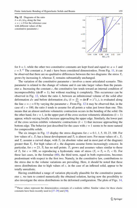
Fig. 12 Diagrams of the ratioδ = dv/dv0 along the linex = z = 0 for the reference casewith different values of theconstitutive parameter c

for b = 1, while the other two constitutive constants are kept fixed and equal to: a = 1 andc = 5.15 The constant a, b and c have been considered dimensionless. From Fig. 11, it canbe observed that there are no qualitative differences between the two diagrams: the stress T3

grows by increasing b, whereas T1 remains substantially unchanged.The variation of the constitutive parameter c involves a more articulated scenario. This

parameter is related to the change of volume and it can take larger values than the param-eter a. Increasing the constant c, the constitutive law tends toward an internal condition ofincompressibility (det F = 1), but without reaching it completely. This occurrence can beobserved in Fig. 12, where the ratio δ, between an infinitesimal volume of the solid afterdeformation dv and before deformation dv0 (δ = dv

dv0= det F = λ2λz), is evaluated along

the line x = z = 0 by varying the parameter c. From Fig. 12 it may be observed that, in thecase of c = 100, the ratio δ tends to assume for all points a value just lower than one. Thismeans that an almost uniform volumetric contraction occurs in the bending of the solid. Onthe other hand, for c = 1, in the upper part of the cross section volumetric dilatations (δ > 1)appear, which varying locally increase approaching the upper edge. Similarly, the lower partof the cross section exhibits volumetric contractions (δ < 1) that increase approaching thebottom edge. The behavior just described for the cases with c = 1 seems to be more naturalfor compressible solids.

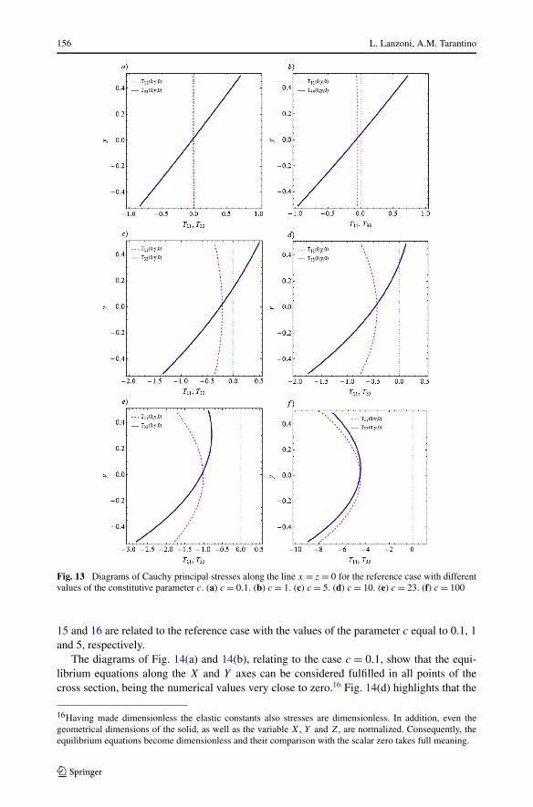
The six images in Fig. 13 display the stress diagrams for c = 0.1,1,5,10,23,100. Forlow values of c, T3 has a linear development and T1 is almost zero. For mean values of c, T3

and T1 assume a curved shape, with T3 (in absolute value and in most part of the diagram)greater than T1. For high values of c, the diagrams assume forms increasingly concave. Inparticular, for c = 23, T3 has no null points. T1 grows and assumes values similar to thoseof T3 for c = 100, so reproducing a hydrostatic state of stress (T1 = T2 = T3 < 0). Forthese last cases, in the formulae (60), the third term, equal in both expressions, becomespredominant with respect to the first two. Namely, in the constitutive law, contributions tothe stress due to the volume variations are prevailing. Here, it should be noted that thesestress distributions due to high values of c, in the case of an inflexed solid, appear to betotally unrealistic.

Having established a range of variation physically plausible for the constitutive param-eter c, we turn to control numerically the obtained solution, having now the possibility toalso investigate the stress distributions in the deformed configuration. The plots of Figs. 14,

15These values represent the dimensionless constants of a realistic rubber. Similar values for these elasticconstants have been recently used in [27–29] and [30].


Fig. 13 Diagrams of Cauchy principal stresses along the line x = z = 0 for the reference case with differentvalues of the constitutive parameter c. (a) c = 0.1. (b) c = 1. (c) c = 5. (d) c = 10. (e) c = 23. (f) c = 100

15 and 16 are related to the reference case with the values of the parameter c equal to 0.1, 1and 5, respectively.

The diagrams of Fig. 14(a) and 14(b), relating to the case c = 0.1, show that the equi-librium equations along the X and Y axes can be considered fulfilled in all points of thecross section, being the numerical values very close to zero.16 Fig. 14(d) highlights that the

16Having made dimensionless the elastic constants also stresses are dimensionless. In addition, even thegeometrical dimensions of the solid, as well as the variable X, Y and Z, are normalized. Consequently, theequilibrium equations become dimensionless and their comparison with the scalar zero takes full meaning.


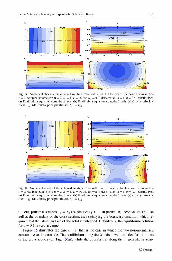
Fig. 14 Numerical check of the obtained solution. Case with c = 0.1. Plots for the deformed cross sectionz = 0. Adopted parameters: B = 2,H = 1, L = 10 and α0 = π/3 (kinematic); a = 1, b = 0.5 (constitutive).(a) Equilibrium equation along the X axis. (b) Equilibrium equation along the Y axis. (c) Cauchy principalstress T33. (d) Cauchy principal stresses T11 = T22

Fig. 15 Numerical check of the obtained solution. Case with c = 1. Plots for the deformed cross sectionz = 0. Adopted parameters: B = 2,H = 1, L = 10 and α0 = π/3 (kinematic); a = 1, b = 0.5 (constitutive).(a) Equilibrium equation along the X axis. (b) Equilibrium equation along the Y axis. (c) Cauchy principalstress T33. (d) Cauchy principal stresses T11 = T22

Cauchy principal stresses T1 = T2 are practically null. In particular, these values are alsonull at the boundary of the cross section, thus satisfying the boundary condition which re-quires that the lateral surface of the solid is unloaded. Definitively, the equilibrium solutionfor c = 0.1 is very accurate.

Figure 15 illustrates the case c = 1, that is the case in which the two non-normalizedconstants a and c coincide. The equilibrium along the X axis is well satisfied for all pointsof the cross section (cf. Fig. 15(a)), while the equilibrium along the Y axis shows some


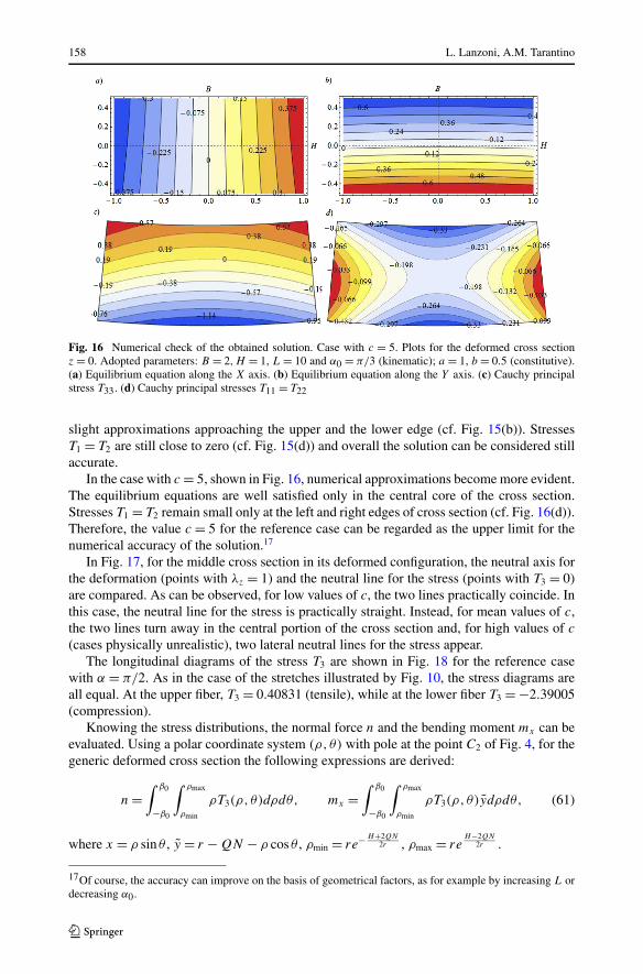
Fig. 16 Numerical check of the obtained solution. Case with c = 5. Plots for the deformed cross sectionz = 0. Adopted parameters: B = 2,H = 1, L = 10 and α0 = π/3 (kinematic); a = 1, b = 0.5 (constitutive).(a) Equilibrium equation along the X axis. (b) Equilibrium equation along the Y axis. (c) Cauchy principalstress T33. (d) Cauchy principal stresses T11 = T22

slight approximations approaching the upper and the lower edge (cf. Fig. 15(b)). StressesT1 = T2 are still close to zero (cf. Fig. 15(d)) and overall the solution can be considered stillaccurate.

In the case with c = 5, shown in Fig. 16, numerical approximations become more evident.The equilibrium equations are well satisfied only in the central core of the cross section.Stresses T1 = T2 remain small only at the left and right edges of cross section (cf. Fig. 16(d)).Therefore, the value c = 5 for the reference case can be regarded as the upper limit for thenumerical accuracy of the solution.17

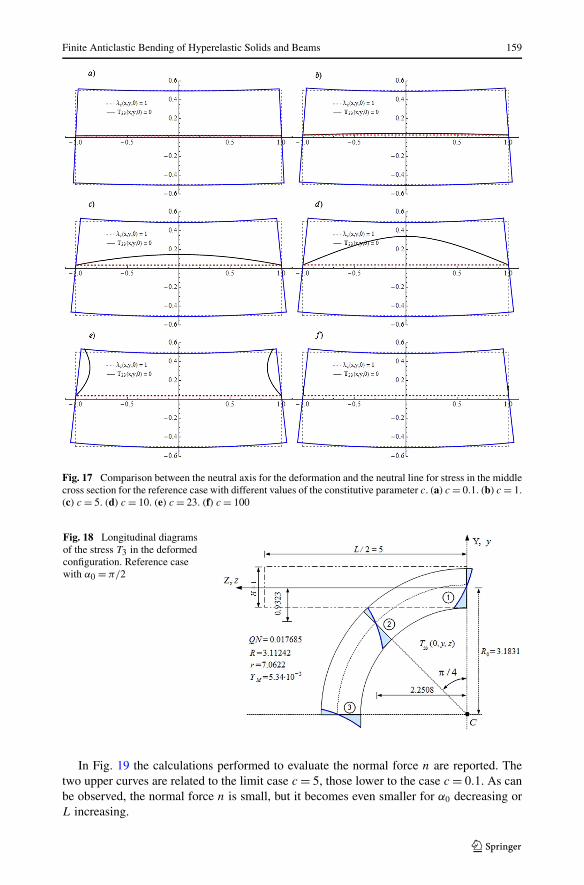
In Fig. 17, for the middle cross section in its deformed configuration, the neutral axis forthe deformation (points with λz = 1) and the neutral line for the stress (points with T3 = 0)are compared. As can be observed, for low values of c, the two lines practically coincide. Inthis case, the neutral line for the stress is practically straight. Instead, for mean values of c,the two lines turn away in the central portion of the cross section and, for high values of c

(cases physically unrealistic), two lateral neutral lines for the stress appear.The longitudinal diagrams of the stress T3 are shown in Fig. 18 for the reference case

with α = π/2. As in the case of the stretches illustrated by Fig. 10, the stress diagrams areall equal. At the upper fiber, T3 = 0.40831 (tensile), while at the lower fiber T3 = −2.39005(compression).

Knowing the stress distributions, the normal force n and the bending moment mx can beevaluated. Using a polar coordinate system (ρ, θ) with pole at the point C2 of Fig. 4, for thegeneric deformed cross section the following expressions are derived:

n =∫ β0

−β0

∫ ρmax

ρmin

ρT3(ρ, θ)dρdθ, mx =∫ β0

−β0

∫ ρmax

ρmin

ρT3(ρ, θ)ydρdθ, (61)

where x = ρ sin θ , y = r − QN − ρ cos θ , ρmin = re− H+2QN2r , ρmax = re

H−2QN2r .

17Of course, the accuracy can improve on the basis of geometrical factors, as for example by increasing L ordecreasing α0.


Fig. 17 Comparison between the neutral axis for the deformation and the neutral line for stress in the middlecross section for the reference case with different values of the constitutive parameter c. (a) c = 0.1. (b) c = 1.(c) c = 5. (d) c = 10. (e) c = 23. (f) c = 100

Fig. 18 Longitudinal diagramsof the stress T3 in the deformedconfiguration. Reference casewith α0 = π/2

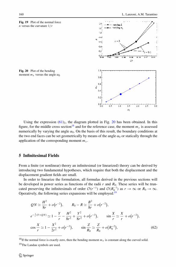
In Fig. 19 the calculations performed to evaluate the normal force n are reported. Thetwo upper curves are related to the limit case c = 5, those lower to the case c = 0.1. As canbe observed, the normal force n is small, but it becomes even smaller for α0 decreasing orL increasing.


Fig. 19 Plot of the normal forcen versus the curvature 1/r

Fig. 20 Plot of the bendingmoment mx versus the angle α0

Using the expression (61)2, the diagram plotted in Fig. 20 has been obtained. In thisfigure, for the middle cross section18 and for the reference case, the moment mx is assessednumerically by varying the angle α0. On the basis of this result, the boundary conditions atthe two end faces can be set geometrically by means of the angle α0 or statically through theapplication of the corresponding moment mx .

5 Infinitesimal Fields

From a finite (or nonlinear) theory an infinitesimal (or linearized) theory can be derived byintroducing two fundamental hypotheses, which require that both the displacement and thedisplacement gradient fields are small.

In order to linearize the formulation, all formulas derived in the previous sections willbe developed in power series as functions of the radii r and R0. These series will be trun-cated preserving the infinitesimals of order O(r−1) and O(R−1

0 ) as r → ∞ or R0 → ∞.Operatively, the following series expansions will be employed:19

QN H 2

8r+ o

(r−2

), R0 − R B2

8r+ o

(r−2

),

e− 1r (Y+QN) 1 − Y

r− H 2

8r2+ Y 2

8r2+ o

(r−3

), sin

X

r X

r+ o

(r−2

),

cosX

r 1 − X2

2r2+ o

(r−3

), sin

Z

R0 Z

R0+ o

(R−2

0

), (62)

18If the normal force is exactly zero, then the bending moment mx is constant along the curved solid.19The Landau symbols are used.


cosZ

R0 1 − Z2

2R20

+ o(R−3

0

), R sin

Z

R0 Z − ZB2

8rR0− Z3

6R20

+ o(R−2

0

),

R cosZ

R0 R − Z2

2R0+ o

(R−2

0

), sinh

H

2r H

2r+ o

(r−2

).

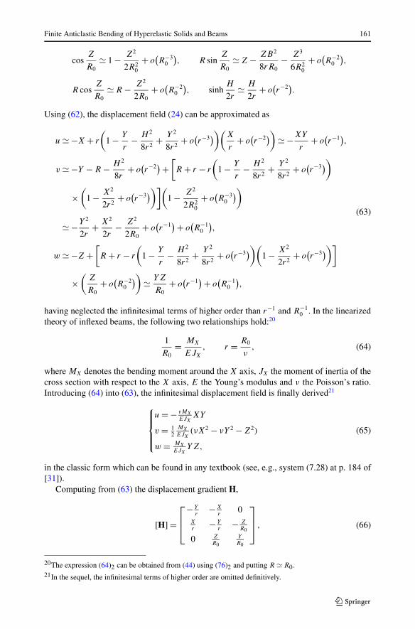
Using (62), the displacement field (24) can be approximated as

u −X + r

(1 − Y

r− H 2

8r2+ Y 2

8r2+ o

(r−3

))(X

r+ o

(r−2

)) −XY

r+ o

(r−1

),

v −Y − R − H 2

8r+ o

(r−2

) +[R + r − r

(1 − Y

r− H 2

8r2+ Y 2

8r2+ o

(r−3

))

×(

1 − X2

2r2+ o

(r−3

))](1 − Z2

2R20

+ o(R−3

0

))

−Y 2

2r+ X2

2r− Z2

2R0+ o

(r−1

) + o(R−1

0

),

w −Z +[R + r − r

(1 − Y

r− H 2

8r2+ Y 2

8r2+ o

(r−3

))(1 − X2

2r2+ o

(r−3

))]

×(

Z

R0+ o

(R−2

0

)) YZ

R0+ o

(r−1

) + o(R−1

0

),

(63)

having neglected the infinitesimal terms of higher order than r−1 and R−10 . In the linearized

theory of inflexed beams, the following two relationships hold:20

1

R0= MX

EJX

, r = R0

ν, (64)

where MX denotes the bending moment around the X axis, JX the moment of inertia of thecross section with respect to the X axis, E the Young’s modulus and ν the Poisson’s ratio.Introducing (64) into (63), the infinitesimal displacement field is finally derived21

⎧⎪⎪⎨⎪⎪⎩

u = − νMX

EJXXY

v = 12

MX

EJX(νX2 − νY 2 − Z2)

w = MX

EJXYZ,

(65)

in the classic form which can be found in any textbook (see, e.g., system (7.28) at p. 184 of[31]).

Computing from (63) the displacement gradient H,

[H] =⎡⎢⎣

− Yr

−Xr

0Xr

− Yr

− ZR0

0 ZR0

YR0

⎤⎥⎦ , (66)

20The expression (64)2 can be obtained from (44) using (76)2 and putting R R0.21In the sequel, the infinitesimal terms of higher order are omitted definitively.


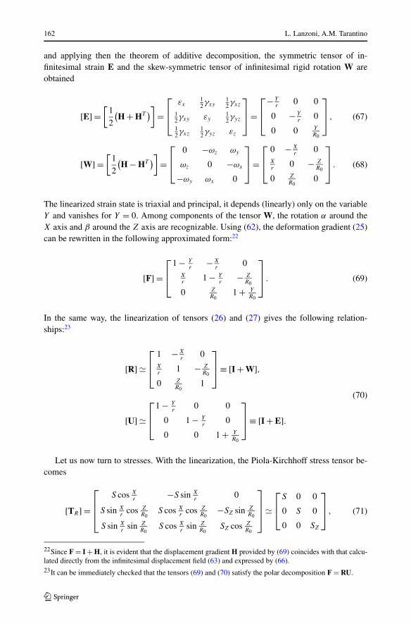
and applying then the theorem of additive decomposition, the symmetric tensor of in-finitesimal strain E and the skew-symmetric tensor of infinitesimal rigid rotation W areobtained

[E] =[

1

2

(H + HT

)] =⎡⎢⎣

εx12γxy

12γxz

12 γxy εy

12γyz

12γxz

12γyz εz

⎤⎥⎦ =

⎡⎢⎣

− Yr

0 0

0 − Yr

0

0 0 YR0

⎤⎥⎦ , (67)

[W] =[

1

2

(H − HT

)] =⎡⎢⎣

0 −ωz ωy

ωz 0 −ωx

−ωy ωx 0

⎤⎥⎦ =

⎡⎢⎣

0 −Xr

0Xr

0 − ZR0

0 ZR0

0

⎤⎥⎦ . (68)

The linearized strain state is triaxial and principal, it depends (linearly) only on the variableY and vanishes for Y = 0. Among components of the tensor W, the rotation α around theX axis and β around the Z axis are recognizable. Using (62), the deformation gradient (25)can be rewritten in the following approximated form:22

[F] =⎡⎢⎣

1 − Yr

−Xr

0Xr

1 − Yr

− ZR0

0 ZR0

1 + YR0

⎤⎥⎦ . (69)

In the same way, the linearization of tensors (26) and (27) gives the following relation-ships:23

[R] ⎡⎢⎣

1 −Xr

0Xr

1 − ZR0

0 ZR0

1

⎤⎥⎦ ≡ [I + W],

[U] ⎡⎢⎣

1 − Yr

0 0

0 1 − Yr

0

0 0 1 + YR0

⎤⎥⎦ ≡ [I + E].

(70)

Let us now turn to stresses. With the linearization, the Piola-Kirchhoff stress tensor be-comes

[TR] =

⎡⎢⎢⎣

S cos Xr

−S sin Xr

0

S sin Xr

cos ZR0

S cos Xr

cos ZR0

−SZ sin ZR0

S sin Xr

sin ZR0

S cos Xr

sin ZR0

SZ cos ZR0

⎤⎥⎥⎦

⎡⎢⎣

S 0 0

0 S 0

0 0 SZ

⎤⎥⎦ , (71)

22Since F = I + H, it is evident that the displacement gradient H provided by (69) coincides with that calcu-lated directly from the infinitesimal displacement field (63) and expressed by (66).23It can be immediately checked that the tensors (69) and (70) satisfy the polar decomposition F = RU.


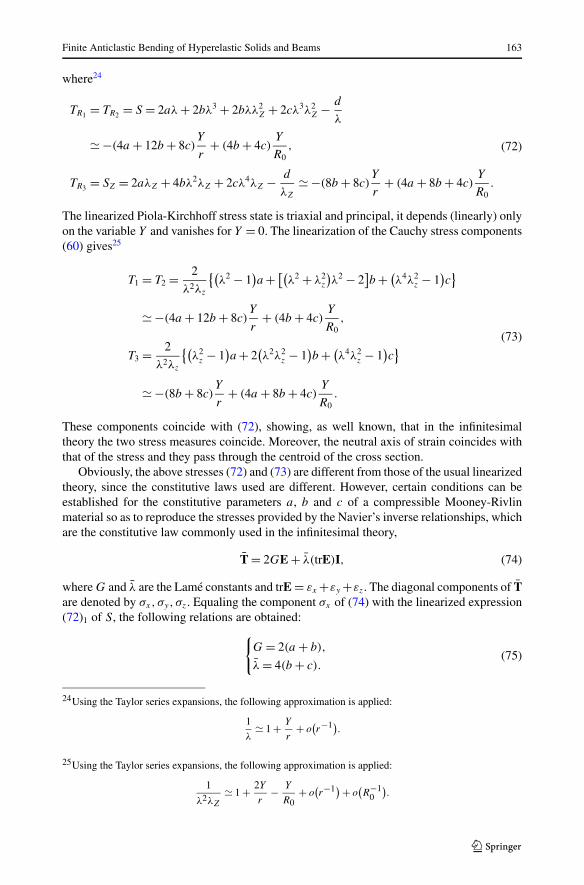
where24

TR1 = TR2 = S = 2aλ + 2bλ3 + 2bλλ2Z + 2cλ3λ2

Z − d

λ

−(4a + 12b + 8c)Y

r+ (4b + 4c)

Y

R0,

TR3 = SZ = 2aλZ + 4bλ2λZ + 2cλ4λZ − d

λZ

−(8b + 8c)Y

r+ (4a + 8b + 4c)

Y

R0.

(72)

The linearized Piola-Kirchhoff stress state is triaxial and principal, it depends (linearly) onlyon the variable Y and vanishes for Y = 0. The linearization of the Cauchy stress components(60) gives25

T1 = T2 = 2

λ2λz

{(λ2 − 1

)a + [(

λ2 + λ2z

)λ2 − 2

]b + (

λ4λ2z − 1

)c}

−(4a + 12b + 8c)Y

r+ (4b + 4c)

Y

R0,

T3 = 2

λ2λz

{(λ2

z − 1)a + 2

(λ2λ2

z − 1)b + (

λ4λ2z − 1

)c}

−(8b + 8c)Y

r+ (4a + 8b + 4c)

Y

R0.

(73)

These components coincide with (72), showing, as well known, that in the infinitesimaltheory the two stress measures coincide. Moreover, the neutral axis of strain coincides withthat of the stress and they pass through the centroid of the cross section.

Obviously, the above stresses (72) and (73) are different from those of the usual linearizedtheory, since the constitutive laws used are different. However, certain conditions can beestablished for the constitutive parameters a, b and c of a compressible Mooney-Rivlinmaterial so as to reproduce the stresses provided by the Navier’s inverse relationships, whichare the constitutive law commonly used in the infinitesimal theory,

T = 2GE + λ(trE)I, (74)

where G and λ are the Lamé constants and trE = εx +εy +εz. The diagonal components of Tare denoted by σx, σy, σz. Equaling the component σx of (74) with the linearized expression(72)1 of S, the following relations are obtained:

{G = 2(a + b),

λ = 4(b + c).(75)

24Using the Taylor series expansions, the following approximation is applied:

1

λ 1 + Y

r+ o

(r−1)

.

25Using the Taylor series expansions, the following approximation is applied:

1

λ2λZ

1 + 2Y

r− Y

R0+ o

(r−1) + o

(R−1

0

).


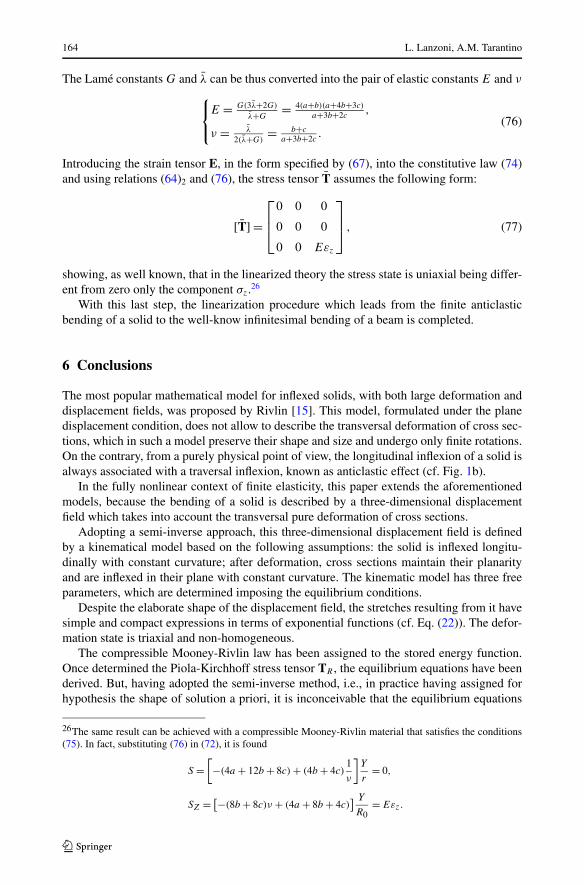
The Lamé constants G and λ can be thus converted into the pair of elastic constants E and ν

⎧⎨⎩

E = G(3λ+2G)

λ+G= 4(a+b)(a+4b+3c)

a+3b+2c,

ν = λ

2(λ+G)= b+c

a+3b+2c.

(76)

Introducing the strain tensor E, in the form specified by (67), into the constitutive law (74)and using relations (64)2 and (76), the stress tensor T assumes the following form:

[T] =⎡⎢⎣

0 0 0

0 0 0

0 0 Eεz

⎤⎥⎦ , (77)

showing, as well known, that in the linearized theory the stress state is uniaxial being differ-ent from zero only the component σz.26

With this last step, the linearization procedure which leads from the finite anticlasticbending of a solid to the well-know infinitesimal bending of a beam is completed.

6 Conclusions

The most popular mathematical model for inflexed solids, with both large deformation anddisplacement fields, was proposed by Rivlin [15]. This model, formulated under the planedisplacement condition, does not allow to describe the transversal deformation of cross sec-tions, which in such a model preserve their shape and size and undergo only finite rotations.On the contrary, from a purely physical point of view, the longitudinal inflexion of a solid isalways associated with a traversal inflexion, known as anticlastic effect (cf. Fig. 1b).

In the fully nonlinear context of finite elasticity, this paper extends the aforementionedmodels, because the bending of a solid is described by a three-dimensional displacementfield which takes into account the transversal pure deformation of cross sections.

Adopting a semi-inverse approach, this three-dimensional displacement field is definedby a kinematical model based on the following assumptions: the solid is inflexed longitu-dinally with constant curvature; after deformation, cross sections maintain their planarityand are inflexed in their plane with constant curvature. The kinematic model has three freeparameters, which are determined imposing the equilibrium conditions.

Despite the elaborate shape of the displacement field, the stretches resulting from it havesimple and compact expressions in terms of exponential functions (cf. Eq. (22)). The defor-mation state is triaxial and non-homogeneous.

The compressible Mooney-Rivlin law has been assigned to the stored energy function.Once determined the Piola-Kirchhoff stress tensor TR , the equilibrium equations have beenderived. But, having adopted the semi-inverse method, i.e., in practice having assigned forhypothesis the shape of solution a priori, it is inconceivable that the equilibrium equations

26The same result can be achieved with a compressible Mooney-Rivlin material that satisfies the conditions(75). In fact, substituting (76) in (72), it is found

S =[−(4a + 12b + 8c) + (4b + 4c)

1

ν

]Y

r= 0,

SZ = [−(8b + 8c)ν + (4a + 8b + 4c)] Y

R0= Eεz.


can be correctly solved for all points of the solid. Nevertheless, a basic longitudinal line hasbeen recognized, where the compatibility and equilibrium conditions are fully satisfied.

To assess the accuracy of the displacement field in correspondence of the other points,the equilibrium equations were normalized and, by means of numerical analyses, it was es-timated how much they deviate from zero as one moves away from the basic line. Through aset of diagrams, the existence of a central core surrounding the basic line, where the solutionproposed can be considered acceptable, has been highlighted. The extension of this centralcore depends on the parameters involved. The most important geometric parameters are thelength of the solid L and the angle of inflexion α0, because the central core becomes wideras L increases and as α0 decreases.

Once completed the Lagrangian analysis, the Eulerian analysis was conducted with thepurpose of evaluating stretches and stresses in the deformed configuration. The expressionsof the Cauchy principal stresses have been obtained (cf. Eq. (60)) and the effective stressdistributions in the inflexed solid are shown by some diagrams. Successively, the influenceexerted on these stresses by the normalized constitutive parameters b and c have been inves-tigated (cf. Figs. 11 and 13).

The parameter b does not exert a qualitative influence on the stress distributions in crosssections. More care is needed for the parameter c. When the parameter c is small or at mostequal to the first constitutive parameter a, the obtained solution is numerically accurate,since the equilibrium equations are well satisfied for all points of the cross sections and thelateral surface of the solid is unloaded (cf. Figs. 14 and 15). Increasing the value of theparameter c, the approximations become more evident. The case c = 5 may be consideredthe upper limit for a numerically accurate solution (cf. Fig. 16).

By varying the parameter c, a comparison was made between the neutral line for thestress (T3 = 0) and the neutral axis for the deformation (λz = 1). For low values of c, thetwo lines coincide. For average values of c, the two lines differ. In particular, the neutral linefor the stress assumes a curved shape. For high values of c (cases physically unrealistic),two distinct neutral lines for the stress even appear (cf. Fig. 17).

Knowing the stress distributions, explicit formulae to calculate the normal force and thebending moment in the deformed configuration were given (cf. Eq. (61)). A further verifi-cation of the obtained solution was made by checking that the normal force is close to zero.Being available the expression for the bending moment, the value of the moment needed toproduce a specific inflexion angle α0 can be assessed. This allows to impose the boundaryconditions statically, through the application on the two end faces of the solid of a pair ofbending moments (cf. Fig. 20).

The whole formulation exposed in the paper for the finite anticlastic bending of hypere-lastic solids was linearized by introducing the hypothesis of smallness of the displacementand strain fields. All derived formulae were rewritten as power series. These series, whichdepend on the radii r and R0, were truncated by preserving the first order infinitesimals asr → ∞ and R0 → ∞.

Operating in this way, the nonlinear displacement field (24) was linearized getting exactlythe well-known displacement field of the linear theory of inflexed beams (cf. Eq. (65)).

Unlike to what was obtained using the finite theory, in the infinitesimal theory the neutralaxis of strain coincides with the neutral line of the stress and they pass through the centroidof the cross section.

The linearization procedure, based on the assumptions of smallness, has shown the tran-sition from the proposed solution for the finite anticlastic bending of solids to the classicalsolution for the infinitesimal bending of beams.


Acknowledgements Authors acknowledge funding from Italian Ministry MIUR-PRIN voce COAN5.50.16.01 code 2015JW9NJT.

Open Access This article is distributed under the terms of the Creative Commons Attribution 4.0 Inter-national License (http://creativecommons.org/licenses/by/4.0/), which permits unrestricted use, distribution,and reproduction in any medium, provided you give appropriate credit to the original author(s) and the source,provide a link to the Creative Commons license, and indicate if changes were made.

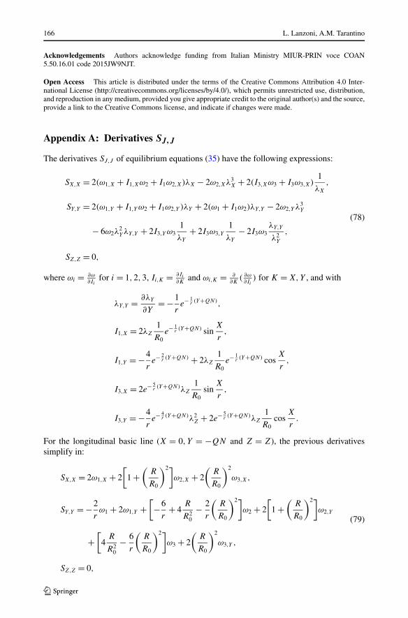
Appendix A: Derivatives SJ,J

The derivatives SJ,J of equilibrium equations (35) have the following expressions:

SX,X = 2(ω1,X + I1,Xω2 + I1ω2,X)λX − 2ω2,Xλ3X + 2(I3,Xω3 + I3ω3,X)

1

λX

,

SY,Y = 2(ω1,Y + I1,Y ω2 + I1ω2,Y )λY + 2(ω1 + I1ω2)λY,Y − 2ω2,Y λ3Y

− 6ω2λ2Y λY,Y + 2I3,Y ω3

1

λY

+ 2I3ω3,Y

1

λY

− 2I3ω3λY,Y

λ2Y

,

SZ,Z = 0,

(78)

where ωi = ∂ω∂Ii

for i = 1,2,3, Ii,K = ∂Ii∂K

and ωi,K = ∂∂K

( ∂ω∂Ii

) for K = X,Y , and with

λY,Y = ∂λY

∂Y= −1

re− 1

r (Y+QN),

I1,X = 2λZ

1

R0e− 1

r (Y+QN) sinX

r,

I1,Y = −4

re− 2

r (Y+QN) + 2λZ

1

R0e− 1

r (Y+QN) cosX

r,

I3,X = 2e− 5r (Y+QN)λZ

1

R0sin

X

r,

I3,Y = −4

re− 4

r (Y+QN)λ2Z + 2e− 5

r (Y+QN)λZ

1

R0cos

X

r.

For the longitudinal basic line (X = 0, Y = −QN and Z = Z), the previous derivativessimplify in:

SX,X = 2ω1,X + 2

[1 +

(R

R0

)2]ω2,X + 2

(R

R0

)2

ω3,X,

SY,Y = −2

rω1 + 2ω1,Y +

[−6

r+ 4

R

R20

− 2

r

(R

R0

)2]ω2 + 2

[1 +

(R

R0

)2]ω2,Y

+[

4R

R20

− 6

r

(R

R0

)2]ω3 + 2

(R

R0

)2

ω3,Y ,

SZ,Z = 0,

(79)


with

I1 = 2 +(

R

R0

)2

, I1,X = 0, I1,Y = −4

r+ 2R

R20

,

I3 =(

R

R0

), I3,X = 0, I3,Y = −4

r

(R

R0

)2

+ 2R

R20

,

SX = 2ω1 + 2ω2 + 2

(R

R0

)2

ω2 + 2

(R

R0

)2

ω3,

SZ = 2ω1R

R0+ 4ω2

R

R0+ 2ω3

R

R0.

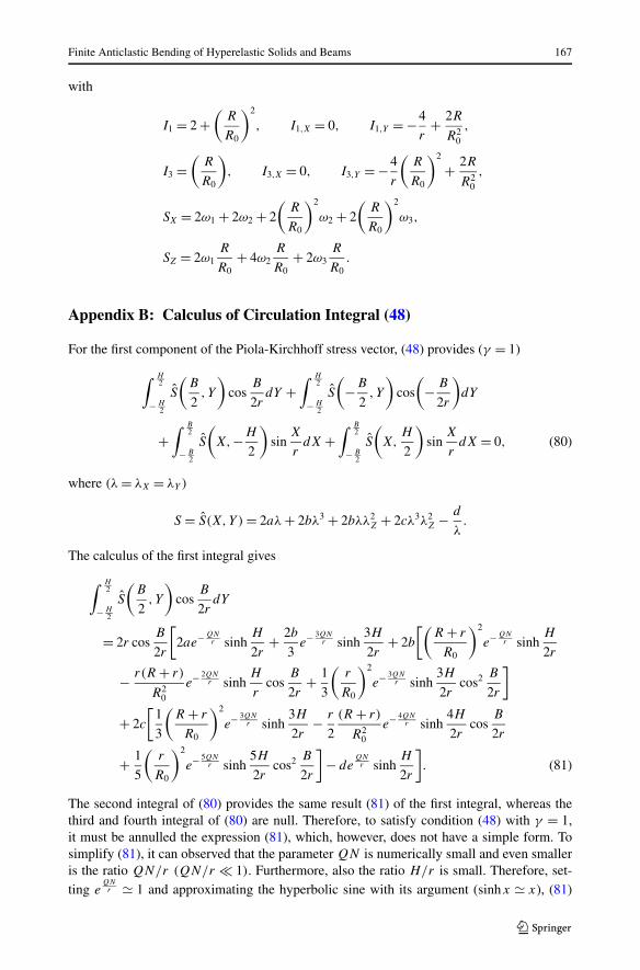
Appendix B: Calculus of Circulation Integral (48)

For the first component of the Piola-Kirchhoff stress vector, (48) provides (γ = 1)

∫ H2

− H2

S

(B

2, Y

)cos

B

2rdY +

∫ H2

− H2

S

(−B

2, Y

)cos

(− B

2r

)dY

+∫ B

2

− B2

S

(X,−H

2

)sin

X

rdX +

∫ B2

− B2

S

(X,

H

2

)sin

X

rdX = 0, (80)

where (λ = λX = λY )

S = S(X,Y ) = 2aλ + 2bλ3 + 2bλλ2Z + 2cλ3λ2

Z − d

λ.

The calculus of the first integral gives

∫ H2

− H2

S

(B

2, Y

)cos

B

2rdY

= 2r cosB

2r

[2ae− QN

r sinhH

2r+ 2b

3e− 3QN

r sinh3H

2r+ 2b

[(R + r

R0

)2

e− QNr sinh

H

2r

− r(R + r)

R20

e− 2QNr sinh

H

rcos

B

2r+ 1

3

(r

R0

)2

e− 3QNr sinh

3H

2rcos2 B

2r

]

+ 2c

[1

3

(R + r

R0

)2

e− 3QNr sinh

3H

2r− r

2

(R + r)

R20

e− 4QNr sinh

4H

2rcos

B

2r

+ 1

5

(r

R0

)2

e− 5QNr sinh

5H

2rcos2 B

2r

]− de

QNr sinh

H

2r

]. (81)

The second integral of (80) provides the same result (81) of the first integral, whereas thethird and fourth integral of (80) are null. Therefore, to satisfy condition (48) with γ = 1,it must be annulled the expression (81), which, however, does not have a simple form. Tosimplify (81), it can observed that the parameter QN is numerically small and even smalleris the ratio QN/r (QN/r � 1). Furthermore, also the ratio H/r is small. Therefore, set-ting e

QNr 1 and approximating the hyperbolic sine with its argument (sinhx x), (81)


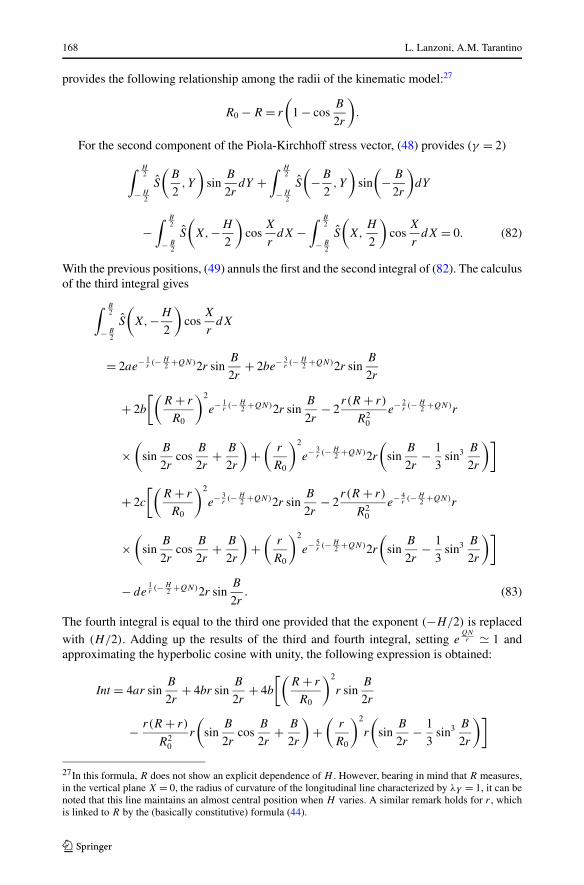
provides the following relationship among the radii of the kinematic model:27

R0 − R = r

(1 − cos

B

2r

).

For the second component of the Piola-Kirchhoff stress vector, (48) provides (γ = 2)

∫ H2

− H2

S

(B

2, Y

)sin

B

2rdY +

∫ H2

− H2

S

(−B

2, Y

)sin

(− B

2r

)dY

−∫ B

2

− B2

S

(X,−H

2

)cos

X

rdX −

∫ B2

− B2

S

(X,

H

2

)cos

X

rdX = 0. (82)

With the previous positions, (49) annuls the first and the second integral of (82). The calculusof the third integral gives

∫ B2

− B2

S

(X,−H

2

)cos

X

rdX

= 2ae− 1r (− H

2 +QN)2r sinB

2r+ 2be− 3

r (− H2 +QN)2r sin

B

2r

+ 2b

[(R + r

R0

)2

e− 1r (− H

2 +QN)2r sinB

2r− 2

r(R + r)

R20

e− 2r (− H

2 +QN)r

×(

sinB

2rcos

B

2r+ B

2r

)+

(r

R0

)2

e− 3r (− H

2 +QN)2r

(sin

B

2r− 1

3sin3 B

2r

)]

+ 2c

[(R + r

R0

)2

e− 3r (− H

2 +QN)2r sinB

2r− 2

r(R + r)

R20

e− 4r (− H

2 +QN)r

×(

sinB

2rcos

B

2r+ B

2r

)+

(r

R0

)2

e− 5r (− H

2 +QN)2r

(sin

B

2r− 1

3sin3 B

2r

)]

− de1r (− H

2 +QN)2r sinB

2r. (83)

The fourth integral is equal to the third one provided that the exponent (−H/2) is replacedwith (H/2). Adding up the results of the third and fourth integral, setting e

QNr 1 and

approximating the hyperbolic cosine with unity, the following expression is obtained:

Int = 4ar sinB

2r+ 4br sin

B

2r+ 4b

[(R + r

R0

)2

r sinB

2r

− r(R + r)

R20

r

(sin

B

2rcos

B

2r+ B

2r

)+

(r

R0

)2

r

(sin

B

2r− 1

3sin3 B

2r

)]

27In this formula, R does not show an explicit dependence of H . However, bearing in mind that R measures,in the vertical plane X = 0, the radius of curvature of the longitudinal line characterized by λY = 1, it can benoted that this line maintains an almost central position when H varies. A similar remark holds for r , whichis linked to R by the (basically constitutive) formula (44).


+ 4c

[(R + r

R0

)2

r sinB

2r− r(R + r)

R20

r

(sin

B

2rcos

B

2r+ B

2r

)

+(

r

R0

)2

r

(sin

B

2r− 1

3sin3 B

2r

)]− 2dr sin

B

2r. (84)

This expression can be rearranged by using expression (49), however it does not completelyvanish but it exhibits some residual terms,

Int = 4(a + b)

(r

R0

)2[(R + r)

(sin

B

2rcos

B

2r− B

2r

)+ 2

3r sin3 B

2r

], (85)

that become numerically negligible as B decreases with respect to r .Essentially with this last remark also the boundary conditions can be considered fulfilled,

of course on average over the whole boundary and with some numerical approximations. Inany case, the procedure followed has allowed to obtain the formula (49), which has a simpleand compact form, despite the complexity of the problem studied.

References

1. Bernoulli, J.: Specimen alterum calculi differentialis in dimetienda spirali logarithmica, loxodromiisnautarum et areis triangulorum sphaericorum. Una cum additamento quodam ad problema funicularium,aliisque. Acta Eruditorum, Junii (1691) 282–290—Opera 442–453

2. Bernoulli, J.: Vritable hypothse de la rsistance des solides, avec la dmonstration de la courbure des corpsqui font ressort. Académie Royale des Sciences, Paris (1705)

3. Parent, A.: Essais et Recherches de Mathmétique et de Physique. Nouv. Ed., Paris (1713)4. Euler, L.: Mechanica, sive, Motus scientia analytice exposita. Petropoli: ex typographia Academiae Sci-

entiarum (1736)5. Euler, L.: Additamentum I de curvis elasticis, methodus inveniendi lineas curvas maximi minimivi pro-

prietate gaudentes. Bousquent, Lausanne (1744)6. Euler, L.: Genuina principia doctrinae de statu aequilibrii et motu corporum tam perfecte flexibilium

quam elasticorum. Opera Omnia II 11, 37–61 (1771)7. Euler, L.: De gemina methodo tam aequilibrium quam motum corporum flexibilium determinandi et

utriusque egregio consensu. Novi Comment. Acad. Sci. Petropol. 20, 286–303 (1776)8. Navier, C.L.M.H.: Mémoire sur les lois de l’équilibre et du mouvement des corps solides élastiques.

Mém. Acad. Sci. Inst. Fr. 7, 375–393 (1821)9. Barr de Saint-Venant, A.-J-C.: Memoire sur la torsion des prismes. C. R. Acad. Sci. 37 (1853)

10. Bresse, J.A.C.: Recherches analytiques sur la flexion et la résistance des pices courbes. Carilian-Goeuryet VrDalmont libraires, Paris (1854)

11. Lamb, H.: Sur la flexion d’un ressort élastique plat. Philos. Mag. 31, 182–188 (1891)12. Thomson (Lord Kelvin), W., Tait, P.G.: Treatise on Natural Philosophy. Cambridge University Press,

Cambridge (1867)13. Love, A.E.H.: A Treatise on the Mathematical Theory of Elasticity, 4th edn. Cambridge University Press,

Cambridge (1927)14. Seth, B.R.: Finite strain in elastic problems. Proc. R. Soc. Lond. A 234, 231–264 (1935)15. Rivlin, R.S.: Large elastic deformations of isotropic materials. V. The problem of flexure. Proc. R. Soc.

Lond. A 195, 463–473 (1949)16. Rivlin, R.S.: Large elastic deformations of isotropic materials. VI. Further results in the theory of torsion,

shear and flexure. Proc. R. Soc. Lond. A 242, 173–195 (1949)17. Shield, R.T.: Bending of a beam or wide strip. Q. J. Mech. Appl. Math. 45, 567–573 (1992)18. Bruhns, O.T., Xiao, H., Meyers, A.: Finite bending of a rectangular block of an elastic Hencky material.

J. Elast. 66, 237–256 (2002)19. Ferguson, A., Andrews, J.P.: An experimental study of the anticlastic bending of rectangular bars of

different cross-section. Proc. Phys. Soc. 41, 1–17 (1928)20. Conway, H.D., Nickola, W.E.: Anticlastic action of flat sheets in bending. Exp. Mech. 5, 115–119 (1965)


21. Tarantino, A.M.: Thin hyperelastic sheets of compressible material: field equations, airy stress functionand an application in fracture mechanics. J. Elast. 44, 37–59 (1996)

22. Tarantino, A.M.: The singular equilibrium field at the notch-tip of a compressible material in finite elas-tostatics. Z. Angew. Math. Phys. 48, 370–388 (1997)

23. Tarantino, A.M.: On extreme thinning at the notch-tip of a neo-Hookean sheet. Q. J. Mech. Appl. Math.51(2), 179–190 (1998)

24. Tarantino, A.M.: On the finite motions generated by a mode I propagating crack. J. Elast. 57, 85–103(1999)

25. Tarantino, A.M.: Crack propagation in finite elastodynamics. Math. Mech. Solids 10, 577–601 (2005)26. Tarantino, A.M.: Nonlinear fracture mechanics for an elastic Bell material. Q. J. Mech. Appl. Math. 50,

435–456 (1997)27. Tarantino, A.M.: Equilibrium paths of a hyperelastic body under progressive damage. J. Elast. 114, 225–

250 (2014)28. Lanzoni, L., Tarantino, A.M.: Damaged hyperelastic membranes. Int. J. Non-Linear Mech. 60, 9–22

(2014)29. Lanzoni, L., Tarantino, A.M.: Equilibrium configurations and stability of a damaged body under uniaxial

tractions. Z. Angew. Math. Phys. 66, 171–190 (2015)30. Lanzoni, L., Tarantino, A.M.: A simple nonlinear model to simulate the localized necking and neck

propagation. Int. J. Non-Linear Mech. 84, 94–104 (2016)31. Tarantino, A.M.: Scienza delle Costruzioni. Pitagora Editrice Bologna, Bologna (2005). In Italian

Documents

Finite Anticlastic Bending of Hyperelastic Solids and · PDF fileFinite Anticlastic Bending of Hyperelastic ... on the strain according to the linearized theory ... Anticlastic Bending