Fast porous visco-hyperelastic soft tissue model for surgery simulation:application to liver surgery

Stephanie Marchesseaua, Tobias Heimanna, Simon Chatelinb, Remy Willingerb, Herve Delingettea

aAsclepios Research Project, INRIA Sophia Antipolis, FrancebUniversity of Strasbourg, IMFS-CNRS, Strasbourg, France

Abstract

Understanding and modeling liver biomechanics represents a significant challenge due to its complex nature. In thispaper, we tackle this issue in the context of real time surgery simulation where a compromise between biomechanicalaccuracy and computational efficiency must be found. We describe a realistic liver model including hyperelasticity,porosity and viscosity that is implemented within an implicit time integration scheme. To optimize its computation, weintroduce the Multiplicative Jacobian Energy Decomposition (MJED) method for discretizing hyperelastic materialson linear tetrahedral meshes which leads to faster matrix assembly than the standard Finite Element Method. Visco-hyperelasticity is modeled by Prony series while the mechanical effect of liver perfusion is represented with a linearDarcy law. Dynamic mechanical analysis has been performed on 60 porcine liver samples in order to identify somevisco-elastic parameters. Finally, we show that liver deformation can be simulated in real-time on a coarse mesh andstudy the relative effects of the hyperelastic, viscous and porous components on the liver biomechanics.

Keywords: hyperelastic, viscous, porous, liver, real-time simulation, MJED.

1. Introduction

The simulation of soft tissue deformation has at-tracted a growing interest in the past 15 years both inthe biomechanics and the medical image analysis com-munities. Indeed, medical image modalities such asMRI, CT or echography can describe with millimeteraccuracy the anatomical shape of soft tissues but alsotheir deformation through time series of images suchas cine-MRI or electrocardiography. Modeling in sil-ico the deformation of soft tissues is of high interest inparticular for the following applications: surgical ges-ture training[1], therapy planning[2], physically-basedimage registration[3] as well as medical imaging diag-nosis.

In this paper, we focus on the simulation of liver de-formation in the context of surgery training. The overallobjective is to build a simulator that can ease the train-ing of young medical residents to perform some ges-tures specific to minimally invasive surgery such as la-paroscopy, endoscopy, interventional radiology, etc. Insuch cases, it is required that soft tissue deformation be

URL: Stephanie.Marchesseau@inria.fr (StephanieMarchesseau)

simulated in real-time, i.e. at nearly 25 frames per sec-ond for the persistence of vision to take place. Obvi-ously with such performance, the simulation algorithmsused in surgical simulators can also be used for surgeryplanning or even computer animation. However, insurgery simulation, there are additional constraints ofnumerical stability during the occurrence of contact be-tween soft tissue and (virtual) surgical instruments. Be-cause those instruments are controlled by a human oper-ator, large compression or extension of tissue can occur,sometimes leading to non-physical behavior such as in-verted elements.

Because soft biological tissue behavior is rather com-plex and also not well characterized, its simulation inreal-time is a very challenging task. The liver, forinstance, is a porous material which typically under-goes large displacements, large deformations and isalso strongly visco-elastic (more details in section 2.2).Early approaches for modeling the soft tissue behaviorassumed a linear elastic behavior[4] discretized on fi-nite elements which naturally leads to solving a linearsystem of equations whose inverse could eventually beprecomputed[5].

Since linear elastic materials are not suited for largedisplacements, several authors in computer animation

Preprint accepted for publication in PBMB September 15, 2010

have proposed corotational elastic models[6, 7] wherelinear elastic stiffness matrices are rotated for each ele-ment. Those corotational models however do not mini-mize a strain energy and therefore are not the discretiza-tion of a continuum formulation. Also, their behavior isvery restricted to material linearity.

To simulate realistic soft tissue deformation, severalauthors have employed hyperelastic materials minimiz-ing a continuum strain energy. For real-time computa-tion, early approaches have been based on St. VenantKirchhoff materials[1] which exhibit a linear stress-strain relationship. Significant speed-up can be obtainedby using reduced basis of deformation[8] or by groupingexpressions on edges, triangles and tetrahedra[9] whendiscretized on linear tetrahedra. Those approaches arehowever limited to this specific material which has thedrawback of not behaving well under compression.

For general hyperelastic materials, authors have re-lied on the Finite Volume Method[10] to simulatesoft-tissue deformation with explicit time integrationschemes. Similarly, Miller et al.[11] have proposedthe Total Lagrangian Explicit Dynamic (TLED) algo-rithm for which elastic forces are based on the referenceconfiguration unlike the Updated Lagrangian methodwidely used in commercial FEM code. This approachhas been combined with Prony series to model visco-elasticity and has been implemented on Graphics Pro-cessing Units (GPU)[12] to reach real-time computa-tions. However the main limitation of this approach isthat it relies on explicit time integration schemes whichgreatly simplifies the update at each time step but re-quires small time steps to keep the computation stableespecially for stiff materials. Furthermore, with explicitschemes it is necessary to iterate multiple times to prop-agate applied forces from a node to the whole mesh.

In this article, we first introduce the MultiplicativeJacobian Energy Decomposition (MJED): a general al-gorithm to implement hyperelastic materials based ontotal Lagrangian FEM with implicit time integrationschemes. An optimized approach to build the stiffnessmatrix is proposed which is used to solve a linear sys-tem of equations at each time step. Our algorithm allowssome matrix precomputations to be performed thanks toa decomposition of the strain energy isolating the deter-minant of the deformation gradient J and the combina-tion of shape vectors with fourth order elasticity tensors.Furthermore, a specific regularization of the stiffnessmatrix allows to cope with highly compressed elements.

A second contribution of this article is to propose arealistic biomechanical model of the liver which com-bines hyperelasticity, viscoelasticity as well as poro-elasticity. The viscoelasticity of our liver model is based

on Prony series whose parameters have been experi-mentally estimated through a dynamic strain sweep test-ing. Furthermore, those parameters have been validatedby reproducing in silico the experiments performed onliver samples. Finally, we take into account the porousmedium of the liver parenchyma through a poro-elasticmodel which computes the fluid pressure and the result-ing applied pressure on the solid phase.

2. Materials and Methods

The goal of this work is to construct a physically-realistic mechanical model of the liver that is suitablefor the simulation of hepatic surgery. As such, themodel should be as accurate as possible, but efficientenough to allow its application in real-time applications.

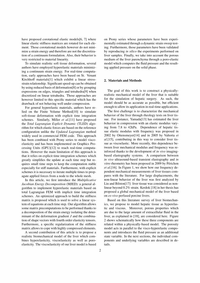
The first challenge is to characterize the mechanicalbehavior of the liver through rheology tests on liver tis-sue. For instance, Yamada[13] has estimated the liverbehavior in compression with an elastic modulus vary-ing from 7.8 to 42kPa. Dependence of hepatic tis-sue elastic modulus with frequency was proposed in2002 by Ottensmeyer[14] and in 2005 by Valtorta etal.[15], contributing in this way to consider liver tis-sue as viscoelastic. More recently, this dependence be-tween liver mechanical modulus and frequency was re-inforced thanks to the development of in vivo imaging-based elastography systems. A comparison betweenin vivo ultrasound-based transient elastography and invitro rheometry has been proposed in 2009 by Perichonet al.[16]. In Figure 1, we show how our frequency de-pendent mechanical measurements of liver tissues com-pares with the literature. For large displacements, thenon-linear behavior of the liver was first analyzed byLiu and Bilston[17]: liver tissue was considered as non-linear beyond 0.2% strain. Kerdok [18] in her thesis hasproposed a global mechanical model of the liver basedon ex-vivo perfused porcine livers.

Based on this literature survey of liver biomechan-ics, we propose to model hepatic tissue as hyperelas-tic and viscous. Moreover, porous properties whichare due to the large amount of extracellular fluid in theliver, as explained in [18], are considered here. Figure2 shows schematically how these three components arerelated within a physically-based model. The porositymodel acts in parallel to the visco-hyperelastic compo-nents and introduces the fluid pressure as an additionalstate variable. In the next sections, the individual com-ponents and underlying variables are described in de-tails.

2

Figure 1: Comparison has been done between classical rheometry (blue), indentation (purple), Magnetic Resonance (red) and Ultrasound-based(green) Elastography tests.

Figure 2: Representation of the constitutive model combining viscos-ity, hyperelasticity and porosity.

2.1. Fast computation of Hyperelastic Materials

Under large deformation, linear elasticity is no longervalid and the liver behavior is better represented as anhyperelastic material. Since we are using implicit timeintegration schemes, it is necessary at each time step tocompute hyperelastic forces and stiffness matrices witha discretization method. The Finite Element Method(FEM) is a widely used approach to this end, howeverthe constraint of real-time simulation is not always sat-

isfied. The objective of this section is to introduce a fastdiscretization method suitable for all hyperelastic mate-rials and to compare it with classical FEM.

To discretize the liver geometry, we use tetrahe-dral linear finite elements because they are straight-forward to generate from triangular surfaces that areoutputted by image segmentation algorithms. Lin-ear tetrahedral finite elements have some limitationssince they can exhibit numerical locking when enforc-ing incompressibility[19]. However, as shown in sec-tion 2.3, the liver is not incompressible at the time scaleconsidered due to the porous nature of the parenchyma.Note also that all optimizations developed in this sec-tion can be easily extended to other elements in partic-ular linear hexahedral elements since it is based on thegradient of shape functions.

In tetrahedral finite elements, TP is the rest tetrahe-dron (with vertices Pi) which is transformed under thedeformation function φ(X) into the tetrahedron TQ (withvertices Qi). Any hyperelastic material is fully deter-mined by its strain energy function Wh which describesthe amount of energy necessary to deform the material.This strain energy function is defined in a way which isinvariant to the application of rigid transformations: itinvolves the invariants of the Cauchy-deformation ten-sor defined as C = ∇φT∇φ. There are numerous invari-ants of C (see [20] for detailed explanation) but the onesused for isotropic materials are the following: I1 = trC,

3

I2 = 12 ((trC)2 − trC2) and the Jacobian J = det∇φ.

We define furthermore the deviatoric deformation ten-sor C = J−2/3C, which by construction does not containany volumetric dilation of the material but only pure de-formation. Its first two invariants are written as I1 andI2.

To capture the resistance to uniform compression orextension, a volumetric energy term U(J) is added, asexplained in section 2.3.

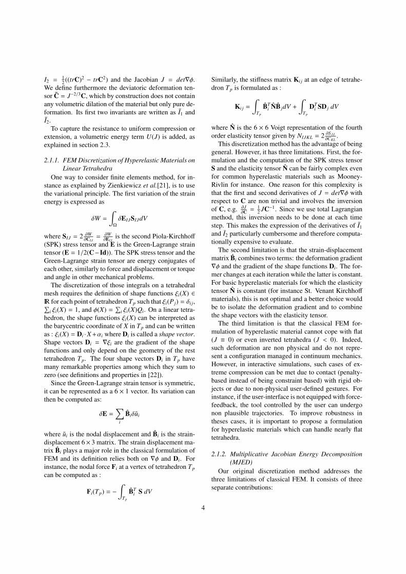
2.1.1. FEM Discretization of Hyperelastic Materials onLinear Tetrahedra

One way to consider finite elements method, for in-stance as explained by Zienkiewicz et al.[21], is to usethe variational principle. The first variation of the strainenergy is expressed as

δW =

∫Ω

δEIJSIJdV

where SIJ = 2 ∂W∂CIJ

= ∂W∂EIJ

is the second Piola-Kirchhoff

(SPK) stress tensor and E is the Green-Lagrange straintensor (E = 1/2(C−Id)). The SPK stress tensor and theGreen-Lagrange strain tensor are energy conjugates ofeach other, similarly to force and displacement or torqueand angle in other mechanical problems.

The discretization of those integrals on a tetrahedralmesh requires the definition of shape functions ξi(X) ∈IR for each point of tetrahedron Tp such that ξi(P j) = δi j,∑

i ξi(X) = 1, and φ(X) =∑

i ξi(X)Qi. On a linear tetra-hedron, the shape functions ξi(X) can be interpreted asthe barycentric coordinate of X in Tp and can be writtenas : ξi(X) = Di ·X +αi where Di is called a shape vector.Shape vectors Di = ∇ξi are the gradient of the shapefunctions and only depend on the geometry of the resttetrahedron Tp. The four shape vectors Di in Tp havemany remarkable properties among which they sum tozero (see definitions and properties in [22]).

Since the Green-Lagrange strain tensor is symmetric,it can be represented as a 6 × 1 vector. Its variation canthen be computed as:

δE =∑

i

Biδui

where ui is the nodal displacement and Bi is the strain-displacement 6× 3 matrix. The strain displacement ma-trix Bi plays a major role in the classical formulation ofFEM and its definition relies both on ∇φ and Di. Forinstance, the nodal force Fi at a vertex of tetrahedron Tp

can be computed as :

Fi(Tp) = −

∫Tp

BTi S dV

Similarly, the stiffness matrix Ki j at an edge of tetrahe-dron Tp is formulated as :

Ki j =

∫Tp

BTi NB jdV +

∫Tp

DTi SD j dV

where N is the 6 × 6 Voigt representation of the fourthorder elasticity tensor given by NIJKL = 2 ∂S IJ

∂CKL.

This discretization method has the advantage of beinggeneral. However, it has three limitations. First, the for-mulation and the computation of the SPK stress tensorS and the elasticity tensor N can be fairly complex evenfor common hyperelastic materials such as Mooney-Rivlin for instance. One reason for this complexity isthat the first and second derivatives of J = det∇φ withrespect to C are non trivial and involves the inversionof C, e.g. ∂J

∂C = 12 JC−1. Since we use total Lagrangian

method, this inversion needs to be done at each timestep. This makes the expression of the derivatives of I1and I2 particularly cumbersome and therefore computa-tionally expensive to evaluate.

The second limitation is that the strain-displacementmatrix Bi combines two terms: the deformation gradient∇φ and the gradient of the shape functions Di. The for-mer changes at each iteration while the latter is constant.For basic hyperelastic materials for which the elasticitytensor N is constant (for instance St. Venant Kirchhoff

materials), this is not optimal and a better choice wouldbe to isolate the deformation gradient and to combinethe shape vectors with the elasticity tensor.

The third limitation is that the classical FEM for-mulation of hyperelastic material cannot cope with flat(J ≡ 0) or even inverted tetrahedra (J < 0). Indeed,such deformation are non physical and do not repre-sent a configuration managed in continuum mechanics.However, in interactive simulations, such cases of ex-treme compression can be met due to contact (penalty-based instead of being constraint based) with rigid ob-jects or due to non-physical user-defined gestures. Forinstance, if the user-interface is not equipped with force-feedback, the tool controlled by the user can undergonon plausible trajectories. To improve robustness intheses cases, it is important to propose a formulationfor hyperelastic materials which can handle nearly flattetrahedra.

2.1.2. Multiplicative Jacobian Energy Decomposition(MJED)

Our original discretization method addresses thethree limitations of classical FEM. It consists of threeseparate contributions:

4

i) Decomposition of strain energyOur approach is to decouple in the strain energy, theinvariants of C from J so as to avoid matrix inver-sions and complex derivative expressions. Instead ofcomputing the force and stiffness matrix using the firstand second derivative of the energy with respect to C(leading respectively to S and N), we compute themdirectly by deriving the energy with respect to the nodalposition:

Fi = −

(∂Wh

∂Qi

)T

and Ki j =

(∂2Wh

∂Q j∂Qi

)(1)

where Wh is the strain energy. It is important to note thatthe approach developed in this section is completelyequivalent to the classical FEM one but leads to moreefficient computation.

We propose to write the strain energy functions asa sum of terms

Wkh = f k(J)gk(I)

or its exponential, where I = (I1, I2, I4...). Thereforegk is independent of J, its derivative will not involveany matrix inversions. This decomposition applies toevery studied case (Veronda Westmann, Arruda-Boyce,St. Venant Kirchhoff, NeoHookean, Ogden, MooneyRivlin and the orthotropic Costa’s law). That gives forinstance

Wh = V0

n∑k=1

f k(J)gk(I)+V0 exp

n′∑k=n+1

f k(J)gk(I)

(2)

Exponential terms here account for models such asCosta’s or Veronda Westmann’s (see [23] for a detaileddescription), the following calculations are made onlyfor non exponential terms.

Using this decomposition of strain energy enablescomplex material formulation to be computed more effi-ciently with only a sum of reasonably simple terms andno matrix inversions. Once the decomposition is done,getting f k′(J) requires a 1D derivation, and getting Sk

h =

2 ∂gk(I)∂C requires to combine well-known derivatives of

the invariants (such as ∂I1∂C = Id or ∂I2

∂C = IdI1 −C whereId is the 3 × 3 identity matrix). The full derivation, ex-plained in Appendix A, gives

Fh,i = −V0

n∑k=1

f k′(J)gk(I)(∂J∂Qi

)T

+ f k(J)∇φ Skh Di

where the derivative of the Jacobian is expressed as

∂J∂Qi

=1

6V0((Q j − Ql) ∧ (Qk − Ql))T

ii) Formulation of the stiffness matrixImplicit time integration schemes require the computa-tion of the tangent stiffness matrix at each time step.This naturally involves elasticity tensors computed asthe derivative of Sk

h with respect to C for each tetrahe-dron and at each time step. MJED leads to far simplerexpressions of those tensors because Sk

h is independentof J. Furthermore, in many common materials, we showthat the term containing those elasticity tensors can beprecomputed. The full expression of the stiffness ma-trix includes 6 terms that are detailed in Appendix A.We only focus below on the term involving the elastic-ity tensor:

Rk = f k(J) ∂Sk

h

∂Q jDi

T

∇φT

which requires the computation of the tensor ∂Skh

∂C : Hwhere H is a symmetric matrix. In all cases, this tensorcan be written as a sum of two kinds of terms,

βk1 Ak

1 H Ak1 or βk

2 (H : Ak2) Ak

2

where βku are scalars, Ak

u are symmetric matrices, andA : B = tr(BT A) for any two matrices A,B. Therefore,the term Rk is a combination of two terms:

f k(J) ∇φ Lk1(i, j) ∇φT and f k(J) ∇φ Lk

2(i, j) ∇φT

where Lk1(i, j) and Lk

2(i, j) are linear matrices depend-ing on the shape vectors Di,D j, the matrices Ak

u and thescalars βk

u.This formulation leads to an optimization for the

assembly of the stiffness matrix for two reasons. First,no fourth order tensors (often implemented as 6 × 6matrices) are required, only scalars and symmetricmatrices are involved in the computation. Second,except for the Ogden model, the matrices Ak

i areconstant and therefore matrices Lk

1(i, j) and Lk2(i, j)

can be precomputed for each tetrahedron before thesimulation. Both features decrease the number ofoperations required (additions and multiplications).

iii) Coping with highly compressed elementsWhen tetrahedra are nearly flat, 1/J would normallytends to infinity. To avoid numerical instabilities whilecomputing the force, the value of J was thresholded.However, the volumetric terms f k(J) in the strainenergy still become dominant. This makes the stiffnessmatrix singular and thus leads to numerically unstablecomputations because there is an infinite number ofdeformed configurations leading to the same value ofJ. In order to cope with this, Teran et al.[24] perform

5

an SVD decomposition of the deformation gradientmatrix. To avoid this computationally expensivedecomposition, we propose instead to regularize theterm Gk

h = f k′′

(J) gk(I) ∂J∂Q j⊗ ∂J

∂Qiby replacing it with

the following expression :

Gkh = f k

′′

(J)gk(I)((1 − h)

∂J∂Q j

⊗∂J∂Qi

+13

h∂J∂Q j

·∂J∂Qi

Id)

The closer h is to 1, the closer the Gkh matrix is to a diag-

onal matrix. In practice, we set h = (1− J) if 0 ≤ J ≤ 1,h = 0 if J ≥ 1 and h = 1 if J ≤ 0. In all cases, thetrace of the regularized matrix is equal to the trace ofthe original matrix. By only regularizing the stiffnessmatrix, we still minimize the strain energy and there-fore do not change the nature of the hyperelastic mate-rial. With this technique, it is even possible to handleinverted elements when the strain energy remains finiteas J = 0.

2.2. Visco-hyperelasticity based on Prony series

To model accurately the viscoelasticity of the liver,Rayleigh damping cannot be used. Instead, we proposeto rely on Prony series [12][25] which consists in addingto the hyperelastic stress tensor Sv some time dependentstresses. This time dependence is given by α(t) = α∞ +∑

i αie−t/τi with the condition(α∞ +

∑i αi

)= 1. The

visco-hyperelastic SPK tensor Sv can be written as:

Sv =∫ t

0 α(t − t′) ∂Sh∂t′ dt′ = Sh −

∑i γi

where γi =∫ t

0 αi(1 − e(t′−t)/τi ) ∂Sh∂t′ dt′

After a discretization over time this results in the re-cursive formula:

γni = aiSn

h + biγn−1i where ai =

∆t αi

∆t + τiand bi =

τi

∆t + τi

∆t is the time step used for discretization and has to bethe same as the time step for any solvers during the sim-ulation.The combination of the Prony series with our hypere-lastic formulation only requires the computation of theinverse deformation gradient ∇φ−1 =

(∑4l=1 Pl ⊗

∂J∂Ql

)/J

(see Appendix B). Adding the viscous propertiesthrough the Prony series does not have a significant im-pact on the total computation times despite the evalua-tion of the time dependent stresses γn

i and ∇φ−1.

2.3. Poro-elasticity

We propose to model the liver as a fluid-filled spongefollowing Kerdok’s model [18], also described in [26].

The proportion of free-fluid (e.g. blood, water) in theliver parenchyma in the reference configuration is set toa constant fw, 1 − fw represents the initial ratio of thesolid phase (hepatic cells). In such case, the volumetricpart of the liver material (resistance to volume change)is governed by how much the volume change (measuredby J) differs from 1 − fw. Thus, we introduce the effec-tive volumetric Jacobian J∗ = ( fw +J−1)/ fw, and definethe volumetric Cauchy stress following Hencky’s elas-ticity [27]:

σHeq = K0 fw ln(J∗)

where K0 is the bulk modulus of the material. Withthis model, when J get close to 1 − fw, the solid phaseof the liver is completely compressed and the resultingstress is infinite. To avoid instabilities due to this infinitestress, we substitute σHeq when J ≤ J0 by its tangentcurve at J0 (see Figure 3). We set J0 = 1− fw + K0/Klim

where Klim is a bulk modulus and represents the slopeof the tangent.

Initial sHeq

tangent on J

Klim

J

0

Figure 3: Representation of the static Cauchy stress before and aftersubstitution. (Red) Initial stress, (Green) Tangent curve, (Blue dots)New stress. Here fw = 0.8.

The fluid phase of the liver also applies some volu-metric stresses due to the transient response of the fluidthrough the porous liver parenchyma. A straightfor-ward way of modeling the porous behavior is throughthe linear Darcy’s law. In this setting, variation of fluidpressure P f luid is governed by the variation of volumechange and a diffusive process:

1Klim

P f luid = κ∇2P f luid −JJ

(3)

where κ is the permeability parameter. In Kerdok’s

6

model, the permeability κ is a function of J, howeverits intensity varies at most of 10%. Therefore we pro-pose to keep it constant to decrease its computationalcost.

Finally, the total Cauchy stress response in the vol-umetric part is defined by summing the solid and thefluid terms: σp = σheqId − P f luidId. The Cauchy stressis translated as a poro-elastic force and then added tothe visco-hyperelastic forces:

Fp,i = −σp

(∂J∂Qi

)T

V0

The additional stiffness matrices due to the porous be-havior are given as:

Kp,i j = V0

∂σp

∂J

(∂J∂Q j

)T (∂J∂Qi

)+ σp

∂2J∂Q j∂Qi

The regularization strategy of the volumetric term de-scribed in section 2.1.2 iii) is applied to the stiffnessmatrix Kp,i j.

The poro-elastic equation (3) is integrated with anEuler semi-implicit method at the same frequency andwith the same time step as the mechanical equation. Thediffusive part of Darcy’s law is discretized implicitly asa constant stiffness matrix and at each time step a lin-ear system of equation involving nodal fluid pressures issolved with a conjugated gradient method with a maxi-mum number of iterations (to limit computational cost).Note however that the term J/J discretized explicitlymay undergo large variation and thus limits the maxi-mal value of the global time step.

3. Results and Validation

3.1. Testing accuracy and computation time of the hy-perelastic implementation

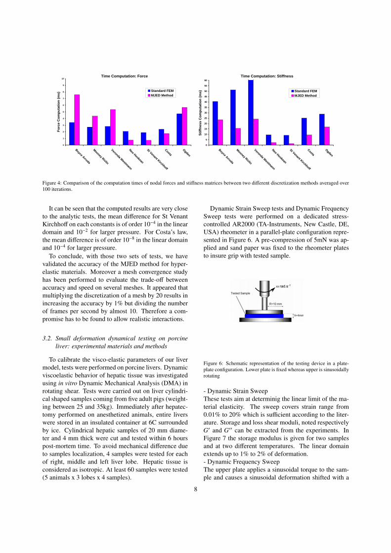
Decreasing computation time of the assembly of thestiffness matrix and force vector is essential to reachreal-time simulation as this represents around 45% ofthe total time needed in one step. Therefore we firstcompared our implementation with the classical FEMmethod explained in [21], referred to as ”StandardFEM”, both implemented in SOFA1. The results aregiven in Figure 4. We measured the time elapsed for thecomputation of the nodal forces and the stiffness ma-trices averaged over 100 iterations. We simulated the

1SOFA is an Open Source medical simulation software availableat www.sofa-framework.org

deformation of a cube with 20 700 tetrahedra and 4300nodes. For all modes implemented the proposed strat-egy is definitely more efficient than the standard FEM,up to five times as fast for St Venant Kirchhoff material.

Second, two sets of comparisons have been made tocheck the accuracy of the MJED. A first set of tests com-pares the node positions after a specified deformationbetween our simulation and the Open Source softwareFEBio (version 1.1.7)2 where several elastic and hyper-elastic materials are implemented. The mean relativedifference is around 10−6 for every models tested.

A second set of tests has been performed with the an-alytical solution of a deformed cube on which a verticalpressure p is applied on its top face. To this end, we as-sume that the deformation gradient in the global x-y-zcoordinate system is ∇φ = diag(α, β, γ). The simulatedvalues of α, β, γ are compared to analytical solutions ofthe system:

eTz ∇φ Sh ez = p

eTx ∇φ Sh ex = 0

eTy ∇φ Sh ey = 0

Figure 5 shows the results in the non-linear domain,for St Venant Kirchhoff materials.

Figure 5: Analytical and computed results for α and γ for severalpressures, with a log-scale, on St Venant Kirchhoff elasticity

2FEBio is an opensource software package for FE analysis avail-able at mrl.sci.utah.edu

7

Time Computation: Force

0

1

2

3

4

5

6

7

8

9

10

Boyce Arruda

Mooney Rivlin

Veronda Westm

ann

Neo Hookean

St Venant Kirchhoff

Costa

Ogden

Fo

rce

Co

mp

uta

tio

n (

ms)

Standard FEMMJED Method

Time Computation: Stiffness

0

5

10

15

20

25

30

35

40

45

50

55

60

Boyce Arruda

Mooney Rivlin

Veronda Westm

ann

Neo Hookean

St Venant Kirchhoff

Costa

Ogden

Sti

ffn

ess

Co

mp

uta

tio

n (

ms) Standard FEM

MJED Method

Figure 4: Comparison of the computation times of nodal forces and stiffness matrices between two different discretization methods averaged over100 iterations.

It can be seen that the computed results are very closeto the analytic tests, the mean difference for St VenantKirchhoff on each constants is of order 10−4 in the lineardomain and 10−2 for larger pressure. For Costa’s law,the mean difference is of order 10−8 in the linear domainand 10−4 for larger pressure.

To conclude, with those two sets of tests, we havevalidated the accuracy of the MJED method for hyper-elastic materials. Moreover a mesh convergence studyhas been performed to evaluate the trade-off betweenaccuracy and speed on several meshes. It appeared thatmultiplying the discretization of a mesh by 20 results inincreasing the accuracy by 1% but dividing the numberof frames per second by almost 10. Therefore a com-promise has to be found to allow realistic interactions.

3.2. Small deformation dynamical testing on porcineliver: experimental materials and methods

To calibrate the visco-elastic parameters of our livermodel, tests were performed on porcine livers. Dynamicviscoelastic behavior of hepatic tissue was investigatedusing in vitro Dynamic Mechanical Analysis (DMA) inrotating shear. Tests were carried out on liver cylindri-cal shaped samples coming from five adult pigs (weight-ing between 25 and 35kg). Immediately after hepatec-tomy performed on anesthetized animals, entire liverswere stored in an insulated container at 6C surroundedby ice. Cylindrical hepatic samples of 20 mm diame-ter and 4 mm thick were cut and tested within 6 hourspost-mortem time. To avoid mechanical difference dueto samples localization, 4 samples were tested for eachof right, middle and left liver lobe. Hepatic tissue isconsidered as isotropic. At least 60 samples were tested(5 animals x 3 lobes x 4 samples).

Dynamic Strain Sweep tests and Dynamic FrequencySweep tests were performed on a dedicated stress-controlled AR2000 (TA-Instruments, New Castle, DE,USA) rheometer in a parallel-plate configuration repre-sented in Figure 6. A pre-compression of 5mN was ap-plied and sand paper was fixed to the rheometer platesto insure grip with tested sample.

Figure 6: Schematic representation of the testing device in a plate-plate configuration. Lower plate is fixed whereas upper is sinusoidallyrotating

- Dynamic Strain SweepThese tests aim at determinig the linear limit of the ma-terial elasticity. The sweep covers strain range from0.01% to 20% which is sufficient according to the liter-ature. Storage and loss shear moduli, noted respectivelyG′ and G′′ can be extracted from the experiments. InFigure 7 the storage modulus is given for two samplesand at two different temperatures. The linear domainextends up to 1% to 2% of deformation.- Dynamic Frequency SweepThe upper plate applies a sinusoidal torque to the sam-ple and causes a sinusoidal deformation shifted with a

8

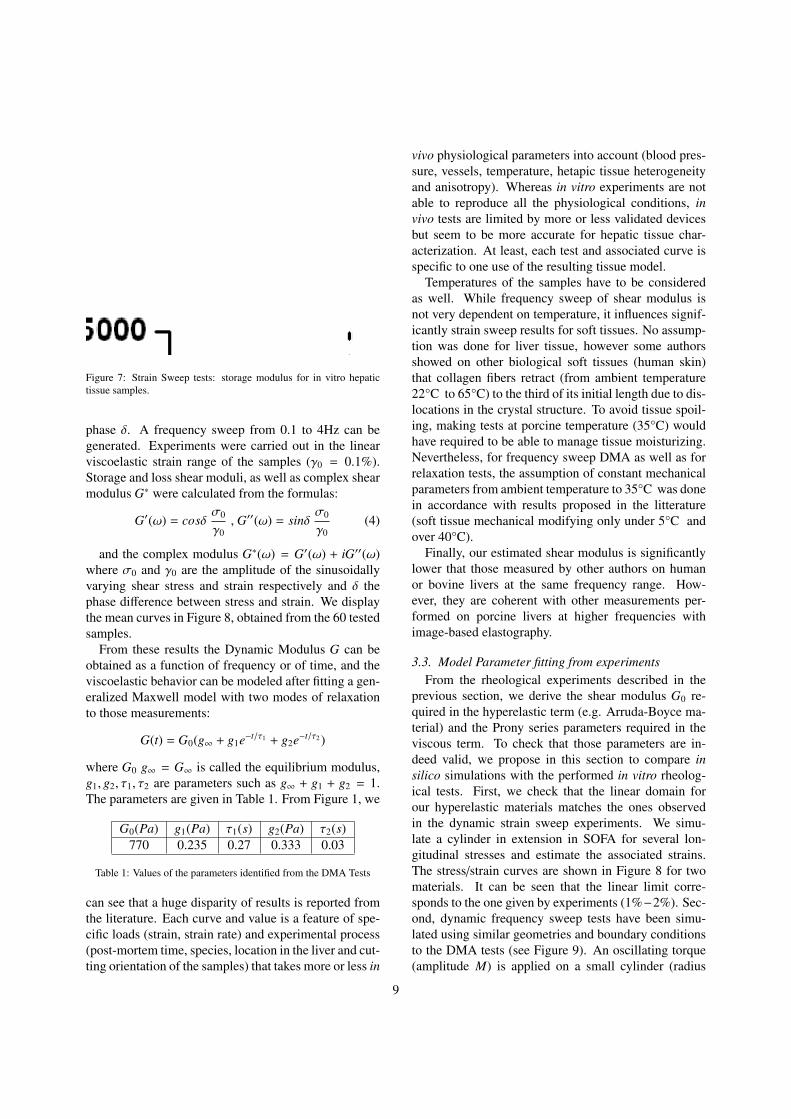
Figure 7: Strain Sweep tests: storage modulus for in vitro hepatictissue samples.

phase δ. A frequency sweep from 0.1 to 4Hz can begenerated. Experiments were carried out in the linearviscoelastic strain range of the samples (γ0 = 0.1%).Storage and loss shear moduli, as well as complex shearmodulus G∗ were calculated from the formulas:

G′(ω) = cosδσ0

γ0, G′′(ω) = sinδ

σ0

γ0(4)

and the complex modulus G∗(ω) = G′(ω) + iG′′(ω)where σ0 and γ0 are the amplitude of the sinusoidallyvarying shear stress and strain respectively and δ thephase difference between stress and strain. We displaythe mean curves in Figure 8, obtained from the 60 testedsamples.

From these results the Dynamic Modulus G can beobtained as a function of frequency or of time, and theviscoelastic behavior can be modeled after fitting a gen-eralized Maxwell model with two modes of relaxationto those measurements:

G(t) = G0(g∞ + g1e−t/τ1 + g2e−t/τ2 )

where G0 g∞ = G∞ is called the equilibrium modulus,g1, g2, τ1, τ2 are parameters such as g∞ + g1 + g2 = 1.The parameters are given in Table 1. From Figure 1, we

G0(Pa) g1(Pa) τ1(s) g2(Pa) τ2(s)770 0.235 0.27 0.333 0.03

Table 1: Values of the parameters identified from the DMA Tests

can see that a huge disparity of results is reported fromthe literature. Each curve and value is a feature of spe-cific loads (strain, strain rate) and experimental process(post-mortem time, species, location in the liver and cut-ting orientation of the samples) that takes more or less in

vivo physiological parameters into account (blood pres-sure, vessels, temperature, hetapic tissue heterogeneityand anisotropy). Whereas in vitro experiments are notable to reproduce all the physiological conditions, invivo tests are limited by more or less validated devicesbut seem to be more accurate for hepatic tissue char-acterization. At least, each test and associated curve isspecific to one use of the resulting tissue model.

Temperatures of the samples have to be consideredas well. While frequency sweep of shear modulus isnot very dependent on temperature, it influences signif-icantly strain sweep results for soft tissues. No assump-tion was done for liver tissue, however some authorsshowed on other biological soft tissues (human skin)that collagen fibers retract (from ambient temperature22°C to 65°C) to the third of its initial length due to dis-locations in the crystal structure. To avoid tissue spoil-ing, making tests at porcine temperature (35°C) wouldhave required to be able to manage tissue moisturizing.Nevertheless, for frequency sweep DMA as well as forrelaxation tests, the assumption of constant mechanicalparameters from ambient temperature to 35°C was donein accordance with results proposed in the litterature(soft tissue mechanical modifying only under 5°C andover 40°C).

Finally, our estimated shear modulus is significantlylower that those measured by other authors on humanor bovine livers at the same frequency range. How-ever, they are coherent with other measurements per-formed on porcine livers at higher frequencies withimage-based elastography.

3.3. Model Parameter fitting from experimentsFrom the rheological experiments described in the

previous section, we derive the shear modulus G0 re-quired in the hyperelastic term (e.g. Arruda-Boyce ma-terial) and the Prony series parameters required in theviscous term. To check that those parameters are in-deed valid, we propose in this section to compare insilico simulations with the performed in vitro rheolog-ical tests. First, we check that the linear domain forour hyperelastic materials matches the ones observedin the dynamic strain sweep experiments. We simu-late a cylinder in extension in SOFA for several lon-gitudinal stresses and estimate the associated strains.The stress/strain curves are shown in Figure 8 for twomaterials. It can be seen that the linear limit corre-sponds to the one given by experiments (1%−2%). Sec-ond, dynamic frequency sweep tests have been simu-lated using similar geometries and boundary conditionsto the DMA tests (see Figure 9). An oscillating torque(amplitude M) is applied on a small cylinder (radius

9

Linear Limit

Storage G' and Loss G'' moduli: Comparison with rea l data

10

110

210

310

410

510

610

710

810

0,1 1 10

Frequency (Hz)

Mod

uli (

Pa)

G' experimentG' simulationG'' experimentG'' simulation

Figure 8: (Left) Longitudinal stress/strain curves obtained with a cylinder for Boyce Arruda and St Venant Kirchhoff materials. (Right) Comparisonof the simulated values with the data obtained by DMA testing. The moduli are given on a x-log scale. The material is St Venant Kirchhoff, similarvalues are found for other materials.

r = 10mm, height h = 4mm) at various frequencies ω.The amplitude of the torque is chosen so as to stay in thelinear domain. The angle of rotation θ of the cylinder ismeasured as a function of time. This angle describesa sinusoidal curve which follows the torque amplitudewith a shifted phase δ. Specific constraint is applied onthe top cylinder nodes to enforce a pure rotation of thosenodes (as to reproduce the pure grip of sand paper).

Figure 9: (Left) Cylinder used for the simulation of shear deformation.(Pink) Rotating top nodes. (Blue triangles) Cylinder with parametersof the liver. (Blue dots) Fixed points.

Applying the classical formulas:

σ(t) =2Mπ r3 and γ(t) =

r θ(t)h

and equations (4) we can estimate the values of the stor-age and loss moduli to be compared with experimen-tal data. It can be seen in Figure 8 that the simulationmanages to capture the viscous behavior of the liver forsmall deformations with a mean relative error of 5%.Given the fit errors and the standard deviation of thevalues obtained with the DMA tests, this mean error isreasonably good.

3.4. Poro-hyperelasticity simulationWe have implemented the porous component in our

model using parameters based on Kerdok’s [18] experi-mental data as shown in Table 2.

f w K0(Pa) Klim(kPa) κ(m4/Ns)0.5 400 2.2 20

Table 2: Values of the parameters used for porosity component

In order to qualitatively check the accuracy of ourimplementation, we simulated a liver composed of twocomponents: Arruda-Boyce hyperelasticity and poros-ity. From time t=0s, gravity is uniformly applied to theliver while several selected vertices of a plane are fixed(representing the ligament and veins). The simulatedfluid pressure field during the deformation is shown inFigure 10 as a color map, ranging from dark blue (initialpressure) to red (highest pressure). Highest pressure inthe fluid occurs when the liver is compressed either bygravity (diffusion starts at the top) or by elastic reaction(diffusion starts at the bottom).

3.5. Complete Liver ModelTo describe the influence of each component in the

complete model, several simulations were performedusing the same liver mesh (1240 vertices and 5000tetrahedra), same parameters, under the same constantgravity force, and with a fifth-order Arruda-Boycematerial [28]. The liver mesh has been segmentedfrom a CT scan image and meshed with the GHS3Dsoftware. An Euler implicit time integration schemeis used with a time step of 0.07s, the linear equationsbeing solved with a conjugated gradient algorithm. As

10

P=0(Pa) P=100(Pa)

t = 0s t = 2s t = 4s

Figure 10: Pressure field of the porous component on a liver under gravity

Maximum Amplitudes Poro-hyperelasticity

Initial state / Final stateMaximum Amplitudes Visco-hyperelasticity

Figure 11: Addition of viscosity or porosity to hyperelasticity: Comparison of the maximum amplitudes and final states. (Black) Initial position,(Blue) Hyperelastic liver, (Pink) Visco-hyperelastic liver, (Green) poro-hyperelastic liver.

boundary conditions, several nodes of the liver are fixedalong the vena cava and suspensive ligament. The liverdeforms under the action of gravity exceeding the linearlimit of the material. All computations were performedon a laptop PC with a Intel Core Duo processor at 2.80GHz (simulations are available in the video clip). Theliver motion could be described as a pendulum-likemotion around the equilibrium state until stabilization.

(i) Influence of the viscous componentAdding viscosity to hyperelasticity increases theamplitude of the oscillations as the material becomesless stiff. In constrast to an essentially hyperelasticmodel, the final state is much different from the initialstate (see Figure 11). Indeed, the use of Prony seriesleads to a multiplication of the SPK tensor by 1 −

∑ak

at infinite time, which decreases the resistance of theliver. The frame rate is around 13 FPS against 14 FPSfor hyperelasticity alone. We did not reach the ideal25 FPS needed for real-time interaction. However the

implicit integration scheme allows larger time step(0.3s for instance) which speeds up the simulationand makes user interactions efficient. High amount ofextension and compression are possible which may besomewhat unrealistic, therefore the porous componentis necessary to control the amount of viscosity.

(ii) Influence of the porous componentAdding porosity to visco-hyperelasticity prevents theliver from having unrealistic large deformations. Themaximum amplitude is in between the hyperelasticityalone and the visco-hyperelasticity. The deformationis no longer isotropic and changes over time. Theaddition of this component decreases the computationalefficiency (6 FPS) since a semi-implicit integrationscheme is used for the porous component. Becauseof the fast variation of the explicit term J/J, the timestep has to be decreased to 0.15s. On our laptopPC, the simulation is still fluid enough to allow userinteractions.

11

4. Discussion

In this paper we have proposed an innovative methodto discretize hyperelastic materials on finite elementmeshes. The MJED method is fully general and requiresthe user to provide a decomposition of the strain energyinto simple terms. With this formulation, a number ofprecomputations can be performed to speed-up the as-sembly of stiffness matrices.

For the complete liver model, Arruda-Boyce materialwas chosen based on Kerdok’s observations [18] that theparenchyma is best represented by a 8-chain rubber likeelastic model. But alternative materials such as MooneyRivlin or Ogden could be also employed, whereas aCosta material is better suited for cardiac modeling. Inthe future, we are planning to perform additional strainsweep static tests in order to better characterize the hy-perelastic behavior of the liver. One improvement ofour model would be to add the influence of the Glissoncapsule which acts as a membrane surrounding the liverparenchyma. However rheological experiments of thatcapsule are difficult to perform because it is very thin,other type of experiments such as tensile testing couldbe considered. Another avenue of research would be tocouple the liver perfusion model with the simulation ofblood flow inside the two liver veinous systems.

We have also shown in section 3.3 that some pa-rameters of the liver model can be identified based ondynamic mechanical testing. Model personalizationis an important issue to create patient-specific simula-tions and we believe that ultrasound or MR elastometrycould be used for in vivo characterization of liver visco-elasticity. However such experiments are only valid forsmall deformations since they are non-invasive.

For full user interaction, it is required to reach at least25 FPS. For our visco-hyperelastic liver model, we werestill able to have a reasonable interaction despite a framerate of 13 by increasing the time step to 0.3s. Note thatusing implicit time integration schemes helped to ob-tain realistic behavior, whereas using explicit schemeswith much lower time steps and large frame rate lead tovery damped motion. For instance, the same hyperelas-tic model implemented with an explicit Runge Kutta 4solver could not be stabilized after the first interactioneven for a small time step (0.01s), and reaching only11 FPS. Thus, to have a robust simulation, no explicitsolver could be chosen.

There are several ways to improve the computationalefficiency (besides applying Moore’s law). First, theporosity computation could be computed in parallelwith the mechanical computation. Second, the assem-bly of stiffness matrices and the solution of linear sys-

tems of equations could be done on the GPU as alreadydemonstrated by several authors[12]. Finally, the pro-jection on reduced basis as shown in [8] could decreasethe size of the linear system to be solved at each timestep.

5. Conclusion

In this paper, we have introduced an efficient methodto assemble stiffness matrices for complex biomechan-ical material which compares favorably with the stan-dard FEM method. We have also proposed a poro-visco-hyperelastic liver model suitable for real-time interac-tion which is, up to our knowledge, among the mostrealistic ones in the literature. Several model param-eters have been identified from rheometric tests per-formed on 60 samples from porcine livers and a valida-tion study has been conducted to reproduce those testswell. Finally, the influence of each mechanical compo-nent has been evaluated. Despite those advances, muchresearch needs to be done to achieve a realistic liversurgery simulation including the modeling of liver con-tact with neighboring structures, the influence of breath-ing and cardiac motion, the simulation of hepatic resec-tion, bleeding and suturing.

Appendix A. MJED method

The strain energies Wkh = f k(J)gk(I) are derived with

respect to the points Qi to obtain nodal forces, (de-scribed previously in equations 1) and the terms aresummed up for each k. To get this first derivative, weuse the same calculations as made by Delingette [22].

Combining ∇φ =

4∑i=1

QiDTi and Sk

h = 2∂gk(I)∂C

we obtain:

∂gk(I)∂Qi

= DTi Sk

h ∇φT and from

∂ f k(J)∂Qi

= f k′(J)∂J∂Qi

(A.1)where the derivative of the Jacobian is expressed as

∂J∂Qi

=1

6V0((Q j − Ql) ∧ (Qk − Ql))T (A.2)

we get nodal forces that only require the inputsf k, f k′, gk and Sk

h :

Fh,i = −V0

n∑k=1

f k′(J)gk(I)(∂J∂Qi

)T

+ f k(J)∇φ Skh Di

(A.3)

12

To obtain the stiffness matrix, we need to derive twicethe strain energy, or to derive the transpose of theforce. We start by deriving the first term of the force:f k′(J) ∂J

∂Qigk(I). We obtain three terms:

Gk =

(∂ f k ′(J)∂Q j

)T∂J∂Qi

gk(I)

Hk = f k′(J) ∂2 J∂Q j∂Qi

gk(I)

Ik = f k′(J)(∂gk(I)∂Q j

)T∂J∂Qi

(A.4)

which are easily written using equation (A.1) and thesecond derivative of the Jacobian:

∂2J∂Q j∂Qi

==1 − δi j

6V0

0 −c3 c2c3 0 −c1−c2 c1 0

(A.5)

with δi j the Kronecker delta and c = (c1, c2, c3) the edgevector opposing Qi and Q j.Let consider the second term of the force:f k(J)DT

i Skh ∇φ

T . As Di is constant, that alsoleads to three additional terms:

Λk =

(∂ f k(J)∂Q j

)TDT

i Skh ∇φ

T

Mk = f k(J) DTi Sk

h

(∂∇φT

∂Q j

)T

Rk = f k(J)(∂Sk

h∂Q j

Di

)T∇φT

(A.6)

Computation of Λk and Mk is straightforward using thedefinition of ∇φ which gives ∂∇φ

∂Q j= IdDT

j and equation(A.1). Rk is more complex and in the remainder the.k notation is dropped to simplify notations and derivethe expression component wise. We seek to determinea matrix whose elements are ∂Sab

∂Qvj

where a, b and v arein [1..3]. Including the matrix C in the chain rule weexpress this term as:

∂Sab

∂Qvj

=

3∑m,n=1

∂Sab

∂Cmn

∂Cmn

∂Qvj

But, using ∂Cmn∂Qv

j=

∑4u=1[Qv

u Dmj Dn

u + Qvu Dm

u Dnj ]

and ∇φmn =∑4

u=1 Qmu Dn

u and noticing moreover thatDm

j ∇φvn =[D j ⊗ (∇φT ev)

]mn

. We can finally computethe expressions to obtain the derivative with respect toQv

j:

∂S∂Qv

j=∂S∂C

:[D j ⊗ (∇φT ev) + (∇φT ev) ⊗ D j

]where ∂S

∂C is a fourth order tensor, applied to the matrix[D j ⊗ (∇φT ev) + (∇φT ev) ⊗ D j

]which is a second order

tensor (a matrix). Finally the derivative we seek is :

∂S∂Q j

Di =

3∑v=1

∂S∂Qv

jDi ⊗ ev

Furthermore, we take advantage of the specific structureof the fourth order elasticity tensors. In all cases, thistensor can be written as a sum of two kinds of terms,

βk1 Ak

1 H Ak1 or βk

2 (H : Ak2) Ak

2

where βku are scalars, Ak

u are symmetric matrices, andA : B = tr(BT A) for any two matrices A,B. Each oneof those two kinds of terms leads to simpler expressionsof Rk, respectively:

f k(J) ∇φLk1(i, j) ∇φT and f k(J) ∇φLk

2(i, j) ∇φT (A.7)

where Lk1(i, j) and Lk

2(i, j) are the linear matrices Lk1(i, j) = βk

1

(Ak

1 Di ⊗ D j Ak1 + Ak

1(D j · Ak1 Di)

)Lk

2(i, j) = 2βk2

(Ak

2 D j ⊗ Di Ak2

)(A.8)

which are constant in most cases.To conclude, the stiffness matrix is:

Kh,i j =∂2W(TP)∂Qi∂Q j

= V0

∑k

(Gk +Hk +Ik +Λk +Mk +Rk)

(A.9)

Appendix B. Combining MJED and Prony series

It consists in adding to the hyperelastic stress tensorSv some time dependent stresses:

α(t) = α∞ +∑

i

αie−t/τi with

α∞ +∑

i

αi

= 1

At time n the visco-hyperelastic SPK tensor Snv can be

written as:Sn

v = Snh −

∑i

γni

γni = aiSn

h + biγn−1i where ai =

∆t αi

∆t + τiand bi =

τi

∆t + τi

∆t is the time step used for discretization and has to bethe same as the time step for any solvers during the sim-ulation. Therefore, we need to compute the total secondPiola-Kirchoff stress tensor Sn

h. This is done by comput-ing the inverse deformation gradient :

Snh = ∇φ−1

∑k

( f k′(J)gk(I)J∇φ−T + f k(J)∇φSkh)

13

where ∇φ−1 =(∑4

l=1 Pl ⊗∂J∂Ql

)/J.

The visco-hyperelastic nodal forces are therefore relatedto the hyperelastic ones by

Fnv,i = Fn

h,i + V0∇φ∑

i

γni Di

Moreover, once we have γn−1i the stiffness matrix is also

slightly updated from its hyperelastic formulation:

Knv,i j = Kn

h,i j

1 −∑k

ak

− V0DTj

∑k

bkγn−1k

DiId

Appendix C. pseudo-code of the MJED method

To compute the FEM formulation, three functions arenecessary to input into the solvers: an initialization , thecomputation of the force vector and finally the computa-tion of the stiffness matrix. We start with the init() func-tion (Algorithm 1) which loads the mesh, initializes thevariables and precomputes some quantities. This func-tion is only called once, before the simulation starts.Then we build the Force Vector (Algorithm 2) for ev-ery tetrahedron, and at each time step. And finally wecompute the stiffness matrices (Algorithm 3 for everytetrahedron, at each time step (depending on the solverused).

Algorithm 1 init() function1: Load the mesh and get the topology (tetrahedra,

vertices, edges ...)2: for every tetrahedron i do3: Get the reference points position in the tetrahe-

dron, P j

4: Calculate the reference volume V05: Calculate the Shape Vectors D j

6: for every edge with vertices u and v do7: Compute the linear matrices Lk(u, v) (see

equation A.8)8: end for9: end for

Acknowledgements

This work is partially funded by the European PASS-PORT project (Patient-Specific Simulation for Pre-Operative Realistic Training of Liver Surgery) FP7-ICT-2007- 223894

[1] H. Delingette, N. Ayache, Soft tissue modeling for surgery simu-lation, in: Computational Models for the Human Body, Elsevier,2004, pp. 453–550.

Algorithm 2 addForce() function1: for every tetrahedron i do2: Get the current points position in the tetrahedron,

Q j

3: Compute the Deformation Gradient ∇Φ

4: Compute the Cauchy-Green Tensor C5: Compute the Jacobian J6: for every vertex j do7: Compute the first derivative of the Jacobian

∂J∂Q j

(see equation A.2)8: end for9: for every k of the decomposition do

10: Get fk, f ′k , f ′′k , gk, and Sk

11: end for12: for every vertex j do13: Compute the Force F j summing the contri-

butions from the decomposition (see equationA.3)

14: end for15: end for

Algorithm 3 addDForce() function1: for every tetrahedron i do2: for every edge with vertices u and v do3: Compute the second derivative of the Jacobian

∂2 J∂Qu∂Qv

(see equation A.5)4: for every k of the decomposition do5: Calculate Gk, Hk, Ik, Λk, Mk and Rk using

Lk(u, v) (equations A.4, A.6 and A.7)6: end for7: Compute the Stiffness Matrix Kuv (see equa-

tion A.9)8: end for9: end for

14

[2] D. Hawkes, D. Barratt, J. Blackall, C. Chan, P. Edwards,K. Rhode, G. Penney, J. McClelland, D. Hill, Tissue deforma-tion and shape models in image-guided interventions: a discus-sion paper, Medical Image Analysis 9 (2) (2005) 163 – 175.

[3] A. I. Veress, G. T. Gullberg, J. A. Weiss, Measurement ofstrain in the left ventricle during diastole with cine-mri and de-formable image registration, Journal of Biomechanical Engi-neering 127 (7) (2005) 1195–1207.

[4] S. Cotin, H. Delingette, N. Ayache, A hybrid elastic model al-lowing real-time cutting, deformations and force-feedback forsurgery training and simulation, The Visual Computer 16 (8)(2000) 437–452.

[5] D. L. James, D. K. Pai, ArtDefo accurate real time deformableobjects, in: Computer Graphics (SIGGRAPH), 1999, pp. 65–72.

[6] M. Muller, J. Dorsey, L. McMillan, R. Jagnow, B. Cutler, Stablereal-time deformations, in: SCA ’02: Proceedings of the 2002ACM SIGGRAPH/Eurographics Symposium on Computer An-imation, 2002, pp. 49–54.

[7] M. Nesme, Y. Payan, F. Faure, Efficient, physically plausiblefinite elements, in: Eurographics 2005, August, 2005, TrinityCollege, Dublin, Ireland, 2005.

[8] J. Barbic, D. L. James, Real-time subspace integration for St.Venant-Kirchhoff deformable models, ACM TOG (SIGGRAPH2005) 24 (3) (2005) 982–990.

[9] G. Picinbono, H. Delingette, N. Ayache, Non-LinearAnisotropic Elasticity for Real-Time Surgery Simulation,Graphical Models 65 (5) (2003) 305–321.

[10] J. Teran, S. Blemker, V. N. T. Hing, R. Fedkiw, Finite vol-ume methods for the simulation of skeletal muscle, in: Euro-graphics/SIGGRAPH Symposium on Computer Animation, SanDiego, California, 2003, pp. 68–74.

[11] K. Miller, G. Joldes, D. Lance, A. Wittek, Total lagrangian ex-plicit dynamics finite element algorithm for computing soft tis-sue deformation, Communications in Numerical Methods in En-gineering 23 (2006) 121–134.

[12] Z. Taylor, O. Comas, M. Cheng, J. Passenger, D. Hawkes, D. .Atkinson, S. Ourselin, On modelling of anisotropic viscoelas-ticity for soft tissue simulation: numerical solution and gpu ex-ecution, Medical Image Analysis 13 (2009) 234–244.

[13] H. Yamada, Strength of Biological Materials, Williams andWilkins Co, 1970.

[14] M. Ottensmeyer, Tempest 1-d: an instrument for measuringsolid organ soft tissue properties, Experimental Techniques26 (3) (2002) 48–50.

[15] D. Valtorta, E. Mazza, Dynamic measurements of soft tissue vis-coelastic properties with a torsional resonator device, MedicalImage Analysis 9 (5) (2005) 481–490.

[16] N. P. J. Oudry, S. Chatelin, L. Sandrin, A. Allemann, L. Soler,R. Willinger, In vivo liver tissue mechanical properties by tran-sient elastography: Comparison with dynamic mechanical anal-ysis, International Research Council on Biomechanics of Injury2009.

[17] Z. Liu, L. Bilston, Large deformations shear properties of livertissue, Biorheology 39 (6) (2002) 735–742.

[18] A. E. Kerdok, Characterizing the nonlinear mechanical responseof liver to surgical manipulation, Ph.D. thesis, Harvard Univer-sity (2006).

[19] G. Joldes, A. Wittekemail, K. Miller, Suite of finite element al-gorithms for accurate computation of soft tissue deformation forsurgical simulation, Medical Image Analysis 13 (6) (2009) 912– 919.

[20] J. Weiss, B. Maker, S. Govindjee, Finite element implemen-tation of incompressible, transversely isotropic hyperelasticity,Computer Methods in Applied Mechanics and Engineering 135(1996) 107–128.

[21] C. Zienkiewicz, R. Taylor, The Finite Element Method, Volume2 : Solid Mechanics, Butterworth-Heinemann, 2000.

[22] H. Delingette, Triangular springs for modeling nonlinear mem-branes, IEEE Transactions on Visualization and ComputerGraphics 14 (2) (2008) 329–341.

[23] R. W. D. Veronda, Mechanical characterization of skin finite de-formations, Journal of Biomechanics 3 (1) (1970) 111–124.

[24] J. Teran, E. Sifakis, S. S. Blemker, V. Ng-Thow-Hing, C. Lau,R. Fedkiw, Creating and simulating skeletal muscle from thevisible human data set, IEEE Transactions on Visualization andComputer Graphics 11 (3) (2005) 317–328.

[25] J. Kim, M. A. Srinivasan, Characterization of viscoelastic softtissue properties from in vivo animal experiments and inverse feparameter estimation, in: Medical Image Computing and Com-puter Assisted Intervention (MICCAI), LNCS, Palm Springs,USA, 2005.

[26] S. Raghunathan, D. Evans, J. L. Sparks, Poroviscoelastic mod-eling of liver biomechanical response in unconfined compres-sion, Annals of Biomechanical Engineering 38 (5) (2010) 1789–1800.

[27] H. Xiao, L. Chen, Hencky’s elasticity model and linear stress-strain relations in isotropic finite hyperelasticity, Acta Mechan-ica 157 (2002) 51–60.

[28] E. Arruda, M. Boyce, A three-dimensional constitutive modelfor the large stretch behavior of rubber elastic materials, J.Mech. Phys. Solids 41 (2) (1993) 389–412.

15