A Penetration-Based Finite Element Method for Hyperelastic

A Penetration-Based Finite Element Method for Hyperelastic

Three-Dimensional Biphasic Tissues in Contact

by

Kerem Ün

A Thesis Submitted to the Graduate

Faculty of Rensselaer Polytechnic Institute

in Partial Fulfillment of the

Requirements for the Degree of

DOCTOR OF PHILOSOPHY

Major Subject: Biomedical Engineering

Approved by theExamining Committee:

____________________________________Robert L. Spilker, Thesis Advisor

____________________________________John B. Brunski, Member

____________________________________Mark H. Holmes, Member

____________________________________Mark S. Shephard, Member

Rensselaer Polytechnic InstituteTroy, New York

April 2002(For Graduation May 2002)

Table of Contents

page

Table of Contents .. .................................................................. iii

List of Tables ......... .................................................................. vi

List of Figures........ ................................................................. vii

Acknowledgements ................................................................ xiii

Abstract.................. ..................................................................xv

Chapter1: Introduc ....................................................................1

1.1 Prologue ........

1.2 Articular Cart

1.3 Cartilage Stud

1.4 Finite Elemen

1.5 Objective and

Chapter 2: Biphasi

2.1 Introduction...

2.2 Constitutive E

2.3 Cartilage Mate

Chapter 3: Nonline

3.1 Introduction...

3.2 Nonlinear Ela

3.3 Constitutive M

Chapter 4: Finite E

4.1 Introduction...

4.2 Velocity-Press

4.3 Weak Form ...

4.4 Linear Formul

.........................................

.........................................

.........................................

........................................

.........................................

tion .................................

iii

.............................................................................................................1

ilage .....................................................................................................1

ies ........................................................................................................4

t Formulations .....................................................................................7

Thesis Layout .....................................................................................9

c Theory of Articular Cartilage......................................................11

...........................................................................................................11

quations for Biphasic Mixture ..........................................................11

rial Properties ...................................................................................13

ar Elasticity......................................................................................15

...........................................................................................................15

sticity .................................................................................................15

odeling and Hyperelasticity .............................................................19

lement Formulation ........................................................................25

...........................................................................................................25

ure Formulation ................................................................................25

...........................................................................................................25

ation ..................................................................................................28

iv

4.5 Computer Implementation .......................................................................................32

4.5.1 Object Oriented Programming..........................................................................32

4.5.2 Implementation of the Linear Analysis.............................................................33

4.6 Nonlinear Formulation.............................................................................................36

4.6.1 Linearization .....................................................................................................38

4.6.2 Partial Linearization..........................................................................................43

4.6.3 Solution of the Nonlinear System .....................................................................45

4.6.4 Line Search .......................................................................................................49

4.7 Computer Implementation of the Nonlinear Analysis.............................................50

Chapter 5: Penetration Method......................................................................................54

5.1 Introduction..............................................................................................................54

5.2 Experimental Kinematics Data ................................................................................55

5.2.1 Visualization Techniques..................................................................................55

5.2.2 Interpolation through Discrete Kinematics Data ..............................................56

5.3 Biphasic Contact Boundary Conditions and Load Sharing .....................................57

5.4 Derivation of the Approximate Boundary Conditions.............................................59

5.5 Extension to Hyperelastic Solid Phase ....................................................................65

5.5.1 Application and Computer Implementation......................................................68

Chapter 6: Linear Examples...........................................................................................70

6.1 Introduction..............................................................................................................70

6.2 Canonical Examples ................................................................................................70

6.2.1 Results for Case CT ..........................................................................................72

6.2.2 Results for Case VT ..........................................................................................86

6.2.3 Evaluation of the Penetration Analysis Results ................................................87

6.3 Glenohumeral Analysis............................................................................................95

6.3.1 Approximate Contact Boundary Conditions.....................................................97

6.3.2 Humerus Results .............................................................................................100

v

6.3.3 The Glenoid Results........................................................................................105

6.3.4 Evaluation of the Glenohumeral Analysis Results .........................................105

Chapter 7: Nonlinear Examples ...................................................................................109

7.1 Introduction............................................................................................................109

7.2 Confined Compression Examples..........................................................................109

7.2.1 Creep ...............................................................................................................109

7.2.2 Stress Relaxation.............................................................................................112

7.2.3 Evaluation of the Confined Compression Analysis Results ...........................114

7.3 Glenohumeral Analysis..........................................................................................115

7.3.1 Approximate Contact Boundary Conditions...................................................115

7.3.2 Humerus Results .............................................................................................118

7.3.3 Glenoid Results ...............................................................................................118

7.3.4 Evaluation of the Glenohumeral Analysis Results .........................................123

Chapter 8: Summary, Conclusions and Future Research .........................................127

8.1 Summary................................................................................................................127

8.2 Future Research .....................................................................................................131

Bibliography ...................................................................................................................133

Appendix A: Derivation of the Tangent Stiffness for the Hyperelastic Material Law

..........................................................................................................................................142

Appendix B: Element Matrices of Nonlinear v-p Formulation .................................145

Appendix C: Justification for Disregarding the Tissue Curvature Effect in

Penetration Analysis ......................................................................................................146

vi

List of Tables

page

Table 1: The numerical procedure for the nonlinear problem ...........................................48

Table 2: The values of geometrical parameters defined in Figure 2 for cases CT and VT.

....................................................................................................................................71

vii

List of Figures

page

Figure 1: Organization of articular cartilage into different zones (adopted from [70]). ..... 2

Figure 2: Microstructure of articular cartilage (adopted from [70]). .................................. 3

Figure 3: Architecture of collagen fibers in articular cartilage (from[58]). ........................ 4

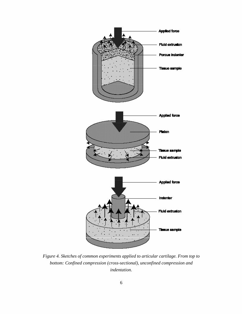
Figure 4. Sketches of common experiments applied to articular cartilage. From top to

bottom: Confined compression (cross-sectional), unconfined compression and

indentation. .......................................................................................................... 6

Figure 5: Symbols used in object oriented diagrams. ....................................................... 33

Figure 6: Analysis hierarchy of the implemented finite element code.............................. 34

Figure 8: Time integrator and system assembler hierarchy of the implemented finite

element code. ..................................................................................................... 35

Figure 9: Material hierarchy of the implemented finite element code. ............................. 36

Figure 10: Nonlinear analysis object in the analysis hierarchy......................................... 51

Figure 11: Nonlinear biphasic stiffness object in the stiffness contributor hierarchy....... 51

Figure 12: Nonlinear assembler object in the assembler hierarchy................................... 52

Figure 13: Nonlinear biphasic stiffness object in the stiffness contributor hierarchy....... 53

Figure 14: Graphical depiction of the idea behind penetration method............................ 54

Figure 15: Picture of overlapping cartilage models as obtained from the solid modeler

(top). Definitions of geometric parameters in overlapped models(bottom). ..... 60

Figure 16: Problem definition and geometry for the 2-D biphasic contact and 3-D

penetration-based analyses. Cartilage layers (dark gray) are attached to rigid

bone (light gray). A force is applied along the axis of symmetry. The centerline

thickness of layer A and layer B, and radii of curvature are defined. ............... 71

Figure 17: Case CT-CP, comparison of pressure and normal elastic traction distribution

on layers A and B, t = 1 sec............................................................................... 75

viii

Figure 18: Case CT-VP, comparison of pressure and normal elastic traction distribution


Figure 19: Case CT-CP, the axial displacement at the contact interface of layers A and B,

t = 1 sec.............................................................................................................. 76

Figure 20: Case CT-VP, the axial displacement at the contact interface of layers A and B,

t = 1 sec.............................................................................................................. 76

Figure 21: Case CT-CP, the normal velocity at the contact interface of layers A and B,

t = 1 sec.............................................................................................................. 77

Figure 22: Case CT-VP, the normal velocity at the contact interface of layers A and B,

t = 1 sec.............................................................................................................. 77

Figure 23: Case CT-CP, tissue A, comparison of the normal elastic traction with the shear

stress components in the planes along the normal direction, t = 1 sec.............. 78

Figure 24: Case CT-VP, tissue B, comparison of the normal elastic traction with the shear

stress components in the planes along the normal direction, t = 1 sec.............. 78

Figure 25: Case CT-CP, tissue A, total normal traction distribution from 3D penetration

compared with 2D contact finite element analysis result, t = 1 sec. ................. 79

Figure 26: Case CT-VP, tissue B, total normal traction distribution from 3D penetration


Figure 27: Case CT-CP, tissue B, pressure distribution from 3D penetration compared

with 2D contact finite element analysis result, t = 1 sec. .................................. 80

Figure 28: Case CT-VP, tissue B, pressure distribution from 3D penetration compared


Figure 29: Case CT-CP, tissue A, normal elastic traction distribution from 3D penetration


Figure 30: CT-CP, tissue B, normal elastic traction distribution from 3D penetration


Figure 31: Case CT-VP, tissue A, normal elastic traction distribution from 3D penetration


Figure 32: Case CT-VP, tissue B, normal elastic traction distribution from 3D penetration


ix

Figure 33: Case CT-CP, tissue A, axial displacement from 3D penetration compared with

2D contact finite element analysis result, t = 1 sec. .......................................... 84

Figure 34: Case CT-CP, tissue B, axial displacement from 3D penetration compared with


Figure 35: Case CT-VP, tissue A, axial displacement from 3D penetration compared with


Figure 36: Case CT-VP, tissue B, axial displacement from 3D penetration compared with


Figure 37: Case CT-CP, normal velocity from 3D penetration compared with 2D contact

finite element analysis result, t = 1 sec.............................................................. 86

Figure 38: Case VT-CP, comparison of pressure and normal elastic traction distribution


Figure 39: Case VT-VP, comparison of pressure and normal elastic traction distribution


Figure 40: Case VT-CP, tissue A, total normal traction distribution from 3D penetration


Figure 41: Case VT-VP, tissue B, total normal traction distribution from 3D penetration


Figure 42: Case VT-CP, tissue B, pressure distribution from 3D penetration compared


Figure 43: Case VT-VP, tissue A, pressure distribution from 3D penetration compared


Figure 44: Case VT-CP, tissue A, normal elastic traction distribution from 3D penetration


Figure 45: Case VT-CP, tissue B, normal elastic traction distribution from 3D penetration


Figure 46: Case VT-VP, tissue A, normal elastic traction distribution from 3D penetration


Figure 47: Case VT-VP, tissue B, normal elastic traction distribution from 3D penetration


x

Figure 48: Case VT-CP, tissue A, axial displacement from 3D penetration compared with


Figure 49: Case VT-CP, tissue B, axial displacement from 3D penetration compared with


Figure 50: Case VT-VP, tissue A, axial displacement from 3D penetration compared with


Figure 51: Case VT-VP, tissue B, axial displacement from 3D penetration compared with


Figure 52: Shoulder geometry with glenoid and humerus cartilages. ............................... 96

Figure 53: Comparison of magnitude of the total traction (upper) and pressure (lower) on

the contact faces of humeral head (left) and glenoid (right) cartilages at an arm

elevation angle of 40˚. ....................................................................................... 98

Figure 54: Comparison of magnitude of the total traction (upper) and pressure(lower) on


elevation angle of 60˚. ....................................................................................... 99

Figure 55: Maximum tensile stress distribution on the contacting face of the humerus at

arm elevations of 40˚ (top left), 50˚ (top right) and 60˚ (bottom). .................. 101

Figure 56: Maximum tensile stress distribution on the bone interface of the humerus at

arm elevations of 40˚ (top left), 50˚ (top right) and 60˚ (bottom). .................. 102

Figure 57: Maximum compressive stress distribution on the bone interface of the

humerus at arm elevations of 40˚ (top left), 50˚ (top right) and 60˚ (bottom). 103

Figure 58: Maximum shear stress distribution on the bone interface of the humerus at arm

elevations of 40˚ (top left), 50˚ (top right) and 60˚ (bottom). ......................... 104

Figure 59: Maximum tensile stress distribution on the contacting face of the glenoid at

arm elevations of 40˚ (left), 50˚ (center) and 60˚ (right). ................................ 106

Figure 60: Maximum tensile stress distribution on the bone interface of the glenoid at arm

elevations of 40˚ (left), 50˚ (center) and 60˚ (right). ....................................... 106

Figure 61: Maximum compressive stress distribution on the bone interface of the glenoid

at arm elevations of 40˚ (left), 50˚ (center) and 60˚ (right). ............................ 107

Figure 62: Maximum shear stress distribution on the bone interface of the glenoid at arm

elevations of 40˚ (left), 50˚ (center) and 60˚ (right). ....................................... 107

xi

Figure 63: The finite element mesh used in confined compression problems ................ 110

Figure 64: Pressure as function of depth at various time point in CC-CR. Solid lines

indicate converged FD results while symbols are FE results. ......................... 111

Figure 65: Axial displacement as function of depth at various time point in CC-CR. Solid

lines indicate converged FD results while symbols are FE results. ................ 111

Figure 66: Axial stress as function of depth at various time point in CC-CR. Solid lines


Figure 67: Pressure as function of depth at various time point in CC-SR. Solid lines


Figure 68: Axial displacement as function of depth at various time point in CC-SR. Solid

lines indicate converged FD results while symbols are FE results. ................ 113

Figure 69: Axial stress as function of depth at various time point in CC-SR. Solid lines




elevation angle of 40˚ originating from nonlinear penetration procedure....... 116



elevation angle of 60˚ originating from nonlinear penetration procedure....... 117


arm elevations of 40˚ (top left), 50˚ (top right) and 60˚ (bottom) degrees. ..... 119


arm elevations of 40˚ (top left), 50˚ (top right) and 60˚ (bottom) degrees. ..... 120


humerus at arm elevations of 40˚ (top left), 50˚ (top right) and 60˚ (bottom)

degrees. ............................................................................................................ 121

Figure 75: Maximum shear stress distribution on the bone interface of the humerus at arm

elevations of 40˚ (top left), 50˚ (top right) and 60˚ (bottom) degrees. ............ 122


arm elevations of 40˚ (left) and 50˚ (right)...................................................... 124

xii

Figure 77: Maximum tensile stress distribution on the bone interface of the glenoid at arm

elevations of 40˚ (left) and 50˚(right). ............................................................. 124


at arm elevations of 40˚ (left) and 50˚ (right).................................................. 125


elevations of 40˚ (left) and 50˚ (right). ............................................................ 125

Figure C.1: The penetration distribution assigned to a curved surface where g denotes the

varying penetration field and R is the radius of curvature. Line segment of

length d takes the length d’ after penetration is applied. ................................. 146

xiii

Acknowledgements Every doctoral thesis, I believe, has a personal component that is not evident in its

scientific content. I always enjoyed reading the acknowledgements part of theses independent of subject to get a feel for the personal story behind them. It is like a dream coming true that I am writing that very special part of my own thesis now. And I am happy to have the opportunity to express my gratitude to those who made this thesis more than a scientific document with eight chapters.

I believe that every doctoral student sooner or later realizes that by far the most important factor for a successful doctoral work is a good advisor. I have been lucky to have such an advisor: Prof. Robert L. Spilker was a good advisor and the nicest person to work with. I am grateful to him for his guidance, support and for making a ‘doctor’ out of me. I would also like to thank Prof. John B. Brunski, Prof. Mark H. Holmes and Prof. Mark S. Shephard, my committee members, for their valuable input. It saddens me as much that I cannot express my gratitude to Dr. Peter S. Donzelli personally, as his unfortunate and untimely death in August, 2000. He was a great colleague and friend; I will always remember him.

Nobody has given me as much encouragement in various aspects of my life, including my doctoral study, as my mother, Ayla Ün. Although she was away from her son for more than 8 years she never complained. I am grateful to her for her loving care, patience and encouragement.

My brother Kerim was a great friend and supporter. He always understood me and supported me in stressful times. I greatly appreciate his love, care and friendship.

When spending a long time far away from home it is inevitable that one day the telephone rings and you hear some sad news from your beloved ones. I lost both of my grandparents while I was studying hard for my doctoral degree. I am sure that they would have been delighted to see my graduation day.

I guess, nobody could have been happier than my father, Dr. Resat Ün, to see me complete my degree to become, in his words, “the second Dr. Ün”. Unfortunately, 11th April, 1998 was one of those days when my office phone rang and I was told that we had lost him. My father was a paragon of honesty in his scientific and personal life, and I will try to follow his footsteps to the best of my ability. I dedicate this work to his beloved memory.

xiv

I am fortunate that during my graduate years I had much more fun moments than sad ones. As valuable to me as this degree are the friends that I made during this time. While every scientific work eventually becomes outdated, true friends never do. Arnold Oyola, Mehmet Baran and Dean Nieusma have been truly like brothers to me. They were always around at good times and bad times. I have greatly enjoyed the friendship of Mike Nathanson, Bülent Yegenoglu, Elena Martinova and Martin Martinov, Tasso Anagnastopoulos, Lale Ergene, and Bouchra Bouqata. Their presence made my life very colorful and I sincerely hope that I have had a similar impact on theirs.

Taiseung Yang and Echo Miller made my stay in the Computational Biomechanics Laboratory a lot of fun. I enjoyed our tea breaks and talking with them about a wide variety of scientific and non-scientific topics.

Last, but certainly not the least, I am grateful to Marella for her love, encouragement and support. She is the nourishment of my life; life is simply beautiful with her!

I am thankful to the Ministry of National Education of Turkey for making my study abroad possible through their scholarships. The financial support of NIH, NSF and Surdna Foundation is also gratefully acknowledged.

AbstractAdvancements in theoretical, computational and experimental methods have

enabled researchers to develop more refined and realistic models for articular cartilage. A

realistic numerical simulation of cartilage mechanics under in vivo conditions requires the

tissue layers to be modeled in contact, undergoing large deformation.

The objective of the current research is to develop an efficient finite element

procedure for numerical simulation of three-dimensional (3-D) biphasic cartilage layers

in contact. To achieve that objective, the penetration method is developed as a

preprocessing technique that makes use of experimentally measured joint kinematic data

to derive approximate contact boundary conditions. This process eliminates the

nonlinearity associated with contact mechanics, and enables independent analyses of the

contacting tissues. The derived boundary conditions provide the input to a finite element

procedure where the material and geometric nonlinearities, as well as the strain-

dependent permeability, of the tissue layers are taken into account through a biphasic

continuum model.

The linear and nonlinear versions of penetration-based biphasic finite element

analyses are critically evaluated using canonical problems, then applied to a physiological

example, namely the glenohumeral joint of the shoulder. This work represents the first

attempt to analyze contacting biphasic articular cartilage layers on physiological

geometries under finite deformation. This is a numerically challenging problem and

requires that conventional nonlinear solution procedures be improved. The research

therefore included an examination of alternate linearizations of the nonlinear problem and

line search techniques to stabilize the iterative solution scheme.

Both linear and nonlinear versions of this formulation have been implemented

into the object-oriented analysis framework, Trellis, of the Scientific Computation

Research Center at Rensselaer Polytechnic Institute using the C++ programming

language.

1

Chapter 1

Introduction

1.1 Prologue

The interest of humankind in the mechanism of the human system is a centuries-

old obsession that has attracted some of the brightest scientific minds of history,

including Aristotle, Leonardo da Vinci, Galileo Galilei and Helmholtz. Today this

interest is shared by an ever-growing number of scientists with an aim of thoroughly

understanding the mechanisms involved in function of the human body in order to

improve human life.

Biomedical engineering involves the application of engineering fundamentals to

biological sciences. Although fundamentally interdisciplinary, it is rapidly emerging as a

separate discipline. The existence of such a discipline is well justified by the fact that

today health sciences utilize more high technology than ever before. In fact, many

medical breakthroughs such as magnetic resonance imaging (MRI), artificial heart,

dialysis and orthopedic implants are a product of this interdisciplinary engineering work.

Biomechanics, an important branch of biomedical engineering, involves the

application of engineering mechanics in biological sciences. Within the diverse spectrum

of biomechanics, the mechanical behavior of various tissues is an important topic.

Soft tissues constitute an important component of mammalian physiology and

fulfill various mechanical functions. The flow of blood in the arteries, elasticity of veins,

arteries and articular cartilage are just a few examples of properties that are of vital

importance. In other cases, soft tissue mechanical properties are not of direct relevance

for normal function; however, they can be important to the reaction of tissue to external

effects. Brain trauma caused by impact, and the formation of pressure ulcers are

examples of such situations. As a result of the significance of mechanical function,

particularly in the cardiovascular and musculoskeletal systems, understanding and

characterizing the mechanical behavior of soft tissue has emerged as a critical component

of biomechanics.

1.2 Articular Cartilage

Diarthrodial joints such as the shoulder or the knee joint are characterized by the

presence of articular cartilage and a strong fibrous capsule lined with a metabolically

2

active synovium. Articular cartilage is the thin layer of soft tissue that covers the

contacting surfaces of bones in diarthrodial joints. Daily activities impose high contact

forces on diarthrodial joints [3] that are transmitted from one bone to the other through

these thin cartilage layers.

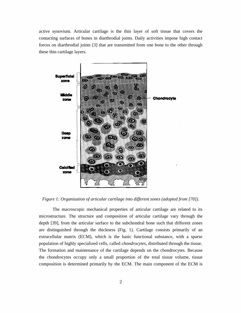
Figure 1: Organization of articular cartilage into different zones (adopted from [70]).

The macroscopic mechanical properties of articular cartilage are related to its

microstructure. The structure and composition of articular cartilage vary through the

depth [39], from the articular surface to the subchondral bone such that different zones

are distinguished through the thickness (Fig. 1). Cartilage consists primarily of an

extracellular matrix (ECM), which is the basic functional substance, with a sparse

population of highly specialized cells, called chondrocytes, distributed through the tissue.

The formation and maintenance of the cartilage depends on the chondrocytes. Because

the chondrocytes occupy only a small proportion of the total tissue volume, tissue

composition is determined primarily by the ECM. The main component of the ECM is

3

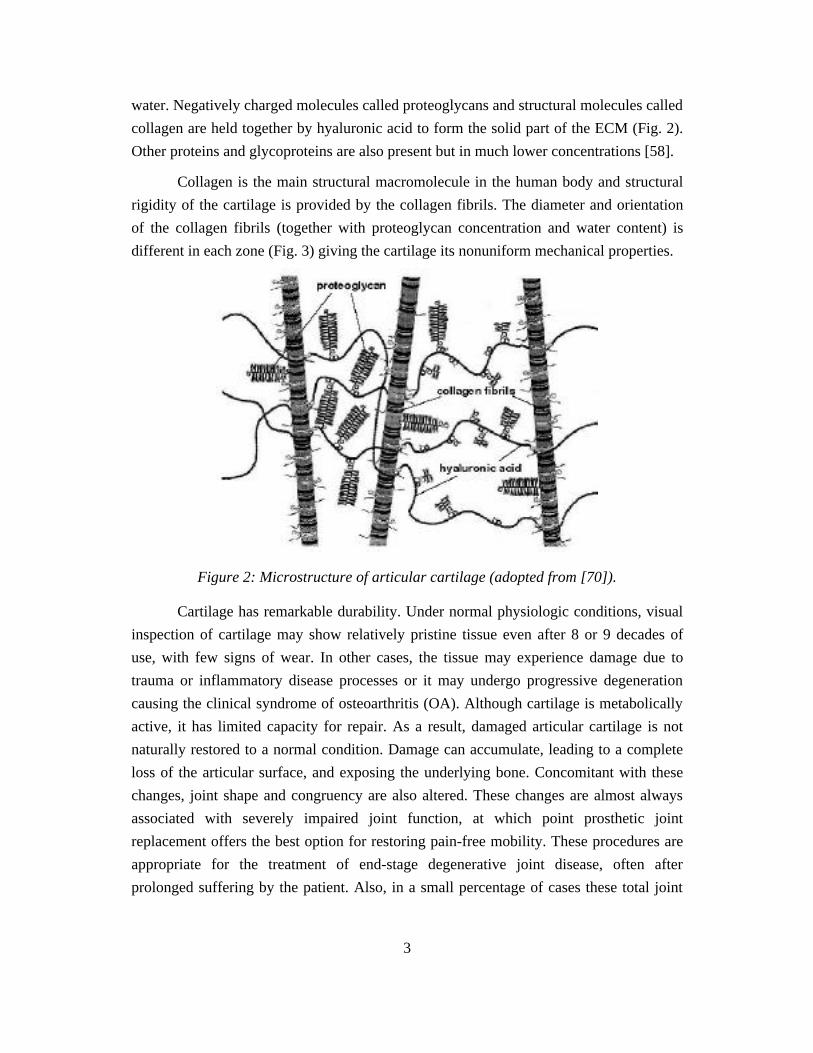
water. Negatively charged molecules called proteoglycans and structural molecules called

collagen are held together by hyaluronic acid to form the solid part of the ECM (Fig. 2).

Other proteins and glycoproteins are also present but in much lower concentrations [58].

Collagen is the main structural macromolecule in the human body and structural

rigidity of the cartilage is provided by the collagen fibrils. The diameter and orientation

of the collagen fibrils (together with proteoglycan concentration and water content) is

different in each zone (Fig. 3) giving the cartilage its nonuniform mechanical properties.

Figure 2: Microstructure of articular cartilage (adopted from [70]).

Cartilage has remarkable durability. Under normal physiologic conditions, visual

inspection of cartilage may show relatively pristine tissue even after 8 or 9 decades of

use, with few signs of wear. In other cases, the tissue may experience damage due to

trauma or inflammatory disease processes or it may undergo progressive degeneration

causing the clinical syndrome of osteoarthritis (OA). Although cartilage is metabolically

active, it has limited capacity for repair. As a result, damaged articular cartilage is not

naturally restored to a normal condition. Damage can accumulate, leading to a complete

loss of the articular surface, and exposing the underlying bone. Concomitant with these

changes, joint shape and congruency are also altered. These changes are almost always

associated with severely impaired joint function, at which point prosthetic joint

replacement offers the best option for restoring pain-free mobility. These procedures are

appropriate for the treatment of end-stage degenerative joint disease, often after

prolonged suffering by the patient. Also, in a small percentage of cases these total joint

4

replacements lack the durability of the normal joint. Biological and biomechanical studies

aimed at understanding the etiology of OA offer hope for the development of alternatives

to prosthetic joint replacements.

Figure 3: Architecture of collagen fibers in articular cartilage (from[58]).

1.3 Cartilage Studies

Characterizing the mechanical behavior of soft tissues is a critical step to gain

insight into human functional physiology. For cartilage, mechanical properties should be

related to occurrences and mechanisms of degenerative joint diseases. Knowledge

accumulated through integrated experimental, theoretical and computational research is

essential if biomechanics is to lead to improvement in diagnosis, treatment and

rehabilitation.

One of the main challenges in cartilage studies is to predict the deformation

behavior of cartilage. And the first ingredient to accomplish this is to determine a

constitutive law for cartilage. Constitutive laws describe mathematically the relation

between the loading and deformation of a material. A variety of constitutive laws have

been proposed for cartilage. Elastic models of cartilage have been used extensively,

particularly in early biomechanical studies. Viscoelastic models of different complexity

have also been proposed to account for the time-dependent deformation behavior. (See

[62] for a review.) Both of these approaches fail to account for the structure of cartilage

although they can provide good agreement with experimental deformation data in some

cases. Researchers recognized the importance of the interstitial fluid for some time, but it

was not until 1980 that the fluid phase was incorporated into the constitutive model of

cartilage. Mow et al. [63] proposed the superposition of a fluid continuum with a solid

5

continuum and used mixture laws [94] to derive the constitutive equations. This so-called

biphasic theory was consistent with respect to the load-bearing mechanism in cartilage

and the analytical results, based on an elastic solid phase and an inviscid fluid phase,

agreed well with experimental data for cartilage under small strains. In subsequent

studies, intrinsic viscoelasticity of the solid phase was also incorporated into the biphasic

theory [56]. The continuum representation of cartilage has been improved by considering

the stiffening caused by the Donnan effect of the charged particles in the cartilage matrix,

leading to the triphasic theory, where the third phase is the ions [52].

Material testing to determine the coefficients in a proposed constitutive law of

cartilage is usually through confined compression, unconfined compression and

indentation tests (see Fig. 4). To evaluate the coefficients, a solution of the biphasic

equations and constitutive law is required for the experimental configuration. In addition

to determining the material coefficients, combinations of these tests can provide cross-

validations of the constitutive law and biphasic model. Once a constitutive law is

confirmed, it is theoretically possible to predict cartilage deformation behavior without

the need for additional experiments.

Analytical solutions of the linear or nonlinear biphasic equations can only be

derived for a specialized geometry and loading conditions. Analytical solutions for short

and long-time response of biphasic cartilage have been derived for unconfined

compression [4] and indentation [57] experiments, both with displacement control (stress

relaxation) and force control (creep). However, these solutions are valid only for a

perfectly lubricated interface between the cartilage and the loading platen. The analytical

solution for confined compression has long been known from uniaxial consolidation in

soil mechanics [24]. Perturbation and integral transform solutions have been derived for

confined compression with strain-dependent permeability [41], for the canonical contact

of two biphasic layers [6, 50, 101, 102] and for rolling contact [8].

The limited number of cases amenable to analytical solution underscore the value

of numerical methods and the corresponding simulation tools in cartilage studies, as

described in the next section.

6

Figure 4. Sketches of common experiments applied to articular cartilage. From top to

bottom: Confined compression (cross-sectional), unconfined compression and

indentation.

7

1.4 Finite Element Formulations

Physiological soft tissue geometries represent complicated 3-D problem domains.

The general inhomogeneity and anisotropy of the tissue complicates the situation even

further. Analytical solution of such problems is not possible, and thus robust numerical

methods, such as the finite element method, are required to study tissues under realistic

physiological conditions.

Although the origin of the finite element method goes back to the 1940`s, it

gained wide popularity only after high performance computers became available as

research tools. The method has been increasingly employed in biological problems in the

last two decades where continuum models and their underlying partial differential

equations have been found applicable, and has been used extensively in soft tissue

mechanics.

The physiological situation in a diarthrodial joint involves two contacting layers

of articular cartilage, and in some cases three or more contacting bodies (e.g., the contact

between tibial plateau, femur and interposed meniscus). An ideal numerical simulation

therefore calls for a contact finite element analysis performed on the contacting cartilage

layer geometries, possibly incorporating inhomogeneity, anisotropy and finite

deformation. Although several attempts have been made to model cartilage layers in

contact through finite element methods, those analyses have either used the (less realistic)

elastic material law or been limited to certain experimental or canonical geometries [38,

73, 90, 91, 103]. One obvious reason for this is the high computational resources required

by a realistic 3-D biphasic contact analysis of the type mentioned above.

Different finite element formulations have been proposed based on the biphasic

model articular cartilage to study, mostly, canonical configurations too complex for

analytic solution. The alternate finite element formulations arise from the choices of

those governing equations to be satisfied exactly and those that are satisfied

approximately (i.e., in a weak sense). In the biphasic soft tissue problem, alternate

formulations originate additionally from options for treating the continuity constraint, and

options for eliminating one of the variables from the governing equations (such as

pressure or fluid velocity). Some formulations based on biphasic theory are comparable

to formulations from consolidation theory of soil mechanics, although the definition of

some parameters and their physical interpretation are different.

In the penalty method, the continuity equation is expressed in penalty form, and

continuity is enforced as the penalty parameter approaches infinity. Numerically, (since

8

we can not have an infinitely large number) the penalty parameter should be large enough

to enforce continuity but not so large that the system becomes ill-conditioned. Pressure is

then eliminated from the governing equations using the penalty form of continuity. Suh et

al. [83, 84] derived both linear and nonlinear axisymmetric versions of this formulation,

and used that formulation to study articular cartilage in experimental configurations.

In the mixed-penalty formulation, the penalty form of the continuity is added to

the weighted residual statement rather than used to eliminate the pressure from the

governing equations. Unlike the penalty formulation, pressure is a primary variable in

this approach and needs to be interpolated. Linear [82, 97] and nonlinear [2] versions of

this formulation have been applied to study cartilage deformation. An axisymmetric

contact formulation using this approach also has been implemented to study contact of

articular cartilage layers [26]. A mesh-free multiquadratic method based on the penalty

formulation has been proposed as an alternative to the classical finite element method

[44]. Recently, Suh et al. incorporated a viscoelastic solid phase with a mixed-penalty

based finite element formulation to model cartilage in confined [85] and unconfined

compression [86].

Another formulation that is used in cartilage mechanics is the hybrid formulation

which is similar to assumed stress methods proposed by Pian for elasticity problems [69].

In this method, the momentum equation of the mixture is exactly satisfied a priori by

choosing the shape functions for elastic stress and pressure properly. The continuity

equation, fluid momentum equation and the strain-displacement law, along with the

natural boundary conditions, are introduced into a weighted residual statement [96].

Levenston et al. [55] derived three nonlinear formulations of the poroelastic

theory based on three variational principles that make use of alternate penalized forms of

the internal energy. Two of the forms lead to alternate 3-field formulations where the

unknowns are solid phase velocity, pressure and relative velocity. The other form gives a

2-field formulation with solid phase velocity and relative velocity as unknowns.

Theories involving the additional (e.g. ion) phases, namely triphasic and

quadriphasic theories have also been incorporated into finite element methods [33, 43,

78, 87]. They have been generally limited to either small deformation cases or to

canonical geometries. It should be noted that without some simplifying assumptions,

theories involving an ion phase lead to a set of nonlinear governing equations even in the

absence of large deformations.

9

The velocity-pressure formulation [1] has been shown to be successful for 3-D

biphasic problems discretized using tetrahedral elements, and is the method of choice in

this thesis. A closely related formulation, namely displacement-pressure formulation is

also evaluated for the nonlinear analysis. Both formulations are covered in detail in

Chapter 4.

1.5 Objective and Thesis Layout

The on-going research, and advancements in the computer and experimental

technology have enabled researchers to develop more refined and realistic models for

articular cartilage. However, cartilage has still not been modeled under physiological

conditions, which require not only a proper constitutive law and physiological geometric

data, but also simulation of the in vivo mechanical environment. The objective of this

thesis research is to improve the existing work by modeling cartilage under in vivo

contact conditions. Here, we present a procedure where 3-D, biphasic, cartilage tissue

layers in contact are modeled using finite element methods and experimental kinematics

data. It is an interesting demonstration that what numerical or experimental studies alone

cannot accomplish can be achieved by combining the two. A simplified numerical

simulation of the biphasic contact is achieved by deriving approximate time-dependent

contact boundary conditions from experimental data and applying those within a finite

element scheme. The material and geometric nonlinearities, as well as the strain-

dependent permeability associated with the tissue layers are also taken into account.

Hence, the significance of the current work is that it constitutes the very first attempt for

the nonlinear 3-D numerical simulation of biphasic tissue layers under contact conditions.

Both the penetration method and the finite element procedures are implemented with a

object-oriented framework. Additional numerical precautions are taken to handle the

nonlinear contact simulation since it is a particularly challenging problem.

The thesis is organized as follows:

The biphasic theory of cartilage is outlined in Chapter 2 along with a description

of cartilage material properties.

Chapter 3 provides the background for the nonlinear analysis of cartilage.

Following an introduction to nonlinear elasticity, the basic principles for deriving

constitutive rules are briefly mentioned and the hyperelastic law used in the nonlinear

analysis of cartilage is described.

10

The linear and nonlinear finite element formulations are derived in detail in

Chapter 4. The computer implementation of these formulations within the object-oriented

finite element framework of the Scientific Computation Research Center at Rensselaer

Polytechnic Institute is also described.

Chapter 5 presents the penetration method, which makes use of experimental data

for approximate numerical simulation of tissue contact for both small and large

deformation.

The method is validated and small deformation examples on physiological

geometries are given in Chapter 6. The validation of the nonlinear finite element

formulation is given in Chapter 7 where large deformation examples on physiological

geometries are also presented.

Chapter 8 summarizes and evaluates the current work, and proposes directions for

future research.

11

Chapter 2

Biphasic Theory of Articular Cartilage

2.1 Introduction

The physics of continua is governed by conservation laws and restrictions

imposed by the second law of thermodynamics. In this chapter, after covering briefly the

conservation laws and the second law of thermodynamics, we will list the governing

equations of biphasic soft tissue and discuss their physical meanings. The chapter

concludes with the methods to determine the cartilage material properties.

2.2 Constitutive Equations for Biphasic Mixture

As described briefly in the previous chapter, articular cartilage can be represented

as a continuum solid matrix filled with an interstitial fluid. This biphasic structure plays a

important role in cartilage function; thus, when modeling cartilage as an engineering

material it is crucial to take its biphasic morphology into account.

Generally, two approaches are used to model a porous medium with filling liquid.

One approach is to average the governing continuum equations. This is an elaborate

process and has been done by Whitaker for porous media [99]. The averaging approach

appears to be more appropriate for soil mechanics problems where the solid phase

consists of relatively large particles compared to articular cartilage matrix. In soil

mechanics, the shape of the solid particles affect the averaging process whereas in

cartilage it is hard to define a “shape” for the collagen and proteoglycan molecules. The

characteristic lengths involved would not allow the fluid phase to be considered as a

uniform medium.

An alternative is to use continuum theories where each medium is treated as a

continuum, independent of the particle shape. While the shape of the particles making up

the solid matrix will have an effect on the solid phase constitutive equations, it will not

affect the general conservation equations.

Deformation of saturated porous media was first presented by Terzaghi [89] in a

one dimensional problem, and then extended to 3-D by Biot [12]. Their derivation was

based on empirical evidence that the fluid flow in porous media obeys a conduction-type

law (Darcy’s law), where the flow is proportional to the pressure gradient. Although in

12

practice identical to biphasic approach, consolidation theory takes the solid skeleton as

the problem domain and does not explicitly mention of the fluid phase as a second phase.

The interstitial fluid, the second phase of the soft tissue, makes up 70-80% of the

cartilage volume, and is known to be an important factor in the load bearing mechanism

of this tissue. Mow et al. [63] first took the fluid phase of cartilage into account when

deriving its constitutive equations to form the biphasic theory of soft tissue. They looked

at the problem from a continuum mechanics view point and used mixture theory [15, 16,

94] to derive the governing equations and constitutive law. In this approach, the solid and

fluid phases are considered separate overlapping continua. The individual phases, and the

mixture as a whole, have separate balance equations that, according to principle of

mixtures, should all have similar forms. In general mixture theory, mass, momentum,

angular momentum and energy transfer from one phase to the other is possible. Specific

to soft tissue, the phases are assumed to be immiscible, which simplifies mass balance.

The temperatures of each phase are assumed to be the same, so there is no heat exchange

between phases, a fact that simplifies energy balance.

Physically, the drag created by the movement of the fluid through the solid matrix

gives the tissue its viscoelastic properties. The following equations describe the biphasic

theory of soft tissue with the superscripts s and f referring to the solid and fluid phases,

respectively. The crucial assumption is that both phases of hydrated soft tissue are

incompressible, which results in a divergence-free, phase-averaged velocity. This serves

as the continuity equation for the biphasic tissue and given as,

∇ •f v f + svs( ) = 0, (1)

where are the phase volume fractions of the tissue and v denote the phase velocities.

Substituting Eq. (1) into the Clausius-Duhem inequality, and assuming an elastic solid

phase and inviscid fluid phase [1], provides the expressions for the solid and fluid phase

stresses:

s = − spI + E , (2)

f = − f p , (3)

where p is pressure and E is the elastic stress tensor corresponding to the deformation of

the solid phase. Momentum equations for each phase are expressed as,

∇ • + = 0, = s, f , (4)

13

where is the Cauchy stress tensor and is the momentum exchange between phases.

given by

s = − f = p∇ s + K v f − vs( ). (5)

In the above equation, K is the diffusive drag coefficient, related to the tissue

permeability through [53].

K =f( )2

. (6)

Equation (5) originates directly from the Clausius-Duhem inequality. Note that according

to Eq. (5), a momentum transfer from one phase to the other occurs only if the phases

have a relative velocity with respect to each other, and/or if the solid phase fraction has a

gradient in the tissue. Total stress is defined by adding the solid phase and fluid phase

stresses, Eq, (2) and Eq. (3) respectively

Tot = s + f = −pI + E (7)

As seen in Eqs. (2) and (3), the superposed continua approach leads to the rather

“unintuitive” result that pressure is shared between the phases. Physically, what the solid

phase experiences is the sum of the elastic stress and the pressure, i.e. the total stress.

Since hydrostatic pressure does not contribute to the failure of an elastic material, elastic

stress stands out as the most important quantity in cartilage mechanics. In fact, elastic

stress is attributed a special importance also in soil mechanics where it is called

effective stress [66].

In the finite element method, depending on the formulation chosen, the above

equations need to be satisfied either exactly or in integral sense.

2.3 Cartilage Material Properties

The determination of cartilage material properties has been a main focus in

cartilage research, and remains an active research area. For a mechanical analysis, the

material properties of interest are the elastic material properties and the tissue

permeability. For electromechanical models of cartilage [52] it is also necessary to

determine its electrochemical properties. The solid phase of the cartilage is usually

modeled as an elastic material, although some investigators are assessing the need to

include the intrinsic viscoelastic behavior of the solid phase to better capture the short

term behavior [46, 86]. Under large deformation, cartilage, soft tissues such as cartilage

are often modeled as hyperelastic, as discussed in detail in Chapter 3.

14

Early attempts mostly aimed at determining the Young`s modulus of the cartilage

at equilibrium. These involve usually an indentation experiment where the Young`s

modulus is calculated from the equilibrium deformation using the force, displacement

and available analytical solutions to the experimental configuration (See [62] for a

review). Similar analyses are still performed with more sophisticated experimentation

techniques [92].

Once the elastic properties of the tissue are known the permeability can be

determined using optimization techniques. Tabolt [88] describes a methodology where

the analytical solutions for confined and unconfined compression tests are used to

determine material properties as functions (polynomials of first or second order) of

measurable experimental quantities such as the surface stress. This response-surface

method less effective if the polynomial coefficients for both the elastic properties and

permeability are determined simultaneously.

A simultaneous estimation of Young`s modulus, Poisson`s ratio and permeability

is more complex because it constitutes an inverse problem. Mow et al. determine these

three parameters by inverting numerically the semi-analytical solution of the biphasic

indentation problem with a similarity principle. Other researchers have used this

approach since the indentation test is relatively easy to apply [9, 35].

The above methods assume the tissue to be homogeneous and return one

numerical value for each material parameter. If there is a variation in the material

properties the inverse problem is solved numerically. In this approach a finite element or

finite difference scheme is adapted and the material properties are determined at each

node. Inverse problems, by their nature, are ill-conditioned, nevertheless examples of

numerical methods to solve inverse problems with elastic [61] and biphasic [68, 75] laws

exist in the biomechanics literature.

Depth-dependent inhomogeneous elastic properties can be determined through

microscopy-based experimentation, too. This is usually accomplished by tracking the

chondrocytes through labeling their nuclei fluorescently [72] or using confocal

microscopy [36]. The locations of sparsely distributed chondrocytes before and after

deformation provide information about the strain levels at different depths.

In this work, uniform material properties (whether linear or nonlinear) are taken

from the literature, although the analysis program has the capability of handling spatially

varying material properties.

15

Chapter 3

Nonlinear Elasticity

3.1 Introduction

This chapter provides some background knowledge on nonlinear elasticity that

will be necessary to understand the nonlinear finite element formulation presented in the

next chapter. General constitutive axioms and hyperelasticity of the solid phase are also

presented.

3.2 Nonlinear Elasticity

Elasticity has a firm mathematical basis. It can be approached from a

mathematical point of view involving functional analysis and geometry as well as from

an engineering point of view. Both approaches eventually lead to the same outcome;

however, in this thesis, the engineering point of view will be used.

Consider a material point having a position vector X with respect to a chosen

coordinate system, that as of finite displacement moves to a new location. Denoting the

new coordinate of the material point as x, the motion can be expressed as a mapping, Θ,of the initial (material) coordinates X to the current (spatial) coordinates x:

x = Θ(X,t) . (8)

In finite deformation analysis, the choice of a coordinate system is crucial. In general,

any quantity can be described either in terms of the initial configuration (i.e. with respect

to X) or in a deformed state (i.e. with respect to x). The former is called a material or

Lagrangian description while the latter is termed a spatial or Eulerian description.

The displacement that material point X undergoes during the motion is given as

u = x − X . (9)

The displacement itself does not give any information about the deformation of the

material. Insight can be gained, however, by taking a line segment dX in the material and

observing it deform to become dx after the motion. This information is provided by the

deformation gradient F, which is the key quantity in nonlinear elasticity, and is defined

mathematically as follows:

16

F = ∇oΘ =xX

. (10)

The subscript ‘o’ on the gradient operator implies that the operation is performed with

respect to the initial coordinates. The right hand side of the equation expresses the change

in the relative position of two neighboring particles before and after deformation.

Consequently, this quantity is central to the description of deformation. Note that a

singular F would indicate a finite length line segment dX deforming to zero length, which

is not possible physically. Hence F is always nonsingular.

The well-known polar decomposition theorem says that a nonsingular tensor, such

as F can be multiplicatively decomposed into two second order tensors, one proper

orthogonal and the other symmetric and positive definite:

F = RU = VR. (11)

In this equation R is the orthogonal matrix and, U and V denote the symmetric matrices.

From a mechanics point of view, equation implies that a motion can be decomposed into

a rigid body motion and a pure stretch. Some tensor quantities are referred to as either

material, spatial or mixed depending on which coordinates they operate. U and V are

called right (material) and left (spatial) stretch tensors, respectively. Note that U applies

a pure stretch in the material configuration. Geometrically, U retains the tangent space of

the body and hence operates in the same coordinate system. Then R rigidly rotates the

configuration to current coordinates changing the tangent space. The order of the

operations is reversed for the right hand side equality of Eq. (11).

Suppose one wants to calculate the change in length in dX after deformation.

Using (10)

dx ⋅ dx = dX ⋅ FTFdX . (12)

At this point, let us define the right Cauchy-Green deformation tensor:

C = FTF. (13)

From Eq. (12) we see that C operates on material element dX and hence is a material (or

Lagrangian) tensor. Similarly,

dx ⋅ b−1dx = dX ⋅dX, (14)

where b is the left Cauchy-Green (or Finger) deformation tensor defined as

b = FF T . (15)

17

Since it operates on the spatial element dx, b is a spatial tensor. Material tensors are

mainly used in this work because they have the useful property of being invariant with

respect to orthogonal transformation. This is easily observed in case of C if Eq. (11) is

substituted into Eq. (12):

dx ⋅ dx = dX ⋅ (RU)T (RU)dX = dX ⋅U TRT RUdX = dX ⋅U TUdX , (16)

since RTR = I for an orthogonal tensor. This shows that C is independent of the rigid

body motion component, R, of F.

The Green (or Lagrangian) strain tensor, defined as

E =

1

2(C − I) , (17)

is convenient to use since it is also a material tensor. Note that it can be written as

E =

1

2(U TU − I ). (18)

The corresponding spatial strain tensor, called Eulerian (or Almansi), is defined as

e =

1

2(I −b−1) =

1

2(I − V−2 ). (19)

Since a strain measure should be zero whenever U = V = I, other strain tensors can be

defined in elasticity. The following generalization for material strain tensors is possible

[65]:

1

m(U m − I ) m≠0

ln U m = 0(20)

The case when m = 0 is known as Hencky strain whereas when m = 1 the tensor is called

Biot strain; both measures have their uses in elasticity. The Green strain tensor. which

corresponds to the case when m is equal to 2, is used is this research.

The deformation gradient F (and its inverse) are used to move between

Lagrangian and Eulerian descriptions when expressing quantities. Also, the volume and

area after deformation can be related to the initial volume and area using F. Denoting the

current values with lower case and initial values with upper case letters, the following

relations are given for the current volume v and area a:

dv = J dV , (21)

18

da = J F−T ⋅ dA, (22)

where J denotes the determinant of F. In solid mechanics, it is usually possible to follow

particles, hence the Lagrangian description is convenient to use. However, Cauchy stress,

by definition, is an Eulerian quantity, since Cauchy’s theorem proving the existence of a

second order tensor , which is the Cauchy stress tensor, refers to a traction and area in

the deformed configuration [54]. In the deformed configuration, we can relate the force

acting on a differential area to the Cauchy stress tensor as

dh = ⋅da , (23)

where dh is the force acting on the differential area da. It is possible to shift the area

vector da to its initial configuration by substituting Eq. (22) into Eq. (23):

dh = J F−T ⋅dA = P⋅dA, (24)

where P is the first Piola-Kirchhoff (or nominal) stress tensor defined as

P = J F−T . (25)

Note that, P is a mixed (or two-point) tensor that shifts the area element from its material

configuration to its current configuration.

The force vector dh can be related to the initial configuration dH in a similar

manner. Noting that

dh = F⋅dH . (26)

Eq. (24) can be rearranged to give

dH = J F−1 F−T ⋅dA = S⋅ dA, (27)

where S is the second Piola-Kirchhoff (or conjugate) stress tensor, defined as

S = J F−1 F−T . (28)

Since S operates in the initial configuration, it is a material tensor.

In the literature, both Piola-Kirchhoff stress tensors are usually derived using the

principle of virtual work. Multiplying Eq. (4) by a virtual velocity, say v, and integrating

it over the problem domain yields

W = (∇ + ) ⋅ v = 0Ω∫ , (29)

19

where W denotes the virtual power, which is a scalar quantity. Using the divergence

theorem, Eq. (29) can be put into the following form:

n⋅ v dΓΓ∫ + :

Ω∫ ∇v dΩ + ⋅v dΩ = 0

Ω∫ . (30)

Note that the gradients and the integral domains are current quantities. The second term

in this equation is the strain power and can be expressed as contractions of different pairs.

The first and second Piola-Kirchhoff stress tensors can be defined, using this term and

applying similar manipulation as in Eqs. (24) and (27), as

:Ω∫ ∇v dΩ = P : ˙ F

Ω0

∫ dΩ0 = S : ˙ E dΩ0Ω0

∫ , (31)

where ˙ F = ∇0v and ˙ E indicate the time derivatives of F and E, respectively. P and ˙ F ,

and S and ˙ E are said to be conjugate pairs since their contraction gives the same scalar

quantity. It should be noted that the right two integrals are evaluated on the initial

domain.

The two Piola-Kirchhoff stress tensors do not have a physical meaning. They are

used to simplify problem formulations in elasticity and can be easily converted to a

Cauchy stress tensor that has a physical meaning.

3.3 Constitutive Modeling and Hyperelasticity

The basic laws of motion, namely conservation of mass, momentum, angular

momentum and energy, and second law of thermodynamics are valid for all types

medium independent of their internal structure and constituents. The equations that

reflect the effects of these structural differences on the mechanics of the medium are

called constitutive equations. Since basic laws of motion create more unknowns than

equations, constitutive equations are needed to make problems solvable.

The following axioms are fundamental in formulating constitutive equations of a

medium [28, 31]:

1) Axiom of causality: Motion and temperature are self-evident observable

phenomena. Once a set of independent variables is selected which are derived

from motion and temperature, the remaining quantities are the “causes” or the

dependent variables. This axiom is aimed to give guidance on how to pick the

independent constitutive variables.

20

2) Axiom of determinism: The value that the constitutive equations take at a

point X of a body depends on the motion and temperature history of all the points

in the body. This axiom basically excludes any effects due to the points outside

the body or due to future events.

3) Axiom of equipresence: Initially, all constitutive equations should be assumed

to depend on the same list of independent variables. Simplifications during

modeling might cause some variables to be eliminated from constitutive

equations, however, until this is the case we can not be prejudiced against any

class of variables.

4) Axiom of Objectivity (or Material Frame Indifference): Constitutive

equations should be form-independent with respect to rigid motions of the spatial

reference frame. To understand this axiom, it is essential to know the objectivity

concept. What is commonly referred to as ‘objectivity’ in the literature is actually

Eulerian objectivity and can be defined as follows:

Given an orthogonal transformation Q that rotates the current reference

frame to a new one (denoted by ‘*’), a scalar S, a vector v, and a second order

tensor T are objective if they transform as

S* = S v* = Qv T* = QTTQ . (32)

Cauchy stress , along with other Eulerian quantities defined in the

previous section, is objective. Constitutive equations describe the Cauchy stress

tensor as a function of motion.

The axiom of objectivity requires that a transformation of a spatial point x

to a new one x’ using an orthogonal transform Q(t) and a translation vector b(t) in

the form

x' = Q(t)x + b(t), (33)

should properly induce the corresponding transformation in the Cauchy stress

tensor, i.e.,

= f (x( t), X) → * = f (Q(t)x(t) + b(t), X) , (34)

where f(.,.) denotes the constitutive equation relating motion to stress.

21

For completeness, we define also the Lagrangian objectivity here. Using

the same notation as in Eq. (32), a scalar S, a vector v, and a second order tensor T

are objective if they are invariant with respect to orthogonal transformation Q, i.e.

S* = S v* = v T* = T , (35)

Lagrangian quantities such as C, U and S are objective in Lagrangian sense but

obviously not in a classical (Eulerian) sense. Still, such quantities are useful to

establish constitutive equations, due to their invariance characteristics.

5) Axiom of Material Invariance: Constitutive equations should be form-

independent with respect to orthogonal transformation of the material frame

corresponding to the material symmetries existing in the medium. This axiom

says that the constitutive equations should be consistent with various forms of

isotropy that might exist in the materials.

The set of all orthogonal transformations that describe material

symmetries is called the symmetry group of the material. Mathematically, given a

deformation gradient F and transformation K from the symmetry group of the

material, the constitutive response function f should fulfill

f (KF, X) = f (F, X). (36)

6) Axiom of Neighborhood (or Local Action): The values of constitutive

variables at distant material points from X do not have a significant effect on the

values of constitutive variables at X. This principle is usually put into

mathematical terms in the following way: If two given motions x(t) and x (t)

coincide in the neighborhood N(X) of a material point X, then the constitutive

function takes equal values at this point for both of the motions, i.e.,

W(x(t), X) = W(x (t), X), (37)

where W denotes the constitutive function of the medium.

7) Axiom of Memory: The values of constitutive variables at distant past time do

not have a significant effect on the values of the constitutive functions at the

current time. There is no unique way of putting this principle into mathematical

terms. The axiom essentially says that events in the nearer past have a stronger

effect on the material behavior.

22

8) Axiom of Admissibility: Constitutive equations should be consistent with

conservation laws of continuum mechanics and the second law of

thermodynamics.

The above axioms are used as guidelines to establishing constitutive equations.

The above list should not be considered as unique. Depending on the material or situation

some of these items might become irrelevant or take different mathematical forms.

The concept of an elastic material is almost intuitive to many scientists and

engineers. Still, being familiar with the deformation gradient F gives us the opportunity

to define an elastic material more formally. A material is said to be elastic when stress

and entropy density at a material point X at time t depend only on the values of

deformation gradient F, temperature at that point and time, and are not related to thermo-

mechanical history of the point. Our analyses are all isothermal such that temperature is

not taken into consideration when writing the constitutive equations.

Hyperelasticity is a type of elasticity where the stress at any point can be derived

from the deformation gradient and from an energy function. A suitable function can be

defined using Eq. (31). The integrand of the last equality of Eq. (31) can be defined as

stress power per unit (initial) volume, and is in general not an exact differential. When

the integrand is an exact differential, then the material is said to be hyperelastic (or Green

elastic) and we are allowed to write

˙ Ψ =SE : ˙ E =∂Ψ∂E

˙ E , (38)

where Ψ is the strain energy function which is equal to the Helmholtz free energy

function multiplied with the initial density 0 for a hyperelastic material. The second

Piola-Kirchhoff stress tensor is then expressed as

SE =∂Ψ∂E

= 2ΨC

. (39)

where Eq. (17) is used, and the superscript ‘E’ is added to imply that the quantity

originates from elastic deformation. Using Eq. (28) the Cauchy stress, E, can be

expressed as

E = 2J −1FΨC

FT, (40)

where J is the determinant of F.

23

Different hyperelastic laws have been used in engineering to model a wide variety

of materials. Once a form for Ψ is selected, the determination of the related coefficients

is an experimental issue. Aside from certain conditions that arise from continuum

mechanics principles, there are some other intuitive principles that a hyperelastic material

has to fulfill. They are mentioned in detail elsewhere [59, 93]. These rules give guidelines

about the direction of stretch and tension. (For example, if everything else is fixed, a

material should elongate along direction of a positive traction.) These guidelines

normally have a limited range of validity and should be used with caution.

Hyperelastic material laws are used often in biomechanics. In addition to articular

cartilage, other soft tissues in the human body has been treated as hyperelastic, both in

experimental studies, where the aim was to determine the material properties, and

numerical studies, where their mechanical behavior is to be simulated. Recent examples

include arteries [42, 74, 77], annulus fibrosis [48], brain [60, 71], heart [61],

temporamandibular joint disc [19], buttocks [23], lung [51] and blood-perfused skeletal

muscle [95]. Strain energy functions inspired from Fung`s [34] exponential form have

been popular in these studies. Since soft tissues generally owe their structural integrity to

the presence of collagen fibers, exponential forms that are based on the mechanical

behavior of those fibers seems to fit well with experimental data for many tissues.

Recently, the bimodular nature of cartilage, i.e. its different behavior in tension

and compression has been taken into account. This is usually achieved by proposing a

strain energy function that is continuously differentiable but only piecewise twice

continuously differentiable at deformation states that reflect a transition from tension to

compression [22]. Soltz et al. [79] proposed an orthotropic model that is valid for small

deformation and tested it in confined and unconfined compression. Numerically, the

different behavior in tension and compression constitutes another type of nonlinearity in

the problem even if the material behaves piecewise linear.

The free energy function, Ψ, a scalar quantity, should be invariant under rigid

body transformation. Hence it is convenient to express Ψ as a function of C (or E) which

itself is invariant under rigid body motion. For an isotropic tissue, in view of Eq. (39), the

dependence on C should be through its matrix invariants. In this research we use the

following form proposed by Holmes [40] to model articular cartilage:

Ψ =α0

eα1 (I1 − 3) +α 2 ( I2 −3)

I3β . (41)

24

Here I1, I2 and I3 denote the principal matrix invariants of C and, α0, α1, α2 and β are

material parameters. The strain energy function for the fluid phase is a constant

independent of the deformation because of the inviscid assumption. At equilibrium (i.e.

when I1 = I2 = 3 and I3 = 1) there is no stress which, in view of Eq. (40), implies

β = α1+2α2. Note also that as stretches go to 0 or ∞ , i.e. in case of extreme compression

or stretching, I3 approaches 0 or ∞ , respectively, such that Eq. (41) gives an infinitely

large energy. The derivation of SE corresponding to the above strain energy function is

described in Appendix A.

Many soft tissues, including articular cartilage, are sometimes modeled as

transversely isotropic. For a transversely isotropic solid, C has five matrix invariants, the

two extra ones originating from the preferred direction of the transverse isotropy [13].

Large deformation causes the tissue permeability to change. Beside

hyperelasticity, this strain-dependent permeability phenomenon is also incorporated into

the current work. For cartilage the following relation is proposed to express permeability

as a function of I3:

= 00s s

0f f

L

eM (I3 −1 ) / 2, (42)

where L and M are constants, and subscript ‘0’ refers to quantities in the undeformed

configuration.

The nonlinear finite element formulation for the biphasic soft tissue with

hyperelastic solid phase with strain-dependent permeability is derived in the coming

chapter.

25

Chapter 4

Finite Element Formulation

4.1 Introduction

In this chapter, the linear and nonlinear versions of velocity-pressure (v-p) finite

element formulation (corresponding to linear elastic and hyperelastic materials,

respectively) are described in detail. Related issues such as time integration techniques

and solution methods for nonlinear equations are briefly reviewed. The displacement-

pressure (u-p) form of the nonlinear formulation is introduced. The implementation of

both linear and nonlinear versions in the SCOREC finite element framework is also

discussed in this chapter.

4.2 Velocity-Pressure Formulation

A formulation where solid velocity and pressure are the main variables have been

derived and used for a number of biphasic (or poroelastic) problems both in civil

engineering and biomechanics. Almeida [1] points out the computational advantage of

the v-p formulation over other types of formulations due to the relatively low number of

degrees of freedom involved. Especially for 3-D problems, its advantage is substantial

and hence we preferred to work with the v-p formulation in our research. To solve the

nonlinear problems on physiological geometries, a (u-p) formulation is also considered,

and is described in Section 4.6.3.

Simon et al. [76] used a linear u-w formulation (w here referring to the relative

velocity) to analyze the intervertebral disk while Wu et al. [100] formulated a mixed u-w-

p finite element method for the same problem. Oomens and coworkers [67] applied a 2-D

nonlinear v-p analysis to study skin under confined compression. A similar study has

been performed on the heart left ventricle using an anisotropic quasi-linear viscoelastic

law for the solid phase [47]. A u-p method has also been used to study lung parenchyma

under finite deformation, where the fluid phase corresponded to the air [51]. Articular

cartilage has been studied with a u-p formulation by Wayne et al. [98] in experimental

configurations.

4.3 Weak Form

In the v-p approach, quantities related to the fluid phase velocity are eliminated in

favor of pressure and fluid flux, and the momentum balance is expressed in terms of total

26

stress. To eliminate the fluid velocity, Eqs. (3) and (5) are first substituted into Eq. (4) to

express the linear momentum equation of the fluid phase in terms of the pressure

gradient,

f(vf − v s) = − ∇p . (43)

This expression is solved for fvf and substituted into the continuity equation, Eq. (1).

Noting that s + f = 1 for a saturated mixture gives,

∇ • (vs − ∇p) = 0 . (44)

Finally, the linear momentum balance for the solid phase and fluid phase, Eq. (4), are

added to obtain,

∇ • ( E − pI) = 0 . (45)

Equations (44) and (45) constitute the modified governing equations of the biphasic

continuum used for the v-p finite element formulation. The corresponding fluid flux

boundary condition is expressed as,

Q = f (v f − vs ) • n = − ∇p • n on ΓQ, (46)

whereQ is the prescribed fluid flux at the corresponding domain boundary. The

remaining boundary conditions are prescribed displacement (or velocity),

u s = u s on Γu , (47)

prescribed pressure,

p = p on Γp , (48)

and prescribed total traction, corresponding to the sum of s and f,

Tot• n = t on Γt . (49)

Note that Γp and ΓQ denote boundaries where Dirichlet and Neumann boundary

conditions, respectively, are set for p. Similarly, Γu and Γt constitute the Dirichlet-

Neumann boundary condition pair for us. For a given quantity (either p or us) the

Dirichlet and Neumann boundary conditions complement the boundary Γ without

overlapping (i.e., using set notation, Γu ∪ Γt = Γand Γu ∩ Γt = ∅). On the other hand,

boundaries related to different quantities might coincide, totally or partially; for example,

it is possible to specify the pressure and the total traction on the same part of the

boundary such that solid phase traction takes a desired value.

27

Interelement continuity is required for both solid velocity and pressure in our

formulation. In mathematical terms, they belong to the space of functions which are

integrable, have integrable first derivatives, and satisfy the Dirichlet boundary conditions.

Corresponding weighting functions have similar integrability, but satisfy the

homogeneous form of the Dirichlet boundary conditions. We use a Taylor-Hood element

that has quadratic and linear interpolations for solid velocity and pressure, respectively,

because equal order interpolation does not satisfy the required stability condition for this

mixed formulation at t = 0+ [64].

For the remainder of the finite element development, the superscript ‘s’ will be

dropped from velocity and displacement terms since fluid velocity and displacement no

longer exist as problem variables. In the weighted residual method, Eqs. (44), (45), (46)

and (49) are multiplied by arbitrary weighting functions, w, q, s and r, respectively,

integrated over the appropriate domains and summed to give

w • [∇ • ( E − pI)] + q[∇ • (v − ∇p)]dΩΩ∫+ s • (t − Tot

• n)dΓΓ t

∫ + r(Q + ∇p • n)dΓΓQ

∫ = 0(50)

The order of differentiation in Eq. (50) is reduced by using theorems of integral calculus.

Using the divergence theorem, the first term in Eq. (50) can be written as

w • (∇ •E

Ω∫ ) dΩ = ∇ • ( E

• w) dΩΩ∫ − ∇w

Ω∫ : E dΩ

= w • ( E• n) dΓ

Γt

∫ − ∇wΩ∫ : E dΩ

(51)

where ‘:’ indicates double contraction. To reduce the order of differentiation further, the

term involving the Laplacian of the pressure is manipulated such that

q∇ • ( ∇p) dΩΩ∫ = q( ∇p) • n dΓ

Γ Q

∫ − ( ∇p) • ∇q dΩΩ∫ . (52)

Also, the term involving the pressure gradient can be written, for simplification and to

maintain symmetry once the function spaces are chosen, as

w • ∇p dΩΩ∫ = pw • n dΓ

Γ t

∫ − p∇ • w dΩΩ∫ . (53)

Substituting Eqs. (51),(52) and(53) into Eq. (50) results in the following expression:

28

w • ( E• n) d

Γt

∫ Γ − ∇wΩ∫ : E dΩ − pw • n dΓ

Γt

∫ + p∇ • w dΩΩ∫

+ q∇ • v dΩΩ∫ − q( ∇p) • n dΓ

ΓQ

∫ + ( ∇p) • ∇q dΩΩ∫

+ s • t dΓ − s •

Γt

∫ ( Tot• n) dΓ

Γt

∫ + rQ dΓ + rΓQ

∫ ∇p • n dΓΓQ

∫ = 0

. (54)

As commonly done in finite element analysis, we use the Galerkin approach, and thus set

w = s and q = r to simplify the formulation. By doing so, the sixth and the last terms in

Eq. (54) cancel each other. We also note from the definition of total traction that,

w •

Γt

∫ ( Tot• n) dΓ = w • ( E

• n) dΓΓt

∫ − pw • n dΓΓt

∫ , (55)

which causes the first, third and ninth terms to vanish. With these simplifications the

weak form becomes

∇w: E − q∇ • v − p∇ • w − (∇p • ∇q) dΩΩ∫

= w • t dΓΓt

∫ + qQ dΓΓQ

∫(56)

The derivation thus far has been general and does not make any assumptions about the

solid material law. As a result, Eq. (56) is valid for a wide variety of materials. In the

coming sections, the above weak form will be processed separately for cases where the

solid phase is a linear or nonlinear elastic material.

4.4 Linear Formulation

For small deformation, the solid phase of the cartilage can be approximated with a

linear elastic material, for which the constitutive law can be written as,

E = C: , (57)

where C is the fourth-order material property tensor and is the small strain tensor

defined as the symmetric part of the gradient of solid displacement,

=12

∇u + (∇u)T( ) = ∇symu . (58)

Inserting these into the weak form, Eq. (56), gives

29

(∇w)T :C:∇symu − q∇ • v − p∇ • w − (∇p • ∇q) dΩΩ∫

= w • t dΓΓt

∫ + qQ dΓΓQ

∫. (59)

Solid velocity v should not be viewed as an additional unknown in the problem, as it is

the time derivative of the solid velocity u. For now we keep both quantities in the

formulation.

Next, the problem domain is subdivided into elements, and the primary

unknowns, pressure, solid velocity and displacement, are interpolated with a finite-

dimensional function space and degrees of freedom associated with each node. In matrix

form, those quantities in element ‘e’ are expressed as

ve = Nevve

n ue = Nevue

n pe = Nep pe

n , (60)

where Nev, Ne

p denote the matrices containing the shape functions of velocity and

pressure, respectively. The column vectors ven , ue

n , and pen contain the degrees of

freedom. The weighting functions are interpolated using the same shape functions, a

characteristic of Galerkin formulations (or sometimes called Bubnov-Galerkin to

distinguish it from Petrov-Galerkin where the trial and test spaces are different)

we = Nevwe

n qe = Nepq e

n . (61)

The arbitrary nature of the weighting functions is guaranteed by the column vectors wen

and q en , that have arbitrary degrees of freedom.

The weak form can then be written as a sum of contributions from each element.

At this point it is convenient to express strain as a column vector and the material

property tensor as a matrix. It is also necessary to put gradient, symmetric gradient and

divergence operators into matrix form. We therefore define the following operators:

Ldiv =x y z

L∇

sca =x

y

z

L∇sym =

x0 0

0y

0

0 0z

y x0

z0

x

0z y

(62)

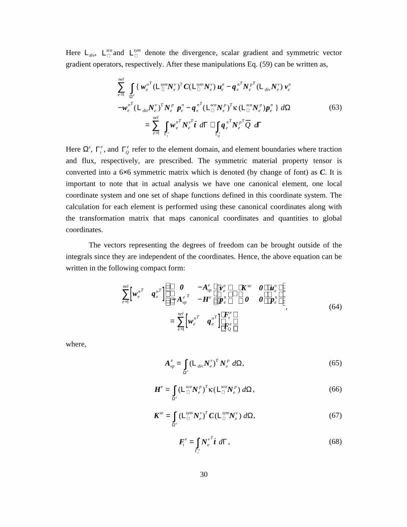
30

Here Ldiv, L∇sca and L∇

sym denote the divergence, scalar gradient and symmetric vector

gradient operators, respectively. After these manipulations Eq. (59) can be written as,

e =1

nel

∑ wenT

(L ∇symNe

v )T C(L∇symNe

v) uen

Ωe

∫ − q enT

NepT

(L div Nev) ve

n

−wenT

(L divNev )T Ne

p pen − q e

nT(L∇

scaNep )T (L∇

scaNep )pe

n dΩ

=e =1

nel

∑ w enT

NevT

t dΓΓt

e∫ + q e

nTNe

pTQ dΓ

ΓQe∫

(63)

Here Ωe, Γte , and ΓQ

e refer to the element domain, and element boundaries where traction

and flux, respectively, are prescribed. The symmetric material property tensor is

converted into a 6×6 symmetric matrix which is denoted (by change of font) as C. It is

important to note that in actual analysis we have one canonical element, one local

coordinate system and one set of shape functions defined in this coordinate system. The

calculation for each element is performed using these canonical coordinates along with

the transformation matrix that maps canonical coordinates and quantities to global

coordinates.

The vectors representing the degrees of freedom can be brought outside of the

integrals since they are independent of the coordinates. Hence, the above equation can be

written in the following compact form:

wenT

q enT[ ]

e =1

nel

∑0 −Avp

e

−Avpe T −He

ven

p en

+

K se 0

0 0

uen

pen

= wenT

q enT[ ] Ft

e

FQe

e =1

nel

∑, (64)

where,

Avpe = (L div Ne

v)T Nep dΩ

Ωe

∫ , (65)

He = (L ∇scaNe

p )T (L∇scaNe

p )Ωe

∫ dΩ , (66)

K se = (L∇symNe

v)T C(L∇symNe

v ) dΩΩe

∫ , (67)

Fte = Ne

v Tt dΓ

Γte

∫ , (68)

31

FQe = Ne

pQ dΓΓ Q

e

∫ . (69)

It is straightforward to assemble Eq. (64) into a global system where all vectors and

matrices are used to build their assembled counterpart according to standard finite

element assembly algorithms. The assembled matrices are defined by dropping the letter

‘e’ as a subscript or superscript. Since assembled w and q are arbitrary vectors, Eq. (64)

can be satisfied only if,

0 −Avp

−AvpT −H

vn

pn

+

K s 0

0 0

u n

0

=

Ft

FQ

, (70)

where all vectors and matrices are written in global form.

Equation (70) forms a first order differential-algebraic system to be solved in time

with a finite-difference method. There are alternative difference schemes that can be used

to solve such a system. A Crank-Nicholson scheme will be used, thus solid displacement

is given as,

uk +1n = vk +1

n + (1− )vkn( )∆t + uk

n , (71)

where the subscript refers to the time-step number, is a time-integration parameter and

t is the size of the time-step. As we see, displacement is calculated from a weighted

average of velocity at the next time-step (k+1) and the current one (k). For > 0.5, this

method is stable independent of the size of the time-step.

Substituting (71) into (70) and rearranging, results in,

∆tK s −Avp

−AvpT −H

vk +1n

p k +1n

=

Ft − K s (ukn + vk

n (1− )∆t)

FQ

. (72)

Equation (72) indicates that the system is solved for the first time step after the initial

conditions of the problem are imposed on the right hand side. The solution at current time

step (k) is used to update the right hand side for the solution of the next time step (k+1)

Note that the coefficient matrix does not change in this linear formulation unless t or

are chosen to vary.

32

4.5 Computer Implementation

4.5.1 Object Oriented Programming

Object-oriented programming (OOP) is a programming paradigm aimed at easy

extensibility and maintainability of large computer codes. An object-oriented simulation

models an application as a collection of objects. Each defined object models a specific

entity or event in an application problem and all objects work together to achieve the goal

and the task of the overall system. Objects can be compared to variables in traditional

programming languages but there is a significant difference. Unlike an object, a regular

variable captures only the data structure aspect of an object, not its behavior. In OOP,

each object is associated with certain data and functions [30].

Some programming languages are specifically designed for OOP, C++ being the

one in most widespread use. In C++, the object is called a class. Each class has a

collection of data that might include other class objects, and functions that perform tasks

related to the class and generally make use of the class data to do that. It is possible to

derive subtypes of objects that inherit the specified data and functions of the parent

object, but also possesses their own data and functions. The data and functions in each

object have different levels of accessibility from other objects including the parent and

child objects.

With that structure, running a finite element analysis code can be as simple as

invoking the “run” function of the “finite element analysis” class. This action then

invokes other actions which themselves activate other functions and make use of other

objects. The programmer can design a class structure that contain as many nested

processes as necessary.

The finite element formulations developed in this research are implemented

within Trellis [11], the object oriented finite element analysis framework of SCOREC,

and used to solve the problems described in the following chapters. Figure 5 displays the

symbols used to represent class objects, and indicates the derivation of a child class from

a parent class and the ownership of one class by the other. These symbols are utilized in

the class diagrams in the coming section.

33

Figure 5: Symbols used in object oriented diagrams.

4.5.2 Implementation of the Linear Analysis

Trellis is an object-oriented collection of software tools for general finite element

analysis [11]. It is written in the C++ programming language. The main libraries of

Trellis contain objects related to general finite element analysis, programming utilities,

mesh and model handling. The general finite element library includes all objects

corresponding to general and specific analyses, shape functions and mappings. Objects

related to data representation and storage, such as lists, are included in the programming

utilities library. The mesh library includes all mesh related objects such as elements,

faces, vertices or usages. The model library not only includes model related objects but

also has interfaces to different commercial solid modeler packages such as Parasolid

used in the current work. Other software packages such as the PETSc matrix algebra

package are also interfaced to Trellis in a convenient manner.

Our formulation is implemented as a separate library within this framework. For

routine finite element operations such as numerical integration, assembly or linear system

solving basic libraries of Trellis are utilized. A complete description of Trellis is beyond

the scope of this work; only those major object hierarchies related to the current

implementation are described here.

One major object is the analysis object which is a high level class called

FEAnalysis for general finite element analysis from which different types of finite

element analyses objects such as ElasticityAnalysis or

HeatTransferAnalysis are derived. FEAnalysis also owns a class called

class_functions()

ClassObjectName class object

derivation

ownership

34

FEAnalysis

HeatTransferAnalysis ElasticityAnalysis

VPBiphasicAnalysis

AttCase

parse_bc()

bc_vp_specific()

...

BiphasicAnalysis

make_vp_element()

......

...

Figure 6: Analysis hierarchy of the implemented finite element code.

AttCase that handles the necessary attribute information for the problem under analysis

(Fig. 6). The parent object performs some general tasks, such as handling the mesh and

the model, while the child classes are assigned tasks specific to a certain analysis like

taking the necessary steps to set up the stiffness matrix for the problem. We have a

BiphasicAnalysis object which is derived from FEAnalysis. All the relevant

data, such as fields and boundary conditions for a biphasic analysis are defined (but not

implemented) in this class. This class parses the boundary conditions by invoking the

necessary functions in the child classes. The VPBiphasicAnalysis class is derived

from BiphasicAnalysis and implements the necessary functions defined there

according to the v-p formulation described in this chapter. It creates the element object

and boundary condition objects of the v-p formulation (note that the same physical

boundary condition might have a different mathematical form in different finite element

formulations). Other finite element formulations of the soft tissue problem will require

different classes derived from BiphasicAnalysis.

Another important class is StiffnessContributor which is a parent class

for many objects that contribute to the coefficient matrix of the final linear system, such

as element matrices or essential boundary conditions. The BiphasicElement3D class

that implements some element aspects that are common to different finite element

formulation of the soft tissue problem is derived from this class. For example the solid

stiffness term, Eq. (67), is known to be the same in all known formulations and hence can

be created in this generic object (it can be always re-implemented in the child class when

necessary). The functions that calculate element matrices specific to the v-p formulation

35

StiffnessContributor

HeatTransferSC3D

BiphasicElm_VP3D

solid_stiffness_term()

vp_stiffness_terms()

BiphasicElement3D

...

...

Figure 7: Element hierarchy of the implemented finite element code.

are members of BiphasicElm_VP3D class which is a child of

BiphasicElement3D (Fig. 7).

VPTrapezoidalTI class handles the trapezoidal time integration and controls

the time-stepping using velocity and displacement. It owns a class VPTrapTIAssm that

processes and assembles the system contributors, namely element matrices and force

vectors, according to the trapezoidal time integration rule. It also updates the system at

each time step as prescribed by the v-p formulation and trapezoidal rule (Fig. 8). Other

integration rules will require that new classes be implemented.

TimeIntegrator LinearSystemAssembler

VPTrapTIAssmtime_stepping()

...

VPTrapezoidalTI

...

process_SC()update_system()

Figure 8: Time integrator and system assembler hierarchy of the implemented finite

element code.

36

Another important class used in the implementation is VPFaceTraction,

which is derived from ForceContributor class and calculates the force vector

terms (i.e. contributes to the force vector of the final linear system).

The material property information in our analysis is maintained by the

BiphasicMaterial class, which owns an elastic solid phase object (the

ElasMat3dDispForm class) such as LinearIsotropicElasticMaterial or

TransverslyIsotropicElasticMaterial as member data. The properties that

are unique to a biphasic material, such as permeability or the volume fraction of the

phases, are handled by BiphasicMaterial. The actions related to the solid phase,

such as returning the stiffness matrix or calculating the stress, are functions in the solid

phase classes. In that sense the BiphasicMaterial class provides access to the solid

phase (Fig. 9).

TransverslyIsotropicElasticMaterialLinearIsotropicElasticMaterial

ElasMat3dDispForm

permeability()

BiphasicMaterial...

volume_fraction()

return_stiffness()calculate_stress()


Figure 9: Material hierarchy of the implemented finite element code.

4.6 Nonlinear Formulation

In many physiological cases cartilage undergoes large deformations such that an

infinitesimal strain analysis is not adequate to describe its in vivo mechanical behavior. In

this section, the analysis described previously in this chapter is extended to take

geometric and material nonlinearities into account. In this work, as is common in solid

mechanics problems, a Lagrangian description is used to follow motion of the material

points of the body.

As pointed out earlier, the weak form of our problem, Eq. (56), is derived in a

general way such that it is valid for geometric and/or material nonlinearities. In nonlinear

analysis, however, the problem domain Ω and boundary Γ are no longer fixed. They are

37

likely to change shape and size with deformation and the integrals need to be evaluated

accordingly. Keeping the deformed integration domains in Eq. (56) results to the so-

called updated Lagrangian formulation where the problem domain needs to be “updated”

as motion occurs. An alternative to the updated Lagrangian formulation is the total

Lagrangian formulation where all quantities are “pushed back” to the initial

configuration, i.e. expressed in a material coordinate system [10].

In the finite element method, interpolation functions for each element are formed

using the coordinates of the nodes in the element. Hence, the difference between spatial

and initial derivative quantities is dependent on whether deformed or initial nodal

coordinates are used in those interpolations. Depending on the structure of the computer

program used, one way can be easier than the other. A mixed approach where some

quantities are expressed in spatial configuration and others in the initial configuration is

also possible [1]. In this thesis the total Lagrangian approach is used. One reason for that

was that the resulting analysis was implemented in an object-oriented framework. An

updated Lagrangian approach would necessitate that nodal coordinates be updated every

time step, and potentially every iteration, depending on the nonlinear solver chosen.

Although it is possible to update the mesh when necessary, this operation complicates the

computer implementation and undermines object-oriented paradigm.

A total Lagrangian form of the problem can be obtained when Eq. (56) is

rewritten such that its differentiation operations and integral domains are expressed with

respect to the initial configuration using F and Eq. (21). In that case, after substituting

Eq. (40), (56) takes the following form:

t r [ 2 (∇0w)T FΨC

]− q(F−T :∇0v)J − p(F−T :∇0w)JΩ0

∫

− (F−T∇0 p) • (F−T∇0q)J dΩ0 = w • t 0 JΓdΓ0

Γt0

∫ + qQ J ΓdΓ0

ΓQ 0

∫(73)

Here, ∇0 denotes the gradient operator with respect to the initial configuration and is

related to ∇ through components of F-1. The ratio of the current area to the initial area,

JΓ, can be found by taking the dot product of Eq. (22) with itself to give

JΓ = J n0TC−1n0 , (74)

where n0 is the reference surface normal. It should be noted that the prescribed traction t 0is expressed in the initial configuration. The first term in Eq. (73) is the solid phase

nonlinearity and will be denoted by Gs , i.e:

38

G s = tr[(∇0w)T FS E ] dΩ0Ω0

∫ . (75)

Gs is the dominant nonlinear term in Eq. (73) representing the material nonlinearity in the

problem. In the remaining terms, F and J, which are functions of the motion are

multiplied in various combinations creating geometric nonlinearities. These terms take

into account the changing shape and size of the problem domain when evaluating

derivatives and integrating.

4.6.1 Linearization

A nonlinear equation such as Eq. (73) is solved through an iterative technique

where consecutive contribution are made to an initial guess at each iteration until

convergence occurs. In general, given a system of nonlinear equations r(u)

r (u) = 0, (76)

to be solved for u, the corresponding Newton-Raphson procedure creates at each iteration

a linear system like

∂r (u)∂u ˜ u

u = Dr( ˜ u )[ u] = r = −r( ˜ u ), (77)

where ˜ u denotes the current state of the solution variables and u is the variation from

the current state. In practice, in a Newton-Raphson iteration scheme ˜ u is the solution

estimated from the previous iteration and u is the correction proposed to it. In the rest of

this chapter, the notation DT( ˜ u )[ u], or T in short, will denote the change in the tensor

T at the current deformation state ˜ u along the direction u (i.e. its directional derivative).

Applying the linearization as demonstrated in Eq. (77) to all terms in (73) is a

fairly straightforward procedure and results in the following expression for the fully

linearized form of our nonlinear system:

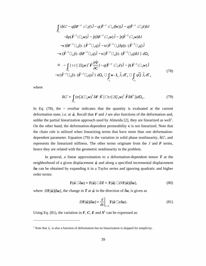
39

Gs − q( F−T :∇0 ˜ v ) ˜ J − q( ˜ F −T :∇0 ( v)) ˜ J Ω0

∫ − q( ˜ F −T :∇0 ˜ v ) J

− p( ˜ F −T:∇0w) ˜ J − ˜ p ( F−T:∇0w) ˜ J − ˜ p ( ˜ F −T:∇0w) J

− ( F−T∇0˜ p ) • ( ˜ F −T∇0q) ˜ J − ( ˜ F −T∇0( p)) • ( ˜ F −T∇0q) ˜ J

− ( ˜ F −T∇0˜ p ) • ( F−T∇0q) ˜ J − ( ˜ F −T∇0

˜ p ) • ( ˜ F −T∇0q) J dΩ0

= − t r [ 2 (∇0w)T ˜ F ˜ Ψ C

] − q( ˜ F −T :∇0 ˜ v ) ˜ J − ˜ p ( ˜ F −T:∇0w) ˜ J Ω0

∫− ( ˜ F −T∇0

˜ p ) • ( ˜ F −T∇0q) ˜ J dΩ0 + w • t 0˜ J ΓdΓ0

Γ t0

∫ + qQ ˜ J ΓdΓ0

ΓQ0

∫(78)

where

Gs = (tr[2(∇0w)T F SE ] + t r [ 2 (∇0w)T ˜ F SE ]Ω0

∫ )dΩ0 . (79)

In Eq. (78), the ~ overbar indicates that the quantity is evaluated at the current

deformation state, i.e. at ˜ u . Recall that F and J are also functions of the deformation and,

unlike the partial linearization approach used by Almeida [2], they are linearized as well1.

On the other hand, the deformation-dependent permeability is not linearized. Note that

the chain rule is utilized when linearizing terms that have more than one deformation-

dependent parameter. Equation (79) is the variation in solid phase nonlinearity, Gs, and

represents the linearized stiffness. The other terms originate from the J and F terms,

hence they are related with the geometric nonlinearity in the problem.

In general, a linear approximation to a deformation-dependent tensor T at the

neighborhood of a given displacement ˜ u and along a specified incremental displacement

u can be obtained by expanding it in a Taylor series and ignoring quadratic and higher

order terms:

T( ˜ u + u) ≈ T( ˜ u ) + T = T( ˜ u ) + DT( ˜ u )[ u], (80)

where DT( ˜ u )[ u], the change in T at ˜ u in the direction of u, is given as

DT( ˜ u )[ u] =d

d = 0

T( ˜ u + u) . (81)

Using Eq. (81), the variation in F, C, E and SE can be expressed as:

1 Note that JΓ is also a function of deformation but its linearization is skipped for simplicity.

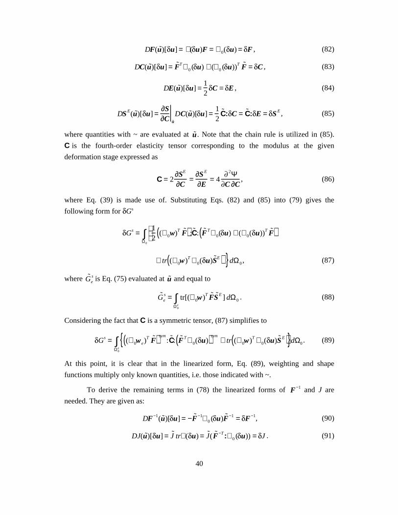
40

DF( ˜ u )[ u] = ∇( u)F = ∇0( u) = F , (82)

DC( ˜ u )[ u] = ˜ F T∇0 ( u) + (∇0 ( u))T ˜ F = C , (83)

DE( ˜ u )[ u] =12

C = E , (84)

DS E( ˜ u )[ u] =∂S∂C ˜ u

DC( ˜ u )[ u] =12

˜ C : C = ˜ C : E = S E , (85)

where quantities with ~ are evaluated at ˜ u . Note that the chain rule is utilized in (85).

C is the fourth-order elasticity tensor corresponding to the modulus at the given

deformation stage expressed as

C = 2∂SE

∂C=

∂S E

∂E= 4

2ΨC ∂C

, (86)

where Eq. (39) is made use of. Substituting Eqs. (82) and (85) into (79) gives the

following form for Gs

Gs =12

(∇0w)T ˜ F ( ) : ˜ C : ˜ F T∇0( u) + (∇0( u))T ˜ F ( ) Ω0

∫

+ tr (∇0w)T ∇0( u) ˜ S E( ) dΩ0 , (87)

where ˜ G es is Eq. (75) evaluated at ˜ u and equal to

˜ G es = tr[(∇0w)T ˜ F ˜ S E ] dΩ0

Ω0e

∫ . (88)

Considering the fact that C is a symmetric tensor, (87) simplifies to

Gs = (∇0w e)T ˜ F ( ) sym

: ˜ C : ˜ F T∇0( u)( )sym+ tr (∇0w)T ∇0( u) ˜ S E( )

Ω0e

∫ dΩ0 . (89)

At this point, it is clear that in the linearized form, Eq. (89), weighting and shape

functions multiply only known quantities, i.e. those indicated with ~.

To derive the remaining terms in (78) the linearized forms of F−1 and J are

needed. They are given as:

DF−1( ˜ u )[ u] = − ˜ F −1∇0 ( u) ˜ F −1 = F−1, (90)

DJ( ˜ u )[ u] = ˜ J tr∇( u) = ˜ J ( ˜ F −T:∇0 ( u)) = J . (91)

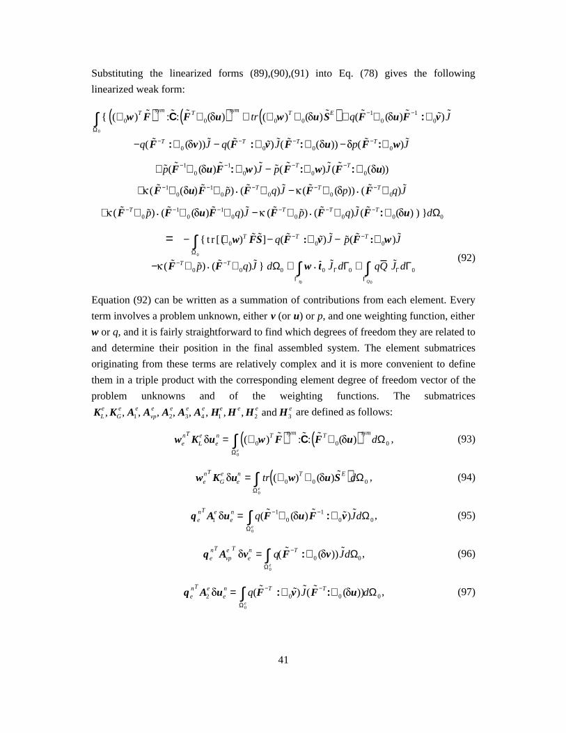
41

Substituting the linearized forms (89),(90),(91) into Eq. (78) gives the following

linearized weak form:

(∇0w)T ˜ F ( )sym: ˜ C : ˜ F T∇0( u)( ) sym

+ tr (∇0w)T ∇0( u) ˜ S E( ) + q( ˜ F −1∇0 ( u) ˜ F −1 :∇0˜ v ) ˜ J

Ω0

∫−q( ˜ F −T :∇0 ( v)) ˜ J − q( ˜ F −T :∇0 ˜ v ) ˜ J ( ˜ F −T:∇0( u)) − p( ˜ F −T:∇0w) ˜ J

+ ˜ p ( ˜ F −1∇0 ( u) ˜ F −1:∇0w) ˜ J − ˜ p ( ˜ F −T:∇0w) ˜ J ( ˜ F −T:∇0( u))

+ ( ˜ F −1∇0( u) ˜ F −1∇0 ˜ p ) • ( ˜ F −T∇0q) ˜ J − ( ˜ F −T∇0 ( p)) • ( ˜ F −T∇0q) ˜ J

+ ( ˜ F −T∇0 ˜ p ) • ( ˜ F −1∇0 ( u) ˜ F −1∇0q) ˜ J − ( ˜ F −T∇0 ˜ p ) • ( ˜ F −T∇0q) ˜ J ( ˜ F −T:∇0( u) ) dΩ0

= − t r [ (∇0w)T ˜ F S ]− q( ˜ F −T :∇0 ˜ v ) ˜ J − ˜ p ( ˜ F −T :∇0w) ˜ J Ω0

∫− ( ˜ F −T∇0 ˜ p ) • ( ˜ F −T∇0q) ˜ J dΩ0 + w • t 0 ˜ J ΓdΓ0

Γ t0

∫ + qQ ˜ J ΓdΓ0

ΓQ0

∫(92)

Equation (92) can be written as a summation of contributions from each element. Every

term involves a problem unknown, either v (or u) or p, and one weighting function, either

w or q, and it is fairly straightforward to find which degrees of freedom they are related to

and determine their position in the final assembled system. The element submatrices

originating from these terms are relatively complex and it is more convenient to define

them in a triple product with the corresponding element degree of freedom vector of the

problem unknowns and of the weighting functions. The submatrices

KLe, KG

e, A1e, Avp

e , A2e, A3

e, A4e, H1

e, H e, H2e and H3

e are defined as follows:

wenT

KLe ue

n = (∇0w)T ˜ F ( )sym: ˜ C : ˜ F T∇0( u)( ) sym

dΩ0

Ω0e

∫ , (93)

wenT

KGe ue

n = tr (∇0w)T ∇0 ( u) ˜ S E( )dΩ0

Ω0e

∫ , (94)

q enT

A1e ue

n = q( ˜ F −1∇0 ( u) ˜ F −1 :∇0˜ v ) ˜ J

Ω0e

∫ dΩ0 , (95)

q enT

Avpe T

ven = q( ˜ F −T :∇0 ( v)) ˜ J

Ω0e

∫ dΩ0 , (96)

q enT

A2e ue

n = q( ˜ F −T :∇0˜ v ) ˜ J ( ˜ F −T:∇0 ( u))

Ω0e

∫ dΩ0 , (97)

42

wenT

A3e ue

n = ˜ p ( ˜ F −1∇0 ( u) ˜ F −1:∇0w) ˜ J Ω0

e

∫ dΩ0 , (98)

wenT

A4e ue

n = ˜ p ( ˜ F −T:∇0w) ˜ J ( ˜ F −T:∇0 ( u))dΩ0

Ω0e

∫ , (99)

q enT

H1e ue

n = ( ˜ F −1∇0 ( u) ˜ F −1∇0˜ p ) • ( ˜ F −T∇0q) ˜ J dΩ0

Ω0e

∫ , (100)

q enT

H e pen = ( ˜ F −T∇0( pe)) • ( ˜ F −T∇0qe)

˜ J dΩ0

Ω0e

∫ , (101)

q enT

H2e ue

n = ( ˜ F −T∇0˜ p ) • ( ˜ F −1∇0( u) ˜ F −1∇0q) ˜ J dΩ

Ω0e

∫ , (102)

q enT

H3e ue

n = ( ˜ F −T∇0˜ p ) • ( ˜ F −T∇0q) ˜ J ( ˜ F −T:∇0( u))dΩ0

Ω0e

∫ . (103)

The KLe and KG

e element matrices are often encountered in nonlinear elasticity and called

the large deformation stiffness matrix and geometric stiffness matrix, respectively.

Substituting Eqs. (93) through (103) in the weak form, (92), gives the following

linear first order system:

wenT

q enT[ ] 0 −Avp

e

−Avpe T

−He

ven

p en

+

M e 0

De 0

uen

0

e =1

nel

∑

= w enT

q enT[ ]

e =1

nel

∑Ft

e

FQe

−K se ˜ u e

n

0

+

Avpe ˜ p e

n

Avpe T

˜ v en + H e ˜ p e

n

(104)

where

Me = KLe + KG

e + A3e − A4

e, (105)

De = A1e − A2

e + H1e + H2

e − H3e , (106)

K se = KLe + KG

e . (107)

As the next step all the known quantities are moved to the right hand side and assembly is

performed such that all matrices and vectors are replaced with their global counter parts.

Since the weighting functions are arbitrary, Eq. (104) constitutes a solvable linear system

that is expressed as:

43

0 −Avp

−AvpT −H

v n

pn

+

M 0

D 0

un

0

=

Ft

FQ

−

K s ˜ u n

0

+

Avp ˜ p n

AvpT ˜ v sn + B˜ p n

. (108)

Equation (108) is a first order differential-algebraic system due to the presence of

velocity v and displacement u as unknowns. It can be solved for the unknown increments

v, p and u in order to update the current solution estimates ˜ v , ˜ p , and ˜ u . The right hand

side of Eq. (108) is the problem residual and should slowly vanish as convergence occurs

through the iterative process.

4.6.2 Partial Linearization

When solving Eq. (76), any procedure that causes successive reductions in the

residual at each iteration is an acceptable scheme. In other words, there is no unique

“convergence path” leading to the solution. This fact is utilized by calculating an

approximate tangent matrix (left hand side of Eq. (77)) rather than an exact one. In

biphasic tissue problems, it is common to approximate the tangent matrix by taking the

Gs term as the only nonlinearity present and ignoring the geometric nonlinearities [2, 67,

98]. The same approach, when applied to Eq. (73) causes the matrices

A1e, A2

e, A3e, A4

e, H1e, H2

e and H3e to vanish, simplifying Eq. (104) to

wenT

q enT[ ] 0 −Avp

e

−Avpe T

−He

˜ v en

˜ p en

+

K se 0

0 0

uen

0

e =1

nel

∑

= w enT

q enT[ ]

e =1

nel

∑Ft

e

FQe

−K se ˜ u e

n

0

+

Avpe ˜ p e

n

Avpe T

˜ v en + He ˜ p e

n

(109)

The partially linearized form given in Eq. (109) is encountered often, so it is proper to

show the corresponding element matrices in operator notation as done in the linear

formulation. First, we define the following operators:

L0∇sca =

∂∂X∂

∂Y∂

∂Z

L0div =

L0∇sca 0 0

0 L0∇sca 0

0 0 L 0∇sca

0 =0

0

0

(110)

Using the above linear operators, element matrices and vectors in Eq. (109) are given as:

Avpe = (FINV L 0

div Nev)T Ne

p J dΩ0

Ω0e

∫ , (111)

44

He = (F -T L 0∇sca Ne

p )T (F−TL 0∇scaNe

p )Ω0

e

∫ J dΩ0 , (112)

Fte = Ne

v• t 0 JΓdΓ0

Γ0 te

∫ , (113)

FQe = Ne

pQ J ΓdΓ0

Γ0Qe

∫ . (114)

The matrix FINV is composed of the entries of F−1 and defined in the Appendix B.

Similarly, KLe and KG

e , defined in Eqs. (93) and (94), can be rewritten separate from the

multiplying degree of freedom vectors using the same operators:

KLe = (FL L 0

div Nev)T ˜ C (FL

Ω0e

∫ L 0div Ne

v) dΩ0 , (115)

KGe = (L 0

div Nev)T SG

E (Ω0

e

∫ L 0div Ne

v) dΩ0 . (116)

In the above equations, ˜ C , as in the linear analysis, is the matrix representing the fourth-

order tensor C. FL is a matrix composed of the entries of F and are given in Appendix B.

SGs is defined as

SGE =

S E 0 0

0 S E 0

0 0 S E

. (117)

After assembly, the corresponding global system becomes:

0 −Avp

−AvpT −H

v n

pn

+

K s 0

0 0

un

0

=

Ft

FQ

−

K s ˜ u n

0

+

Avp ˜ p n

AvpT ˜ v sn + B˜ p n

. (118)

Note that the right hand side of the above equation is still equivalent to the residual.

Unlike the fully linearized form, Eq. (104), the above system is symmetric and requires

that fewer terms be computed; this makes it computationally desirable. On the other

hand, depending on the problem at hand, this form might take a higher number of

iterations to converge due to inexactness of the tangent matrix.

Equations (108) and (118) representing, respectively, fully linearized and

minimally linearized forms of the weak form, and are two extremes in complexity when

solving the nonlinear soft tissue problem. It is possible to choose an intermediate method

by selectively linearizing terms other than Gs. The nonlinear penetration problem is a

45

challenging numerical problem and thus different intermediate linearizations were

attempted to increase numerical efficiency. One efficient way is to linearize the F terms

while ignoring the nonlinearity associated with J. In that case, the final system has the

following simplified forms for M and D.

Me = KLe + KG

e + A3e, (119)

De = A1e + H1

e + H2e. (120)

The final linear equation system can be written in a simple notation as:

Y v + K u = f , (121)

where

Y =0 −Avp

−AvpT −H

K =

M 0

D 0

v =

vn

pn

u =

u n

0

f =Ft

FQ

−

K s ˜ u n

0

+

Avp˜ p n

AvpT ˜ v n + B˜ p n

(122)

4.6.3 Solution of the Nonlinear System

As in the linear analysis, the relation between velocity and displacement is

established using the Crank-Nicholson rule according to Eq. (71). Before going into the

details of this scheme it is worthwhile to briefly describe other methods to solve

differential algebraic systems.

It is possible to treat methods to solve differential algebraic systems or ordinary

differential equations, in general, in two categories: one-step and multi-step methods.

Each group includes explicit and implicit methods. Using ordinary differential equation

notation, a first order system can be expressed as:

y = f (y) y(0) = y0 . (123)

For the above system, explicit one-step, explicit multi-step, implicit one-step and implicit

multi-step methods are given, respectively, as:

yk +1 = P(yk )

yk +1 = P(yk, yk −1,K,yk − l)

yk +1 = P(yk +1, yk )

yk +1 = P(yk +1, yk,K,yk − l)

(124)

where P indicates a function describing the numerical procedure

46

Explicit one-step methods are not used since they are known to be unstable.

Multi-step methods, both implicit and explicit, require evaluation of the stiffness matrix

at more than one past time steps. This will require storing of the solution at as many

previous time steps as the order of the method prescribes. Furthermore, the method can

be applied only after this number of time steps has been taken with another method

(usually a one-step method) that gives the “initial condition” for the multi-step method. A

multi-step method is relatively complex but can lead to increased accuracy. The

efficiency of such a scheme from a computational point of view poses an important

research question; however, it is beyond the scope of this thesis.

To solve our differential algebraic system, an implicit one-step method is the

simplest option providing reasonable accuracy. As a result, a Crank-Nicholson rule was

chosen, where the integration parameter is modified according to the nature of the

problem at hand (i.e. considering the type of boundary conditions, and geometry of the

problem domain) to ensure stability.

It is possible to use a higher-order implicit time integration method for time

stepping such as an implicit Runge-Kutta method [17, 37]. In this method the parameters

required for time stepping are unknown and need be determined as part of the solution

process. This approach was not studied.

In Eq. (121), the problem unknowns are the increments of the problem variables,

unlike in linear analysis where the unknowns are the variables themselves. At each time

step the system should be repeatedly solved until convergence occurs. Then the solution

is updated to form an initial guess for the next time step and the iteration is repeated until

convergence is again achieved. The variations in the solution variables, v and u, are

defined with respect to the time integration scheme as:

vk +1(i ) = vk +1

( i) − vk +1( i −1)

uk +1(i ) = uk +1

( i) − uk +1( i −1)

(125)

where the superscript denotes the iteration number and the subscript, as in the linear

analysis, indicates the time step. Using (71) and noting that the variation of un and vn, the

converged solutions from the previous time step, is zero, gives the relation between u

and v as

uk +1(i ) = ∆t vk +1

( i ) . (126)

Substituting Eq. (126) into Eq. (121) and rearranging gives

47

(Yk +1( i −1) + ∆t Kk +1

( i−1)) vk +1( i) = f k +1

( i−1), (127)

where subscripts and superscripts have been added to the matrices to indicate the time

step and iteration number, respectively, of the deformation state at which they are

formed.

In a full Newton-Raphson method, Eq. (127) is solved and the solution is updated

using

vk +1( i) = vk +1

( i −1) + vk +1( i)

uk +1( i) = uk +1

( i −1) + uk +1( i) = uk +1

( i −1) + ∆t vk +1(i )

(128)

The right-hand side and left-hand side of Eq. (127) are updated by reevaluating Y, K and f

at the new approximation to give the new system of equations. This procedure is repeated

until convergence occurs. Convergence is checked by observing a suitable norm of f

which should decrease since it indicates the magnitude of the residual of the problem.

In an effort to increase the numerical efficiency in the nonlinear penetration

problem, a u-p formulation has also been studied. That requires un to be retained in the

problem. In this case, using Eq. (126), vn is eliminated, and u and p (rather than v and p)

become the main problem variables. It is easy to show that this closely-related

formulation gives the following final system of equations:

(Yk +1( i −1) + Kk +1

( i−1)) uk +1( i) = f k +1

( i−1), (129)

where

Yk +1(i −1) =

0 −Avp

−1

∆tAvp

T −H

k +1

( i−1)

uk +1( i−1) =

u n

pn

k +1

( i−1)

. (130)

In the above equation, the indices attached to the brackets indicate the time step and

iteration at which the corresponding matrix and vector are evaluated. The K and f terms

have the same form as in the v-p formulation. Note the vector u contains degrees of

freedom for both main problem variables, u and p.

A full Newton-Raphson method requires the full linear system to be updated and

solved at every iteration. This is computationally expensive and thus more efficient

approaches are taken. In quasi-Newton methods, the tangent-stiffness matrix (or its

inverse) is approximated without performing a linearization and updated whenever

necessary at each iteration. The various quasi-Newton algorithms, such as Secant,

48

Broyden or Broyden-Fletcher-Goldfarb-Shanno (BFGS) methods, differ only by the

choice of the matrix updating formula [49].

In the modified Newton method, only the right hand side of the system, namely

the problem residual f, is updated after every iteration. In this approach, Eq. (127)

becomes

(Yk +1(0) + ∆t K k +1

(0) ) vk +1( i) = fk +1

( i −1). (131)

Updating f insures that the residual is evaluated at every iteration. As long as the residual

gradually decreases and vanishes at the end of iterations, the analyst is free to choose if or

when to update the left hand side of Eq.(131). As mentioned earlier in this chapter, there

is no unique “path” to a converged solution in an iterative technique. With respect to

Eq. (127), any updating procedure that will reduce the norm of f properly will lead

eventually to a converged solution. In this work, the modified Newton scheme is adopted;

the numerical solution procedure is outlined on Table 1.

Table 1: The numerical procedure for the nonlinear problem

Iteration at timestep n+1:

1) If it is the first iteration within that time step, namely i = 0, obtain the estimates for v

and u vector from the converged values of the previous time step :

vn+1(0) = vn un+1

(0) = un + ∆tvn

2) Do the following until | v| is sufficiently small indicating convergence

a) Solve the system to find the increment

(Yn +1(0) + ∆t Kn+1

(0) ) vn +1( i ) = fn +1

( i −1)

b) If necessary do a line search to find β , otherwise set β = 1.0

vn+1( i) = vn+1

( i−1) + vn+1( i) un+1

( i) = un+1( i−1) + ∆t vn +1

( i )

c) Update the right hand side only, or potentially the whole system depending

on the convergence behavior. Update the iterate counter to i+1

3) Go to the next time step

49

4.6.4 Line Search

The performance of a solution procedure depends not only on the finite element

formulation used but also on the type of problem (i.e. geometry of the problem domain,

boundary conditions etc.) to be solved. In many cases, the Newton iteration does not

converge when strong nonlinearities are present in the problem. Such is the case for the

example problems presented in Chapter 7. As an additional precaution to insure

convergence, a line search algorithm was incorporated with the modified Newton solver.

The line search technique is often utilized in unconstrained optimization and can

be used with a wide range of iterative solution methods [21]. In line search, instead of

updating the approximation to the solution at each iteration by the full correcting

increment, the correcting increment is multiplied by a scaling factor . The scaling factor

is determined such that the scaled increment gives a better approximation to the solution

than the full increment. The usual strategy is to define an objective function Φ( ) and

choose in such a way that this function fulfills a specified condition. It is possible to

select a function that vanishes when is optimal. In other words, the condition that the

line search should fulfill is

Φ(v i + v i) = 0 . (132)

This approach is computationally expensive since Φ has to be evaluated several times

until Eq. (132) is satisfied [49]. What is usually done in practice is to set a condition on

Φ( ) such that it is monotonically and sufficiently reduced from one iteration to the next.

This can be expressed as

Φ(v i + v i) < Φ(v i), (133)

where 0 < < 1.0 is a scalar that is problem-dependent and chosen heuristically. Several

objective functions have been proposed in the literature to determine the scaling factor

[32]. In our research, as our objective function we picked the magnitude of the residual

and tried to fulfill

f i+1 < f i , (134)

where the bars denote the magnitude of the vector.

In our implementaton, if the modified Newton iteration fulfills (134), the line

search procedure is skipped. Otherwise, is reduced starting from a specified value, 0,

with a specified increment . If reducing increases the magnitude of the residual, then

50

is increased with the same increment. The solution estimates are updated using the

optimal accordingly as

vk +1( i+1) = vk +1

( i ) + vk +1( i)

uk +1( i+1) = uk +1

( i ) + uk +1( i)

(135)

The residual f is reevaluated with the above estimates. This procedure is repeated until

Eq. (134) is satisfied. If none of the values within the specified range fulfills this

condition, a full-Newton update is performed by reevaluating Y, K and f , and the system

is solved again. In our tests, this procedure has proven to be effective for a wide variety

of problem configurations. However, the “correct” 0 and differ from one problem to

the other and their choice is critical to the efficiency of the algorithm. For example, a 0

that is too low might lead to excessive full-Newton updates, or a too small might

necessitate excessive residual evaluations, either of which reduces the computational

efficiency. On the other hand, some computational inefficiency might be risked to ensure

convergence.

4.7 Computer Implementation of the Nonlinear Analysis

The general structure of Trellis has been described earlier. The general

capabilities for implementing a nonlinear finite element analysis exist in Trellis and have

been used for elasticity problems. However, the time-dependent nature of our problem

required some general finite element objects to be programmed beyond those specific to

nonlinear biphasic analysis.

The first object necessary to implement the nonlinear biphasic problem is a

corresponding analysis class which is called NonlinVPBiphasicAnalysis and is

derived from VPBiphasicAnalysis. The NonlinVPBiphasicAnalysis class

specializes the function of VPBiphasicAnalysis that invokes the calculation of the

element matrix object. Also, the traction boundary condition, which has a different form

in nonlinear analysis, is calculated by invoking a different function (Fig. 10). The element

matrix object for the nonlinear analysis is called BiphasicElm_NonlinVP3D, and is

a child of BiphasicElm_VP3D class. The BiphasicElm_NonlinVP3D class re-

implements the functions that calculate the element matrices since they are

mathematically different in nonlinear analysis (Fig. 11).

Similarly, the force vector, which is different in nonlinear analysis, is calculated

using a new class, called VPFaceTractionLD, that takes large deformation into

account.

51

FEAnalysis

HeatTransferAnalysis ElasticityAnalysis

VPBiphasicAnalysis

AttCase

parse_bc()

bc_vp_specific()

...

BiphasicAnalysis

make_vp_element()

......

...

Nonlin_VPBiphasicAnalysis

make_nonlin_vp_element()nonlin_traction_bc()

Figure 10: Nonlinear analysis object in the analysis hierarchy.

StiffnessContributor

HeatTransferSC3D

BiphasicElm_VP3D

solid_stiffness_term()

vp_stiffness_terms()

BiphasicElement3D

...

...

BiphasicElm_NonlinVP3D

nonlin_vp_stiffness_terms()

Figure 11: Nonlinear biphasic stiffness object in the stiffness contributor hierarchy.

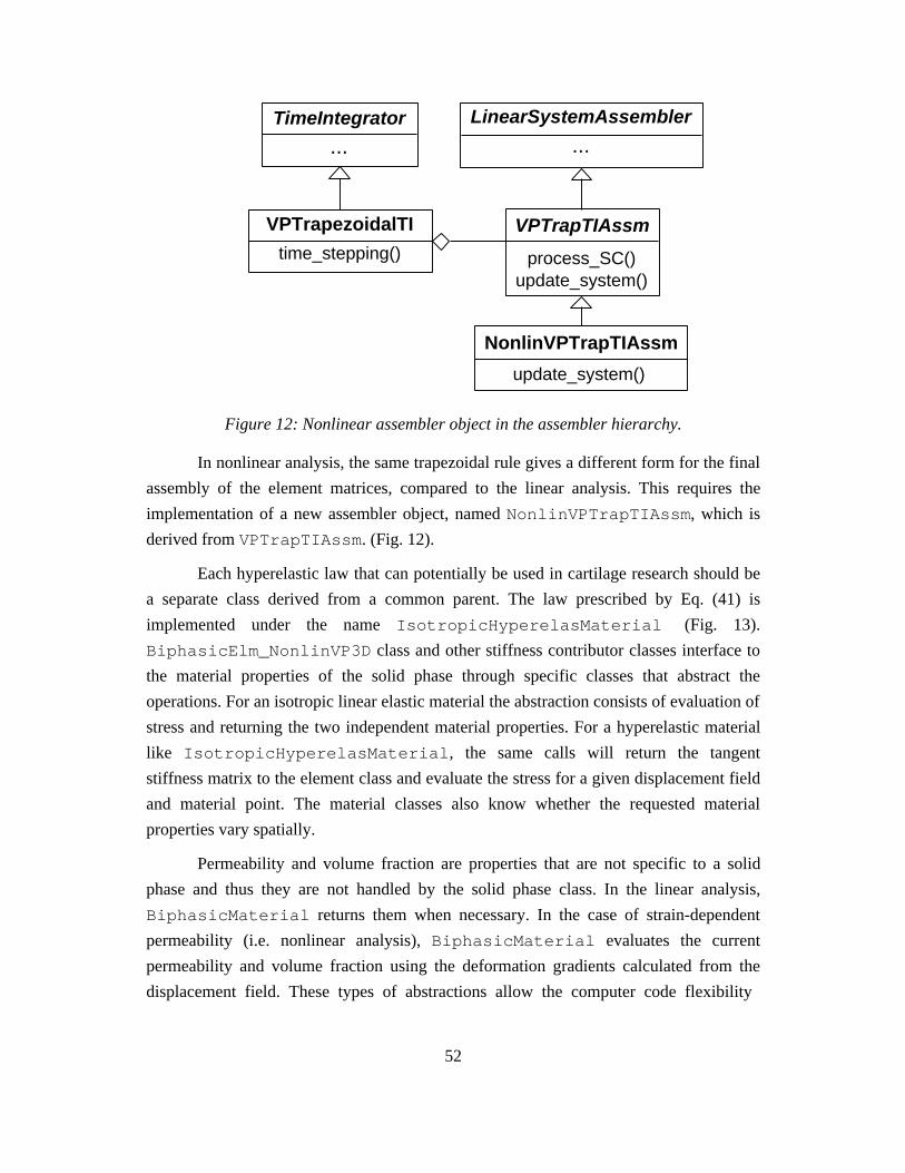
52

TimeIntegrator LinearSystemAssembler

VPTrapTIAssm

time_stepping()

...

VPTrapezoidalTI

...

process_SC()update_system()

NonlinVPTrapTIAssm

update_system()

Figure 12: Nonlinear assembler object in the assembler hierarchy.

In nonlinear analysis, the same trapezoidal rule gives a different form for the final

assembly of the element matrices, compared to the linear analysis. This requires the

implementation of a new assembler object, named NonlinVPTrapTIAssm, which is

derived from VPTrapTIAssm. (Fig. 12).

Each hyperelastic law that can potentially be used in cartilage research should be

a separate class derived from a common parent. The law prescribed by Eq. (41) is

implemented under the name IsotropicHyperelasMaterial (Fig. 13).

BiphasicElm_NonlinVP3D class and other stiffness contributor classes interface to

the material properties of the solid phase through specific classes that abstract the

operations. For an isotropic linear elastic material the abstraction consists of evaluation of

stress and returning the two independent material properties. For a hyperelastic material

like IsotropicHyperelasMaterial, the same calls will return the tangent

stiffness matrix to the element class and evaluate the stress for a given displacement field

and material point. The material classes also know whether the requested material

properties vary spatially.

Permeability and volume fraction are properties that are not specific to a solid

phase and thus they are not handled by the solid phase class. In the linear analysis,

BiphasicMaterial returns them when necessary. In the case of strain-dependent

permeability (i.e. nonlinear analysis), BiphasicMaterial evaluates the current

permeability and volume fraction using the deformation gradients calculated from the

displacement field. These types of abstractions allow the computer code flexibility

53

TransverslyIsotropicElasticMaterialLinearIsotropicElasticMaterial

ElasMat3dDispForm

permeability()

BiphasicMaterial...

volume_fraction()



IsotropicHyperelasMaterial


Figure 13: Nonlinear biphasic stiffness object in the stiffness contributor hierarchy.

characteristic of OOP. With respect to the above example, the program source does not

require modification when different material classes are used. As common in Trellis, the

correct material property class is created automatically if a corresponding keyword is

encountered among the problem attributes.

The conventional full Newton-Raphson (Newton class) method is present in

Trellis. As described earlier, for a time-dependent problem where consecutive linear

systems need to be solved, full Newton-Raphson iteration is numerically inefficient.

Hence, the modified Newton (ModifiedNewton class) method was implemented in

Trellis as a part of this research. It is derived from the same parent class, called

SystemSolver, as the Newton class. The time integration is performed using the

VPTrapezoidalTI class. This object invokes the chosen nonlinear solver and

performs a full Newton update to proceed to the next time step once convergence is

achieved within the current time step.

In a total Lagrangian approach, element integrals are evaluated in the undeformed

domain. The deformation is accounted for by adjusting the derivative terms using F,

resulting in the complex integrands presented in this chapter. Stand-alone C++ functions

to compute these complex integrands were also written as part of the programming effort.

54

Chapter 5

Penetration Method

5.1 Introduction

The mechanical behavior of diarthrodial joints is dominated by contact, as forces

are transmitted across the joint through the soft tissue layers. However, analysis of 3-D

multi-phase contact is complicated and computationally demanding. In an effort to reduce

the computational cost, a penetration-based method to approximate soft tissue contact

mechanics has been developed. This “penetration method” reduces the intrinsically

nonlinear and coupled problem of two biphasic tissues in contact over an unknown area

to two uncoupled problems each with prescribed traction distributions over a pre-

calculated (and therefore known) contact area (Fig. 14). This replaces the intrinsic

nonlinearity of contact analysis with a geometry-dependent preprocessing step. This

chapter describes how experimental kinematic data is used to derive the traction

boundary conditions.

Figure 14: Graphical depiction of the idea behind penetration method

The penetration method requires the following input data: (i) joint kinematics, and

the resultant force producing those kinematics, at one or more physiological positions;

55

(ii) geometry of the tissue layers in an undeformed state; and (iii) material parameters for

the biphasic soft tissue. We use this data and the governing equations in a series of four

steps to obtain the approximate traction distribution: (1) the geometric models are queried

to determine the geometric overlap, or penetration, between the undeformed tissues; (2)

this vector penetration field is split between the two contacting layers; (3) the vector is

scaled to represent a traction; and (4) the traction is divided between the solid and fluid

phases of each tissue.

5.2 Experimental Kinematics Data

The input data to be used in the penetration method originates from in vivo or in

vitro joint experiments. Compared to cartilage, subchondral bone has a relatively high

modulus and is considered in this work as a rigid body. With this assumption a

convenient way of observing the joint kinematics is to track the motion of the

subchondral bone underlying the articular cartilage layers.

Different visualization techniques can be utilized to observe the motion of a

diarthrodial joint, stereophotogrammetry (SPG) and MRI being two of them. Although

they are not a direct part of this research, SPG and MRI procedures to obtain kinematic

data are relevant to the performance of the method and briefly described here for

completeness.

5.2.1 Visualization Techniques

SPG is a destructive visualization technique that is recruited as an in vitro

experimental tool for joint research. In this method the kinematics of the intact cadaveric

joint is carefully observed during an imposed motion by recording the motion of the

bones. Afterwards the joint is disarticulated and the bones in the joint are separated,

retaining the overlaying cartilage layers. After the cartilage layers are relaxed a grid of

light is reflected on them. Their surface image is taken with two cameras simultaneously

whose relative positions are known. This “stereo visualization” allows the 3-D surface

geometry of the cartilage to be captured [80].

Next, the cartilage layers are chemically removed to expose the surface of the

subchondral bone. The 3-D surface geometry of the subchondral bone (which is also the

geometry of the bottom face of the cartilage) is recoded in the same manner. This step

concludes the experimental part of the joint kinematics analysis.

As the next step, the contacting and bone surfaces of the cartilage that are

obtained from SPG are exported to solid modeling software and the “gap” between these

56

surfaces is numerically filled to give a 3-D solid model of the cartilage layers. The

experimental kinematics data, recorded when the joint was intact, can now be used

together with the 3-D cartilage geometry to simulate and visualize the motion of the

cartilage layers in the diarthrodial joint.

The SPG method has a relatively high accuracy, but possesses two drawbacks; it

is destructive (can be applied only in vitro), and it is not a real time visualization tool.

Also, if the tissue surface geometry is complex (or example, highly curved) the camera

may not be able to capture a complete picture of the tissue. In spite of these drawbacks,

SPG has proven to be a powerful research tool [7, 81].

MRI is a well-known diagnostic tool widely used in health sciences. It can also be

used for experimental purposes to visualize tissue geometry [29]. In MRI, the

deformation of the tissue can be observed directly. An important advantage of MRI is

that it is also possible to capture the different stages of the cartilage deformation in vivo,

something not possible with SPG. Although MRI is not as accurate as some other

methods and it is hard to distinguish the cartilage-bone border with this method, it is

being improved through on-going research.

5.2.2 Interpolation through Discrete Kinematics Data

As mentioned earlier, joint kinematics is observed by following the motion of the

bones, which are assumed to be rigid. The motion of the bone is recorded at discrete

points, and an interpolation through these discrete points produces a smooth motion in 3-

D space. The discrete motion data is made of a set of coordinates which defines the

change in the position of a specified point on the bone, and rotation matrices that give the

change in the orientation of a line segment in the bone with respect to this point.

Interpolating through a set of rotation matrices (or orientations) can be done by

parametrizing the rotations (e.g. using Euler angles) by choosing a local coordinate

system and applying a spline algorithm to these rotation parameters. There are more

complex mathematical methods that can be used if the interpolation is required to satisfy

a constraint or if it is to be independent of the choice of the local coordinates. For our

purposes the former approach is adequate.

The discrete data is converted to a smooth motion so that the transformation can

be evaluated at any time during a given motion. With respect to a reference coordinate

system the transformation information can be described as a matrix T that depends on

time through the rotation parameters, 1, 2, and 3, and the translation vector l, i.e.

57

T = T( 1(t), 2( t), 3( t),l( t)) . (136)

For example, if an arm elevation motion of the glenohumeral joint of the shoulder is

given, the corresponding rotation parameters and the translation vector can be evaluated

at a desired time and the relative position of the contacting cartilage layers can be

determined.

5.3 Biphasic Contact Boundary Conditions and Load Sharing

For purposes of deriving the penetration method, an indical notation will be

employed. The boundary conditions between two contacting biphasic bodies, denoted

with superscripts A and B, have been derived using conservation equations, including a

discontinuity in the volume fractions across the contact interface and possible friction

[45]. Assuming both phases to be incompressible, the contact boundary conditions in

their frictionless form are given as [5],

visAni

A + visBni

B = 0, (137)

fAv ifA + sAv i

sA( )n iA + fBv i

fB + sBv isB( )ni

B = 0, (138)

pA − pB = 0, (139)

ijEA

niAnj

A − ijEB

niBnj

B = 0, (140)

with ni indicating the components of the unit normal on the contact surface. Physically,

Eqs. (137),(138),(139) and (140) represent two kinematic conditions and two kinetic

boundary conditions. Equation (137) indicates the continuity of the normal component of

the solid phase velocity. This condition is necessary to maintain the contact of the tissues.

The fluid mass passing from one tissue layer to the other across the contact must be

conserved, which is dictated by Eq. (138). That equation is often interpreted as the

continuity of a phase averaged mixture velocity. Equations (139) and (140) are derived

from energy and mass balance equations. Equation (139) implies there cannot be a jump

in the pressure over the contact area. Equation (140) requires the continuity of normal

elastic traction. Adding Eqs. (139) and (140) provides a useful continuity condition on

the total traction;

ijTotA

niA n j

A − ijTot B

niBn j

B = 0, (141)

58

In biphasic contact the total load is shared by the fluid and solid phases. We can

equivalently say that the total traction is shared by the normal elastic traction and

pressure, since, considering Eq. (7),

ijTotnin j = −p + ij

E nin j . (142)

Equation (142) indicates that in a frictionless contact only two of the three traction-

related quantities, namely pressure, and normal components of elastic traction and total

traction, are independent. Knowing two quantities enables the computation of the third

and characterization of the load sharing at the contact. The penetration method is aimed

at determining the normal components of elastic and total traction using the kinetic

continuity conditions (Eqs. (139) and(140)), and computing pressure using Eq. (142). In

the v-p (or u-p) finite element formulation described in Chapter 4, the computed normal

component of the total traction will reflect itself in a natural boundary condition (the first

term at the right hand side of Eq. (56)), and pressure will be an essential boundary

condition. That way the load sharing information that is consistent with kinetic contact

continuity conditions will be imposed as boundary conditions on the appropriate faces of

the models.

It is convenient to characterize the load sharing with one scalar quantity. Before

going into the derivation, we define a load sharing parameter, s ≤ * ≤1 that is defined

as the ratio of the normal component of the elastic traction to the normal component of

the total traction.

* = ijs n in j

ijTotnin j

. (143)

The normal components of solid and fluid traction can be written in terms of * as

tisni = ij

s ninj = *ijTot nin j , (144)

tif ni = ij

f ninj = 1 − *( ) ijTot nin j . (145)

From Eq. (142), pressure can be written as

p = ijEninj − ij

Tot nin j. (146)

Substituting Eq. (146) into Eq. (2), the normal component of the solid traction can be

written in the following form:

ijs n in j = f

ijE nin j + s

ijTot nin j . (147)

59

Equation (143) can be rewritten using (147) as

* = s + f ijE nin j

ijTot nin j

, (148)

According to Eq. (148), a * value of 1 indicates that the load is fully supported by the

solid phase, and a value of s that the load is only supported by the pressure, in which

case elastic traction is zero and only a fraction of pressure equal to s is carried by the

solid phase (Eq. (2)).

The kinematic contact boundary conditions are not enforced directly. First, it is

mathematically not possible to prescribe a Dirichlet and a Neumann boundary condition

on a boundary for the same variable in a parabolic problem such as ours. Theoretically, it

might be possible to develop an approximate method where contact of soft tissue layers is

simulated by prescribing v (instead of traction) and p on the contact surface. This

approach looks unnatural since contact is more like a “creep” type of phenomenon

dictated by the transfer of tractions across contact interface. Also, the accuracy of stress

and strain is more significant for our purposes compared to displacement since these

quantities are closely related with the mechanical performance of the cartilage.

5.4 Derivation of the Approximate Boundary Conditions

In this section, we will approximate total traction and elastic traction making use

of the experimental data to characterize contact. The mathematical part of the penetration

method requires the joint kinematics and the geometry of the undeformed cartilage

tissues as input data from visualization techniques. As the first step the tissue geometries

are imported into a solid modeling package, creating mathematical representations of the

tissues. Given a smooth joint motion and the corresponding kinematics data, the

transformation information can be determined from Eq. (136) at any instant during the

joint motion. The solid modeler has the capability to apply the transformation to the

computer model of the cartilage tissue. Using kinematic data corresponding to the time

point under consideration, and modeler operations, the undeformed cartilage models are

positioned in a physiological orientation. In this position, the in vivo soft tissues are in

contact and deformed. However, the undeformed solid models, when placed at the same

position as the actual deformed tissues, will interpenetrate resulting to an overlap. This

overlap that we refer to as “penetration” is quantitatively and qualitatively related to the

total deformation that the cartilage layers experience in the intact joint.

60

We assume that the penetration can be treated as the actual deformation the

tissues experience if it is quantified properly. Clearly, the penetration should be

quantified as a vector field at discrete points that we will call “support points”. The solid

modeler is utilized to determine the magnitude and direction of the vector at each support

point as follows. The penetration that typically occurs between two tissues A and B as

result of the above-mentioned modeling operation is graphically depicted in Fig. 15.

Assume that the derivation is being made for tissue A, and that tissue B will analyzed in a

separate step. A grid of support points is laid on the contact surface of A. We assume that,

at each contact point, the tissue deforms perpendicular to the contact surface. Hence, the

total penetration vector, gTot, is measured in a direction normal to the contact surface at

each support point. The local thickness of tissue A and tissue B, hA and hB, respectively,

are also measured along this normal direction. It is important to note that gTot at each

support point varies in time as tissue B moves relative to tissue A. Local thickness values,

on the other hand stays constant throughout the motion.

Figure 15: Picture of overlapping cartilage models as obtained from the solid

modeler (top). Definitions of geometric parameters in overlapped models(bottom).

61

The fraction of gTot experienced by tissue A should be determined to proceed with

the analysis. For convenience, consider an orthogonal tangent-normal coordinate system

defined on the loaded face of each layer, and denote the normal and tangential

components of a vector with subscripts ‘n’, ‘t1’ and ‘t2,’ respectively. By construction, the

only non-zero component of gTot is the normal component, gnTot . Let 0 ≤ ≤1 be the part

of the total penetration that is associated with tissue A. In that case, the displacements of

layers A and B, denoted by gA and gB respectively, are given by:

unA = gn

A = gnTot , (149)

unB = gn

B = (1− )gnTot , (150)

unA + un

B = unTot = gn

Tot . (151)

The parameter will be evaluated from the continuity of elastic traction on the contact

surface, Eq. (140). Note that gA and gB are by definition parallel to gTot and only their

normal components are non-zero2. In biphasic contact, for constant s, the variation of the

pressure is relatively uniform through the thickness, a fact observed both in numerical

[25] and semi-analytical [50] studies. Also, the first order term in an asymptotic solution

for pressure in biphasic contact is not dependent on depth [6]. Thus, in view of Eq. (45),

it is reasonable to assume that the normal component of the elastic strain is also relatively

uniform through the thickness and can be approximated as

nnE A

=hA

hA =gn

A

hA , (152)

where hA denotes the change in the local thickness of tissue due to deformation

(Fig. 15).

There are no tangential components in the penetration vector. Although model

curvature, or a gradient in the penetration vector with position, could cause in-plane

strains, we show in the Appendix C that strains caused by these effects are negligibly

small for in vivo joint geometries. Hence, we disregard any existing tangential strain.

Also, for frictionless contact, the shear stresses on the contact surfaces are negligible.

2 A vector that is normal to tissue A is, in general, not exactly normal to tissue B. However, for

physiological geometries the error made through this assumption is negligibly small.

62

These assumptions are summarized as

t1t1

E = t2t 2

E = t1t2

E = 0 nt1

E = nt2

E = t1t2

E = 0. (153)

The stress-strain law for a linear elastic material is expressed in indicial notation

as

ijE = Cijkl kl

s . (154)

Representing the solid phase of cartilage as transversely isotropic with the material axis

normal to the tissue surface [20],[27], Eq. (154) can be expressed in matrix form as:

nnE

t1t1

E

t2t 2

E

t1t2

E

nt1

E

nt2

E

=

C11 C12 C13 0 0 0

C12 C22 C23 0 0 0

C13 C23 C33 0 0 0

0 0 0 C44 0 0

0 0 0 0 C55 0

0 0 0 0 0 C66

nnE

t1t1

E

t2t2

E

t1t2

E

nt1

E

nt2

E

, (155)

where the terms in Cij are related to five material parameters and the predominant

material direction. Making use of Eqs. (149),(152)(153) and (155), the first term in

Eq. (140) can be written as

ijE A

nin j = CijklA

klE A

nin j ≈ C11A

nnE A

= C11A gn

A

hA = C11A gn

Tot

hA . (156)

The same calculations are performed for tissue B in a similar manner, using Eq. (150),

and yield the following expression for the second term in Eq. (140):

ijE B

nin j = CijklB

klE B

nin j ≈ C11B

nnE B

= C11B gn

B

hB = C11B (1 − )gn

Tot

hB . (157)

Substituting Eqs. (156),(157) into Eq. (140) and solving for gives

=1

1 +C11

AhB

C11BhA

, (158)

which indicates that the penetration is shared between the layers on the basis of the local

modulus and thickness of the contacting tissues (both of which may vary in vivo).

Because of the variation in thickness values, each support point has an value that varies

63

over the contact surface. Once is known, the normal component of the elastic traction,

ijE A

nin j , can also be calculated at each support point using Eq. (156).

Note that for an isotropic solid phase,

C11 = H A = 2 s + s( ), (159)

where HA is the aggregate modulus and s and s are the Lamé parameters of the solid

phase. In transversely isotropic models of cartilage, the axis perpendicular to the plane of

isotropy is generally aligned along the surface normal due to the structure of the cartilage

(See Chapter 1). Hence the material property matrix in Eq. (155) will preserve its sparsity

and the above derivation is applicable also to transversely isotropic cartilage model.

Having obtained ijE A

nin j the next step is to calculate the normal component of

total traction acting on a tissue layer.

Total normal traction is made of elastic traction and pressure. The elastic traction

part is directly related with the deformation of the solid phase. Pressure might seem

unrelated to the deformation at the first instance. However, at any instant during the

deformation the pressure distribution in the contact interface should be related to the

distribution of the deformation. In other words, if the normal strain in the contact

interface has a, say, parabolic distribution, the pressure distribution should be also

reasonable close to a parabola. In fact, axisymmetric biphasic contact finite element

studies confirm this observation, and we assume that the distribution of the normal

component of the total traction over the contact area is linearly proportional to the normal

component of the elastic strain. The relation between these quantities can be expressed

using vectorial and indical notation, respectively, as

tTot = A gA

hA , (160)

ijTotnin j = A gn

A

hA = AnnEA

, (161)

where tTot is the vector of total traction and A is a proportionality constant. Equation (160)

requires that the total traction vector be parallel to the penetration vector, and therefore

normal to the contact surface, consistent with the assumption of frictionless contact. It

should be noted that in this approach even though tTot and gA may vary over the contact

surface A does not.

64

We assumed ijE A

nin j to be proportional nnE A

in Eq. (156). Equation (161) implies

a similar proportionality between ijTotnin j and nn

E A

. In the view of Eq. (142), this

implicitly means that pressure is also proportional to nnE A

at the contact surface, i.e.

p ∝ nnA =

giA

hA . (162)

The total force acting on a joint can be determined either through in vivo and in

vitro experiment, or through a computer model involving the joint geometry, the

geometry of the related connective tissues, such as muscles, tendons and ligaments, and

their anatomical insertion sites. Then, for a given joint orientation the total force acting

on the joint can be calculated using the force-displacement diagrams of the connecting

tissues.

In this study the total force acting on the joint, F (not to be confused with the

deformation gradient F of the previous chapters), is assumed to be known. It is obvious

that the total traction when integrated over the contact interface should be equal to F.

Thus, for any component of the resultant force F applied on the joint, we can write

tiTotdΓc

Γ c

∫ = A giA

hA dΓc =Γ c

∫ Fi. (163)

Note that in this calculation, to be able to perform the integration we use a fixed

coordinate system, such as the cartesian coordinate system, rather than the tangent-

normal coordinate system that varies locally. Note that all components of tTot and g’s are

nonzero, in general, when expressed in a cartesian coordinate system. We calculate A by

requiring that the magnitude of the resultant force produced by the total traction be equal

to the force applied to the joint kinetics, F . This gives

F2 = Fi

2

i =1

3

∑ = A giA

hA dΓc

Γ c

∫

i=1

3

∑2

. (164)

Considering A is constant, the above equation can be solved for it to give

A =F

giTot

hAdΓc

Γ c

∫

2

i=1

3

∑. (165)

In the above derivation only the magnitude of F is used, although experimental or

numerical procedures might provide both the magnitude and the direction of the resulting

65

force. In our approach, the direction of the force is determined by the integral in

Eq. (163). If the method is close enough to the actual joint kinematics it should produce a

force direction that is also close to reality.

After finding A, the total traction distribution can be calculated from Eq. (160).

Knowing normal elastic traction and total traction reveals us how the total load is split

between the phases. Substituting expressions for the elastic traction, Eq. (156), and the

total traction, Eq. (161), into Eq. (148) gives the following expression for *:

* = s + f C11A

A

. (166)

Equation (166) indicates that the penetration approach gives a constant load partitioning

factor * over the contact interface for a homogeneous material. This is expected because

both ijE A

nin j and ijTotnin j are assumed to be linearly related to the nn

E A

such that the nnE A

term in the numerator and denominator cancel out. If a different relationship (say

quadratic) had been assumed for one of these quantities, * would have locally depended

on the nnE A

and been non-constant.

5.5 Extension to Hyperelastic Solid Phase

The approach taken for a nonlinear biphasic analysis is similar to the linear

penetration derivation described in the previous section. Equation (148), which defines

,* is general and does not make any assumption about the solid material law.

The deformation in a cartilage layer is within linear limits at small times. At

longer times, as the fluid phase starts to move, the traction carried by the solid phase

increases and the cartilage layers deform beyond linear limits. The mechanism involved

in large deformation of cartilage is not any different than the one we observed in small

deformation. As pointed out earlier, the stress through the cartilage thickness does not

have large variations and the fluid phase movement occurs mostly laterally, leading

gradually to a large deformation in the tissue at large times. Hence, it is reasonable to

assume that the cartilage, even at large deformations, does not posses large gradients

through the thickness. With that assumption it is possible to define the stretch using the

experimentally determined quantities as

A = 1−gA

hA =1−gTot

hA , (167)

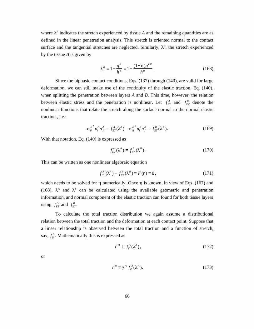
66

where A indicates the stretch experienced by tissue A and the remaining quantities are as

defined in the linear penetration analysis. This stretch is oriented normal to the contact

surface and the tangential stretches are neglected. Similarly, B, the stretch experienced

by the tissue B is given by

B = 1−gB

hB =1−(1− )gTot

hB . (168)

Since the biphasic contact conditions, Eqs. (137) through (140), are valid for large

deformation, we can still make use of the continuity of the elastic traction, Eq. (140),

when splitting the penetration between layers A and B. This time, however, the relation

between elastic stress and the penetration is nonlinear. Let fETA and fET

B denote the

nonlinear functions that relate the stretch along the surface normal to the normal elastic

traction., i.e.:

ijE A

niAn j

A = fETA ( A ) ij

E B

niBn j

B = fETB ( B ). (169)

With that notation, Eq. (140) is expressed as

fETA ( A ) = fET

B ( B ). (170)

This can be written as one nonlinear algebraic equation

fETA ( A ) − fET

B ( B ) = F ( ) = 0 , (171)

which needs to be solved for numerically. Once is known, in view of Eqs. (167) and

(168), A and B can be calculated using the available geometric and penetration

information, and normal component of the elastic traction can found for both tissue layers

using fETA and fET

B .

To calculate the total traction distribution we again assume a distributional

relation between the total traction and the deformation at each contact point. Suppose that

a linear relationship is observed between the total traction and a function of stretch,

say, fDA . Mathematically this is expressed as

tTot ∝ fDA ( A ) , (172)

or

tTot = A fDA( A ). (173)

67

where A is the proportionality constant. In a hyperelastic material, a change in the total

traction should cause a disproportional change in stretch, hence fDA is in general a

nonlinear function.

A vectorial equation analogous to Eq. (160) can be written as

t Tot = A fDA ( A )n , (174)

recalling that the total traction is assumed to be parallel to the surface normal n.

Equation (174) is integrated to obtain a relationship with the total force F.

tiTot dΓc

Γ c

∫ = A fDA ( A )

Γ c

∫ ni dΓc = Fi. (175)

As in the linear penetration analysis, using the magnitude of the resultant force known

from experiment and Eq. (175), A is found to be

A =F

fDA ( A )n idΓc

Γ c

∫

2

i=1

3

∑. (176)

Finally, from Eq. (148) the following expression for * can be derived using Eqs. (170)

and (173).

* = s + f fETA ( A )

A fDA ( A )

. (177)

The function fETA is determined uniquely from the hyperelastic law. On the other hand,

fDA can be chosen in different ways based on observation, such that it expresses the

relation between the total load and the deformation as precisely as possible.

As an example we can apply the above derivation to the hyperelastic material

described by the Eq. (41). For this material, the relation between stretch and the elastic

stress in a uniaxial deformation is given by (dropping the superscript A, for convenience)

nnE =

12

H M

2 −12 +1 e ( 2 −1), (178)

where HM = 4α0(α1+α2) and β = α1+2α2. HM denotes the initial modulus of the material

(i.e. at zero deformation). For demonstrational purposes, we define fD as

fD( ) =2 −1

2 2 +1 e ( 2 −1). (179)

68

This expression, in view of Eq. (178), is a quantification of the deformation. As pointed

out before other choices based on numerical, analytical or experimental experience are

possible.

Substituting Eqs. (178) and (179) into (177) gives the following simplification

for *

* = s + f H MA

. (180)

Other choices for fD might render the term in the bracket deformation dependent. In any

case, f and s in Eq. (180) refer to current values under finite deformation and are

functions of deformation, hence *, unlike in linear penetration analysis, is deformation-

dependent. f and s can be approximated, again considering a unidirectional deformation

and using Eq. (21), as

s ≈ 0s

, (181)

f ≈1− 0s

= 0f + 0

s (1−1

) , (182)

where the subscript ‘0’ indicates the undeformed values of the phase fractions. With that

approximation * becomes

* = 0s

+ 0f + 0

s(1−1

)

H MA

. (183)

For consistency, Eq. (183) should reduce to Eq. (166) as the deformation becomes

infinitesimal. This can be easily shown to be the case.

5.5.1 Application and Computer Implementation

As previously noted, the penetration analysis described above is applied

separately as a preprocessing step to both tissues in contact. In other words, the

calculations above are repeated to obtain the contact boundary conditions for tissue B. To

be consistent, the method should return a set of boundary conditions that satisfy

Eqs. (139) and (140).

In the v-p formulation of the biphasic tissue problem, the pressure and total

traction boundary conditions are applied to enforce this load partitioning. Unlike true

contact analysis, which requires nonlinear interaction between the two layers to resolve

69

the unknown area of contact, the inter-layer dependency of this penetration-based contact

analysis occurs in the preprocessing stage. As a result, after preprocessing, the layers can

be analyzed independent of each other.

The finite element formulation applies a finite difference scheme for time

interpolation that is described in detail in Chapter 4. For a given motion, a set of contact

boundary conditions are derived for each discrete time point and applied at the

corresponding time step to simulate the relative movement of the contacting layers. The

solid modeler package that is utilized in the penetration calculations is Parasolid which is

interfaced to Trellis, the SCOREC finite element framework. The procedure described

above is accomplished by using finite element libraries in Trellis, including the interface

to Parasolid, in combination with stand-alone programming. An object-oriented

computer code is designed and implemented to accomplish this preprocessing. Many

Parasolid commands are invoked explicitly in the preprocessing software, while some

are accessed through the Trellis interface in the computer code.

Finite element shape functions and mesh are used to perform certain calculations

required by the penetration method. The penetration field (and thus the approximated

deformation field) is expressed in terms of the finite element shape functions, and the

integrals in Eq. (144) are evaluated numerically. The computer code creates as many files

as there are time steps in the analysis. They contain the total traction information

expressed on a grid of support points on the contact surface. In the finite element method,

traction boundary conditions are applied at Gauss points of the mesh faces located in the

contact surface. In general, these points do not coincide with the support points.

Therefore, to determine the traction value at a non-support point, a simple bilinear

interpolation is performed on the parametric coordinate system using the traction values

at the neighboring support points.

70

Chapter 6

Linear Examples

6.1 Introduction

The penetration method is validated in this chapter using a canonical geometry

that is an idealization of a physiological joint contact problem. The kinematic input data

for this penetration example are obtained from a biphasic axisymmetric contact code [25]

and treated as if they originated from visualization data for a joint experiment. Following

validation, the method is demonstrated on physiological shoulder geometries.

6.2 Canonical Examples

The penetration method has been validated for the short-time response of two

canonical problems whose geometry and properties resemble the glenohumeral joint in

the shoulder. The definitions of problem geometry and geometric parameters are shown

in Fig. 16; Table 2 gives the values used in this study. The lower and upper tissue layers

in each case are referred to as A and B respectively. The radii of curvature of the articular

and bone surfaces are referred to as RAc and RAb, respectively, for the lower layer, and RBc

and RBb for the upper layer. The thickness of layers A and B at the axis of rotation are tB

and tA. For case CT the thickness is constant through the layer, and for case VT the

thickness varies with radial position. Layers of rigid, impermeable bone support the

cartilage layers; the lower bone supporting structure is fixed and an axially directed force

is applied to the upper tissue layer through the bone. Note that the bone is not modeled

explicitly, but rather used to transmit boundary conditions and load. The first geometric

model consists of two tissues having the same thickness, but different radii of curvature;

in the second model, tissue A is 50% thicker than tissue B. Note that tissue thickness

varies with position from the axis of rotation. We quantify the congruency of contact as

follows:

1

RBc

−1

RAc

=1

congruency

The first example (CT) is more congruent than the second (VT).

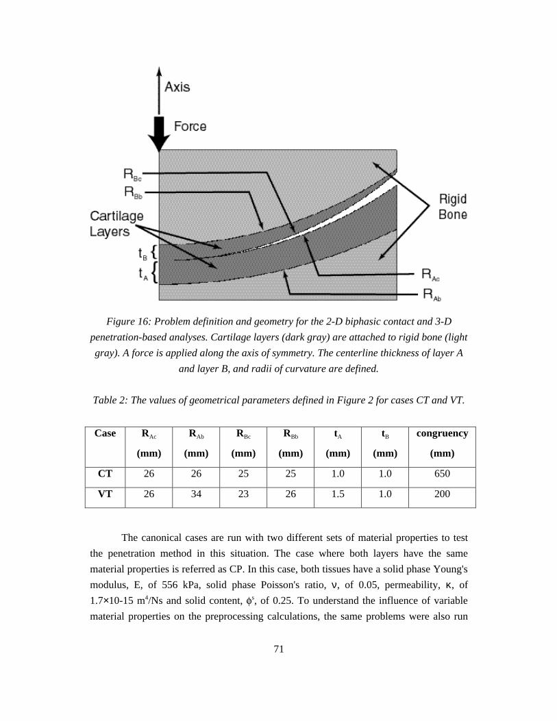
71

Figure 16: Problem definition and geometry for the 2-D biphasic contact and 3-D

penetration-based analyses. Cartilage layers (dark gray) are attached to rigid bone (light

gray). A force is applied along the axis of symmetry. The centerline thickness of layer A

and layer B, and radii of curvature are defined.

Table 2: The values of geometrical parameters defined in Figure 2 for cases CT and VT.

Case RAc

(mm)

RAb

(mm)

RBc

(mm)

RBb

(mm)

tA

(mm)

tB

(mm)

congruency

(mm)

CT 26 26 25 25 1.0 1.0 650

VT 26 34 23 26 1.5 1.0 200

The canonical cases are run with two different sets of material properties to test

the penetration method in this situation. The case where both layers have the same

material properties is referred as CP. In this case, both tissues have a solid phase Young's

modulus, E, of 556 kPa, solid phase Poisson's ratio, ν, of 0.05, permeability, κ, of

1.7×10-15 m4/Ns and solid content, s, of 0.25. To understand the influence of variable

material properties on the preprocessing calculations, the same problems were also run

72

with Young`s modulus halved in layer B. In this second case, referred to as VP, the

material properties of tissue A are the same as in Case CP, but the tissue B has a Young`s

modulus of 278 kPa, half of the value of tissue A. A force of 75 N is applied to the rigid

bone of the upper layer over a linear 1.0 sec. ramp, then held constant for an additional

1.0 sec. Simulations were carried out for the full 2.0 sec. time period.

Each configuration is first analyzed using the 2-D axisymmetric biphasic contact

finite element [26], serving in this validation as the “experimental” data for the

penetration-based method, from which the displacement of the upper rigid body at

t = 2.0s is computed. This computed displacement value is then applied within the solid

modeler to the upper layer of the 3-D solid model, allowing it to rigidly penetrate the

lower layer of the model. Preprocessing starts by quantifying this penetration. After

obtaining the total traction and elastic traction, as described earlier, the corresponding 3-

D analysis is run using a time step of ∆t = 0.1 s. Results obtained at t = 1.0 sec. are

compared with those obtained from the 2-D biphasic contact analysis.

6.2.1 Results for Case CT

Case CT constitutes a highly congruent geometry, and the radii of curvature for

the contacting tissues are close to those of a human shoulder joint. In addition to

validating the penetration method by comparison to a 2-D axisymmetric biphasic contact

analysis, case CT is used to demonstrate the self-consistency of the penetration method,

in terms of the satisfaction of the contact boundary conditions, and the validity of the

assumptions used in deriving the penetration method.

Figures 17 and 18 compare the pressure and normal elastic traction distribution on

the contacting faces of tissues A and B for cases CP and VP, respectively. Note that on

these faces, pressure and normal elastic traction are boundary conditions originating from

the penetration analysis. The pressure and normal elastic traction have similar

distributions on the contacting tissues, indicating that the penetration method produces

boundary conditions that are consistent with the kinetic contact continuity requirements,

Eqs. (139) and (140).

The kinematic contact conditions, Eqs (137) and (138), are not directly enforced

by the penetration method. Rather, the displacement and velocity results in the zone of

contact are computed by the independent 3-D biphasic analyses. It is therefore important

to determine if the deformation of the tissues is consistent with contact.

In the full biphasic contact analysis, layers A and B are in contact only along at

the center (r=0) before the load is applied. Away from this point, there is a gap between

73

the layer geometries that becomes larger with increasing radial distance. In contact, the

displacements of layers A and B should match exactly at the axial contact point. Farther

from that point, the tissue layers first deform without contacting each other, closing the

local gap, and then start to deform together. The axial displacement results in the contact

region of tissues A and B, obtained from the penetration-based 3-D biphasic analysis

appear to support this behavior. The axial displacement results shown in Fig. (19) for

case CP indicate a relatively close match between the axial displacement values close to

the axis. The small deviation between the curves at this point indicates that layer A is

displaced slightly more than layer B leaving a small gap. Considering the approximate

nature of the method, this error is found to be reasonably small. Away from the initial

contact point, the compressive displacement of layer A decreases, reaching positive

displacement values eventually. This corresponds to the ‘bulging’ of the tissue commonly

observed in biphasic materials. Layer B bulges less since it is convex rather than concave.

Still, around r = 5 mm, layer B experiences minimal displacement. That means that the

model gap at this point is closed mostly by the upward bulging of layer A. For case VP,

as shown in Fig. (20), the displacement mismatch tends to become larger if one of the

tissues is significantly more compliant than the other. However, the displacement

behavior of individual layers is the same; bulging is still more prominent on layer A.

In general, it is observed that the velocity, being the derivative of displacement,

tends to fluctuate more then the displacement. Figure (21) shows the normal velocity

distribution of layers A and B for case CP originating from a more refined penetration

analysis where the change in the contact area during ramp phase has been taken into

account. While this pushes the velocity values towards more meaningful numbers, the

mismatch between the results for layers A and B seems to be still high for this quantity.

The error close to the edge of the contact is generally large because, unlike contact

analysis, there is no ‘opposing tissue’ in the penetration analysis that constrains the

velocity. Similar to what is observed for displacement, the error for velocity is larger for

case VP (Fig. (22)).

Figures (23) and (24) compare the magnitude of the elastic traction on layers A

and B for cases CP and VP, respectively, with the corresponding shear stress components

in the planes parallel to the axis. In frictionless contact, all shear stress components

should vanish at the contact interface. The penetration-based analysis gives shear stress

values that are much smaller than the elastic traction, indicating that the applied loading

is a close approximation to frictionless contact.

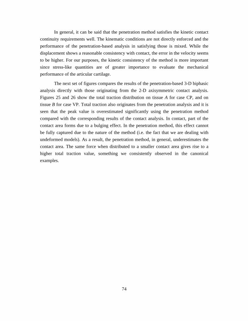
74

In general, it can be said that the penetration method satisfies the kinetic contact

continuity requirements well. The kinematic conditions are not directly enforced and the

performance of the penetration-based analysis in satisfying those is mixed. While the

displacement shows a reasonable consistency with contact, the error in the velocity seems

to be higher. For our purposes, the kinetic consistency of the method is more important

since stress-like quantities are of greater importance to evaluate the mechanical

performance of the articular cartilage.

The next set of figures compares the results of the penetration-based 3-D biphasic

analysis directly with those originating from the 2-D axisymmetric contact analysis.

Figures 25 and 26 show the total traction distribution on tissue A for case CP, and on

tissue B for case VP. Total traction also originates from the penetration analysis and it is

seen that the peak value is overestimated significantly using the penetration method

compared with the corresponding results of the contact analysis. In contact, part of the

contact area forms due to a bulging effect. In the penetration method, this effect cannot

be fully captured due to the nature of the method (i.e. the fact that we are dealing with

undeformed models). As a result, the penetration method, in general, underestimates the

contact area. The same force when distributed to a smaller contact area gives rise to a

higher total traction value, something we consistently observed in the canonical

examples.

75

-100

0

100

200

300

400

500

600

0 5 10 15

A - norm. elas. tract.

A - pressure

B - norm. elas. tract.

B - pressurep

ress

ure

- n

orm

al e

last

ic t

ract

ion

(kP

a)

radial distance (mm)

Figure 17: Case CT-CP, comparison of pressure and normal elastic traction distribution

on layers A and B, t = 1 sec.

-100

0

100

200

300

400

500

600

0 5 10 15

A - pressure

A - norm. elas. tract.B - pressure


pre

ssu

re -

no

rmal

ela

stic

tra

ctio

n (

kPa)


Figure 18: Case CT-VP, comparison of pressure and normal elastic traction distribution


76

-0.06

-0.04

-0.02

0

0.02

0.04

0.06

0 2 4 6 8

A - axial displacementB - axial displacement

axia

l d

isp

lace

men

t (m

m)


Figure 19: Case CT-CP, the axial displacement at the contact interface of layers A and

B, t = 1 sec.

-0.04

-0.02

0

0.02

0.04

0.06

0 2 4 6 8

B - axial displacementA - axial displacement

axia

l d

isp

lace

men

t (m

m)


Figure 20: Case CT-VP, the axial displacement at the contact interface of layers A and

B, t = 1 sec.

77

-0.04

-0.03

-0.02

-0.01

0

0.01

0.02

0 2 4 6 8

A - normal velocityB - normal velocity

no

rmal

vel

oci

ty (

mm

/s)


Figure 21: Case CT-CP, the normal velocity at the contact interface of layers A and B,

t = 1 sec.

-0.04

-0.03

-0.02

-0.01

0

0.01

0.02

0.03

0.04

0 2 4 6 8

B - normal velocityA - normal velocity

no

rmal

vel

oci

ty (

mm

/s)


Figure 22: Case CT-VP, the normal velocity at the contact interface of layers A and B,

t = 1 sec.

78

-25

-20

-15

-10

-5

0

5

10

0 5 10 15

normal elasic tractionshear stress in t

1-n plane

shear stress in t2-n planen

orm

al

ela

sti

c t

rac

tio

n -

sh

ea

r s

tre

ss

(k

Pa

)


Figure 23: Case CT-CP, tissue A, comparison of the normal elastic traction with the

shear stress components in the planes along the normal direction, t = 1 sec.

-20

-15

-10

-5

0

5

10

0 5 10 15

normal elastic tractionshear stress in t

1-n plane

shear stress in t2-n planen

orm

al

ela

sti

c t

rac

tio

n -

sh

ea

r s

tre

ss

(k

Pa

)


Figure 24: Case CT-VP, tissue B, comparison of the normal elastic traction with the

shear stress components in the planes along the normal direction, t = 1 sec.

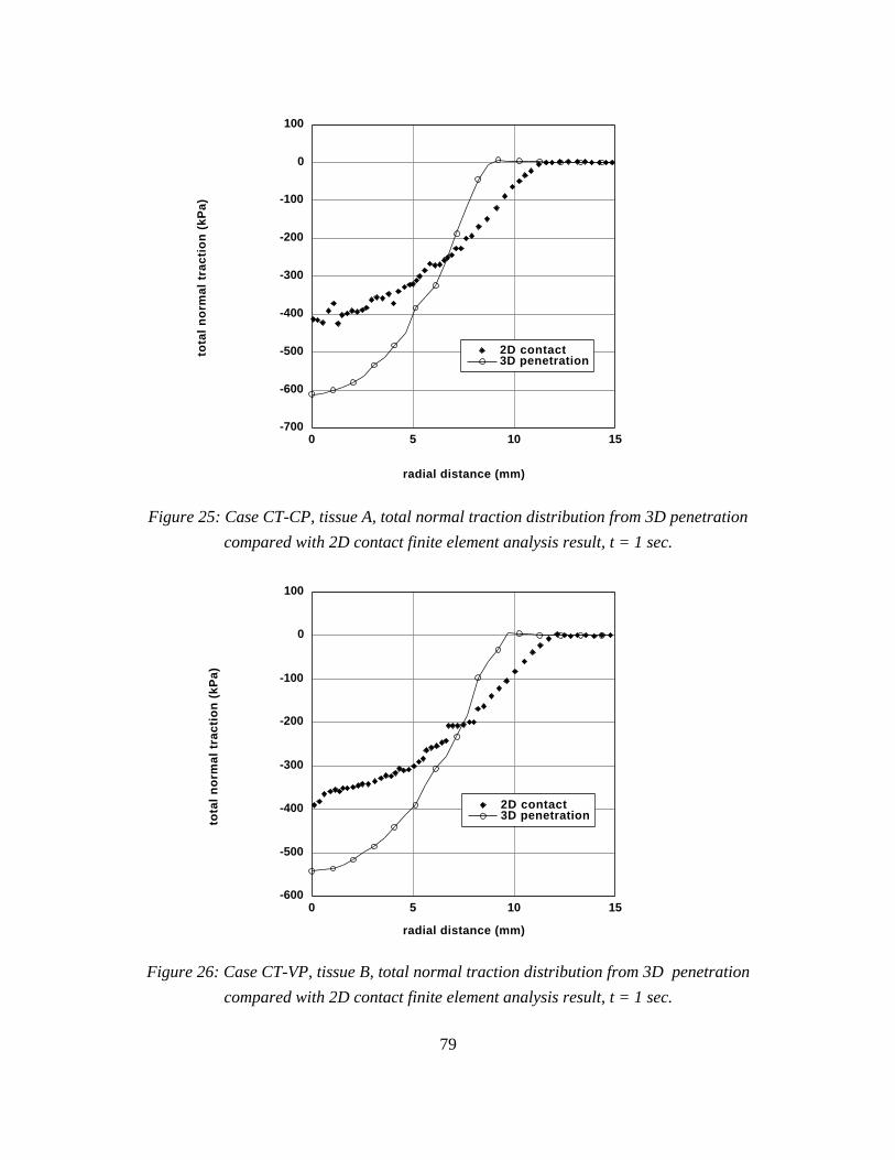
79

-700

-600

-500

-400

-300

-200

-100

0

100

0 5 10 15

2D contact3D penetration

tota

l n

orm

al t

ract

ion

(kP

a)


Figure 25: Case CT-CP, tissue A, total normal traction distribution from 3D penetration

compared with 2D contact finite element analysis result, t = 1 sec.

-600

-500

-400

-300

-200

-100

0

100

0 5 10 15

2D contact3D penetrationto

tal

no

rmal

tra

ctio

n (

kPa)


Figure 26: Case CT-VP, tissue B, total normal traction distribution from 3D penetration


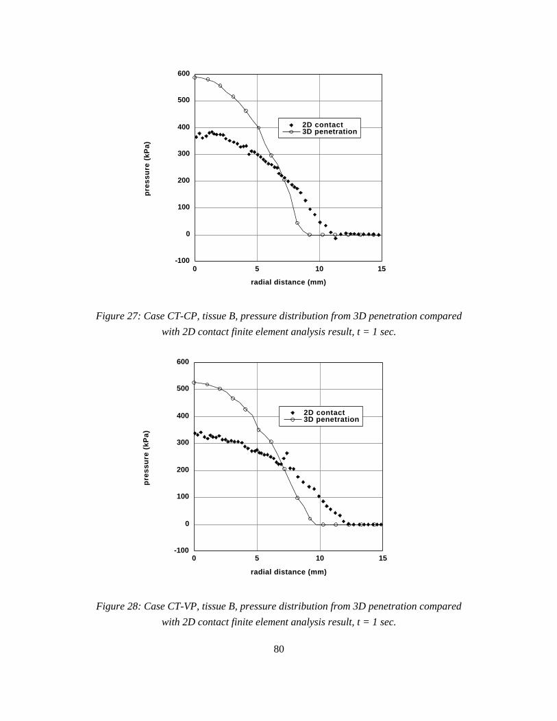
80

-100

0

100

200

300

400

500

600

0 5 10 15


pre

ss

ure

(k

Pa

)


Figure 27: Case CT-CP, tissue B, pressure distribution from 3D penetration compared

with 2D contact finite element analysis result, t = 1 sec.

-100

0

100

200

300

400

500

600

0 5 10 15


pre

ss

ure

(k

Pa

)


Figure 28: Case CT-VP, tissue B, pressure distribution from 3D penetration compared


81

A similar trend is observed in the contact pressure values. Figures 27 and 28

display typical pressure results where it is clear that the penetration method overestimates

the pressure on the contact interface.

Normal elastic traction distribution, particularly the peak values, on layers A and

B for cases CP and VP compare well with values obtained from axisymmetric contact

analysis, as depicted on Figures 29 through 32. Note that the elastic traction, in general, is

much smaller compared to the total traction in magnitude; hence the contact analysis

result for this quantity looks scattered. Recall that in the penetration analysis, the normal

elastic stress is assumed to be relatively uniform through the thickness and calculated

accordingly from penetration, tissue thickness and the modulus (See Eq.(156)). The

results confirm that this assumption is reasonably close to reality for this particular

geometry. The effect of the underestimated contact radius is again visible as we approach

the edge of the contact region.

Figures 33-36 show the axial displacement results on tissues A and B for cases CP

and VP. In this figure, the displacement values are expressed relative to the rigid bone

underlying layer A in each case to facilitate comparison with the contact analysis. In the

finite element analysis, axial displacement is a calculated quantity and not a prescribed

one. Recall that, the axial translation of the rigid bone underlying layer B obtained from

the contact analysis provided the input data to derive the tractions in the penetration

preprocessing. As seen the penetration-based finite element analysis returns displacement

values close to those that are initially used in the penetration method, implying the

consistency of the penetration approach as a whole. Another feature that is captured

qualitatively is the positive displacements at the edge of contact.

Normal velocity on layers A and B for case CP, as shown in Fig. 37, deviate from

each other in both approaches which is consistent with what is observed in Figs. 21-22.

The sudden change close to the edge of contact is qualitatively captured by the

penetration method. For case VP, the contact analysis results start to become scattered

hence a comparison for that case is not shown here. Case VP appears to constitute a more

difficult numerical problem for the contact analysis.

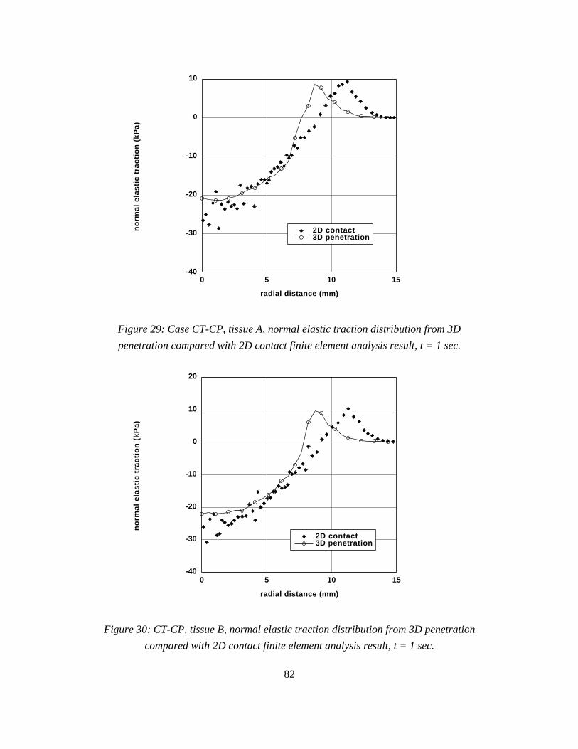
82

-40

-30

-20

-10

0

10

0 5 10 15


no

rmal

ela

stic

tra

ctio

n (

kPa)


Figure 29: Case CT-CP, tissue A, normal elastic traction distribution from 3D

penetration compared with 2D contact finite element analysis result, t = 1 sec.

-40

-30

-20

-10

0

10

20

0 5 10 15


no

rmal

ela

stic

tra

ctio

n (

kPa)


Figure 30: CT-CP, tissue B, normal elastic traction distribution from 3D penetration


83

-25

-20

-15

-10

-5

0

5

10

0 5 10 15


no

rma

l e

las

tic

tra

cti

on

(k

Pa

)


Figure 31: Case CT-VP, tissue A, normal elastic traction distribution from 3D


-25

-20

-15

-10

-5

0

5

10

0 5 10 15


no

rma

l e

las

tic

tra

cti

on

(k

Pa

)


Figure 32: Case CT-VP, tissue B, normal elastic traction distribution from 3D


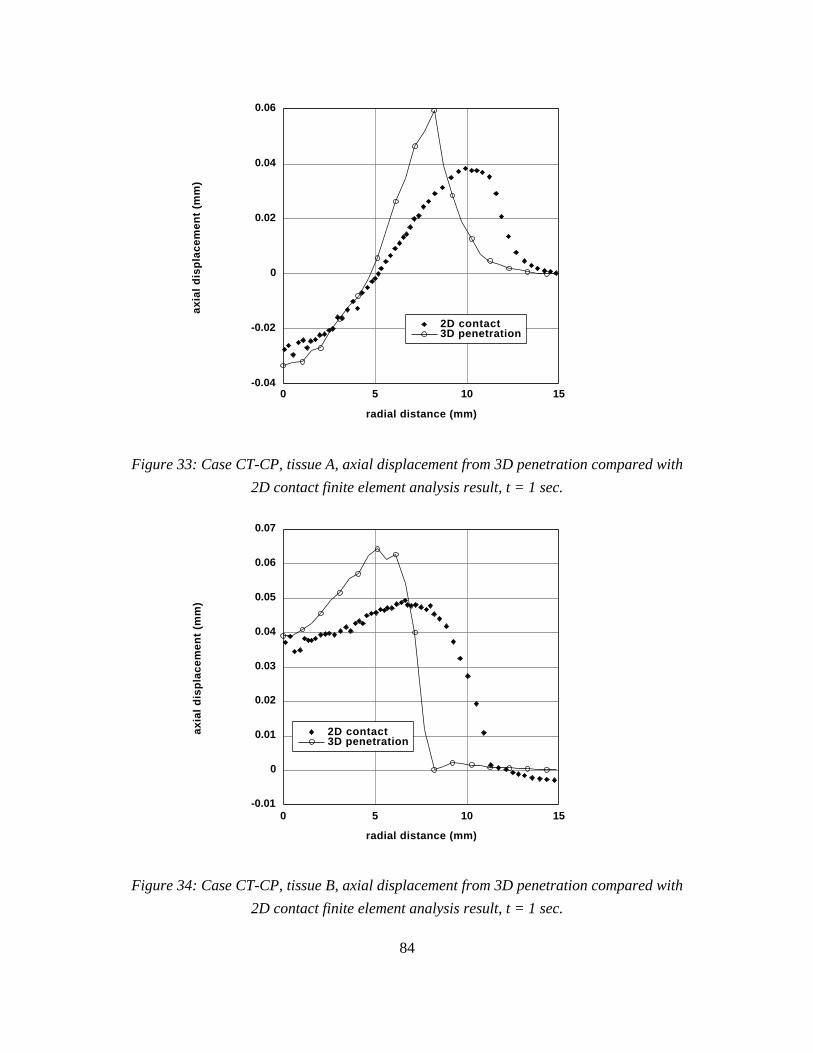
84

-0.04

-0.02

0

0.02

0.04

0.06

0 5 10 15


axia

l d

isp

lace

men

t (m

m)


Figure 33: Case CT-CP, tissue A, axial displacement from 3D penetration compared with

2D contact finite element analysis result, t = 1 sec.

-0.01

0

0.01

0.02

0.03

0.04

0.05

0.06

0.07

0 5 10 15


axia

l d

isp

lace

men

t (m

m)


Figure 34: Case CT-CP, tissue B, axial displacement from 3D penetration compared with


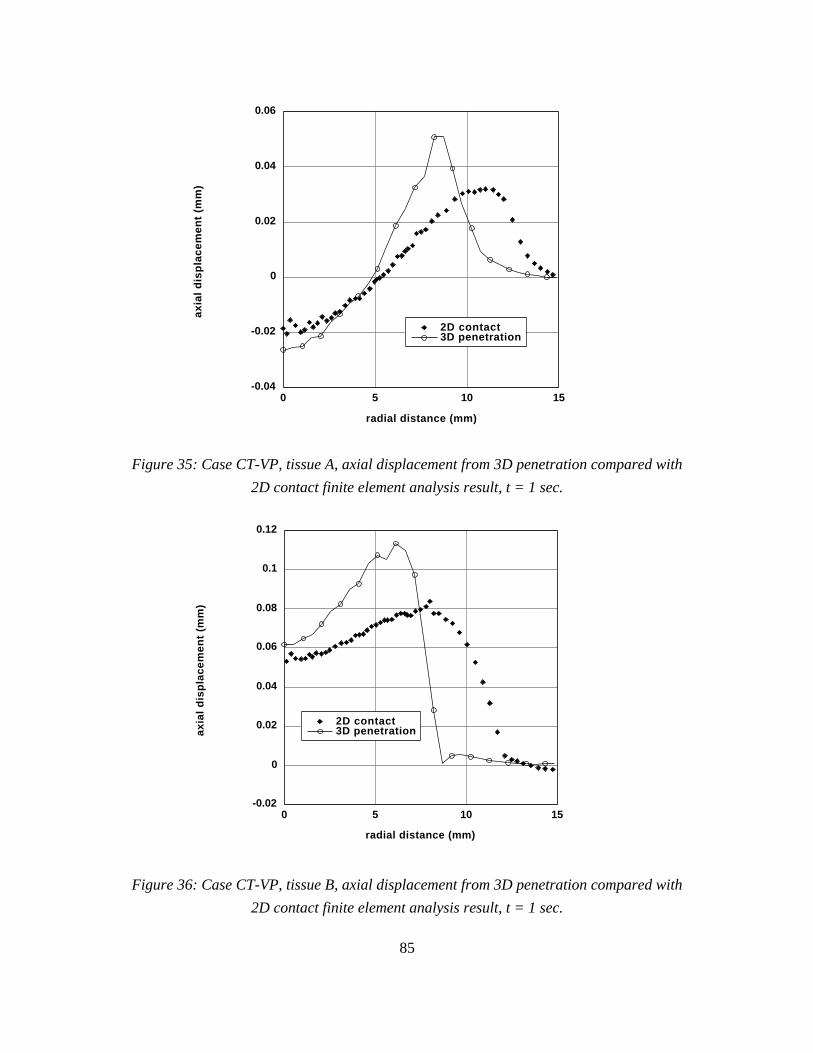
85

-0.04

-0.02

0

0.02

0.04

0.06

0 5 10 15


axia

l d

isp

lace

men

t (m

m)


Figure 35: Case CT-VP, tissue A, axial displacement from 3D penetration compared with


-0.02

0

0.02

0.04

0.06

0.08

0.1

0.12

0 5 10 15

2D contact3D penetrationax

ial

dis

pla

cem

ent

(mm

)


Figure 36: Case CT-VP, tissue B, axial displacement from 3D penetration compared with


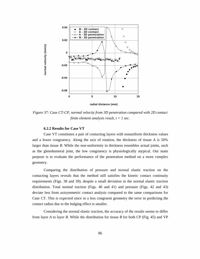
86

-0.06

-0.04

-0.02

0

0.02

0.04

0 5 10 15

B - 2D contactA - 2D contactA - 3D penetrationB - 3D penetration

no

rmal

vel

oci

ty (

mm

/s)


Figure 37: Case CT-CP, normal velocity from 3D penetration compared with 2D contact

finite element analysis result, t = 1 sec.

6.2.2 Results for Case VT

Case VT constitutes a pair of contacting layers with nonuniform thickness values

and a lower congruency. Along the axis of rotation, the thickness of tissue A is 50%

larger than tissue B. While the non-uniformity in thickness resembles actual joints, such

as the glenohumeral joint, the low congruency is physiologically atypical. Our main

purpose is to evaluate the performance of the penetration method on a more complex

geometry.

Comparing the distribution of pressure and normal elastic traction on the

contacting layers reveals that the method still satisfies the kinetic contact continuity

requirements (Figs. 38 and 39), despite a small deviation in the normal elastic traction

distribution. Total normal traction (Figs. 40 and 41) and pressure (Figs. 42 and 43)

deviate less from axisymmetric contact analysis compared to the same comparisons for

Case CT. This is expected since in a less congruent geometry the error in predicting the

contact radius due to the bulging effect is smaller.

Considering the normal elastic traction, the accuracy of the results seems to differ

from layer A to layer B. While the distribution for tissue B for both CP (Fig. 45) and VP

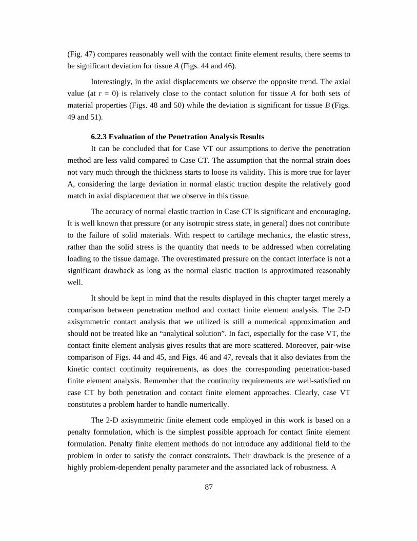
87

(Fig. 47) compares reasonably well with the contact finite element results, there seems to

be significant deviation for tissue A (Figs. 44 and 46).

Interestingly, in the axial displacements we observe the opposite trend. The axial

value (at r = 0) is relatively close to the contact solution for tissue A for both sets of

material properties (Figs. 48 and 50) while the deviation is significant for tissue B (Figs.

49 and 51).

6.2.3 Evaluation of the Penetration Analysis Results

It can be concluded that for Case VT our assumptions to derive the penetration

method are less valid compared to Case CT. The assumption that the normal strain does

not vary much through the thickness starts to loose its validity. This is more true for layer

A, considering the large deviation in normal elastic traction despite the relatively good

match in axial displacement that we observe in this tissue.

The accuracy of normal elastic traction in Case CT is significant and encouraging.

It is well known that pressure (or any isotropic stress state, in general) does not contribute

to the failure of solid materials. With respect to cartilage mechanics, the elastic stress,

rather than the solid stress is the quantity that needs to be addressed when correlating

loading to the tissue damage. The overestimated pressure on the contact interface is not a

significant drawback as long as the normal elastic traction is approximated reasonably

well.

It should be kept in mind that the results displayed in this chapter target merely a

comparison between penetration method and contact finite element analysis. The 2-D

axisymmetric contact analysis that we utilized is still a numerical approximation and

should not be treated like an “analytical solution”. In fact, especially for the case VT, the

contact finite element analysis gives results that are more scattered. Moreover, pair-wise

comparison of Figs. 44 and 45, and Figs. 46 and 47, reveals that it also deviates from the

kinetic contact continuity requirements, as does the corresponding penetration-based

finite element analysis. Remember that the continuity requirements are well-satisfied on

case CT by both penetration and contact finite element approaches. Clearly, case VT

constitutes a problem harder to handle numerically.

The 2-D axisymmetric finite element code employed in this work is based on a

penalty formulation, which is the simplest possible approach for contact finite element

formulation. Penalty finite element methods do not introduce any additional field to the

problem in order to satisfy the contact constraints. Their drawback is the presence of a

highly problem-dependent penalty parameter and the associated lack of robustness. A

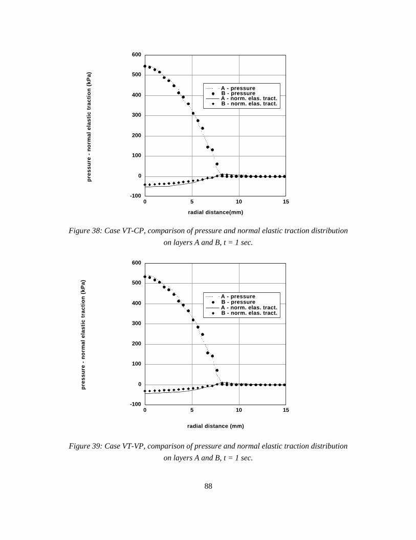
88

-100

0

100

200

300

400

500

600

0 5 10 15

A - pressure

A - norm. elas. tract.B - pressure


pre

ssu

re -

no

rmal

ela

stic

tra

ctio

n (

kPa)

radial distance(mm)

Figure 38: Case VT-CP, comparison of pressure and normal elastic traction distribution


-100

0

100

200

300

400

500

600

0 5 10 15

B - pressure


A - pressure

A - norm. elas. tract.

pre

ssu

re -

no

rmal

ela

stic

tra

ctio

n (

kPa)


Figure 39: Case VT-VP, comparison of pressure and normal elastic traction distribution


89

-700

-600

-500

-400

-300

-200

-100

0

100

0 5 10 15


tal

no

rmal

tra

ctio

n (

kPa)


Figure 40: Case VT-CP, tissue A, total normal traction distribution from 3D penetration


-600

-500

-400

-300

-200

-100

0

100

0 5 10 15


tal

no

rmal

tra

ctio

n (

kPa)


Figure 41: Case VT-VP, tissue B, total normal traction distribution from 3D penetration


90

-100

0

100

200

300

400

500

600

0 5 10 15


pre

ssu

re (

kPa)


Figure 42: Case VT-CP, tissue B, pressure distribution from 3D penetration compared


-100

0

100

200

300

400

500

600

0 5 10 15


pre

ss

ure

(k

Pa

)


Figure 43: Case VT-VP, tissue A, pressure distribution from 3D penetration compared


91

-120

-100

-80

-60

-40

-20

0

20

40

0 5 10 15

2D contact3D penetrationn

orm

al e

last

ic t

ract

ion

(kP

a)


Figure 44: Case VT-CP, tissue A, normal elastic traction distribution from 3D


-80

-60

-40

-20

0

20

0 5 10 15


no

rmal

ela

stic

tra

ctio

n (

kPa)


Figure 45: Case VT-CP, tissue B, normal elastic traction distribution from 3D


92

-100

-80

-60

-40

-20

0

20

0 5 10 15


no

rmal

ela

stic

tra

ctio

n (

kPa)


Figure 46: Case VT-VP, tissue A, normal elastic traction distribution from 3D


-60

-40

-20

0

20

40

0 5 10 15


no

rmal

ela

stic

tra

ctio

n (

kPa)


Figure 47: Case VT-VP, tissue B, normal elastic traction distribution from 3D


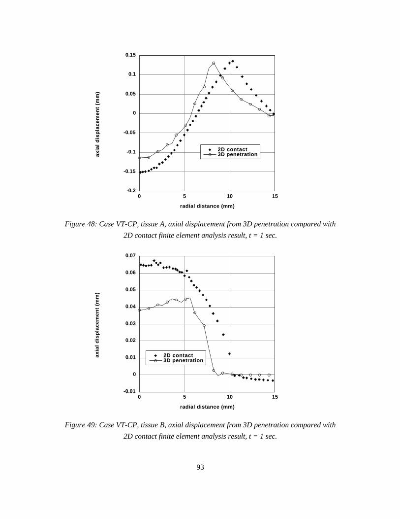
93

-0.2

-0.15

-0.1

-0.05

0

0.05

0.1

0.15

0 5 10 15

2D contact3D penetrationax

ial

dis

pla

cem

ent

(mm

)


Figure 48: Case VT-CP, tissue A, axial displacement from 3D penetration compared with


-0.01

0

0.01

0.02

0.03

0.04

0.05

0.06

0.07

0 5 10 15


axia

l d

isp

lace

men

t (m

m)


Figure 49: Case VT-CP, tissue B, axial displacement from 3D penetration compared with


94

-0.15

-0.1

-0.05

0

0.05

0.1

0.15

0 5 10 15


axia

l d

isp

lace

men

t (m

m)


Figure 50: Case VT-VP, tissue A, axial displacement from 3D penetration compared with


-0.04

-0.02

0

0.02

0.04

0.06

0.08

0.1

0.12

0 5 10 15


axia

l d

isp

lace

men

t (m

m)


Figure 51: Case VT-VP, tissue B, axial displacement from 3D penetration compared with


95

more sophisticated approach would be to use (as often done in finite element analysis)

Lagrange multipliers to satisfy the continuity constraint. The higher accuracy and

improved robustness of this approach comes with a price of higher computational

resources necessary, since additional unknowns are introduced to the problem that need

to be solved for. Hence, a proper 3-D contact finite element analysis can be

computationally overwhelming. From that point of view, penetration method looks like a

reasonable alternative that requires significantly less computational power and provides a

reasonable accuracy and robustness.

6.3 Glenohumeral Analysis

In this section, penetration method is demonstrated on a physiological example,

namely the glenohumeral joint (GHJ) contact of the shoulder. The anatomy of the

shoulder joint with contacting glenoid and humerus cartilages highlighted is shown in

Fig. (52).

The geometry for humeral head and glenoid cartilage have been determined

through SPG from cadaver shoulder joints in the Orthopaedic Research Laboratory at

Columbia University. The tissue kinematics and the total force on the joint obtained for

different elevation angles of the humerus provides the raw data for the penetration

method. The magnitude of the force depends on the elevation angle and varied between

50-185 N in this study. Both tissue layers have material parameters typical for human

joint [40]; namely, Young's modulus, E, of 407 kPa, solid phase Poisson's ratio, , of

0.05, solid content, s of 0.25, permeability, , of 1.2×10-14 m4/Ns. The SPG method

cannot produce deformation information in physiological time ranges such as a second,

and the data obtained for our simulation likely corresponds to deformation that took place

over several minutes in the laboratory (although we are not certain of the exact time).

Still, the corresponding motion will be treated as if occurring in physiological time. The

simulated motion considered for this demonstration corresponds to an arm elevation from

40˚ to 60 ˚ occurring in 15 sec. With a time step of 1 sec., the traction distribution at 40˚

was first applied in a ramp of 5 sec., then the elevation angle was changed by 2˚ at each

time step and the traction distribution and pressure (which are, in general, different both

96

Figure 52: Shoulder geometry with glenoid and humerus cartilages.

in magnitude and position at different elevation angles) corresponding to that angle was a

applied.

While it is numerically possible to apply a larger angle change in the linear

analysis, the time stepping parameters (and elevation angle changes) were picked in order

to facilitate comparison with the equivalent nonlinear example presented in the next

chapter. An angle change of 2˚ per time step, which is sufficiently small for the

convergence of the nonlinear analysis, was used. As mentioned in Chapter 5, SPG cannot

always capture the whole geometry and may therefore produce artificial edges in the

models (note the unnaturally sharp edges occurring in the SPG models shown at the right

hand side picture of Fig. (52)). In addition to handling an “incomplete” geometric model,

it is also difficult to assign a suitable boundary condition to these artificial edges. Our

experience shows that high loads applied close to the edge may give unrealistic results.

Hence, in order to minimize the effects of these model artifacts, the motion was started at

40˚ elevation angle, when the imprint on the humerus is away from its edge. On the other

hand, being the smaller of the tissues, the loading of the edges in the glenoid cannot be

avoided. The tissue that extends from the cartilage like a meniscus and contributes to the

stability and load distribution is called glenoid labrum [18]. Due to its absence in the

geometric model of the joint, the effect of the edge loading is particularly severe when

analyzing the glenoid cartilage. In the analyses that follow, the side face of the glenoid

model is made impermeable to fluid flux to account partially for the missing labrum.

97

6.3.1 Approximate Contact Boundary Conditions

First it is checked if the penetration methods produce contact boundary conditions

in agreement with kinetic contact continuity conditions, Eqs (139) and (141). Figure (53)

shows the distribution of the magnitude of the total traction and the pressure on the

contacting tissue layers as given by the penetration method at an arm elevation angle of

40˚ degrees. The distribution patterns of both quantities match perfectly on the contacting

tissue layers. The magnitude of the quantities are slightly higher on the glenoid.

When a comparison is done at 60˚ elevation angle a similar trend is observed

(Fig. (54)), although the difference in the magnitude of these boundary condition type of

quantities are smaller compared to a 40˚ elevation.

Numerical experience shows that the number of the grid points at which

penetration is calculated, the fineness of the mesh over which the numerical integration of

penetration (Eq. (1)) is performed can cause a deviation in the magnitude and distribution

of total traction and pressure. With the finer grid and finer mesh, the difference in the

distribution pattern can be completely eliminated; however, some deviation in the

magnitude is unavoidable since the integral is evaluated over slightly different contact

areas. Recall that the penetration procedure is performed on the original undeformed

models. The difference in the curvature of the contacting faces of these models will give

different contact areas (See Fig. 15), which will affect the outcome of the penetration

integration. For this particular model pair, the glenoid peak traction was in general about

10% higher than the humeral head, which is reasonable. For congruent geometries such

as diarthrodial joints a high deviation is not likely to appear.

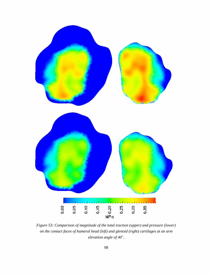
98

Figure 53: Comparison of magnitude of the total traction (upper) and pressure (lower)

on the contact faces of humeral head (left) and glenoid (right) cartilages at an arm

elevation angle of 40˚.

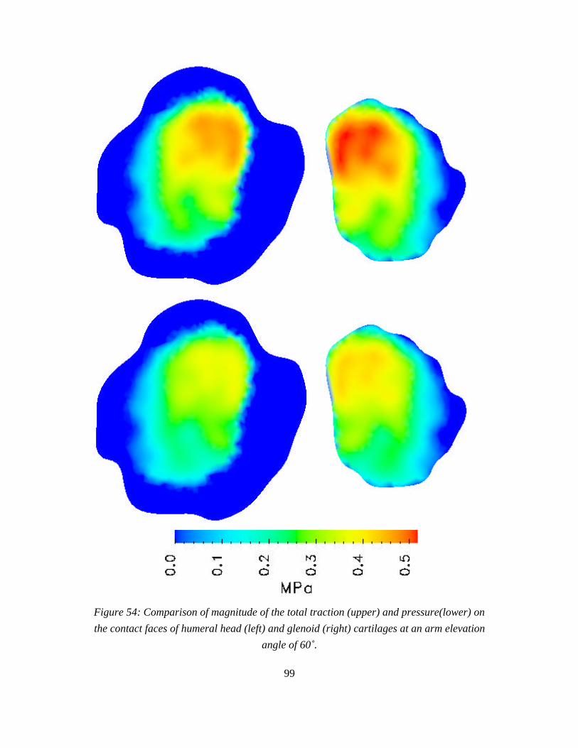
99


the contact faces of humeral head (left) and glenoid (right) cartilages at an arm elevation

angle of 60˚.

100

6.3.2 Humerus Results

For the humeral analysis, a mesh that has six layers of elements through the

thickness of the tissue is used. Numerical observation shows that further through-

thickness refinement does not affect the solution significantly. In total, the mesh is made

of 14819 tetrahedral elements and 30450 nodes. Stress-like quantities are of major

interest since they are related to the tissue performance. They are displayed at three

different times, t = 5,10, and 15 sec. during the motion, corresponding to elevation angles

of 40˚, 50˚ and 60˚ degrees respectively.

Figure 55 shows both a change in the distribution pattern and the magnitude of the

maximum tensile stress on the contacting face. The imprint of the glenoid edges is clearly

visible as high stress areas. It is noted that the stress pattern moves from the inferior

(lower) towards the superior (upper) side of the humerus and the stress increases as the

elevation angle changes. In this range, the force acting on the joint typically increases as

the elevation angle grows; so, part of the increase in the stress with increasing angle can

be attributed to this phenomenon.

An advantage of numerical simulation is that it enables researchers to gain insight

about quantities that are difficult, if not impossible, to measure experimentally such as

stresses at the cartilage bone interface. Figures 56-59 display stress results at the bone

interface of the humerus.

The incongruent loading pattern, typical for diarthrodial joints, is clearly visible in

maximum tensile stress distribution at the bone interface, as depicted in Fig. 56. While

there is a circular high stress region, the center seems to experience relatively low tensile

stresses. The increase in the stress at higher arm elevation is again visible. Note also that

the tensile stresses at bone interface is significantly larger compared to the contacting

face of the tissue. Considering the distribution at 60˚ we observe a highly localized high

stress point.

The maximum compressive stress (Fig. 57) and the maximum shear stress

(Fig. 58) at the bone interface follow a trend similar to maximum tensile stress in terms

of the shape and the evolution of the pattern, and the location of areas of high stress.

Another important observation is that the stress magnitude is close to the maximum

tensile stress for both quantities.

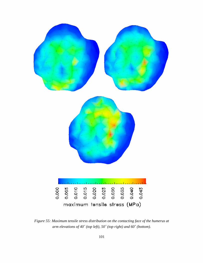
101


arm elevations of 40˚ (top left), 50˚ (top right) and 60˚ (bottom).

102



103


humerus at arm elevations of 40˚ (top left), 50˚ (top right) and 60˚ (bottom).

104

Figure 58: Maximum shear stress distribution on the bone interface of the humerus at


105

6.3.3 The Glenoid Results

The glenoid, in general, experiences stresses that are quantitatively and

qualitatively different than we observe in the humerus. Due to the modeling constrains

mentioned in Section 6.3, it is more difficult to draw firm conclusions on the glenoid

results.

The mesh for the glenoid model has eight layers of elements through the thickness

(note that the glenoid is thicker than the humerus). The number of elements and nodes are

11781 and 24116, respectively.

Considering the physiology of the shoulder joint, the glenoid, being the smaller of

the contacting tissue layers, should not experience drastic pattern changes; this is

confirmed by the maximum tensile stress distribution on the contacting face of the

glenoid, Fig. 59. The stresses are higher at the edges and lower in the center as expected

from the incongruency of this joint. General stress levels increase as the angle increases

(although, due to the scale of the figure, it is not immediately obvious). As the elevation

angle changes, the high stress area seems to shift from the inferior part to the superior

part.

Similar observations can be made when looking at Figs. 60-62. The tensile,

compressive and shear stress pattern on the bone interface follow the same trend as the

maximum tensile stress at the contacting face. While the anterior (front, left hand side in

Fig. 59, right hand side in Figs. (60-62) edge seems to undergo relatively high stresses,

the stress level at the posterior (back) edge is much lower. The magnitudes of maximum

tensile, compressive and shear stresses at the bone interface is not as close to each other

as they are on the humerus. Also, there is not a clear difference in the level of stress that

the contacting face and bone interface experience, unlike what was observed on the

humerus.

6.3.4 Evaluation of the Glenohumeral Analysis Results

Comparison of the total traction and pressure on the contacting faces of the

humerus and glenoid shows that linear penetration method satisfies the kinetic contact

continuity requirements reasonably well.

The results on the humerus confirm what we know about the mechanics of the

diarthrodial joints. For this particular joint model, the average radius of the curvature of

the contacting face of the glenoid is larger than that of the humeral contact face. This

incongruency reflects itself on the stress results as a circular high stress region and a low

stress center.

106


arm elevations of 40˚ (left), 50˚ (center) and 60˚ (right).

Figure 60: Maximum tensile stress distribution on the bone interface of the glenoid at

arm elevations of 40˚ (left), 50˚ (center) and 60˚ (right).

107


at arm elevations of 40˚ (left), 50˚ (center) and 60˚ (right).


elevations of 40˚ (left), 50˚ (center) and 60˚ (right).

108

The short-time asymptotic solution for the contact of linear biphasic tissues gives

equal peak values for the maximum tensile, compressive, and shear stresses in the tissues.

It is encouraging to see that the stress results for the humerus is in agreement with the

trend of the asymptotic solution.

In the glenoid tissue, high stresses seem to concentrate at the edges. While this

makes sense physiologically part of this effect can be attributed to defects of the

geometric glenoid model obtained through SPG. On both faces, the area of peak stress

shifts from inferior to anterior to the superior edge as the elevation angle increases. The

posterior edge does not encounter large stresses, in general.

In the next chapter, it will be seen if and how these observations change in the

case of tissue layers of hyperelastic material with strain dependent permeability.

109

Chapter 7

Nonlinear Examples

7.1 Introduction

In this chapter we will first check the correctness of the developed nonlinear code,

then demonstrate the ability of the nonlinear penetration analysis to satisfy the kinetic

contact continuity conditions on a glenohumeral joint model. It is not possible to test the

nonlinear penetration method the way we tested the linear one in the previous chapter

since a nonlinear biphasic contact code is yet to be developed. A nonlinear penetration-

based finite element analysis will be performed on the same physiological model used in

the linear analysis and the effects of nonlinearity on trends in the results will be observed.

7.2 Confined Compression Examples

Confined compression experiment as depicted by Fig. 1 is a 1-D problem. A plug

of tissue is tightly fit into a chamber and compressed with a highly-permeable, porous

indenter giving rise to a uniaxial motion of the tissue and the interstitial fluid. From an

analytical point of view, confined compression represents an easy problem. However,

numerically, it is a challenging problem due to the existence of steep gradients near the

loaded surface, and has therefore been widely used to test the performance of finite

element codes developed for studies in soft tissue mechanics.

The force-controlled confined compression experiment is called the creep

experiment whereas the displacement controlled one is referred as the stress relaxation

experiment. In this section we compare the results of the nonlinear biphasic finite element

code developed with a converged finite difference solution. While the finite element

analyses are run on a 3-D geometry the finite difference solutions are 1-D. Comparisons

are made for both creep and stress relaxation problems.

7.2.1 Creep

In the confined compression creep (CC-CR) problem, a traction that will result to

an equilibrium stretch of 0.6 is applied as a 5 sec. ramp and held steady. The time step

and integration parameter are t = 0.5 sec. and = 0.6, respectively. The material

properties, typical for soft tissues [40], are selected as α0 = 0.0921 MPa, α1 = 0.9887,

α2 = 0.058158, s0 = 0.2 and 0= 0.00247 mm4/Ns.

110

Figure 63: The finite element mesh used in confined compression problems

The finite element mesh used in the analysis is shown in Fig. 63. The height of the

geometry is 1 mm and there are 64 layers of elements of equal thickness through the

height such that there are a total of 384 elements and 1026 nodes.

Figures 64-66 compare the finite element (indicated as FE in the figure captions)

results for pressure, axial displacement and axial stress with converged finite difference

(indicated as FD in the figure captions) results at various time points. The axial stress

differs slightly from the finite difference solution at t = 10 sec. Otherwise, the agreement

seem to be perfect for all quantities at all times. Numerically, the difference is generally

less than 1 % although the finite difference mesh is much finer than the finite element

mesh.

111

-0.05

0

0.05

0.1

0.15

0.2

0.25

0.3

0.35

0 0.2 0.4 0.6 0.8 1

t = 10 s.t = 50 s.t = 200 s.t = 500 s.

pre

ssu

re (

MP

a)

depth (mm)

Figure 64: Pressure as function of depth at various time point in CC-CR. Solid lines

indicate converged FD results while symbols are FE results.

-0.35

-0.3

-0.25

-0.2

-0.15

-0.1

-0.05

0

0.05

0 0.2 0.4 0.6 0.8 1

t = 10 s.t = 50 s.t = 200 s.t = 500 s.

axia

l d

isp

lace

men

t (m

m)

depth (mm)

Figure 65: Axial displacement as function of depth at various time point in CC-CR. Solid

lines indicate converged FD results while symbols are FE results.

112

-0.35

-0.3

-0.25

-0.2

-0.15

-0.1

-0.05

0

0.05

0 0.2 0.4 0.6 0.8 1

t = 10 s.t = 50 s.t = 200 s.t = 500 s.

axia

l st

ress

(M

Pa)

depth (mm)

Figure 66: Axial stress as function of depth at various time point in CC-CR. Solid lines


7.2.2 Stress Relaxation

In the confined compression stress relaxation (CC-SR) example, a displacement

corresponding to an equilibrium stretch of 0.9 is applied as a ramp of 50 sec. and then

held steady. The time step and integration parameter are t = 1.0 sec. and = 0.6,

respectively. This loading produced stresses close to the maximum value observed in the

creep problem, and thus the nonlinearity was sufficiently strong for the appropriate

testing of the code. The geometry, material properties and the finite element mesh used

are the same as in the creep problem.

Figures 67-69 compare the finite element results for pressure, axial displacement

and axial stress at various time points. In the stress relaxation problem, there is typically a

rapid decay at the point when the ramp reaches its maximum point where numerical

errors are likelier to occur. Figure 67 shows that there is a slight deviation in pressure

from the finite difference solution at deeper zones of the tissue at t = 50 sec. Otherwise,

the agreement with the finite difference solution is perfect for this quantity. (Note the

rapid decay in pressure from t = 50 sec. to t = 60 sec.)

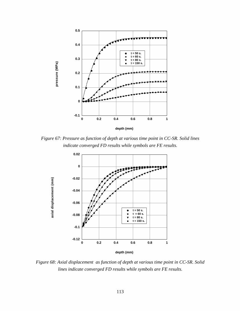
113

-0.1

0

0.1

0.2

0.3

0.4

0.5

0 0.2 0.4 0.6 0.8 1

t = 50 s.t = 60 s.t = 80 s.t = 150 s.

pre

ssu

re (

MP

a)

depth (mm)

Figure 67: Pressure as function of depth at various time point in CC-SR. Solid lines


-0.12

-0.1

-0.08

-0.06

-0.04

-0.02

0

0.02

0 0.2 0.4 0.6 0.8 1

t = 50 s.t = 60 s.t = 80 s.t = 150 s.

axia

l d

isp

lace

men

t (m

m)

depth (mm)

Figure 68: Axial displacement as function of depth at various time point in CC-SR. Solid

lines indicate converged FD results while symbols are FE results.

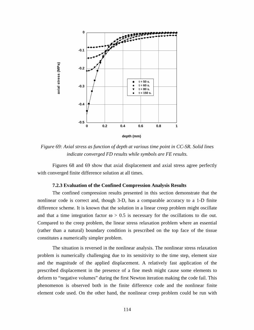
114

-0.5

-0.4

-0.3

-0.2

-0.1

0

0 0.2 0.4 0.6 0.8 1

t = 50 s.t = 60 s.t = 80 s.t = 150 s.ax

ial

stre

ss (

MP

a)

depth (mm)

Figure 69: Axial stress as function of depth at various time point in CC-SR. Solid lines


Figures 68 and 69 show that axial displacement and axial stress agree perfectly

with converged finite difference solution at all times.

7.2.3 Evaluation of the Confined Compression Analysis Results

The confined compression results presented in this section demonstrate that the

nonlinear code is correct and, though 3-D, has a comparable accuracy to a 1-D finite

difference scheme. It is known that the solution in a linear creep problem might oscillate

and that a time integration factor > 0.5 is necessary for the oscillations to die out.

Compared to the creep problem, the linear stress relaxation problem where an essential

(rather than a natural) boundary condition is prescribed on the top face of the tissue

constitutes a numerically simpler problem.

The situation is reversed in the nonlinear analysis. The nonlinear stress relaxation

problem is numerically challenging due to its sensitivity to the time step, element size

and the magnitude of the applied displacement. A relatively fast application of the

prescribed displacement in the presence of a fine mesh might cause some elements to

deform to “negative volumes” during the first Newton iteration making the code fail. This

phenomenon is observed both in the finite difference code and the nonlinear finite

element code used. On the other hand, the nonlinear creep problem could be run with

115

relatively large applied tractions and the Newton iteration converges even on coarser

meshes.

In general, the modified-Newton solver with line search provided stabilization in

both problems against variations in the time step, load level and mesh. Hence,

convergence was achieved for a broad spectrum of problem parameters.

7.3 Glenohumeral Analysis

The glenohumeral analysis of the previous chapter is repeated in this section for

the demonstration of the nonlinear penetration-based finite element method on a

physiological geometry. The experimental data obtained through SPG and utilized in the

previous chapter provides this time the input to the nonlinear penetration procedure as

described in Section 5.3. The resulting total traction and pressure boundary conditions are

applied to the biphasic tissue with a hyperelastic solid phase. The motion simulated is the

same arm elevation motion as in the linear penetration-based analysis described in

Section 6.3.

The hyperelastic material properties of the solid phase are α0 = 0.0921 MPa,

α1 = 0.9887, α2 = 0.058158, with initial permeability, 0 of 0.012 mm4/Ns and initial

solid content, 0s ,of 0.25. Note that at infinitesimal deformation these properties are

equivalent to those used in the linear glenohumeral analysis such that a quantitative

comparison between linear and nonlinear approaches can be made.

7.3.1 Approximate Contact Boundary Conditions

Figures 70 and 71 compare the total traction and pressure boundary conditions at

arm elevations of 40˚ and 60˚, respectively, on the contacting faces of the humerus and

glenoid as calcuted through nonlinear penetration method As in the linear penetration

approach, the resulting boundary conditions have identical distribution patterns and

satisfy the contact kinetic contact continuity requirements reasonably well. The deviation

in peak values between humerus and glenoid is smaller than in the linear penetration

approach.

116



angle of 40˚ originating from nonlinear penetration procedure.

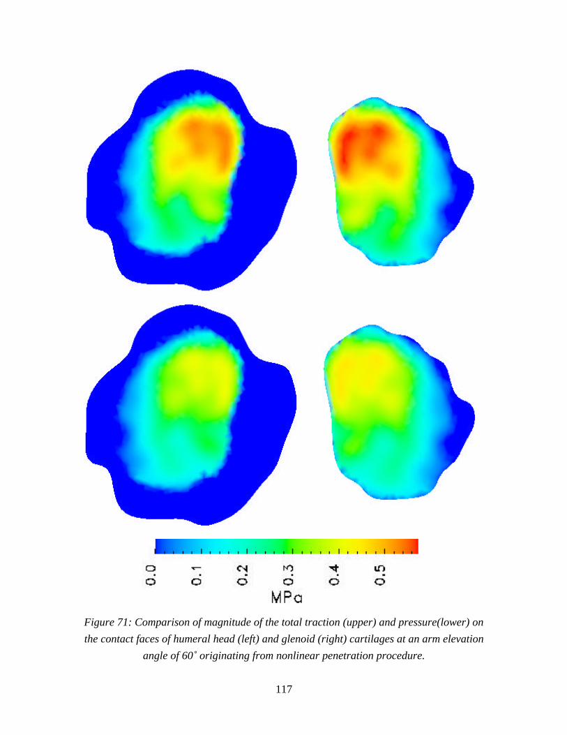
117



angle of 60˚ originating from nonlinear penetration procedure.

118

7.3.2 Humerus Results

To analyze the humerus under finite deformation, the same mesh used in the

linear analysis is utilized here. Various stress quantities are displayed on the contacting

face and the bone interface of the humerus at elevation angles of 40˚, 50˚ and 60˚ in

Figures 72-75.

Figure 72 shows the maximum tensile stress on the contacting face. The

distribution is relatively uniform and the circular loading pattern observed in the linear

analysis is no longer present; however, high stress spots, although smaller, still shifts

from the inferior region to the superior one with increasing elevation angle. The peak

value experienced is more than twice as large compared to the linear analysis (Compare

Fig. 72 with Fig. 55).

The circular loading pattern observed in the linear analysis is also encountered in

the nonlinear analysis when looking at the results for the maximum tensile, compressive

and shear stresses at the bone interface (Figs. 73-75). Their distribution and evolution

with changing arm elevation is almost identical to the linear analysis and the same

qualitative conclusions can be drawn.

Despite the presence of qualitative similarities with the results originating from

the linear analysis, the nonlinear analysis seems to cause major differences quantitatively.

In particular, the nonlinear approach predicts higher tensile stresses (compare Figs. 73

and 56) and lower compressive stresses (compare Figs. 74 and 57) at the bone interface.

The peak values for the maximum shear stress are comparable to the linear analysis.

7.3.3 Glenoid Results

In the previous chapter it was noted that the high stress values occurring at the

edges of the glenoid tissue are partially attributed to model defects originating from the

limitations of the SPG technique and the absence of the glenoid labrum in the mechanical

analysis. Factors that cause poor results in a linear analysis can have more severe effects

in a nonlinear analysis since they can compromise convergence.

It is observed that a nonlinear analysis on the available glenoid geometry could be

run only by constraining the displacement on the side face and making that face

permeable to fluid flow. Still, at higher arm elevations, when the tractions are higher the

code fails to convergence. Thus, the stress results are presented at angles of 40˚ and 50˚,

only.

119


arm elevations of 40˚ (top left), 50˚ (top right) and 60˚ (bottom) degrees.

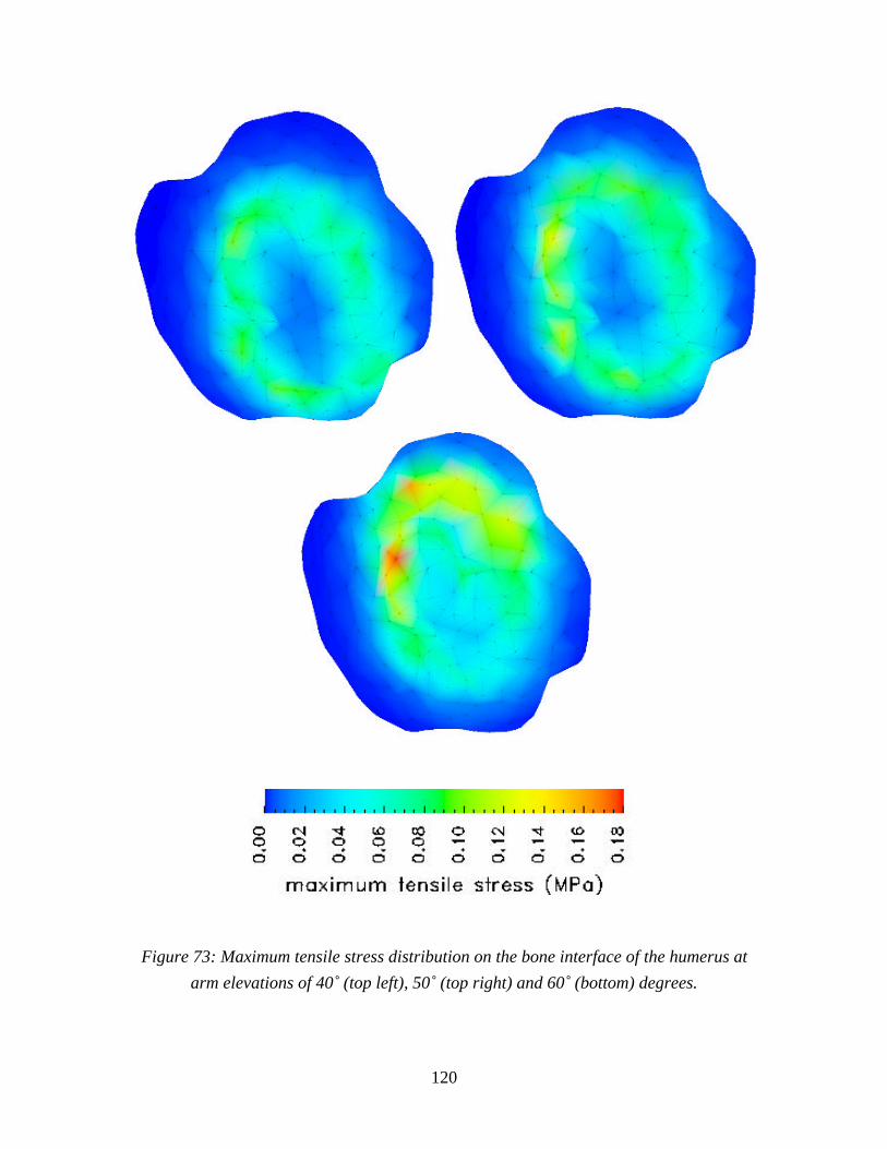
120



121


humerus at arm elevations of 40˚ (top left), 50˚ (top right) and 60˚ (bottom) degrees.

122

Figure 75: Maximum shear stress distribution on the bone interface of the humerus at


123

The maximum tensile stress on the contacting face is displayed in Fig. 76. The

circular stress pattern originating from the nonlinear analysis has disappeared on the

glenoid as it does on the humerus. High stress region move from the inferior to the

superior side with increasing arm elevation. Considering the central part only, the stress

magnitude is larger than in the linear analysis. Closer to the edges, a comparison turns out

to be inconclusive.

Unlike what is observed on the humerus, maximum tensile, compressive and

shear stress at the bone interface of the glenoid does not display the circular incongruency

pattern of the joint (Figs. 77-79). Instead, the stresses are more uniformly distributed.

Due to the vast difference in the picture scales, a visual comparison with the

results of the linear analysis is hard to make; however, a numerical comparison reveals

the following information:

At the central part, maximum tensile stress, in general, is slightly higher than in

the linear analysis. On the other hand, the maximum compressive stress is clearly lower

then the values obtained in the linear analysis, following a similar trend to humerus. The

maximum shear stress values encountered on the glenoid is comparable to those observed

in the linear analysis.

7.3.4 Evaluation of the Glenohumeral Analysis Results

The results presented in the previous three sections indicate that nonlinear finite

element analysis of the contacting biphasic tissue layers can give qualitatively and

quantitatively different results than the linear analysis. The nature of the hyperelastic

solid phase and its the strain-dependent permeability is main factor behind this effect.

Hence, the nonlinearities due to large deformation and strain-dependent permeability of

the solid phase should be accounted for when appropriate for accurate finite element

analysis of the contacting tissues. The derived total traction and pressure boundary

conditions have higher peak values compared to the linear penetration analysis which is

the other factor inducing the difference between linear and nonlinear approaches.

Considering, the relatively large time scale of SPG measurements, the actual

tissues must have been under large deformation when their kinematics were measured.

The boundary conditions derived through nonlinear penetration analysis satisfy the

kinetic contact continuity requirements better than the linear analysis, which seems to

confirm the presence of nonlinear effects in the tissue. Although not explicitly displayed

here, the humerus results also indicate the appropriateness of the uniform through-

thickness pressure assumption made in the penetration derivation.

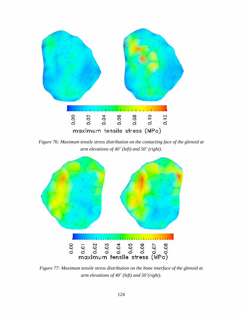
124


arm elevations of 40˚ (left) and 50˚ (right).

Figure 77: Maximum tensile stress distribution on the bone interface of the glenoid at

arm elevations of 40˚ (left) and 50˚(right).

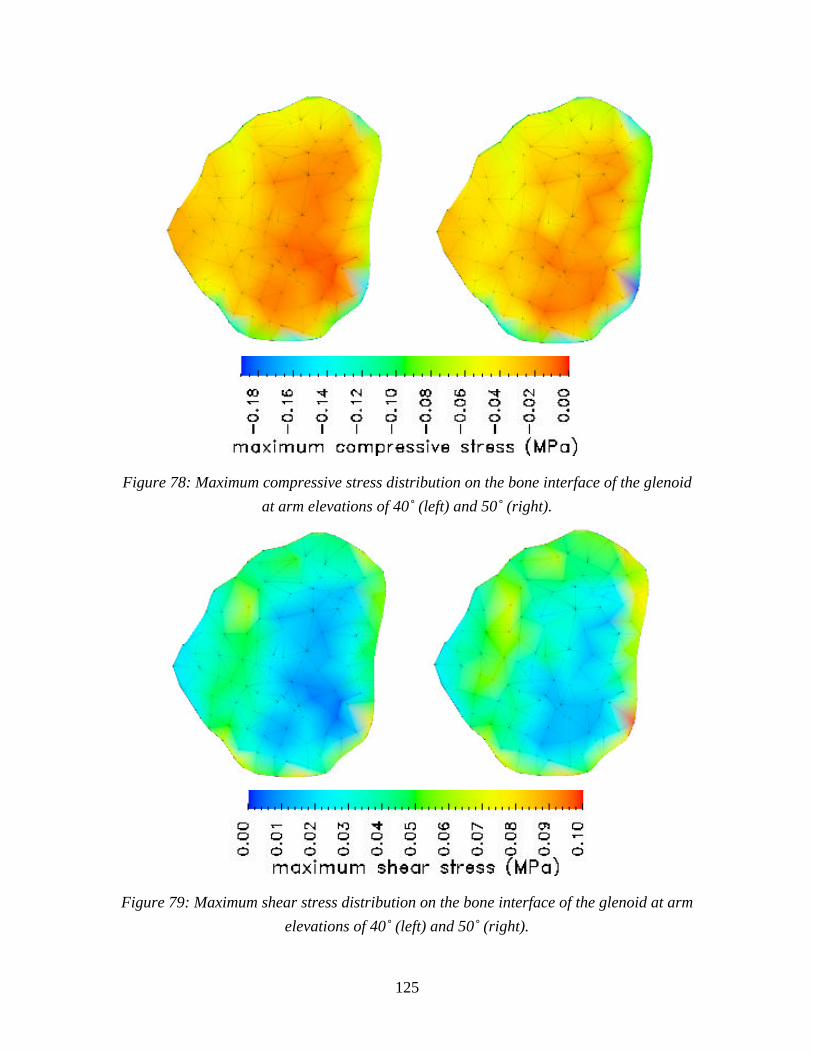
125


at arm elevations of 40˚ (left) and 50˚ (right).


elevations of 40˚ (left) and 50˚ (right).

126

Since there is no independent nonlinear finite element contact program or

analytical solution for nonlinear contact available, the nonlinear penetration procedure

cannot be verified as done for the linear penetration procedure. However, the results

presented in this chapter are thought to be consistent and plausible.

127

Chapter 8

Summary, Conclusions and Future Research

8.1 Summary and Conclusions The ability to predict the response of biphasic soft tissues in contact is

fundamental to the understanding of diarthrodial joint biomechanics, and it represents is a challenging computational mechanic problem. From a mechanics point of view, it requires a representative continuum theory, associated constitutive models, measured materials properties, geometry, kinematic and kinetic conditions, all of which must be validated against experimental and physiological data. The present research represents the initial attempt to analyze soft tissue contact under in vivo conditions, using physiological geometry and loading, taking into account large deformation and strain-dependent permeability of the biphasic tissue layers. An approximate method to simulate the time-dependent deformation of contacting biphasic cartilage layers during in vivo diarthrodial joint motion was developed and implemented. In order to address complex physiological joints, the research addressed three major components:

• Derivation and validation of a penetration-based approximation for 3-D

contact of linear and nonlinear biphasic tissue layers based on the biphasic

governing equations and biphasic contact conditions.

• Evaluation of alternate linearizations of the nonlinear biphasic problem

discretized using a velocity-pressure or displacement-pressure finite element

formulation, together with alternate line search strategies that provide robust

solutions to problems with realistic physiological tissue geometry and material

properties.

• Implementation and testing of these methods within the Trellis analysis

framework in order to allow more systematic analysis of physiological

problems.

The penetration method is a preprocessing technique that uses kinematic data that may originate from various experimental visualization techniques as input. The quantities that must be measured and provided as input for our analysis are: the undeformed geometry and material properties of the contacting tissue layers; the kinematics of the hard tissues to which the tissue layers are attached; and the force vector(s) associated

128

with the motion. In our examples, this data was provided through an experimental study at the Orthopedic Research Laboratory at Columbia University. This data is then imported, and a geometric model of the tissues layers is constructed using commercial modeling software. Assuming the hard tissues are rigid, the kinematic data can be used to position tissue layers physiologically. Since the tissue geometry is the undeformed geometry, the physiological positions will produce tissue overlap, or penetration, whose distribution can be characterized by the solid modeling software.

The penetration method uses the time-dependent penetration distributions, tissue geometry and material properties, and total force vector to calculate approximate contact traction boundary conditions (as a function of time for articulating joints) for each of the contacting tissues. Since this is a preprocessing step, the 3-D linear or nonlinear biphasic analyses can then be performed independently on each of the layers. By this method, the intrinsic nonlinearity of contact is avoided.

The applied tractions in the contact region for each layer were derived based on the linear or nonlinear biphasic governing equations, and the contact boundary conditions for biphasic tissues. Using these equations, and assumptions that are supported by numerical observation or independent studies, the distribution of traction, and the split between the solid and fluid phases (i.e., total traction and pressure), were derived as a function of the penetration distribution, point-wise tissue depth and material properties, and load vector. The derivation was done for both linear and nonlinear hyperelastic biphasic materials, and it applies to any time during the joint articulation. These approximate contact boundary conditions were used in conjunction with linear v-p and, nonlinear v-p and u-p finite element methods to analyze tissue layers in contact.

Several canonical axisymmetric problems (with varying geometry, congruity and material properties), with geometry and properties representative of a human glenohumeral joint, was used to validate the penetration-based linear v-p finite element method. The validation consisted of two steps; first, the 3-D penetration-based biphasic solutions were checked for self-consistency. In this the step the contact boundary conditions and assumptions used in the derivation of the method were examined; second, the 3-D penetration-based solutions were compared with a 2-D axisymmetric biphasic contact analysis to assess the accuracy of the method.

In the self-consistency phase of validation, the results demonstrate approximate satisfaction of the contact boundary conditions. They further demonstrated that the assumptions made in the derivation were appropriate: strain components neglected in the

129

derivation were found to be either small or of no consequence; and the through-thickness distribution of the normal strain and pressure were relatively uniform,

The comparisons with a 2-D axisymmetric contact finite element analysis for the same canonical geometry showed that the penetration-based finite element method produces relatively accurate results for elastic stress and displacement, and that accuracy improved as joint congruity increased. The results for elastic stress were particularly encouraging since this quantity is thought by a number of researches to be particularly relevant to tissue performance.

Based on these results, it is concluded that the penetration method is a reasonable first order approximation to full biphasic contact analysis. The main drawback of the penetration method was that it underestimated the contact area, and as a result, overestimated the total stress and pressure, in general. Also the accuracy of the method dropped close to the edge of the contact area, however, this is not of great concern since stress quantities tend to be lower at that part of the geometry and the maximum values experienced by the tissue are not affected by this error. It is clear that the method is computationally less complex than full contact analysis, and therefore requires less computational resources, however a full study of the method’s accuracy for arbitrary 3-D problems will have to await the development of 3-D biphasic contact methods.

The penetration method has been used to analyze the glenohumeral joint (GHJ) of the human shoulder, with experimental data provided by the Orthopedic Research Laboratory at Columbia University, both for linear elastic and for hyperelastic solid phases. For a moving joint, penetration method produces natural (traction) and essential (pressure) boundary conditions that are both time and space-dependent to be applied on a relatively complex geometry of a thin tissue layer. The results showed that the kinetic contact continuity conditions in more complex physiological models could be satisfied by the penetration method. The linear penetration-based analyses were completed successfully. However, whereas it was found that the nonlinear analysis with hyperelastic solid phase and strain dependent permeability was robust for canonical geometries, the analysis was found to converge slowly and in some cases fail to converge, when used for the GHJ analyses. This lack of robustness, believed related to the thinness of the tissues, necessitated studies to improve the nonlinear analysis.

First, a line search algorithm was developed to update the solution estimate in an optimal manner in the iterative scheme. The accuracy of the nonlinear code and the performance of the line search algorithm was first evaluated by comparing the analysis

130

results with those obtained from a previously confirmed finite difference solution of the canonical, but numerically challenging, confined compression problem. Convergence occurred for a wide range of material properties, applied loads and different levels of mesh fineness. The line search was found to be crucial for convergence of any problem where the load levels were moderate or high.

To handle the time and space-varying boundary conditions on physiological models, additional steps were taken to improve the numerical performance of the iterative modified Newton scheme. In addition to the dominant nonlinear elasticity term, other nonlinearities in the weak form were selectively linearized and different combinations of linearization tested. Both v-p and u-p versions of finite element method were run using those modified Newton approaches. A u-p approach where the deformation gradient terms were linearized along with the nonlinear elasticity term, and the nonlinearities due to presence of the Jacobian term ignored, performed particularly well for the problem at hand.

Both linear and nonlinear glenohumeral joint analysis demonstrated the usefulness of the numerical approaches in predicting quantities that are experimentally hard to determine. The linear analysis predicted the maximum tensile, compressive and shear stresses to be of the same order at the cartilage-bone interface. This observation was in agreement with the available analytical solutions derived on canonical biphasic contact configurations. It was observed that linear and nonlinear penetration-based finite element analyses result to different values for various key stress quantities. The nonlinear analysis predicted lower compressive and higher tensile stresses at the bone interface compared to the linear analysis. That indicates tissue nonlinearity should be taken into account when appropriate in such analyses.

Linear and nonlinear versions of the finite element methods and the penetration method as a preprocessing technique have been implemented into the object-oriented analysis framework, Trellis, of the Scientific Computation Research Center at Rensselaer Polytechnic Institute using C++ programming language. The object oriented environment provided flexibility and extendability to the codes. The implementation of the penetration method was performed in such a way that the necessary boundary condition information as input to finite element analysis is created automatically for a given joint motion and the corresponding kinematic data. The implemented procedure can analyze any joint as long as the provided visualization data is compatible with the solid modelers available in Trellis. That enables the systematic treatment of physiological problems.

131

8.2 Future Research The work described in this thesis can be considered as necessary first steps toward

realistic numerical simulation of articular cartilage contact. There are numerous possibilities exist to improve the current approach. As the current work constitutes a methodology combining experimental methods with numerical approaches, improvements in both will naturally lead to more accurate and reliable results.

The SPG technique cannot always capture the complete geometry, as has been the case for the shoulder models analyzed. The method creates artificial edges in the models and it is difficult to justify the application of any boundary condition on those. Also, high tractions acting close to these edges might cause the analysis to return unrealistically high stresses. Improved experimental techniques are likely to result in better models and more accurate kinematic data that will eliminate such problems. From that point of view, the MRI technique has good potential to be used along with penetration-based finite element.

Other relevant experimental work that will benefit the current research are better measurement (and/or estimation) of material properties of the cartilage layers and the force acting on the joint. It should be noted that lack of accuracy in those quantities can produce numerical problems in the simulation procedure.

Improvements can be achieved in the numerical procedures as well. The performance of the iterative solution procedure for nonlinear problems is found to be relatively sensitive to entities of the problem physics such as material parameters and problem geometry, as well as those of problem numerical aspects such as mesh refinement and time step. Designing a proper problem-specific solver will not only provide robustness with respect to those entities but also improve the numerical performance in terms of CPU time required to run the analysis.

Another numerical entity that deserves further exploration is the time integration scheme. Particularly in the nonlinear problem, an improved time integration scheme (such as a multi-step method) can enhance the numerical performance by enabling the usage of larger time steps and providing better initial estimates at each time step.

The penetration method presented in this thesis is considered as an introductory method to simulate the mechanical behavior of biphasic cartilage layers under in vivo conditions. In addition to improving the numerical procedure applied, it is possible to refine the modeling process. The natural next step is to implement full 3-D biphasic contact finite element formulations for both linear and nonlinear biphasic materials. As implied in the relevant chapters of the current thesis, the implementation of a nonlinear

132

biphasic contact finite element method is a challenging task given the current computer resources available. Hence, improvements in the numerical procedure, such as designing more efficient solvers, or using more sophisticated computing paradigms, such as parallel-processor programming, should go hand in hand with the implementation of the problem physics as a numerical procedure.

Advanced material models constitute a broad area to explore within a numerical framework. The intrinsic viscoelasticity of the solid phase, or the triphasic and quadriphasic theories of cartilage are already used within finite element method in canonical problems. Their implementation within a 3-D contact framework still needs to be accomplished. The extension of these material models to large deformation and their numerical implementation will open new insights for biomedical researchers and, ultimately, clinicians.

133

Bibliography

1. Almeida, E.S., Finite Element Formulations for Biological Soft Hydrated Tissues

Under Finite Deformation, PhD thesis, Rensselaer Polytechnic Institute, 1995

2. Almeida, E.S. and Spilker, R.L., Mixed and penalty finite element models for the

nonlinear behavior of biphasic soft tissues in finite deformation: Part I - Alternate

formulations, Comp. Meth. in Biomech. and Biomed. Engng., 1: 25-46., 1997

3. An, K., Chao, E.Y.S., and Kaufman, K.R., Analysis of muscle and joint loads, in Basic

Orthopaedic Biomechanics, V.C. Mow and W.C. Hayes eds., Lippincott-Raven,

Philadelphia, pp. 1-37, 1997

4. Armstrong, C.G., Lai, W.M., and Mow, V.C., An analysis of the unconfined

compression of articular cartilage., J. Biomech. Engng., 106: 165-173., 1984

5. Ateshian, G.A., A theoretical model for boundary friction in articular cartilage, Annals

Biomed. Engng., 22,Suppl 1: 63., 1994

6. Ateshian, G.A., Lai, W.M., Zhu, W.B., and Mow, V.C., An asymptotic solution for

the contact of two biphasic cartilage layers, J. Biomech., 27: 1347-1360., 1994

7. Ateshian, G.A., Soslowsky, L.J., and Mow, V.C., Quantitation of articular surface

topography and cartilage thickness in knee joints using stereophotogrammetry, J.

Biomech., 24: 761-776., 1991

8. Ateshian, G.A. and Wang, H., A theoretical solution for the frictionless rolling contact

of cylindrical biphasic articular cartilage layers, J. Biomech., 28: 1341-1355., 1995

9. Athanasiou, K.A., Rosenwasser, M.P., Buckwalter, J.A., Malinin, T.I., and Mow, V.C.,

Interspecies comparisons of in situ intrinsic mechanical properties of distal femoral

cartilage, J. Orthop. Res., 9: 330- 340., 1991

10. Bathe, K.J., Finite Element Procedures in Engineering Analysis, Prentice-Hall,

Englewood Cliffs, NJ, 1982

11. Beall, M.W. and Shephard, M.S., An object-oriented framework for reliable

numerical simulations, Engng. Comp., 15: 61-72., 1999

12. Biot, M.A., General theory of three-dimensional consolidation, J. Appl. Physics, 12:

155-164., 1941

134

13. Bonet, J. and Burton, A.J., A simple orthotropic, transversly isotropic hyperelastic

constitutive equation for large strain computations, Comp. Meth. Appl. Mech. Engng.,

162: 151-164., 1998

14. Bonet, J. and Wood, R.D., Nonlinear continuum mechanics for finite element

analysis, Cambridge University Press, Cambridge, 1997

15. Bowen, R.M., Theory of mixtures, in Continuum Physics, A.C. Eringen ed. Academic

Press, New York, 3, pp. 1-127, 1976

16. Bowen, R.M., Incompressible porous media models by use of the theory of mixtures,

Int. J. Engng. Science, 18: 1129-1148., 1980

17. Butcher, J.C., Implicit Runge-Kutta processes, Math. Comput., 18: 50-64., 1964

18. Carey, J., Small, C.F., and Pichora, D.R., In situ compressive properties of the

glenoid labrum, Journal of Biomedical Materials Research, 51: 711-716., 2000

19. Chen, J., Akyuz, U., Xu, L., and Pidaparti, R.M.V., Stress analysis of the human

temporamandibular joint, Med. Eng. Phys., 20: 565-572., 1998

20. Cohen, B., Gardner, T.R., and Ateshian, G.A., The influence of transverse isotropy on

cartilage indentation behavior -- A study of the human humeral head, in Transactions

of the 39th Annual Meeting of the Orthopaedic Research Society, ORS, Park Ridge,

IL, 18, pp. 185, 1993

21. Crisfield, M.A., Non-linear Finite Element Analysis of Solids and Structures:

Essentials, John Wiley and Sons, 1991

22. Curnier, A., He, Q., and Zysset, P., Conewise linear elastic material, J. Elast., 37: 1-

38., 1995

23. Dabnichki, P.A., Crocombe, A.D., and Hughes, S.C., Deformation and stress

analysis of supported buttock contact, Proc. Instn Mech. Engrs, 208: 9-17., 1994

24. de Boer, R., Highlights in the historical development of the porous media theory:

Toward a consistent macroscopic theory, Appl. Mech. Rev., 49: 201-262., 1996

25. Donzelli, P.S., A Mixed-Penalty Contact Finite Element Formulation for Biphasic

Soft Tissues, Ph.D. thesis, Rensselaer Polytechnic Institute, 1995

26. Donzelli, P.S. and Spilker, R.L., A contact finite element formulation for biological

soft hydrated tissues, Comp. Meth. Appl. Mech. Engng., 153: 63-79., 1998

135

27. Donzelli, P.S., Spilker, R.L., Ateshian, G.A., and Mow, V.C., Contact analysis of

biphasic transversely isotropic cartilage layers and correlations with tissue failure, J.

Biomech., 32: 1037-1047., 1999

28. Drozdov, A.D., Finite Elasticity and Viscoelasticity, World Scientific, 1996

29. Eckstein, F., Adam, C., Sittek, H., Becker, C., Milz, S., Schulte, E., Reiser, M., and

Putz, S., Non-invasive determination of cartilage thickness throughout joint surfaces

using magnetic resonance imaging, J. Biomech., 30: 285-289., 1997

30. Ege, R., Object-Oriented Programming with C++, Academic Press, 1994

31. Eringen, A.C., Mechanics of Continua, John Wiley & Sons, inc., 1967

32. Esche, S.K., Kinzel, G.L., and Altan, T., Issues in convergence improvement for

non-linear finite element programs, Int. J. Num. Meth. in Engng., 40: 4577-4594.,

1997

33. Frijns, A.J.H., Huyghe, J.M., and Janssen, J.D., A validation of the quadriphasic

mixture theory for intervertebral disc tissue, Int. J. Engng. Science, 35: 1419-1429.,

1997

34. Fung, Y.C., Biomechanics: Mechanical Properties of Living Tissues., Springer-

Verlag, New York, NY, 1993

35. Goldsmith, A.A.J. and Clift, S.E., Investigation into the biphasic properties of a

hydrogel for use in a cushion form replacement joint, J. Biomech. Engng., 120: 362-

369., 1998

36. Guilak, F., Ratcliffe, A., and Mow, V.C., Chondrocyte deformation and local tissue

strain in articular cartilage: A confocal microscopy study, J. Orthop. Res., 13: 410-

421., 1995

37. Hairer, E. and Wanner, G., Solving Ordinary Differential Equations 2: Stiff and

Differential Algebraic Problems, Springer Verlag, Berlin, 1991

38. Hale, J.E., Rudert, M.J., and Brown, T.D., Indentation assessment of biphasic

mechanical property deficits in size-dependent osteochondral defect repair, J.

Biomech., 26: 1319-1325., 1993

39. Hasler, E.M., Herzog, W., Wu, J.Z., Muller, W., and Wyss, U., Articular cartilage

biomechanics: theoretical models, material properties, and biosynthetic response,

Critical Reviews in Biomedical Engineering, 27: 415-488., 1999

136

40. Holmes, M. and Mow, V., The nonlinear characteristics of soft gels and hydrated

connective tissues in ultrafiltration, J. Biomech., 23: 1145-1156., 1990

41. Holmes, M.H., Lai, W.M., and Mow, V.C., Singular perturbation analysis of the

nonlinear, flow-dependent compressive stress relaxation behavior of articular

cartilage, J. Biomech. Engng., 107: 206-218., 1985

42. Holzapfel, G.A. and Weizsacker, H.W., Biomechanical behavior of the arterial wall

and its numerical characaterization, Computers in Biology and Medicine, 28: 377-

392., 1998

43. Hon, Y.C., Lu, M.W., Xue, W.M., and Zhou, X., A new formulation and

computation of the triphasic model for mechano-electrochemical mixtures,

Computational Mechanics, 24: 155-165., 1999

44. Hon, Y.C., Lu, M.W., Xue, W.M., and Zhu, Y.M., Multiquadratic method for the

numerical solution of a biphasic mixture model, Applied Mathematics and

Computation, 88: 153-175., 1997

45. Hou, J.S., Holmes, M.H., Lai, W.M., and Mow, V.C., Boundary conditions at the

cartilage-synovial fluid interface for joint lubrication and theoretical verifications, J.

Biomech. Engng., 111: 78-87., 1989

46. Huang, C.Y., Mow, V.C., and Ateshian, G.A., The role of flow-independent

viscoelasticity in the biphasic tensile and compressive responses of articular cartilage,

J. Biomech. Engng., 123: 410-417., 2001

47. Huyghe, J.M., Van Campen, D.H., Arts, T., and Heethaar, R., A two-phase finite

element model of the diastolic left ventricle, J. Biomech., 24: 527-538., 1991

48. Iatridis, J.C., Setton, L.A., Foster, R.J., Rawlins, B.A., Weidenbaum, M., and Mow,

V.C., Degeneration affects the anisotropic and nonlinear behaviors of human anulus

fibrosus in compression, J. Biomech., 31: 535-544., 1998

49. Kardestuncer, H., The Finite Element Handbook, McGraw Hill, 1987

50. Kelkar, R. and Ateshian, G.A., Contact creep of biphasic cartilage layers, J.

Biomech. Engng., 66: 137-145., 1999

51. Kowalczyk, P., Mechanical model of lung parenchyma as a two-phase porous

medium, Transport in Porous Media, 11: 281-295., 1993

137

52. Lai, W.M., Hou, J.S., and Mow, V.C., A triphasic theory for the swelling and

deformational behaviors of articular cartilage, J. Biomech. Engng., 113: 245-258.,

1991

53. Lai, W.M. and Mow, V.C., Drag-induced compression of articular cartilage during a

permeation experiment, Biorheol., 17: 111-123., 1980

54. Lai, W.M., Rubin, D., and Krempl, E., Introduction to Continuum Mechanics,

Pergamon Press, Oxford, England, 1993

55. Levenston, M.E., Frank, E.H., and Grodzinsky, A.J., Variationally derived 3-field

finite element formulations for quasistatic poroelastic analysis of hydrated biological

tissues, Comp. Meth. Appl. Mech. Engng., 156: 231-246., 1998

56. Mak, A.F., The apparent viscoelastic behavior of articular cartilage-The

contributions from the intrinsic matrix viscoelasticity and interstitial fluid flows, J.

Biomech. Engng., 108: 123-130., 1986

57. Mak, A.F., Lai, W.M., and Mow, V.C., Biphasic indentation of articular cartilage:

Part I, theoretical analysis, J. Biomech., 20: 703-714., 1987

58. Mankin, H.J., Mow, V.C., Buckwalter, J.A., Iannotti, J.P., and Ratcliffe, A., Articular

cartilage structure, composition, and function, in Orthopaedic Basic Science: Biology

and Biomechanics of the Musculoskeletal System, American Academy of Orthopaedic

Surgeons, 2000

59. Marsden, J.E. and Hughes, T.J.R., Mathematical Foundations of Elasticity, Prentice-

Hall, New Jersey, 1983

60. Mendis, K.K., Stalnaker, R.L., and Advani, S.H., A constitutive relationship for large

deformation finite element modeling of brain tissue, J. Biomech. Engng., 117: 279-

285., 1995

61. Moulton, M.J., Creswell, L.L., Actis, R.L., Myers, K.W., Vannier, M.W., Szabo,

B.A., and Pasque, M.K., An inverse approach to determining myocardial material

properties, J. Biomech., 28: 935-948., 1995

62. Mow, V.C., Holmes, M.H., and Lai, W.M., Fluid transport and mechanical properties

of articular cartilage: A review, J. Biomech., 17: 377-394., 1984

63. Mow, V.C., Kuei, S.C., Lai, W.M., and Armstrong, C.G., Biphasic creep and stress

relaxation of articular cartilage in compression: theory and experiments, J. Biomech.

Engng., 102: 73-84., 1980

138

64. Murad, M.A. and Loula, A.F.D., On stability and convergence of finite element

approximations of Biot's consolidation problem, Int. J. Num. Meth. in Engng., 37:

645-667., 1994

65. Ogden, R.W., Nonlinear elastic deformation, Ellis Horwood, New York, 1984

66. Oka, F., Validity and limits of the effective stress concept in geomechanics,

Mechanics of Cohesive-Frictional Materials, 1: 219-234., 1996

67. Oomens, C.W.J., Van Campen, D.H., and Grootenboer, H.J., A mixture approach to

the mechanics of skin, J. Biomech., 20: 877-885., 1987

68. Op den Camp, O.M.G.C., Oomens, C.W., Veldpaus, F.E., and Janssen, J.D., An

efficient algorithm to estimate material parameters of biphasic mixtures, Int. J. Num.

Meth. in Engng., 45: 1315-1331., 1999

69. Pian, T.H.H., Hybrid models, in Numerical and Computer Methods in Structural

Mechanics, S.J. Fenves, et al. eds., Academic Press, New York, 1973

70. Poole, A.R., Rizkalla, G., Reiner, A., Ionescu, M., and Bogoch, E., Changes in the

extra-cellular matrix of articular cartilage in human osteoarthritis, in Trends in

Research and Treatment of Joint Diseases, K. Hirohata, K. Mizuno, and T. Matsubara

eds., Springer Verlag, Tokyo, 1992

71. Sahay, K.B., Mehrotra, R., Sachdeva, U., and Banerji, A.K., Elastomechanical

characterization of brain tissues, J. Biomech., 25: 319-326., 1992

72. Schinagl, R.M., Ting, M.K., Price, J.H., and Sah, R.L., Video microscopy to

quantitate the inhomogeneous equilibrium strain within articular cartilage during

confined compression, Annals Biomed. Engng., 24: 500-512., 1996

73. Schreppers, G.J.M.A., Sauren, A.A.H.J., and Huson, A., A numerical model of the

load transmission in the tibio-femoral contact area, Journal of Engineering in

Medicine, 204: 53-59., 1990

74. Simon, B.R., Kaufmann, M.V., McAfee, M.A., and Baldwin, A.L., Porohyperelastic

finite element analysis of large arteries using ABAQUS, J. Biomech. Engng., 120:

296-298., 1998

75. Simon, B.R., Kaufmann, M.V., McAfee, M.A., Baldwin, A.L., and Wilson, L.M.,

Identification and determination of material properties for porohyperelastic analysisof

large arteries, J. Biomech. Engng., 120: 188-194., 1998

139

76. Simon, B.R., Wu, J.S.S., Carlton, M.W., France, E.P., Evans, J.H., and Kazarian,

L.E., Structural models for human spinal motion segments based on a poroelastic

view of the intervertebral disk., J. Biomech. Engng., 107: 327-335., 1985

77. Singh, S.I. and Devi, S., A study of radial motion of arteries in vivo, J. Biomech., 23:

1087-1091., 1990

78. Snijders, H., Huyghe, J.M., and Janssen, J.D., Triphasic finite element model for

swelling porous media, Int. J. Num. Meth. Fluids, 20: 1039-1046., 1995

79. Soltz, M.A. and Ateshian, G.A., A conewise linear elasticity mixture model for the

analysis of tension-compression nonlinearity in articular cartilage, J. Biomech. Engng.,

122: 576-586., 2000

80. Soslowsky, L.J., Ateshian, G.A., and Mow, V.C., Stereophotogrammetric

determination of joint anatomy and contact areas, in Biomechanics of Diarthrodial

Joints, V.C. Mow, T.A. Ratcliffe, and S. L-Y.Woo eds., Springer-Verlag, II, pp. 243-

268, 1990

81. Soslowsky, L.J., Flatow, E.L., Bigliani, L.U., and Mow, V.C., Articular geometry of

the glenohumeral joint, Clin. Orthop., 285: 181-190., 1992

82. Spilker, R.L. and Maxian, T.A., A mixed-penalty finite element formulation of the

linear biphasic theory for soft tissues, Int. J. Num. Meth. in Engng., 30: 1063-1082.,

1990

83. Suh, J.-K. and Spilker, R.L., Indentation analysis of biphasic articular cartilage:

Nonlinear phenomena under finite deformation, J. Biomech. Engng., 116: 1-9., 1994

84. Suh, J.-K., Spilker, R.L., and Holmes, M.H., A penalty finite element analysis for

nonlinear mechanics of biphasic hydrated soft tissue under large deformation, Int. J.

Num. Meth. in Engng., 32: 1411-1439., 1991

85. Suh, J.K. and Bai, S., Finite element formulation of biphasic poroviscoelastic model

for articular cartilage, J. Biomech. Engng., 120: 195-201., 1998

86. Suh, J.K. and DiSilvestro, M.R., Biphasic poroviscoelastic behavior of hydrated

biological soft tissue, J. Appl. Mech., 66: 528-535., 1999

87. Sun, D.N., Gu, W.Y., Guo, X.E., Lai, W.M., and Mow, V.C., A mixed finite element

formulation of triphasic mechano-electrochemical theory for charged, hydrated

biological soft tissues, Int. J. Num. Meth. in Engng., 45: 1375-1402., 1999

140

88. Tabolt, S., Determination of the Material Parameters of the Linear Biphasic

Equations Using Finite Element and Response Surface Methods, MS thesis,

Rensselaer Polytechnic Institute, 1995

89. Terzaghi, K., Principle of soil mechanics, Engng. News Rec., 1925

90. Tissakht, M. and Ahmed, A.M., Parametric study using different elastic and

poroelastic axisymmetric models of the femur-meniscus-tibia unit, in Advances in

Bionegineering, Winter Annual Meeting of ASME, M.W. Bidez ed. ASME, New York,

BED-22, pp. 241-244, 1992

91. Tissakht, M., Marchand, F., and Ahmed, A.M., Non-linear finite element analysis of

the knee menisci: a composite fiber-reinforced model, in Transactions, 37th

Orthopaedic Research Society Meeting, 16, pp. 294, 1991

92. Töyräs, J., Lyyra-Laitinen, T., Niinimäki, M., Lindgren, R., Nieminen, M.T.,

Kiviranta, I., and Jurvelin, J.S., Estimation of the Young`s modulus of articular

cartilage using an arthroscopic indentation instrument and ultrasonic measurement of

tissue thickness, J. Biomech., 34: 251-256., 2001

93. Truesdell, C. and Noll, W., The Non-linear Field Theories of Mechanics, Springer-

Verlag, Berlin, 1992

94. Truesdell, C. and Toupin, R.A., The classical field theories, in Handbuck der physik,

S. Flügge ed. Springer-Verlag, 3/1, 1960

95. Vankan, W.J., Huyghe, J.M., Janssen, J.D., Huson, A., Hacking, W.J., and Schreiner,

W., Finite element analysis of blood flow through biological tissue, Int. J. Engng.

Science, 35: 375-385., 1997

96. Vermilyea, M.E. and Spilker, R.L., A hybrid finite element formulation of the linear

biphasic equations for soft hydrated tissues, Int. J. Num. Meth. in Engng., 33: 567-

594., 1992

97. Vermilyea, M.E. and Spilker, R.L., Hybrid and mixed-penalty finite elements for 3D

analysis of soft hydrated tissue, Int. J. Num. Meth. in Engng., 36: 4223-4243., 1993

98. Wayne, J.S., Woo, S.L.-Y., and Kwan, M.K., Application of the u-P finite element

method to the study of articular cartilage, J. Biomech. Engng., 113: 397-403., 1991

99. Whitaker, S., Flow in porous media III: Deformable media, Transport in Porous

Media, 1: 127-154., 1986

141

100. Wu, J.S.S. and Chen, J.H., Clarification of the mechanical behaviour of spinal

motion segments through a three-dimensional poroelastic mixed finite element model,

Med. Eng. Phys., 18: 215-224., 1996

101. Wu, J.Z., Herzog, W., and Epstein, M., An improved solution for the contact of two

biphasic cartilage layers, J. Biomech., 30: 371-375., 1997

102. Wu, J.Z., Herzog, W., and Ronsky, J., Modeling axi-symmetrical joint contact with

biphasic cartilage layers - an asymptotic solution, J. Biomech., 29: 1263-1282., 1996

103. Yu, H. and Stone, J.S., Viscoelastic Finite Element Contact Analysis of Articular

Joints, in Proceedings of the 1998 Bioengineering Conference, A.P. Yoganathan ed.

ASME, BED-39, pp. 217-218, 1998

142

Appendix A

Derivation of the Tangent Stiffness for the HyperelasticMaterial Law

The hyperelastic law, introduce in Chapter 3,

Ψ =α0

eα1 (I1 − 3) +α 2 ( I2 −3)

I3β , (A.1)

is differentiated with respect to C in Chapter 4 to linearize the nonlinear elasticity term in

the weak form. The differentiation is performed through the principal invariant I1, I2 and

I3 of C, which are expressed as

I1 = tr C I2 =12

tr C( )2− tr C2[ ] I3 = det C , (A.2)

and by utilizing the chain rule. Thus, the first derivative is given as

∂Ψ∂C

=∂Ψ∂I1

∂I1

∂C+

∂Ψ∂I2

∂I2

∂C+

∂Ψ∂I3

∂I3

∂C. (A.3)

Equation (A.3) is differentiate again to find the second derivative:

∂ 2Ψ∂C ∂C

=∂ 2Ψ∂I1

2

∂I1

∂C+

∂ 2Ψ∂I1∂I2

∂I2

∂C+

∂ 2Ψ∂I1∂I3

∂I3

∂C

∂I1

∂C+

∂Ψ∂I1

∂ 2I1

∂C2

+∂2Ψ

∂I2∂I1

∂I1

∂C+

∂ 2Ψ∂I2

2

∂I2

∂C+

∂ 2Ψ∂I2∂I3

∂I3

∂C

∂I2

∂C+

∂Ψ∂I2

∂2I2

∂C2

+∂2Ψ

∂I3∂I1

∂I1

∂C+

∂2Ψ∂I3∂I2

∂I2

∂C+

∂2Ψ∂I3

2

∂I3

∂C

∂I3

∂C+

∂Ψ∂I3

∂2I3

∂C2

(A.4)

It is not hard to derive the following expressions for derivatives of the invariants [14]

∂I1

∂C= 1

∂ 2I1

∂C2= 0

∂I2

∂C= I11− C

∂2I2

∂C2 = 1⊗ 1− I( )

∂I3

∂C= I3C

−1 ∂2I3

∂C2 = I3 C−1 ⊗ C−1 + IC −1( )

(A.5)

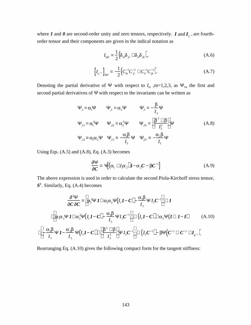
143

where 1 and 0 are second-order unity and zero tensors, respectively. I and IC −1 are fourth-

order tensor and their components are given in the indical notation as

Iijkl =12 ik jl + il jk( ), (A.6)

IC −1[ ]

ijkl= −

12

Cik−1C jl

−1 + Cil−1C jk

−1( ). (A.7)

Denoting the partial derivative of Ψ with respect to Im ,m=1,2,3, as Ψ,m the first and

second partial derivatives of Ψ with respect to the invariants can be written as

Ψ,1 = 1Ψ Ψ,2 = 2Ψ Ψ,3 = −I3

Ψ

Ψ,11 = 12Ψ Ψ,22 = 2

2Ψ Ψ,33 =2 +I3

2

Ψ

Ψ,12 = 1 2Ψ Ψ,13 = − 1

I3

Ψ Ψ,23 = − 2

I3

Ψ

(A.8)

Using Eqs. (A.5) and (A.8), Eq. (A.3) becomes

∂Ψ∂C

= Ψ 1 + I1 2( ) 1− 2C − C−1[ ] (A.9)

The above expression is used in order to calculate the second Piola-Kirchoff stress tensor,

SE. Similarly, Eq. (A.4) becomes

∂ 2Ψ∂C ∂C

= 12Ψ 1+ 1 2Ψ I11− C( ) − 1

I3

Ψ I3C−1

⊗ 1

+ 1 2Ψ 1+ 22Ψ I1 1− C( ) − 2

I3

Ψ I3C−1

⊗ I11− C( ) + 2Ψ 1⊗ 1− I( )

+ − 1

I3

Ψ 1− 2

I3

Ψ I11− C( ) +2 +I3

2

Ψ I3C

−1

⊗ I3C−1( ) − Ψ C−1 ⊗ C−1 + I

C −1( )

(A.10)

Rearranging Eq. (A.10) gives the following compact form for the tangent stiffness:

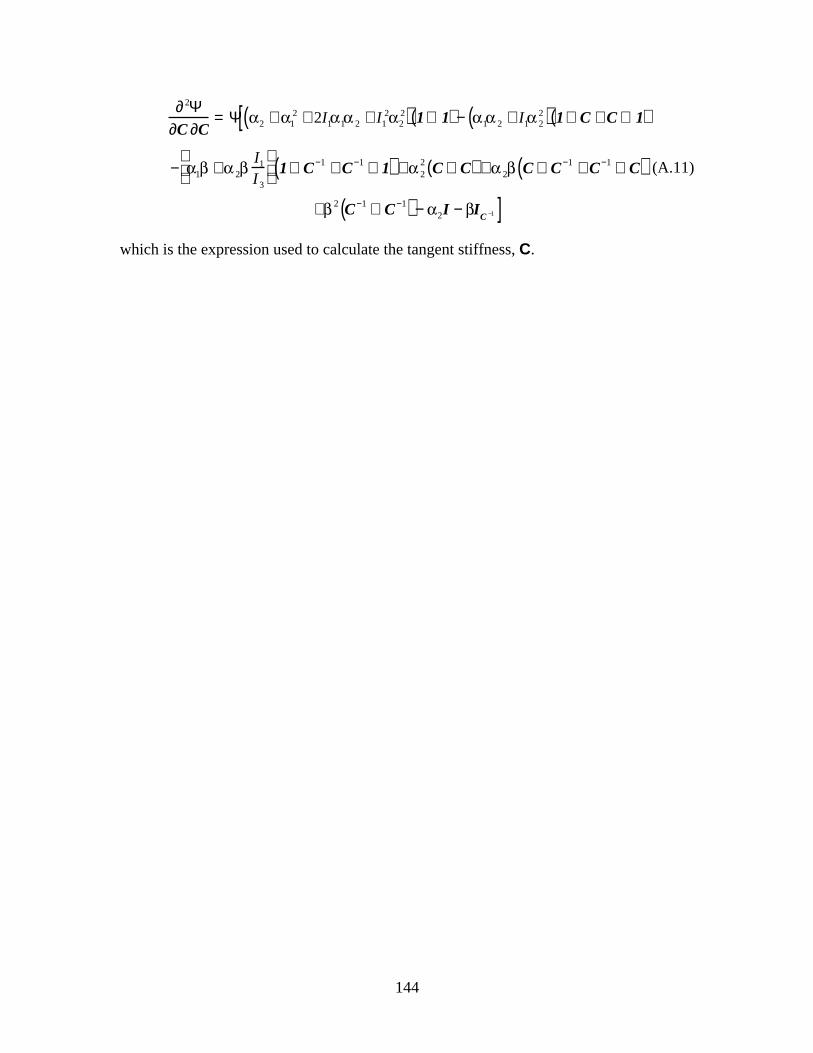
144

∂ 2Ψ∂C ∂C

= Ψ 2 + 12 + 2I1 1 2 + I1

222( ) 1⊗ 1( ) − 1 2 + I1 2

2( ) 1⊗ C + C ⊗ 1( )[

− 1 + 2

I1

I3

1⊗ C−1 + C−1 ⊗ 1( ) + 2

2 C ⊗ C( ) + 2 C ⊗ C−1 + C−1 ⊗ C( )

+ 2 C−1 ⊗ C−1( ) − 2I − IC −1 ]

(A.11)

which is the expression used to calculate the tangent stiffness, C.

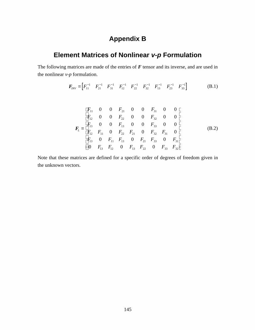
145

Appendix B

Element Matrices of Nonlinear v-p Formulation

The following matrices are made of the entries of F tensor and its inverse, and are used in

the nonlinear v-p formulation.

FINV = F11−1 F21

−1 F31−1 F12

−1 F22−1 F32

−1 F13−1 F23

−1 F33−1[ ] (B.1)

FL =

F11 0 0 F21 0 0 F31 0 0

F12 0 0 F22 0 0 F32 0 0

F13 0 0 F13 0 0 F33 0 0

F12 F11 0 F22 F21 0 F32 F31 0

F13 0 F11 F13 0 F21 F33 0 F31

0 F13 F12 0 F13 F22 0 F33 F32

(B.2)

Note that these matrices are defined for a specific order of degrees of freedom given in

the unknown vectors.

146

Appendix C

Justification for Disregarding the Tissue CurvatureEffect in Penetration Analysis

Typical tissue layers in the musculoskeletal system have curved faces. Assigning

a displacement at each point that is normal to the surface, as done in the penetration

method, will cause a corresponding tangential displacement. Here we demonstrate that

the associated tangential strains are small compared to the normal strain and can be

neglected in the elastic traction calculation in the pre-processing step. In the case of a flat

surface the analysis is similar.

Figure C.1: The penetration distribution assigned to a curved surface where g denotes

the varying penetration field and R is the radius of curvature. Line segment of length d

takes the length d’ after penetration is applied.

Consider a distribution of penetration vectors that is normal to a surface of

curvature R, Fig. C1. For simplicity let R be constant. Considering a small angle, denoted

as , a line segment of length d takes the length d' after the penetration field g deforms

the surface. It is clear that d = R and the cosine law gives

d'2 = (R − g)2 + (R − g − g)2 − 2(R − g)(R − g − g)cos( ) (C.1)

For a small angle ,

1− cos( ) ≈( )2

2(C.2)

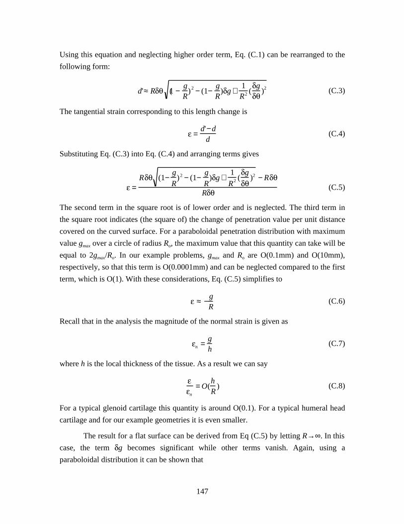
147

Using this equation and neglecting higher order term, Eq. (C.1) can be rearranged to the

following form:

d'≈ R (1 −gR

)2 − (1−gR

) g +1R2 (

g)2 (C.3)

The tangential strain corresponding to this length change is

=d'−d

d(C.4)

Substituting Eq. (C.3) into Eq. (C.4) and arranging terms gives

=R (1−

g

R)2 − (1−

g

R) g +

1

R2 (g

)2 − R

R(C.5)

The second term in the square root is of lower order and is neglected. The third term in

the square root indicates (the square of) the change of penetration value per unit distance

covered on the curved surface. For a paraboloidal penetration distribution with maximum

value gmax over a circle of radius Ro, the maximum value that this quantity can take will be

equal to 2gmax/Ro. In our example problems, gmax and Ro are O(0.1mm) and O(10mm),

respectively, so that this term is O(0.0001mm) and can be neglected compared to the first

term, which is O(1). With these considerations, Eq. (C.5) simplifies to

≈ −gR

(C.6)

Recall that in the analysis the magnitude of the normal strain is given as

n =gh

(C.7)

where h is the local thickness of the tissue. As a result we can say

n

= O(hR

) (C.8)

For a typical glenoid cartilage this quantity is around O(0.1). For a typical humeral head

cartilage and for our example geometries it is even smaller.

The result for a flat surface can be derived from Eq (C.5) by letting R→∞. In this

case, the term g becomes significant while other terms vanish. Again, using a

paraboloidal distribution it can be shown that

148

n

= O(hgmax

R02 ) (C.9)

which is O(0.001) for our example problems. For physiological problems the ratio can

have a higher order but is still negligible. The contribution of these in-plane strains to

normal elastic traction on the surface is further diminished since they multiply smaller

material coefficients (off-diagonal) in the stress-strain relation for typical isotropic and

transversely isotropic soft tissue.

Documents

A Penetration-Based Finite Element Method for Hyperelastic