Financing Development Stage Biotechnology Companies: RMs vs

Financing Development Stage Biotechnology Companies:

Reverse Mergers vs. IPOs

Mark J. Ahn, Robert B. Couch, and Wei Wu1

1 Mark J. Ahn, PhD, Associate Professor of Global Management at Atkinson Graduate School of Management, Willamette University. He can be reached at [email protected].

Robert B. Couch, PhD, Assistant Professor of Finance Atkinson Graduate School of Management, Willamette University. He can be reached at [email protected].

Wei Wu, PhD, Assistant Professor of Finance Atkinson Graduate School of Management, Willamette University. He can be reached at [email protected]. Tel: 503-370-6227. Fax: 503-370-3011.

mailto:[email protected]



2

Abstract

We examine reverse mergers (RMs) in the biotechnology industry and find that, when compared to initial public offerings (IPOs), RMs are smaller, have significantly lower market valuations relative to size, and generally invest less. We also find that RMs exhibit positive abnormal returns on the announcement date and throughout the first year after the RM event. In looking at liquidity measures, we find that RMs tend to be less liquid than IPOs and that illiquidity is greater during the six-month lock-up period following the RM event. Thus, RMs may be an appropriate alternative financing vehicle in capital intensive, high-risk biotechnology companies which require accessing deeper and larger pools of investors in public capital markets across multiple milestone periods in a “pay for progress” environment.

Key words: biotechnology, reverse merger (RM), initial public offering (IPO).

3

1. Introduction

Understanding the process by which disruptive technology platforms access capital and achieve

increasing returns to scale is critical in high technology industries generally1 and in biotechnology

specifically2 due to the degree valuation relies on intangible assets and human capital. Disruptive

technologies from emerging companies hold great promise to exploit innovation, accelerate growth, and

create value.3 However, disruptive technology platforms often face significant legitimacy hurdles due to

their small size and liability of newness, as well as their relative lack of power when it comes to multiple

stakeholder claims, control over resource flows, and business partner relationships.4

While the liability of newness is a factor for all new ventures, it is exacerbated for firms in emerging

industries created around new technologies.5 As such, organizations in emerging industries at the frontiers

of biotechnology development have to learn new roles with limited precedent for their actions, and they

must educate the broader community to establish ties in an environment that may not fully understand or

value their existence while simultaneously accessing financing. Moreover, the type of financing

approaches chosen by biotechnology firms was found to impact survival rates6 and have a “differential

impact on speed to market, control of direction, degree of technological risk, and capability

development.”7 This study explores two alternative public financing approaches, RMs (reverse mergers)

versus IPOs (initial public offerings), for development stage biotechnology companies which require

access to successively larger and deeper pools of capital to conduct advanced clinical development and

establish commercialization capabilities.

The rest of this article is organized as follows. First, we offer a more detailed discussion of the

biotechnology sector, focusing specifically on the current financial landscape. Next, we characterize our

data sample and sources. Then we analyze the financial characteristics of biotech RMs relative to biotech

IPOs and analyze the abnormal return characteristics of biotech RMs, again comparing them to biotech

IPOs. Finally, we consider liquidity measures of biotech RMs around the announcement date and the RM

event date, and around the IPO issue date.

4

2. Financial Challenges in Biotechnology

Biotechnology can be defined as “the use of cellular and biomolecular processes to solve problems or

make useful products.”8 Human therapeutics has been the largest segment of the biotech industry. The US

Food and Drug Administration (FDA) approved the first biotechnology drug in 1982. Since then, the

biopharmaceutical industry has had 254 drugs approved for 385 indications, with over $70 billion in sales

in 2007. Further, another 400 drugs targeting over 200 diseases, including various cancers, heart disease,

AIDS, and arthritis, are in clinical development, attracting over $24.8 billion in financing. As fully

integrated biotechnology giants such as Genentech, Amgen, and Biogen-Idec have emerged, the market

valuation of the biotechnology industry has recently surpassed pharmaceutical firms.

In 2009, the net income of publicly traded biotechnology companies in the United States reached an

unprecedented $3.7 billion, a dramatic increase from $400 million in 2008.9 In addition, the

biotechnology industry is an important source of new venture creation with 692 publicly listed firms in

North America, Europe, and Asia-Pacific.10 In 2008, bioscience research and development (R&D) totaled

nearly $32 billion, which accounted for more than 60 percent of all US academic R&D expenditures.

Additionally, while the private sector experienced a 3.5 percent increase in employment from 2001 to

2008, employment in the bioscience sector increased 15.8 percent.

Despite this tremendous investment, productivity over the years has been decreasing, with higher

costs of drug research and longer clinical development timelines. The average drug takes over $1.0 billion

and 12 years to go from laboratory to approval. Part of the reason for rising development costs is the high

failure rate of product candidates in clinical trials due to increasingly specific molecular targets for unmet

diseases—which necessarily increases development risk, complexity of biologic systems with

compensating mechanisms, overlapping intellectual property claims, and shifting regulatory requirements.

For the drug candidates that progress from animal testing into human clinical trials, the overall success

rate is 11 percent. In other words, nearly nine out of every ten products entering clinical trials will fail,

and some disease areas are proving to be even more challenging, for instance, oncology success rates are

5

approximately 5 percent. Furthermore, getting approval is no guarantee of commercial success. To date,

only four of ten products that reach the market achieve profitability. This lack of development

productivity (either increasing the value created or decreasing the time required to create value) has taken

its toll on industry financial performance. Out of the nearly 350 publicly traded biopharmaceutical

companies, only a small minority have reached sustainable profitability. The heavily regulated, high

complexity biopharmaceutical environment characterized by binary risk, disproportionately impacts the

sustainability of start-ups.11

Notwithstanding, a critical and somewhat unique feature of the biotech industry is the significant

amount of value that can be generated during various phases of product development that is reflected in

the ability of start-up companies to raise successive rounds of private and public capital prior to achieving

sales or net income. Significant value can be created in terms of successive private rounds of financing at

increasing enterprise valuations, obtaining liquidity by accessing public capital markets (e.g., IPOs,

RMs), as well as by executing trade sales and alliances with larger biopharmaceutical companies years

before realizing sales and profitability. In this context, development stage biotech firms represent real

options—defined as the right but not the obligation to make a series of business decisions (e.g.,

incrementally invest to advance a drug candidate from Phase II to Phase III clinical trials) by investors

and/or strategic alliance partners.12

The irregular nature of biotechnology financial markets, often characterized as “financing windows,”

increases operating risk and uncertainty (e.g., IPOs not being effective during a general market

downturn).13 As a result of large capital requirements, long lead times, and episodic successes and

failures, biotech financing cycles have been characterized by periods of high euphoria, only to be

followed by deep disillusionment after a cluster of high-profile product failures occur. This subjects early

stage companies to high degrees of financing risks, regardless of their operational progress. While the

industry has matured, the predominant venture capital financing model—one product platform or one

product, a few investors who provide seed capital, and a long incubation period leading to sale or an

6

IPO—has not markedly changed, despite reduced numbers of exits and modest overall risk-adjusted rates

of return.14

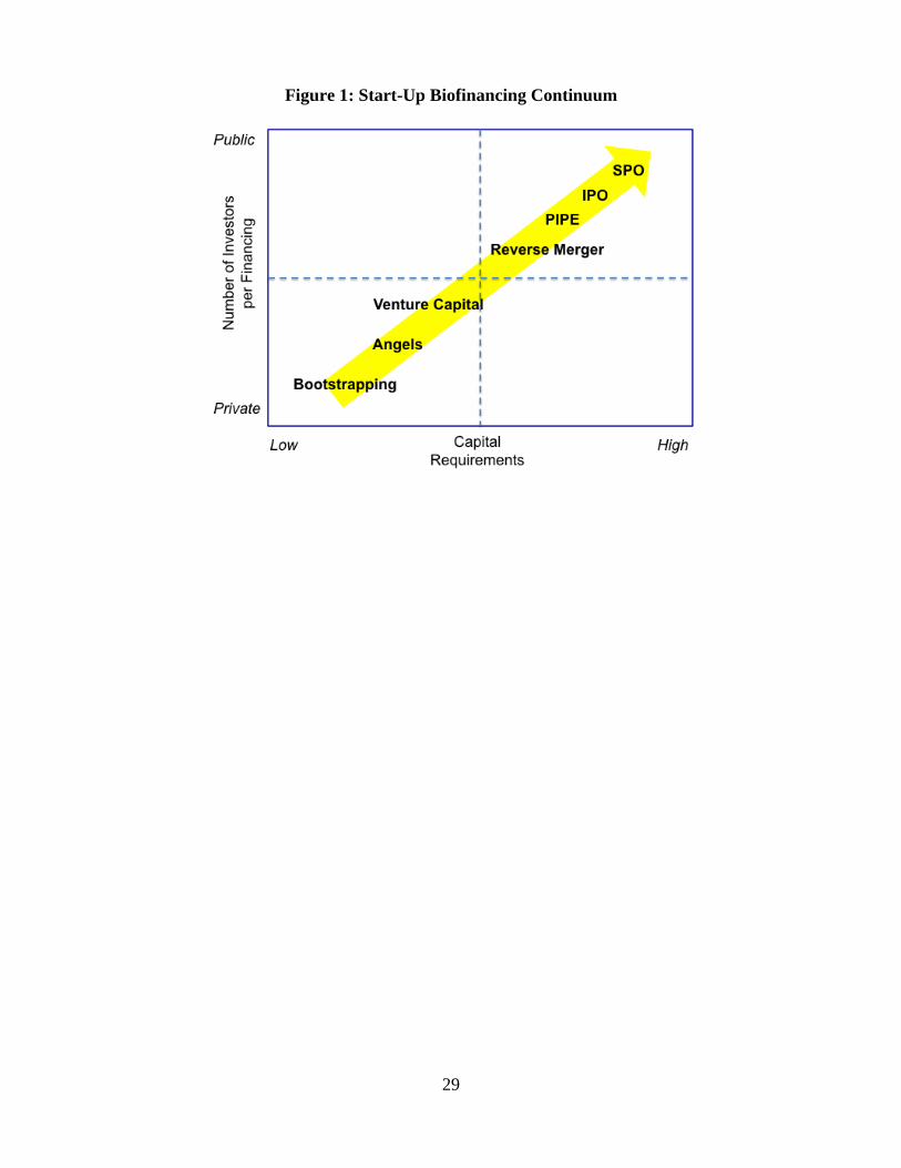
Financing approaches to biotechnology financing can be broadly categorized into private and public

financing (see Figure 1). In biotechnology, private financing sources are typically derived from academia

(e.g., majority of initial new drug (IND) applications to the FDA are from universities and research

institutes), angel investors (e.g., wealthy individuals and groups), and venture capital (e.g., pools of

private equity funds that establish limited partnerships to invest in early stage, high technology

companies). Private equity is typically seen as required in early stages of company development due to

information asymmetry between management and shareholders, such that more active governance (e.g.,

venture capital acquires board of director seats and places restrictions on capital deployment) is required.

----------------------------------------- Figure 1 about here

-----------------------------------------

Public financing, on the other hand, is achieved by selling newly issued shares in a publicly traded

company to individual and institutional investors (e.g., mutual funds, hedge funds). There are two

pathways for private biotechnology companies to obtain a public share listing to enable trading liquidity,

and access to larger and deeper pools of financing: IPOs and RMs . IPOs are the initial sale of stock that

transforms a private company into a public company with financial disclosures and filings as required by

the US Securities Exchange Act of 1934.

While biotech IPOs are open to a small number of firms that can achieve successive rounds of venture

capital and justify the large underwriting costs of investment banks, development stage R&D firms have

also proven to be difficult to price and volatile15 despite investment syndicates, strategic alliances, or

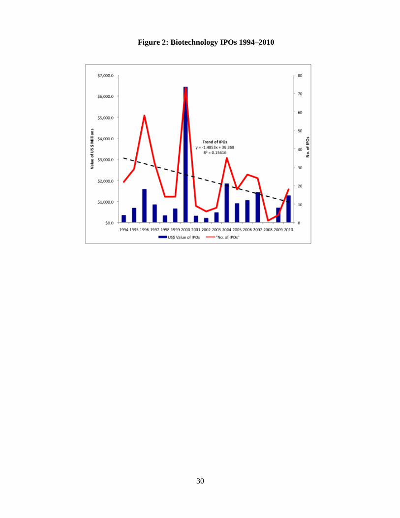
other signaling mechanisms.16 From 2006 through 2010, for example, there were 58 biotechnology IPOs

with an average pre-money valuation of $269.0 MM, an average financing of $102.1 MM, and returned -

24 percent.17 As a result, the number of IPOs has been on a steady downward trend (see Figure 2). As an

7

example of the “financing window” effect, consider Boston-based BG Medicine, a developer of

molecular diagnostics based on biomarkers, with a focus on cardiovascular, central nervous system, and

autoimmune indications, which filed for an IPO in August 2007 to raise $80 million at $13 to $15 per

share, but withdrew the proposal in January 2008 citing market conditions. The company subsequently

amended its IPO in January 2011 to raise $33.3 million shares at $7 per share.


-----------------------------------------

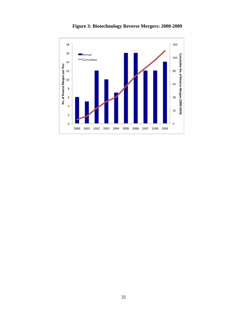
A Reverse Merger (RM) occurs when a public company purchases a private company but the private

company becomes the controlling entity after the transaction. RMs are another way a private company

may achieve a public listing and have increased popularity (see Figure 3). The publicly traded company is

called a “shell” since it has little or no business operations and derives its value with its organizational

structure. RMs are often completed at far lower valuations compared to IPOs and may be seen as

alternatives to being “priced out” by investment bank underwriters who require larger transaction sizes to

justify their efforts. RMs are also often cited as a means to avoid the costly and lengthy process of an IPO,

which includes stringent requirements imposed by the Sarbanes-Oxley Act of 2002, with studies finding

RMs costing $200,000 to $300,000 and two to 12 months less than an IPO.18 Once public, companies can

subsequently access wider and deeper pools of investors such as individuals, hedge funds, and mutual

funds.


-----------------------------------------

An example of a firm using an RM to gain access to liquidity early in its research and development

life cycle was Cougar Biotechnology (CB). In 2003, CB was formed to license early stage technologies

from Biotechnology General (BTG) and Emory University. In 2005, the private company simultaneously

obtained a convertible bridge financing of $6.1 million, which was converted into common stock after

completing an RM to obtain an over-the-counter (OTC) exchange listing. In 2005, CB used the proceeds

8

to conduct Ph I/II human clinical trials of abiraterone acetate. Based on successful clinical results, the

company completed a $50 million financing via a private placement or PIPE (private investment in public

equity). In June 2007, CB reported promising interim Ph II clinical data. In December 2007, the company

raised an additional $87 million through another PIPE financing. In April 2008, CB commenced its

registration-seeking Ph III clinical trials in metastatic, castration resistant prostate cancer in patients who

progressed after docetaxel-based chemotherapy failed, under an SPA (special protocol assessment)

approved by the US FDA. During the Phase III clinical trial, Johnson & Johnson acquired CB for $1.0

billion in a cash tender offer in May 2009.

Notwithstanding the above successful example of CB, however, studies have found mixed overall

performance results when comparing RMs to IPOs—with some showing higher,19 some neutral,20 and

some lower abnormal returns.21 As such, our research seeks to explore the role of RMs versus IPOs in the

context of the high risk, development stage, biotechnology industry sector. While RMs seem to be

increasing in popularity in the biotech sector, existing research has not examined the utility and

performance of biotech RMs as a means for expanding industry growth opportunities for early stage

companies who access successive rounds of capital in a “pay for progress” environment.22 Further,

besides shedding light on how RMs play a role in the biotech industry, our aim is to learn from the

biotech industry about the processes and challenges of raising capital to finance innovative research in a

context that entails significant long-term risks, which are difficult to monitor.

3. Data

Our sample of biotech RMs is drawn from two sources, the Securities Data Corporation’s (SDC’s)

International Mergers and Acquisition database and Windhover’s strategic transaction database. The

comprehensive data offered by SDC cover mergers and acquisitions (M&As) while the Windhover data

are specialized in alliances, financings, and M&As across biopharmaceuticals, devices, diagnostics, and

tech transfers. The SDC database incorrectly categorizes “rollups” and other forms of industry

consolidation as RMs, and improperly categorizes many ordinary IPOs and M&As between public

9

companies as RMs. Windhover, on the other hand, does not remove the deals that have withdrawn after

the initial announcement. As a result, we cross validate our sample selection using both databases.

Our final sample of biotech RMs is filtered based on the following criteria: (1) firms have Standard

Industrial Classification (SIC) codes of 2833–2836 and 8731–8733; (2) the deal synopsis in SDC or the

deal headline in Windhover clearly indentifies the deal as a RM; (3) the deal is between a private

company based in the US and a public firm listed on a U.S. stock exchange; (4) the deal has both an

announcement date and an RM even date, and it must be completed between 1/1/2000 and 12/31/2009;

(5) firm-specific financial information is available from Compustat; (6) stock-related information is

available from Center for Research in Security Prices (CRSP). The imposition of these criteria leaves us

with a total of 29 RMs from 2000 to 2009.

We compare biotech RMs with biotech IPOs. Biotech IPO data are taken from SDC’s Global New

Issues database. This sample is filtered based on the following criteria: (1) the offering companies must

have SIC codes of 2833–2836 and 8731–8733; (2) the offering is by a U.S.-based private company on a

US-based exchange; (3) the offering is not a roll-up IPO; (4) financial information is available from

Compustat; (5) stock-related information is available from CRSP. The imposition of these criteria leaves

us with a total of 137 biotech IPOs form 2000 to 2009.

We do not include financial data on private companies prior to the time that they go public via RMs

as the data are not reliable and very sparse in the databases. Instead, we collect the financials and conduct

market value calculations based on the most adjacent annual report day following the RM event date and

the issue date for IPOs.

4. Financial Characteristics of Biotech RMs

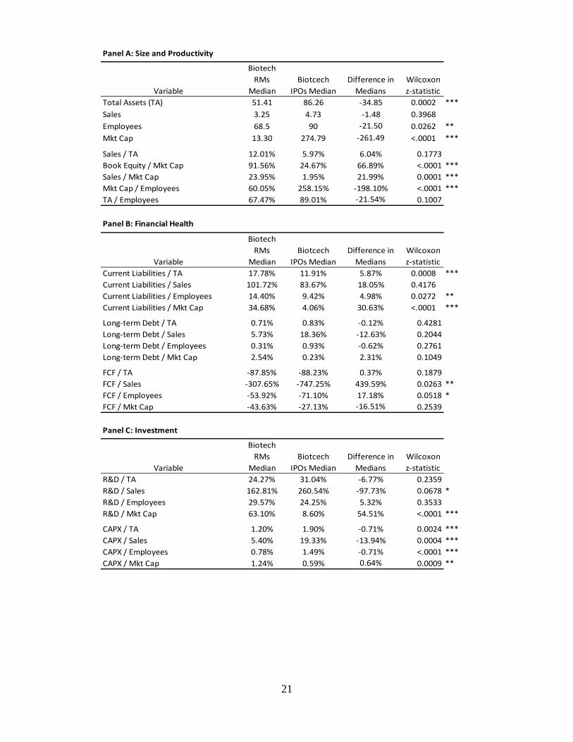
In Table 1 we compare biotech RMs with biotech IPOs. Because of the skewed nature of many of the

non-return variables, we do an analysis of medians rather than focusing on means, as is common in IPO

studies. To test for statistical significance regarding the difference between RM and IPO medians, we use

the Wilcoxon two-sample median z-test.

10

In Panel A, we look at various measures of size. The first two that we look at are total assets (TA) and

sales, since these are the two most common measures of size in financial studies. Since young biotech

firms seldom have significant sales revenue, and since the amount of measurable real assets is typically

quite small and non-representative of the real value of the firm, these measures are very noisy measures of

size. Because of this, we look at two other size measures: number of employees and market capitalization

(Mkt Cap). Number of employees is a measure that captures the current size of the firm whereas Mkt Cap

is a measure of the market’s expectations related to the expected future potential of the size and value of

the firm. In the remaining panels of Table 1, we use these four measures of size as scaling variables for

alternative firm measures aimed at capturing the financial health, investment, and growth aspects of our

sample of firms.

4.A. Size and Productivity

As measured by TA, employees and Mkt Cap, RMs are significantly smaller than IPOs (see Table 1,

Panel A). As measured by sales, the difference is not statistically significant. These results are consistent

with our expectations since the relative cost of going through the IPO process is larger for smaller firms

than larger firms.

The difference in size is most pronounced when measured by Mkt Cap, where IPOs are nearly 20

times as large as RMs. In contrast, the number of employees in IPO firms is only about 30 percent larger

than RM firms; sales are 46 percent larger and TA are 68 percent larger for IPO firms than RM firms.

This highlights the degree to which tangible measures of size (TA, sales, and employees) are measuring

only the tip of the iceberg with respect to actual, market value. The most obvious difference between RMs

and IPOs is the difference in the way the market values them. This point will be explored in more depth

below.

Looking at sales divided by TA, we find that more sales are generated for RMs than IPOs, but the

difference is not significant. Moreover, both sales and TA are likely very noisy measures of biotech firm

11

value, health, and potential, so it would be hard to draw strong inferences from this ratio anyway.

Looking at book equity divided by Mkt Cap, we find that RMs have a higher ratio than IPOs. This

corroborates our interpretation above that RMs generally receive lower valuations by the market than

IPOs, when scaled by accounting measures of firm size. Looking at sales as a percentage of Mkt Cap, we

find a similar result, presumably for similar reasons: RMs either have less access to growth financing, or

less strategic reason to grow as fast as IPOs. When we look at capital expenditures (CAPX) scaled by Mkt

Cap, we find the opposite result, that RMs have more relative CAPX than IPOs. This result is probably

best interpreted in terms of the valuation effect discussed previously: market valuations per dollar

invested are lower for RMs than for IPOs since RMs have not gone through the same vetting process of

IPO book-building and hence entail more operational and liquidity risk.

Looking at Mkt Cap scaled by the number of employees, we find that RMs have lower valuations per

employee. This suggests, again, that IPO firms have greater value and growth potential than RM firms, as

reflected in investor confidence and interest.

Looking at TA divided by number of employees, we find that RMs have fewer assets per employee.

This suggests that RM employees have less access to capital, and perhaps technology, than IPO

employees. Interestingly, this raises a question regarding the chicken or the egg: does higher valuation,

and higher expected valuations, lead firms to accumulate more assets per employee; or, does greater

assets per employee lead to higher valuations? Unfortunately, our data are not able to speak to this

question, though our hunch is that although both effects feed off each other, greater asset investment per

employee is probably a result of more promising technological development and potential.

4.B. Financial Health

Looking at current liabilities, we find that RM firms have significantly more current liabilities than

IPO firms when scaled by TA, employees, and Mkt Cap, as shown in Panel B of Table 1. The difference

is not statistically significant when current liabilities are scaled by sales. This suggests RMs are more

12

credit-constrained than IPOs.

Looking at long-term debt, we find that, relative to IPOs, RMs hold less debt relative to TA, sales,

and employees, although the difference is not statistically significant. When scaled by Mkt Cap, however,

RMs are actually shown to have more debt than IPOs, though this difference is only marginally

significant (p-value = 0.105). We interpret this result as an indication that IPOs have greater debt

capacity, but this greater debt capacity is strongly correlated with the same factors driving the high

relative valuations of IPOs.

Looking at free cash flow, we find that RMs tend to have greater relative free cash flows than IPOs

when using non-market scaling variables. This is consistent with the manner in which young biotech

firms are primarily in the game of investing in research and development of products that have only future

value rather than an ability to generate current cash flow. Thus, it seems that IPOs have a greater capacity

to incur negative free cash flows than RMs. This is likely an indication of strategic investment rather than

an indication of a deeper problem, as negative free cash flow is frequently indicative of larger, mature

firms, or firms in other industries.

4.C. Investment

Looking at research and development (R&D) expenses, we find that when R&D is scaled by sales,

the ratio is smaller for RMs than for IPOs, as shown in Panel C of Table 1. However, when scaled by Mkt

Cap, RMs are found to invest more in R&D than IPOs. These results suggest that the market valuation

multiplier that IPOs experience relative to RMs is not driven solely by R&D expenses. In other words,

since R&D measures tend to be higher for IPOs than RMs when non-market scaling variables are used,

IPOs invest relatively more in R&D than RMs; however, since the ratio of R&D to Mkt Cap is

significantly lower for IPOs than for RMs, market valuations must be driven by more than just the

differential in R&D.

Looking at CAPX, we find results that are similar to R&D: RMs are found to invest less than IPOs

13

when scaled my non-market variables, and more when scaled by Mkt Cap, and these differences are all

statistically significant at the one percent level. This result is consistent with the idea that markets are

more optimistic about IPO growth and value prospects, though the value effect is stronger than a pure

investment-growth effect.

5. Abnormal Returns

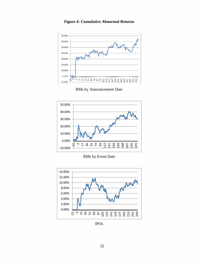
In Table 2, we show cumulative abnormal returns (CARs), net the CRSP value-weighted index, for

biotech RMs and biotech IPOs. For biotech RMs, we consider returns around the both the RM

announcement date (Panel A) and event date (Panel B), which is the effective date that the RM occurs.

IPOs are considered in Panel C. Figure 4 shows how CARs behave on a daily basis around the RM

announcement and event dates, and after the going-public issue date for IPOs.


-----------------------------------------

5.A. RM Announcement Date

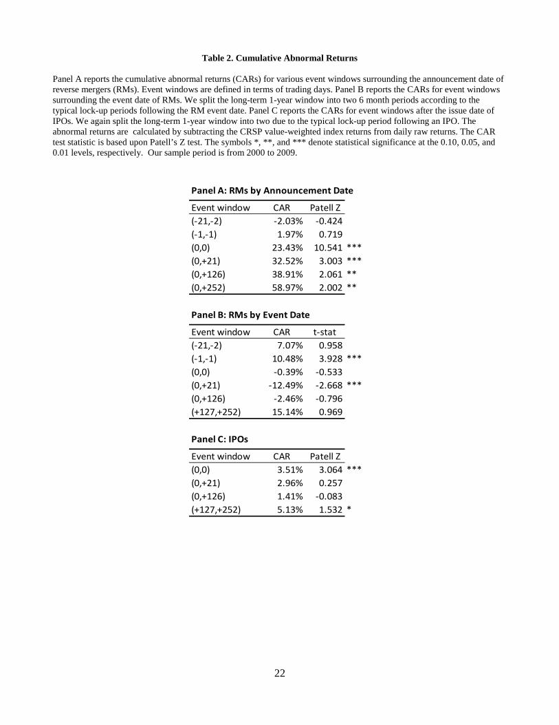
Prior to the announcement date, we do not find significant CARs, as shown in Panel A of Table 2. On

the announcement date, we find a statistically significant mean CAR of 23 percent. During the first

month, or 21 trading days, after the announcement, we find mean CARs of 33 percent, which represents

an additional CAR of 10 percent after the first day announcement day return. Over the first six months

after the announcement day, or 126 trading days, mean CARs increase slightly to 39 percent. Over the

first 12 months, or 252 trading days, mean CARs increase an additional 20 percent to 59 percent. All of

these means for CARs are statistically significant, although the first day and first month returns are

significant at the one percent level whereas the other returns are only significant at the 5 percent level.

5.B. RM Event Date

In Panel B of Table 2, we show CARS based on the RM event date. During the month prior to the

RM event date, from 21- through 2-days prior, we find mean CARs of 7 percent, which is not statistically

14

significant. On the day prior to the event date, we find mean CARs of 11 percent, which is statistically

significant at the one percent level. Since the RM event date should already be public information on the

day before the event date, this abnormal return could reflect a positive news event regarding resolved

uncertainty as to the possibility that the RM might not actually take place. Alternatively, this abnormal

return could reflect hype surrounding the transaction, or other behavioral transactions or trading behavior

associated with the RM event.

On the event date, we find mean CARs of -0.40 percent, which is not statistically significant. During

the month after the event date, we find mean CARs of -12 percent, which is statistically significant at the

one percent level. This negative CAR could be a reversal of the run-up on the day prior to the event.

During the six-month (126 trading days) lock-up period after the RM event date, we find mean CARs

of -2 percent, which is not statistically significant. During the six months after the lock-up period, from

six months to one year after the event date, we find mean CARs of 15 percent, which is not statistically

significant.

5.C. IPO Date

Since stock prices prior to the issue date for IPOs are not publicly available, the first CAR event

window we look at for IPOs is the IPO issue date. For biotech IPOs, we find mean abnormal returns on

the first trading date of 4 percent, which is statistically significant at the one percent level. During the first

month, or 21 trading days, and during the first six months, or 126 trading days, we find that mean CARs

decreases to one percent, which is not statistically significant. However, after the typical six-month lock-

up period, we find that CARs are 5 percent, which is statistically significant at the 10 percent level.

5.D. Multivariate Regressions

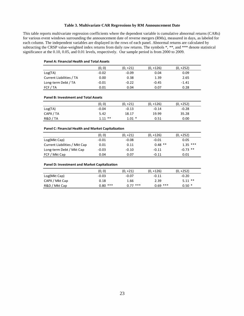
Table 3 reports multivariate regression coefficients using as the dependent variable CARs by RM

announcement date. On the day of announcement, R&D has a positive and significant coefficient when

scaled by TA and by Mkt Cap. This suggests that the market in fact anticipates that higher R&D-intensive

15

RMs should be priced higher than RMs with less R&D investment. This R&D effect remains significant

in several of the post-announcement event windows. In post-announcement event windows, current

liabilities scaled by Mkt Cap also exhibit a positive and significant effect on CARs, whereas long-term

debt scaled by Mkt Cap exhibits a negative and significant effect on one-year post-announcement CARs.

These results may reflect credit constraints with shorter-term liabilities being incurred because of lack of

good long-term financing offers, resulting in lower initial market valuations and higher subsequent

returns.

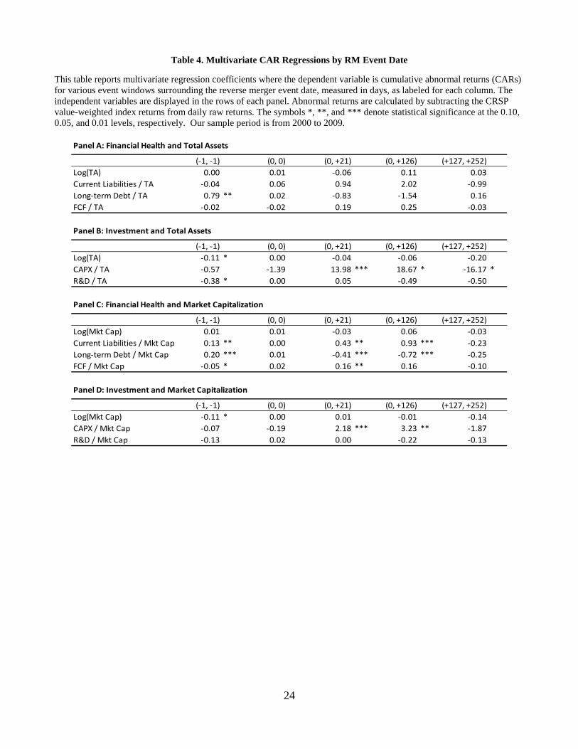
Table 4 reports multivariate regression coefficients using as the dependent variable CARs by the RM

event date. On the day prior to the RM event, both long-term debt and current liabilities have positive and

significant coefficients when scaled by Mkt Cap. This is likely due to the fact that firms with higher

liabilities effectively have a more leveraged bet on the success of the RM process being successfully

consummated, which is something that investors become significantly more confident about on the day

prior to a realized RM event. During post-event windows, current liabilities scaled by Mkt Cap continue

to have a positive and significant sign, whereas the coefficient on long-term debt scaled by Mkt Cap

becomes negative. This is the same result as was found in Figure 7 for the announcement date. Regarding

investment variables, CAPX exhibit a positive and significant effect on post-event CARs when scaled by

TA or Mkt Cap. This is similar to the result found for R&D investment in Figure 7 for the RM

announcement date, but it is curious that R&D was found to be significant in that case but CAPX was not,

and now, when looking around the RM event date, the opposite is true. The one other variable that is

statistically significant in the post-event period for RMs is free cash flow scaled by Mkt Cap. The positive

sign on this variable may be the result of a relatively short horizon in which some RM firms are

scrutinized after the RM event by investors according to their ability to generate cash flows. As will be

discussed below, this is in contrast to IPO firms.

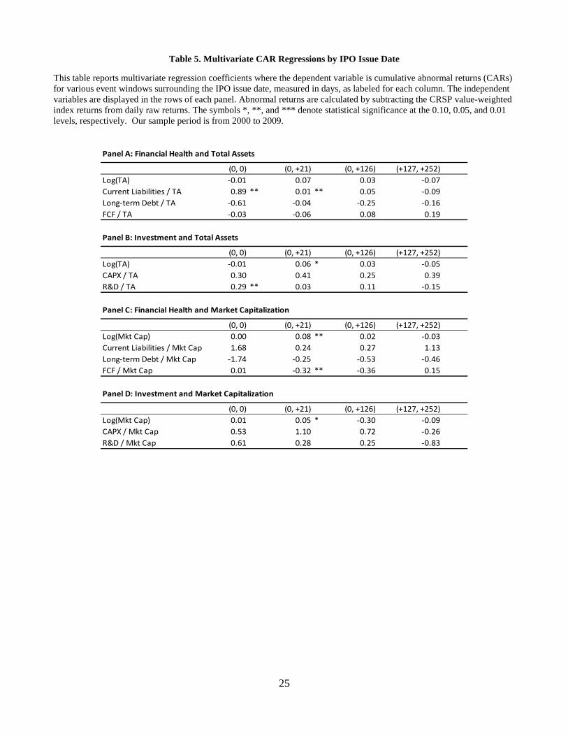
Table 5 reports multivariate regression coefficients using as the dependent variable CARs for IPO

firms by the IPO issue date. As with RMs, we find positive and significant coefficients for current

16

liabilities and R&D, both scaled by TA, in the post-event window. Like with RMs, the sign on free cash

flow scaled by Mkt Cap is statistically significant; however, in this case, the sign is negative. This could

be indicative of a longer-investment horizon associated with larger IPO firms having gone through a more

rigorously scrutinizing process of going public than RM firms. The one other statistically significant (at

the 0.05 level or higher) variable is the log of Mkt Cap which has a positive sign. This is somewhat

surprising, as size has not been found to predict abnormal returns in other IPO studies. On our

interpretation, this finding corroborates our belief regarding the relative financial advantages that large

IPO firms enjoy, and are able to exploit, in the biotech industry.

6. Liquidity

Although there are many potential sources for the relatively low valuations and subsequent high

abnormal returns documented in the previous section for biotech RMs, we focus here on the issue of

liquidity. First, we motivate and define four measures of liquidity, then we move on to statistical analysis

of these measures in our sample.

6.A. Measuring Liquidity

Based on a prior survey of empirical and theoretical liquidity asset pricing results, we use four

measures of liquidity.24 First, we construct a share turnover ratio, Turnover, by dividing the total number

of shares traded by the number of shares outstanding for a trading day and then average the daily ratios

over a sample period to have the mean share turnover ratio:

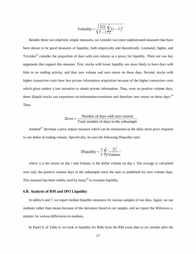
Next, we define Volatility as the standard deviation of daily returns, annualized by multiplying by the

square root of the number of trading days in a year. That is, if rt is the return on day t, and there are T

periods in the relevant subsample, and r is the average return of the relevant subsample, then

0

1 number of shares traded on day number of shares outstanding on day

T

t

tTurnoverT t=

= ∑

17

Besides these two relatively simple measures, we consider two more sophisticated measures that have

been shown to be good measures of liquidity, both empirically and theoretically. Lesmond, Ogden, and

Trzcinka25 consider the proportion of days with zero returns as a proxy for liquidity. There are two key

arguments that support this measure. First, stocks with lower liquidity are more likely to have days with

little to no trading activity, and thus zero volume and zero return on these days. Second, stocks with

higher transaction costs have less private information acquisition because of the higher transaction costs

which gives traders a low incentive to obtain private information. Thus, even on positive volume days,

these illiquid stocks can experience no-information-revelation and therefore zero return on these days.26

Thus:

Amihud27 develops a price impact measure which can be interpreted as the daily stock price response

to one dollar of trading volume. Specifically, he uses the following Illiquidity ratio:

where tr is the return on day t and Volumet is the dollar volume on day t. The average is calculated

over only the positive volume days in the subsample since the ratio is undefined for zero volume days.

This measure has been widely used by many28 to examine liquidity.

6.B. Analysis of RM and IPO Liquidity

In tables 6 and 7, we report median liquidity measures for various samples of our data. Again, we use

medians rather than means because of the skewness found in our sample, and we report the Wilcoxon z-

statistic for various differences in medians.

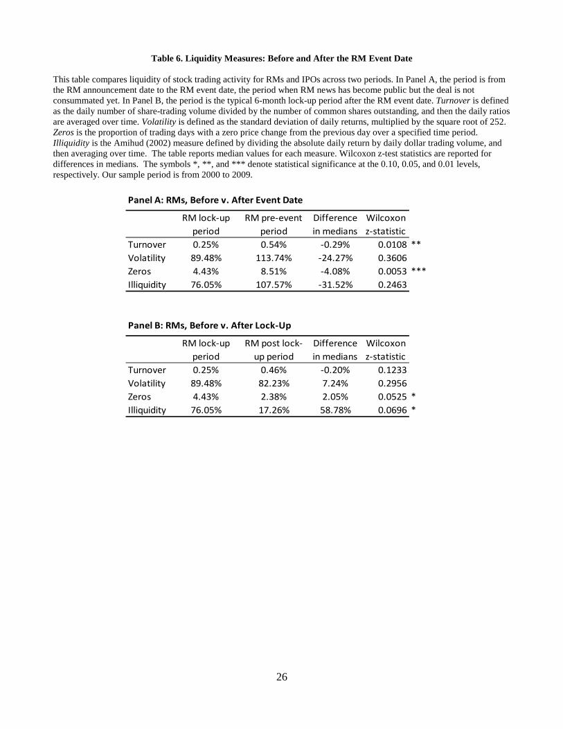
In Panel A of Table 6, we look at liquidity for RMs from the RM event date to six months after the

( )2

0

2521

T

tVolatility r r

T =

= −− ∑

Number of days with zero returnsTotal number of days in the subsample

Zeros =

0

1 Tt

t t

rIlliquidity

T Volume=

= ∑

18

event date, the “lock-up period,” and compare this sample to RMs from the RM announcement date to the

RM event date, the “pre-event period.” We find that the share turnover ratio is lower during the typical

lock-up period than during the pre-event period. This supports the idea, which will be discussed further

below, that locked-up shares form a significant portion of trading volume; thus, during the lock-up period,

trading volume is less than during other periods. We also find that Zeros is smaller during the lock-up

period relative to the pre-event period. This suggests that, although normalized trading volume is lower

during the lock-up period, the price-impact of trades is smaller. Although not statistically significant,

Volatility is also smaller during the lock-up period. Part of this result could be driven by the fact that RMs

can be withdrawn after they are initially announced.

In Panel B of Table 6, we look at liquidity for RMs for the lock-up period and compare the lock-up

period, from the RM event date through six months thereafter, to the post lock-up period, from seven

months to 12 months though 12 months after the RM event date. We find that Zeros are higher and that

Illiquidity is lower during the lock-up period than in the post lock-up period. This accords with the idea

that lock-up shares are a significant part of trading volume and that during the lock-up period price

impacts of trade are larger due to there being more asymmetric information in the market.

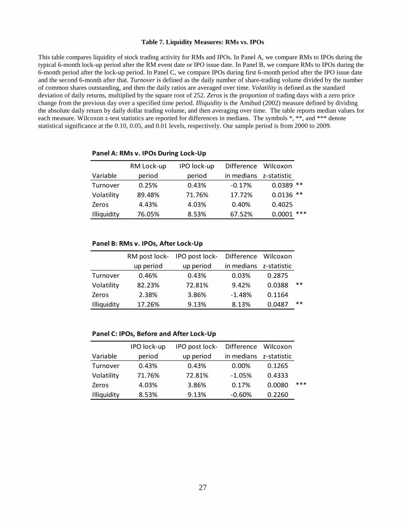
In Panel A of Figure11, we compare RMs during the lock-up period to IPOs during the lock-up

period. We find that the Turnover is lower whereas Volatility and Illiquidity are higher. IPOs tend to be

more liquid than RMs during the lock-up period, likely due to underwriter support for IPOs. Panels B and

C of Table 7 compare RMs after the lock-up period and IPOs during the six-month lock-up period to the

six-month post lock-up period, respectively. None of the differences in these comparisons is statistically

significant.

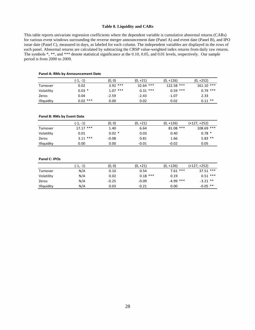
In Figure 12, we show the coefficients from univariate regressions using CAR windows for RM

announcement dates (Panel A), RM event dates (Panel B), and IPOs by issue date (Panel C) as the

dependent variable. The explanatory variable in each regression is the liquidity variable listed in each

row. Our main finding is that both Turnover and Volatility have positive and significant coefficients for

19

RMs and IPOs. Purely from the perspective of liquidity, this is somewhat puzzling, since higher turnover

indicates higher liquidity, which theoretically should be associated with a lower risk premium.29

However, these results seem consistent with the “analyst-hype” hypothesis, which predicts that successful

going-public events generate greater analyst coverage, higher turnover, and more favorable stock

returns.30 We also find that Zeros and Illiquidity have negative and significant coefficients for IPO firms,

a result that again can be interpreted as being consistent with the analyst-hype hypothesis. However, these

two variables have positive coefficients for RMs in the prior-event-day window, a result that may have

less to do with hype and more to do with liquidity risk.

7. Conclusion

We examine RMs in the biotechnology industry and find that, when compared to IPOs, RMs are

smaller, have significantly lower market valuations relative to size, and generally invest less. We also find

that RMs exhibit positive abnormal returns on the announcement date and throughout the first year after

the RM event, a result that is amplified by real firm-level investment. In looking at liquidity measures, we

find that RMs are generally less liquid than IPOs, and that illiquidity is greater during the six-month lock-

up period following the RM event. We find supporting evidence among RMs for the analyst-hype

hypothesis and a liquidity risk premium.

These findings suggest that RMs provide an important and value-increasing option for biotech firms

to access capital markets. Although investors seem to have been cautious in their initial valuations of

biotech RMs, overcoming reservations with respect to asymmetric information problems and illiquidity

risk, they have been handsomely rewarded. Thus, RMs may be an appropriate alternative financing

vehicle in capital intensive, high-risk biotechnology companies which require accessing deeper and larger

pools of investors in public capital markets across multiple milestone periods in a “pay for progress” real

options framework.

20

Table 1. Financial Characteristics This table reports median values for financial variables of reverse mergers (RMs) and initial public offerings (IPOs). The comparison focuses on size and productivity (Panel A), financial health (Panel B), and investment variables (Panel C). Free cash flow (FCF) is defined as EBIT minus taxes, plus depreciation and amortization, minus change in working capital and change in other assets. All variables except employees are in millions of dollars. All variables are measured on the most adjacent annual report day following the event date for RMs and following the issue day for IPOs. The table reports median values for each variable . Wilcoxon z-test statistics are reported for differences in medians. The symbols *, **, and *** denote statistical significance at the 0.10, 0.05, and 0.01 levels, respectively. Our sample period is from 2000 to 2009.

21

Panel A: Size and Productivity

Variable

Biotech RMs

MedianBiotcech

IPOs MedianDifference in

MediansWilcoxon z-statistic

Total Assets (TA) 51.41 86.26 -34.85 0.0002 ***Sales 3.25 4.73 -1.48 0.3968Employees 68.5 90 -21.50 0.0262 **Mkt Cap 13.30 274.79 -261.49 <.0001 ***

Sales / TA 12.01% 5.97% 6.04% 0.1773Book Equity / Mkt Cap 91.56% 24.67% 66.89% <.0001 ***Sales / Mkt Cap 23.95% 1.95% 21.99% 0.0001 ***Mkt Cap / Employees 60.05% 258.15% -198.10% <.0001 ***TA / Employees 67.47% 89.01% -21.54% 0.1007

Panel B: Financial Health

Variable

Biotech RMs

MedianBiotcech



Current Liabilities / TA 17.78% 11.91% 5.87% 0.0008 ***Current Liabilities / Sales 101.72% 83.67% 18.05% 0.4176Current Liabilities / Employees 14.40% 9.42% 4.98% 0.0272 **Current Liabilities / Mkt Cap 34.68% 4.06% 30.63% <.0001 ***

Long-term Debt / TA 0.71% 0.83% -0.12% 0.4281Long-term Debt / Sales 5.73% 18.36% -12.63% 0.2044Long-term Debt / Employees 0.31% 0.93% -0.62% 0.2761Long-term Debt / Mkt Cap 2.54% 0.23% 2.31% 0.1049

FCF / TA -87.85% -88.23% 0.37% 0.1879FCF / Sales -307.65% -747.25% 439.59% 0.0263 **FCF / Employees -53.92% -71.10% 17.18% 0.0518 *FCF / Mkt Cap -43.63% -27.13% -16.51% 0.2539

Panel C: Investment

Variable

Biotech RMs

MedianBiotcech



R&D / TA 24.27% 31.04% -6.77% 0.2359R&D / Sales 162.81% 260.54% -97.73% 0.0678 *R&D / Employees 29.57% 24.25% 5.32% 0.3533R&D / Mkt Cap 63.10% 8.60% 54.51% <.0001 ***

CAPX / TA 1.20% 1.90% -0.71% 0.0024 ***CAPX / Sales 5.40% 19.33% -13.94% 0.0004 ***CAPX / Employees 0.78% 1.49% -0.71% <.0001 ***CAPX / Mkt Cap 1.24% 0.59% 0.64% 0.0009 **

22

Table 2. Cumulative Abnormal Returns Panel A reports the cumulative abnormal returns (CARs) for various event windows surrounding the announcement date of reverse mergers (RMs). Event windows are defined in terms of trading days. Panel B reports the CARs for event windows surrounding the event date of RMs. We split the long-term 1-year window into two 6 month periods according to the typical lock-up periods following the RM event date. Panel C reports the CARs for event windows after the issue date of IPOs. We again split the long-term 1-year window into two due to the typical lock-up period following an IPO. The abnormal returns are calculated by subtracting the CRSP value-weighted index returns from daily raw returns. The CAR test statistic is based upon Patell’s Z test. The symbols *, **, and *** denote statistical significance at the 0.10, 0.05, and 0.01 levels, respectively. Our sample period is from 2000 to 2009.

Panel A: RMs by Announcement Date

Event window CAR Patell Z(-21,-2) -2.03% -0.424(-1,-1) 1.97% 0.719(0,0) 23.43% 10.541 ***(0,+21) 32.52% 3.003 ***(0,+126) 38.91% 2.061 **(0,+252) 58.97% 2.002 **

Panel B: RMs by Event Date

Event window CAR t-stat(-21,-2) 7.07% 0.958(-1,-1) 10.48% 3.928 ***(0,0) -0.39% -0.533(0,+21) -12.49% -2.668 ***(0,+126) -2.46% -0.796(+127,+252) 15.14% 0.969

Panel C: IPOs

Event window CAR Patell Z(0,0) 3.51% 3.064 ***(0,+21) 2.96% 0.257(0,+126) 1.41% -0.083(+127,+252) 5.13% 1.532 *

23

Table 3. Multivariate CAR Regressions by RM Announcement Date This table reports multivariate regression coefficients where the dependent variable is cumulative abnormal returns (CARs) for various event windows surrounding the announcement date of reverse mergers (RMs), measured in days, as labeled for each column. The independent variables are displayed in the rows of each panel. Abnormal returns are calculated by subtracting the CRSP value-weighted index returns from daily raw returns. The symbols *, **, and *** denote statistical significance at the 0.10, 0.05, and 0.01 levels, respectively. Our sample period is from 2000 to 2009.

Panel A: Financial Health and Total Assets

(0, 0) (0, +21) (0, +126) (0, +252)Log(TA) -0.02 -0.09 0.04 0.09Current Liabilities / TA 0.00 0.38 1.39 2.65Long-term Debt / TA -0.01 -0.22 -0.45 -1.41FCF / TA 0.01 0.04 0.07 0.28

Panel B: Investment and Total Assets

(0, 0) (0, +21) (0, +126) (0, +252)Log(TA) -0.04 -0.13 -0.14 -0.28CAPX / TA 5.42 18.17 19.99 35.28R&D / TA 1.11 ** 1.01 * 0.51 0.00

Panel C: Financial Health and Market Capitalization

(0, 0) (0, +21) (0, +126) (0, +252)Log(Mkt Cap) -0.01 -0.08 -0.01 0.05Current Liabilities / Mkt Cap 0.01 0.11 0.48 ** 1.35 ***Long-term Debt / Mkt Cap -0.03 -0.10 -0.11 -0.73 **FCF / Mkt Cap 0.04 0.07 -0.11 0.01

Panel D: Investment and Market Capitalization

(0, 0) (0, +21) (0, +126) (0, +252)Log(Mkt Cap) -0.03 -0.07 -0.11 -0.20CAPX / Mkt Cap 0.18 1.66 2.39 5.11 **R&D / Mkt Cap 0.80 *** 0.77 *** 0.69 *** 0.50 *

24

Table 4. Multivariate CAR Regressions by RM Event Date This table reports multivariate regression coefficients where the dependent variable is cumulative abnormal returns (CARs) for various event windows surrounding the reverse merger event date, measured in days, as labeled for each column. The independent variables are displayed in the rows of each panel. Abnormal returns are calculated by subtracting the CRSP value-weighted index returns from daily raw returns. The symbols *, **, and *** denote statistical significance at the 0.10, 0.05, and 0.01 levels, respectively. Our sample period is from 2000 to 2009.


(-1, -1) (0, 0) (0, +21) (0, +126) (+127, +252)Log(TA) 0.00 0.01 -0.06 0.11 0.03Current Liabilities / TA -0.04 0.06 0.94 2.02 -0.99Long-term Debt / TA 0.79 ** 0.02 -0.83 -1.54 0.16FCF / TA -0.02 -0.02 0.19 0.25 -0.03


(-1, -1) (0, 0) (0, +21) (0, +126) (+127, +252)Log(TA) -0.11 * 0.00 -0.04 -0.06 -0.20CAPX / TA -0.57 -1.39 13.98 *** 18.67 * -16.17 *R&D / TA -0.38 * 0.00 0.05 -0.49 -0.50


(-1, -1) (0, 0) (0, +21) (0, +126) (+127, +252)Log(Mkt Cap) 0.01 0.01 -0.03 0.06 -0.03Current Liabilities / Mkt Cap 0.13 ** 0.00 0.43 ** 0.93 *** -0.23Long-term Debt / Mkt Cap 0.20 *** 0.01 -0.41 *** -0.72 *** -0.25FCF / Mkt Cap -0.05 * 0.02 0.16 ** 0.16 -0.10


(-1, -1) (0, 0) (0, +21) (0, +126) (+127, +252)Log(Mkt Cap) -0.11 * 0.00 0.01 -0.01 -0.14CAPX / Mkt Cap -0.07 -0.19 2.18 *** 3.23 ** -1.87R&D / Mkt Cap -0.13 0.02 0.00 -0.22 -0.13

25

Table 5. Multivariate CAR Regressions by IPO Issue Date This table reports multivariate regression coefficients where the dependent variable is cumulative abnormal returns (CARs) for various event windows surrounding the IPO issue date, measured in days, as labeled for each column. The independent variables are displayed in the rows of each panel. Abnormal returns are calculated by subtracting the CRSP value-weighted index returns from daily raw returns. The symbols *, **, and *** denote statistical significance at the 0.10, 0.05, and 0.01 levels, respectively. Our sample period is from 2000 to 2009.


(0, 0) (0, +21) (0, +126) (+127, +252)Log(TA) -0.01 0.07 0.03 -0.07Current Liabilities / TA 0.89 ** 0.01 ** 0.05 -0.09Long-term Debt / TA -0.61 -0.04 -0.25 -0.16FCF / TA -0.03 -0.06 0.08 0.19


(0, 0) (0, +21) (0, +126) (+127, +252)Log(TA) -0.01 0.06 * 0.03 -0.05CAPX / TA 0.30 0.41 0.25 0.39R&D / TA 0.29 ** 0.03 0.11 -0.15


(0, 0) (0, +21) (0, +126) (+127, +252)Log(Mkt Cap) 0.00 0.08 ** 0.02 -0.03Current Liabilities / Mkt Cap 1.68 0.24 0.27 1.13Long-term Debt / Mkt Cap -1.74 -0.25 -0.53 -0.46FCF / Mkt Cap 0.01 -0.32 ** -0.36 0.15


(0, 0) (0, +21) (0, +126) (+127, +252)Log(Mkt Cap) 0.01 0.05 * -0.30 -0.09CAPX / Mkt Cap 0.53 1.10 0.72 -0.26R&D / Mkt Cap 0.61 0.28 0.25 -0.83

26

Table 6. Liquidity Measures: Before and After the RM Event Date This table compares liquidity of stock trading activity for RMs and IPOs across two periods. In Panel A, the period is from the RM announcement date to the RM event date, the period when RM news has become public but the deal is not consummated yet. In Panel B, the period is the typical 6-month lock-up period after the RM event date. Turnover is defined as the daily number of share-trading volume divided by the number of common shares outstanding, and then the daily ratios are averaged over time. Volatility is defined as the standard deviation of daily returns, multiplied by the square root of 252. Zeros is the proportion of trading days with a zero price change from the previous day over a specified time period. Illiquidity is the Amihud (2002) measure defined by dividing the absolute daily return by daily dollar trading volume, and then averaging over time. The table reports median values for each measure. Wilcoxon z-test statistics are reported for differences in medians. The symbols *, **, and *** denote statistical significance at the 0.10, 0.05, and 0.01 levels, respectively. Our sample period is from 2000 to 2009.

Panel A: RMs, Before v. After Event Date

RM lock-up period

RM pre-event period

Difference in medians

Wilcoxon z-statistic

Turnover 0.25% 0.54% -0.29% 0.0108 **Volatility 89.48% 113.74% -24.27% 0.3606Zeros 4.43% 8.51% -4.08% 0.0053 ***Illiquidity 76.05% 107.57% -31.52% 0.2463

Panel B: RMs, Before v. After Lock-Up

RM lock-up period

RM post lock-up period



Turnover 0.25% 0.46% -0.20% 0.1233Volatility 89.48% 82.23% 7.24% 0.2956Zeros 4.43% 2.38% 2.05% 0.0525 *Illiquidity 76.05% 17.26% 58.78% 0.0696 *

27

Table 7. Liquidity Measures: RMs vs. IPOs This table compares liquidity of stock trading activity for RMs and IPOs. In Panel A, we compare RMs to IPOs during the typical 6-month lock-up period after the RM event date or IPO issue date. In Panel B, we compare RMs to IPOs during the 6-month period after the lock-up period. In Panel C, we compare IPOs during first 6-month period after the IPO issue date and the second 6-month after that. Turnover is defined as the daily number of share-trading volume divided by the number of common shares outstanding, and then the daily ratios are averaged over time. Volatility is defined as the standard deviation of daily returns, multiplied by the square root of 252. Zeros is the proportion of trading days with a zero price change from the previous day over a specified time period. Illiquidity is the Amihud (2002) measure defined by dividing the absolute daily return by daily dollar trading volume, and then averaging over time. The table reports median values for each measure. Wilcoxon z-test statistics are reported for differences in medians. The symbols *, **, and *** denote statistical significance at the 0.10, 0.05, and 0.01 levels, respectively. Our sample period is from 2000 to 2009.

Panel A: RMs v. IPOs During Lock-Up

VariableRM Lock-up

periodIPO lock-up

periodDifference in medians


Turnover 0.25% 0.43% -0.17% 0.0389 **Volatility 89.48% 71.76% 17.72% 0.0136 **Zeros 4.43% 4.03% 0.40% 0.4025Illiquidity 76.05% 8.53% 67.52% 0.0001 ***

Panel B: RMs v. IPOs, After Lock-Up

RM post lock-up period

IPO post lock-up period



Turnover 0.46% 0.43% 0.03% 0.2875Volatility 82.23% 72.81% 9.42% 0.0388 **Zeros 2.38% 3.86% -1.48% 0.1164Illiquidity 17.26% 9.13% 8.13% 0.0487 **

Panel C: IPOs, Before and After Lock-Up

VariableIPO lock-up

periodIPO post lock-

up periodDifference in medians


Turnover 0.43% 0.43% 0.00% 0.1265Volatility 71.76% 72.81% -1.05% 0.4333Zeros 4.03% 3.86% 0.17% 0.0080 ***Illiquidity 8.53% 9.13% -0.60% 0.2260

28

Table 8. Liquidity and CARs

This table reports univariate regression coefficients where the dependent variable is cumulative abnormal returns (CARs) for various event windows surrounding the reverse merger announcement date (Panel A) and event date (Panel B), and IPO issue date (Panel C), measured in days, as labeled for each column. The independent variables are displayed in the rows of each panel. Abnormal returns are calculated by subtracting the CRSP value-weighted index returns from daily raw returns. The symbols *, **, and *** denote statistical significance at the 0.10, 0.05, and 0.01 levels, respectively. Our sample period is from 2000 to 2009.

Panel A: RMs by Announcement Date

(-1, -1) (0, 0) (0, +21) (0, +126) (0, +252)Turnover 0.02 3.92 *** 32.64 *** 122.58 *** 161.10 ***Volatility 0.03 * 1.07 *** 0.31 *** 0.59 *** 0.79 ***Zeros 0.04 -2.59 -2.43 -1.07 2.33Illiquidity 0.02 *** 0.00 0.02 0.02 0.11 **

Panel B: RMs by Event Date

(-1, -1) (0, 0) (0, +21) (0, +126) (+127, +252)Turnover 17.17 *** 1.40 6.64 81.08 *** 108.69 ***Volatility 0.01 0.02 * 0.03 0.40 0.78 *Zeros 3.11 *** -0.08 0.81 1.66 5.83 **Illiquidity 0.00 0.00 -0.01 -0.02 0.05

Panel C: IPOs

(-1, -1) (0, 0) (0, +21) (0, +126) (+127, +252)Turnover N/A 0.10 0.54 7.61 *** 37.51 ***Volatility N/A 0.02 0.18 *** 0.19 0.51 ***Zeros N/A -0.25 -0.09 -4.99 *** -3.21 **Illiquidity N/A 0.03 -0.21 0.00 -0.05 **

29

Figure 1: Start-Up Biofinancing Continuum

30

Figure 2: Biotechnology IPOs 1994–2010

31

Figure 3: Biotechnology Reverse Mergers: 2000-2009

32

Figure 4: Cumulative Abnormal Returns

RMs by Announcement Date

RMs by Event Date

IPOs

-10.00%

0.00%

10.00%

20.00%

30.00%

40.00%

50.00%

-21 -2 17 36 55 74 93 112

131

150

169

188

207

226

245

0.00%

2.00%

4.00%

6.00%

8.00%

10.00%

12.00%

14.00%

-21 -3 15 33 51 69 87 105

123

141

159

177

195

213

231

249

33

34

Reference

1 Christensen, C, Overdorf, M, “Meeting the Challenge of Disruptive Change,” Harvard Business Review, 78, 66–76 (2000); Brekke, OH, Sandlie, I, “Therapeutic Antibodies for Human Diseases at the Dawn of the Twenty-First Century,” Nature Review of Drug Discovery, 2, 52–62 (2003); Pera, MF, Trounson, AO, “Human Embryonic Stem Cells: Prospects for Development,” Development, 131, 5515–25 (2004); Stylios, GK, Giannoudis, PV, Wan, T, “Applications of Nanotechnologies in Medical Practice,” Injury, 36, S6–S13 (2005).

2 Zimmerman, MA, Deeds, DL, “Legitimacy and the Initial Public Offerings of Biotechnology Firms,” Frontiers for Entrepreneurship Research, 1987, available at www.babson.edu/entrep/fer/papers97; Deeds, DL, Decarolis, D, Coombs, JE, “The Impact of Firm-Specific Capabilities on the Amount of Capital Raised in an Initial Public Offering: Evidence from the Biotechnology Industry,” Journal of Business Venturing, 12, 31–46 (1997); George, G, Kotha, R, Zheng, Y “Entry into Insular Domains: A Longitudinal Study of Knowledge Structuration and Innovation in Biotechnology Firms,” Journal of Management Studies, 45, 1448–1474 (2008); Ahn, M, Davenport, S, Meeks, M, Bednarek, R “Exploring Technology Agglomeration Patterns for Multinational Pharmaceutical and Biotechnology Firms,” Journal of Commercial Biotechnology, 16: 17–32 (2009).

3 Laurie, D, Doz, Y, Sheer, C, “Creating New Growth Platforms,” Harvard Business Review, 84, 80–90 (2006).

4 Stinchcombe, AL, “Organizations and Social Structure” in March, JG (Ed.), Handbook of Organizations, Chicago: Rand-McNally (1965); Singh, J, Tucker, D, House, “Organizational Legitimacy and the Liability of Newness,” Administrative Science Quarterly, 31, 171–193 (1986); Hannan, MT, Carroll, GR, Dynamics of Organizational Populations: Density, Legitimation, and Competition, New York; Oxford: Oxford University Press (1992); Aldrich, HE, Fiol, CM “Fools Rush In? The Institutional Context of Industry Creation,” Academy of Management Review, 19, 645–670 (1994); Ruef, M, Scott, WR, “A Multidimensional Model of Organizational Legitimacy: Hospital Survival in Changing Institutional Environments,” Administrative Science Quarterly, 43(4): 877–904 (1998).

5 Aldrich, Fiol, supra, n.4.; Rao, RS, Chandy, RK, Prabhu, JC “The Fruits of Legitimacy: Why Some New Ventures Gain More from Innovation Than Others,” Journal of Marketing, 72, 58–75 (2008).

6 Morgan Jr, IW, Abetti, PA, “Private and Public ‘Cradle to Maturity’ Financing Patterns of U.S. Biotech Ventures (1970–2001),” Journal of Private Equity, Spring, 9–25 (2004); Adjei, F, Cyree, KB, Walker, MM, “The Determinants and Survival of Reverse Mergers vs IPOs,” Journal of Economics and Finance, 32, 176–194 (2008).

7 Banerjee, PM, “Financing as Mother's Milk for Internaional Biotechnology Start-Ups,” International Journal of Technoentrepreneurship, 2, 1, 45–63, p. 45 (2009).

8 BIO (Biotechnology Industry Organization), “BIO 2005–2006: Guide to biotechnology,” Washington DC: BIO (2007).

9 Ernst & Young (2006) “Beyond Borders: A Global Perspective,” EYGM Limited, available at www.ey.com.

10 Ahn, M, Meeks, M, “Building a Conducive Environment for Life Science–Based Entrepreneurship and Industry Clusters,” Journal of Commercial Biotechnology, 14, 20–30 (2007); Tufts (The Tufts Centre for the Study of Drug Development), “Structuring Clinical Organization to Improve R&D Productivity,” available at www.csdd.tufts.edu (2007).

11 Pisano, G, “Can Science Be a Business?” Harvard Business Review, 10, 1–12, (2006). 12 Kellogg, D, Charnes, JM, “Real-Options Valuation for a Biotechnology Company,” Financial Analysts

Journal, 56, 3, 76–84 (2000). 13 Deeds, DeCaolis, Coombs, supra, n.2.; Gulati, R, Higgins, MC, “Which Ties Matter When? The

Contingent Effects of Interorganizal Partnerships on IPO Success,” Strategic Management Journal, 24, 2, 127–144 (2003).

14 Pisano, supra, n.11. 15 Daily, CM, Certo, ST, Dalton, DR, Roengpitya, R, “IPO Underpricing: A Meta-Analysis and Research

Synthesis,” Entrepreneurship Theory and Practice, Spring, 271–295 (2003); Purnanandam, AK, Swaminathan,

35

B, “Are IPOs Really Underpriced?” The Review of Financial Studies, 17, 3, 811–848 (2004); Demers, E, Joos, P, “IPO Failure Risk,” Journal of Accounting Research, 45, 2, 333–372 (2007); Guo, R, Lev, B, Shi, C, “Explaining the Short- and Long-Term IPO Anomalies in he US by R&D,” Journal of Business Finance and Accounting, 33, 550–579 (2006); Pukthuanthong, K, “Underwriter Learning About Unfamiliar Firms: Evidence from the History of Biotech IPOs,” Journal of Financial Markets, 9, 366–407, (2006).

16 Gulati, Higgins, supra, n.12; Guo, R, Lev, B, Zhou, N, “Competitive Costs of Disclosure by Biotech IPOs,” Journal of Accounting Research, 42, 2, 319–355 (2004); Williams, DR, Duncan, WJ, Ginter, PM, Shewchuk, RM, “Do Governance , Equity Characteristics, and Venture Capital Involvement Affect Long-Term Wealth Creation in US Health Care and Biotechnology IPOs?” Journal of Health Care Finance, 33, 1, 54–71 (2006).

17 BMO, “Biopharma Data Tables,” BMO Capital Markets Report (2011). 18 Floros, IV, Sapp, TRA, “Shell Games: On the Value of Shell Companies,” Working Paper, available at

www.ssrn.com (2010); Feldman, D, “Reverse Mergers: Taking a Company Public Without an IPO”, Bloomberg Press, New York (2006).

19 Floros, Sapp, supra, n.18. 20 Arellano-Ostoa, A, Brusco, S, “Understanding Reverse Mergers: A First Approach,” Working Paper,

Universidad Carlos III De Madrid (2002); Gleason, KC, Rosenthal, L., Wiggins III, RA, “Backing into Being Public: An Exploratory Analysis of Reverse Takeovers,” Journal of Corporate Finance, 12, 54–79 (2005).

21 Adjei, F, Cyree, KB, Walker, MM, “The Determinants and Survival of Reverse Mergers vs. IPOs,” Journal of Economics and Finance, 32, 176–194 (2008).

22 Kellogg, Charnes, supra, n.12. 24 Chordia, T, Huh, SW, Subrahmanyam, A, “Theory-Based Illiquidity and Asset Pricing,” Review of

Financial Studies, 22, 9, 3629–3668 (2009). 25 Lesmond, D. A., J. P. Ogden, and C. A. Trzcinka, “A New Estimate of Transaction Costs,” Review of

Financial Studies, 12, 5, 1113–1141 (1999). 26 For measuring liquidity in emerging markets, the Zeros measure has been used by: Bekaert, G, Harvey,

CR, Lundblad, C, “Liquidity and Expected Returns: Lessons from Emerging Markets,” Review of Financial Studies, 20, 1783–1831 (2007); Zhang, H, “Measuring Liquidity in Emerging Markets,” National University of Singapore Working Paper.

27 Amihud, Y., “Illiquidity and Stock Returns: Cross-Section and Time Series Effects,” Journal of Financial Markets, 5, 1, 31– 56 (2002).

28 See Acharya, Viral and Lars H. Pedersen, “Asset Pricing with Liquidity Risk,” Journal of Financial Economics, 77, 2, 375– 410 (2005); Hasbrouck, Joel, “Trading Costs and Returns for U.S. Equities: Estimating Effective Costs from Daily Data,” 64, 3, 1445–1477 (2009); among others.

29 Chordia, Huh, Subrahmanyam, supra, n.24. 30 Degeorge, F, Derrian, F, Womack, K, “Analyst Hype in IPOs: Explaining the Popularity of

Bookbuilding,” Review of Financial Studies, 20, 4, 1021–1058 (2007).

Documents

Financing Development Stage Biotechnology Companies: RMs vs