Embed Size (px)
Citation preview

Master's Thesis in Mechanical/Structural
Engineering
Fatigue analysis of welded
joints in a forestry machine - Utilizing the notch stress concept
Authors: Martin Nyström, Tainan Pantano
Tomaz
Surpervisor LNU: Andreas Linderholt
Examinar, LNU: Andreas Linderholt
Surpervisor company: Mattias König, Rottne
Industri AB
Course Code: 4BY05E/4MT01E
Semester: Spring 2015, 15 credits
Linnaeus University, Faculty of Technology


III
Abstract
Welding is one of the most applied technics in the world for joining steel. Welds are
liable to the phenomenon of fatigue, which is, primarily, the formation of a crack and
consequently reduction of strength due to the action of time varying loads. Fatigue is
one of the main causes of failure in steel structures. The aim of this thesis is to do
static and dynamic analyses of a forestry crane with the purpose of using the analyses
to determine the lifetime due to fatigue of welded components.
Two methods for fatigue assessment are used in this work, the Hot-Spot Method and
the Notch Stress Method. The first boom, which is a key component for the crane, is
analyzed in a Finite Element Method (FEM) software. The found principal stress in
accordance with the notch stress method in the first boom is ±165 MPa for the
analyzed load case, rendering in a stress range of 330 MPa. The fatigue strength class
FAT-225 (m=3), leads to an expected number of 6.33 ∙ 105cycles, with a probability
of survival of 97,7% for this case.
Key words: Weld, Fatigue, Finite Element Method, Hot-Spot Method, Notch Stress
Method, Structural Dynamics, Forestry Crane

IV
Sammanfattning
Svetsning är en av de vanligaste teknikerna för sammanfogning av stål. Svetsar är
känsliga för utmattning. Utmattningsfenomenet består primärt av en initial
dislokation som genom tidsvarierande belastning formar en spricka som växer och
därmed reducerar styrkan i konstruktionen. Utmattning är en av de vanligaste
orsakerna till skador i stålkonstruktioner. Målet med detta arbete är att genomföra
både statiska och dynamiska analyser av en skogsmaskins kran i avseende att
bestämma utmattningslivslängden för dess svetsade konstruktioner.
Två metoder för utvärdering används i detta arbete, hot-spot-metoden och
notch-stress-metoden. Kranens första bom (lyftarmen) som är en huvudkomponent i
kranen analyseras med hjälp av ett Finita Element program i enlighet med
notch-metoden. Högsta funna spänningsvariationen i första
huvudspänningsriktningen var ±165 MPa för ett av de analyserade lastfallen.
Utmattningsklass FAT 225 (m=3) ger en uppskattning om utmattningslivslängd på
6,33 ∙ 105 cykler med en sannolikhet för överlevnad på 97,7% i detta fall.
Nyckelord: Svets utmattningslivslängd, Finita-elementmetoden, Hot-spot,
Notch-stress, Notch-spänning, Strukturdynamik, Skogsmaskinskran
V
Acknowledgement
A special acknowledgement is given to Rottne Industri AB; Mattias König as
supervisor and Ulf Wilhelmsson and Daniel Sätermark for giving support on the
CAD- and FEM software.
We would also like to thank our supervisor, Andreas Linderholt, for helping us
during the whole thesis.
An acknowledgement is given to CNPq (the Brazilian National Council for Scientific
and Technological Development) and CAPES (Coordination for the Improvement of
Higher Education Personnel) for providing financial support through the Brazilian
mobility program - Science without Borders.
Martin Nyström & Tainan Pantano Tomaz
Växjö, Sweden, 27th of May 2015

VI
Table of contents
1. INTRODUCTION...................................................................................................... 1
1.1 BACKGROUND ................................................................................................................................... 2 1.2 AIM AND PURPOSE ............................................................................................................................. 2 1.3 HYPOTHESIS AND DELIMITATIONS ..................................................................................................... 3
1.3.1 Hypothesis ............................................................................................................................... 3 1.3.2 Delimitations ........................................................................................................................... 3
1.4 THESIS MOTIVATION .......................................................................................................................... 4 1.5 RELIABILITY, VALIDITY AND OBJECTIVITY ........................................................................................ 5
2. THEORY .................................................................................................................... 6
2.1 FATIGUE ............................................................................................................................................ 6 2.1.1 Definition ................................................................................................................................. 6 2.1.2 The S-N diagram and Palmgren-Miner rule ........................................................................... 6 2.1.3 Approaches for fatigue assessment ......................................................................................... 8 2.1.4 Influential factors on fatigue strength ................................................................................... 10
2.2 FINITE ELEMENT METHOD ................................................................................................................ 10 2.2.1 Definition ............................................................................................................................... 10 2.2.2 1D-elasticity beam ................................................................................................................. 11 2.2.3 The notch stress method applied to FE-analysis ................................................................... 12
2.3 STRUCTURAL DYNAMICS ................................................................................................................. 13 2.3.1 Eigenvalue problem (EVP) and modal matrices ................................................................... 13 2.3.2 Modal analysis ...................................................................................................................... 14 2.3.3 State-space ............................................................................................................................ 14 2.3.4 Free vibration for a single-degree of freedom system having viscous damping ................... 15
2.4 LITERATURE REVIEW ....................................................................................................................... 17
3. METHOD ................................................................................................................. 19
3.1 CRANE SETUP .................................................................................................................................. 19 3.2 DEFINITION OF LOAD CASES............................................................................................................. 20 3.3 CALCULATION MODEL ..................................................................................................................... 20
3.3.1 Static analysis ........................................................................................................................ 25 3.3.2 Dynamic analysis .................................................................................................................. 25 3.3.3 Finite Element analysis ......................................................................................................... 26
3.4 PREDICTION OF THE LIFETIME OF THE CHOSEN WELD ....................................................................... 32 3.5 DAMPING EXPERIMENT .................................................................................................................... 33

VII
4. RESULTS ................................................................................................................. 34
4.1 STATIC ANALYSIS ............................................................................................................................ 34 4.1.1 Load case 1............................................................................................................................ 36 4.1.2 Load case 2............................................................................................................................ 36 4.1.3 Load case 3............................................................................................................................ 37 4.1.4 Load case 4............................................................................................................................ 37 4.1.5 Load case 5............................................................................................................................ 38 4.1.6 Load case 6............................................................................................................................ 38 4.1.7 Load case 7............................................................................................................................ 39
4.2 DYNAMIC ANALYSIS ........................................................................................................................ 39 4.2.1 Load case 1............................................................................................................................ 42 4.2.2 Load case 2............................................................................................................................ 43 4.2.3 Load case 3............................................................................................................................ 44 4.2.4 Load case 4............................................................................................................................ 45 4.2.5 Load case 5............................................................................................................................ 46 4.2.6 Load case 6............................................................................................................................ 47 4.2.7 Load case 7............................................................................................................................ 48
4.3 FINITE ELEMENT ANALYSIS ............................................................................................................. 49 4.3.1 First step: hot-spot stresses ................................................................................................... 49 4.3.2 Second step: notch stress method .......................................................................................... 60
4.4 FATIGUE CALCULATIONS ................................................................................................................. 61 4.5 DAMPING EXPERIMENT .................................................................................................................... 61
5. ANALYSIS ................................................................................................................... 63
6. DISCUSSION ............................................................................................................... 65
7. CONCLUSIONS .......................................................................................................... 66
REFERENCES ................................................................................................................. 67
APPENDICES .................................................................................................................. 69

1
Nyström, M; Tomaz, T. P.
1. Introduction
The forest industry is known as a particularly strong cluster in Sweden.
From the economical perspective, it provides a direct employment to around
60,000 people and in several regions it accounts for at least 20% of the
employment (Swedish Forest Industries, 2013). On a global scale, around 10
million people are employed in forest management and conservation (FAO,
2010). There is a significant progress in developing forest policies, laws and
national forest programs worldwide. Also, there is an increase in the
European recreational forest area and more than 90% of European forests
are open for public access (FAO, 2010).
The most used way to harvest trees in Sweden is through thinning and clear-
cuts in the forest using harvester machines. These harvesters can measure
and cut-to-length logs, according to the market demand (Johansson, 2011).
Rottne Industri AB is a Swedish established company, located in the region
of Småland, which produces forestry machinery, such as harvesters and
forwarders, having 50% of its production exported to other countries in
Europe and North America (Rottne Industri AB, 2014).

2
Nyström, M; Tomaz, T. P.
1.1 Background
Rottne Industri AB was founded in 1955 and has, since then, been a supplier
of equipment and vehicles for the mechanized forestry work. Rottne takes a
role during all steps of forest machines fabrication, from design until
assembling of all parts. The company has, among other functions, its own
manufacturing of welded and machined components.
Welding is one of the most applied technics in the world for joining steel
and it is being used in innumerous engineering structures. In many cases,
other types of connections (for instance fasteners) are not suitable due to the
assembling procedure or to the geometry of the steel components.
Nevertheless, the welds are liable to the phenomenon of fatigue which is a
major challenge in welding design. Fatigue is, primarily, the formation of a
crack and consequently a reduction of strength due to the action of time
varying loads (Macdonald, 2011).
Cracks generated can increase in size and lead steel components to failure
(Witek, 2009). Many researchers, for instance (Marin & Nicoletto, 2009) and
(Ritchie, 1998), consider fatigue cracking as the principal failure mode in
welds. The last states that over 80% of all service failures are related to
mechanical fatigue, e.g. cyclic plasticity, elevated temperatures (creep
failure) and environmental damage (corrosion failure).
1.2 Aim and Purpose
The aim of this thesis is to do dynamic analyses of a forestry crane with the
purpose of using the analyses for further product development and to
determine fatigue lifetime of welded components.
In addition, this thesis aims to broaden the theoretical study in this field and
specifically to transfer scientific knowledge to Rottne Industri AB for use in
their design and modeling of structures.

3
Nyström, M; Tomaz, T. P.
1.3 Hypothesis and Delimitations
1.3.1 Hypothesis
It is possible to predict the lifetime of structural components in a forestry
crane by the use of finite element analyses and weld fatigue calculations of
the structure.
1.3.2 Delimitations
Engineering is considered to be a non-exact science because most of the
time, there is no single best solution to a problem (Chow, 2002). Based on
that, many approximations and simplifications are done in order to get a
result that comprises both quality and attend deadlines.
The delimitations for this thesis are presented in Table 1.
Table 1: Delimitations.
Delimitations Comments
The welds, including the heat-
affected zone, are assumed to be
lifetime limiting
The virgin steel used for the crane has
a higher reistance to fatigue than the
welds
The boom position is set to a
predefined configuration
In normal use the crane is constantly
changing configuration. The choice of
configuration will influence the result
significantly
Only the crane’s first boom is
analysed using the finite element
software
Other components may break before
any main component does. This is,
though, less negative for the customer
both from an economical and
productivity view
Only seven load cases originated
by the combination of three
different actuators will be
considered
In normal use there are infinitely many
possible load cases

4
Nyström, M; Tomaz, T. P.
1.4 Thesis motivation
Since Rottne is interested in improving design, increasing customer value
and minimizing weight through reducing material waste, a new study on
fatigue analysis of welded steel components, lifetime prediction, and
consequent product development was suggested.
The company recently developed a new harvester named H21D , which is
equipped with a crane RK-250 with a lifting torque of 310 kNm and a total
reach of 10 m distance, see Figure 1. This crane is the object of this study on
fatigue.
A harvester can work on an average productivity of 100 trees per hour, being
subjected to cyclically varying loads and having many welded connections.
Figure 1: Harvester H21D (Rottne Industri AB, 2014)

5
Nyström, M; Tomaz, T. P.
1.5 Reliability, validity and objectivity
All the measures of the crane and its components are obtained from
brochures and 3D solid CAD models provided by the company. The same
procedure can be applied for further studies in this area.
The boom configuration is chosen to one particular case. However, the crane
has a constantly changing configuration during its operation. The
configuration used during this work is chosen to represent the normal
working range (Rottne Industri AB, 2014) and therefore has enough validity.
The finite element analyses are made on the first boom’s welds, since they
are the key components for the crane’s operation. Practice, for example the
works Mechanisms of fatigue-crack propagation in ductile and brittle solids
(Marin & Nicoletto, 2009) and Fatigue design of welded joints using the
finite element method and the 2007 ASME Div.2 Master Curve (Ritchie,
1998), have shown that welds are the most critical parts for fatigue failure.

6
Nyström, M; Tomaz, T. P.
2. Theory
This chapter presents relevant theory of Fatigue Behavior, the Finite
Element Method and Structural Dynamics modeling.
2.1 Fatigue
2.1.1 Definition
Most steel structures are liable to repeated loadings and unloadings, which
can cause microscopic cracks. After many repeated loadings and unloadings,
the cracks can increase in size and then lead the metal to failure, as shown in
Figure 2. Fatigue can also be defined as the reduced strength originated by
the formation of cracks.
Figure 2: Locations of crack propagation in welded joints (Hobbacher, 2008)
2.1.2 The S-N diagram and Palmgren-Miner rule
The pioneer of fatigue studies was August Wöhler (1819-1914), who first
established a systematic way to identify and quantify fatigue on locomotive
axles (Timoshenko, 1983).
A simplified version of one of his experiments consisted of a 4-point
bending rotational beam. After imposing several bending moments, the
number of cycles until failure is counted and plotted versus the stress
variation. From the obtained points within the stress range it is possible to
draw an approximative relation between the stress (S) and the number of
cycles (N). This is known as the S-N diagram (S for strength and N for
number of cycles); or as a Wöhler Curve, which is shown in Figure 3.

7
Nyström, M; Tomaz, T. P.
Figure 3: A typical S-N diagram – Cycles to failure (European prestandard, 2002)
Each material has its own S-N curve and is classified according to the
“FAT” grade. A characteristic curve, FAT-225 for example, has a fatigue
strength of 225 MPa at 2 million cycles for a 2,3% failure probability
(Fricke, 2007).
The S-N diagram is obtained from tests stemming from constant loadings.
However, structures are usually subjected to many loading and unloading
cycles, for which the stresses varies in a more complicated manner. In order
to take these fluctuating stresses into account, the Palmgren-Miner theorem,
which consists of a damage summation, is applied.
According to this method (Eriksson, et al., 2002), failure occurs when,
∑𝑛𝑖𝑁𝑖
𝐼
𝑖=1
= 1
( 1 )
where 𝑛𝑖 is the number of loadings with stress value 𝜎𝑖 and 𝑁i is the fatigue
life for stress 𝜎𝑖. An example of a damage accumulation problem is shown in
Appendix 2.

8
Nyström, M; Tomaz, T. P.
2.1.3 Approaches for fatigue assessment
There are several approaches for fatigue assessment of welded joints. The
most relevant, due to large industry application in recent years (Hobbacher,
2008), are the:
Nominal stress method;
Structural hot-spot stress method;
Effective notch stress method.
Other approaches, such as fracture mechanics, are not addressed in this
thesis.
2.1.3.1 The nominal stress method
The Nominal Stress approach is based on the stresses in the cross-sectional
area of the component considering the effects of particular macro-geometric
shape in the vicinity of the joint (Figure 4). Eventual local stresses are
excluded (Hobbacher, 2008).
Figure 4: Examples of macrogeometric effects (Hobbacher, 2008)
The nominal stress method is recommended for evaluation of slender welded
frame structures, where shear has almost no impact on the stresses of the
cross-sectional area of the weld (Rother & Rudolph, 2010). However, in
more complex structures, this method is not recommended. Local concepts,
such as the hot-spot method (section 2.1.3.2) or effective notch method
(section 2.1.3.3) are applicable, since the fatigue process has a local
character and cannot fully be described by a global parameter, such as the
nominal stress (Radaj, et al., 2009).
2.1.3.2 The structural hot-spot stress method
This method is based on stresses at the hot-spots of the weld to be assessed.
Hot-spots can be defined as points where fatigue cracks are initiated (Radaj,
et al., 2009) and therefore, knowing their structural stresses are of great
importance for fatigue assessment.

9
Nyström, M; Tomaz, T. P.
There are eight different attempts (Rother & Rudolph, 2010) to obtain the
hot-spots’ structural stresses. Most of them are based on established
reference points from which, by extrapolation, the structural stresses are
obtained. This method is usually used together with the Finite Element
Method (section 2.2).
In one of these attempts, the stress, 𝜎𝐻𝑎𝑖𝑏𝑎𝑐ℎ, at a distance of 2 to 3 mm from
the weld toe is used as the hot-spot stress, see Figure 5. This is based on the
work done by Haibach (Haibach, 1968).
Figure 5: Hot-spot stress according to Haibach (Rother & Rudolph, 2010)
2.1.3.3 The effective notch stress method
The notch stress concept consists of modeling of the welds’ roots and toes
with a reference radius 𝑟𝑟𝑒𝑓 to obtain principal stresses or Von Mises
stresses. A sketch of the modeling is shown in Figure 6, in which 𝑃 is an
arbitrary load.
Figure 6: Fictitious radii used for notch stress calculations – Adapted from (Sonsino, et al., 2012)
The most common choices of the reference radius 𝑟𝑟𝑒𝑓 = 1.00 mm and
𝑟𝑟𝑒𝑓 = 0.05 𝑚𝑚. Besides the theoretical background of the two values (the
𝑟𝑟𝑒𝑓
P P

10
Nyström, M; Tomaz, T. P.
former is based on a micro-support theory and the latter on a stress-intensity
factor), there is also an empirical background, based on observations. The
larger radius could cause a weakening of cross-sections for thinner plates,
and therefore joints of structural steel with thickness 𝑡 < 5 𝑚𝑚 should
preferrably be modeled with 𝑟𝑟𝑒𝑓 = 0.05 mm (Sonsino et al., 2012).
The formula used to obtain the fatigue lifetime (Eriksson, et al., 2002),
𝑁𝑓 = 𝑁 (𝜎𝐹𝐴𝑇
𝜎𝑟𝑎𝑛𝑔𝑒)𝑚
( 2 )
𝜎𝑟𝑎𝑛𝑔𝑒 = 𝜎𝑚𝑎𝑥 − 𝜎𝑚𝑖𝑛 ( 3 )
where 𝑁𝑓 is the fatigue life length (number of cycles) for the analyzed weld,
N is the number of cycles before failure for a specific weld class, 𝜎𝐹𝐴𝑇 is the
weld strength according to the weld class, 𝜎𝑟𝑎𝑛𝑔𝑒 is the stress variation over
the analyzed weld and 𝑚 is the order, generally suggested as 𝑚 = 3 for
steel.
The notch stress method may be used together with the hot-spot method,
which is then called a two-step approach (Rother & Rudolph, 2010).
2.1.4 Influential factors on fatigue strength
Understanding influential factors on fatigue strength is essential for adequate
comprehension of fatigue behavior. There is a variety of factors that can
affect fatigue strength. Examples are:
Material characteristics
Stress concentrations, especially at weld toes
Detail configurations
Geometry defects, such as presence of discontinuities.
2.2 Finite element method
2.2.1 Definition
Many physical problems are described by differential equations. To find
exact solutions to these equations requires a lot of time and may even be
unsolvable. An alternative is to apply numerical methods which can give
approximate solutions. The Finite Element Method (FEM) is one of the most
recognized methods within industry (Radaj, et al., 2009).
The origin of finite elements date back to two different mathematical
methods developed by Rayleigh-Ritz and Galerkin (Assan, 2013). Both
methods are based on approximation functions.

11
Nyström, M; Tomaz, T. P.
Initially, the finite element analysis can be defined as a numerical method to
find the solution of a complex problem by substituting it by many simpler
ones. The solution region in this method consists of many small,
interconnected subregions, known as elements (Rao, 2004).
Some of the common problems that can be solved by using the finite
element method includes structural mechanics, heat conduction, fluid
dynamics, electric and magnetic fields and many others. Each of these
problems is described by a differential equation, which is then called a
strong formulation. From the strong formulation it is possible to obtain the
weak formulation, and from that, the finite element formulation. An example
of this procedure is presented for supporting the understanding of the Finite
Element Analysis.
2.2.2 1D-elasticity beam
The following example consists of a cantilever beam (clamped in one side
and free in the other) subjected to an axial force 𝑃 as can be seen in Figure 7.
The beam has a cross sectional area (𝐴) and modulus of elasticity (𝐸).
Figure 7: 1D-Elasticity model (Ekevid, 2014)
The displacement at a certain point 𝑥 is 𝑢(𝑥), the normal force function is
𝑁(𝑥) and 𝑏 is the body force. The strong formulation consists of a
differential equation,
𝑑
𝑑𝑥(𝐴𝐸
𝑑𝑢
𝑑𝑥) + 𝑏 = 0; 0 ≤ 𝑥 ≤ 𝐿
( 4 )
Together with the boundary conditions according to the model,
𝑢(0) = 0;𝑁(𝐿) = 𝑃
𝑁(𝑥) = 𝐴𝐸
𝑑𝑢
𝑑𝑥
( 5 )
Multiplying the weighting function 𝑣 (also called test function) to the strong
form and integrating over the entire region,
∫ 𝑣(
𝑑
𝑑𝑥(𝐴𝐸
𝑑𝑢
𝑑𝑥) + 𝑏)𝑑𝑥
𝐿
0
= 0 ( 6 )

12
Nyström, M; Tomaz, T. P.
∫ 𝑣(
𝑑
𝑑𝑥(𝐴𝐸
𝑑𝑢
𝑑𝑥))𝑑𝑥
𝐿
0
+∫ 𝑣 ∙ 𝑏 𝑑𝑥𝐿
0
= 0 ( 7 )
Applying partial integration to the last equation, gives the weak formulation:
∫𝑑𝑣
𝑑𝑥(𝐴𝐸
𝑑𝑢
𝑑𝑥)𝑑𝑥
𝐿
0
= [𝑣 ∙ 𝑁]0𝐿 −∫ 𝑣 ∙ 𝑏 𝑑𝑥
𝐿
0
= 0 ( 8 )
To obtain the Finite Element formulation, the Galerkin Method is applied to
the weighting function 𝑣, where �� is the shape function vector over the
element’s boundaries and 𝐶 is an unknown (arbitrary) vector,
𝑣 = �� ∙ 𝐶 = 𝐶𝑇 ∙ ��𝑇 = 𝑣𝑇 ( 9 )
𝑑𝑣
𝑑𝑥=𝑑��
𝑑𝑥∙ 𝐶 = 𝐶𝑇 ∙
𝑑��
𝑑𝑥
𝑇
= 𝐶𝑇 ∙ 𝐵𝑇 ( 10 )
Introducing the approximation formula
𝑢(𝑥) = �� ∙ 𝑎 ( 11 )
𝑑𝑢
𝑑𝑥=𝑑��
𝑑𝑥∙ 𝑎 = 𝐵 ∙ 𝑎
( 12 )
where 𝑎 is the displacement vector. Substituting equations [( 9 ) - ( 12 )] into
the weak formulation ( 8 ), and assuming that all the points are valid for 𝐶𝑇,
it is possible to obtain the Finite Element Formulation,
∫ 𝐵𝑇𝐴𝐸𝐵𝑑𝑥𝐿
0
∙ 𝑎 = [��𝑇𝑁]0𝐿 −∫ 𝑁𝑇 ∙ 𝑏 𝑑𝑥
𝐿
0
= 0 ( 13 )
𝐾 = ∫ 𝐵𝑇𝐴𝐸𝐵𝑑𝑥
𝐿
0
( 14 )
𝑓𝑙 = [��𝑇𝑁]0
𝐿 ( 15 )
𝑓𝑏 = ∫ 𝑁𝑇 ∙ 𝑏 𝑑𝑥
𝐿
0
( 16 )
where K is the stiffness matrix, fl is the load vector and fb is the body force
vector.
The same procedure can be applied for 2D and 3D models, which are more
commonly seen in daily engineering problems. Reference reading (Ottosen
& Petersson, 1992).
2.2.3 The notch stress method applied to FE-analysis
Models for FE-analyses must be made with good precision in order to
represent the real components. The variables that influence the result

13
Nyström, M; Tomaz, T. P.
directly are the element size (mesh precision), element type and
approximation order (quadratic, cubic, etc).
An example of the notch stress method using FE-modeling is presented in
Figure 8. The first step consists of setting a reference fictive radius, then the
element size is defined near to the weld toe and the mesh is created. The
results are given as principal stresses or von Mises stresses, and by using the
SN-diagram, a limit number of cycles with 2,3% probability of failure is
obtained.
Figure 8: Notch stress approach (Pedersen, et al., 2010)
Models for analysis can be built in several types of software, such as
MATLAB®/CALFEM, ABAQUS and SOLIDWORKS®. One important
tool is that CAD-models from SOLIDWORKS® can be exported to
ABAQUS and vice versa.
2.3 Structural dynamics
The equation of motion that represents the dynamic behavior of a damped
system with N degrees-of-freedom is shown below, where 𝑀, 𝐶 and 𝐾, are
the mass, damping and stiffness matrices (all of them with size NxN), 𝑃(𝑡) is
the load vector, 𝑢 is the displacement vector, �� the velocity vector and
finally u represents the acceleration vector (size Nx1).
𝑀�� + 𝐶�� + 𝐾𝑢 = 𝑃(𝑡) ( 17 )
2.3.1 Eigenvalue problem (EVP) and modal matrices
For an undamped system, the following holds:
𝑀�� + 𝐾𝑢 = 𝑃(𝑡) ( 18 )
For an unloaded situation and assuming that the motion is harmonic,
𝑢 = 𝑈 ∙ 𝑐𝑜𝑠 (𝜔𝑡 − 𝛼) ( 19 )
where ω is the driving frequency and α is a delay variable.
�� = −𝜔2𝑢 ( 20 )
𝑀(−𝜔2𝑢) + 𝐾𝑢 = 0 ( 21 )

14
Nyström, M; Tomaz, T. P.
A non-trivial solution for this eigenvalue problem, where 𝜔 is the natural
circular frequency (rad/s) and 𝜙𝑖 is a mode shape, fulfills
(𝐾 − 𝜔𝑖2𝑀)𝜙𝑖 = 0 ( 22 )
𝑑𝑒𝑡(𝐾 − 𝜔𝑖2𝑀) = 0 ( 23 )
The following relationship holds and:
𝑓𝑛 = 𝜔
2𝜋 [𝐻𝑧] ( 24 )
where 𝑓𝑛 is the natural frequency in Hz
2.3.2 Modal analysis
Modal analysis consists of creating modal mass, damping and stiffness
matrices using the data collected from the mode shapes 𝜙 and the matrices M
and K, aiming to use the modal matrices to calculate the generalized modal
damping matrix.
𝜙𝑇𝑀𝜙⏟ 𝑀𝑜𝑑𝑎𝑙 𝑚𝑎𝑠𝑠 𝑚𝑎𝑡𝑟𝑖𝑥
�� + 𝜙𝑇𝐶𝜙⏟ 𝐺𝑒𝑛𝑒𝑟𝑎𝑙𝑖𝑧𝑒𝑑 𝑑𝑎𝑚𝑝𝑖𝑛𝑔𝑚𝑎𝑡𝑟𝑖𝑥
�� + 𝜙𝑇𝐾𝜙⏟ 𝑀𝑜𝑑𝑎𝑙 𝑠𝑡𝑖𝑓𝑓𝑛𝑒𝑠𝑠𝑚𝑎𝑡𝑟𝑖𝑥
𝑢 = 𝜙𝑇𝑃(𝑡)⏟
𝑀𝑜𝑑𝑎𝑙 𝑙𝑜𝑎𝑑𝑣𝑒𝑐𝑡𝑜𝑟
( 25 )
𝑀𝑚𝑜𝑑𝑎𝑙 = 𝜙𝑇𝑀𝜙 ( 26 )
𝐾𝑚𝑜𝑑𝑎𝑙 = 𝜙𝑇𝐾𝜙 ( 27 )
The modal damping matrix 𝐶𝑚𝑜𝑑𝑎𝑙 can be calculated using the following
formula, where ξ is the modal relative viscous damping.
𝐶𝑚𝑜𝑑𝑎𝑙 = √𝑀𝑚𝑜𝑑𝑎𝑙 ∙ 𝐾𝑚𝑜𝑑𝑎𝑙 ∙ 2 ∙ 𝜉 ( 28 )
𝑃𝑚𝑜𝑑𝑎𝑙 = 𝜙𝑇𝑃(𝑡) ( 29 )
𝐶 = (𝜙𝑇)−1𝐶𝑚𝑜𝑑𝑎𝑙(𝜙)−1 ( 30 )
2.3.3 State-space
There are many ways to mathematically represent the dynamic behavior in
an N degree-of-freedom (DOF) model. One of the most used ways to do that
is through the use of state-space representation, which consists of reducing
the order of the equation of motion from second-order to twice as many first-
order differential equation.
15
Nyström, M; Tomaz, T. P.
The procedure is here shown by an example for a single-DOF, having the
initial conditions 𝑢(0) = 0; ��(0) = 0.
𝑥1 = 𝑢 ( 31 )
𝑥2 = �� ( 32 )
𝑥 = [𝑥1𝑥2] = [
𝑢��] ( 33 )
𝑥1 = 𝑥2 ( 34 )
M𝑥2 + C𝑥2 + K𝑥1 = P(t) ( 35 )
[−1 00 𝑀
] [𝑥1𝑥2] + [
0 1𝐾 𝐶
] [𝑥1𝑥2] = [
0𝑃(𝑡)
] ( 36 )
[𝑥1𝑥2] = − [
−1 00 𝑀
]−1
[0 −1−𝐾 −𝐶
] [𝑥1𝑥2]
+ [−1 00 𝑀
]−1
[0P(t)
]
( 37 )
[𝑥1𝑥2] = [
0 −1
−𝐾
𝑀−𝐶
𝑀
]⏟
𝐴
[𝑥1𝑥2] + [
01
𝑀
]⏟𝐵
𝑃(𝑡) ( 38 )
x = Ax + B ∙ P(t) ( 39 )
2.3.4 Free vibration for a single-degree of freedom system having viscous
damping
A system is considered to be under free vibration when it oscillates after an
initial disturbance, with no external forces applied after the disturbance. A
damped mass-spring system is shown in Figure 9.
Figure 9: Damped mass-spring SDOF system
The equation of motion for this system can be written as
�� +
𝐶
𝑀�� +
𝐾
𝑀𝑢 = 0
( 40 )

16
Nyström, M; Tomaz, T. P.
The characteristic equation, where 𝑡 is the time and 𝑆1,2 are the two
solutions,
𝑆2 +
𝐶
𝑀𝑆 +
𝐾
𝑀= 0
( 41 )
The solution becomes
𝑢(𝑡) = 𝐴𝑒𝑆1∙𝑡 + 𝐵𝑒𝑆2∙𝑡 ( 42 )
𝑆1,2 = −𝐶
2 ∙ 𝑀±√(−
𝐶
2 ∙ 𝑀)2
−𝐾
𝑀⏟ 𝑆𝑒𝑐𝑜𝑛𝑑 𝑡𝑒𝑟𝑚
( 43 )
Different solutions appear depending on the second term. When the second
term disappears, then the damping 𝐶 = 𝐶𝑐𝑟𝑖𝑡 (critical damping). The
undamped natural frequency is ωn,
(−
𝐶𝑐𝑟𝑖𝑡2 ∙ 𝑀
)2
−𝐾
𝑀= 0
( 44 )
𝐶𝑐𝑟𝑖𝑡2 ∙ 𝑀
= √𝐾
𝑀= 𝜔𝑛
( 45 )
𝐶𝑐𝑟𝑖𝑡 = 2 ∙ 𝑀 ∙ 𝜔𝑛 ( 46 )
Another important concept for dynamic models (Lussanet, et al., 2002) is the
relative damping ξ,
𝜉 =
𝐶
𝐶𝑐𝑟𝑖𝑡
( 47 )
𝐶 = 2 ∙ 𝜉 ∙ 𝑀 ∙ 𝜔𝑛 ( 48 )
There are three different cases for ξ, which are shown in Table 2.
Table 2: Relative damping cases.
Relative damping level Comments
Case 1: 0 < 𝜉 < 1 Underdamped (oscilattory)
Case 2: 𝜉 > 1 Overdamped
Case 3: 𝜉 = 1 Criticially damped
The solutions 𝑆1,2 can be written as
𝑆1,2 = −𝜉 ∙ 𝜔𝑛 ±√𝜉
2𝜔𝑛2 − 𝜔𝑛
2 ( 49 )
𝑆1,2 = −𝜉 ∙ 𝜔𝑛 ± 𝜔𝑛 ∙ √𝜉2 − 1 ( 50 )

17
Nyström, M; Tomaz, T. P.
For underdamped systems, where i = √−1, and ωd is the damped circular
frequency,
𝑆1,2 = −𝜉 ∙ 𝜔𝑛 ± 𝑖 ∙ 𝜔𝑛 ∙ √1 − 𝜉2⏟ 𝜔𝑑
( 51 )
The solution for the equation of motion is (Craig & Kurdila, 2011),
𝑢(𝑡) = 𝑒−𝜉∙𝜔𝑛∙𝑡 ∙ (𝐴 ∙ 𝑐𝑜𝑠(𝜔𝑑𝑡) + 𝐵 ∙ 𝑠𝑖𝑛(𝜔𝑑𝑡)) ( 52 )
This can also be written as (Rajasekaran, 2009),
𝑢(𝑡) = 𝑒−𝜉∙𝜔𝑛∙𝑡 ∙ (𝐴 ∙ 𝑠𝑖𝑛 (𝜔𝑛 ∙ √1 − 𝜉2𝑡 + 𝜑)) ( 53 )
A typical displacement response for harmonically damped systems is shown
in Figure 10.
Figure 10: Typical displacement graphic for damped system
2.4 Literature review
Recently, the notch stress method was applied to obtain fatigue lifetime of
different steel structures such as diggers (Pedersen, et al., 2010), offshore
K-nodes, sandwich panels for ship decks, automotive doors and trailing links
(Sonsino, et al., 2012), which shows a vast application field and an ongoing
development process of the method. Developments done in the past decade,
such as studies done with both 𝑟𝑟𝑒𝑓 = 1.00 mm and 𝑟𝑟𝑒𝑓 = 0.05 𝑚𝑚 for the
notch stress concept, were discussed in (Radaj, et al., 2009).
e−𝜉∙ω𝑛∙t ∙ |𝑄| Exponential decay
e−𝜉∙ω𝑛∙t ∙ Q ∙ sin(ωdt) Displacement function

18
Nyström, M; Tomaz, T. P.
The hot-spot method has been intensively applied, for instance in bridge
designs (Akhlaghi, 2009) and ship industry (Hyun Kim, et al., 2009). The
work done by Rother & Rudolph (2010) synthetizes the many types of hot-
spot subtypes that were created, and gives advantages and disadvantages of
each one. For example, the proposal by Haibach is considered to yield better
results when compared to extrapolation methods, and also requires relatively
low effort in order to obtain the structural stress, being therefore suitable for
large structures. However, it has the limitation of not considering potential
weld root failure.
To summarize, the guideline of IIW (Fricke, 2008) and the recommendation
report of IIW (Hobbacher, 2008) give a rather complete background of
fatigue design and approaches, including nominal stress method, structural
hot spot stress method and effective notch stress method used in the industry
nowadays.
A wider introduction to Structural Dynamics for single and multiple-DOF
systems, including continuous models and advanced topics on the theme, is
given in the book “Introduction to Structural Dynamics” (Craig & Kurdila,
2011).

19
Nyström, M; Tomaz, T. P.
3. Method
3.1 Crane setup
The crane is a structure consisting of different components, such as actuators
(hydraulic cylinders), booms and a column. The static model of a crane is
interpreted as a truss consisting of bars, beams and actuators, all connected
at momentum free connections (pin or ball joints). A sketch of the crane can
be seen in Figure 11.
Figure 11: Crane components sketch
The crane has four independently maneuverable actuators, out of which
three are used as loading devices for the structure, as seen in Figure 12. The
crane configuration was chosen to represent the normal working range.
Figure 12: Crane setup
Lifting actuator
Parallel actuator
Turntable
actuator
Crane tip
Crane tip
First boom

20
Nyström, M; Tomaz, T. P.
3.2 Definition of load cases
During this step, the load cases are defined. Three different actuators are
combined, which gives seven different load cases (LCs). P𝑚𝑎𝑥 is the
maximum loading for each actuator according to Table 3, where 0 means
that the actuator is deactivated, and 1 means that the actuator has maximum
loading. For the lifting and parallel actuator, a positive normal force means
that the actuator is pulling. The actuators taken into account are the
hydraulic motor (turntable), lifting actuator and parallel actuator.
Table 3: Load cases
Actuator LC 1 LC 2 LC 3 LC 4 LC 5 LC 6 LC 7
Rotational actuator
P𝑚𝑎𝑥 = 65 kNm 0 0 0 1 1 1 1
Lifting actuator
P𝑚𝑎𝑥 = 177 kN 0 1 1 0 0 1 1
Parallel actuator
P𝑚𝑎𝑥 = 115 kN 1 0 1 0 1 0 1
3.3 Calculation model
There are two types of modeling used in this work. The first one is done
with the software MATLAB®, and includes a Static Analysis (section 3.3.1)
and a Dynamic Analysis (3.3.2). A more detailed scheme using MATLAB®
is presented in Figure 13, where bc are the boundary conditions.
Figure 13: MATLAB® modeling flow chart
Lcct.m
•Input: load case (LC) to be analyzed
•Output: load forces in the crane tip
Static.m
•Input: element coordinates, properties, DOFs, load forces from lcct.m, bc
•Output: K and 𝑀 matrices, static displacement 𝑎𝑠𝑡, element forces 𝑒𝑠𝑠𝑡
Dynamic.m
•Input: 𝐾 and 𝑀 matrices, damping coefficient z, timesteps ℎ•Output: C matrix, Dynamic response 𝑋(𝑇)
Energy.m
•Input: Dynamic response 𝑋(𝑇), coordinates file
•Output: Dynamic element forces (𝑒𝑠𝑑), potential energy 𝐸 for the LC
21
Nyström, M; Tomaz, T. P.
The model has 168 degrees-of-freedom and 26 Euler-Bernoulli beam
elements, as seen in Figure 14, Figure 15 and Figure 16. The beam elements
are implemented by the CALFEM toolbox. Pictures from the MATLAB
model are shown in Figure 17, Figure 18 and Figure 19. The element
coordinates, connections and degree-of-freedom numbering can be seen in
Appendices 3, 4 and 5, respectively.
Figure 14: Element numbering
Figure 15: Element numbering – Detail (1/2)
Detail (2/2)
Detail (1/2)
Turning axis

22
Nyström, M; Tomaz, T. P.
Figure 16: Element numbering – Detail (2/2)
Figure 17: MATLAB® plot of the model (1/3)

23
Nyström, M; Tomaz, T. P.
Figure 18: MATLAB® plot of the model (2/3)
Figure 19: MATLAB® plot of the model (3/3)

24
Nyström, M; Tomaz, T. P.
The second type of model is a 3D solid CAD-model provided by Rottne.
The model is created with the software SOLIDWORKS®. In that software
more specific tasks, such as individual assessment of the first boom, can be
performed as described in the Finite Element analysis (section 3.3.3)
In the Finite Element stress analysis the 3D CAD models of the crane
components are used. They are shown in Figure 20 and Figure 21.
Figure 20: First boom FEM model
Figure 21: Element numbering + FEM model
Node 2
Node 6
Node 2 Node 2
Node 2
Node 8 Node 7 Node 7
X
Y
Z
X
Y
Z
Node 2 Node 2
Node 6
Node 2 Node 2
Node 7 Node 7
Node 7 Node 8

25
Nyström, M; Tomaz, T. P.
3.3.1 Static analysis
For the static analysis, a system of equation is used to transform actuator
loads into crane tip loads by the use of static equilibrium. The crane tip
forces for each load case are shown in Table 4.
Table 4: Loads for static analyses
DOF LC1 LC2 LC3 LC4 LC5 LC6 LC7 Unit
73 16,34 1,23 17,57 0,00 16,34 1,23 17,57 [kN]
74 0,19 -16,83 -16,64 0,00 0,19 -16,83 -16,64 [kN]
75 0,00 0,00 0,00 -8,22 -8,22 -8,22 -8,22 [kN]
The stiffness matrix 𝐾 is created. Then the static equation
𝐾 ∙ 𝑢 = 𝑓𝑙 + 𝑓𝑏 ( 54 )
is solved, where u is the displacement vector, fl is the load vector (loads
from Table 4) and fb is the boundary vector. From this step, static
displacements and section forces are obtained as output for each load case.
3.3.2 Dynamic analysis
In this step, the mass matrix 𝑀 and stiffness matrix 𝐾 are calculated for each
element according to the general 3D Euler-Bernoulli beam formula, as can
be seen in Appendix 3. The element properties are obtained from the 3D-
model of the crane are obtained using the software SOLIDWORKS®.
Then, using MATLAB®, the eigenvalue problem is solved for a non-
damped system, thus obtaining mode shapes, 𝜙. The mode shapes are used
to obtain the modal matrices for the state-space representation, which is then
created. Time response is calculated, using each of the seven static
displacements as initial displacement condition.
The damping coefficient 𝜉 to be used in the model is chosen to obtain a fast
decay in order to shorten the calculation time:
𝜉 = 0.10 ( 55 )
The timesteps ℎ, the time limit, 𝑡𝑚𝑎𝑥, and the number of timesteps, 𝑛, are
here:
ℎ = 10−6 [s] ( 56 )
𝑡𝑚𝑎𝑥 = 2 [𝑠] ( 57 )
𝑛 =
𝑡𝑚𝑎𝑥
ℎ= 2000000
( 58 )

26
Nyström, M; Tomaz, T. P.
A reduced number of timesteps 𝑛0 is stored in order to save computational
time and yet to obtain a relevant quantity of timesteps.
𝑛𝑜 =𝑛
100+ 2 = 20002
( 59 )
Then, the potential energy E for each load case is calculated, to compare
against each other and to obtain the worst case (largest energy), where:
𝐸𝑛𝑗,𝑖 is the energy corresponding to one timestep/one load case/one DOF.
𝐹𝑛𝑗,𝑖 is the section force (normal forces and moment forces) and 𝑥𝑛𝑗,𝑖 is
displacement (translation and rotation) at DOF i for the timestep 𝑛𝑗, where
𝑛𝑗 ranges from 0 to 𝑛𝑜.
𝐸𝑛𝑗,𝑖 = ∫ 𝐹𝑛𝑗,𝑖 𝑑𝑥𝑛𝑗,𝑖
𝑥𝑛𝑗,𝑖
0
=𝐹𝑛𝑗,𝑖 ∙ 𝑥𝑛𝑗,𝑖
2
( 60 )
The energy Enj that corresponds to the timestep 𝑛𝑗 is the sum of the energy
for all DOFs for that timestep.
𝐸𝑛𝑗 =∑𝐸𝑛𝑗,𝑖
𝑛𝑜
0
( 61 )
The maximum energy for load case X (LC X) is Emax,LC X.
𝐸𝑚𝑎𝑥,𝐿𝐶 𝑋 = 𝑚𝑎𝑥(𝐸𝑛1 , 𝐸𝑛2 , … , 𝐸𝑛𝑜) ( 62 )
3.3.3 Finite Element analysis
The Finite Element Method is applied to the first boom. Rottne has a
requirement that their simulation tool should be used for this task. Rottne
uses SOLIDWORKS® Simulation (version 2014) for finite element
analysis. The FE-mesh close to the welds needs to be designed so that
principal hot-spot stresses can be evaluated with good accuracy within the
distance of 3 mm from the weld toe or root (Haibach, 1968).
The finite element modeling will consist of a two-step approach, based on
the study done by (Rother & Rudolph, 2010).
First step: global and quick assessment using the hot-spot stress
method;
Second step: local assessment with finer mesh using the notch stress
method.

27
Nyström, M; Tomaz, T. P.
3.3.3.1 Boundary conditions
The boundary conditions (Figure 22) applied at the node 2 represents an
elastic support with extremely high stiffness (Figure 23). Node 6 is rigidly
connected in the actuator’s direction (Figure 24).
Figure 22: Boundary condition - General
Figure 23: Boundary condition applied to node 2
X
Y
Z
X
Y
Z
Boundary
condition
Boundary
condition
Boundary
condition
Boundary
condition
Boundary
condition

28
Nyström, M; Tomaz, T. P.
Figure 24: Boundary condition in the node 6
3.3.3.2 External loads
Loading is defined according to the element forces in the timestep having
the highest potential energy (see section 3.3.2). The external loads are
applied to nodes number 7 and 8 over the plate’s thicknesses in these nodes,
according to the load cases. An example of the loading area is shown in
Figure 25 and Figure 26.
Figure 25: External load in the node 8
X
Y
Z
X
Y
Z
Node 7 Node 8

29
Nyström, M; Tomaz, T. P.
Figure 26: External load in the node 7
3.3.3.3 Element mesh
The element type used in the FE mesh consists of a ten-node tetrahedral,
having four corner nodes and six mid-nodes, see Figure 27. Element edges
can be curved or straight.
Figure 27: Ten-node tetrahedral element
A part of the mesh of the first boom is shown in Figure 28. Global element
size corresponds to the average length of the edges of the tetrahedral
elements.
X
Y
Z
Node 7

30
Nyström, M; Tomaz, T. P.
Figure 28: First boom mesh
3.3.3.4 First step: apply the hot-spot method
This step follows the method done in the previous work (Haibach, 1968) for
determination of hot-spot stresses for a large structure and is used since it
requires relatively low effort in finding structural stresses and therefore is
suitable for analysis of large structures and it is not limited to any specific
kind of weld.
The result from the FE-analysis is used to choose stress exposed welds for
further investigation. The selection of welds to further investigate is
performed together with experienced Rottne designers. This ensure that the
evaluated welds are chosen both on a theoretical base as well as empirical
knowledge.
3.3.3.5 Second step: apply the notch stress method
The FE-model used in the previous stress study (1st step) is updated in the
stress exposed areas according to the IIW recommendations (Hobbacher,
2008) and the journal article (Fricke, 2007), as shown in Figure 29. The
analysis is done for the load case (LC) 5, since this case showed an elevated
level of energy. The cross section of the notch is shown in Figure 30.
The effective notch element size and fictive radius are:
Fictive radius 𝑟𝑟𝑒𝑓 = 1 𝑚𝑚;
Notch element size <𝑟𝑟𝑒𝑓
4= 0.25 𝑚𝑚;
Plate thickness > 5 𝑚𝑚.
X
Y
Z
Element
size =
14 mm

31
Nyström, M; Tomaz, T. P.
Figure 29: FEM - View of the notch
Figure 30: A-A cross-section, normal to the weld direction
The notch stress method requires a very detailed mesh of the critical welds
in order to obtain more accurate information about the stress distribution,
which is shown in Figure 31 and Figure 32.
X
Y
Z
Notch detail
A
A

32
Nyström, M; Tomaz, T. P.
Figure 31: FEM Notch mesh
Figure 32: FEM Notch mesh - Detail
3.4 Prediction of the lifetime of the chosen weld
In this section, the fatigue life is calculated using the stress values at weld
toes and weld roots obtained by the notch stress method. The IIW guideline
(Fricke, 2008) is used for interpreting the stress results into fatigue life. The
fatigue lifetime is calculated according to previous work (Eriksson, et al.,
2002).
X
Y
Z
X
Y
Z
Standard
element size =
14 mm
Notch
element size =
0.25 mm

33
Nyström, M; Tomaz, T. P.
3.5 Damping experiment
An experiment is run with the real crane to verify the damping behavior in
one of the DOFs. The DOF chosen is the y-axis displacement in the crane tip
(DOF 74, end of the element 22). The experiment consists of applying an
initial disturbance in the crane tip, and then, let it move freely in free
vibration. A camera over a tripod records the crane’s movement and a table
is placed in front of it as a reference point to get height measuraments. From
the video recording, the delta displacement is counted using the tape fixed in
the crane tip. The steps needed to execute this experiment are shown in
Figure 33, where Step 1 represents the initial disturbance done in the crane.
Step 2 represents the situation when the crane’s head moves freely (free
vibration). In the Step 3, a displacement vs time plot is done, and an
approximation curve is obtained using Microsoft Excel.
Figure 33: Damping experiment
1
2
X
Y
X
Y
3
Crane head
Tape

34
Nyström, M; Tomaz, T. P.
4. Results
4.1 Static analysis
The results for the first boom static analyses are shown below. The
displacement matrix ast is shown in Table 5 and the local forces esst are
shown in Table 6. Complete results for the displacements are presented in
Appendix 7. Also, the deformed shape for each load case is presented from
Figure 34 to Figure 40.
Table 5: Static displacement 𝑎𝑠𝑡 – First boom
Node Global
DOF LC1 LC2 LC3 LC4 LC5 LC6 LC7 Unit
2
7 2,0E-05 2,9E-04 3,1E-04 0,0E+00 2,0E-05 3,1E-04 2,9E-04 [m]
8 -2,6E-05 -6,3E-04 -6,5E-04 0,0E+00 -2,6E-05 -6,5E-04 -6,3E-04 [m]
9 0,0E+00 0,0E+00 0,0E+00 -2,7E-04 -2,7E-04 -2,7E-04 -2,7E-04 [m]
10 0,0E+00 0,0E+00 0,0E+00 -8,1E-04 -8,1E-04 -8,1E-04 -8,1E-04 [rad]
11 0,0E+00 0,0E+00 0,0E+00 1,5E-03 1,5E-03 1,5E-03 1,5E-03 [rad]
143 -1,5E-03 -2,7E-03 -4,3E-03 0,0E+00 -1,5E-03 -4,3E-03 -2,7E-03 [rad]
6
31 2,3E-03 3,5E-03 5,7E-03 0,0E+00 2,3E-03 5,7E-03 3,5E-03 [m]
32 -2,6E-03 -4,7E-03 -7,3E-03 0,0E+00 -2,6E-03 -7,3E-03 -4,7E-03 [m]
33 0,0E+00 0,0E+00 0,0E+00 -4,5E-03 -4,5E-03 -4,5E-03 -4,5E-03 [m]
34 0,0E+00 0,0E+00 0,0E+00 -2,4E-04 -2,4E-04 -2,4E-04 -2,4E-04 [rad]
35 0,0E+00 0,0E+00 0,0E+00 3,2E-03 3,2E-03 3,2E-03 3,2E-03 [rad]
36 -1,9E-03 -2,3E-03 -4,2E-03 0,0E+00 -1,9E-03 -4,2E-03 -2,3E-03 [rad]
7
37 5,4E-03 4,8E-03 1,0E-02 0,0E+00 5,4E-03 1,0E-02 4,8E-03 [m]
38 -7,9E-03 -8,1E-03 -1,6E-02 0,0E+00 -7,9E-03 -1,6E-02 -8,1E-03 [m]
39 0,0E+00 0,0E+00 0,0E+00 -1,1E-02 -1,1E-02 -1,1E-02 -1,1E-02 [m]
40 0,0E+00 0,0E+00 0,0E+00 5,7E-04 5,7E-04 5,7E-04 5,7E-04 [rad]
41 0,0E+00 0,0E+00 0,0E+00 4,6E-03 4,6E-03 4,6E-03 4,6E-03 [rad]
42 -3,8E-03 -1,1E-03 -4,9E-03 0,0E+00 -3,8E-03 -4,9E-03 -1,1E-03 [rad]
8
43 5,6E-03 4,8E-03 1,0E-02 0,0E+00 5,6E-03 1,0E-02 4,8E-03 [m]
44 -9,0E-03 -8,4E-03 -1,7E-02 0,0E+00 -9,0E-03 -1,7E-02 -8,4E-03 [m]
45 0,0E+00 0,0E+00 0,0E+00 -1,2E-02 -1,2E-02 -1,2E-02 -1,2E-02 [m]
46 0,0E+00 0,0E+00 0,0E+00 6,9E-04 6,9E-04 6,9E-04 6,9E-04 [rad]
47 0,0E+00 0,0E+00 0,0E+00 4,7E-03 4,7E-03 4,7E-03 4,7E-03 [rad]
48 -3,9E-03 -9,7E-04 -4,9E-03 0,0E+00 -3,9E-03 -4,9E-03 -9,7E-04 [rad]

35
Nyström, M; Tomaz, T. P.
Table 6: Local forces and moments – Static analysis - First boom
Element Node
Element
Coor-
dinate
LC1 LC2 LC3 LC4 LC5 LC6 LC7 Unit
8 2
x -13,0 -143,1 -156,1 0,0 -13,0 -143,1 -156,1 [kN]
y 10,2 -8,9 1,2 0,0 10,2 -8,9 1,2 [kN]
z 0,0 0,0 0,0 -8,2 -8,2 -8,2 -8,2 [kN]
mx 0,0 0,0 0,0 30,6 30,6 30,6 30,6 [kNm]
my 0,0 0,0 0,0 50,8 50,8 50,8 50,8 [kNm]
mz 0,0 0,0 0,0 0,0 0,0 0,0 0,0 [kNm]
11 6
x 71,4 -98,4 -27,0 0,0 71,4 -98,4 -27,0 [kN]
y -95,9 123,1 27,1 0,0 -95,9 123,1 27,1 [kN]
z 0,0 0,0 0,0 -8,2 -8,2 -8,2 -8,2 [kN]
mx 0,0 0,0 0,0 30,6 30,6 30,6 30,6 [kNm]
my 0,0 0,0 0,0 15,4 15,4 15,4 15,4 [kNm]
mz 0,0 0,0 0,0 0,0 0,0 0,0 0,0 [kNm]
12 7
x 22,4 0,0 22,4 0,0 22,4 0,0 22,4 [kN]
y 112,8 0,0 112,8 0,0 112,8 0,0 112,8 [kN]
z 0,0 0,0 0,0 0,0 0,0 0,0 0,0 [kN]
mx 0,0 0,0 0,0 0,0 0,0 0,0 0,0 [kNm]
my 0,0 0,0 0,0 0,0 0,0 0,0 0,0 [kNm]
mz 0,0 0,0 0,0 0,0 0,0 0,0 0,0 [kNm]
10 8
x 83,7 -132,0 -48,3 0,0 83,7 -132,0 -48,3 [kN]
y -28,4 44,7 16,4 0,0 -28,4 44,7 16,4 [kN]
z 0,0 0,0 0,0 0,0 0,0 0,0 0,0 [kN]
mx 0,0 0,0 0,0 0,0 0,0 0,0 0,0 [kNm]
my 0,0 0,0 0,0 0,0 0,0 0,0 0,0 [kNm]
mz 0,0 0,0 0,0 0,0 0,0 0,0 0,0 [kNm]
36
Nyström, M; Tomaz, T. P.
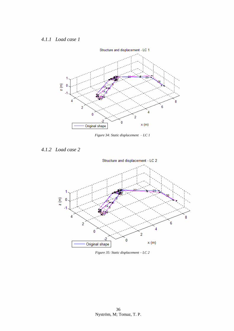
4.1.1 Load case 1
Figure 34: Static displacement – LC 1
4.1.2 Load case 2
Figure 35: Static displacement – LC 2

37
Nyström, M; Tomaz, T. P.
4.1.3 Load case 3
Figure 36: Static displacement – LC 3
4.1.4 Load case 4
Figure 37: Static displacement – LC 4

38
Nyström, M; Tomaz, T. P.
4.1.5 Load case 5
Figure 38: Static displacement – LC 5
4.1.6 Load case 6
Figure 39: Static displacement – LC 6

39
Nyström, M; Tomaz, T. P.
4.1.7 Load case 7
Figure 40: Static displacement – LC 7
4.2 Dynamic analysis
The results for the dynamic analyses are shown in this section. The dynamic
response for DOFs 73, 74 and 75 (displacement in the x, y and z-axis
directions) in the crane tip are shown. Also, the energy response, excluding
the time interval 0 < t < 0.08 [s], is shown for each load case.
This time interval is excluded from the energy calculations since these initial
timesteps contain a lot of disturbance information stemming from high
frequencies due to high axial stiffness compared to low mass for short
elements in the model.
The displacements for the timestep when the potential energy is at its
maximum is shown in Table 7. Complete displacement results can be found
in Appendix 9.
The forces and moments at node ends for the first boom are shown in Table
8 together with information about the maximum energy for each load case
and the time when the maximum occurs.

40
Nyström, M; Tomaz, T. P.
Table 7: Displacement for timestep with maximum energy – First boom
Node DOF LC1 LC2 LC3 LC4 LC5 LC6 LC7 Unit
2
7 8,6E-05 -7,6E-05 4,0E-05 0,0E+00 8,5E-05 6,5E-05 3,9E-05 [m]
8 -1,2E-04 1,1E-04 -5,1E-05 0,0E+00 -1,2E-04 -9,7E-05 -5,0E-05 [m]
9 0,0E+00 0,0E+00 0,0E+00 9,9E-04 7,5E-04 -1,6E-03 6,6E-04 [m]
10 0,0E+00 0,0E+00 0,0E+00 7,8E-03 5,7E-03 -1,3E-02 5,0E-03 [rad]
11 0,0E+00 0,0E+00 0,0E+00 -1,2E-03 -1,3E-03 1,1E-03 -1,3E-03 [rad]
143 -2,8E-03 1,8E-03 -2,2E-03 0,0E+00 -2,8E-03 -1,7E-03 -2,2E-03 [rad]
6
31 3,5E-03 -2,2E-03 3,0E-03 0,0E+00 3,5E-03 2,0E-03 3,0E-03 [m]
32 -4,5E-03 2,9E-03 -3,7E-03 0,0E+00 -4,4E-03 -2,7E-03 -3,6E-03 [m]
33 0,0E+00 0,0E+00 0,0E+00 1,4E-02 1,1E-02 -2,1E-02 1,0E-02 [m]
34 0,0E+00 0,0E+00 0,0E+00 7,8E-03 5,5E-03 -1,3E-02 4,8E-03 [rad]
35 0,0E+00 0,0E+00 0,0E+00 -2,5E-03 -2,7E-03 2,0E-03 -2,7E-03 [rad]
36 -2,6E-03 1,5E-03 -2,4E-03 0,0E+00 -2,6E-03 -1,4E-03 -2,4E-03 [rad]
7
37 6,0E-03 -2,8E-03 6,4E-03 0,0E+00 5,9E-03 2,8E-03 6,4E-03 [m]
38 -9,6E-03 4,8E-03 -9,7E-03 0,0E+00 -9,4E-03 -4,7E-03 -9,6E-03 [m]
39 0,0E+00 0,0E+00 0,0E+00 2,6E-02 2,2E-02 -3,7E-02 2,0E-02 [m]
40 0,0E+00 0,0E+00 0,0E+00 7,5E-03 5,1E-03 -1,3E-02 4,3E-03 [rad]
41 0,0E+00 0,0E+00 0,0E+00 -3,4E-03 -3,7E-03 2,5E-03 -3,8E-03 [rad]
42 -2,6E-03 3,9E-04 -4,0E-03 0,0E+00 -2,5E-03 -6,1E-04 -4,0E-03 [rad]
8
43 6,2E-03 -2,8E-03 6,7E-03 0,0E+00 6,1E-03 2,8E-03 6,6E-03 [m]
44 -1,0E-02 4,9E-03 -1,1E-02 0,0E+00 -1,0E-02 -4,9E-03 -1,1E-02 [m]
45 0,0E+00 0,0E+00 0,0E+00 2,8E-02 2,3E-02 -3,9E-02 2,1E-02 [m]
46 0,0E+00 0,0E+00 0,0E+00 7,5E-03 5,0E-03 -1,3E-02 4,2E-03 [rad]
47 0,0E+00 0,0E+00 0,0E+00 -3,5E-03 -3,8E-03 2,6E-03 -3,9E-03 [rad]
48 -2,6E-03 3,1E-04 -4,1E-03 0,0E+00 -2,5E-03 -5,4E-04 -4,0E-03 [rad]

41
Nyström, M; Tomaz, T. P.
Table 8: DOF forces and moments for timestep with maximum energy - First boom
Element Node
Element
Coor-
dinate
LC1 LC2 LC3 LC4 LC5 LC6 LC7 Unit
8 2
x -140,3 127,3 -56,0 0,0 -139,6 -112,0 -54,8 [kN]
y -3,0 8,1 6,6 0,0 -3,2 -6,2 6,7 [kN]
z 0,0 0,0 0,0 10,7 9,9 -12,5 9,5 [kN]
mx 0,0 0,0 0,0 -15,3 -20,0 3,9 -21,2 [kNm]
my 0,0 0,0 0,0 -52,3 -52,1 51,7 -51,4 [kNm]
mz 0,0 0,0 0,0 0,0 0,0 0,0 0,0 [kNm]
11 6
x 13,6 0,0 23,4 0,0 13,1 2,0 23,3 [kN]
y 70,3 -2,9 120,0 0,0 67,9 10,5 119,4 [kN]
z 0,0 0,0 0,0 0,0 0,0 -0,6 0,0 [kN]
mx 0,0 0,0 0,0 0,0 0,0 0,0 0,0 [kNm]
my 0,0 0,0 0,0 0,0 0,0 0,0 0,0 [kNm]
mz 0,0 0,0 0,0 0,0 0,0 0,0 0,0 [kNm]
12 7
x -67,8 114,1 51,3 0,0 -69,3 -92,9 51,9 [kN]
y 22,9 -38,7 -17,4 0,0 23,4 31,5 -17,6 [kN]
z 0,0 0,0 0,0 0,0 0,0 0,0 0,0 [kN]
mx 0,0 0,0 0,0 0,0 0,0 0,0 0,0 [kNm]
my 0,0 0,0 0,0 0,0 0,0 0,0 0,0 [kNm]
mz 0,0 0,0 0,0 0,0 0,0 0,0 0,0 [kNm]
10 8
x -46,8 85,9 46,5 0,0 -48,1 -69,7 46,9 [kN]
y 54,6 -106,8 -63,5 0,0 56,3 85,8 -63,9 [kN]
z 0,0 0,0 0,0 8,2 8,4 -7,7 8,3 [kN]
mx 0,0 0,0 0,0 -15,4 -20,0 4,1 -21,3 [kNm]
my 0,0 0,0 0,0 -9,8 -11,7 5,0 -12,2 [kNm]
mz 0,0 0,0 0,0 0,0 0,0 0,0 0,0 [kNm]
Time_max 0,2556 0,3486 0,2497 0,2789 0,2591 0,5309 0,2527 [s]
Energy_max 927,71 649,68 1004,5 288,19 1186,8 789,82 1245 [Nm²]

42
Nyström, M; Tomaz, T. P.
4.2.1 Load case 1
Figure 41: Dynamic response for the crane tip – LC 1
Figure 42: Energy response in the main boom - LC 1

43
Nyström, M; Tomaz, T. P.
4.2.2 Load case 2
Figure 43: Dynamic response for the crane tip – LC 2
Figure 44: Energy response in the main boom - LC 2

44
Nyström, M; Tomaz, T. P.
4.2.3 Load case 3
Figure 45: Dynamic response for the crane tip – LC 3
Figure 46: Energy response in the main boom - LC 3

45
Nyström, M; Tomaz, T. P.
4.2.4 Load case 4
Figure 47: Dynamic response for the crane tip – LC 4
Figure 48: Energy response in the main boom - LC 4

46
Nyström, M; Tomaz, T. P.
4.2.5 Load case 5
Figure 49: Dynamic response for the crane tip – LC 5
Figure 50: Energy response in the main boom - LC 5

47
Nyström, M; Tomaz, T. P.
4.2.6 Load case 6
Figure 51: Dynamic response for the crane tip – LC 6
Figure 52: Energy response in the main boom - LC 6

48
Nyström, M; Tomaz, T. P.
4.2.7 Load case 7
Figure 53: Dynamic response for the crane tip – LC 7
Figure 54: Energy response in the main boom - LC 7

49
Nyström, M; Tomaz, T. P.
4.3 Finite Element analysis
The results for the Finite Element analyses are shown in this section, both
for the first step (hot-spot method) and second step (notch stress method).
4.3.1 First step: hot-spot stresses
In this section, three results for each load case are shown. The first figure of
each load case corresponds to a general view from the highest principal
stresses using the tool isoclipping from the software. The second one is a
close up on the hot-spots. Finally, the Von Mises stresses are shown.
4.3.1.1 Load case 1
Figure 55: Principal stress – Values above 10 MPa – LC 1
X
Y
Z

50
Nyström, M; Tomaz, T. P.
Figure 56: Principal stress hot-spots – LC 1
Figure 57: Von Mises stress – LC 1
X
Y
Z
X
Y
Z

51
Nyström, M; Tomaz, T. P.
4.3.1.2 Load case 2
Figure 58: Principal stress – Values above 25 MPa – LC 2
Figure 59: Principal stress hot-spots – LC 2
X
Y
Z
X
Y
Z

52
Nyström, M; Tomaz, T. P.
Figure 60: Von Mises stress – LC 2
4.3.1.3 Load case 3
Figure 61: Principal stress – Values above 20 MPa – LC 3
X
Y
Z
X
Y
Z

53
Nyström, M; Tomaz, T. P.
Figure 62: Principal stress hot-spots – LC 3
Figure 63: Von Mises stress – LC 3
X
Y
Z
X
Y
Z

54
Nyström, M; Tomaz, T. P.
4.3.1.4 Load case 4
Figure 64: Principal stress – Values above 25 MPa – LC 4
Figure 65: Principal stress hot-spots – LC 4
X
Y
Z
X
Y
Z

55
Nyström, M; Tomaz, T. P.
Figure 66: Von Mises stress – LC 4
4.3.1.5 Load case 5
Figure 67: Principal stress – Values above 50 MPa – LC 5
X
Y
Z
X
Y
Z

56
Nyström, M; Tomaz, T. P.
Figure 68: Principal stress hot-spots – LC 5
Figure 69: Von Mises stress – LC 5
X
Y
Z
X
Y
Z

57
Nyström, M; Tomaz, T. P.
4.3.1.6 Load case 6
Figure 70: Principal stress – Values above 25 MPa – LC 6
Figure 71: Principal stress hot-spots – LC 6
X
Y
Z
X
Y
Z

58
Nyström, M; Tomaz, T. P.
Figure 72: Von Mises stress – LC 6
4.3.1.7 Load case 7
Figure 73: Principal stress – Values above 50 MPa – LC 7
X
Y
Z
X
Y
Z

59
Nyström, M; Tomaz, T. P.
Figure 74: Principal stress hot-spots – LC 7
Figure 75: Von Mises stress – LC 7
X
Y
Z
X
Y
Z

60
Nyström, M; Tomaz, T. P.
4.3.2 Second step: notch stress method
The results from the Notch Stress Method analyses are presented in Figure
76 and Figure 77. The maximum principal stress obtained from the LC 5 is
shown, together with the stress distribution around the notch.
Figure 76: Stress distribution in the notch (1/2) – LC 5
Figure 77: Stress distribution in the notch (2/2) – LC 5
X
Y
Z
X
Y
Z
Maximum
principal stress
𝜎𝑚𝑎𝑥 = 165 𝑀𝑃𝑎
Analyzed
weld

61
Nyström, M; Tomaz, T. P.
4.4 Fatigue calculations
The results for the fatigue calculations are shown in this section. The stress
range 𝜎𝑟𝑎𝑛𝑔𝑒 is obtained based on the principal stresses from the notch stress
method. 𝑅 is the ratio of the minimum and maximum stresses. 𝑁 is the
number of cycles before failure for a weld class FAT-225 (𝑚 = 3) with a
probability of survival of 97,7% (Fricke, 2007) and 𝑁𝑓 is the number of
cycles for the analyzed weld.
𝜎𝑚𝑎𝑥 = 165 𝑀𝑃𝑎 ( 63 )
𝜎𝑚𝑖𝑛 = −165 𝑀𝑃𝑎 ( 64 )
𝜎𝑟𝑎𝑛𝑔𝑒 = 𝜎𝑚𝑎𝑥 − 𝜎𝑚𝑖𝑛 = 330 𝑀𝑃𝑎 ( 65 )
𝑅 =𝜎𝑚𝑖𝑛
𝜎𝑚𝑎𝑥= −1 ( 66 )
𝑁𝑓 = 𝑁 (𝜎𝐹𝐴𝑇
𝜎𝑟𝑎𝑛𝑔𝑒)𝑚
= 2 ∙ 106 (225
330)3
= 633921 𝑐𝑦𝑐𝑙𝑒𝑠 ( 67 )
4.5 Damping experiment
The displacement response from the crane’s experiment for the DOF 74 is
shown in Figure 78, together with the exponential decay curve and the
adjusted curve, in order to show how the experiment relates to the theory.
The adjusted curve is obtained by trial, using the experimental curve as
reference and correlating it with the theoretical proposal of the equation of
motion for a system in free vibration having viscous damping (Rajasekaran,
2009).
Figure 78: Damping experiment curve

62
Nyström, M; Tomaz, T. P.
The adjusted/approximation curve ua(t) and its derivative with respect to
time are,
𝑢𝑎(𝑡) = −𝑒−0,45𝑡 ∙ 0,055𝑠𝑖𝑛(8,3𝑡 + 1,6) + 0,0022𝑡 − 0,014⏟
𝑂𝑓𝑓𝑠𝑒𝑡 𝑎𝑑𝑗𝑢𝑠𝑡𝑚𝑒𝑛𝑡
( 68 )
𝑑
𝑑𝑡(𝑢𝑎(𝑡)) = (0,02475𝑒
−0,45𝑡 ∙ 𝑠𝑖𝑛(8,3𝑡 + 1,6)
− 0,4565𝑒−0,45𝑡 ∙ 𝑐𝑜𝑠(8,3𝑡 + 1,6) + 0,0022)
( 69 )
Evaluating the derivative for each timestep it is possible to determine when
the slope changes, and then, the period 𝑇𝑛 is obtained,
𝑇𝑛 = 0.38 [𝑠] ( 70 )
The natural circular frequency ωn can be written as
𝜔𝑛 =
2𝜋
𝑇𝑛= 16.53 [𝑟𝑎𝑑/𝑠]
( 71 )
Comparing the adjusted curve 𝑢𝑎(𝑡) with the formula suggested by the book
“Structural Dynamics for Earthquake Engineering” (Rajasekaran, 2009), it
is possible to show that the damping coefficient ξ is
𝑢(𝑡) = 𝑒−𝜉∙𝜔𝑛∙𝑡 ∙ (𝐴 ∙ 𝑠𝑖𝑛 (𝜔𝑛 ∙ √1 − 𝜉2𝑡 + 𝜑)) ( 72 )
𝜉 ∙ 𝜔𝑛 = 0.45 ( 73 )
𝜉 =
0,45
𝜔𝑛= 0.027 = 2.7%
( 74 )

63
Nyström, M; Tomaz, T. P.
5. Analysis
The load case resulting in the highest energy was the LC 7, as expected,
when all the actuators are fully loaded. It is possible to observe a correlation
between potential energy and hot-spot stresses, as shown in Table 9.
Table 9: Potential energy and Hot-spot stress correlation
Variable LC1 LC2 LC3 LC4 LC5 LC6 LC7 Unit
Hotspot_stress 50 40 20 40 65 45 70 [MPa]
Energy_max 927,71 649,68 1004,5 288,19 1186,8 789,82 1245 [Nm²]
Figure 79: Potential energy x stress correlation
From the hot-spot method analysis, it is possible to observe that there are
common hot-spots for more than one load case. This behavior can be seen in
Figure 80, Figure 81 and Figure 82. In Figure 80, LC 5 corresponds to the
hot-spot analyzed in previous sections. This is an indication that these spots
are candidates for possible weld failures.

64
Nyström, M; Tomaz, T. P.
Figure 80: Common hot-spot stresses – Case 1
Figure 81: Common hot-spot stresses- Case 2
Figure 82: Common hot-spot stresses- Case 3

65
Nyström, M; Tomaz, T. P.
6. Discussion
It is possible to conclude, from the presented results and from the analyses,
that both the Euler-Bernoulli beam FE model and the a 3D solid
CAD-model behaves in a compatible way with the real life crane from some
perspectives, such as the deformed shape and stress levels. This is indicating
that the calculations done for the fatigue life length are valid.
Our suggestions for future studies are:
Adjust the damping coefficient in the model according to
experimental data
Use of the damage summation theory (Palmgren-Miner) to quantify
different loadings from the load cases
Perform the analyses for other hot-spots and other crane components
Study the relation between the varying stress direction in the notch
and the fatigue life
Eliminate the axial stiffness from the beam element, in order to
remove the high eigenfrequencies associated with axial vibrations.

66
Nyström, M; Tomaz, T. P.
7. Conclusions
The results from the thesis were obtained according to the standards and the
recent literature about the subject. The aim and purpose of the work were
contemplated.
Progress on the research of the assessment methods for fatigue calculations
is concluded but there is more to be done in further studies.
The methods used in this thesis fulfilled the company's requirements and the
results are expected to contribute in further product development, since the
crane model works fine and the results revealed important crane properties.
Also, the method is general and can be applied to the design procedure for
the company’s wide product range.

67
Nyström, M; Tomaz, T. P.
References
Akhlaghi, F. Z., 2009. Fatigue life assessment of welded bridge details using
structural hot spot stress method, Göteborg, Sweden: s.n.
Assan, A. E., 2013. Método dos Elementos Finitos (Finite Element Method). 2nd
ed. Campinas: Editora da Unicamp. Language: Portuguese.
Austrell, P. E. et al., 2004. CALFEM - A finite element toolbox. 3.4 ed. Lund,
Sweden: Lund University.
Craig, R. R. & Kurdila, A. J., 2011. Fundamentals of Structural Dynamics. 2nd
ed. s.l.:John Wiley & Sons.
Ekevid, T., 2014. Course: The Finite Element Method, Växjö: s.n.
Eriksson, Å., Lignell, A.-M., Olsson, C. & Spennare, H., 2002. Svetsutvärdering
med FEM. Stockholm: Industrilitteratur AB.
European prestandard, 2002. EN 1993-1.9:2002.E - Eurocode 3: Design of steel
structures. Part 1.9: Fatigue strength of steel structures, Brussels: Eurocode.
FAO, 2010. Global Forest Resources Assessment, Rome: Food and Agriculture
Organization of the United Nations.
Fricke, W., 2007. Round-robin study on stress analysis for the effective notch
stress approach. Welding in the world, 51(3/4), pp. 68-79.
Fricke, W., 2008. Guideline for the Fatigue Assessment by Notch Stress Analysis
for Welded Structures, s.l.: International Institute of Welding (IIW).
Haibach, E., 1968. Die Schwingfestigkeit von Schweißverbindungen aus der
Sicht einer örtlichen Beanspruchungsmessung (The fatigue strength of welded
joints considered on the basis of a local stress measurement), Darmstadt,
Germany: Fraunhofer-Inst. für Betriebsfestigkeit. Language: German.
Hobbacher, A., 2008. Recommendations for Fatigue Design of Welded Joints
and Components, Paris, France: IIW.
Hyun Kim, M. et al., 2009. A comparative study for the fatigue assessment of a
ship structure by use of hot spot stress and structural stress approaches. Ocean
Engineering, Issue 36, pp. 1067-1072.
Johansson, M., 2011. Structural properties of sawn timber and engineered wood
products. In: P. Bergkvist, ed. Design of timber structures. 1st ed. Stockholm:
Swedish Forest Industries Federation.
Linköping universitetet, 1995. Hydraulvätska. In: Formelsamling i hydraulik och
pneumatik. Linköping, Sweden: Linköping universitetet.
Lussanet, M. H. E. d., Smeets, J. B. J. & Brenner, E., 2002. Relative damping
improves linear mass-spring models of goal-directed movements. Human
Movement Science, pp. 85-100.
Macdonald, K., 2011. Fracture and Fatigue of Welded Joints and Structures.
Second ed. Cambridge: Elsevier.
Marin, T. & Nicoletto, G., 2009. Fatigue design of welded joints using the finite
element method and the 2007 ASME Div.2 Master Curve. Frattura ed Integrità
Strutturale, Volume 9, pp. 76-84.
Ottosen, N. & Petersson, H., 1992. Introduction to the Finite Element Method.
s.l.:Prentice Hall.
Pedersen, M., Mouritsen, O., Hansen, M. & Andersen, J., 2010. Experience with
the Notch Stress Approach for Fatigue Assessment of Welded Joints. Borlänge,

68
Nyström, M; Tomaz, T. P.
Sweden, Proceedings of Swedish Conference on Lightweight Optimised Welded
Structures, LOST. Kungliga Tekniska Högskolan.
Radaj, D., Sonsino, C. & Fricke, W., 2009. Recent developments in local
concepts of fafigue of welded joints. International Journal of Fatigue, Volume
31, pp. 2-11.
Rajasekaran, S., 2009. Free vibration of single-degree-of-freedom systems
(under-damped) in relation to structural dynamics during earthquakes. In:
Structural dynamics of earthquake engineering. 1st ed. Boca Raton: Woodhead
Publishing Limited, pp. 43-67.
Rao, S., 2004. The finite element method in engineering. 4th ed. Miami: Elsevier
Science & Technology Books.
Ritchie, R., 1998. Mechanisms of fatigue-crack propagation in ductile and brittle
solids. International Journal of Fatigue, Volume 100, pp. 55-83.
Rother, K. & Rudolph, J., 2010. Fatigue assessment of welded structures:
practical aspects for stress analysis and fatigue assessment. Fatigue & Fracture
of Engineering Material & Structures, Volume 34, pp. 177-204.
Rottne Industri AB, 2014. Rottne - First in forest. [Online]
Available at: http://www.rottne.com/
[Accessed 20 02 2015].
Sonsino, C. et al., 2012. Notch stress concepts for the fatigue assessment of
welded joints - Background and applications. International Journal of Fatigue,
Volume 34, pp. 2-16.
Swedish Forest Industries, T., 2013. Forest industry - Facts and figures. [Online]
Available at:
http://www.forestindustries.se/documentation/publications_and_surveys
[Accessed 20 02 2014].
Timoshenko, S., 1983. History of strength of materials. 1st ed. New York: Dover
Publications.
Witek, L., 2009. Experimental crack propagation and failure analysis of the first
stage compressor blade subjected to vibration. Engineering Failure Analysis,
Volume 16, pp. 2163-2170.

69
Nyström, M; Tomaz, T. P.
Appendices
Appendix 1: Beam type element according to CALFEM
Appendix 2: Palmgren-Miner example
Appendix 3: Mass and stiffness matrices
Appendix 4: Model element coordinates
Appendix 5: Model element node-number and connections
Appendix 6: Model element degree-of-freedom
Appendix 7: Model element properties
Appendix 8: Static displacement
Appendix 9: Displacement for dynamic analysis
Appendix 10: MATLAB codes

Appendix 1: page 1/1
Nyström, M; Tomaz, T. P.
APPENDIX 1: Beam type element according to CALFEM
The beam type element used by the CALFEM toolbox is based on the Euler-
Bernoulli beam. A basic representation with signal rule is presented in Figure 83 and
Figure 84.
Figure 83: Beam element orientation (Austrell, et al., 2004)
Figure 84: Beam element section forces orientation (Austrell, et al., 2004)

Appendix 2: page 1/1
Nyström, M; Tomaz, T. P.
APPENDIX 2: Palmgren-Miner example
A short example of Palmgren-Miner is given: assume that Figure 3 represents a
material’s structure and that this structure has the following loading cycles: 10
loadings of stress type 1, 500 loadings of type 2, 103 loadings of type 3 and 1500
loadings for type 4. Suppose maximum number of cycles for each type is N1 =102; 𝑁2 = 10
3; N3 = 5000; N4 = 104.
∑
𝑛𝑖𝑁𝑖
𝐼
𝑖=1
=10
102+500
103+103
5000+1500
104= 0,95
( 75 )
Since:
∑𝑛𝑖𝑁𝑖
𝐼
𝑖=1
< 1
( 76 )
The structure has enough strength to withstand to fatigue.

Appendix 3: page 1/2
Nyström, M; Tomaz, T. P.
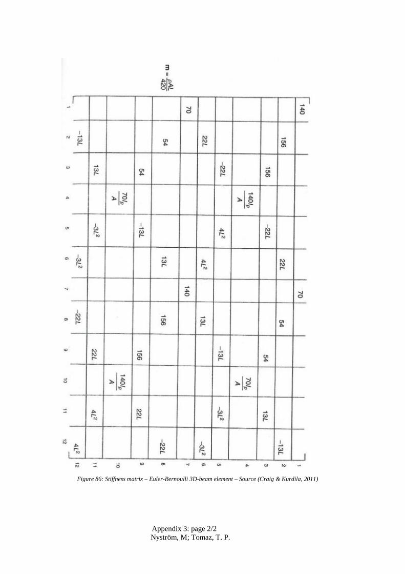
APPENDIX 3: Mass and stiffness matrices
The mass and stiffness matrices for an Euler-Bernoulli 3D-beam element can be seen
in Figure 85 and Figure 86, where 𝐴 is the element’s cross-sectional area, 𝐼𝑦 and 𝐼𝑧
are the area moments of inertia of the cross section, 𝐼𝑝 is the area polar moment of
inertia about the “x” axis, 𝐿 is the element’s length, 𝐸 is the modulus of elasticity, 𝐺𝐽 is the torsional stiffness and ρ is the mass density
.
Figure 85: Mass matrix – Euler-Bernoulli 3D-beam element – Source (Craig & Kurdila, 2011)
Appendix 3: page 2/2
Nyström, M; Tomaz, T. P.
Figure 86: Stiffness matrix – Euler-Bernoulli 3D-beam element – Source (Craig & Kurdila, 2011)

Appendix 4: page 1/1
Nyström, M; Tomaz, T. P.
APPENDIX 4: Model element coordinates
The crane coordinates and element length is shown in Table 10.
Table 10: Element coordinates table
Element
number
X start
(mm)
X end
(mm)
Y start
(mm)
Y end
(mm)
Z start
(mm)
Z end
(mm)
Length
(mm)
1 0 696 698 698 0 0 696,0
2 696 696 698 923 0 0 225,0
3 62,19 100,41 1377,73 1350,31 0 0 47,0
4 100,41 251,49 1350,31 1241,92 0 0 185,9
5 251,49 696 1241,92 923 0 0 547,1
6 100,41 420,71 1350,31 1796,74 0 0 549,4
7 251,49 477,11 1241,92 1556,4 0 0 387,0
8 696 2395 923 1973,42 0 0 1997,5
9 2395 4130,58 1973,42 3046,46 0 0 2040,5
1 4130,58 4353,43 3046,46 3184,24 0 0 262,0
11 2395 2244,6 1973,42 2216,69 0 0 286,0
12 4130,58 4085,88 3046,46 3118,76 0 0 85,0
13 420,71 3651,35 1796,74 3600,32 0 0 3700,0
14 477,11 2244,6 1556,4 2216,69 0 0 1886,8
15 3651,35 3953,86 3600,32 3583,25 0 0 303,0
16 3953,86 4365,69 3583,25 3560,67 0 0 412,4
17 3953,86 3958,71 3583,25 3669,26 0 0 86,1
18 4085,88 3958,71 3118,76 3669,26 0 0 565,0
19 4365,69 4550,21 3560,67 3796,84 0 0 299,7
20 4353,43 4734,84 3184,24 3643,51 0 0 597,0
21 4550,21 4734,84 3796,84 3643,51 0 0 240,0
22 4734,84 6896,59 3643,51 1848,26 0 0 2810,0
23 6896,59 7909,24 1848,26 1007,29 0 0 1316,3
24 -25 62,19 698 1377,73 0 0 685,3
25 -25 0 698 698 0 0 25,0
26 7909,24 7909,24 1007,29 -1492,71 0 0 2500,0

Appendix 5: page 1/1
Nyström, M; Tomaz, T. P.
APPENDIX 5: Model element node-number and
connections
Some elements are connected by pin or ball joint. Pin joints are free to move in one
rotational DOF around “y” axis. Ball joints are free to move around the three
rotational axis. Pin joints are represented by number 1 and ball joints by number 3, as
seen in Table 11.
Table 11: Element node and connections type
Element
number
Node
start
Connection
start
Node
end
Connection
end
1 22 14
2 14 2 1
3 3 3 15
4 15 16
5 16 2 1
6 15 4 3
7 16 5 3
8 2 1 17
9 17 18
1 18 8 1
11 17 6 3
12 18 7 3
13 4 3 9 3
14 5 3 6 3
15 9 3 19
16 19 11 1
17 19 10 3
18 7 3 10 3
19 11 1 20
20 8 1 21
21 20 21
22 21 12
23 12 13 3
24 1 3 3 3
25 1 3 22
26 13 3 23
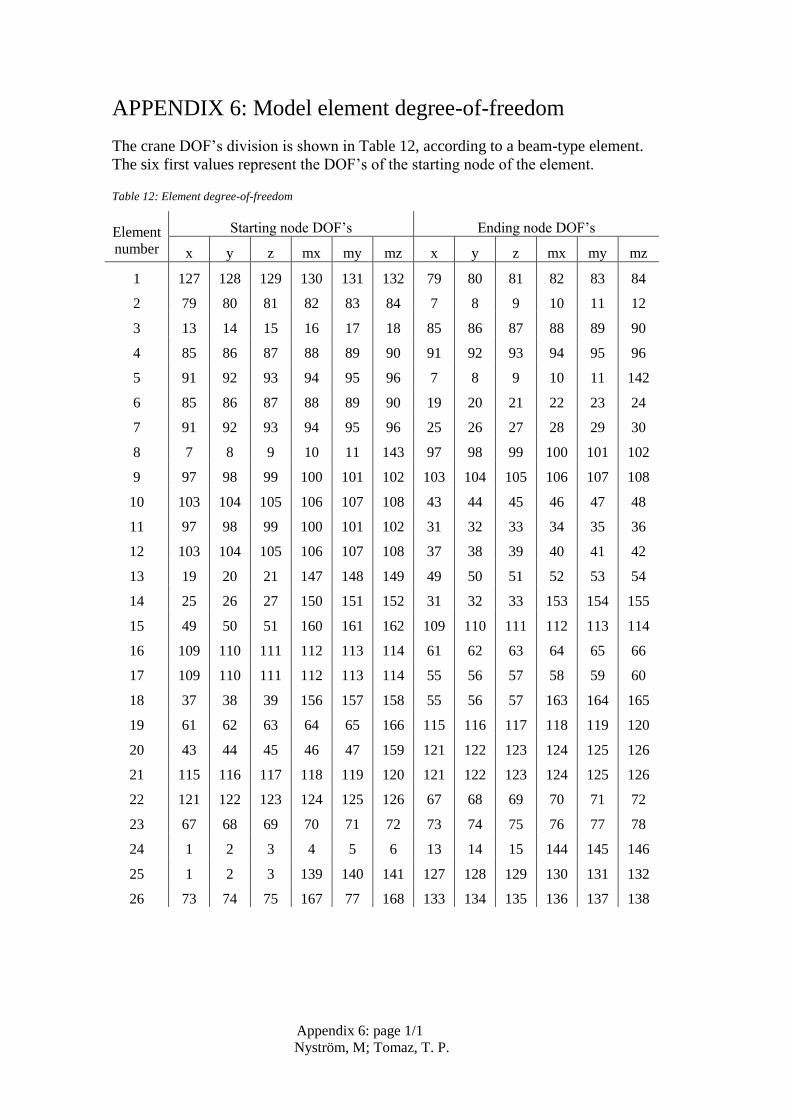
Appendix 6: page 1/1
Nyström, M; Tomaz, T. P.
APPENDIX 6: Model element degree-of-freedom
The crane DOF’s division is shown in Table 12, according to a beam-type element.
The six first values represent the DOF’s of the starting node of the element.
Table 12: Element degree-of-freedom
Element
number
Starting node DOF’s Ending node DOF’s
x y z mx my mz x y z mx my mz
1 127 128 129 130 131 132 79 80 81 82 83 84
2 79 80 81 82 83 84 7 8 9 10 11 12
3 13 14 15 16 17 18 85 86 87 88 89 90
4 85 86 87 88 89 90 91 92 93 94 95 96
5 91 92 93 94 95 96 7 8 9 10 11 142
6 85 86 87 88 89 90 19 20 21 22 23 24
7 91 92 93 94 95 96 25 26 27 28 29 30
8 7 8 9 10 11 143 97 98 99 100 101 102
9 97 98 99 100 101 102 103 104 105 106 107 108
10 103 104 105 106 107 108 43 44 45 46 47 48
11 97 98 99 100 101 102 31 32 33 34 35 36
12 103 104 105 106 107 108 37 38 39 40 41 42
13 19 20 21 147 148 149 49 50 51 52 53 54
14 25 26 27 150 151 152 31 32 33 153 154 155
15 49 50 51 160 161 162 109 110 111 112 113 114
16 109 110 111 112 113 114 61 62 63 64 65 66
17 109 110 111 112 113 114 55 56 57 58 59 60
18 37 38 39 156 157 158 55 56 57 163 164 165
19 61 62 63 64 65 166 115 116 117 118 119 120
20 43 44 45 46 47 159 121 122 123 124 125 126
21 115 116 117 118 119 120 121 122 123 124 125 126
22 121 122 123 124 125 126 67 68 69 70 71 72
23 67 68 69 70 71 72 73 74 75 76 77 78
24 1 2 3 4 5 6 13 14 15 144 145 146
25 1 2 3 139 140 141 127 128 129 130 131 132
26 73 74 75 167 77 168 133 134 135 136 137 138

Appendix 7: page 1/2
Nyström, M; Tomaz, T. P.
APPENDIX 7: Model element properties
The element properties were taken from the FEM-model. Cross-sectional area (A),
area moment of inertia (Iy, Iz) and torsional constant (Kv) were taken based on the
main cross-section of the element. Polar mass moment of inertia (J) and mass per
unit length (m) were taken from the complete FEM-model. Shear modulus of
elasticity G = 79000 MPa and modulus of elasticity E = 210000 MPa for alloy
steel. Actuators (elements 14 and 24) have a specific modulus of elasticity (E14 =49950 MPa and E24 = 24920 MPa).
Table 13: Element properties
Element
number E G
A
[m2]
Iy
[m4]
Iz
[m4]
Kv
[m4]
m
[kg/m]
J
[kg/m2]
1 E G 5,0E-02 4,6E-04 1,6E-04 6,1E-04 2,7E+02 3,3E+00
2 E G 3,0E-02 2,3E-06 1,6E-04 1,6E-04 2,3E+02 2,7E-01
3 E G 1,7E-02 5,7E-07 2,7E-04 2,7E-04 2,1E+02 6,6E-02
4 E G 1,7E-02 5,7E-07 2,7E-04 2,7E-04 2,1E+02 2,6E-01
5 E G 1,1E-02 3,6E-07 6,8E-05 6,9E-05 1,1E+02 3,4E-01
6 E G 1,7E-02 5,7E-07 2,7E-04 2,7E-04 1,0E+00 1,0E-03
7 E G 1,7E-02 5,7E-07 2,7E-04 2,7E-04 1,0E+00 1,0E-03
8 E G 1,3E-02 3,5E-04 2,1E-04 5,6E-04 2,1E+02 3,4E+00
9 E G 1,3E-02 3,5E-04 2,1E-04 5,6E-04 2,1E+02 2,0E+00
10 E G 1,3E-02 3,5E-04 2,1E-04 5,6E-04 1,8E+02 2,9E-01
11 E G 1,3E-02 3,5E-04 2,1E-04 5,6E-04 1,0E+00 1,0E-03
12 E G 1,3E-02 3,5E-04 2,1E-04 5,6E-04 1,0E+00 1,0E-03
13 E G 2,5E-03 4,9E-06 3,7E-06 8,6E-06 3,2E+01 5,3E-01
14 E14 G 3,8E-03 1,2E-06 1,2E-06 2,4E-06 1,1E+02 1,1E+00
15 E G 1,0E-02 5,2E-07 3,3E-05 3,4E-05 1,2E+02 1,6E-01
16 E G 1,0E-02 5,2E-07 3,3E-05 3,4E-05 1,1E+02 1,1E-01
17 E G 1,0E-02 5,2E-07 3,3E-05 3,4E-05 1,0E+00 1,1E-01
18 E G 5,0E-03 2,6E-07 4,2E-06 4,4E-06 3,9E+01 3,0E-02
19 E G 5,8E-03 5,0E-05 6,5E-05 1,1E-04 1,0E+00 2,7E-01
20 E G 5,8E-03 5,0E-05 6,5E-05 1,1E-04 1,0E+00 5,4E-01
21 E G 9,1E-03 9,1E-05 3,5E-04 4,4E-04 4,1E+02 9,0E-01
22 E G 5,8E-03 5,0E-05 6,5E-05 1,1E-04 1,7E+02 3,4E+00
23 E G 4,9E-03 3,0E-05 4,0E-05 7,0E-05 1,1E+02 4,6E-01
24 E24 G 5,0E-03 2,0E-06 2,0E-06 4,0E-06 2,6E+02 1,2E+00
25 E G 1,5E-02 1,1E-06 7,8E-05 7,9E-05 1,2E+02 1,4E-01
26 E G 8,3E-02 5,7E-04 5,7E-04 1,1E-03 6,4E+02 2,3E+01

Appendix 7: page 2/2
Nyström, M; Tomaz, T. P.
A specific calculation was done in order to obtain the modulus of elasticity for the
actuators, based on “Formelsamling i Hydraulik och pneumatic” (Linköping
universitetet, 1995), where β is the average value for the compressibility of the
hydraulic oil (bulk modulus of elasticity). L14, L24 are the element lengths in the
model and Lc14, Lc24 are the oil lengths in the actuators.
𝛽 = 1,6𝑒10 ( 77 )
𝐿14 = 1,767 𝑚 ( 78 )
𝐿24 = 0,6853 𝑚 ( 79 )
𝐿𝑐14 = 0,566 𝑚 ( 80 )
𝐿𝑐24 = 0,44 𝑚 ( 81 )
The modulus of elasticity for each actuator is shown below.
𝐸14 =
𝛽 ∙ 𝐿14
𝐿𝑐14= 49950 𝑀𝑃𝑎
( 82 )
𝐸24 =
𝛽 ∙ 𝐿24
𝐿𝑐24= 24920 𝑀𝑃𝑎
( 83 )

Appendix 8: page 1/4
Nyström, M; Tomaz, T. P.
APPENDIX 8: Static displacement
The complete results for static displacement is shown in Table 14.
Table 14: Static displacement
DOF LC1 LC2 LC3 LC4 LC5 LC6 LC7
1 -3,6E-12 1,8E-07 1,8E-07 0,0E+00 -3,6E-12 1,8E-07 1,8E-07
2 -1,1E-12 5,6E-08 5,6E-08 0,0E+00 -1,1E-12 5,6E-08 5,6E-08
3 0,0E+00 0,0E+00 0,0E+00 1,1E-20 1,1E-20 1,1E-20 1,1E-20
4 0,0E+00 0,0E+00 0,0E+00 7,4E-02 7,4E-02 7,4E-02 7,4E-02
5 0,0E+00 0,0E+00 0,0E+00 5,8E-01 5,8E-01 5,8E-01 5,8E-01
6 -6,0E-05 -1,8E-03 -1,9E-03 0,0E+00 -6,0E-05 -1,9E-03 -1,8E-03
7 2,0E-05 2,9E-04 3,1E-04 0,0E+00 2,0E-05 3,1E-04 2,9E-04
8 -2,6E-05 -6,3E-04 -6,5E-04 0,0E+00 -2,6E-05 -6,5E-04 -6,3E-04
9 0,0E+00 0,0E+00 0,0E+00 -2,7E-04 -2,7E-04 -2,7E-04 -2,7E-04
10 0,0E+00 0,0E+00 0,0E+00 -8,1E-04 -8,1E-04 -8,1E-04 -8,1E-04
11 0,0E+00 0,0E+00 0,0E+00 1,5E-03 1,5E-03 1,5E-03 1,5E-03
12 -8,9E-05 -1,3E-03 -1,4E-03 0,0E+00 -8,9E-05 -1,4E-03 -1,3E-03
13 4,1E-05 1,4E-03 1,4E-03 0,0E+00 4,1E-05 1,4E-03 1,4E-03
14 -5,3E-06 8,0E-04 8,0E-04 0,0E+00 -5,3E-06 8,0E-04 8,0E-04
15 0,0E+00 0,0E+00 0,0E+00 3,2E-04 3,2E-04 3,2E-04 3,2E-04
16 0,0E+00 0,0E+00 0,0E+00 -8,1E-04 -8,1E-04 -8,1E-04 -8,1E-04
17 0,0E+00 0,0E+00 0,0E+00 1,5E-03 1,5E-03 1,5E-03 1,5E-03
18 1,2E-04 -2,5E-03 -2,4E-03 0,0E+00 1,2E-04 -2,4E-03 -2,5E-03
19 -4,7E-05 2,5E-03 2,4E-03 0,0E+00 -4,7E-05 2,4E-03 2,5E-03
20 5,0E-05 -1,2E-04 -6,6E-05 0,0E+00 5,0E-05 -6,6E-05 -1,2E-04
21 0,0E+00 0,0E+00 0,0E+00 -5,6E-04 -5,6E-04 -5,6E-04 -5,6E-04
22 0,0E+00 0,0E+00 0,0E+00 -8,1E-04 -8,1E-04 -8,1E-04 -8,1E-04
23 0,0E+00 0,0E+00 0,0E+00 1,5E-03 1,5E-03 1,5E-03 1,5E-03
24 2,2E-04 -2,7E-03 -2,4E-03 0,0E+00 2,2E-04 -2,4E-03 -2,7E-03
25 6,9E-05 1,8E-03 1,9E-03 0,0E+00 6,9E-05 1,9E-03 1,8E-03
26 1,3E-05 -2,1E-04 -2,0E-04 0,0E+00 1,3E-05 -2,0E-04 -2,1E-04
27 0,0E+00 0,0E+00 0,0E+00 -4,5E-04 -4,5E-04 -4,5E-04 -4,5E-04
28 0,0E+00 0,0E+00 0,0E+00 -8,1E-04 -8,1E-04 -8,1E-04 -8,1E-04
29 0,0E+00 0,0E+00 0,0E+00 1,5E-03 1,5E-03 1,5E-03 1,5E-03
30 -5,4E-05 -2,4E-03 -2,5E-03 0,0E+00 -5,4E-05 -2,5E-03 -2,4E-03
31 2,3E-03 3,5E-03 5,7E-03 0,0E+00 2,3E-03 5,7E-03 3,5E-03
32 -2,6E-03 -4,7E-03 -7,3E-03 0,0E+00 -2,6E-03 -7,3E-03 -4,7E-03
33 0,0E+00 0,0E+00 0,0E+00 -4,5E-03 -4,5E-03 -4,5E-03 -4,5E-03
34 0,0E+00 0,0E+00 0,0E+00 -2,4E-04 -2,4E-04 -2,4E-04 -2,4E-04
35 0,0E+00 0,0E+00 0,0E+00 3,2E-03 3,2E-03 3,2E-03 3,2E-03
36 -1,9E-03 -2,3E-03 -4,2E-03 0,0E+00 -1,9E-03 -4,2E-03 -2,3E-03
37 5,4E-03 4,8E-03 1,0E-02 0,0E+00 5,4E-03 1,0E-02 4,8E-03
38 -7,9E-03 -8,1E-03 -1,6E-02 0,0E+00 -7,9E-03 -1,6E-02 -8,1E-03

Appendix 8: page 2/4
Nyström, M; Tomaz, T. P.
39 0,0E+00 0,0E+00 0,0E+00 -1,1E-02 -1,1E-02 -1,1E-02 -1,1E-02
40 0,0E+00 0,0E+00 0,0E+00 5,7E-04 5,7E-04 5,7E-04 5,7E-04
41 0,0E+00 0,0E+00 0,0E+00 4,6E-03 4,6E-03 4,6E-03 4,6E-03
42 -3,8E-03 -1,1E-03 -4,9E-03 0,0E+00 -3,8E-03 -4,9E-03 -1,1E-03
43 5,6E-03 4,8E-03 1,0E-02 0,0E+00 5,6E-03 1,0E-02 4,8E-03
44 -9,0E-03 -8,4E-03 -1,7E-02 0,0E+00 -9,0E-03 -1,7E-02 -8,4E-03
45 0,0E+00 0,0E+00 0,0E+00 -1,2E-02 -1,2E-02 -1,2E-02 -1,2E-02
46 0,0E+00 0,0E+00 0,0E+00 6,9E-04 6,9E-04 6,9E-04 6,9E-04
47 0,0E+00 0,0E+00 0,0E+00 4,7E-03 4,7E-03 4,7E-03 4,7E-03
48 -3,9E-03 -9,7E-04 -4,9E-03 0,0E+00 -3,9E-03 -4,9E-03 -9,7E-04
49 3,4E-03 7,7E-03 1,1E-02 0,0E+00 3,4E-03 1,1E-02 7,7E-03
50 -7,4E-03 -7,5E-03 -1,5E-02 0,0E+00 -7,4E-03 -1,5E-02 -7,5E-03
51 0,0E+00 0,0E+00 0,0E+00 -7,1E-03 -7,1E-03 -7,1E-03 -7,1E-03
52 0,0E+00 0,0E+00 0,0E+00 -2,1E-02 -2,1E-02 -2,1E-02 -2,1E-02
53 0,0E+00 0,0E+00 0,0E+00 -9,8E-03 -9,8E-03 -9,8E-03 -9,8E-03
54 -2,2E-03 -2,4E-03 -4,6E-03 0,0E+00 -2,2E-03 -4,6E-03 -2,4E-03
55 3,6E-03 7,7E-03 1,1E-02 0,0E+00 3,6E-03 1,1E-02 7,7E-03
56 -8,3E-03 -7,5E-03 -1,6E-02 0,0E+00 -8,3E-03 -1,6E-02 -7,5E-03
57 0,0E+00 0,0E+00 0,0E+00 -8,9E-03 -8,9E-03 -8,9E-03 -8,9E-03
58 0,0E+00 0,0E+00 0,0E+00 2,0E-03 2,0E-03 2,0E-03 2,0E-03
59 0,0E+00 0,0E+00 0,0E+00 6,5E-03 6,5E-03 6,5E-03 6,5E-03
60 -2,8E-03 -4,8E-04 -3,3E-03 0,0E+00 -2,8E-03 -3,3E-03 -4,8E-04
61 3,3E-03 7,7E-03 1,1E-02 0,0E+00 3,3E-03 1,1E-02 7,7E-03
62 -9,3E-03 -7,9E-03 -1,7E-02 0,0E+00 -9,3E-03 -1,7E-02 -7,9E-03
63 0,0E+00 0,0E+00 0,0E+00 -1,2E-02 -1,2E-02 -1,2E-02 -1,2E-02
64 0,0E+00 0,0E+00 0,0E+00 2,0E-03 2,0E-03 2,0E-03 2,0E-03
65 0,0E+00 0,0E+00 0,0E+00 6,5E-03 6,5E-03 6,5E-03 6,5E-03
66 -2,3E-03 -1,3E-03 -3,6E-03 0,0E+00 -2,3E-03 -3,6E-03 -1,3E-03
67 2,3E-02 -1,6E-02 7,0E-03 0,0E+00 2,3E-02 7,0E-03 -1,6E-02
68 1,8E-02 -4,1E-02 -2,3E-02 0,0E+00 1,8E-02 -2,3E-02 -4,1E-02
69 0,0E+00 0,0E+00 0,0E+00 -4,2E-02 -4,2E-02 -4,2E-02 -4,2E-02
70 0,0E+00 0,0E+00 0,0E+00 5,9E-03 5,9E-03 5,9E-03 5,9E-03
71 0,0E+00 0,0E+00 0,0E+00 1,1E-02 1,1E-02 1,1E-02 1,1E-02
72 1,4E-02 -1,6E-02 -2,7E-03 0,0E+00 1,4E-02 -2,7E-03 -1,6E-02
73 3,5E-02 -3,0E-02 4,7E-03 0,0E+00 3,5E-02 4,7E-03 -3,0E-02
74 3,2E-02 -5,8E-02 -2,6E-02 0,0E+00 3,2E-02 -2,6E-02 -5,8E-02
75 0,0E+00 0,0E+00 0,0E+00 -5,9E-02 -5,9E-02 -5,9E-02 -5,9E-02
76 0,0E+00 0,0E+00 0,0E+00 6,6E-03 6,6E-03 6,6E-03 6,6E-03
77 0,0E+00 0,0E+00 0,0E+00 1,2E-02 1,2E-02 1,2E-02 1,2E-02
78 1,5E-02 -1,8E-02 -2,9E-03 0,0E+00 1,5E-02 -2,9E-03 -1,8E-02
79 1,1E-06 -1,4E-06 -3,3E-07 0,0E+00 1,1E-06 -3,3E-07 -1,4E-06
80 -2,6E-05 -6,2E-04 -6,5E-04 0,0E+00 -2,6E-05 -6,5E-04 -6,2E-04
81 0,0E+00 0,0E+00 0,0E+00 -1,6E-04 -1,6E-04 -1,6E-04 -1,6E-04
82 0,0E+00 0,0E+00 0,0E+00 -3,6E-05 -3,6E-05 -3,6E-05 -3,6E-05
83 0,0E+00 0,0E+00 0,0E+00 4,5E-04 4,5E-04 4,5E-04 4,5E-04

Appendix 8: page 3/4
Nyström, M; Tomaz, T. P.
84 -7,6E-05 -1,3E-03 -1,4E-03 0,0E+00 -7,6E-05 -1,4E-03 -1,3E-03
85 4,4E-05 1,3E-03 1,3E-03 0,0E+00 4,4E-05 1,3E-03 1,3E-03
86 -5,5E-07 7,1E-04 7,1E-04 0,0E+00 -5,5E-07 7,1E-04 7,1E-04
87 0,0E+00 0,0E+00 0,0E+00 2,9E-04 2,9E-04 2,9E-04 2,9E-04
88 0,0E+00 0,0E+00 0,0E+00 -8,1E-04 -8,1E-04 -8,1E-04 -8,1E-04
89 0,0E+00 0,0E+00 0,0E+00 1,5E-03 1,5E-03 1,5E-03 1,5E-03
90 1,2E-04 -2,5E-03 -2,4E-03 0,0E+00 1,2E-04 -2,4E-03 -2,5E-03
91 5,5E-05 1,0E-03 1,1E-03 0,0E+00 5,5E-05 1,1E-03 1,0E-03
92 1,1E-05 3,4E-04 3,5E-04 0,0E+00 1,1E-05 3,5E-04 3,4E-04
93 0,0E+00 0,0E+00 0,0E+00 1,5E-04 1,5E-04 1,5E-04 1,5E-04
94 0,0E+00 0,0E+00 0,0E+00 -8,1E-04 -8,1E-04 -8,1E-04 -8,1E-04
95 0,0E+00 0,0E+00 0,0E+00 1,5E-03 1,5E-03 1,5E-03 1,5E-03
96 3,2E-05 -2,4E-03 -2,4E-03 0,0E+00 3,2E-05 -2,4E-03 -2,4E-03
97 1,8E-03 2,9E-03 4,7E-03 0,0E+00 1,8E-03 4,7E-03 2,9E-03
98 -2,9E-03 -5,1E-03 -8,0E-03 0,0E+00 -2,9E-03 -8,0E-03 -5,1E-03
99 0,0E+00 0,0E+00 0,0E+00 -4,9E-03 -4,9E-03 -4,9E-03 -4,9E-03
100 0,0E+00 0,0E+00 0,0E+00 -2,4E-04 -2,4E-04 -2,4E-04 -2,4E-04
101 0,0E+00 0,0E+00 0,0E+00 3,2E-03 3,2E-03 3,2E-03 3,2E-03
102 -2,0E-03 -2,3E-03 -4,3E-03 0,0E+00 -2,0E-03 -4,3E-03 -2,3E-03
103 5,1E-03 4,7E-03 9,8E-03 0,0E+00 5,1E-03 9,8E-03 4,7E-03
104 -8,1E-03 -8,2E-03 -1,6E-02 0,0E+00 -8,1E-03 -1,6E-02 -8,2E-03
105 0,0E+00 0,0E+00 0,0E+00 -1,2E-02 -1,2E-02 -1,2E-02 -1,2E-02
106 0,0E+00 0,0E+00 0,0E+00 5,7E-04 5,7E-04 5,7E-04 5,7E-04
107 0,0E+00 0,0E+00 0,0E+00 4,6E-03 4,6E-03 4,6E-03 4,6E-03
108 -3,8E-03 -1,1E-03 -4,9E-03 0,0E+00 -3,8E-03 -4,9E-03 -1,1E-03
109 3,3E-03 7,7E-03 1,1E-02 0,0E+00 3,3E-03 1,1E-02 7,7E-03
110 -8,3E-03 -7,5E-03 -1,6E-02 0,0E+00 -8,3E-03 -1,6E-02 -7,5E-03
111 0,0E+00 0,0E+00 0,0E+00 -9,1E-03 -9,1E-03 -9,1E-03 -9,1E-03
112 0,0E+00 0,0E+00 0,0E+00 2,0E-03 2,0E-03 2,0E-03 2,0E-03
113 0,0E+00 0,0E+00 0,0E+00 6,5E-03 6,5E-03 6,5E-03 6,5E-03
114 -2,8E-03 -5,0E-04 -3,3E-03 0,0E+00 -2,8E-03 -3,3E-03 -5,0E-04
115 1,3E-03 1,0E-02 1,1E-02 0,0E+00 1,3E-03 1,1E-02 1,0E-02
116 -7,8E-03 -9,8E-03 -1,8E-02 0,0E+00 -7,8E-03 -1,8E-02 -9,8E-03
117 0,0E+00 0,0E+00 0,0E+00 -1,3E-02 -1,3E-02 -1,3E-02 -1,3E-02
118 0,0E+00 0,0E+00 0,0E+00 2,0E-03 2,0E-03 2,0E-03 2,0E-03
119 0,0E+00 0,0E+00 0,0E+00 6,5E-03 6,5E-03 6,5E-03 6,5E-03
120 7,9E-03 -9,7E-03 -1,9E-03 0,0E+00 7,9E-03 -1,9E-03 -9,7E-03
121 2,5E-03 8,6E-03 1,1E-02 0,0E+00 2,5E-03 1,1E-02 8,6E-03
122 -6,4E-03 -1,2E-02 -1,8E-02 0,0E+00 -6,4E-03 -1,8E-02 -1,2E-02
123 0,0E+00 0,0E+00 0,0E+00 -1,4E-02 -1,4E-02 -1,4E-02 -1,4E-02
124 0,0E+00 0,0E+00 0,0E+00 2,0E-03 2,0E-03 2,0E-03 2,0E-03
125 0,0E+00 0,0E+00 0,0E+00 6,5E-03 6,5E-03 6,5E-03 6,5E-03
126 7,8E-03 -9,6E-03 -1,8E-03 0,0E+00 7,8E-03 -1,8E-03 -9,6E-03
127 0,0E+00 0,0E+00 0,0E+00 0,0E+00 0,0E+00 0,0E+00 0,0E+00
128 0,0E+00 0,0E+00 0,0E+00 0,0E+00 0,0E+00 0,0E+00 0,0E+00
129 0,0E+00 0,0E+00 0,0E+00 0,0E+00 0,0E+00 0,0E+00 0,0E+00

Appendix 8: page 4/4
Nyström, M; Tomaz, T. P.
130 0,0E+00 0,0E+00 0,0E+00 0,0E+00 0,0E+00 0,0E+00 0,0E+00
131 0,0E+00 0,0E+00 0,0E+00 0,0E+00 0,0E+00 0,0E+00 0,0E+00
132 0,0E+00 0,0E+00 0,0E+00 0,0E+00 0,0E+00 0,0E+00 0,0E+00
133 -9,3E-02 3,3E-02 1,5E-02 0,0E+00 -1,8E-02 1,5E-02 3,3E-02
134 3,2E-02 -5,8E-02 -2,6E-02 0,0E+00 3,2E-02 -2,6E-02 -5,8E-02
135 0,0E+00 0,0E+00 0,0E+00 -4,7E-02 -4,7E-02 -4,7E-02 -4,7E-02
136 0,0E+00 0,0E+00 0,0E+00 -4,7E-03 -4,7E-03 -4,7E-03 -4,7E-03
137 0,0E+00 0,0E+00 0,0E+00 1,2E-02 1,2E-02 1,2E-02 1,2E-02
138 -5,1E-02 2,5E-02 4,2E-03 0,0E+00 -2,1E-02 4,2E-03 2,5E-02
139 0,0E+00 0,0E+00 0,0E+00 0,0E+00 0,0E+00 0,0E+00 0,0E+00
140 0,0E+00 0,0E+00 0,0E+00 4,8E-19 4,8E-19 4,8E-19 4,8E-19
141 6,8E-11 -3,3E-06 -3,3E-06 0,0E+00 6,8E-11 -3,3E-06 -3,3E-06
142 -1,5E-04 -2,1E-03 -2,2E-03 0,0E+00 -1,5E-04 -2,2E-03 -2,1E-03
143 -1,5E-03 -2,7E-03 -4,3E-03 0,0E+00 -1,5E-03 -4,3E-03 -2,7E-03
144 0,0E+00 0,0E+00 0,0E+00 7,4E-02 7,4E-02 7,4E-02 7,4E-02
145 0,0E+00 0,0E+00 0,0E+00 5,8E-01 5,8E-01 5,8E-01 5,8E-01
146 -6,0E-05 -1,8E-03 -1,9E-03 0,0E+00 -6,0E-05 -1,9E-03 -1,8E-03
147 0,0E+00 0,0E+00 0,0E+00 -2,1E-02 -2,1E-02 -2,1E-02 -2,1E-02
148 0,0E+00 0,0E+00 0,0E+00 -9,8E-03 -9,8E-03 -9,8E-03 -9,8E-03
149 -2,2E-03 -2,4E-03 -4,6E-03 0,0E+00 -2,2E-03 -4,6E-03 -2,4E-03
150 0,0E+00 0,0E+00 0,0E+00 4,4E-02 4,4E-02 4,4E-02 4,4E-02
151 0,0E+00 0,0E+00 0,0E+00 1,9E-02 1,9E-02 1,9E-02 1,9E-02
152 -1,7E-03 -2,5E-03 -4,3E-03 0,0E+00 -1,7E-03 -4,3E-03 -2,5E-03
153 0,0E+00 0,0E+00 0,0E+00 4,4E-02 4,4E-02 4,4E-02 4,4E-02
154 0,0E+00 0,0E+00 0,0E+00 1,9E-02 1,9E-02 1,9E-02 1,9E-02
155 -1,7E-03 -2,5E-03 -4,3E-03 0,0E+00 -1,7E-03 -4,3E-03 -2,5E-03
156 0,0E+00 0,0E+00 0,0E+00 4,3E-03 4,3E-03 4,3E-03 4,3E-03
157 0,0E+00 0,0E+00 0,0E+00 -9,0E-05 -9,0E-05 -9,0E-05 -9,0E-05
158 3,2E-03 -5,3E-03 -2,1E-03 0,0E+00 3,2E-03 -2,1E-03 -5,3E-03
159 6,3E-03 -7,6E-03 -1,4E-03 0,0E+00 6,3E-03 -1,4E-03 -7,6E-03
160 0,0E+00 0,0E+00 0,0E+00 2,0E-03 2,0E-03 2,0E-03 2,0E-03
161 0,0E+00 0,0E+00 0,0E+00 6,5E-03 6,5E-03 6,5E-03 6,5E-03
162 -3,1E-03 -2,8E-05 -3,1E-03 0,0E+00 -3,1E-03 -3,1E-03 -2,8E-05
163 0,0E+00 0,0E+00 0,0E+00 4,3E-03 4,3E-03 4,3E-03 4,3E-03
164 0,0E+00 0,0E+00 0,0E+00 -9,0E-05 -9,0E-05 -9,0E-05 -9,0E-05
165 3,2E-03 -5,3E-03 -2,1E-03 0,0E+00 3,2E-03 -2,1E-03 -5,3E-03
166 8,2E-03 -1,0E-02 -2,1E-03 0,0E+00 8,2E-03 -2,1E-03 -1,0E-02
167 0,0E+00 0,0E+00 0,0E+00 -4,7E-03 -4,7E-03 -4,7E-03 -4,7E-03
168 -5,1E-02 2,5E-02 4,2E-03 0,0E+00 -2,1E-02 4,2E-03 2,5E-02

Appendix 9: page 1/4
Nyström, M; Tomaz, T. P.
APPENDIX 9: Displacement for dynamic analysis
The complete results for displacement when the potential energy is maximum in the
dynamic analysis is shown in Table 15.
Table 15: Displacement for dynamic analysis when energy is maximum
DOF LC1 LC2 LC3 LC4 LC5 LC6 LC7
1 1,6E-07 -1,6E-07 4,9E-08 0,0E+00 1,6E-07 1,4E-07 4,8E-08
2 5,5E-08 -5,3E-08 1,7E-08 0,0E+00 5,5E-08 4,6E-08 1,6E-08
3 0,0E+00 0,0E+00 0,0E+00 3,8E-08 3,8E-08 -3,5E-08 3,8E-08
4 0,0E+00 0,0E+00 0,0E+00 8,0E-02 7,8E-02 6,1E-02 7,7E-02
5 0,0E+00 0,0E+00 0,0E+00 5,7E-01 5,7E-01 5,8E-01 5,7E-01
6 -9,7E-04 9,9E-04 -3,6E-04 0,0E+00 -9,6E-04 -7,7E-04 -3,5E-04
7 8,6E-05 -7,6E-05 4,0E-05 0,0E+00 8,5E-05 6,5E-05 3,9E-05
8 -1,2E-04 1,1E-04 -5,1E-05 0,0E+00 -1,2E-04 -9,7E-05 -5,0E-05
9 0,0E+00 0,0E+00 0,0E+00 9,9E-04 7,5E-04 -1,6E-03 6,6E-04
10 0,0E+00 0,0E+00 0,0E+00 7,8E-03 5,7E-03 -1,3E-02 5,0E-03
11 0,0E+00 0,0E+00 0,0E+00 -1,2E-03 -1,3E-03 1,1E-03 -1,3E-03
12 -3,8E-04 3,4E-04 -1,8E-04 0,0E+00 -3,8E-04 -2,9E-04 -1,8E-04
13 7,8E-04 -7,5E-04 2,7E-04 0,0E+00 7,8E-04 6,5E-04 2,6E-04
14 7,8E-04 -7,6E-04 2,3E-04 0,0E+00 7,8E-04 6,6E-04 2,3E-04
15 0,0E+00 0,0E+00 0,0E+00 4,4E-03 2,8E-03 -8,6E-03 2,3E-03
16 0,0E+00 0,0E+00 0,0E+00 8,5E-03 6,0E-03 -1,5E-02 5,1E-03
17 0,0E+00 0,0E+00 0,0E+00 -2,6E-04 -9,1E-04 -1,7E-03 -1,1E-03
18 -1,6E-03 1,6E-03 -3,6E-04 0,0E+00 -1,6E-03 -1,4E-03 -3,4E-04
19 1,5E-03 -1,5E-03 3,9E-04 0,0E+00 1,5E-03 1,3E-03 3,8E-04
20 2,1E-04 -1,7E-04 1,1E-04 0,0E+00 2,1E-04 1,5E-04 1,1E-04
21 0,0E+00 0,0E+00 0,0E+00 8,2E-03 5,7E-03 -1,4E-02 4,8E-03
22 0,0E+00 0,0E+00 0,0E+00 8,7E-03 6,1E-03 -1,5E-02 5,2E-03
23 0,0E+00 0,0E+00 0,0E+00 -3,8E-04 -9,7E-04 -1,4E-03 -1,1E-03
24 -1,6E-03 1,7E-03 -3,0E-04 0,0E+00 -1,6E-03 -1,5E-03 -2,8E-04
25 1,1E-03 -1,0E-03 3,8E-04 0,0E+00 1,1E-03 8,8E-04 3,7E-04
26 1,4E-04 -1,2E-04 5,9E-05 0,0E+00 1,3E-04 1,1E-04 5,8E-05
27 0,0E+00 0,0E+00 0,0E+00 6,1E-03 4,3E-03 -1,1E-02 3,6E-03
28 0,0E+00 0,0E+00 0,0E+00 8,6E-03 6,0E-03 -1,5E-02 5,2E-03
29 0,0E+00 0,0E+00 0,0E+00 -3,5E-04 -9,4E-04 -1,4E-03 -1,1E-03
30 -1,6E-03 1,5E-03 -5,3E-04 0,0E+00 -1,6E-03 -1,3E-03 -5,1E-04
31 3,5E-03 -2,2E-03 3,0E-03 0,0E+00 3,5E-03 2,0E-03 3,0E-03
32 -4,5E-03 2,9E-03 -3,7E-03 0,0E+00 -4,4E-03 -2,7E-03 -3,6E-03
33 0,0E+00 0,0E+00 0,0E+00 1,4E-02 1,1E-02 -2,1E-02 1,0E-02
34 0,0E+00 0,0E+00 0,0E+00 7,8E-03 5,5E-03 -1,3E-02 4,8E-03
35 0,0E+00 0,0E+00 0,0E+00 -2,5E-03 -2,7E-03 2,0E-03 -2,7E-03
36 -2,6E-03 1,5E-03 -2,4E-03 0,0E+00 -2,6E-03 -1,4E-03 -2,4E-03
37 6,0E-03 -2,8E-03 6,4E-03 0,0E+00 5,9E-03 2,8E-03 6,4E-03
38 -9,6E-03 4,8E-03 -9,7E-03 0,0E+00 -9,4E-03 -4,7E-03 -9,6E-03
39 0,0E+00 0,0E+00 0,0E+00 2,6E-02 2,2E-02 -3,7E-02 2,0E-02

Appendix 9: page 2/4
Nyström, M; Tomaz, T. P.
DOF LC1 LC2 LC3 LC4 LC5 LC6 LC7
40 0,0E+00 0,0E+00 0,0E+00 7,5E-03 5,1E-03 -1,3E-02 4,3E-03
41 0,0E+00 0,0E+00 0,0E+00 -3,4E-03 -3,7E-03 2,5E-03 -3,8E-03
42 -2,6E-03 3,9E-04 -4,0E-03 0,0E+00 -2,5E-03 -6,1E-04 -4,0E-03
43 6,2E-03 -2,8E-03 6,7E-03 0,0E+00 6,1E-03 2,8E-03 6,6E-03
44 -1,0E-02 4,9E-03 -1,1E-02 0,0E+00 -1,0E-02 -4,9E-03 -1,1E-02
45 0,0E+00 0,0E+00 0,0E+00 2,8E-02 2,3E-02 -3,9E-02 2,1E-02
46 0,0E+00 0,0E+00 0,0E+00 7,5E-03 5,0E-03 -1,3E-02 4,2E-03
47 0,0E+00 0,0E+00 0,0E+00 -3,5E-03 -3,8E-03 2,6E-03 -3,9E-03
48 -2,6E-03 3,1E-04 -4,1E-03 0,0E+00 -2,5E-03 -5,4E-04 -4,0E-03
49 7,1E-03 -5,0E-03 5,1E-03 0,0E+00 7,0E-03 4,6E-03 5,0E-03
50 -8,9E-03 4,5E-03 -9,0E-03 0,0E+00 -8,8E-03 -4,4E-03 -9,0E-03
51 0,0E+00 0,0E+00 0,0E+00 2,8E-02 2,1E-02 -4,3E-02 1,9E-02
52 0,0E+00 0,0E+00 0,0E+00 -1,8E-02 -1,8E-02 -2,4E-02 -1,8E-02
53 0,0E+00 0,0E+00 0,0E+00 -1,6E-02 -1,5E-02 -5,0E-03 -1,5E-02
54 -2,5E-03 1,4E-03 -2,3E-03 0,0E+00 -2,4E-03 -1,4E-03 -2,2E-03
55 7,2E-03 -5,0E-03 5,2E-03 0,0E+00 7,2E-03 4,6E-03 5,2E-03
56 -9,3E-03 4,4E-03 -9,9E-03 0,0E+00 -9,2E-03 -4,4E-03 -9,9E-03
57 0,0E+00 0,0E+00 0,0E+00 2,9E-02 2,3E-02 -4,4E-02 2,1E-02
58 0,0E+00 0,0E+00 0,0E+00 6,9E-03 4,2E-03 -1,3E-02 3,3E-03
59 0,0E+00 0,0E+00 0,0E+00 -3,5E-03 -4,5E-03 9,0E-04 -4,8E-03
60 -1,5E-03 -1,4E-04 -2,8E-03 0,0E+00 -1,4E-03 -7,9E-05 -2,8E-03
61 7,1E-03 -5,1E-03 4,9E-03 0,0E+00 7,0E-03 4,6E-03 4,9E-03
62 -1,0E-02 4,5E-03 -1,1E-02 0,0E+00 -9,9E-03 -4,6E-03 -1,1E-02
63 0,0E+00 0,0E+00 0,0E+00 3,0E-02 2,5E-02 -4,4E-02 2,2E-02
64 0,0E+00 0,0E+00 0,0E+00 6,8E-03 4,2E-03 -1,3E-02 3,3E-03
65 0,0E+00 0,0E+00 0,0E+00 -4,4E-03 -5,0E-03 2,8E-03 -5,2E-03
66 -1,9E-03 5,3E-04 -2,5E-03 0,0E+00 -1,8E-03 -6,2E-04 -2,5E-03
67 -1,4E-03 1,4E-02 1,9E-02 0,0E+00 -1,8E-03 -1,1E-02 1,9E-02
68 -2,2E-02 3,1E-02 8,2E-03 0,0E+00 -2,2E-02 -2,6E-02 8,4E-03
69 0,0E+00 0,0E+00 0,0E+00 3,5E-02 3,7E-02 -3,0E-02 3,7E-02
70 0,0E+00 0,0E+00 0,0E+00 5,0E-03 1,8E-03 -1,3E-02 7,6E-04
71 0,0E+00 0,0E+00 0,0E+00 -6,6E-03 -7,9E-03 3,4E-03 -8,2E-03
72 -6,0E-03 1,3E-02 9,5E-03 0,0E+00 -6,3E-03 -1,1E-02 9,5E-03
73 -6,7E-03 2,6E-02 2,7E-02 0,0E+00 -7,4E-03 -2,0E-02 2,7E-02
74 -2,8E-02 4,6E-02 1,8E-02 0,0E+00 -2,9E-02 -3,7E-02 1,8E-02
75 0,0E+00 0,0E+00 0,0E+00 3,8E-02 4,4E-02 -2,3E-02 4,5E-02
76 0,0E+00 0,0E+00 0,0E+00 4,7E-03 1,4E-03 -1,3E-02 3,7E-04
77 0,0E+00 0,0E+00 0,0E+00 -7,0E-03 -8,3E-03 3,5E-03 -8,7E-03
78 -6,5E-03 1,4E-02 1,0E-02 0,0E+00 -6,8E-03 -1,2E-02 1,0E-02
79 -9,3E-07 1,3E-06 3,3E-07 0,0E+00 -9,5E-07 -1,1E-06 3,3E-07
80 -1,2E-04 1,1E-04 -4,9E-05 0,0E+00 -1,2E-04 -9,1E-05 -4,8E-05
81 0,0E+00 0,0E+00 0,0E+00 6,8E-05 7,1E-05 -6,1E-05 7,1E-05
82 0,0E+00 0,0E+00 0,0E+00 1,7E-04 1,3E-04 -2,7E-04 1,1E-04
83 0,0E+00 0,0E+00 0,0E+00 -2,7E-04 -2,8E-04 2,4E-04 -2,8E-04

Appendix 9: page 3/4
Nyström, M; Tomaz, T. P.
84 -3,9E-04 3,5E-04 -1,7E-04 0,0E+00 -3,9E-04 -3,0E-04 -1,7E-04
85 7,4E-04 -7,0E-04 2,6E-04 0,0E+00 7,4E-04 6,1E-04 2,5E-04
86 7,2E-04 -7,0E-04 2,2E-04 0,0E+00 7,2E-04 6,1E-04 2,1E-04
87 0,0E+00 0,0E+00 0,0E+00 4,2E-03 2,7E-03 -8,2E-03 2,2E-03
88 0,0E+00 0,0E+00 0,0E+00 8,5E-03 6,0E-03 -1,5E-02 5,1E-03
89 0,0E+00 0,0E+00 0,0E+00 -2,6E-04 -9,1E-04 -1,7E-03 -1,1E-03
90 -1,6E-03 1,6E-03 -3,6E-04 0,0E+00 -1,6E-03 -1,4E-03 -3,4E-04
91 5,7E-04 -5,3E-04 2,1E-04 0,0E+00 5,6E-04 4,6E-04 2,1E-04
92 4,9E-04 -4,7E-04 1,6E-04 0,0E+00 4,9E-04 4,1E-04 1,6E-04
93 0,0E+00 0,0E+00 0,0E+00 3,3E-03 2,2E-03 -6,3E-03 1,8E-03
94 0,0E+00 0,0E+00 0,0E+00 8,5E-03 6,0E-03 -1,5E-02 5,1E-03
95 0,0E+00 0,0E+00 0,0E+00 -2,9E-04 -9,2E-04 -1,6E-03 -1,1E-03
96 -1,6E-03 1,5E-03 -4,4E-04 0,0E+00 -1,5E-03 -1,3E-03 -4,2E-04
97 2,9E-03 -1,8E-03 2,5E-03 0,0E+00 2,9E-03 1,7E-03 2,4E-03
98 -4,9E-03 3,1E-03 -4,0E-03 0,0E+00 -4,8E-03 -2,9E-03 -4,0E-03
99 0,0E+00 0,0E+00 0,0E+00 1,2E-02 1,0E-02 -1,8E-02 9,2E-03
100 0,0E+00 0,0E+00 0,0E+00 7,8E-03 5,5E-03 -1,3E-02 4,8E-03
101 0,0E+00 0,0E+00 0,0E+00 -2,5E-03 -2,7E-03 2,0E-03 -2,7E-03
102 -2,7E-03 1,5E-03 -2,5E-03 0,0E+00 -2,6E-03 -1,4E-03 -2,5E-03
103 5,8E-03 -2,8E-03 6,1E-03 0,0E+00 5,7E-03 2,8E-03 6,1E-03
104 -9,7E-03 4,9E-03 -9,9E-03 0,0E+00 -9,5E-03 -4,8E-03 -9,8E-03
105 0,0E+00 0,0E+00 0,0E+00 2,6E-02 2,1E-02 -3,6E-02 2,0E-02
106 0,0E+00 0,0E+00 0,0E+00 7,5E-03 5,1E-03 -1,3E-02 4,3E-03
107 0,0E+00 0,0E+00 0,0E+00 -3,4E-03 -3,7E-03 2,5E-03 -3,8E-03
108 -2,6E-03 3,9E-04 -4,0E-03 0,0E+00 -2,5E-03 -6,1E-04 -4,0E-03
109 7,1E-03 -5,1E-03 5,0E-03 0,0E+00 7,0E-03 4,6E-03 4,9E-03
110 -9,3E-03 4,4E-03 -9,9E-03 0,0E+00 -9,2E-03 -4,4E-03 -9,8E-03
111 0,0E+00 0,0E+00 0,0E+00 2,9E-02 2,3E-02 -4,3E-02 2,1E-02
112 0,0E+00 0,0E+00 0,0E+00 6,9E-03 4,2E-03 -1,3E-02 3,3E-03
113 0,0E+00 0,0E+00 0,0E+00 -3,5E-03 -4,5E-03 9,0E-04 -4,8E-03
114 -1,5E-03 -1,2E-04 -2,8E-03 0,0E+00 -1,4E-03 -9,3E-05 -2,8E-03
115 7,9E-03 -7,0E-03 3,6E-03 0,0E+00 7,9E-03 6,1E-03 3,5E-03
116 -1,1E-02 6,0E-03 -9,9E-03 0,0E+00 -1,1E-02 -5,8E-03 -9,8E-03
117 0,0E+00 0,0E+00 0,0E+00 3,3E-02 2,7E-02 -4,7E-02 2,4E-02
118 0,0E+00 0,0E+00 0,0E+00 6,8E-03 4,2E-03 -1,3E-02 3,3E-03
119 0,0E+00 0,0E+00 0,0E+00 -4,4E-03 -5,0E-03 2,9E-03 -5,2E-03
120 -3,4E-03 7,8E-03 5,7E-03 0,0E+00 -3,5E-03 -6,2E-03 5,7E-03
121 7,4E-03 -5,8E-03 4,4E-03 0,0E+00 7,4E-03 5,2E-03 4,4E-03
122 -1,1E-02 7,5E-03 -8,9E-03 0,0E+00 -1,1E-02 -6,9E-03 -8,8E-03
123 0,0E+00 0,0E+00 0,0E+00 3,3E-02 2,7E-02 -4,6E-02 2,5E-02
124 0,0E+00 0,0E+00 0,0E+00 6,8E-03 4,2E-03 -1,3E-02 3,3E-03
125 0,0E+00 0,0E+00 0,0E+00 -4,4E-03 -5,0E-03 2,9E-03 -5,2E-03
126 -3,3E-03 7,7E-03 5,6E-03 0,0E+00 -3,5E-03 -6,1E-03 5,6E-03
127 4,4E-11 -1,4E-11 6,7E-11 0,0E+00 4,2E-11 9,3E-12 6,6E-11
128 6,9E-09 -6,6E-09 2,4E-09 0,0E+00 6,9E-09 5,7E-09 2,3E-09
129 0,0E+00 0,0E+00 0,0E+00 -3,0E-09 -3,1E-09 2,7E-09 -3,1E-09

Appendix 9: page 4/4
Nyström, M; Tomaz, T. P.
130 0,0E+00 0,0E+00 0,0E+00 3,6E-09 2,7E-09 -5,9E-09 2,4E-09
131 0,0E+00 0,0E+00 0,0E+00 -2,6E-08 -2,7E-08 2,4E-08 -2,7E-08
132 -6,3E-08 6,0E-08 -2,1E-08 0,0E+00 -6,2E-08 -5,2E-08 -2,1E-08
133 2,8E-03 4,9E-03 4,0E-03 0,0E+00 3,2E-03 2,8E-02 4,0E-03
134 -2,8E-02 4,6E-02 1,8E-02 0,0E+00 -2,9E-02 -3,7E-02 1,8E-02
135 0,0E+00 0,0E+00 0,0E+00 -9,5E-02 -9,8E-02 -6,5E-02 -9,9E-02
136 0,0E+00 0,0E+00 0,0E+00 5,3E-02 5,7E-02 1,7E-02 5,8E-02
137 0,0E+00 0,0E+00 0,0E+00 -7,0E-03 -8,3E-03 3,5E-03 -8,7E-03
138 3,8E-03 -8,4E-03 -9,2E-03 0,0E+00 4,2E-03 1,9E-02 -9,2E-03
139 0,0E+00 0,0E+00 0,0E+00 -9,1E-07 -6,8E-07 1,5E-06 -5,9E-07
140 0,0E+00 0,0E+00 0,0E+00 1,9E-06 1,9E-06 -1,7E-06 1,8E-06
141 -3,0E-06 2,9E-06 -9,1E-07 0,0E+00 -3,0E-06 -2,5E-06 -8,8E-07
142 -1,4E-03 1,2E-03 -5,3E-04 0,0E+00 -1,3E-03 -1,1E-03 -5,2E-04
143 -2,8E-03 1,8E-03 -2,2E-03 0,0E+00 -2,8E-03 -1,7E-03 -2,2E-03
144 0,0E+00 0,0E+00 0,0E+00 8,0E-02 7,8E-02 6,1E-02 7,7E-02
145 0,0E+00 0,0E+00 0,0E+00 5,7E-01 5,7E-01 5,8E-01 5,7E-01
146 -1,0E-03 9,0E-04 -3,2E-04 0,0E+00 -1,0E-03 -8,6E-04 -3,2E-04
147 0,0E+00 0,0E+00 0,0E+00 -1,8E-02 -1,8E-02 -2,4E-02 -1,8E-02
148 0,0E+00 0,0E+00 0,0E+00 -1,6E-02 -1,5E-02 -4,0E-03 -1,5E-02
149 -3,3E-03 1,7E-03 -3,2E-03 0,0E+00 -3,2E-03 -1,6E-03 -3,2E-03
150 0,0E+00 0,0E+00 0,0E+00 4,6E-02 4,6E-02 4,2E-02 4,6E-02
151 0,0E+00 0,0E+00 0,0E+00 1,2E-02 1,3E-02 2,4E-02 1,3E-02
152 -4,2E-03 2,2E-03 -4,2E-03 0,0E+00 -4,1E-03 -1,8E-03 -4,1E-03
153 0,0E+00 0,0E+00 0,0E+00 4,6E-02 4,6E-02 4,3E-02 4,6E-02
154 0,0E+00 0,0E+00 0,0E+00 1,4E-02 1,4E-02 1,9E-02 1,4E-02
155 -1,2E-03 1,1E-03 -3,6E-04 0,0E+00 -1,2E-03 -1,3E-03 -3,3E-04
156 0,0E+00 0,0E+00 0,0E+00 5,7E-03 2,8E-03 -1,2E-02 1,8E-03
157 0,0E+00 0,0E+00 0,0E+00 2,3E-04 -4,5E-04 -3,9E-03 -6,7E-04
158 -2,2E-03 4,0E-03 2,1E-03 0,0E+00 -2,3E-03 -3,3E-03 2,1E-03
159 -2,5E-03 6,0E-03 4,6E-03 0,0E+00 -2,6E-03 -4,7E-03 4,7E-03
160 0,0E+00 0,0E+00 0,0E+00 6,9E-03 4,2E-03 -1,3E-02 3,3E-03
161 0,0E+00 0,0E+00 0,0E+00 -3,4E-03 -4,5E-03 5,9E-04 -4,7E-03
162 -1,2E-03 -5,3E-04 -3,0E-03 0,0E+00 -1,2E-03 2,4E-04 -3,0E-03
163 0,0E+00 0,0E+00 0,0E+00 5,7E-03 2,8E-03 -1,2E-02 1,8E-03
164 0,0E+00 0,0E+00 0,0E+00 2,2E-04 -4,6E-04 -3,9E-03 -6,8E-04
165 -2,2E-03 4,0E-03 2,1E-03 0,0E+00 -2,3E-03 -3,3E-03 2,1E-03
166 -3,7E-03 8,2E-03 5,9E-03 0,0E+00 -3,8E-03 -6,6E-03 5,9E-03
167 0,0E+00 0,0E+00 0,0E+00 5,3E-02 5,7E-02 1,7E-02 5,8E-02
168 3,8E-03 -8,4E-03 -9,2E-03 0,0E+00 4,2E-03 1,9E-02 -9,2E-03

Appendix 10: page 1/23
Nyström, M; Tomaz, T. P.
APPENDIX 10: MATLAB codes
The complete MATLAB codes for the thesis are presented below. For more
information about the coding procedure, check Figure 13. The codes are presented in
the following order:
Code 1: lcct.m
Code 2: static.m
Code 3: statespace.m
Code 4: energy.m
Code 5: beam3e_mod_3.m*
*Adapted version of the CALFEM function beam3e, originally written by Serrano
(1995). The output for this function are the local mass and stiffness matrices.

Appendix 10: page 2/23
Nyström, M; Tomaz, T. P.
Code 1: lcct.m
% lcct.m %---------------------------------------------------------------- % PURPOSE % Create the load case for the static analysis (static.m). % 26/05/2015 %---------------------------------------------------------------- % REFERENCES % Martin Nyström, Tainan Pantano Tomaz %---------------------------------------------------------------- % CHANGING LOAD CASE: % The matrix Switch should be changed according to the load case % The load case table can be seen in the thesis document % % LEGEND FOR Switch MATRIX: % “0” -> actuator is deactivated % “1” -> actuator has maximum loading % % 1st value corresponds to the turntable (turning actuator) % 2nd value corresponds to the actuator 1 (lifting actuator) % 3rd value corresponds to the actuator 2 (parallel actuator) % %---------------------------------------------------------------- % TRANSFORMATION MATRICES ARE CREATED %---------------------------------------------------------------- Lc=[-65000 0 0 0 123 7031 0 -10507 512]; Ct=[-8218 0 0 0 1000 0 0 0 1000]; Lci=inv(Lc); T=Lci*Ct %---------------------------------------------------------------- % Swith IS CREATED: % Here the load cases are turned on and off. %---------------------------------------------------------------- Switch=[0 0 1]; %---------------------------------------------------------------- % Ct IS CREATED: % This matrix contains the load forces to be added to the static % analysis. The values are added, respectively in the DOFs 75, 73 % and 74. %---------------------------------------------------------------- Ct=Switch*[-65000 0 0 0 177000 0 0 0 115000]*T %---------------------------------------------------------------- % OUTPUT: % The file 'lcct_matrix1.mat' will contain the load forces % for Load Case 1 to be added to the Static Analysis. %---------------------------------------------------------------- save('lcct_matrix1.mat','T','Ct')
%---END---

Appendix 10: page 3/23
Nyström, M; Tomaz, T. P.
Code 2: static.m
% Static.m %---------------------------------------------------------------- % PURPOSE % Static analysis of Rottne's crane RK250 - part of the Thesis Work. % 26/05/2015 %---------------------------------------------------------------- % REFERENCES % Martin Nyström, Tainan Pantano Tomaz %----------------------------------------------------------------
echo off clear all
%-- 1.1) Element properties and topology ----------------- %% %--- DOFs numbering is created
Edof=[ 1 127 128 129 130 131 132 79 80 81 82 83 84 2 79 80 81 82 83 84 7 8 9 10 11 12 3 13 14 15 16 17 18 85 86 87 88 89 90 4 85 86 87 88 89 90 91 92 93 94 95 96 5 91 92 93 94 95 96 7 8 9 10 11 142 6 85 86 87 88 89 90 19 20 21 22 23 24 7 91 92 93 94 95 96 25 26 27 28 29 30 8 7 8 9 10 11 143 97 98 99 100 101 102 9 97 98 99 100 101 102 103 104 105 106 107 108 10 103 104 105 106 107 108 43 44 45 46 47 48 11 97 98 99 100 101 102 31 32 33 34 35 36 12 103 104 105 106 107 108 37 38 39 40 41 42 13 19 20 21 147 148 149 49 50 51 52 53 54 14 25 26 27 150 151 152 31 32 33 153 154 155 15 49 50 51 160 161 162 109 110 111 112 113 114 16 109 110 111 112 113 114 61 62 63 64 65 66 17 109 110 111 112 113 114 55 56 57 58 59 60 18 37 38 39 156 157 158 55 56 57 163 164 165 19 61 62 63 64 65 166 115 116 117 118 119 120 20 43 44 45 46 47 159 121 122 123 124 125 126 21 115 116 117 118 119 120 121 122 123 124 125 126 22 121 122 123 124 125 126 67 68 69 70 71 72 23 67 68 69 70 71 72 73 74 75 76 77 78 24 1 2 3 4 5 6 13 14 15 144 145 146 25 1 2 3 139 140 141 127 128 129 130 131 132 26 73 74 75 167 77 168 133 134 135 136 137 138 ];
%--- Total number of elements Enum=size(Edof,1) ; Dnum=max(max(Edof))
%--- System matrices K=zeros(Dnum,Dnum); M=zeros(Dnum,Dnum); f=zeros(Dnum,1); g=zeros(Enum*12,24);
Ep=zeros(Enum,8);

Appendix 10: page 4/23
Nyström, M; Tomaz, T. P.
E=210000e6; G=79000e6; %--- Shear modulus A=1; Iy=1; %--- Moment of inertia with respect to the y-axis Iz=1; %--- Moment of inertia with respect to the z-axis Kv=1; %--- St Venant torsional stiffness Kv m=1; %--- Mass per length J=1 %--- Polar mass moment of inertia
%--- Ep=[E G A Iy Iz Kv];
%--- Actuator loads and stiffness: %--- Actuator nr.1 (element 24) = lifting %--- Actuator nr.2 (element 14) = parallell
F1=0; Ef24=1;%---Elasticity factor
F2=0; Ef14=1;%---Elasticity factor
%--- Change E modulus for actuators:
Beta=1.6e10; %---- Bulk modulus elasticity - compressibility - hydraulic
oil
L14=1.767; %--- Actuator 14 length Lc14=0.566; %--- Oil length L24=0.6853; %--- Actuator 24 length Lc24=0.44; %--- Oil length
%--- Formula according to Linköping universitetet, 1995. Hydraulvätska. %--- In "Formelsamling i hydraulik och pneumatik".
E14=Beta*L14/Lc14*Ef14 E24=Beta*L24/Lc24*Ef24
%--- Element properties for each element - Ep=[E G A Iy Iz Kv m J] %--- Properties taken from 3D-CAD solids provided by the Company
Ep=[ E G 4.99680E-02 4.56360E-04 1.57433E-04 6.13792E-04 2.67800E+02
3.28944E+00 E G 3.00000E-02 2.25000E-06 1.56250E-04 1.58500E-04 2.31200E+02
2.74601E-01 E G 1.72000E-02 5.73333E-07 2.65023E-04 2.65000E-04 2.09500E+02
6.55000E-02 E G 1.72000E-02 5.73333E-07 2.65023E-04 2.65000E-04 2.09500E+02
2.59090E-01 E G 1.09400E-02 3.64636E-07 6.81774E-05 6.85308E-05 1.10600E+02
3.35304E-01 E G 1.72000E-02 5.73333E-07 2.65023E-04 2.65000E-04 1.00000E+00
1.00000E-03 E G 1.72000E-02 5.73333E-07 2.65023E-04 2.65000E-04 1.00000E+00
1.00000E-03 E G 1.28000E-02 3.54347E-04 2.10398E-04 5.64745E-04 2.09700E+02
3.39180E+00

Appendix 10: page 5/23
Nyström, M; Tomaz, T. P.
E G 1.28000E-02 3.54347E-04 2.10398E-04 5.64745E-04 2.09700E+02
1.99967E+00 E G 1.28000E-02 3.54347E-04 2.10398E-04 5.64745E-04 1.82800E+02
2.92251E-01 E G 1.28000E-02 3.54347E-04 2.10398E-04 5.64745E-04 1.00000E+00
1.00000E-03 E G 1.28000E-02 3.54347E-04 2.10398E-04 5.64745E-04 1.00000E+00
1.00000E-03 E G 2.47700E-03 4.90025E-06 3.69564E-06 8.59589E-06 3.19000E+01
5.31706E-01 E14 G 3.84845E-03 1.17859E-06 1.17859E-06 2.35718E-06 1.11300E+02
1.09887E+00 E G 1.00000E-02 5.20829E-07 3.33333E-05 3.38542E-05 1.20400E+02
1.55176E-01 E G 1.00000E-02 5.20829E-07 3.33333E-05 3.38542E-05 1.07000E+02
1.08216E-01 E G 1.00000E-02 5.20829E-07 3.33333E-05 3.38542E-05 1.00000E+00
1.08216E-01 E G 5.00000E-03 2.60417E-07 4.16667E-06 4.42708E-06 3.85000E+01
2.96100E-02 E G 5.76100E-03 4.97346E-05 6.52223E-05 1.14957E-04 1.00000E+00
2.72448E-01 E G 5.76100E-03 4.97346E-05 6.52223E-05 1.14957E-04 1.00000E+00
5.44890E-01 E G 9.06100E-03 9.11397E-05 3.48267E-04 4.39407E-04 4.05000E+02
8.99655E-01 E G 5.76100E-03 4.97346E-05 6.52223E-05 1.14957E-04 1.68800E+02
3.38193E+00 E G 4.86100E-03 2.98625E-05 3.96542E-05 6.95167E-05 1.06400E+02
4.64455E-01 E24 G 5.02700E-03 2.01062E-06 2.01062E-06 4.02124E-06 2.60470E+02
1.18821E+00 E G 1.50000E-02 1.12500E-06 7.81250E-05 7.92500E-05 1.15600E+02
1.37301E-01 E G 8.29000E-02 5.73300E-04 5.73300E-04 1.14662E-03 6.40000E+02
2.26457E+01 ]; %%
%--- Coordinates
%%
%--- Element coordinates
Ex=1e-3*[ 0 696 696 696 62.19 100.41 100.41 251.49 251.49 696 100.41 420.71 251.49 477.11 696 2395 2395 4130.58 4130.58 4353.43 2395 2244.6 4130.58 4085.88 420.71 3651.35 477.11 2244.6 3651.35 3953.86

Appendix 10: page 6/23
Nyström, M; Tomaz, T. P.
3953.86 4365.69 3953.86 3958.71 4085.88 3958.71 4365.69 4550.21 4353.43 4734.84 4550.21 4734.84 4734.84 6896.59 6896.59 7909.24 -25 62.19 -25 0 7909.24 7909.2401 ];
Ey=1e-3*[ 698 698 698 923 1377.73 1350.31 1350.31 1241.92 1241.92 923 1350.31 1796.74 1241.92 1556.4 923 1973.42 1973.42 3046.46 3046.46 3184.24 1973.42 2216.69 3046.46 3118.76 1796.74 3600.32 1556.4 2216.69 3600.32 3583.25 3583.25 3560.67 3583.25 3669.26 3118.76 3669.26 3560.67 3796.84 3184.24 3643.51 3796.84 3643.51 3643.51 1848.26 1848.26 1007.29 698 1377.73 698 698 1007.29 -1492.71 ];
Ez=[ 0 0 0 0 0 0 0 0 0 0 0 0 0 0 0 0 0 0 0 0 0 0 0 0 0 0 0 0 0 0 0 0 0 0 0 0

Appendix 10: page 7/23
Nyström, M; Tomaz, T. P.
0 0 0 0 0 0 0 0 0 0 0 0 0 0 0 0 ];
%--- Element z-axis orientation in global coordinates Eo=[ 0 0 1 0 0 1 0 0 1 0 0 1 0 0 1 0 0 1 0 0 1 0 0 1 0 0 1 0 0 1 0 0 1 0 0 1 0 0 1 0 0 1 0 0 1 0 0 1 0 0 1 0 0 1 0 0 1 0 0 1 0 0 1 0 0 1 0 0 1 0 0 1 0 0 1 0 0 1 ];
Eq=[0 0 0 0]; %% %-- 1.2) Initial load matrix from weight forces ---------------- %%
f=[ 0 0 0 0 0 0 0 -4306.59 0 0 0 0 0 0 0

Appendix 10: page 8/23
Nyström, M; Tomaz, T. P.
0 0 0 0 -579.771 0 0 0 0 0 0 0 0 0 0 0 0 0 0 0 0 0 -124.587 0 0 0 0 0 -8220.78 0 0 0 0 0 -579.771 0 0 0 0 0 -1182.105 0 0 0 0 0 0 0 0 0 0 0 0 0 0 0 0 0 -10123.92 0 0 0

Appendix 10: page 9/23
Nyström, M; Tomaz, T. P.
0 0 0 0 0 0 0 0 0 0 0 0 0 0 0 0 0 0 0 0 0 0 0 0 0 0 0 0 0 0 0 0 0 0 0 0 0 0 0 0 0 0 0 0 0 0 0 0 0 0 0 0 0 0 0 0 -7848 0 0 0 0 0

Appendix 10: page 10/23
Nyström, M; Tomaz, T. P.
0 0 0 0 0 0 0 0 0 0 0 0 0 0 0 0 0 0 0 0 0 0 0 0 0 0 0 0 0]; f=f*0;%--- Switching off "f"
%--- Externaly added forces
%--- From actuator L1=((Ex(24,2)-Ex(24,1))^2+(Ey(24,2)-Ey(24,1))^2)^0.5;%--- Actuator
length F1x=F1*(Ex(24,2)-Ex(24,1))/L1;%--- Actuator force F1y=F1*(Ey(24,2)-Ey(24,1))/L1;%--- Actuator force L2=((Ex(14,2)-Ex(14,1))^2+(Ey(14,2)-Ey(14,1))^2)^0.5;%--- Actuator
length F2x=F2*(Ex(14,2)-Ex(14,1))/L2;%--- Actuator force F2y=F2*(Ey(14,2)-Ey(14,1))/L2;%--- Actuator force %--- Attributing forces components to global force vector f(1,1)=F1x;f(13,1)=-F1x; f(2,1)=F1y;f(14,1)=-F1y; f(25,1)=F2x;f(31,1)=-F2x; f(26,1)=F2y;f(32,1)=-F2y;
%--- Loading force case from "lcct.m" and adding it to loading vector load('lcct_matrix1.mat','T','Ct') f(73,1)=Ct(1,2);f(74,1)=Ct(1,3);f(75,1)=Ct(1,1); save('f_file1.mat','f')
%% %-- 1.3) Draw the fe-mesh as a check of the model -------------- %% figure(1), clf; eldraw2(Ex,Ey,[1 2 0],Edof(:,1)), xlabel('x (m)'), ylabel('y (m)'),
title('Model shape'),xlim([-1 9]),ylim([-3 5])

Appendix 10: page 11/23
Nyström, M; Tomaz, T. P.
%%
%-- 1.4) Create and assemble global stiffness (K) and mass matrix
(M) -
%%
%--- Create mapping for stiffness matrix % %--- Value 13 for second column means MANUAL stiffness matrix %--- Value 1 for second column means AUTOMATIC stiffness matrix % %--- Mapping function for local stiffness matrix %--- All set to automatic % map1=[1 1 2 1 3 1 4 1 5 1 6 1 7 1 8 1 9 1 10 1 11 1 12 1 13 1 14 1 15 1 16 1 17 1 18 1 19 1 20 1 21 1 22 1 23 1 24 1 25 1 26 1];
for j=1:Enum
%--- Creates ELEMENT K and M matrices
[Ke1,Mec, Me1, fe1]=beam3e_mod_3(Ex(j,:), Ey(j,:), Ez(j,:), Eo(j,:),
Ep(j,:), Eq); g([j*12-11:j*12],[1:12])=Ke1;
%------------------------------------------------------------------- Ke1; Kr=Ke1-Ke1';
%--- Transforms ELEMENT K and M matrices to GLOBAL according to map1
[K,f]=assem(Edof(j,:),K,g([j*12-
11:j*12],[map1(j,2):map1(j,2)+11]),f,fe1); [M]=assem(Edof(j,:),M,Me1);

Appendix 10: page 12/23
Nyström, M; Tomaz, T. P.
save('MKfile.mat','M','K') end
%%
%-- 1.5) Set boundary conditions (bc) at each DOF --------------
%%
%--- Restrained in all DOFs in the crane base bc=[ 127 0 128 0 129 0 130 0 131 0 132 0]; %%
%-- 1.6) Calculate node displacement and element forces (es) for
STATIC
%% %--- Solve static equation K*a=f+r, where: %--- global displacement (a), reaction forces (r) [a,r]=solveq(K,f,bc);
%--- Extract element displacements (Ed) Ed=extract(Edof,a);
%--- Extract local forces for each element start/end node
for j=1:Enum es([j*2-1
j*2],:)=beam3s(Ex(j,:),Ey(j,:),Ez(j,:),Eo(j,:),Ep(j,:),Ed(j,:)); end save('a_es_file1.mat','a','es') %% %-- 1.7) Draw displaced figure for the crane for STATIC -------- %% figure(2) clf eldraw2(Ex,Ey,[1 2 0]), title('Structure and displacement - LC 1') hold on legend('Original shape','Location','SouthWest') eldisp3(Ex,Ey,Ez,Ed,[1 3 0]),xlabel('x (m)'),ylabel('y (m)'),zlabel('z
(m)'), xlim([-1 9]),ylim([-3 5]),zlim([-1 1]), grid on
%% %-- 1.8) Component forces at nodes for STATICS ----------------- %%
%--- Boom loads matrix from es_matrix Boom_es=zeros(4,6); Boom_es(1,:)=es(15,:); Boom_es(2,:)=es(22,:); Boom_es(3,:)=es(24,:);

Appendix 10: page 13/23
Nyström, M; Tomaz, T. P.
Boom_es(4,:)=es(20,:) %--- Jib loads matrix from es_matrix Jib_es=zeros(3,6); Jib_es(1,:)=es(39,:); Jib_es(2,:)=es(37,:); Jib_es(3,:)=es(44,:) %--- Extension loads matrix from es_matrix Ext_es=zeros(2,6); Ext_es(1,:)=es(45,:); Ext_es(2,:)=es(46,:) %--- Linkage loads matrix from es_matrix Link_beam_es=zeros(3,6); Link_beam_es(1,:)=es(29,:); Link_beam_es(2,:)=es(34,:); Link_beam_es(3,:)=es(32,:) Link_bar_es=es([35 36],1) %--- Triagle Link loads matrix from es_matrix Tria_es=zeros(4,6); Tria_es(1,:)=es(5,:); Tria_es(2,:)=es(12,:); Tria_es(3,:)=es(14,:); Tria_es(4,:)=es(10,:) %--- Crane base loads matrix from es_matrix C_base_es=zeros(2,6); C_base_es(1,:)=es(49,:); C_base_es(2,:)=es(4,:) %--- actuator normal force or load from es_matrix Actuator_es=zeros(2,1); Actuator_es(1,:)=es(48,1); Actuator_es(2,:)=es(28,1)
%---END---

Appendix 10: page 14/23
Nyström, M; Tomaz, T. P.
Code 3: statespace.m
% statespace.m %---------------------------------------------------------------- % PURPOSE % Static analysis of Rottne's crane RK250 - part of the Thesis Work. % April/2015 %---------------------------------------------------------------- % REFERENCES % Martin Nyström, Tainan Pantano Tomaz %---------------------------------------------------------------- echo off clear all %---------------------------------------------------------------- clear figure %% %--- Mass and stiffness matrices for the structure load('MKfile.mat','M','K') load('f_file1.mat','f') f=f*0; z=0.10;%---damping coefficient;
%--- Extract modal information [fi,lambda]=eig(K,M);%--- Solve EVP problem lambda=diag(lambda);%--- Transform lambda to a column vector om=sqrt(lambda);%--- Natural circular frequencies [rad/s] freq=abs(om/(2*pi));%--- Natural frequencies [Hz]
%--- Create modal matrices Mm=fi'*M*fi; Km=fi'*K*fi; Mmd=diag(Mm); Kmd=diag(Km); Cmd=sqrt(Mmd.*Kmd)*2*z; Cm=abs(diag(Cmd)); %--- Create damping matrix c c=inv(fi')*Cm*inv(fi); %--- Boundary conditions (same as "static.m") bc=[ 127 0 128 0 129 0 130 0 131 0 132 0];
%% %--- Define system matrices dimensions Dnum=(size(M,1)); bc_num=size(bc,1);
%--- Define timesteps in seconds (h) and time limit (tmax) h=1e-6; tmax=2; n=floor(tmax/h);

Appendix 10: page 15/23
Nyström, M; Tomaz, T. P.
%--- Define time vector-
ti=[0:h:tmax].';
[tnum,t_aux]=size(ti);
%%
%-- 2.2) Define and build continuous A, B, C and D matrices
%% %--- Define matrices according to State Space theory Mei=inv([zeros(Dnum) M;eye(Dnum) zeros(Dnum)]); Kei=[K c;zeros(Dnum) -eye(Dnum)]; A=-Mei*Kei; B=Mei*[f;zeros(Dnum,1)]; C=[(eye(Dnum)) zeros(Dnum)]; D=zeros(Dnum,1); %--- Build continuous system sys=ss(A,B,C,D); %%
%--- Create discrete matrices from continuous using c2d
%% sysd=c2d(sys,h,'foh');%---First order hold--- %--- Extract discrete A B C D matrices ---------------------------------
---- Ad=sysd.A; Bd=sysd.B; Cd=sysd.C; Dd=sysd.D; %% %-- 2.4) Create load vector controller / 1 (ON) and 0 (OFF) %--- U vector for zero load U=zeros(n,1); U(1:(floor(n/2)),1)=zeros; U((1:10),1)=zeros;
%--- Displacement vector---Initial displacement--- a=zeros(Dnum,1); load('a_es_file1.mat','a') init=(zeros(2*Dnum,1)); init([1:Dnum],1)=1*a; X0=init;Y=X0;
%------------------------------------------------------------------- %---Loop for State space simulation using discrete matrices l=100;%---number of iterations between storing output X(:,1)=X0(1:Dnum,1);%---X is output matrix tic for j=1:n n1=floor((j/l)+2); %n1=floor(sqrt(j)+1); Uo(1,n1)=U(j,1); X(:,n1)=Y(1:Dnum,1); T(1,n1)=j*h; for k=1:bc_num;%---Loop for setting and keeping boundary
conditions X0(bc(k,1),1)=bc(k,2); X0(bc(k,1)+Dnum,1)=0; end X0=Ad*X0+Bd*U(j,:); Y=Cd*X0+Dd*U(j,:);

Appendix 10: page 16/23
Nyström, M; Tomaz, T. P.
end toc save('XT_file1.mat','X','T') save('Y_file1.mat','Y') %------------------------------------------------------------------- %-------------------------------------------------------------------
%-------------------------------------------------------------------
n n1 close all figure(1)
plot(T(1,:),X(73,:),'b',T(1,:),X(74,:),'r',T(1,:),X(75,:),'g') grid on legend('u73 crane tip x','u74 crane tip y','u75 crane tip z','pulse
duration','Location','SouthEast') xlabel(['Time [s]']) ylabel(['Displacement [m]']) title(['Release from initial displacement - LC 1'])
%---END--- %-------------------------------------------------------------------

Appendix 10: page 17/23
Nyström, M; Tomaz, T. P.
Code 4: energy.m
% energy.m %---------------------------------------------------------------- % PURPOSE % Create forces distribution over the time and potential energy for
the % specific load case % April/2015 %---------------------------------------------------------------- % REFERENCES % Martin Nyström, Tainan Pantano Tomaz %---------------------------------------------------------------- % % % Coord_file.mat - Coordinate and element properties. % Origin: static.m % % XT_file.mat - DOF displacement and time progress % Origin: statespace.m %
tic load('XT_file1.mat','X','T') load('Coord_file.mat','Ex','Ey','Ez','Eo','Eq','Edof','Ep','Enum')
[dof,tnum]=size(X);
%-----------Create element displacement for dynamics--------------------
---
Edd=zeros(Enum,12*tnum);
for t=1:tnum Edd(:,[(t*12-11):(t*12)])=extract(Edof,X(:,t)); end
%-------------Create element forces matrix for dynamics-----------------
---
for j=1:Enum
for t=1:tnum esd([j*2-1 j*2],[t*6-
5:t*6])=beam3s(Ex(j,:),Ey(j,:),Ez(j,:),Eo(j,:),Ep(j,:),Edd(j,[(t*12-
11):(t*12)])); end
end
%--Transforms element forces matrix for each time step into a column
vector
%esd_vec=zeros(2*Enum*6,tnum);
for g=1:tnum

Appendix 10: page 18/23
Nyström, M; Tomaz, T. P.
for j=1:(Enum*2)
esd_vec([j*6-5:j*6],g)=esd(j,[g*6-5:g*6]);
end
end
clc close all tic
figure(1) plot(T(1,:),esd_vec(85,[1:tnum]),'b',T(1,:),esd_vec(86,[1:tnum]),'r',T(1
,:),esd_vec(87,[1:tnum]),'g') grid on legend('Fx','Fy','Fz','Location','SouthEast') xlabel(['Time [s]']) ylabel(['Force [N]']) title(['Force [N] distribution over the time - Node 2 - Element 8S'])
figure(2) plot(T(1,:),esd_vec(88,[1:tnum]),'b--',T(1,:),esd_vec(89,[1:tnum]),'r--
',T(1,:),esd_vec(90,[1:tnum]),'g--') grid on legend('Mx','My','Mz','Location','SouthEast') xlabel(['Time [s]']) ylabel(['Moment [N*m]']) title(['Moment [N*m] distribution over the time - Node 2 - Element 8S'])
figure(3) plot(T(1,:),esd_vec(127,[1:tnum]),'b',T(1,:),esd_vec(128,[1:tnum]),'r',T
(1,:),esd_vec(129,[1:tnum]),'g') grid on legend('Fx','Fy','Fz','Location','SouthEast') xlabel(['Time [s]']) ylabel(['Force [N]']) title(['Force [N] distribution over the time - Node 6 - Element 11E'])
figure(4) plot(T(1,:),esd_vec(130,[1:tnum]),'b--',T(1,:),esd_vec(131,[1:tnum]),'r-
-',T(1,:),esd_vec(132,[1:tnum]),'g--') grid on legend('Mx','My','Mz','Location','SouthEast') xlabel(['Time [s]']) ylabel(['Moment [N*m]']) title(['Moment [N*m] distribution over the time - Node 6 - Element
11E'])
figure(5) plot(T(1,:),esd_vec(139,[1:tnum]),'b',T(1,:),esd_vec(140,[1:tnum]),'r',T
(1,:),esd_vec(141,[1:tnum]),'g') grid on legend('Fx','Fy','Fz','Location','SouthEast')

Appendix 10: page 19/23
Nyström, M; Tomaz, T. P.
xlabel(['Time [s]']) ylabel(['Force [N]']) title(['Force [N] distribution over the time - Node 7 - Element 12E'])
figure(6) plot(T(1,:),esd_vec(142,[1:tnum]),'b--',T(1,:),esd_vec(143,[1:tnum]),'r-
-',T(1,:),esd_vec(144,[1:tnum]),'g--') grid on legend('Mx','My','Mz','Location','SouthEast') xlabel(['Time [s]']) ylabel(['Moment [N*m]']) title(['Moment [N*m] distribution over the time - Node 7 - Element
12E'])
figure(7) plot(T(1,:),esd_vec(115,[1:tnum]),'b',T(1,:),esd_vec(116,[1:tnum]),'r',T
(1,:),esd_vec(117,[1:tnum]),'g') grid on legend('Fx','Fy','Fz','Location','SouthEast') xlabel(['Time [s]']) ylabel(['Force [N]']) title(['Force [N] distribution over the time - Node 8 - Element 10E'])
figure(8) plot(T(1,:),esd_vec(118,[1:tnum]),'b--',T(1,:),esd_vec(119,[1:tnum]),'r-
-',T(1,:),esd_vec(120,[1:tnum]),'g--') grid on legend('Mx','My','Mz','Location','SouthEast') xlabel(['Time [s]']) ylabel(['Moment [N*m]']) title(['Moment [N*m] distribution over the time - Node 8 - Element
10E']) toc
%tic tnum=size(esd_vec,2);
BoomEnergy=zeros(1,tnum);
% -------- S refers to start node, and E refers to end node ----------- % % --Element 8S - element DOF's (85:90) – global DOF’s (7,8,9,10,11,143) % --Element 11E - element DOF's (127:132) – global DOF’s (31 a 36) % --Element 12E - element DOF's (139:144) – global DOF’s (37 a 42) % --Element 10E - element DOF's (115:120) – global DOF’s (43 a 48) %
BoomEdof=[linspace(85,90,6) linspace(127,132,6) linspace(139,144,6)
linspace(115,120,6)]'; Boom_num=size(BoomEdof,1);
tinit=800; %Energy counter starting at tinit [s]
for t=tinit:tnum %Time loop - Each column corresponds to 1 energy value
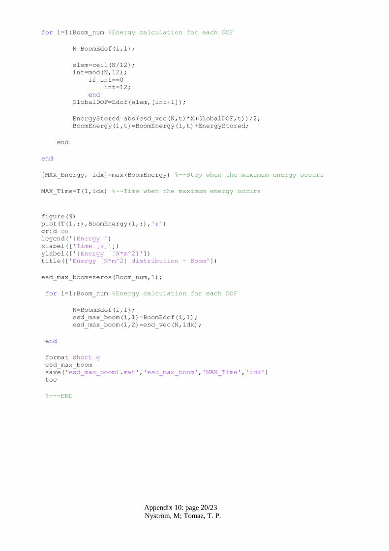
Appendix 10: page 20/23
Nyström, M; Tomaz, T. P.
for i=1:Boom_num %Energy calculation for each DOF
N=BoomEdof(i,1);
elem=ceil(N/12); int=mod(N,12); if int==0 int=12; end GlobalDOF=Edof(elem,[int+1]);
EnergyStored=abs(esd_vec(N,t)*X(GlobalDOF,t))/2; BoomEnergy(1,t)=BoomEnergy(1,t)+EnergyStored;
end
end
[MAX_Energy, idx]=max(BoomEnergy) %--Step when the maximum energy occurs
MAX_Time=T(1,idx) %--Time when the maximum energy occurs
figure(9) plot(T(1,:),BoomEnergy(1,:),'r') grid on legend('|Energy|') xlabel(['Time [s]']) ylabel(['|Energy| [N*m^2]']) title(['Energy [N*m^2] distribution - Boom'])
esd_max_boom=zeros(Boom_num,1);
for i=1:Boom_num %Energy calculation for each DOF
N=BoomEdof(i,1); esd_max_boom(i,1)=BoomEdof(i,1); esd_max_boom(i,2)=esd_vec(N,idx);
end
format short g esd_max_boom save('esd_max_boom1.mat','esd_max_boom','MAX_Time','idx') toc
%---END

Appendix 10: page 21/23
Nyström, M; Tomaz, T. P.
Code 5: beam3e_mod_3.m
function [Ke,Mec,Mel,fe]=beam3e(ex,ey,ez,eo,ep,eq) % Ke=beam3e(ex,ey,ez,eo,ep) % [Ke,fe]=beam3e(ex,ey,ez,eo,ep,eq) %---------------------------------------------------------------- % PURPOSE % Calculate the stiffness matrix for a 3D elastic Bernoulli % beam element. % % INPUT: ex = [x1 x2] % ey = [y1 y2] % ez = [z1 z2] node coordinates % % eo = [xz yz zz]; orientation of local z axis % % ep = [E G A Iy Iz Kv m J]; element properties % E: Young's modulus % G: Shear modulus % A: Cross section area % Iy: moment of inertia,local y-axis % Iz: moment of inertia,local z-axis % Kv: Saint-Venant's torsion constant % m: mass per length % J: polar moment of inertia % % eq = [qx qy qz qw]; distributed loads % % OUTPUT: Ke : beam stiffness matrix (12 x 12) % % Me : beam mass matrix (12 x 12) % % fe : equivalent nodal forces (12 x 1) %----------------------------------------------------------------- % LAST MODIFIED: E Serrano 1995-09-21 % Copyright (c) Division of Structural Mechanics and % Department of Solid Mechanics. % Lund Institute of Technology %-------------------------------------------------------------
b=[ ex(2)-ex(1); ey(2)-ey(1); ez(2)-ez(1) ]; L=sqrt(b'*b); n1=b/L;
lc=sqrt(eo*eo'); n3=eo/lc;
%
if nargin==5; eq=[0 0 0 0]; end
qx=eq(1); qy=eq(2); qz=eq(3); qw=eq(4); % E=ep(1); Gs=ep(2); A=ep(3); Iy=ep(4); Iz=ep(5); Kv=ep(6);%Ix m=ep(7);

Appendix 10: page 22/23
Nyström, M; Tomaz, T. P.
j=ep(8);
a=E*A/L ; b=12*E*Iz/L^3 ; c=6*E*Iz/L^2; d=12*E*Iy/L^3 ; e=6*E*Iy/L^2 ; f=Gs*Kv/L; g=2*E*Iy/L ; h=2*E*Iz/L ; cj=j/m/L;
Kle=[ a 0 0 0 0 0 -a 0 0 0 0 0 ; 0 b 0 0 0 c 0 -b 0 0 0 c ; 0 0 d 0 -e 0 0 0 -d 0 -e 0 ; 0 0 0 f 0 0 0 0 0 -f 0 0 ; 0 0 -e 0 2*g 0 0 0 e 0 g 0 ; 0 c 0 0 0 2*h 0 -c 0 0 0 h ; -a 0 0 0 0 0 a 0 0 0 0 0 ; 0 -b 0 0 0 -c 0 b 0 0 0 -c ; 0 0 -d 0 e 0 0 0 d 0 e 0 ; 0 0 0 -f 0 0 0 0 0 f 0 0 ; 0 0 -e 0 g 0 0 0 e 0 2*g 0 ; 0 c 0 0 0 h 0 -c 0 0 0 2*h]; % % % consistent mass matrix:
Mlec=(m*L/420)*[140 0 0 0 0 0 70 0 0 0 0 0; 0 156 0 0 0 22*L 0 54 0 0 0 -13*L; 0 0 156 0 -22*L 0 0 0 54 0 13*L 0; 0 0 0 140*cj 0 0 0 0 0 70*cj 0 0; 0 0 -22*L 0 4*L^2 0 0 0 -13*L 0 -3*L^2 0; 0 22*L 0 0 0 4*L^2 0 13*L 0 0 0 -3*L^2; 70 0 0 0 0 0 140 0 0 0 0 0 ; 0 54 0 0 0 13*L 0 156 0 0 0 -22*L; 0 0 54 0 -13*L 0 0 0 156 0 22*L 0; 0 0 0 70*cj 0 0 0 0 0 140*cj 0 0; 0 0 13*L 0 -3*L^2 0 0 0 22*L 0 4*L^2 0; 0 -13*L 0 0 0 -3*L^2 0 -22*L 0 0 0 4*L^2]; % % lumped mass matrix: mtot=(140+70+(156+54)*2)*2; s=(140+156+156)*2; Identity12=eye(12); Mlel=Identity12*Mlec*mtot/s; % fle=L/2*[qx qy qz qw -1/6*qz*L 1/6*qy*L qx qy qz qw 1/6*qz*L -
1/6*qy*L]';
% n2(1)=n3(2)*n1(3)-n3(3)*n1(2); n2(2)=-n1(3)*n3(1)+n1(1)*n3(3); n2(3)=n3(1)*n1(2)-n1(1)*n3(2); % An=[n1'; n2; n3]; % G=[ An zeros(3) zeros(3) zeros(3); zeros(3) An zeros(3) zeros(3); zeros(3) zeros(3) An zeros(3); zeros(3) zeros(3) zeros(3) An ]; %

Appendix 10: page 23/23
Nyström, M; Tomaz, T. P.
% Ke1=G'*Kle*G; Me1c=G'*Mlec*G; Me1l=G'*Mlel*G; fe1=G'*fle; %---------------------------------------------------------- if nargout==0 disp('Element stiffness matrix: '); disp(Ke1);
if nargin==6 disp('Element load vector: '); disp(fe1); end return end Ke=Ke1; Mec=Me1c; Mel=Me1l;
if nargin==6 fe=fe1; end %-------------------------- end -------------------------------


Faculty of Technology 351 95 Växjö, Sweden Telephone: +46 772-28 80 00, fax +46 470-832 17


![Fatigue Analysis [Compatibility Mode]](https://img.dokumen.tips/doc/110x75/577cc0c81a28aba7119117e8/fatigue-analysis-compatibility-mode.jpg)