Embed Size (px)
Citation preview

FATIGUE ANALYSIS OF 3D PRINTED 15-5 PH STAINLESS STEEL - A
COMBINED NUMERICAL AND EXPERIMENTAL STUDY
A Thesis
Submitted to the Faculty
of
Purdue University
by
Anudeep Padmanabhan
In Partial Fulfillment of the
Requirements for the Degree
of
Master of Science in Mechanical Engineering
August 2019
Purdue University
Indianapolis, Indiana

ii
THE PURDUE UNIVERSITY GRADUATE SCHOOL
STATEMENT OF COMMITTEE APPROVAL
Dr. Jing Zhang, Chair
Department of Mechanical and Energy Engineering
Dr. Andres Tovar
Department of Mechanical and Energy Engineering
Dr. Xiaoliang Wei
Department of Mechanical and Energy Engineering
Approved by:
Dr. Jie Chen
Head of the Graduate Program

iii
To, my wife, the source of my strength
my parents, for their unwavering support
my brother, for his belief in me
my friends, for making my life easier
and to the guiding hand, taking me to my best

iv
ACKNOWLEDGMENTS
I would like to acknowledge the immense support provided to me by Dr. Zhang
without who’s constant encouragement, I would not have achieved this result. He pro-
vided me with unequivocal support to achieve my goals and was patient through my
errors. His constant encouragement helped me get the National Science Foundation
grant and helped me present papers in several conferences of repute.
I would like to thank Dr. Andres Tovar and Dr. Xiaoliang Wei for their support
during my time at the university and for serving as part of my advisory committee.
I would like to thank the support provided by Walmart foundation grant ti-
tled, “Optimal Plastic Injection Molding Tooling Design and Production through
Advanced Additive Manufacturing”, and 3D parts MFG,LLC for 3D printing of the
fatigue samples.
I would like to thank my lab mates, Sugrim Sagar, Nishant Hawaldar, Abhilash
Gulhane, Xuehui Yang, Lingin Meng among others for all their help and banter.
Last, but not the least, I would like to thank my wife, parents, brother and friends
for always standing by my side.

v
TABLE OF CONTENTS
Page
LIST OF TABLES . . . . . . . . . . . . . . . . . . . . . . . . . . . . . . . . . . vii
LIST OF FIGURES . . . . . . . . . . . . . . . . . . . . . . . . . . . . . . . . . viii
ABSTRACT . . . . . . . . . . . . . . . . . . . . . . . . . . . . . . . . . . . . . x
1 INTRODUCTION . . . . . . . . . . . . . . . . . . . . . . . . . . . . . . . . 1
1.1 Motivation . . . . . . . . . . . . . . . . . . . . . . . . . . . . . . . . . . 1
1.2 Objective . . . . . . . . . . . . . . . . . . . . . . . . . . . . . . . . . . 2
1.3 Structure of the Thesis . . . . . . . . . . . . . . . . . . . . . . . . . . . 2
2 LITERATURE REVIEW . . . . . . . . . . . . . . . . . . . . . . . . . . . . 4
2.1 Additive Manufacturing . . . . . . . . . . . . . . . . . . . . . . . . . . 4
2.2 Fatigue, Plasticity and Damage . . . . . . . . . . . . . . . . . . . . . . 4
2.2.1 Fatigue Modelling . . . . . . . . . . . . . . . . . . . . . . . . . . 5
2.2.2 Modelling Plasticity . . . . . . . . . . . . . . . . . . . . . . . . 9
2.2.3 Representation of Damage . . . . . . . . . . . . . . . . . . . . . 16
2.2.4 Implementation of the Constitutive Model in FE Tool . . . . . . 22
2.2.5 Procedure for Determination of Material Parameters . . . . . . 24
2.3 Direct Cyclic Method . . . . . . . . . . . . . . . . . . . . . . . . . . . . 26
2.3.1 Need for a Quasi-static Approach . . . . . . . . . . . . . . . . . 26
2.3.2 Implementation in FE Model . . . . . . . . . . . . . . . . . . . 28
2.3.3 Solution Accuracy . . . . . . . . . . . . . . . . . . . . . . . . . 29
3 EXPERIMENTAL PROCEDURE . . . . . . . . . . . . . . . . . . . . . . . . 32
3.1 Preparation of Specimen . . . . . . . . . . . . . . . . . . . . . . . . . . 32
3.2 Fatigue Testing of Specimen . . . . . . . . . . . . . . . . . . . . . . . . 34
3.3 Results and Discussion . . . . . . . . . . . . . . . . . . . . . . . . . . . 35
4 NUMERICAL MODELLING . . . . . . . . . . . . . . . . . . . . . . . . . . 37
vi
Page
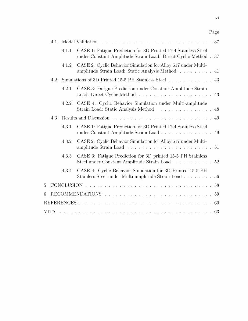
4.1 Model Validation . . . . . . . . . . . . . . . . . . . . . . . . . . . . . . 37
4.1.1 CASE 1: Fatigue Prediction for 3D Printed 17-4 Stainless Steelunder Constant Amplitude Strain Load: Direct Cyclic Method . 37
4.1.2 CASE 2: Cyclic Behavior Simulation for Alloy 617 under Multi-amplitude Strain Load: Static Analysis Method . . . . . . . . . 41
4.2 Simulations of 3D Printed 15-5 PH Stainless Steel . . . . . . . . . . . . 43
4.2.1 CASE 3: Fatigue Prediction under Constant Amplitude StrainLoad: Direct Cyclic Method . . . . . . . . . . . . . . . . . . . . 43
4.2.2 CASE 4: Cyclic Behavior Simulation under Multi-amplitudeStrain Load: Static Analysis Method . . . . . . . . . . . . . . . 48
4.3 Results and Discussion . . . . . . . . . . . . . . . . . . . . . . . . . . . 49
4.3.1 CASE 1: Fatigue Prediction for 3D Printed 17-4 Stainless Steelunder Constant Amplitude Strain Load . . . . . . . . . . . . . . 49
4.3.2 CASE 2: Cyclic Behavior Simulation for Alloy 617 under Multi-amplitude Strain Load . . . . . . . . . . . . . . . . . . . . . . . 51
4.3.3 CASE 3: Fatigue Prediction for 3D printed 15-5 PH StainlessSteel under Constant Amplitude Strain Load . . . . . . . . . . . 52
4.3.4 CASE 4: Cyclic Behavior Simulation for 3D Printed 15-5 PHStainless Steel under Multi-amplitude Strain Load . . . . . . . . 56
5 CONCLUSION . . . . . . . . . . . . . . . . . . . . . . . . . . . . . . . . . . 58
6 RECOMMENDATIONS . . . . . . . . . . . . . . . . . . . . . . . . . . . . . 59
REFERENCES . . . . . . . . . . . . . . . . . . . . . . . . . . . . . . . . . . . . 60
VITA . . . . . . . . . . . . . . . . . . . . . . . . . . . . . . . . . . . . . . . . . 63

vii
LIST OF TABLES
Table Page
2.1 Figure 2.1 values [8] . . . . . . . . . . . . . . . . . . . . . . . . . . . . . . 6
2.2 Stress regime for Bree diagram [20] . . . . . . . . . . . . . . . . . . . . . . 14
3.1 Chemical composition of 3D printed 15-5 PH stainless steel [32]. . . . . . . 32
3.2 Fatigue result tabulation . . . . . . . . . . . . . . . . . . . . . . . . . . . . 35
4.1 Backstresses Ci and γi values for 3D printed 17-4 stainless steel . . . . . . 40
4.2 Damage parameters for 3D printed 17-4 stainless steel . . . . . . . . . . . 40
4.3 Kinematic hardening parameters for Alloy 617 [35] . . . . . . . . . . . . . 42
4.4 Isotropic hardening parameters for Alloy 617 [35] . . . . . . . . . . . . . . 43
4.5 Kinematic hardening evolution parameters [35] . . . . . . . . . . . . . . . . 43
4.6 Backstresses Ci and γi values for 3D printed 15-5 PH stainless steel . . . . 45
4.7 Damage parameters for 3D printed 15-5 PH stainless steel . . . . . . . . . 47
4.8 Coffin-Mason-Basquin parameters for 3D printed 15-5 PH stainless steel . 54

viii
LIST OF FIGURES
Figure Page
2.1 Pie chart representation of causes of structural failure [8] . . . . . . . . . . 5
2.2 Crack growth rate as a function of K [15] . . . . . . . . . . . . . . . . . . . 8
2.3 Isotropic hardening surface evolution [18] . . . . . . . . . . . . . . . . . . . 10
2.4 Kinematic hardening yield surface evolution [18] . . . . . . . . . . . . . . . 11
2.5 Bauschinger effect [19] . . . . . . . . . . . . . . . . . . . . . . . . . . . . . 12
2.6 Stress-strain curve with ratcheting phenomenon [18] . . . . . . . . . . . . . 12
2.7 Bree diagram showing stress regimes [20] . . . . . . . . . . . . . . . . . . . 13
2.8 Stress and plastic strain for half cycle of regime R1 [20] from figure 2.7 . . 14
2.9 Monotonic and cyclic plastic strain threshold [23] . . . . . . . . . . . . . . 21
2.10 Calculating damage initiation parameters C1 and C2 from hysteresis en-ergy [27] . . . . . . . . . . . . . . . . . . . . . . . . . . . . . . . . . . . . . 25
2.11 Calculating damage evolution parameters C3 and C4 [27] . . . . . . . . . . 26
2.12 Methodology incorporated by Dang et al. [28] . . . . . . . . . . . . . . . . 27
2.13 Comparison of stabilized cycle obtained by direct method with static cy-cling method . . . . . . . . . . . . . . . . . . . . . . . . . . . . . . . . . . 29
2.14 Convergence study for damage parameter . . . . . . . . . . . . . . . . . . 30
3.1 SEM image of 15-5 PH powder [34] . . . . . . . . . . . . . . . . . . . . . . 33
3.2 15-5 PH rotating bending specimen . . . . . . . . . . . . . . . . . . . . . . 33
3.3 Functioning of MT3120 [33] . . . . . . . . . . . . . . . . . . . . . . . . . . 34
3.4 MT3210 Fatigue tester [33] . . . . . . . . . . . . . . . . . . . . . . . . . . . 34
3.5 Result of the fatigue test . . . . . . . . . . . . . . . . . . . . . . . . . . . . 35
3.6 The specimen after fatigue failure . . . . . . . . . . . . . . . . . . . . . . . 36
3.7 Complimentary specimen surfaces after fatigue failure . . . . . . . . . . . . 36
4.1 FE model for axial Tension-compression fatigue test specimen . . . . . . . 38

ix
Figure Page
4.2 Load function . . . . . . . . . . . . . . . . . . . . . . . . . . . . . . . . . . 38
4.3 Material characterization for 17-4 [6] . . . . . . . . . . . . . . . . . . . . . 39
4.4 Regression fit for damage evolution . . . . . . . . . . . . . . . . . . . . . . 40
4.5 Multi-amplitude strain . . . . . . . . . . . . . . . . . . . . . . . . . . . . . 41
4.6 FE model for the rotary fatigue specimen . . . . . . . . . . . . . . . . . . 44
4.7 Experimentally measured uniaxial tension Stress-strain graph for 3D printed15-5 PH stainless steel . . . . . . . . . . . . . . . . . . . . . . . . . . . . . 45
4.8 Curve fit applied to experimental data . . . . . . . . . . . . . . . . . . . . 46
4.9 Total backstress(solid line) and it’s decomposed components . . . . . . . . 46
4.10 Damage evolution parameter fit . . . . . . . . . . . . . . . . . . . . . . . . 47
4.11 Multi-amplitude strain for CASE 4 . . . . . . . . . . . . . . . . . . . . . . 48
4.12 Family of cyclic stress-strain curves for different strain ranges . . . . . . . 49
4.13 Normalised damage vs cycles . . . . . . . . . . . . . . . . . . . . . . . . . 50
4.14 Strain life curve for vertically printed as built 17-4 stainless steel . . . . . . 50
4.15 Comparison of FEA result with literature [35] . . . . . . . . . . . . . . . . 51
4.16 Variation of stress-strain loops for different strain range . . . . . . . . . . . 52
4.17 Variation of damage parameter with cycles for different strain ranges . . . 53
4.18 Comparison of strain life curve between fit data and FEA . . . . . . . . . . 53
4.19 Comparison between experimental data and Coffin-Manson-Basquin pre-diction for 3D printed 15-5 PH stainless steel . . . . . . . . . . . . . . . . . 54
4.20 Von Mises stress plots for the model at different cycles with damagedmaterial at 65th cycle . . . . . . . . . . . . . . . . . . . . . . . . . . . . . 55
4.21 Damage parameter at different cycles with damaged material at 65th cycle 55
4.22 Cycle dependent stress variation . . . . . . . . . . . . . . . . . . . . . . . . 56
4.23 Stress-strain curve . . . . . . . . . . . . . . . . . . . . . . . . . . . . . . . 57

x
ABSTRACT
Padmanabhan, Anudeep. M.S.M.E., Purdue University, August 2019. Fatigue Analy-sis of 3D Printed 15-5 PH Stainless Steel - A Combined Numerical and ExperimentalStudy. Major Professor: Jing Zhang.
Additive manufacturing (AM) or 3D printing has gained significant advancement
in recent years. However the potential of 3D printed metals still has not been fully
explored. A main reason is the lack of accurate knowledge of the load capacity of 3D
printed metals, such as fatigue behavior under cyclic load conditions, which is still
poorly understood as compared with the conventional wrought counterpart.
The goal of the thesis is to advance the knowledge of fatigue behavior of 15-5
PH stainless steel manufactured through laser powder bed fusion process. To achieve
the goal, a combined numerical and experimental study is carried out. First, using
a rotary fatigue testing experiment, the fatigue life of the 15-5 PH stainless steel
is measured. The strain life curve shows that the numbers of the reversals to fail-
ure increase from 13,403 to 46,760 as the applied strain magnitudes decrease from
0.214% from 0.132%, respectively. The microstructure analysis shows that predomi-
nantly brittle fracture is presented on the fractured surface. Second, a finite element
model based on cyclic plasticity including the damage model is developed to predict
the fatigue life. The model is calibrated with two cases: one is the fatigue life of 3D
printed 17-4 stainless steel under constant amplitude strain load using the direct cyclic
method, and the other one is the cyclic behavior of Alloy 617 under multi-amplitude
strain loads using the static analysis method. Both validation models show a good
correlation with the literature experimental data. Finally, after the validation, the
finite element model is applied to the 15-5 PH stainless steel. Using the direct cyclic
method, the model predicts the fatigue life of 15-5 PH stainless steel under constant
xi
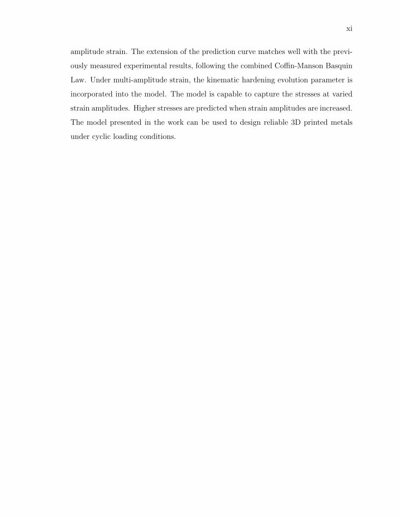
amplitude strain. The extension of the prediction curve matches well with the previ-
ously measured experimental results, following the combined Coffin-Manson Basquin
Law. Under multi-amplitude strain, the kinematic hardening evolution parameter is
incorporated into the model. The model is capable to capture the stresses at varied
strain amplitudes. Higher stresses are predicted when strain amplitudes are increased.
The model presented in the work can be used to design reliable 3D printed metals
under cyclic loading conditions.

1
1. INTRODUCTION
The field of 3D printing technology is vast, but novel. The widespread acceptance to-
wards the additive manufacturing technology has pushed the pace for standardization
of the process. This is necessary to develop engineering confidence in the material
and the process. The advantages provided by 3D printing has made it possible for it
to be overarching across many fields.
3D printing technology started out as a way to prototype designs for testing. The
additive manufacturing process quickly took a more meaningful role as it’s benefits
were realized. As 3D printing methodology took a mainstream path, there generated
a need for understanding and characterizing the various material properties associated
with a engineering usage. It’s extensive usage in design of engineering components
necessitated a need to develop predictive models to determine the material behavior
of 3D printed specimen.
1.1 Motivation
Additive manufacturing (AM) or 3D printing process has made rapid strides in
recent years. However, the full potential of 3D printing technology hasn’t been rig-
orously explored. There is still a dearth of knowledge about it’s mechanical abilities,
such as the fatigue behavior under cyclic load conditions. Further still, there is a
lack of characterization for a numerical model to predict their mechanical behavior
as compared to their wrought counterparts.
There are many methods to assess the fatigue life of structures. Most commonly,
one uses the S-N curves for assessing component life. The standard fatigue prediction
methods have a linear damage approach. The research conducted in fracture mechan-
ics have established that such an approach is conservative with studies conducted for

2
the establishment of Paris law [1]. Moreover, there is no information about damage or
crack behavior with these approaches. The increasing usage of 3D printed materials
in high energy applications has made it critical to have a characterized numerical
model which would incorporate non-linearity for damage or crack evolution. To un-
derstand the cyclic behavior of 3D printed parts and to characterize the parameters
associated with cyclic behavior leading to fatigue would further accelerate acceptance
of additive manufacturing process.
1.2 Objective
The goal of the thesis is to advance the knowledge of fatigue behavior of 15-5
PH stainless steel manufactured through laser powder bed fusion process. This is
done through a combined numerical and experimental study. First, using a rotary
fatigue testing experiment, the fatigue life of the 15-5 PH stainless steel is measured.
Second, a finite element model based on cyclic plasticity, including the damage model,
is developed to predict the fatigue life. Finally, after model validation, the finite
element model is applied to the 15-5 PH stainless steel.
1.3 Structure of the Thesis
This thesis is divided into five sections. The first is the introduction which would
cover the motivation, objective and the overall structure of thesis.
The second chapter reviews literature that is relevant to characterization of the
cyclic and fatigue properties. It contains an overview of existing works characterizing
cyclic 3D printed material properties. Then the concept of fatigue, plasticity and
damage mechanics is introduced. These directly relate to material characterization.
The third chapter deals with the experimental procedure that was carried out.
The 3D printing process to produce the test specimen and the testing methodology
for fatigue are briefly discussed.

3
The fourth chapter models the cyclic behavior utilizing a finite element tool. The
modelling technique employed is discussed. Two calibration simulations are carried
out to show model viability and then the said model is applied to develop a predic-
tive model for 3D printed 15-5 PH Stainless steel. The results of the approach are
discussed.
The fifth chapter would conclude the findings of this study and the sixth chapter
would recommend future work associated with the finite element model.
4
2. LITERATURE REVIEW
2.1 Additive Manufacturing
Research into the material behavior of 3D printed parts has been going on for
decades. Understanding the fatigue behavior of component is critical and to this
end, many publications have focused on determining such properties. Sehrt et al. [2]
was one of the first to investigate the dynamic properties of 3D printed parts as
they determined the fatigue strength of SLM built 17-4 PH stainless steel. They
investigated the effect of orientation on the fatigue life. Spierings et al. has conducted
numerous investigations [3] [4] [5] to assess the effect of manufacturing parameters on
mechanical property, including fatigue life.
Numerical modelling of 3D printed specimen has picked up in the last two years. A
similar experiment to the one by Sehrt [2] was conducted more recently by Yadollahi
[6] where they characterized the cyclic behavior of 17-4 PH stainless steel with a cyclic
Ramberg-Osgood model. They extended this characterization to encompass their
dependence on printing orientation. Similar characterization was done for the 3D
printed AISI 18Ni30 [7] where the low cycle fatigue characteristics were investigated
and fit to Coffin-Manson curve.
2.2 Fatigue, Plasticity and Damage
Throughout history, engineers have worked towards understanding the phenomenon
of failure of structures or mechanical parts. It began with the conceptual study of
stress and strain and how one could measure failure using these two parameters.
Many theories of failure were proposed.

5
Theories on failure can be broadly classified into macroscopic failures and mi-
croscopic failures criteria. The macroscopic criteria usually takes into account the
macroscopic effects of stress and strain and include failure theories like von Mises
theory, Maximum principal stress theory among others. This approach sticks to the
elastic regime and doesn’t take into account the toughness of the material after it
yields.
The microscopic failure criteria leverages the theories of fracture mechanics and
continuum mechanics. These theories are more robust from a theoretical point of
view because the mechanism defining failure is explored in detail. They see failures,
in this case crack propagation, as irreversible thermodynamic processes and thus can
be defined using energy conservation principles.
2.2.1 Fatigue Modelling
Fig. 2.1. Pie chart representation of causes of structural failure [8]
The term ’Fatigue’ was first introduced to mean failure due to repeated cycles of
loading, in the middle of 19th century, by J.B.Poncelet [8]. It took the initial works of
Wohler, who was an engineer investigating the failure of railroad axles (particularly
6
the Versailles accident [9] which gave the impetus to this research), to convince the
engineers about failures occurring below the monotonic failure limit of the material.
This gave rise to S − N curves, also called Wohler curves, that are still used today
to predict the fatigue life of material. It was soon to be understood that the primary
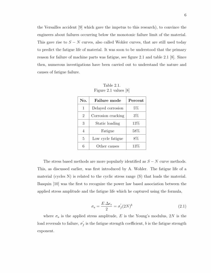
reason for failure of machine parts was fatigue, see figure 2.1 and table 2.1 [8]. Since
then, numerous investigations have been carried out to understand the nature and
causes of fatigue failure.
Table 2.1.Figure 2.1 values [8]
No. Failure mode Percent
1 Delayed corrosion 5%
2 Corrosion cracking 3%
3 Static loading 13%
4 Fatigue 58%
5 Low cycle fatigue 8%
6 Other causes 13%
The stress based methods are more popularly identified as S −N curve methods.
This, as discussed earlier, was first introduced by A. Wohler. The fatigue life of a
material (cycles N) is related to the cyclic stress range (S) that loads the material.
Basquin [10] was the first to recognize the power law based association between the
applied stress amplitude and the fatigue life which he captured using the formula,
σa =E.∆εe
2= σ
′
f (2N)b (2.1)
where σa is the applied stress amplitude, E is the Young’s modulus, 2N is the
load reversals to failure, σ′
f is the fatigue strength coefficient, b is the fatigue strength
exponent.

7
Palmgren-Miner introduced the linear cumulative damage hypothesis which ap-
plied the S-N curve for variable amplitude loading. This is popularly called the
Miner’s rule [11] and is given by,
n∑i=1
niNi
= 1 (2.2)
where, ni is the number of cycles the material was subjected to at stress σi, Ni is the
number of reversals to failure at stress level σi.
The material is assumed to have failed when the cumulative damage at different
stress amplitude σi reaches 1. This method was further improved by Goodman,
Soderberg and Gerber who introduced the effect of stress ratio and mean stresses on
the fatigue life through their respective criteria.
For components subjected to cyclic loads that induce plasticity in the very first
cycle, the fatigue life is affected by plastic strains. In this type of loading, it makes
more sense for us to define the life of material using the strains as they can be
differentiated into plastic and elastic components. This gave rise to strain based
fatigue assessments. The relationship, similar to the Basquin relationship, is famously
given by Coffin-Manson [12] [13] [14] as,
εp2
= ε′
f (2N)c (2.3)
where, εp/2 is the plastic strain amplitude, ε′
f is the fatigue ductility co-efficient and
c is the fatigue ductility exponent.
The two models shown by eq.2.1(elastic) and eq.2.3(plastic) are combined and the
consolidated total strain to life relationship [14] given as,
∆εT2
= εa =εe2
+εp2
=σ′
f
E(2N)b + ε
′
f (2N)c (2.4)
Continuum damage mechanics based approach is a relatively new methodology
that posits that strain energy release is the major contributor towards the fatigue fail-
ure of materials. This method has been heavily researched beginning with Kachanov

8
then improved by Chaboche and Lemaitre. This method and fracture mechanics
based approaches to fatigue rely on power law based representation of crack propa-
gation.
The continuum mechanics based approach will be discussed in detail in the coming
sections. The crack propagation theory is mainly based on Paris law [1] which gives
the rate of crack growth as,
da
dN= A(∆K)n where ∆K = Y∆σ
√πa (2.5)
where, A and n are constants for materials and Y is geometry factor depending on
mode of loading. K is the stress intensity factor.
The crack propagation was better understood later as having non-linearity. Then
three regions describing crack growth was mooted which is seen in fig.2.2.
Fig. 2.2. Crack growth rate as a function of K [15]
9
2.2.2 Modelling Plasticity
Before a ductile material fails, it goes through the process of yielding. This be-
havior is non-linear such that it is difficult to assign a modulus to predict the loading
path. The accurate modelling of this effect is an important tool to understand the
evolution of Continuum damage mechanics. This theory primarily relies on the accu-
mulated plastic strains and strain energy density concepts to capture fatigue damage
accumulation. A brief summary is provided here.
Elastic deformations are reversible. When a material is loaded beyond it’s elastic
limit, it undergoes irreversible deformation. On unloading we recover the elastic part
of the deformation. The behavior of the material is linear in the elastic zone and
becomes non-linear once it crosses the yield point.
As the material crosses yield point, it experiences a coalescence of defects causing
a temporary saturation. This makes the material more resistant to deformation and
thus can be said to have hardened. This is called strain hardening process.
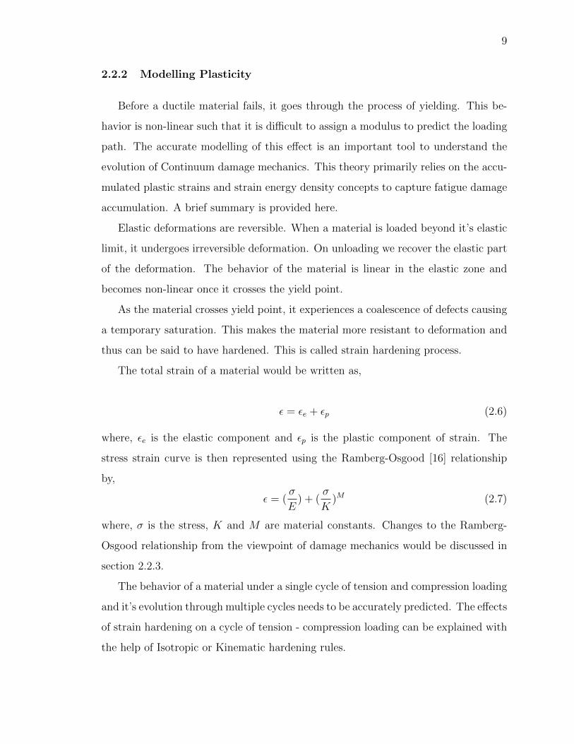
The total strain of a material would be written as,
ε = εe + εp (2.6)
where, εe is the elastic component and εp is the plastic component of strain. The
stress strain curve is then represented using the Ramberg-Osgood [16] relationship
by,
ε = (σ
E) + (
σ
K)M (2.7)
where, σ is the stress, K and M are material constants. Changes to the Ramberg-
Osgood relationship from the viewpoint of damage mechanics would be discussed in
section 2.2.3.
The behavior of a material under a single cycle of tension and compression loading
and it’s evolution through multiple cycles needs to be accurately predicted. The effects
of strain hardening on a cycle of tension - compression loading can be explained with
the help of Isotropic or Kinematic hardening rules.

10
In Isotropic hardening, it is assumed that the yield surface of the material would
remain the same shape. If a function F (σij, K) describing the yield surface of a
material under hardening effect is written as [17],
F (σij, Ki) = 0 (2.8)
where, σij is the stress tensor, Ki represents strain hardening parameters, then ac-
cording to isotropic hardening rule the yield surface changes as such that [17],
F (σij, Ki) = f0(σij)−K = 0 (2.9)
which shows that the function has changed only by expansion and hasn’t changed
in shape. The figure 2.3 shows material under a tension-compression loading cycle
following the isotropic hardening rule. As seen, the new yield surface is a scaling of
the original by kinematic hardening factor. One important implication of this rule is
that the yield in tension and compression would be same. This is not true for most
materials.
Fig. 2.3. Isotropic hardening surface evolution [18]

11
Kinematic hardening rule states that the yield surface of the material translates
under reversed loading regime. Taking the same yield function, 2.8, the modified
yield function for kinematic hardening rule would be [17],
F (σij, Ki) = F (σij − αij) = 0 (2.10)
where the hardening parameter, αij is called backstress. Figure 2.4 shows that the
Fig. 2.4. Kinematic hardening yield surface evolution [18]
yield surface has neither changed it’s shape or size but has shifted by the hardening
parameter(backstress),αij. The implication of this rule is that the yield point in
tension would not be the same as that in compression.
Upon unloading and subsequent compressive loading we see that the yield in
compression is less than the yield point in tension. This weakening of material is
referred to as Bauschinger effect [19].
In the figure 2.5, O represents the zero stress state, OAB is the loading path the
material takes under tension, BC is the unloading stage, CDE is the loading path
under compression and EF is the subsequent relaxation. We observe that for most
materials, it follows the kinematic hardening path because of which the yield point
in tension is less than that in compression(σyp < σ′yp).

12
Fig. 2.5. Bauschinger effect [19]
When the material is subjected to cyclic loading, it experiences the hardening
effects across multiple cycles as well as within a single cycle. The material can ac-
cumulate strains over the span of cycles which essentially means that the cyclic load
creates open elasto-plastic loops. Under stress-controlled tests with unsymmetrical
loads, we observe that the strains continue to increase cycle by cycle in the direction
of unsymmetry.
Fig. 2.6. Stress-strain curve with ratcheting phenomenon [18]

13
The plastic strains keep accumulating and we observe a phenomenon called ratch-
eting, otherwise known as cyclic creep. This is usually characterized by a shifting
hysteresis loop. Fig 2.6 shows the gradual accumulation of strains across multiple
loops. The hardening models proposed previously could capture the behavior of
single cycle but couldn’t predict cyclic phenomenon like cyclic hardening/softening,
shakedown or ratcheting. This phenomenon was first categorized by Bree [20] when
he tried to explain the thinning of nuclear fuel cans. These components were loaded
with pressure internally, were subjected to thermal fluctuations and experienced un-
symmetric load cycles. The Bree diagrams were a way for predicting the ratcheting
phenomenon. Ratcheting can severely affect the life of components subjected to cyclic
loading.
Fig. 2.7. Bree diagram showing stress regimes [20]
14
Table 2.2.Stress regime for Bree diagram [20]
Stress regime Can behavior
R1 and R2 Ratchetting
S1 and S2 Shakedown after first half cycle
P Plastic cycling
E Elastic
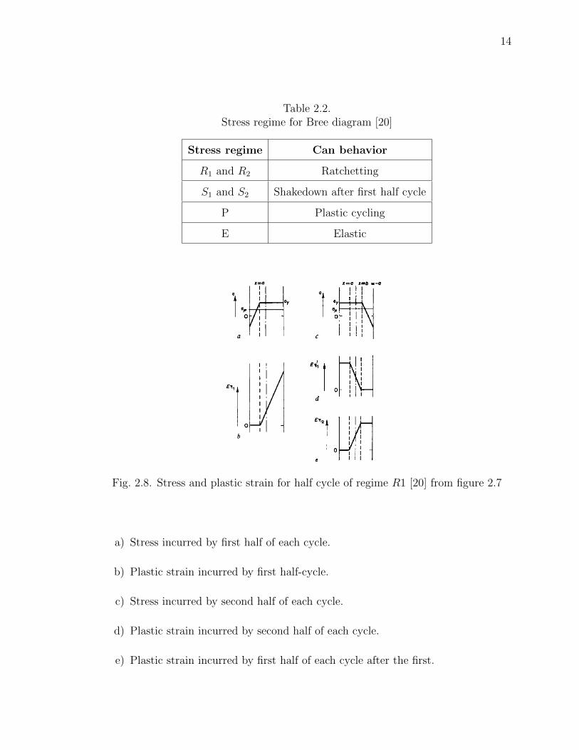
Fig. 2.8. Stress and plastic strain for half cycle of regime R1 [20] from figure 2.7
a) Stress incurred by first half of each cycle.
b) Plastic strain incurred by first half-cycle.
c) Stress incurred by second half of each cycle.
d) Plastic strain incurred by second half of each cycle.
e) Plastic strain incurred by first half of each cycle after the first.

15
The methodologies mentioned above were the first attempts to characterize the
cyclic material behavior. The Bree model was considered conservative and efforts to
better the model were made. There was a need for a non-linear kinematic/isotropic
(combined) hardening (NLKH) model which would be defined as,
F (σij, Ki) = F (σij − αij)−K = 0 (2.11)
Frederick-Armstrong model [21] is one of the first to predict ratcheting by pre-
dicting backstress with,
dα =C
σ0dp− γ.α.dp (2.12)
where, C and γ are material constants to be calibrated and α is the backstress after
varying yield limit σ0 (see equation 2.16) for the plastic strain p. The Chaboche
model [18] improved this by generalizing the net as a summation of multiple back-
stress to capture realistic shapes of stress-strain curve, giving
dα =n∑i
Ciσ0
(σ − α)dp− γi.αi.dp (2.13)
It is to be noted that Ci and γi are not be considered as material parameters but rather
as series decomposition of a simpler expression, for instance, by a power law [18]. The
integration of 2.13 would give the monotonic stress-strain curve
σ(p) = σ0 +n∑i
Ciγi
(1− e−γip) (2.14)
which when further integrated for cyclic stress-strain curve from stabilized cycle gives,
∆σ(∆p)
2= σ0 +
n∑i
Ciγi
tanh γi∆p
2(2.15)
where the ∆σ represents the cyclic stress amplitude range for plastic amplitude ∆p
With addition of isotropic hardening effect, it is understood that the yield surface
in equation 2.15 expands as plastic loading continues. Thus, σ0 varies as,

16
σ0 = k +R
and R = Q(1− e−bp)(2.16)
where k is the initial yield stress of the material during the first half of the first cycle.
Q and b are isotropic hardening constants.
The above equation captures the phenomenon of cyclic hardening/softening more
accurately. Further, the model could be made sensitive to the variation of γi to plastic
strain component and have it vary with [22],
γi = γi,ini +k∑i=1
Li(1− e−dip) (2.17)
where γi,ini is the γ value at first cycle. Li and di are kinematic hardening evolution
parameters.
2.2.3 Representation of Damage
Damage is a process by which the material loses it’s load carrying capacity and
ultimately results in breaking of the part. Lemaitre [23] classifies the types of damage
variables and their applicability by scale. Damage, at the microscale level, is the
concentration of microstresses around defects or interfaces, both of which results in
deterioration of material. At the mesoscale level we have to look at the concept of
’Representative Volume Element’(RVE) which is an abstract volume capturing the
effects of microscale and translating it into mesoscale without smoothing the high
gradients. At this scale, crack is initiated by the coalescing of voids or defects. At the
macroscale level, this manifests as growth of crack. The first two stages are modeled
using the theory of continua while the third stage is studied using fracture mechanics.
We now shall delve into the evolution of this concept.
The first instance of a damage parameter used was in the works of Kachanov [24] to
model effects of material deterioration under creep conditions. In his works, Kachanov
introduced the concept as the ’continuing parameter’,ψ, with

17
0 ≤ ψ ≤ 1 (2.18)
such that ψ = 1 represents the condition of undamaged state or virgin material. The
material is understood to undergo deterioration as ψ decreases.
Let us consider a damaged material. An RVE is cut out of the bulk with its
normal, #»n and let δS be the cross-sectional area of the RVE and δSDs be the total
area of microvoids and cracks on δS. Also defining damage parameter D( #»n, s) with
plane s as (see Lemaitre, [23]),
D = 1− ψ (2.19)
and
D( #»n, s) =δSDsδS
(2.20)
To get the parameter to be continuous, we take the plane s where the damage is
maximum, such that the parameter loses it’s dependency on plane,
D( #»n ) =δSDδS
(2.21)
A kinetic equation for ψ was developed as,
dψ
dt= F (ψ, σij, ..), ψ = 1 at t = 0 (2.22)
under simplified conditions, F = F (σmax
ψ), where σmax is the maximum tensile stress
at a given point. Kachanov further suggested a power law to represent F.
dψ
dt= −A(
σmaxψ
)n (2.23)
Kachanov’s theory didn’t couple the phenomenon of creep and damage accumula-
tion. Thus it was modified by Rabotnov [25] by first suggesting additional parameters
to capture this effect. This was to be fit by using experimental results. But the main
contribution was to directly associate the damage parameter to stresses in material.
Let the RVE be acted upon by a force#»
F = #»nF , inducing an uniaxial stress
σ =
#»
F
S=
#»nF
S(2.24)
18
Assuming that no forces are effected by the microvoids and cracks, and that the
effective area has been reduced to S − SD, the effective stress, σ is given as,
σ =
#»
F
S − SD(2.25)
It can also be written as,
σ =
#»
F
S(1− SD
S)or σ =
σ
1−D(2.26)
where D = SD
Sis the damage variable. Here it is assumed that the behavior of
microvoids and/or cracks is same in tension as in compression, which is not the case
in practice. Also, material is assumed to be isotropic and the load is considered to be
uniaxial. Thus this theory is limited to cases where the compressive loads are small.
Lemaitre [23] proposed that, “The strain behavior of a damaged material is rep-
resented by constitutive equations of a virgin material(without any damage) in the
potential of which the stress is simply replaced with effective stress”. Thus,
εe =σ
E=
σ
(1−D)E(2.27)
where, εe is the elastic strain and E is the Young’s modulus of the material. Also,
the Ramberg-Osgood relation [16] for plastic strain changes to
ε = (σ
E) + (
σ
K∗)M∗
(2.28)
where, ε is the total strain, K∗ and M∗ are material constants.
Assuming small deformation loads, the total strain can be split into two parts, a
thermo-elastic part εe and a plastic part εp, giving
εij = εeij + εpij (2.29)
The Helmholtz specific free energy is a function of parameters affecting the stress-
strain curve, including damage. Let us consider this measure with ψ(εij, D, etc., ). It
can be argued that this too would have a distinct elastic and plastic components. It
is more convenient to use the Gibb’s specific free enthalpy(ψ∗) here such that [23],

19
ψ∗ = ψ∗e +1
ρσijε
pij − ψp − ψT , (2.30)
where, the thermal component ψT is not considered further in this work, and ψp =
1ρ(r∫0
Rdr+ 13Cαijαij) is the contribution from plastic hardening. Multiplied by density
ρ it is energy stored ws in the RVE. Another important point is to observe that
the term ψ∗e ensures coupling between elasticity and damage through effective stress
concept discussed earlier.
The state laws derived from this formalism are,
εij = ρ∂ψ∗
∂σij
R = −ρ∂ψ∗
∂r,
Xij = −ρ ∂ψ∗
∂αij
Y = −ρ∂ψ∗
∂D
(2.31)
The kinetic laws for evolution of these internal variables are derived from a dissi-
pation potential (F ) which is written as [23],
F = F (σ,R,Xij, Y ;Detc., ) (2.32)
This potential can be split into components like plastic criterion (f), non-linear
kinematic hardening term (FX) and damage potential (FD). The evolution laws are
written as the contributing component derivative with a time dependent variable.
˙εpij = λ∂F
∂σij
r = −λ∂F∂R
αij = −λ ∂F
∂Xij
D = λ∂F
∂Y
(2.33)
The components of evolution laws are incorporated along with the principle of strain
equivalence, and the thermo-elastic law thus derived from the strain potential is,

20
εeij =1 + ν
Eσij −
ν
Eσkkδij (2.34)
where the effective stress is σij = σij1−D . The energy density release rate, associated
with damage can be written as,
Y =˜σ2eqRν
2E(2.35)
and the triaxiality function,
Rν =2
3(1 + ν) + 3(1− 2ν)(
σHσeq
2
) (2.36)
where σH = σkk/3 is the hydrostatic stress, σeq =√
32σDijσ
Dij the von Mises equivalent
stress. The derivations are curtailed for the sake of brevity, a detailed discussion
could be obtained from Lemaitre’s book [23].
Damage Initiation
The materials exhibit a certain resistance for damage initiation during plastic
loading or fatigue. There is a threshold associated with stored energy (wD) required
for the defects to coalesce. From the different hardening and elasto-plasticity laws we
can define stored energy as [23],
ws =
t∫0
(Rr +Xijαij)dt (2.37)
Consider the associated plastic strain ps and threshold plastic strain pD. It is
shown that the isotropic hardening saturates at the value R = R∞ for large p and
we know that p = r for D = 0 and also recall the state laws from which we have
Xij = 2/3Cαij giving us,
wS ≈ R∞p+3
4CXijXij as long as D = 0 (2.38)
The values for parameters X and R depend heavily on the type of hardening laws
that are used. An accurate way to describe the phenomenon would be to write,
21
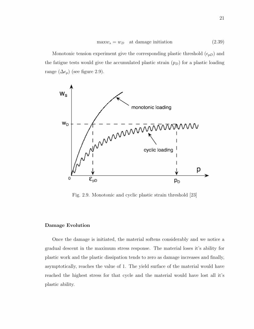
maxws = wD at damage initiation (2.39)
Monotonic tension experiment give the corresponding plastic threshold (εpD) and
the fatigue tests would give the accumulated plastic strain (pD) for a plastic loading
range (∆εp) (see figure 2.9).
Fig. 2.9. Monotonic and cyclic plastic strain threshold [23]
Damage Evolution
Once the damage is initiated, the material softens considerably and we notice a
gradual descent in the maximum stress response. The material loses it’s ability for
plastic work and the plastic dissipation tends to zero as damage increases and finally,
asymptotically, reaches the value of 1. The yield surface of the material would have
reached the highest stress for that cycle and the material would have lost all it’s
plastic ability.

22
2.2.4 Implementation of the Constitutive Model in FE Tool
There are many commercial FEA tools that enable us to model damage for mono-
tonic load cases. In the current research a commercial software that has incorporated
the damage model for cyclic loading with the help of direct cyclic algorithm (see
section 2.3), is used.
The step-wise procedure is as follows,
• Step 1: Get the cyclic stress-strain graph from stabilized cycles. Fit the curve so
that we obtain the parameters for combined hardening model.Use the parameter
for material input. These are critical to assess the hysteresis energy for damage
models.
• Step 2: Obtain cycles to damage initiation from cyclic stress-strain data and
calibrate it for the damage model.
• Step 3: Obtain fatigue life through experiment and calibrate the total life for
the damage evolution.
• Step 4: Use the model to predict fatigue life of material.
Many finite element tools support the combined hardening model and this could
be obtained under the plasticity section. To use the damage capability for fatigue,
the damage inititation and evolution critieria is defined using the hysteresis energy
option. In this existing finite element tool, this is achieved by adding the following
lines to the input file,
*Damage Initiation, criterion=HYSTERESIS ENERGY
Data1,Data2
*Damage Evolution, type=HYSTERESIS ENERGY
Data1,Data2
In the finite element tools, the damage initiation criteria is defined as the point
where the hysteresis energy reaches a certain threshold value leveraging the thermo-
23
dynamic theory. It assigns a cycles to initiation value that needs to be calibrated
(see [23] section 1.3 for more detail). The equation that finite element tools solves is,
N0 = C1∆WC2 (2.40)
where C1 and C2 are material properties that need to be calibrated. When number
of cycles N > N0, damage is initiated.
Once the damage is initiated, the material softens considerably and we notice a
gradual descent in the maximum stress response. The material loses it’s ability for
plastic work and the plastic dissipation tends to zero as damage increases and finally
asymptotically reaches it’s maximum value. The yield surface of the material would
have reached the highest stress for that cycle and the material would have lost all it’s
plastic ability.
The rate of loss of inelastic hysteresis energy is modelled to predict the fatigue
life of the material. Finite element tools have an established methodology for fatigue
where the damage would tend towards the value of 1 as the inelastic hysteresis energy
would tend towards zero and is given by,
dD
dN=C3
Le∆WC4 (2.41)
where, C3 and C4 are material properties that need to be calibrated, Le is the char-
acteristic length of the element. The characteristic length and it’s effects would be
discussed in the section 2.3.3.
Once this cycle number is reached, the damage manifests as macroscopic crack
and thus we would define that as the fatigue life for the material.

24
2.2.5 Procedure for Determination of Material Parameters
Cyclic Hardening Parameters
As seen in the previous section, for us to assess the fatigue life of material through
energy methods, the inelastic hysteresis energy should be accurately modelled. And
for that, the stress-strain curve should be captured in detail for cyclic loading. We are
using the combined hardening model, see eq.2.15, with four backstresses to simulate
the cyclic behavior. Now, the kinematic hardening parameters are derived from the
stress-strain data by the method of power law regression analysis [26]. Ideally, the
values of Ci and γi should be calibrated using both monotonic and cyclic data from
stabilized cycle.
The extraction of parameter is done through a optimization procedure through
MS Excel. A seed value of parameters Ci and γi is considered and then the value
of σ(p) is calculated using the equation 2.14. The difference in the calculated value
(from the seed values of Ci and γi) to the actual value through experiment (error) is
squared and added.
The objective is thus to minimize this error. Excel offers multiple tools to conduct
optimization studies. For our purposes we used the GRG non-linear solver with the
central difference method. The parameters thus calibrated are seen in Chapter 4.
Let the vector ~W be the calculated values from seed values and let ~V be the actual
value from the experiments, then objective function would be,
minimizen∑i=1
(Wi − Vi)(Wi − Vi) (2.42)
Damage Initiation Parameters
The cycles to damage initiation requires us to carefully plot the cyclic variation of
stress-strain hysteresis loops and observe when the angle of linear region (i.e, elastic
region) changes. We have defined damage such that E = E/(1 − D) and thus we

25
see a deterioration in the value of Young’s modulus, E, when damage is non-zero.
Loading the specimen cyclically between different strain ranges would give different
stable inelastic energy values and different cycle life. A plot of different inelastic
hysteresis energy values against cycles to damage initiation is created and a power
law regression is used to fit the model to the equation N0 = C1∆WC2 .
Fig. 2.10. Calculating damage initiation parameters C1 and C2 fromhysteresis energy [27]
Biglari et al. [27], conducted fatigue inspection for 9Cr steel at 620◦C. They
calibrated the damage initiation parameters by tabulating the variation of hysteresis
energy with cycles to damage initiation. The data is represented in figure 2.10. They
calibrated the initiation parameters to be C1 = 14.3 and C2 = −1.9.
Damage Evolution Parameters
The evolution of material degradation is calibrated by fitting the model for change
in inelastic hysteresis energy at different cycles. The experimental data is used to

26
calibrate dD/dN incrementally. Biglari et al. [27] conducted this calibration for
9Cr steel at 620◦C using figure 2.11. He obtained the value of C3 = 4X10⁻⁴ and
C4 = 0.91. The value of C3 is calibrated keeping the characteristic length of mesh
used.
Fig. 2.11. Calculating damage evolution parameters C3 and C4 [27]
2.3 Direct Cyclic Method
2.3.1 Need for a Quasi-static Approach
There are various ways to calculate the fatigue life of a component. The most
popular way is to conduct a static analysis on the component and after looking up
the regions of stress and it’s distribution, compare the values to a standard Stress-life
curve. These charts provide the life of a component against a given stress value. For
low cycle fatigue, a similar strain-life curve is used to assess the life of the material
more popularly. The strain measure is accurate for low cycle fatigue regimes. Another
way is to refer the Coffin Manson laws to predict the life for both HCF and LCF. These

27
too would require static analysis result and assume that the rate of crack propagation
is linear. Also, we intended to capture the effect of damage through cycles.
To achieve that would be computationally prohibitive. The fatigue analysis in-
volves repeated cycles of static loading and to run those many static cycles is ineffi-
cient. Even to predict the stable hysteresis loop for a material subjected to reversed
plastic strain cycles would require considerable computation time.
Direct methods for finding stabilized material response were explored for the very
same reason. The methodology incorporated in commercial finite element tools is
based on the seminal works of Dang and Maitournam [28] who leveraged the cyclic
behavior to find Fourier series expansion. The overall methodology is shown in figure
2.12.
Fig. 2.12. Methodology incorporated by Dang et al. [28]

28
The stable cycles which are predicted by the hardening laws are reached by enforc-
ing the deformation and force ranges to acquire cyclic values consistent with values at
the stabilized cycle. This method predicts the asymptotic material response directly
without actually calculating through all cycles. The method works on large time
incrementation method and seeks the mechanical fields which have the same values
at the end of a loading cycle as the beginning of the cycle. This method can predict
elastic and plastic shakedown as well as ratchetting [28].
2.3.2 Implementation in FE Model
We can incorporate direct cyclic algorithm using user defined subroutines. Few
commercial finite element tools incorporate the direct cyclic algorithm for both ar-
riving at the aymptotic response as well as predicting the fatigue life. The program
solves the familiar equilibrium equation using Newton’s method, but the equilibrium
equations are now cyclic in nature such that,
R(t) = F (t)− I(t) = 0 (2.43)
where, F (t) is the descretized form of cyclic load such that F (t+T ) = F (t) with time
period T , I(t) is the internal force vector and R(t) is the residual vector.
As discussed earlier, we need a displacement definition that is uqual to the values
at asymptotic cycle state and thus [29],
u(t) = u0 +n∑k=1
[usk sin kωt+ uck cos kωt (2.44)
where n is the number of Fourier terms used, ω is the angular frequency, and u0, usk, u
ck
are unknown displacement co-efficients. The equilibrium equations representing the
process are then written as,
Kci+1k = Ri
k (2.45)

29
where, k is the elastic stiffness matrix and i is the iteration number. The residual
vector is similarly expanded as the displacement function [29],
R(t) = R0
n∑k=1
[Rsk sin kωt+Rc
k cos kωt] (2.46)
where the R0, Rsk, R
ck are found by the fourier term expansion.
Fig. 2.13. Comparison of stabilized cycle obtained by direct methodwith static cycling method
The difference between the input and response is fed back as corrections to find
the stabilized cycle. The figure 2.13 shows the stabilized state achieved with direct
cyclic algorithm with the material loaded cycle by cycle. The computation time saved
was significant.
2.3.3 Solution Accuracy
The implementation of fatigue analysis with direct cyclic method needs hysteresis
energy for damage calculations. But it is to be noted that the hysteresis energy is
sensitive to mesh parameter with it reaches large values as mesh size decreases [30].

30
Fig. 2.14. Convergence study for damage parameter
To alleviate this issue, characteristic length is introduced in the damage evolution
equation 2.41. According to reference [31],
The characteristic length is based on the element geometry and formu-
lation: it is a typical length of a line across an element for a first-order
element; it is half of the same typical length for a second-order element.
For beams and trusses it is a characteristic length along the element axis.
For membranes and shells it is a characteristic length in the reference
surface. For axisymmetric elements it is a characteristic length in the rz
plane only. For cohesive elements it is equal to the constitutive thickness.
This definition of the characteristic length is used because the direction
in which fracture occurs is not known in advance. Therefore, elements
with large aspect ratios will have rather different behavior depending on
the direction in which the damage occurs: some mesh sensitivity remains
because of this effect, and elements that are as close to square as possible

31
are recommended. However, since the damage evolution law is energy
based, mesh dependency of the results may be alleviated [31].
Therefore, a mesh convergence study targeting the characteristic length has to be
conducted as shown in figure 2.14. The characteristic lengths used in this report are
0.266 for the axisymmetric element and 1.58 for the solid brick element.

32
3. EXPERIMENTAL PROCEDURE
3.1 Preparation of Specimen
The 3D printed specimen is printed using a powder bed fusion process using EOS
270 M. The powder is obtained from EOS who specialise in manufacturing metal
powder for 3D printing application. The PH1 series of steels are pre-alloyed steels
characterized by good corrosion resistance and excellent mechanical properties [32].
The chemical composition is as shown in table 3.1,
Table 3.1.Chemical composition of 3D printed 15-5 PH stainless steel [32].
Element % by Weight
Carbon 0.07
Manganese 1.00
Silicon 1.00
Chromium 14.00-15.50
Nickel 3.50-5.50
Copper 2.50-4.50
Molybdenum 0.50
Niobium 0.15-0.45
Iron Balance
The figure 3.1 shows the SEM image of the powder used to print the specimen for
the fatigue test. The average size of the particle can be seen as around 20 µm.
The printed specimen, see figure 3.2 is as per the specification for the the fatigue
tester by TERCO for their fatigue testing machine MT3120 [33]. Originally the

33
specimen was printed with support structures which need to be machined off before
using them in the fatigue tester. This was achieved by initially using hack saw blade
to remove a considerable portion of support before using a grinding machine to give
an accurate finish.
Fig. 3.1. SEM image of 15-5 PH powder [34]
Fig. 3.2. 15-5 PH rotating bending specimen

34
3.2 Fatigue Testing of Specimen
The fatigue testing machine used was MT3120 fatigue tester from TERCO sweden.
The working principle for the machine is as shown in figure 3.3. The actual tester is
shown in figure 3.4.
Fig. 3.3. Functioning of MT3120 [33]
Fig. 3.4. MT3210 Fatigue tester [33]

35
The specimen showed previously is loaded at the free end in the fatigue tester.
The tester has a digital cycle counting device that keeps track of the loading cycles
and it automatically stops on specimen failure. The 3D printed specimen were loaded
for 3 different strain ranges and the cycles to failure was noted.
3.3 Results and Discussion
The results of the fatigue test is tabulated below,
Table 3.2.Fatigue result tabulation
% strain amplitude εa No. of reversals to failure
0.132 46760
0.189 33183
0.214 13403
Fig. 3.5. Result of the fatigue test
36
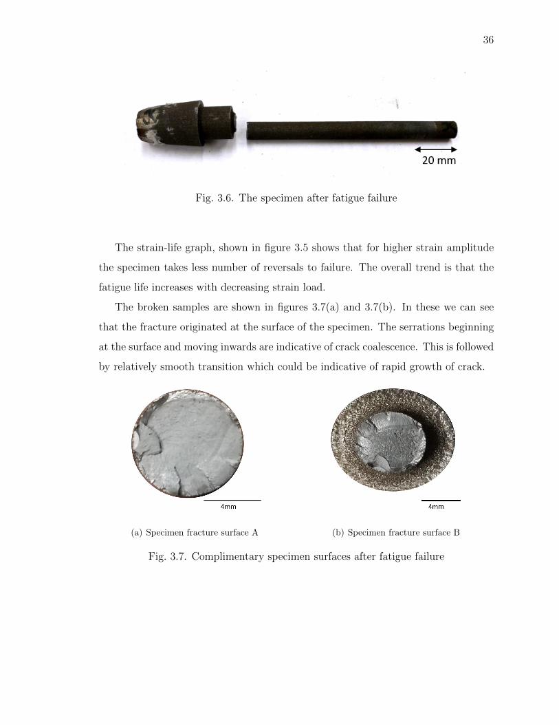
Fig. 3.6. The specimen after fatigue failure
The strain-life graph, shown in figure 3.5 shows that for higher strain amplitude
the specimen takes less number of reversals to failure. The overall trend is that the
fatigue life increases with decreasing strain load.
The broken samples are shown in figures 3.7(a) and 3.7(b). In these we can see
that the fracture originated at the surface of the specimen. The serrations beginning
at the surface and moving inwards are indicative of crack coalescence. This is followed
by relatively smooth transition which could be indicative of rapid growth of crack.
(a) Specimen fracture surface A (b) Specimen fracture surface B
Fig. 3.7. Complimentary specimen surfaces after fatigue failure

37
4. NUMERICAL MODELLING
Two calibration tests have been simulated using finite element method to demonstrate
viability of the model. This is followed by two prediction simulations for 15-5 PH
stainless steel. In these simulations, the fatigue prediction is made utilising the direct
cyclic algorithm and the cyclic behavior during multiple amplitude strain loading
is simulated using the static analysis method. This is because, as mentioned in
the section 2.3, the direct cyclic method converges only to the asymptotic stress-
strain cycle and thus wouldn’t capture the intermediate effect of cyclic hardening or
softening. To see how the material behaves through cycles, initially static analysis
method is considered.
4.1 Model Validation
4.1.1 CASE 1: Fatigue Prediction for 3D Printed 17-4 Stainless Steel
under Constant Amplitude Strain Load: Direct Cyclic Method
The test is to accurately capture the fatigue life of 3D printed 17-4 stainless steel
as mentioned in Yadollahi et al. [6]. This specimen was vertically printed. The paper
provides the cyclic stress-strain variation and fatigue life at different strain ampli-
tudes. Using these data, the non-linear kinematic hardening parameters, damage
initiation and damage evolution parameters were independently calibrated.
Geometry, Mesh and Boundary Condition
The geometry is that of a standard tension compression fatigue test specimen.
The specimen is modelled using axisymmetric elements with 1700 elements and
1806 nodes. The associated characteristic length is 0.266. The element type is ca-

38
(a) Mesh (b) Boundary condition
Fig. 4.1. FE model for axial Tension-compression fatigue test specimen
Fig. 4.2. Load function

39
pable of modelling non-linear plasticity. The model was also symmetrical about the
plane perpendicular to it’s long axis as shown in figure 4.1. This was done to save
computational time and effort.
The specimen was loaded cyclically at top using a cyclic displacement function.
The tests were conducted for three strain ranges all multiplied by the amplitude of
the displacement function. The three strain ranges were 0.3%, 0.4%, and 0.5%.
Material Parameters
The Young’s modulus of the vertically printed, as-built 17-4 PH stainless steel is
187.3 GPa and it’s yield strength is given as 580 MPa. The cyclic material parameters
were curve fitted using the data given in Yadollahi et al. [6] for the vertically printed,
as built specimen. Their cyclic hardening model obtained from stabilized cycle was
modified to accommodate the combined hardening model with three backstresses
using equation 2.15.
Fig. 4.3. Material characterization for 17-4 [6]

40
Fig. 4.4. Regression fit for damage evolution
Table 4.1.Backstresses Ci and γi values for 3D printed 17-4 stainless steel
Backstresses Ci (MPa) γi
1 1.83e+5 104516
2 7.145e+4 676060.6
3 7.39e+4 142.59
Table 4.2.Damage parameters for 3D printed 17-4 stainless steel
Damage parameters Values
C1 14.3 [27]
C2 -0.91 [27]
C3 1e-4
C4 1.024

41
The damage parameters were calibrated based on the fatigue life at defined strain
amplitudes per Yadollahi [6]. The data provided cannot be used to calibrate damage
initiation parameter and thus a nominal value obtained from Bilgari et al. [27] is used
in this simulation. The damage evolution parameters are fit for three different strain
ranges giving three different hysteresis energy curves, see figure 4.4.
Since our characteristic length is 0.266, we will get the damage evolution param-
eters as shown in table 4.2.
4.1.2 CASE 2: Cyclic Behavior Simulation for Alloy 617 under Multi-
amplitude Strain Load: Static Analysis Method
Pritchard [35] conducted experiments detailing the behavior of steel Alloy 617.
The focus of his work was to establish fatigue life and fatigue-creep life of the alloy
and explored strain rate dependence of material parameters. An attempt has been
made to replicate the the multi-amplitude strain range behavior.
Fig. 4.5. Multi-amplitude strain
42
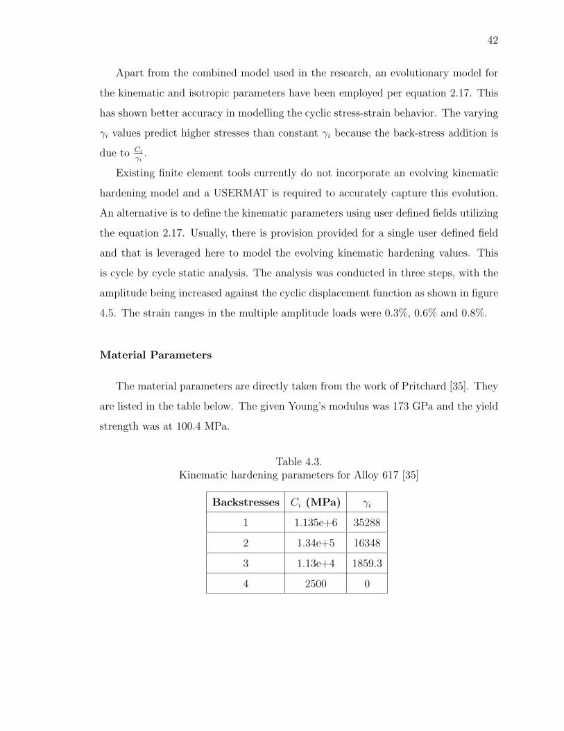
Apart from the combined model used in the research, an evolutionary model for
the kinematic and isotropic parameters have been employed per equation 2.17. This
has shown better accuracy in modelling the cyclic stress-strain behavior. The varying
γi values predict higher stresses than constant γi because the back-stress addition is
due to Ci
γi.
Existing finite element tools currently do not incorporate an evolving kinematic
hardening model and a USERMAT is required to accurately capture this evolution.
An alternative is to define the kinematic parameters using user defined fields utilizing
the equation 2.17. Usually, there is provision provided for a single user defined field
and that is leveraged here to model the evolving kinematic hardening values. This
is cycle by cycle static analysis. The analysis was conducted in three steps, with the
amplitude being increased against the cyclic displacement function as shown in figure
4.5. The strain ranges in the multiple amplitude loads were 0.3%, 0.6% and 0.8%.
Material Parameters
The material parameters are directly taken from the work of Pritchard [35]. They
are listed in the table below. The given Young’s modulus was 173 GPa and the yield
strength was at 100.4 MPa.
Table 4.3.Kinematic hardening parameters for Alloy 617 [35]
Backstresses Ci (MPa) γi
1 1.135e+6 35288
2 1.34e+5 16348
3 1.13e+4 1859.3
4 2500 0

43
Table 4.4.Isotropic hardening parameters for Alloy 617 [35]
Q∞ MPa b
37.61 61.33
Table 4.5.Kinematic hardening evolution parameters [35]
No. Li di
1 -12800 7.496
2 -4875.7 10.07
3 -634.4 18.57
4 0 1
4.2 Simulations of 3D Printed 15-5 PH Stainless Steel
4.2.1 CASE 3: Fatigue Prediction under Constant Amplitude Strain
Load: Direct Cyclic Method
The fatigue analysis is carried out using the direct cyclic approach. Stable cycles
are reached and, damage initiation and accumulation parameters modify the structure
response. The simulation is conducted for three different constant strain amplitude.
Geometry, Mesh and Boundary Condition
The geometry is modeled as standard test specimen for rotating bending fatigue
tests presented in Chapter 3. The simple geometry was created using a CAD modeler.
The radius of the bending specimen is 4 mm and length is 100 mm per standard
specimen. 8 noded Brick elements with reduced integration formulation (C3D8R) are
used in this simulation. There are 3792 elements and 4523 nodes. The characteristic
length of the elements is 1.58. The elements are created with a bias such that there are

44
(a) Mesh (b) Boundary condition
Fig. 4.6. FE model for the rotary fatigue specimen
more elements near the fixed point of the cantilever beam as opposed to the free end.
The model is constrained at one end and is free to move at the other. A displacement
boundary condition is applied to the free end. See figure 4.6(a) and 4.6(b).
The same displacement function shown in 4.2 was used to apply strain loads. The
analysis was conducted for three total strain ranges of 1.87%, 1.58% and 1.37%.
Material Parameters
The non-linear hardening models parameters are fit for 4 backstresses from the
data of the monotonic stress-strain graph from 4.7. As mentioned before, ideally the
fit should be made using both monotonic and cyclic curves. But given the current
set of data, we can predict how the material will behave under cyclic loads.

45
From the stress-strain data it was ascertained that the Young’s modulus was 78.85
GPa and yield limit of the specimen was 820 MPa and thus the plastic strain data
was captured. The entirety of the data was sampled at an interval of 100 to reduce
the data to manageable portion. The Ci and γi are listed in the table 4.6, and a curve
representing total backstress and it’s relation to it’s additive components is shown in
figure 4.9. The parameter values were obtained by the curve fit (see figure 4.8).
Fig. 4.7. Experimentally measured uniaxial tension Stress-straingraph for 3D printed 15-5 PH stainless steel
Table 4.6.Backstresses Ci and γi values for 3D printed 15-5 PH stainless steel
Backstresses Ci (MPa) γi
1 3.45e+05 23435.577
2 1.44e+05 108732.63
3 2.88e+04 14737.23
4 3.71e+03 37.055

46
Fig. 4.8. Curve fit applied to experimental data
Fig. 4.9. Total backstress(solid line) and it’s decomposed components
47
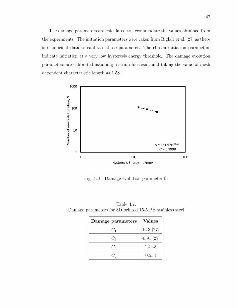
The damage parameters are calculated to accommodate the values obtained from
the experiments. The initiation parameters were taken from Biglari et al. [27] as there
is insufficient data to calibrate those parameter. The chosen initiation parameters
indicate initiation at a very low hysteresis energy threshold. The damage evolution
parameters are calibrated assuming a strain life result and taking the value of mesh
dependent characteristic length as 1.58.
Fig. 4.10. Damage evolution parameter fit
Table 4.7.Damage parameters for 3D printed 15-5 PH stainless steel
Damage parameters Values
C1 14.3 [27]
C2 -0.91 [27]
C3 1.4e-3
C4 0.553

48
4.2.2 CASE 4: Cyclic Behavior Simulation under Multi-amplitude Strain
Load: Static Analysis Method
The simulation undertaken in section 4.1.2 is repeated for the case of 15-5 PH
stainless steel. The axisymmetric geometry, mesh and boundary condition is similar
to the ones used in the mentioned section. The Young’s modulus and yield strength
for 15-5 PH stainless steel from the stress-strain data is used (see section 4.2) and
kinematic hardening material property used is the same as in table 4.6. In this case,
the kinematic hardening evolution parameters are included.
The kinematic hardening evolution parameters are take from the reference used
in section 4.1.2 in table 4.5 [6]. The procedure remains similar to section 4.1.2. Only
the displacement amplitudes are changed for this simulation as seen in figure 4.11.
The displacement amplitudes are different because, 15-5 PH stainless steel yields at
a much higher strain than Alloy 617 used in section 4.1.2.The multi-amplitude strain
range has the split 1.15%, 1.6% and 1.75%.
Fig. 4.11. Multi-amplitude strain for CASE 4
49
4.3 Results and Discussion
4.3.1 CASE 1: Fatigue Prediction for 3D Printed 17-4 Stainless Steel
under Constant Amplitude Strain Load
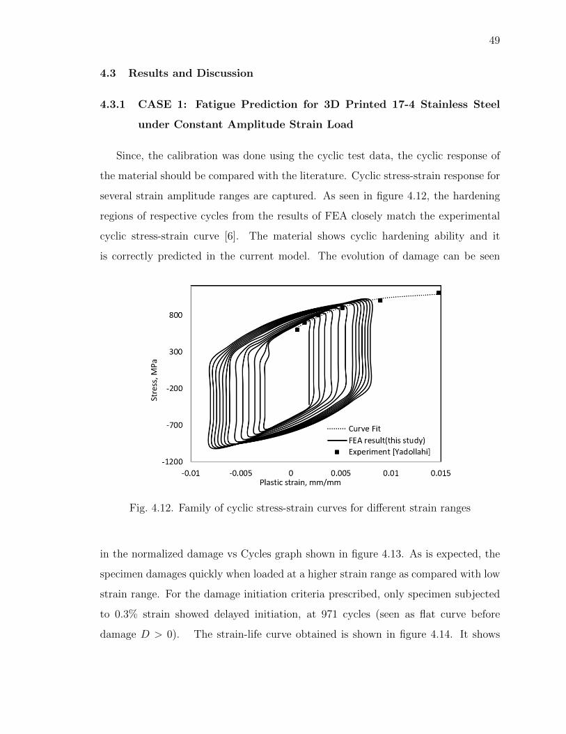
Since, the calibration was done using the cyclic test data, the cyclic response of
the material should be compared with the literature. Cyclic stress-strain response for
several strain amplitude ranges are captured. As seen in figure 4.12, the hardening
regions of respective cycles from the results of FEA closely match the experimental
cyclic stress-strain curve [6]. The material shows cyclic hardening ability and it
is correctly predicted in the current model. The evolution of damage can be seen
Fig. 4.12. Family of cyclic stress-strain curves for different strain ranges
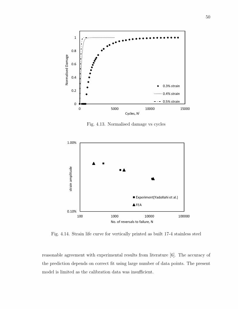
in the normalized damage vs Cycles graph shown in figure 4.13. As is expected, the
specimen damages quickly when loaded at a higher strain range as compared with low
strain range. For the damage initiation criteria prescribed, only specimen subjected
to 0.3% strain showed delayed initiation, at 971 cycles (seen as flat curve before
damage D > 0). The strain-life curve obtained is shown in figure 4.14. It shows
50
Fig. 4.13. Normalised damage vs cycles
Fig. 4.14. Strain life curve for vertically printed as built 17-4 stainless steel
reasonable agreement with experimental results from literature [6]. The accuracy of
the prediction depends on correct fit using large number of data points. The present
model is limited as the calibration data was insufficient.

51
4.3.2 CASE 2: Cyclic Behavior Simulation for Alloy 617 under Multi-
amplitude Strain Load
The modified parameters were a reasonable approximation as it captured the
intended effect on stress evolution. As discussed earlier, the introduction of the
kinematic hardening evolution parameter ensures that higher stresses are predicted
for the same plastic strain regime since the given values of Li and di cause the γi
value to decrease, which in turn causes the backstress values to increase. Figure 4.15
shows this comparison of the results obtained using modified parameters in FEA and
the results from literature.
Fig. 4.15. Comparison of FEA result with literature [35]
The variation of the stress-strain curves are shown for different cycles in the figure
4.16. This figures captures the effect of combined hardening model used. We can see
that the hysteresis loops shift upwards for higher cycles within a strain range. The
kinematic evolution parameters indicate an increased number of cycles to a stabilized
regime. As, the load is increased, the material would resist hardening (stress response
will plateau) and damage would initiate. After this, the material would soften..

52
Fig. 4.16. Variation of stress-strain loops for different strain range
4.3.3 CASE 3: Fatigue Prediction for 3D printed 15-5 PH Stainless Steel
under Constant Amplitude Strain Load
The progression of damage parameter as cycles progress for different strain ranges
are shown in figure 4.17. Since the damage initiation parameters are nominal, damage
would begin for minimal hysteresis energy, which is achieved at all strain amplitude
ranges in our simulations.
The rate of energy dissipation, and thus that of damage evolution, would be
highest for the highest strain amplitude range and this is seen in the figure. The
damage parameter has a power law relationship with cycles and thus is non-linear.
The calibration of damage evolution of damage parameters shows good agreement
with values used to calibrate (see figure 4.18). The predicted strain life from finite
element model and the calibration life values are close to each other with higher
strains resulting in shorter life. The results would be more accurate with large data
points as it would smooth-en the curve out.

53
Fig. 4.17. Variation of damage parameter with cycles for different strain ranges
Fig. 4.18. Comparison of strain life curve between fit data and FEA

54
The model is extended (see figure 4.19) to cover the lower strain regions that
the experiment covered. The Coffin-Manson-Basquin combined law is fit and the
predicted curve passes close to the experimental values. The Coffin-Manson-Basquin
parameters referring equation 2.4 is given in table 4.8.
Table 4.8.Coffin-Mason-Basquin parameters for 3D printed 15-5 PH stainless steel
Parameters Values
σ′
f GPa 70.92
b -0.7455
ε′
f 9.884
c -0.405
Fig. 4.19. Comparison between experimental data and Coffin-Manson-Basquin prediction for 3D printed 15-5 PH stainless steel
The variation of stress for the strain amplitude loading of 1.87% can be seen from
figure 4.20. As, in our simulation, damage starts at the first cycle, the material softens
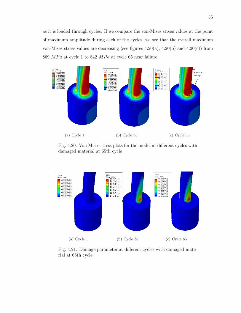
55
as it is loaded through cycles. If we compare the von-Mises stress values at the point
of maximum amplitude during each of the cycles, we see that the overall maximum
von-Mises stress values are decreasing (see figures 4.20(a), 4.20(b) and 4.20(c)) from
869 MPa at cycle 1 to 842 MPa at cycle 65 near failure.
(a) Cycle 1 (b) Cycle 35 (c) Cycle 65
Fig. 4.20. Von Mises stress plots for the model at different cycles withdamaged material at 65th cycle
(a) Cycle 1 (b) Cycle 35 (c) Cycle 65
Fig. 4.21. Damage parameter at different cycles with damaged mate-rial at 65th cycle

56
The corresponding damage parameter plot at different cycles are plotted in figure
4.21. On the first cycle we see that the damage has not initiated yet, because, as
per our criterion, damage initiation is after the first cycle. The damage progresses as
the specimen is cycled through constant amplitude strain and reaches it’s maximum
value at cycle 65 for failure. At this stage, the material has lost it’s capacity for
plastic work.
4.3.4 CASE 4: Cyclic Behavior Simulation for 3D Printed 15-5 PH Stain-
less Steel under Multi-amplitude Strain Load
Fig. 4.22. Cycle dependent stress variation
The kinematic hardening evolution parameters used in this model increased the
backstress component during stress-strain reversals. As is seen in figure 4.22 the
predicted values of stresses are higher when hardening evolution model is used. Since,
these values are borrowed from literature, the actual stress evolution behavior needs
to be tracked and then the γi evolution needs to be calibrated to new Li and di values
to accurately capture the behavior.

57
Fig. 4.23. Stress-strain curve
The stress-strain graph is shown in figure 4.23 associated with the hardening
evolution model. The yield limit of 15-5 PH stainless steel is several times higher
than the values used for Alloy 617 and the hysteresis curve would be narrower. This
could indicate a more brittle interaction as compared to Alloy 617.

58
5. CONCLUSION
In this thesis, a combined numerical and experimental study is presented. The major
conclusions are summarized as follows.
• The fatigue life of the 15-5 PH stainless steel is experimentally measured. The
strain life curve shows that the numbers of the reversals to failure increase from
13,403 to 46,760 as the applied strain magnitudes decrease from 0.214% from
0.132%, respectively. The microstructure analysis shows that predominantly
brittle fracture is presented on the fractured surface
• A finite element model based on cyclic plasticity including the damage model
is developed to predict the fatigue life. The model is calibrated with two cases:
one is the fatigue life of 3D printed 17-4 stainless steel under constant amplitude
strain load using the direct cyclic method, and the other one is the cyclic be-
havior of Alloy 617 under multi-amplitude strain loads using the static analysis
method. Both validation models show a good correlation with the literature
experimental data
• After the validation, the finite element model is applied to the 15-5 PH stainless
steel. Using the direct cyclic method, the model predicts the fatigue life of 15-5
PH stainless steel under constant amplitude strain. The extension of the pre-
diction curve matches well with the previously measured experimental results,
following the Coffin-Manson-Basquin Law. Under multi-amplitude strain, the
kinematic hardening evolution parameter is incorporated into the model. Higher
stresses are predicted when strain amplitudes are increased
• The model presented in the work can be used to design for the reliability of 3D
printed metals under cyclic loading conditions.

59
6. RECOMMENDATIONS
The current model can be further implemented as follows,
• Conduct fatigue tests at low-cycle conditions to better compare against model-
ing data.
• The strain controlled cyclic tests need to be conducted for 15-5 PH stainless
steel to find the cycles to stabilization, cycles to damage initiation and the
rate of decrease of the materials ability to do plastic work. This would help
characterize the material behavior with greater accuracy.
• These cyclic tests should be conducted for different strain rates and an under-
standing of strain rate dependence on the fatigue life needs to be assessed.
• The cyclic tests can also incorporate temperature dependency and understand
the effects on cyclic behavior.
• For components produced by different 3D printing process, the relationship
between 3D printing parameters and the parameters in the model need to be
determined.
• This model should be used to predict the fatigue life for different design pa-
rameters under complex loading conditions. This knowledge can then guide the
design intent.
• The model can be extended to incorporate the effect of creep.

REFERENCES

60
REFERENCES
[1] P. Paris, M. Gomez, and W. Anderson, “A rational analytical theory of fatiguethe trend in engineering,” U. of Washington, Seattle, Wa, vol. 13, no. 1, 1961.
[2] J. Sehrt and G. Witt, “Dynamic strength and fracture toughness analysis of beammelted parts,” in Proceedings of the 36th international MATADOR conference.Springer, 2010, pp. 385–388.
[3] A. B. Spierings and G. Levy, “Comparison of density of stainless steel 316l partsproduced with selective laser melting using different powder grades,” in Proceed-ings of the Annual International Solid Freeform Fabrication Symposium. Austin,TX, 2009, pp. 342–353.
[4] T. L. Starr and A. Spierings, “Tensile and fatigue performance of laser sinteredstainless steels,” in Proceedings of the Annual International Solid Freeform Fab-rication Symposium, Austin, Texas. HW-Verlag, 2010.
[5] A. B. Spierings, N. Herres, and G. Levy, “Influence of the particle size distri-bution on surface quality and mechanical properties in am steel parts,” RapidPrototyping Journal, vol. 17, no. 3, pp. 195–202, 2011.
[6] A. Yadollahi, N. Shamsaei, S. M. Thompson, A. Elwany, and L. Bian, “Effectsof building orientation and heat treatment on fatigue behavior of selective lasermelted 17-4 ph stainless steel,” International Journal of Fatigue, vol. 94, pp.218–235, 2017.
[7] R. Branco, J. Costa, F. Berto, S. Razavi, J. Ferreira, C. Capela, L. Santos, andF. Antunes, “Low-cycle fatigue behaviour of aisi 18ni300 maraging steel producedby selective laser melting,” Metals, vol. 8, no. 1, p. 32, 2018.
[8] L. Toth and S. Y. Yarema, “Formation of the science of fatigue of metals. part1. 1825–1870,” Materials Science, vol. 42, no. 5, pp. 673–680, 2006.
[9] R. Smith, “The versailles railway accident of 1842 and the first research intometal fatigue.(retroactive coverage),” Fatigue 90, pp. 2033–2041, 1990.
[10] O. Basquin, “The exponential law of endurance tests,” in Proc Am Soc TestMater, vol. 10, 1910, pp. 625–630.
[11] A. Milton, “Miner: Cumulative damage in fatigue journal of appl,” Mech, 1945.
[12] L. Coffin, “The cyclic straining and fatigue of metals,” Trans Metall Soc AIME,vol. 215, p. 794, 1959.
[13] S. Manson and M. Hirschberg, “Fatigue: an interdisciplinary approach,” Syra-cuse University Press, Syracuse, NY, p. 133, 1964.

61
[14] S. Manson, “Fatigue: a complex subjectsome simple approximations,” Experi-mental mechanics, vol. 5, no. 7, pp. 193–226, 1965.
[15] W. Cui, “A state-of-the-art review on fatigue life prediction methods for metalstructures,” Journal of marine science and technology, vol. 7, no. 1, pp. 43–56,2002.
[16] W. R. Osgood, “Stress-strain formulas,” Journal of the Aeronautical Sciences,vol. 13, no. 1, pp. 45–48, 1946.
[17] R. Hill, The mathematical theory of plasticity. Oxford university press, 1998,vol. 11.
[18] J.-L. Chaboche, “A review of some plasticity and viscoplasticity constitutivetheories,” International journal of plasticity, vol. 24, no. 10, pp. 1642–1693, 2008.
[19] J. Bauschinger, “On the changes of the elastic limit and the strength of iron andsteel by straining in tension and compression, by heating and by cooling and byfrequently repeated loading,” Mitt Mech, vol. 13, no. 3, pp. 1–115, 1886.
[20] J. Bree, “Elastic-plastic behaviour of thin tubes subjected to internal pressureand intermittent high-heat fluxes with application to fast-nuclear-reactor fuelelements,” Journal of strain analysis, vol. 2, no. 3, pp. 226–238, 1967.
[21] C. O. Frederick and P. Armstrong, “A mathematical representation of the mul-tiaxial bauschinger effect,” Materials at High Temperatures, vol. 24, no. 1, pp.1–26, 2007.
[22] S. Krishna, T. Hassan, I. B. Naceur, K. Saı, and G. Cailletaud, “Macro versusmicro-scale constitutive models in simulating proportional and nonproportionalcyclic and ratcheting responses of stainless steel 304,” International Journal ofPlasticity, vol. 25, no. 10, pp. 1910–1949, 2009.
[23] J. Lemaitre, A Course on Damage Mechanics, 2nd ed. Springer Science BusinessMedia, 1996.
[24] L. Kachanov, Introduction to continuum damage mechanics. Springer Science& Business Media, 2013, vol. 10.
[25] Y. N. Rabotnov, Creep problems in structural members. North-Holland Seriesin Applied Mathematics and Mechanics, 1969, vol. 7.
[26] D. Dewees, “Ratcheting and cyclic plasticity considerations for code analysis,”(Retrieved 06-May-2019). [Online]. Available: https://www.efatigue.com/training/Chapter 5.pdf
[27] F. Biglari, P. Lombardi, S. Budano, C. Davies, and K. Nikbin, “Predicting dam-age and failure under low cycle fatigue in a 9cr steel,” Fatigue & Fracture ofEngineering Materials & Structures, vol. 35, no. 12, pp. 1079–1087, 2012.
[28] K. D. Van and M. H. Maitournam, “On a new methodology for quantitative mod-eling of fretting fatigue,” in Fretting fatigue: current technology and practices.ASTM International, 2000.

62
[29] “Abaqus user manual V6.14,” (Retrieved 01-May-2019). [Online].Available: https://abaqus-docs.mit.edu/2017/English/SIMACAETHERefMap/simathe-c-directcyclic.htm
[30] Z. P. Bazant and J. Ozbolt, “Nonlocal microplane model for fracture, damage,and size effect in structures,” Journal of Engineering Mechanics, vol. 116, no. 11,pp. 2485–2505, 1990.
[31] “Abaqus user manual V6.14,” (Retrieved 01-May-2019). [Online].Available: https://abaqus-docs.mit.edu/2017/English/SIMACAEANLRefMap/simaanl-c-directcyclicfatigue.htm
[32] “EOS stainless steel PH1 for EOSINT M 270,” (Retrieved 06-March-2018).[Online]. Available: http://gpiprototype.com/images/PDF/EOS-StainlessSteel-PH1.pdf
[33] “TERCO MT3012 fatigue tester,” (Retrieved 06-May-2018). [Online]. Avail-able: https://www.tercosweden.com/wp-content/uploads/2019/04/Material-Testing-Lab Lres.pdf
[34] S. Sagar, Y. Zhang, L. Wu, H.-Y. Park, J.-H. Lee, Y.-G. Jung, and J. Zhang,“Room-temperature charpy impact property of 3d-printed 15-5 stainless steel,”Journal of Materials Engineering and Performance, vol. 27, no. 1, pp. 52–56,2018.
[35] P. G. Pritchard, “High temperature fatigue and fatigue-creep responses of al-loy 617-experimental and unified constitutive modeling.” Master’s thesis, NorthCarolina State University, 2014.

VITA

63
VITA
List of Publications
Padmanabhan, A., & Zhang, J. (2018). Cybersecurity risks and mitigation strategies
in additive manufacturing. Progress in Additive Manufacturing, 3(1-2), 87-93.
List of Presentations
Padmanabhan, A., & Zhang, J.(2018, April). Fatigue characterization of 3D printed
15-5 stainless steel. Poster session presented at IUPUI Research Day, Indianapolis,
Indiana.
Padmanabhan, A., Sagar, S. & Zhang, J.(2018, June). Temperature-dependent Impact
Properties of 3D Printed 15-5 Stainless Steel . Poster session presented at POWDER-
MET2018 conference, San Antonio, Texas.
Padmanabhan, A., & Zhang, J.(2018, June). Fatigue characterization of 3D printed
15-5 stainless steel. Poster session presented at POWDERMET2018 conference, San
Antonio, Texas.
Padmanabhan, A., & Zhang, J.(2018, October). Analysis of fatigue behavior of 3D
printed 15-5 stainless steel - A combined modeling and experimental approach. Paper
presented at MS&T conference, Columbus, Ohio.
Awards
National science foundation(NSF) travel grant for POWDERMET2018.


![Early Corrosion Fatigue Damage on Stainless Steels Exposed ... · surrounding environment [13,14]. Then, corrosion fatigue is defined as a synergistic effect in which corrosion and](https://img.dokumen.tips/doc/110x75/6047f176e1f3ef03307425bb/early-corrosion-fatigue-damage-on-stainless-steels-exposed-surrounding-environment.jpg)