This document is downloaded from theVTT’s Research Information Portalhttps://cris.vtt.fi

VTThttp://www.vtt.fiP.O. box 1000FI-02044 VTTFinland

By using VTT’s Research Information Portal you are bound by thefollowing Terms & Conditions.

I have read and I understand the following statement:

This document is protected by copyright and other intellectualproperty rights, and duplication or sale of all or part of any of thisdocument is not permitted, except duplication for research use oreducational purposes in electronic or print form. You must obtainpermission for any other use. Electronic or print copies may not beoffered for sale.

VTT Technical Research Centre of Finland

Fatigue of stainless steel in NPP piping – challenges in design by analysisSolin, Jussi

Published in:Baltica XI

Published: 01/01/2019

Document VersionPublisher's final version

Link to publication

Please cite the original version:Solin, J. (2019). Fatigue of stainless steel in NPP piping – challenges in design by analysis. In Baltica XI:International Conference on Life Management and Maintenance for Power Plants VTT Technical ResearchCentre of Finland.

Download date: 14. Nov. 2021

Fatigue of stainless steel in NPP piping – challenges in design by analysis

Jussi Solin

VTT Technical Research Centre of Finland Ltd Espoo, Finland

Abstract

Design criteria set in the ASME Boiler and Pressure Vessel Code, Section III of 1963 have played a major role in designing and fatigue management of primary piping in nuclear power plants. Annealed austenitic stainless steel is widely used as pressure boundary against the hot coolant water, not only because of its corrosion resistance, but also because soft austenite is ductile and defect tolerant, i.e. difficult to break. Cyclic behaviour of stainless steels is complex and realistic fatigue assessment is challenging. Instead of preventing unexpected fracture, a more common concern seems to be tendency for overly conservatism, in particular after the change of stainless steel design curve in 2009. This paper revisits the background, evolution, unintentional changes and status of the design criteria. Revision of the design curve will be critically discussed, aiming to explain why the high cycle part of the new curve is questionable.

1. Introduction

This paper aims to discuss various challenges in applicability of the current fatigue design curves and rules for austenitic stainless steel in nuclear power plant (NPP) primary piping. My focus is in the ASME Boiler and Pressure Vessel Code section III, but the design philosophies and discussed issues are more or less common for all international design codes applied for unfired pressure equipment, e.g. ASME VIII (non-nuclear), RCC-M (French; applied also for OL3), KTA (German), and JSME (Japanese) [1–4]. Serious accidents in the past had shown deficiencies in designing safe pressure equipment for demanding and/or critical applications, such as the reactor pressure vessels (RPV) for NPP. A new era began, when The American Society for Mechanical Engineering (ASME) published their new code in 1963. ASME Sections III and VIII introduced a comprehensive approach for “design by analysis” with design curves based on strain controlled Low Cycle Fatigue (LCF) [5]. The primary aim was to prevent catastrophic fractures, fatigue and crack growth due to thermal transients in heavy section vessels experiencing limited numbers of thermal cycles, which cannot be limited in amplitude below the material endurance limit and exceed the allowable fatigue loading also in the High Cycle Fatigue (HCF) regime.

This means that fatigue is considered as a life limiting phenomenon for the pressure boundaries of the reactor primary loop, where coolant water is circulated to transfer the heat from the reactor core to the steam generators (PWR) and/or turbine (BWR). Integrity of the primary loop is an important part of the “defence in depth” against severe accidents, because it enables cooling of the reactor during normal operation. This is one of good reasons to use austenitic stainless steels in primary piping. In-service inspection and crack

detection by ultrasonic NDT could be easier, but abrupt fracturing of stainless piping would require a lot of energy or severe pre-damage, such as growth of deep crack(s).

Replacement of primary piping components is expensive and time consuming. Therefore, the designer shall usually determine a safe life of 40 or 60 years for the assumed operation and transient budget. However, notable parts of the current fleet of NPP’s have exceeded or are approaching their original design lives – in calendar time scale, not necessarily in fatigue damage scale. So, the public discussion on design curves and other criteria used in fatigue assessment seldom deal with new designs. Heated debates, e.g. on “environmental effects” have been motivated by economic interest and regulation of Long Term Operation (LTO).

1.1 In search of ‘Design by Analysis’– an approach found and lost ?

The original approach for design by analysis and design criteria in the ASME III of 1963 [6] was described in two large volumes in 1972 [7, 8]. Progress in the related R&D is annually reported in the Proceedings of ASME Pressure Vessel and Piping Division Conferences (PVP), first in 1969 [9, 10]. The Code has been continuously updated, but fundamental changes in the design criteria are rare. However, a quite surprising change in the design curve for stainless steels was adopted in 2009 [11]. The roots from the original design by analysis approach and criteria were partially cut and replaced by much criticized inputs provided by the US Nuclear Regulatory Commission (NRC) [12, 13].

Adoption of new penalty factors motivated by research on environmental effects of water environment and revision of the design curve – also in ASME III [11] – challenged even other design codes used for fatigue assessment of nuclear piping. The German KTA Standard No. 3201.2 was revised in 2013, but a much different approach was adopted [3]. The KTA revision was based on experimental research in Germany and Finland. A response to revision in ASME III for the French RCC-M Code has been drafted and proposed as a Rule in Probation Phase (RPP n°2) in [2], but not yet approved. In Japan, revision of the JSME Code aims to maintain and improve the design by analysis approach [14]. The design fatigue curves originated from previous ASME III remain intact [4] in Japan.

The pioneers, who developed the design by analysis approach for the ASME Code, adjusted the rules for stress analysis and fatigue assessment compatible with each other. Partial ignorance of this comprehensive approach and need for transferability of the laboratory data to assessment of NPP components have created new challenges. In the following, I will try to remind the reader on the fundaments of the fatigue assessment as adopted in the original design codes. Selected steps in evolution of state of the art in the codified fatigue assessment will then be discussed.

2. Design by Analysis – with a Design Curve

2.1 A strain-life design curve with roots in science

A brief summary of the roots below the fatigue design curve may help in explaining the problem. Wöhler studied railroad axles and concluded that fatigue lives correlate with cyclic stress range [15]. Basquin proposed a log-log linear stress life relationship to describe Wöhler's test data for ferritic steel in HCF [16].

Coffin and Manson studied ductile materials under thermal stresses and proposed strain-life equations based on plastic strain range [17, 18]. Manson wrote: “The number of cycles is thus inversely proportional to approximately the cube of the strain per cycle”, i.e. N = K / εpn, where K is a constant and n is an exponent in the neighbourhood of 3. Coffin used a different expression and exponent:

N½ X Δεp = C (1)

He noted that for several materials Eq.1 was applicable down to N = ¼, i.e. to a tensile test and equalled the constant C with monotonic true strain at fracture. Later on, he concluded that the exponent was a material specific parameter, which may deviate from ½.

2.2 A local strain approach for automotive engineering

Short lives in Low Cycle Fatigue regime (LCF) correlate very well with plastic strain amplitudes, but also stresses (including residual and mean stresses) play roles in High Cycle Fatigue (HCF), where plastic strains approach zero for many metals (except austenitic stainless steels). Furthermore, plastic strain was probably assumed too complex or inconvenient as a design parameter for engineering. The Society of Automotive Engineers (SAE) selected a “local strain approach” where fatigue life is a function of the total strain amplitude of each reversal 1 during variable amplitude loading [19]. The total strain amplitude summing up plastic and elastic strains was found suitable for covering both LCF and HCF components of the loading spectra. In LCF regime, where plastic strains are large, the strain-life curve approaches the Coffin-Manson equation and a modified Basquin equation takes over in HCF, when elastic strains dominate. Translation of stresses to elastic strains assuming a constant elastic modulus allows summing of elastic and plastic strains to obtain total strains as shown in Fig. 1.

Figure 1. Strain-life data for alloy 347 surge line material fitted to Coffin-Manson-Basquin equation [20].

Strain controlled LCF data is commonly limited within one or couple hundred thousand cycles and b ≈ 0.1 would be a typical exponent for the elastic strain component. In our case, we continued ‘LCF’ testing past ten million cycles and the regression results to b ≈ 0, which happens to match with the equation model selected by Langer for the reference curves in ASME III [21].

2.3 A local strain approach modified for pressure equipment design

The pioneering works and strain-life data generated by Coffin et al. [22, 23] were important background for the original ASME III in 1963. The loads originating from constrained thermal elongation play an important role and are best described in terms of strain. In addition, design based on strain controlled tests was justified by similitude between curves obtained in specimen and component testing. The strain-life curve can be translated to notch fatigue or component test curve using a constant strain concentration factor over a wide range of lives, as illustrated in Fig. 2 (the blue and red notes added by J.S.).

1 ‘reversal’ is a rainflow counted ramp from valley to peak or from peak to valley in a service loading spectrum; in constant

amplitude loading it equals to a half cycle

Figure 2. Justification for use of strain-life data for fatigue assessment in ASME III & VIII [8].

However, the code developers replaced strain by a fictitious ‘stress intensity’ S, which is defined as the strain multiplied by elastic modulus.

Sa = Etemperature X εa , (2)

The stress intensity amplitude is a linear function of total strain amplitude even in cases of notable plasticity, Eq. 2. It shall not be mixed with stress amplitude and fatigue tests shall be conducted under strain control, even in the very high cycle range. This is a particularly important issue with stainless steels. Fig. 3 shows hysteresis loops during a constant amplitude test, which endured for 12 million cycles at εa = 0,185% or at Sa = 361 MPa, because ERT = 195 GPa. But the stress amplitudes vary during the test, because the material cyclic hardens initially ( 230 MPa ≤ σa ≤ 239 MPa, when 1 ≤ N < 30 ), then softens ( 239 MPa ≥ σa ≥ 216 MPa, when 30 ≤ N ≤ 75 000 ) and finally hardens again, when N > 75 000. At one million cycles, the stress amplitude is 238 MPa, i.e., just 66% of the Sa. In other words, reporting fatigue data as stress amplitudes instead of strain amplitudes is much conservative. In addition, load control leads to increase of strain amplitude and premature failure during the softening phase.

The stress intensity and stress are given in the same units (psi or MPa). Many researchers studying fatigue of materials for pressure equipment have not realized the difference between stress and stress intensity. This has caused two kinds of mistakes:

• Reading a design curve given in stress intensity scale as a stress-life curve leads to non-conservative fatigue assessment, in particular in LCF and/or for stainless steels.

• Reporting load controlled HCF data together with strain controlled LCF data on stress intensity scale causes bias and underestimates fatigue performance of stainless steels.

The latter mistake entered even to collection of data [13], which was used for background of the current design curves in ASME III. This kind of mistakes make the current code curve questionable for critical reviewers. Furthermore, results of displacement controlled LCF tests have played important roles in developing overly conservative penalty factors (Fen) for environmental effects. Part of the reported ‘environmental effects’ [13] are not due to the environment, but due to comparison of results by different test methods. These mistakes would be less harmful, when testing hard ferritic steels, but cause notable bias with austenitic stainless steels.

Figure 3. Hysteresis loops; εa = 0,185%, Nf > 12 million; ΔS = 1.56 X Δσ, when N = 106.

2.3.1 Langer curves – the basis of design curves

The designer’s responsibility of knowing materials performance in service was an essential element for the design by analysis philosophy [7]. However, it was not considered necessary to generate design specific fatigue data. Generic design curves for different steel types were provided to support designers, who did not have their own data. For that purpose, Langer proposed reference mean curves [21, 8]:

(3)

where Sa is the alternating stress intensity amplitude, Eq. 2 E is the temperature dependent elastic modulus N is the number of cycles to failure RA is a fitted parameter (≈ reduction of area in tensile test) Se is a fitted parameter (≈ endurance limit).

The model selected for the reference curves (Eq. 3) results to curves similar to the Coffin-Manson-Basquin model (Fig. 1) with two modifications: stress intensity amplitude (Sa) replaces strain amplitude and the elastic strain component of Coffin-Manson-Basquin equation is replaced by endurance limit (Se). In other words, the curve bends asymptotically towards a horizontal line in HCF because the exponent b is fixed to zero and Se ≈ E X εe’f. The LCF edge of the curve respected the models provided by Coffin, including the correlation between monotonic and cyclic ductility (for N<1), but the regression was still based on cyclic data only [8].

Strain-life mean curves are normally used e.g. in automotive industry for fatigue assessment according to the local strain approaches. Safety factors or more advanced methods to control failure probabilities are introduced separately. The design curves for ASME III were obtained by reducing of the mean air curve by factors of 20 on life and 2 on stress intensity, whichever is the most conservative. These margins aimed to adjust transferability of the laboratory data to component behaviour in NPP operation and shall not be mixed with safety margins.

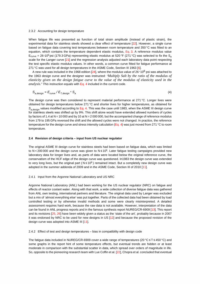
2.3.2 Accounting for design temperature

When fatigue life was presented as function of total strain amplitude (instead of plastic strain), the experimental data for stainless steels showed a clear effect of temperature [22]. However, a single curve based on fatigue data covering test temperatures between room temperature and 350 °C was fitted to an equation, which contains the temperature dependent elastic modulus, Eq. 3. A reference modulus value Ecurve = 26 X106 psi (179.3 GPa) representing elastic modulus at 520 °F (271 °C) was selected to fix the Sa scale for the Langer curve [21] and the regression analysis adjusted each laboratory data point respecting the test specific elastic modulus values. In other words, a common curve fitted for fatigue performance at 271 °C was used for all design temperatures in the ASME Code, Section III 1963 [6].

A new rule was included in the 1968 edition [24], where the modulus value of 26 X 106 psi was attached to the 1963 design curve and the designer was instructed: “Multiply Salt by the ratio of the modulus of elasticity given on the design fatigue curve to the value of the modulus of elasticity used in the analysis.” This instruction equals with Eq. 4 included in the current code.

Sa,design = Ecurve / ET,design x Sa (4)

The design curve was then considered to represent material performance at 271 °C. Longer lives were obtained for design temperatures below 271 °C and shorter lives for higher temperatures, as obtained for Sa,design values modified according to Eq. 4. This was the case until 1983, when the ASME III design curve for stainless steels was shifted up by 9%. This shift alone would have extended allowed numbers of cycles by factors of 1.4 at N = 10 000 and by 10 at N = 2 000 000, but the accompanied change of reference modulus from 179 to 195 GPa reversed the shift and the allowed cycles were not changed. In practice, the reference temperature for the design curve and stress intensity calculation (Eq. 4) was just moved from 271 °C to room temperature.

2.4 Revision of design criteria – input from US nuclear regulator

The original ASME III design curve for stainless steels had been based on fatigue data, which was limited to N < 200 000 and the design curve was given to N ≤ 106. Later fatigue testing campaigns provided new laboratory data for longer lives and, as parts of data were located below the original reference curve, the conservatism of the HCF edge of the design curve was questioned. In1983 the design curve was extended to very long lives, but the original part ( N ≤ 106 ) remained intact. But a completely new design curve was adopted in the summer addenda of 2009 and in the ASME Code, Section III of 2010 [11].

2.4.1 Input from the Argonne National Laboratory and US NRC

Argonne National Laboratory (ANL) had been working for the US nuclear regulator (NRC) on fatigue and effects of reactor coolant water. Along with that work, a wide collection of diverse fatigue data was gathered from ANL own testing, international partners and literature. The original data used by Langer was excluded but a mix of ‘almost everything else’ was put together. Parts of the collected data had been obtained by load controlled testing or by otherwise invalid methods and some were clearly misinterpreted. A detailed assessment requires hard work, because the raw data is not available. However, interpretation of the data can be found in ANL progress reports and in the famous synthesis report NUREG/CR-6909 [13]. This report and its revisions [25, 26] have been widely given a status as the ‘state of the art’, probably because in 2007 it was endorsed by NRC to be used for new designs in US [12] and because the proposed revision of the design curve was adopted into ASME III [11].

2.4.2 Effect of test and design temperatures – bias in compatibility with design code

The fatigue data included in NUREG/CR-6909 cover a wide range of temperatures (20 °C ≤ T ≤ 450 °C) and some graphs in the report hint of some temperature effects, but eventual trends are hidden or at least moderate in comparison with the substantial scatter in data, which spread over orders of magnitude in life. So, opposite to the pioneering research team with Lue Coffin et al. [22], Chopra et al. concluded that eventual

temperature effects were insignificant and could be ignored [13]. Perhaps a uniform shift of the ε-N curve was expected instead of rotation, which is the typical effect of temperature, Fig. 4.

Figure 4. Effects of material hardness and temperature typically seen as rotation of the ε-N curve.

Together with ignoring the historical roots and interest in compatibility with the ASME III codified fatigue assessment procedure, the ignoring of test temperatures resulted to an unintended or unfortunate change of the design rules. Nobody is to blame, because – as it seems – the work in ANL focused on science and new laboratory data, not on transferability of results to codes and standards. On the other hand, there must have been a high pressure in ASME for adoption of the curves endorsed by the NRC [12].

The compatibility problem goes as follows: • The regression for Langer’s reference curve as function of Sa contained a hidden assumption of

temperature effects and ensured compatibility with the design approach, Eq. 4. • Regression of the NUREG reference curve was performed as function of strain amplitude without

considering the temperature dependent translation of strain amplitudes to Sa (Eq. 4). • Finally, the elastic modulus in room temperature (ERT=195 GPa) was attached as the reference

modulus for the NUREG reference curve. This was in contrast with the ASME Code, where the reference curve had been shifted up by 9%, when the reference modulus was shifted to 195 GPa.

If the best fit regression into the NUREG data had been performed similar to the original analysis of Langer data, a higher design curve would have resulted. Firstly, the high temperature data points would have been shifted up in relation to the room temperature data. Secondly, the reference modulus for the regression curve would have been lower, one representative for an elevated temperature. If this change of design basis were made intentionally, it should have been noted. Therefore, I consider it an unintentional bias in compatibility with the ASME Code.

2.4.3 Discussion on possible consequences of the bias in compatibility with design code

Quantification of the introduced bias would require access to the NUREG raw data but – even without counting the number of data points per temperature, I dare to suggest a rough guess. In both cases, the fitted fatigue data covered wide ranges of temperatures, 20 °C ≤ Ttest ≤ 350 °C for the Langer curve and 20 °C ≤ Ttest ≤ 450 °C for the NUREG/CR-6909 curve. If the distributions of data over test temperatures and endurances were identical in both cases, the bias in stress intensity would be about 9%.

This was the amount of shift in the ASME III design curve for stainless steels in 1983 corresponding to change of reference temperature from 271 °C to room temperature and modulus from 179 to 195 GPa. A reduction of 9 % in stress intensity would have notably decreased the allowable numbers of cycles in HCF, by about an order of magnitude, when N ≈ 2 000 000. That would have a similar effect as a new penalty factor

Fbias ≈ 10 applied for the HCF edge of the curve. The slope of the design curve is lower in LCF and the penalty factor would be lower, Fbias ≤ 1.5. However, this rough estimate hints that the introduced bias may equal to component life reduction from 60 to 40 years for constant amplitude loading in range of N ≈ 10 000. Considering the efforts directed towards long term operation of NPP’s, release of the unintentional bias should be an economically attractive target for users of the ASME Code Section III for fatigue management of stainless steel piping.

On the other hand, similar bias should be avoidable, when other design codes are updated. A good example was revision of the German KTA Standard [3], where adoption of the new curve proposed in NUREG/CR-6909 [13] was avoided by dedicated experimental research focused in the stainless steel grades used in the main components of German NPP’s.

3. Fatigue curve for long lives

One more challenge in fatigue assessment of austenitic stainless steels is worth of discussing. Extension of the design curve to HCF has created generic and practical problems. It was already mentioned above how invalid or inappropriate HCF data may have affected derivation of the reference and design curves. This is a practical problem, which could have avoided through careful laboratory work and critical assessment. Furthermore, utilization of numerous run-out data raises questions. Some researchers ignore run-out points, others include them in curve fitting as failures, but neither of these options can correctly reflect the reality. This challenge and a proposed solution has been discussed by Kim Wallin [27].

3.1 Applicability of the ASME III (2010) reference curve for stainless steels

The current design curve in ASME III is a copy from NUREG/CR-6909 [13]. Even though derivation of the code curve was not presented, it is fair to consider that derivation the mean curve and design margins in NUREG/CR-6909 were adopted as such, i.e., that the ASME III reference curve for stainless steels equals with the NUREG/CR-6909 mean curve. Applicability of this reference curve in HCF and its compatibility with the source data will be discussed in the following.

Unfortunately, the source data used for the NUREG/CR-6909 mean curve is not available, but Tommi Seppänen has been able to identify almost all test results for AISI 304 and 304L [28]. Fig. 5 shows the medium and high cycle part of the data together with the mean curve, which seems to represent the LCF data reasonably well, but not at all the HCF data. Actually, it is hard to believe that this data would represent fatigue performance of material batches that are qualified for use in NPP primary piping. Strain controlled LCF tests performed and qualified according to standard procedure (ASTM E 606) should result in low scatter. An example of qualified data for relevant material was shown in Fig. 1. The scatter in fatigue lives in Fig. 5 approaches three orders of magnitude. Experimental factors such as test alignment, control mode, temperature, buckling susceptibility and variably reported run-outs are suspected to contribute in scatter and regression fitting. If anything, the ‘mean curve’ describes a lower bound for HCF. But why?

Figure 5. ‘Mean curve’ together with source data points for 304 type stainless steel collected from original sources for NUREG/CR-6909 report [28].

3.2 Regression of reference curve to a pre-selected equation

Pre-selected equations are often used for regression of fatigue data and development of design curves. Different fatigue models might be best suited for different materials, but it is convenient to use the same equation model for different materials. This is the case also with the ASME Code and NUREG/CR-6909 report, where separate design curves are provided for ferritic and austenitic steels, but the curves are fitted to the same curve model.

Experimental research at VTT has revealed pronounced endurance limit behaviour in strain controlled HCF tests for austenitic stainless steel. Comprehensive testing focused on niobium stabilized (type 347) stainless steel, Fig. 1, but the observed behaviour is not limited to this particular alloy. It is effective at least for alloy 304. Furthermore, the endurance limit behaviour is not limited to constant amplitude straining in room temperature. Increase of temperature decreases the endurance limit, but does not eliminate it. Our earlier research has indicated that – in contrast to carbon steels – the endurance limit is effective also in spectrum loading of welded 304 specimens. The modified Miner rule with S-N –curves extrapolated to low amplitudes is generally applicable for carbon steels, but not for stainless [20].

Effectiveness of the endurance limit even with variable amplitude straining was shown also for 347 type steel. Stainless steels can tolerate notable amounts of plastic strain and display broad hysteresis loops at and below the endurance limit, Fig. 3. Together with pronounced secondary cyclic hardening, this results to abrupt endurance limit behaviour. Hardening increases the endurance limit of the steel and prevents fatigue fracture, if it occurs early enough. Re-testing of four run-out specimens shown in Fig. 1 demonstrated how straining below endurance limit improved fatigue performance of the specimens in re-testing at a higher amplitude. This effect can be explained by the secondary hardening, which occurs also below endurance limit. The improvement is particularly effective, when large numbers of cycles are applied just below the endurance limit.

This abrupt endurance limit behaviour causes that regression fitting of our fatigue data results to an ε-N curve, which continues conservatively below the endurance limit, when extended beyond the range of the original Langer curve for N > 106 cycles, Fig. 1. It seems that derivation the reference curve of the current ASME Code was affected by the same problem, and probably even more severely, Fig. 5. The NUREG data bank contains more data at high amplitudes and low lives, not shown in Fig. 5. Furthermore, the regression

fitting emphasized LCF data by giving 20 times more weight to residuals in direction of ln(ε) over the residuals in direction of ln(N). The regression produces a reasonable mean curve for the LCF data, but the pre-selected equation is unable to bend the curve, when endurance limit is approached.

In summary, the NUREG/CR-6909 mean curve gives highly conservative representation of the NUREG data in HCF. This becomes obvious, when the NUREG mean curve is compared with its source data as done in Fig. 5. The suspected main reasons are:

• poor selection and quality assessment; use of partially inappropriate fatigue data • ignoring effects of test temperatures; treating all data (20°C ≤ Ttest ≤ 450°C) as RT data • generic problem of regression to a pre-selected equation, which is not suitable to describe the full

range of ε-N data from extreme LCF to extreme HCF; applying for austenite a model suited for ferritic carbon steels.

3.3 Mandatory Code Curve or Design by Analysis ?

The “design fatigue curves” included in the ASME Boiler and Pressure Vessel Code, Section III were originally attached as figures within the Article N-415 “Analysis for Cyclic Operation” together with a footnote stating that the designer shall consider, if they are applicable for the design case in hands [6]. Reading this together with the Criteria document [8] gives me an impression that the intention was not to enforce the designer to rely on the provided curves, but to help and support a designer, who does not have suitable fatigue data on the material used for fabrication of the designed equipment. Indeed, at the time it would certainly have been hard requirement for the designer to obtain sufficient material data for the applied materials. But if somebody had studied fatigue performance of the particular material batches used for construction of primary piping for a NPP, utilization of these more relevant results would have been a natural part of the “design by analysis” project.

However, for unknown reasons the design fatigue curves were later moved to an appendix labelled as “Mandatory Appendix” [29]. At the same time, the US and Finnish regulatory guides still emphasize the designer’s responsibility on applicability of the fatigue curve. When endorsing the new design curve given in the NUREG/CR-6909 report, the US NRC stated that the new regulatory guide was aimed for new designs in US only, not aimed for old plants and did not exclude use of alternative approaches, although making it clear that the easiest road is to follow the NUREG/CR-6909 [12]. According to the Finnish YVL guide 3.5 (2002) for ensuring strength of NPP pressure devices, justification was needed if the code curve was used, because “fatigue assessment shall be based on S-N -curves applicable to each material and conditions” [30].

One may question, why the design curves given in the ASME Code are discussed as the only alternatives. Already the enormous scatter in source data for the current design curve (Fig. 5) tells us that the resulting curve aims to provide a synthesis of all possible material alternatives within the group of stainless steels and is not aimed to be relevant for any particular design case. For designer of a NPP primary piping, it should be recommended to obtain at least a minimum amount of fatigue data representative for the material to be used. This may confirm applicability of the code curve or reveal need of alternative reference and pay respect to the “design by analysis” approach.

4. Conclusions

The “design by analysis” approach, which was developed for the ASME Boiler and Pressure Vessel Code, Section III, 1963 has lasted time. However, the new “design fatigue curve” for stainless steel included in the “Mandatory Appendix 1” of the current ASME Boiler and Pressure Vessel Code, Section III is not compatible with the codified design calculation and may give biased results. Conservatism of the design curve was unintentionally increased in 2009, when the curve proposed in NUREG/CR-6909 was adopted.

Cyclic response and fatigue performance of austenitic stainless steels is complex and differs notably from the performance of ferritic carbon steels. Hidden assumptions and fatigue assessment procedures tuned for carbon steels, may not optimally suit for stainless steels. In particular, extension of the original design fatigue curves to very high numbers of cycles beyond HCF may cause notable bias in design, because fatigue performance of stainless steel cannot be well presented using the same curve model for both LCF and HCF.

The new ASME III code curve is not recommended without checking relevance of the HCF part of the curve for the steel used in NPP piping.

References

1. ASME Boiler and Pressure Vessel Code, Section III, Rules for construction of nuclear facility components. Division 1 – Subsection NB Class 1 Components. ASME BPVC.III.1. NB-2015.

2. RCC-M – Design and Construction Rules for mechanical components of nuclear PWR islands – 2016 edition.

3. KTA Program of Standards, Standard No. 3201.2, Components of the Reactor Coolant Pressure Boundary of Light Water Reactors, Part 2: Design and Analysis, issue 11-2017.

4. JSME, 2016. Codes for Nuclear Power Generation Facilities, Rules on Design and Construction for Nuclear Power Plants, The First Part: Light Water Reactor Structural Design Standard, JSME S NC1-2016, Japan Society for Mechanical Engineering (JSME), 2016. (in Japanese).

5. ASTM E 606 / E606M - 12. Standard Test Method for Strain-Controlled Fatigue Testing. ASTM International, West Conshohcken, PA, 2012.

6. ASME Boiler and Pressure Vessel Code, Section III, Nuclear Vessels, 1963. Article 4, N-415 Analysis for cyclic operation, p. 18–23.

7. ASME, 1972. Pressure Vessels and Piping: Design and Analysis, A Decade of Progress, Volume One. The American Society for Mechanical Engineering (ASME) 1972. 754p.

8. ASME, 1972. Criteria of the ASME Boiler and Pressure Vessel Code for design by analysis in sections III and VIII division 2. p. 61 - 83 in reference [7].

9. ASME, 1969. First International Conference on Pressure Vessel Technology. Part I, Design and Analysis. The American Society for Mechanical Engineering (ASME) 1969. 665 p.

10. ASME, 1969. First International Conference on Pressure Vessel Technology. Part II, Materials and Fabrication. The American Society for Mechanical Engineering (ASME) 1969. 720 p.

11. ASME, 2009. ASME Code, Section III, Division 1, Appendices, Mandatory Appendix 1 Design Fatigue Curves. Addendum 2009b.

12. U.S. Nuclear Regulatory Commission Regulatory Guide 1.207, 2007. ”Guidelines for evaluating fatigue analyses incorporating the life reduction of metal components due to the effects of the light-water reactor environment for new reactors”. 7 p.

13. Chopra, O., Shack, W., 2007. Effect of LWR Coolant Environments on the Fatigue Life of Reactor Materials, Final Report. NUREG/CR-6909, ANL-06/08, Argonne National Laboratory. 118 p.

14. Asada, S., Hirano, A., Saito, T., Takada, Y. and Kobayashi, H., 2018. Development of New Design Fatigue Curves in Japan –Proposal of A New Fatigue Evaluation Method (PVP2018-84432), ASME Pressure Vessels and Piping Conference, 2018.

15. Wöhler, A., 1870. Über die Festigkeitsversuche mit Eisen und Stahl, Zeitschrift für Bauwesen vol. 20 pp. 73–106.

16. Basquin, O. H., 1910. The exponential law of endurance test. Proceedings of the American Society for Testing and Materials. 10, pp. 625–630.

17. Manson, S. S., 1953. Behavior of materials under conditions of thermal stress. National Advisory Committee for Aeronautics (NACA), Technical Note 2933, July 1953. 108 p.

18. Coffin, L. F. Jr., 1954. A study of the effects of cyclic thermal stresses on a ductile metal. Transactions of the ASME, vol. 76, No 6 August 1954, pp. 931–950. (First published in 1953 as report KAPL-853 of General Electric).

19. SAE, 1968. Fatigue Design Handbook. Advances in Engineering AE-4, Society of Automotive Engineers, Warrendale, PA, 1968. 132 p.

20. Solin J., Alhainen J., Arilahti E., Seppänen T., Mayinger W., 2019. Particular fatigue resistance of stabilized stainless steel – endurance limit, strength and ductility of fatigued steel (PVP2019-93317). Proceedings of the ASME 2019 Pressure Vessel and Piping Division Conference PVP2019, July 14-19, 2019, San Antonio, TX, USA. 7 p.

21. Langer, B.F., 1962, Design of Pressure Vessels for Low-Cycle Fatigue, Journal of Basic Engineering, 84 (3), pp. 389–399.

22. Coffin, L.F. Jr., Tavernelli, J.F., 1959. The Cyclic Straining and Fatigue of Metals, Trans. Metallurgical Society, AIME, Vol. 215, Oct. 1959, pp. 794–806.

23. Baldwin, E.E., Sokol, G.J., Coffin, L.F. Jr., 1957. Cyclic strain fatigue studies on AISI-347 stainless steel. ASTM Proceedings, vol. 57, 1957, pp. 567–586.

24. ASME Boiler and Pressure Vessel Code, Section III, Rules for Construction of Nuclear Vessels, 1968 Edition. Article 4, N-415 Analysis for cyclic operation, p. 23–28.

25. Chopra, O., Stevens, G.L., 2014. Effect of LWR Coolant Environments on the Fatigue Life of Reactor Materials, NUREG/CR-6909, Rev. 1, ANL-12/60 (Draft), U.S.NRC.

26. Chopra, O. and Stevens, G.L., 2018, Effect of LWR Coolant Environments on the Fatigue Life of Reactor Materials, NUREG/CR-6909, Rev. 1, ANL-12/60, U.S.NRC.

27. Wallin, K., 2011. Simple distribution-free statistical assessment of structural integrity material property data. Eng. Fract. Mech., 78(9), pp. 2070–2081.

28. Seppänen T., Alhainen J., Arilahti E., Solin J., 2019. Strain-controlled low cycle fatigue of stainless steel in PWR water (PVP2019-93279). Proceedings of the ASME 2019 Pressure Vessel and Piping Division Conference PVP2019, July 14-19, 2019, San Antonio, TX, USA. 11 p.

29. ASME Boiler and Pressure Vessel Code, Section III, Division 1, Appendices, Mandatory Appendix I Design Fatigue Curves, ASME, New York, 2017.

30. STUK, 2002. YVL-guide 3.5, Ensuring the strength of nuclear power plant pressure devices, issue 5.4.2002. (in Finnish, but translations exist).