Extracting Market Expectations from Option Prices: Case

1

Extracting Market Expectations from Option Prices

Extracting Market Expectationsfrom Option Prices:

Case Studies in JapaneseOption Markets

Hisashi Nakamura and Shigenori Shiratsuka

Hisashi Nakamura: Policy Planning Office, Bank of Japan (E-mail: [email protected])

Shigenori Shiratsuka: Visiting Economist from the Bank of Japan at the Federal ReserveBank of Chicago (E-mail: [email protected])

The authors are grateful to Kent Daniel, Mitsuhiro Fukao, Fumio Hayashi, Takeo Hoshi,Genshiro Kitagawa, Motonari Kurasawa, David Marshal, Yuichi Nagahara, Seisho Sato,Charles Thomas, and seminar participants at the Federal Reserve Bank of Chicago, andthe February 1999 National Bureau of Economic Research Japan Project Meeting fortheir helpful comments; and to Michio Kitahara, Laura Kutianski, and Joel Spenner fortheir extensive assistance to make this paper more readable. The opinions expressed arethose of the authors and do not necessarily reflect those of the Bank of Japan or theFederal Reserve Bank of Chicago.

MONETARY AND ECONOMIC STUDIES/MAY 1999

This paper focuses on the recently developing financial derivativesmarkets, and examines the usefulness of option prices as an informa-tion variable for monetary policy implementation. A set of optionprices provides us with information on the entire probability distrib-ution of the future values of underlying assets. Such informationenables us to examine the development of market expectations. Thepaper estimates a time series of implied probability distributionsfrom daily option prices on stock price index and long-term govern-ment bond futures in Japan. The estimation is done for a sample ofdaily closing prices for the following three periods: (1) the period of a collapsing “bubble” in the stock market in 1989–90; (2) the periodof serious stock market slump in 1992–94; and (3) the period ofincreasing anxiety in the market about a possible deflationary spiral in 1995.

Key words: Option prices; Implied probability distribution;Market expectations; Monetary policy; Informationvariables

I. Introduction

In this paper, we focus on the recently developing financial derivatives markets inJapan and examine the usefulness of option trading prices as an information variablefor monetary policy implementation. By estimating the entire probability distribu-tion of future asset prices from a set of option prices and tracking the changes in thatdistribution over time, we examine the development of market expectations and howmonetary policy has affected that development.

In general, asset prices reflect market participants’ expectations about the future.During the “bubble” era, Japan experienced large fluctuations both in asset prices andin the real economy, and market expectations seem to have played an important rolebehind the scenes. For example, market expectations became bullish during the emer-gence and expansion of the asset price bubble and remained almost unchanged evenwhen interest rates were revised upward. In such circumstances, a substantial rise ininterest rates is required in order to change market expectations. To put it differently,the effects of tight monetary policy, even accompanied by quite high interest rates, donot appear significant until market expectations change. Once such expectations havebeen revised, downward pressure on asset prices becomes extremely large because therevision of expectations intensifies the original effects of higher interest rates throughthe expansion of risk premiums.

We examine how market expectations concerning underlying asset prices areformed and how they change, using daily price data on the option markets in Japan.Specifically, we estimate the entire implied probability distribution of future values ofunderlying assets from a set of option prices with the same time-to-maturity, butwith different exercise prices. This method enables us to obtain information aboutthe dispersion of market expectations concerning asset price fluctuations, as well asabout market participants’ beliefs about the direction of market price changes and theprobability of an extreme outcome in the market.

We study the practical usefulness of this methodology through case studies involv-ing Japanese option markets. Given the data constraints, three periods have beenselected: (1) the period of the collapsing “bubble”1 from the second half of 1989 to1990; (2) the period of serious stock market slump from 1992 to early 1994; and (3) the period of increasing anxiety in the market about the deflationary spiral in1995. In each period, we consider on a time-series basis (1) how market expectationsof stock prices and long-term interest rates changed; (2) how and when the relation-ships between such market expectations and economic indicators changed; and (3) how monetary policy implementation affected such market expectations.

This paper is composed as follows. In Chapter II, we present the basic frameworkfor examining the development of market expectations. We discuss the estimationmethodology of implied probability distributions, based on the limitation in readilyavailable data in Japanese option markets. In addition, we conceptually study how we

2 MONETARY AND ECONOMIC STUDIES/MAY 1999

1. It is interesting to examine how market expectations changed during the initial period of the “bubble” era.However, due to the fact that Nikkei 225 option trading started in June 1989 and Japanese government bond(JGB) futures option trading started in May 1990, this paper must limit its scope of analysis to the period after the“bubble” burst.

can interpret the changes in market expectations from the movements of summarystatistics of the estimated implied probability distributions over time. In Chapter III,we conduct case studies for various episodes in Japanese financial markets from 1989to 1995 to examine the practical usefulness of our methodology for extracting marketexpectations. We estimate the summary statistics of the implied probability distribu-tion on a daily basis, and examine the changes in market expectations captured inestimation results, with reference to monetary policy implementation. In Chapter IV,we provide a conclusion with some policy implications. In the appendices, we showthe specific calculation methods used for the implied probability distributions, as wellas the basic framework of financial option trading in Japan.

II. Basic Framework for Analyzing Changes in MarketExpectations

Since the 1970s, methods of extracting market expectations concerning future asset prices by using derivatives trading prices have been developed and are im-proving.2 In this chapter, we first summarize various methodologies for extracting market expectations from data for financial markets. We also point out some dataproblems in conducting empirical analysis in the Japanese option markets. Then, wediscuss which method is appropriate for application to Japanese option markets.Finally, we examine the interpretation of the estimates and the bias inherent in a discrete approximation.

A. Method for Extracting Market Expectations We summarize the methodology used to extract market expectations from optionprices based on past studies.1. The method used for extracting market expectationsThere are three methods used to analyze market expectations concerning future assetprices based on financial market data.

The first method is to estimate the implied forward rates from swap rates or government bond yields, and observe expected interest rates by maturity. The secondmethod is, by using option price information, to observe the implied volatility estimatedby the Black-Scholes Model (Black and Scholes [1973]), and to evaluate the dispersionof expectations concerning future asset prices. The third method also uses optionprice information, although it goes as far as deriving the entire risk-neutral implied probability distribution of future prices of the underlying assets.

By estimating the entire expectation distribution, the third method enables us toexamine market expectations concerning future outcomes in detail. In other words, wecan obtain information about the dispersion of market expectations concerning asset pricefluctuations, as well as about market participants’ beliefs about the direction of marketprice changes and the probability of an extreme outcome in the market. This method is

3


2. A comprehensive survey of these methods can be found in Neuhaus (1995), Söderlind and Svensson (1997),Bahra (1996, 1997), and Oda and Yoshiba (1998).

deemed useful for close monitoring of the impact of monetary policy on marketexpectations. In the following, we will discuss rather extensively the specifics of how toestimate the implied probability distribution. 2. Estimation methods for the implied probability distributionThe methods used to estimate the implied probability distribution fall into two categories according to whether or not they ex ante assume a specific distributionfunction.

Models that ex ante assume a specific distribution function include a model whichassumes underlying asset prices follow a jump probability distribution process3 (Malz[1996]; Bates [1991, 1996, 1997]), and a model which assumes a probability densityfunction of underlying asset prices that follows a mixture of some lognormal distribu-tion (Melick and Thomas [1997]; Bahra [1996]; Söderlind and Svensson [1997];Söderlind [1998]). There are various other possible models that assume differentprobability distribution patterns. However, in the actual analysis, it is impossible torecognize ex ante the probability distribution of the underlying asset prices, and thusthese models inherit the deficiency of not being able to preclude arbitrariness fromthe estimation process.

Other less-constrained models, in which a specific distribution pattern is notassumed ex ante, include a method of directly estimating the probability distributionof option price data by using finite difference methods4 (Breeden and Litzenberger[1978]; Neuhaus [1995]), a method that utilizes a smoothing curve called the splinefunction (Oda and Yoshiba [1998]), and a method that applies kernel regression (Aït-Sahalia and Lo [1998]).

B. Application to Japanese MarketsNext, based on the features of Japanese option markets, we examine which estimationmethod to apply in our study. We use the Nikkei 225 option (a European-typeoption) and the Japanese government bond (JGB) futures option (an American-typeoption).5 The underlying assets of those options are the Nikkei 225 Stock Average


3. It is not necessarily logical to assume that asset prices such as stock prices change continuously, since social andeconomic information emerges intermittently. In finance theory, a jump probability distribution process is oftenused to cope with discontinuous price changes. In detail, there are two types in a jump distribution process: a purejump probability distribution process and a diffusion probability distribution process. A pure jump probabilitydistribution process assumes that price changes follow a discrete Poisson process. A diffusion probability distribu-tion process assumes that price changes follow a weighted average of the Wiener process (continual price changes)and the Poisson process (intermittent price changes).

4. Finite difference methods convert differential equations into a set of difference equations and the difference equations are solved iteratively, and are widely used to solve the partial differential that represents the derivativesprice. To illustrate the approach, we consider a first-order differentiable continuous function f (S ). A number ofequally spaced stock prices are chosen as S1, S2, . . . , Sk , . . . , and the width of the space as ∆S. The first-order differential ∂f /∂S S=Sk at point Sk can be approximated as a forward difference approximation { f (Sk +1) – f (Sk)}/∆S, a backward difference approximation { f (Sk) – f (Sk –1)}/∆S, and a central difference approximation { f (Sk +1) – f (Sk –1)}/2∆S. Among these, this paper adopts the central difference approximation, which is the one with a more symmetricalapproximation. For details on the finite difference methods, see Chapter 15 of Hull (1997).

5. We apply the calculation method for the European-type option explained in Appendix 1 to the JGB futuresoption that is the American-type option. In general, calculation of the American-type option is more complicatedthan that of the European one, since buyers can arbitrarily exercise the option. However, Chen and Scott (1993)showed that the American-type interest rate futures option can be priced as the European-type option if sellerssubmit margins and the margins are marked to market every day. Since the JGB futures option applies a similarmargin system, we believe that there should be no problem in treating it as the European-type option.

(hereafter, Nikkei 225) and the 10-year JGB futures, respectively (see Appendix 2 forthe outline of each transaction).6

1. Limitations of available data for Japanese option marketsSome cautions are in order concerning the empirical analysis of Japanese option data.First, only a small number of opened strike prices are available. Since there is verysmall trading volume for the in-the-money (ITM) strike prices, reliability of priceinformation is not entirely satisfactory.

Second, there is a limitation involved in using closing price data. Namely, usingclosing price data will not guarantee that the option premiums of different strikeprices were traded at the same time. If there are substantial time differences in thetraded times of closing prices across different strike prices, arbitrage may not functionthoroughly. In this case, the probability density of the implied probability distributionwill inherit certain biases.

Third, it has been pointed out that, during the transitional period of most activelytraded contract months, trading prices will not fully reflect market expectations concerning future outcomes. As a result, the most actively traded contract monthmight not be the contract month with the largest trading volume.2. Strategy to deal with the data problemsOne possible strategy for overcoming the problems mentioned above is to imposesome restrictions to guarantee that the results give a reasonable probability distribu-tion, such as assuming a mixture of some lognormal, and a fitted spline function.Another strategy is to apply a simple discrete approximation method to carefullysorted data. We have used the latter strategy to estimate a time series of implied probability distributions with the following devised data treatment.7

First, we have applied a simple discrete approximation method. It is difficult toget a robust estimation result when we apply a complicated methodology to a smallsample. Considering the lesser observations across the different strike prices in theJapanese option markets, advanced methodology is not necessarily required. In addition, a simple methodology may even give rise to clearer policy implications.

Second, we have used price data regarding both put and call options that are at-the-money (ATM) and out-of-the-money (OTM). We first calculate two pro-bability distributions from the option premium for call and put options separately,then combine two probability distributions at the ATM strike price to form the complete probability distribution (see Figure 1 for the illustration of the estimationprocedure). In this sense, our methodology has the merit of effectively utilizing trading price information by making the ATM strike price the boundary and usingboth put and call options on the OTM side. Therefore, there is an advantage in estimating the implied probability distribution using limited quotations of optionpremiums across different strike prices, such as Japanese option markets.

5


6. A Euroyen interest rate futures option has also been traded in Japan since July 1991, although due to the short overlapping period for the purpose of our analysis and the rather low trading volume, we judged that the credibilityof price data on the Euroyen interest rate futures option markets is questionable and thus excluded it from our study.

7. Of course, it should be noted that a bias might be introduced, even though we apply a simple method to carefullysorted data, especially when the expiration date of the option approaches and the number of traded strike prices inthe markets becomes smaller. Further research is required on the robustness of estimation results across the differentmethods for estimating implied probability distributions.


25Percent Put + call

20

15

10

5

0

Combine at the ATM

15,250 15,750 16,250 16,750 17,250 17,750 18,250

1,000Yen Put

ATM ATM

CallYen

800

600

400

200

0

1,000

800

600

400

200

015,000 15,500 16,000 16,500 17,000 16,500 17,000 17,500 18,50018,000

Option premium

Percent Put Percent Call80

60

40

20

0

80

60

40

20

0

Implied probability distribution

15,250 15,750 16,250 16,750 16,750 17,250 17,750 18,250

ATM

ATM

ATM

Third, we have excluded mispriced observations, such as those which result in anegative probability density, in estimating the complete probability distribution. Aspreviously mentioned, using closing price data does not guarantee that the optionpremiums of different strike prices were traded at the same time, and arbitrage maynot function thoroughly.

Fourth, we have excluded from our analysis as much as possible the data of thefinal week of each contract month. As a result, the most actively traded contractmonth might not be the contract month with the largest trading volume.

C. Framework for Interpretation of Changes in Market ExpectationsIn this paper, we examine the changes in market expectations by using a time series offour summary statistics or moments (mean, standard deviation, skewness, and excess kurtosis) of the estimated implied probability distributions. Then, after defining the four

Figure 1 Estimation Method for Implied Probability Distributions

summary statistics, we discuss how we can interpret changes in market expectations fromchanges in these statistics. In addition, we discuss the possibility of biases induced by thediscrete approximation method, which we employ in this paper.1. Summary statistics and shape of distributionWe employ a time series of summary statistics of estimated implied probability distri-butions to investigate the changes in market expectations. Specifically, we obtainmean, standard deviation (Stdv), skewness (Skew), and excess kurtosis (Ex-Kurt)from the histogram of implied probability distribution.

Since stock and bond prices are both positive values, even when market expecta-tions belong to the same population corresponding to the same probability space, theexpectation distribution of future assets will follow a lognormal distribution. In otherwords, the distribution is expected to be skewed to the right. However, it is not convenient to use a lognormal distribution as a benchmark for evaluating the size ofthe above summary statistics. Therefore, we calculate these summary statistics byusing the strike price converted into a logarithm, and employ a normal distributionas the benchmark for evaluating the four summary statistics. As shown in Appendix1, if we use p (Ki ) obtained by the formulations (A.14) and (A.15), the four summarystatistics can be shown as follows:

ln(Ki ) + ln(Ki+1)Mean = ∑ p(Ki ) (1)2

ln(Ki ) + ln(Ki+1) 2

Stdv = √ ∑ ( – Mean) p(Ki ) (2)2


Skew = ∑( – Mean)p(Ki )/Stdv 3 (3)2


Ex-Kurt = ∑( – Mean)p(Ki )/Stdv 4 – 3. (4)2

While the mean of the estimated risk-neutral implied probability shifts in parallelwith the size of risk premium compared with the true probability distribution, therisk premium itself is difficult to estimate.8 Thus, in the following, we focus onchanges of moments higher than the first, i.e., mean, and examine their movementsover time.9

7


8. The model used in this paper assumes a risk-neutral world, while market participants in the actual market are notnecessarily risk-neutral. In addition, it is likely that the risk preferences of market participants change over time. In that case, the (risk-neutral) implied probability distribution, estimated under the assumption of risk-neutral valuation, will differ from the true probability distribution. However, Cox and Ross (1976) claimed that, com-pared with the true probability distribution, the risk-neutral implied probability distribution shifts in parallel withthe size of the risk premium, and thus will not affect moments higher than the second.

9. As Bates (1991) and others have pointed out, it is generally known that the standard deviation decreases as the maturity date of the contract is approached. Therefore, we try to control the impact of changes in time-to-maturity on the estimated time series of the standard deviation by multiplying the square root of (360/time-to-maturity) to obtain the annual rate.

The changes in market expectations captured by the movements of each summarystatistic can be summarized as follows. From the standard deviation, we can see thedispersion of distributions, that is, how wide the market expectations are, which cannot be distinguished by only observing the mean.

Skewness is a statistic that shows the extent of asymmetry of the distribution: it iszero in the case of a symmetric distribution such as the normal distribution, positivewhen distribution is skewed to the right, and negative when skewed to the left(Figure 2).


–30

0.05

0.10

0.15

0.20

0.25

0.30

0.35

0.40

0.45Probability density f (x)

xSource: Yoshiba (1996).

Skew > 0 Skew = 0 Skew < 0

–2 –1 0 1 2 3

Figure 2 Skewness

–30

0.050.100.150.200.250.300.350.400.450.50

x

Ex-Kurt > 0Ex-Kurt = 0

Ex-Kurt < 0

–2 –1 0 1 2 3

Probability density f (x)

Source: Yoshiba (1996).

Figure 3 Excess Kurtosis

Excess kurtosis is a statistic that shows the degree of sharpness of a probabilitydensity near its center and the likelihood of extreme outcomes: it is also zero in thecase of a normal distribution. When positive, probability density at the center of distribution is high, and thus the shape of the distribution becomes sharp at the center and also fat-tailed. When negative, the distribution becomes flat at the centerand light-tailed (Figure 3).

It might be worth explaining in detail what kind of information about changes inmarket expectations can be captured by the shift in the excess kurtosis. As the excess kurtosis increases, (1) the extent of sharpness at the center will increase; and (2) the degreeof fatness at the tail will increase. If we compare such changes intuitively with an economic agent’s expectation formation process, two interpretations are possible: (1) anagent is expecting that asset prices are not likely to change from the center of distribu-tion; or (2) an agent is expecting that asset prices are likely to change substantially, namely,to take outlier values. Therefore, it is not clear whether we can draw any implications foreconomic agents’ expectations by just observing the changes in the excess kurtosis.

In order to decide which of the above two interpretations we should take, we needto combine excess kurtosis with standard deviation, a measure that represents the dispersion of the whole distribution. Specifically, when there is no change or decreasein the standard deviation, an increase in the excess kurtosis will sharpen the probabil-ity density near its center, and can be interpreted as an increase in economic agents’ confidence in the current market level. On the contrary, when there is an increase inthe standard deviation, a rise in the excess kurtosis will make the tails of distributionfatter, and can be regarded as indicating a higher possibility of extreme outcomes.Such interpretations are summarized in Table 1.

9


Table 1 Interpretation of Fluctuation in Standard Deviation and Excess Kurtosis

Excess kurtosis

Rise Fall

Larger risks on price changes Larger risks on price changes

Rise + +stronger expectation of weaker confidence concerning

Standard an extreme outcome the current price leveldeviation Smaller risks on price changes Smaller risks on price changes

Fall + +stronger confidence concerning weaker expectation of

the current price level an extreme outcome

Early stage of rise in market level Recovering stability in market level

Probability density

Strike price

Probability density

Strike price

Stdv: riseSkew: increasingly negativeEx-Kurt: rise

Stdv: fallSkew: decreasingly negativeEx-Kurt: fall

Figure 4 Changes in Distribution of Market Expectations during the Rise in Market Level

2. Interpretation of changes in summary statisticsWhen the market level fluctuates, how do the above summary statistics react, andthrough them, what kinds of changes in market participants’ expectations can begrasped? Figure 4 shows an image of typical changes in probability distribution when the

market level is rising. As shown in the left part of the figure, the standard deviation andthe excess kurtosis rise and the skewness shifts in a negative direction. Subsequently, aftera short time and with gradually recovering stability in the market, both the standard deviation and the excess kurtosis decline, the extent of negative shift of the skewnessshrinks, and the distribution will approach a normal distribution.10

We interpret the changes in implied probability distribution as capturing thechanges in the expectations of a representative investor in the market.11 Namely, arepresentative investor’s expectation of stock price fluctuations will follow a normal distribution in the long run, although it will exhibit stronger confidence in either a riseor a fall in the short run reflecting factors such as the current phase of the business cycle.For example, in the early phase of a market rise, the representative investor will expect afurther improvement in companies’ performances and thus expect the market to rise forthe time being, resulting in a swelling of the right side of the expectation distribution.Consequently, the distribution will be skewed to the left, and the skewness becomes nega-tive. In addition, since the risk of price fluctuations increases, the standard deviationincreases, the fatness of the left tail increases relatively, and the excess kurtosis rises.

In summary, for short-term changes in the market, skewness will change in thedirection opposite to that of the market level, while the standard deviation and theexcess kurtosis increase. The changes of these three summary statistics show howmarket expectations have responded to external shocks, and thus tell us the magni-tude of any unexpected shocks that hit the market. In addition, by examining thelength of the adjustment period needed to regain the original position, we can see towhat extent market expectations have been smoothly adjusted. 3. Biases from discrete approximationWe have so far discussed how to interpret each summary statistic by assuming a continuous probability distribution. However, the actual analytical method, whichwe employ in this paper discretely, approximates a continuous distribution based on anidea called the finite difference method with discretely observed option prices. Thus, thereis a possibility that discrete approximation may introduce errors into each summary sta-tistic. We simulate the errors of the discrete approximation against the continuousstandardized normal distribution, when the center of the distribution is shifted.12

Figure 5 is an illustration that shows the extent of errors introduced when thecenter of the distribution is shifted by 0.4 times one standard deviation from theoriginal center located in the center of the interval in the histogram. The normal distribution shifts from the dark to the light solid line, and the discrete approxima-tions of the distribution before and after the shift are shown as histograms of the darksolid line and of the shadowed area, respectively.13


10. When the market level is falling, the skewness will shift in a positive direction, while the standard deviation andthe excess kurtosis generally change as they do in the case of a market rise. In the following, therefore, we canequally discuss the case of a market fall by changing the sign of skewness.

11. In interpreting the changes in implied probability distribution from the viewpoint of economic theory, we owemuch to our discussion with Takeo Hoshi.

12. We owe much to our discussions with Genshiro Kitagawa, Yuichi Nagahara, and Seisho Sato in dealing with errorsin discrete approximation.

13. Since the actual fluctuation of asset prices is, in general, asymmetric and fat-tailed, we often focus on excess kurtosisthat shows the fatness of the tails in distribution. However, taking account of the fact that errors of discrete approximationare largest in excess kurtosis in our analytical framework, this summary statistic requires wide interpretation.

In this case, although the original probability distribution is a symmetric normaldistribution, the discretely approximated distribution is skewed to the left becausethe center of the original distribution has shifted to the right from the center of theinterval in the histogram. When we see the errors in each summary statistic shown inthe box in Figure 5, errors of the mean and the standard deviation are small and donot increase that much as the center of the distribution shifts. In contrast, errors inthe skewness and excess kurtosis will increase slightly as the center shifts.

Our next simulation, shown in Figure 6, examines to what extent the approxi-mated error changes according to the shift in the center of distribution.14 Errors inmean are almost negligible: in the standard deviation they are about 0.04 points,

11


14. This simulation continues to assume the intervals of the discrete approximation as one standard deviation, anddepicts how each summary statistic disperses from that of a standard normal distribution when the center of thedistribution moves by an interval of 0.01 times one standard deviation.

–3.5 –3.0 –2.5 –2.0 –1.5 –1.0 –0.5 0 0.5 1.0 1.5 2.0 2.5 3.0 3.50

0.05

0.10

0.15

0.20

0.25

0.30

0.35

0.40

0.45Probability density

Discrete (time = 0)

Discrete (time = 1)

0.4 times of standard deviation

Distance from the center measured by standard deviation

Continuous (time = 0)

Continuous (time = 1)

Mean: 0.00 → 0.40 (0.00 → 0.40)Stdv: 1.04 → 1.04 (1.00 → 1.00)Skew: 0.00 → –0.02 (0.00 → 0.00)Ex-Kurt: –0.06 → –0.09 (0.00 → 0.00)

Figure 5 Bias in Discrete Approximation

Notes: 1. This chart shows errors in the discrete approximation of standard normal distribution,when the center of the distribution is shifted from the center by 0.4 times one standarddeviation.

2. Figures in the box show the impact of shift in the center of distribution on summarystatistics. Figures in parentheses indicate summary statistics in original standard normaldistributions.

0 0.1 0.2 0.3 0.4 0.5–0.12

–0.10

–0.08

–0.06

–0.04

–0.02

0

0.02

0.04

0.06Deviation from normal distribution

Changes in average measured by standard deviation

StdvEx-Kurt

MeanSkew

Figure 6 Simulation of the Impact of Discrete Approximation

Note: This chart shows dispersion of various summary statistics of the discrete approximation by the interval of onestandard deviation from those of standard normal deviation, as the center of the distribution moves.

although they are stable and do not increase as the original distribution shifts awayfrom the center; errors in skewness increase as the original distribution shifts awayfrom the center, although the size is only 0.04 points at the largest. In the meantime,errors in excess kurtosis increase from 0.06 to 0.10 points, and when the original distribution shifts from the center more than 0.25 times one standard deviation, theerror starts to increase by a larger amount.

So what are the effects of such discrete approximation errors on the actual estima-tion? In the actual option transaction, intervals of strike prices are set constantregardless of the price level of the underlying assets or time-to-maturity. Therefore,effects of the above errors based on the standard deviation will change as stock pricesand times-to-maturity change.

In order to see this, we have estimated a matrix (Table 2) showing what size of stockprice volatility (i.e., the annualized standard deviation) corresponds to half of thestrike price interval (¥250) under different combinations of stock price (rows) and time-to-maturity (columns). When the stock price level is more than ¥28,000, and as long asthe time-to-maturity of the option is more than five days, stock price volatility will notexceed 0.25 times one standard deviation,15 the level at which effects of errors in discreteapproximation start to increase. However, when the stock price falls to the level of¥24,000, stock price volatility exceeds 0.25 times one standard deviation even with a time-to-maturity of more than 20 days, and thus the effects of errors may become substantial.16


Table 2 Impact of Changes in Stock Price Level and Time-to-Maturity toApproximation Errors

Stock price Time-to-maturity (days)(yen) 5 10 15 20 25 30 35 40 45

14,000 15.2 10.7 8.7 7.6 6.8 6.2 5.7 5.4 5.1

16,000 13.3 9.4 7.7 6.6 5.9 5.4 5.0 4.7 4.4

18,000 11.8 8.3 6.8 5.9 5.3 4.8 4.5 4.2 3.9

20,000 10.6 7.5 6.1 5.3 4.7 4.3 4.0 3.8 3.5

22,000 9.6 6.8 5.6 4.8 4.3 3.9 3.6 3.4 3.2

24,000 8.8 6.3 5.1 4.4 4.0 3.6 3.3 3.1 2.9

26,000 8.2 5.8 4.7 4.1 3.6 3.3 3.1 2.9 2.7

28,000 7.6 5.4 4.4 3.8 3.4 3.1 2.9 2.7 2.5

30,000 7.1 5.0 4.1 3.5 3.2 2.9 2.7 2.5 2.4

32,000 6.6 4.7 3.8 3.3 3.0 2.7 2.5 2.3 2.2

34,000 6.2 4.4 3.6 3.1 2.8 2.5 2.4 2.2 2.1

36,000 5.9 4.2 3.4 2.9 2.6 2.4 2.2 2.1 2.0

38,000 5.6 3.9 3.2 2.8 2.5 2.3 2.1 2.0 1.9

40,000 5.3 3.8 3.1 2.7 2.4 2.2 2.0 1.9 1.8Notes: 1. Figures in this table indicate how large volatility (i.e., annualized standard deviation) of stock prices corre-

sponds to half of the interval between adjacent exercise prices, that is, ¥250.2. Shaded figures are those that exceed the mean daily volatility (annualized) of stock prices (from 1989 to

1996) multiplied by 0.25 (22.3 × 0.25 = 5.566).

15. In calculating the standard deviation, which serves as the evaluation criterion, we used daily volatility (annual-ized) of the Nikkei 225 during 1989–96.

16. In 1989, when Nikkei 225 option trading started, the Nikkei 225 was over ¥30,000, and thus might not haveintroduced any large errors even with ¥500 strike price intervals. However, because of the subsequent fall in stockprices, intervals of strike prices have become relatively wide. The estimate in this paper can be interpreted toimply the necessity of reviewing the strike price intervals.

An often-used approach to analyze changes in market participants’ expectations is to compare the distribution shapes themselves before and after certain events,because these are easy to understand. However, based on the above simulation, itshould be noted that there is a risk of misreading the discrete approximation errors as precise indicators of changes in market expectations, since this approachdepends on option prices at a specific point in time. In addition, as previously mentioned, option trading in the Japanese markets features only a few strike pricesand the market is still not deep enough.17 Therefore, if we interpret the changes inimplied probability distribution by relying on the distribution shapes at a specificpoint in time, changes explained in this way are subject to disturbing factors such astemporary mispricing.

Based on the above discussion, this paper tracks a time series of summary statistics (thestandard deviation, skewness, and excess kurtosis) of implied probability distributions toexamine the changes in financial market participants’ expectations.18 In addition, takinginto account the fact that the intervals of the strike prices are relatively large and thuslikely to introduce errors by discrete approximation, we observe the general trend ofchanges in each summary statistic which is shown by the distribution shape, andfocus on examining the relationship between asset price movements and changes in distribution shape.

III. Development of Financial Markets and Market Expectations

We will now apply the method of analysis introduced in the previous chapter to periods in which financial markets have experienced large fluctuations, and examinehow market participants’ expectations have changed in the course of those events.Specifically, we will consider three periods: (1) the second half of 1989 to 1990, theperiod of the collapse of the “bubble” in the stock market; (2) 1992 to the beginningof 1994, the period of record-low stock prices; and (3) 1995, the period of increasinganxiety in the market about a possible deflationary spiral.

A. OverviewInstead of proceeding directly with a case study of each period, we first summarizethe development of financial markets—short- and long-term interest rates, foreignexchange rates, and stock prices—as well as the condition of the Japanese economy and the responses of monetary policy. We also try to draw a rough image of how the implied probability distribution extracted from the Nikkei 225 options haschanged over time.

13


17. While normally there are about five traded strike prices in the Nikkei 225 options, the S&P 500 stock priceindex options have some 30 prices.

18. There are various ways of examining the time-series changes in estimated implied probability distribution. Forexample, Söderlind (1998) tried to evaluate the market expectations for British monetary policy during theEuropean currency crisis in 1992, and instead of analyzing several statistics that show the distribution shape, useda 90 percent confidence interval around a risk-neutral expected value.

1. Development of financial markets and monetary policyBased on Figure 7, we first review the development of financial markets and monetary policy from the second half of 1989 to 1995.

In the period of the collapsing “bubble,” the Bank of Japan initiated a preemptivetightening of monetary policy on May 31, 1989, followed by a second tightening inmid-October and a third on December 25, four days before the Nikkei 225 reachedits peak. Even after the stock price peaked, this tight policy stance was maintaineduntil mid-1991, when the discount rate was lowered from 6.0 percent to 5.5 percenton July 1 to end the two-year tightening period. In the meantime, the uncollateral-ized overnight call rate moved roughly in parallel with the discount rate, while the10-year government bond yield sometimes moved in the opposite direction to that of


Source: Bank of Japan, Economic Statistics Monthly.

Figure 7 Development of Financial and Foreign Exchange Markets

[1] Long- and Short-Term Interest Rates

9

8

7

6

5

4

3

2

1

01989 90 91 92 93 94 95 96

Uncollateralized call rates (overnight)

Government bonds (10 years)

Official discount rate

Percent

[2] Foreign Exchange Rates and Stock Prices

40,000

35,000

30,000

25,000

20,000

15,000

10,000

180

160

140

120

100

80

601989 90 91 92 93 94 95 96

Nikkei 225 Stock Average (left scale)

Foreign exchange rate (right scale)

Yen Yen/US$

the call rate. With regard to the stock prices, after reaching its peak at ¥38,915 in December 1989, the Nikkei 225 tumbled during the period from February to May 1990. After a temporary rebound, it fell again from the latter half of 1990 to a level below ¥20,000. Subsequently, the Nikkei 225 rallied to ¥26,000, although it dropped to some ¥22,000 in the second half of 1991. The EconomicPlanning Agency reported that the boom in the Japanese economy had peaked out in April 1991.

An easy monetary policy continued toward mid-1992, when stock prices bottomed. During the period from late 1991 to mid-1992, the Bank of Japan cut theofficial discount rate four times, from 5.5 percent to 3.25 percent, and market interestrates declined, reflecting the cuts in the discount rate and the deceleration of the economic expansion. The uncollateralized overnight call rate dropped below 5 percent in April 1992 and long-term interest rates declined accordingly. In themeantime, the stock market dropped substantially, reflecting the downward revisionsof companies’ performances toward early April 1992. It suffered a further decline dueto increasing uncertainty about the future of the economy, and in August it fell below¥15,000 for the first time in the post-“bubble” period. The Nikkei 225 showed aslight recovery with the planning of the Emergency Economic Policy Package at end-August, moved around the ¥17,000 level in early 1993, and rose rapidly to above¥20,000 in March, when an additional fiscal stimulus package was confirmed.

Due to the prolonged recession, the easy monetary policy continued in 1993,with the official discount rate cut to 2.5 percent in April and to 1.75 percent inSeptember. Short-term interest rates consistently declined, while long-term interestrates temporarily rose in response to favorable economic indicators in the spring,although they then declined sharply until the beginning of 1994 due to the yen’sappreciation and weak prospects for the economy. Reflecting optimistic views on theeconomy, stock prices rose in the spring of 1993, fell during October and November,and recovered slightly thereafter. In the foreign exchange market, the yen rapidlyappreciated toward the summer of 1993.

In 1995, anxiety about deflation intensified. In the foreign exchange market, theyen started to appreciate rapidly after February 1995, reflecting the disturbances suchas the Mexican Peso Crisis, and the appreciation accelerated to temporarily break the ¥80 level against the U.S. dollar in mid-April. The market’s forecast about thefuture of the Japanese economy weakened, and the Nikkei 225 fell below ¥15,000 inmid-June 1995. Under these circumstances, the Bank of Japan continued its easymonetary policy by announcing at end-March that it would let the uncollateralizedovernight call rate decline, on average, to a level slightly below that of the official discount rate, and lowered the official discount rate from 1.75 percent to 1.0 percentin April 1995. Subsequently, short-term interest rates further declined to a record-lowlevel reflecting a policy of additional easing in July (when the uncollateralizedovernight call rate was allowed to decline further) and September (when the officialdiscount rate was cut from 1.0 percent to 0.5 percent). Long-term interest rates alsoremained at low levels. In the foreign exchange market, after July, policy coordinationamong leading countries led the yen to modify its overshoot to around the ¥100 levelagainst the U.S. dollar. The Nikkei 225 also rebounded after July.

15


2. Movements of expectations in the stock marketNow we turn to the changes in market expectations during this period by observing thechanges in summary statistics about the implied probability distribution estimatedfrom option prices (Figure 8).

We can see that the standard deviation increased when stock prices droppedsharply. This increase in standard deviation is notable in four phases: (1) from end-1989, when the Nikkei 225 reached its peak, to the fall of 1990, when it fellbelow ¥20,000; (2) from mid-1991 to mid-1992, when the Nikkei 225 fell below¥15,000 for the first time in the post-“bubble” period; (3) from the second half of1993 to early 1994; and (4) from the beginning to the middle of 1995, when the yenrapidly appreciated and anxiety about a possible deflationary spiral increased. Inaddition, the level of the standard deviation increased after end-1989, which seems toimply that market participants became more conscious of the risk of price volatilityafter the stock market entered its adjustment phase.

The skewness shifted toward a negative value when stock prices were rising, andtoward a positive value when stock prices were falling. For example, when we look indetail at the second half of 1989, there were three phases (the second half of July, thesecond half of September, and from the second half of November to end-December)in which the rise of the Nikkei 225 accelerated. The skewness shifted from slightlypositive to negative in all three cases. During the period around October 1991 whenstock prices tumbled, the skewness shifted back to a positive value. This relationshipbetween the market fluctuation and skewness is consistent with our hypothesisshown in the previous chapter that the adjustment speed of participants’ confidenceon the future price will become asymmetric between the upper and lower directionsof the current market level according to the phases of market fluctuation. The excess kurtosis was negative on average, although the extent of negativity shrank orsometimes turned positive under large price fluctuations and also showed a jump inthe case of an extreme price change.

Table 3 calculates the coefficients of correlation between the daily changes of stock prices and the summary statistics for implied probability distributions. The table confirms the above observations on the movements of summary statisticsin accordance with fluctuations in market levels. The skewness showed a relativelyhigh negative correlation with the changes in stock prices. The standard deviationand excess kurtosis indicated a positive correlation with the absolute value of dailychanges in stock prices.

Table 4 compares the summary statistics for implied probability distributions withthose for the distribution of daily changes in stock prices. Over the sample periods,the mean was almost identical and the standard deviation showed a similar tendency,while the skewness and excess kurtosis were quite different. The skewness was positive in many periods in the time-series data, while, except for 1992, it was negative in the implied probability distribution. The excess kurtosis was consistentlypositive and formed a fat-tail distribution in the time-series data, while it was negative in the implied probability distribution.

In the following sections, we analyze the changes in financial market expectationsby examining the time series of the summary statistics of implied probability


17


Figure 8 Stock Prices and Market Expectations (Overview)

[1] Nikkei 225 Stock Average

141210

86420

–2–4–6–8

–101989 90 91 92 93 94 95 96

Daily changes (left scale)

Stock price level (right scale)

Percent40,000

35,000

30,000

25,000

20,000

15,000

10,000

Yen

[2] Standard Deviation

0.4

0.3

0.2

0.1

01989 90 91 92 93 94 95 96

[3] Skewness

2

1

0

–1

–2

–31989 90 91 92 93 94 95 96

[4] Excess Kurtosis

86420

–2–4

1989 90 91 92 93 94 95 96

distributions for the following three periods: (1) the second half of 1989 to the firsthalf of 1991, the period of the collapse of the “bubble” in the stock market; (2) 1992to the beginning of 1994, the period of serious stock market slump; and (3) 1995,the period of increasing anxiety in the market about a possible deflationary spiral.

B. During the Collapse of the “Bubble”First, with respect to the period of the collapsing “bubble,” we examine the threeperiods that show striking movement from the viewpoint of stock price and interestrate fluctuation as well as monetary policy operation: (1) from the introduction of the Nikkei 225 options to December 29, 1989, when stock prices peaked; (2) from the peak of stock prices to April 1990, when stock prices tumbled below ¥30,000; and (3) from June to October 1990, when the Nikkei 225 rapidlyfell after a short rebound to a level temporarily below ¥20,000. The points at issuehere will be how strongly confidence changed and how monetary policy responsesaffected such changes.


Table 4 Comparison of Summary Statistics: Distribution of Daily Changes andImplied Probability Distribution

Daily changes Implied probability distribution

Mean Stdv Skew Ex-Kurt Mean Stdv Skew Ex-Kurt

Full sample –5.663 23.197 0.443 5.348 –5.753 16.411 –0.274 –0.603

1989 31.377 8.321 –0.346 1.323 31.206 6.285 –0.452 –0.866

1990 –39.233 32.447 0.829 5.751 –38.632 15.359 –0.151 –1.140

1991 –3.700 21.066 –0.065 2.508 –2.386 13.311 –0.352 –1.046

1992 –25.286 29.785 0.436 1.064 –25.185 23.188 0.051 –0.569

1993 2.956 20.505 0.252 1.813 3.234 17.362 –0.203 –0.362

1994 13.406 17.753 0.867 8.910 10.410 16.227 –0.345 –0.453

1995 0.739 22.503 0.122 2.304 0.348 19.230 –0.362 –0.126

1996 28.048 14.657 0.698 2.897 29.271 14.918 –0.713 –0.073

Notes: 1. Mean (daily changes) and standard deviation are annualized.2. The sample period for 1989 is the second half of the year and that for 1996 is the first half of

the year.

Table 3 Correlation between Market Level Changes and Summary Fluctuations

Mean Stdv Skew Ex-Kurt

Full sample 0.775 0.227 –0.347 0.081

1989 0.544 0.102 –0.408 0.113

1990 0.663 0.113 –0.532 0.160

1991 0.725 0.008 –0.435 0.146

1992 0.801 0.143 –0.347 0.182

1993 0.849 0.078 –0.350 0.301

1994 0.871 0.406 –0.234 0.167

1995 0.894 0.072 –0.309 0.011

1996 0.813 –0.126 –0.297 0.017

Notes: 1. Figures in the table are the coefficients of correlation between daily changes of the Nikkei225 (closing price) and summary statistics. With respect to standard deviation and excesskurtosis, we take absolute values for the daily changes of the Nikkei 225.

2. The sample period for 1989 is the second half of the year and that for 1996 is the first half ofthe year.

1. Prior to the peak of the Nikkei 225 (June–December 1989)First, we will take up the period ranging from the introduction of the Nikkei 225options to December 29, 1989, a day when stock prices peaked.

Figure 9 shows the changes in stock price expectations during this period. Asmentioned, in the second half of 1989 toward the peak of the Nikkei 225, there werethree phases (the second half of July, the second half of September, and from the second half of November to end-December) in which the rising pace of the Nikkei225 accelerated. In each period, the skewness declined from around zero to a negativevalue, the standard deviation remained almost constant, and the excess kurtosismoved up and down substantially when stock prices soared.

When we examine these periods with reference to monetary policy up to the rise in the official discount rate from 3.25 percent to 3.75 percent on October 11,the standard deviation and skewness both increased, and the excess kurtosis alsoincreased while showing volatile ups and downs. From such changes in the shape of the distribution, we conjecture that, while the forecast for the official discount rate rise prevailed, the risk of stock price changes also intensified. Therefore, a viewthat the rise in the official discount rate was already incorporated in the market sentiment at that time is not consistent with the movement of the estimated implied probability distribution.

If we focus on the movement of the standard deviation, we can see that there was a large jump at the time of shifts in the most actively traded contract monthsafter July 1989. In particular, at the time of shift from the October contract to the November contract in 1989 (shown in Figure 9 as a vertical dashed line), notonly was the magnitude of the jump large but the shift itself was delayed until immediately before the exercise date. This movement in the standard deviation canbe interpreted as indicating that while the forecast for the official discount rate riseprevailed, the risk of short-term stock price changes became large, and thus resultedin a delay in the shift of the most actively traded contract months and a jump in the standard deviation.19

During the rise of the Nikkei 225 to its peak, from mid-November to end-December, the skewness initially declined, although it started to increase in mid-December, reducing the extent of negativity. The standard deviation graduallydeclined, while the excess kurtosis showed an increasing trend with up and downmovements. Such changes in expectation distribution can be interpreted to implythat confidence in future stock price rises intensified, reflecting the rise in the stockmarket. This rise in the stock market was longer in duration and larger in magnitudethan the other two phases. The potential risk of a stock price fall might have been increasing during this period, although recognition of such risk seems to have diminished in accordance with the actual rise in the stock market.20

19


19. With respect to the interpretation of the large jumps in the standard deviation at the time of shifts in the mostactively traded contract months, it should be noted that the accuracy of the estimation results was not necessarilyhigh when the expiration date of the option approached.

20. Some commentators have pointed out that massive quantities of mutual funds subscribed to by individualinvestors were set up during this period.


Figure 9 Market Expectations of the Nikkei 225 (from July 1989 to January 1990)


2.01.51.00.5

0–0.5–1.0–1.5–2.0

July 1989 Aug. Sep. Oct. Nov. Dec. Jan. 1990



Percent40,00039,00038,00037,00036,00035,00034,00033,00032,000

Yen


0.15

0.10

0.05

0July 1989 Aug. Sep. Oct. Nov. Dec. Jan. 1990

[3] Skewness

1.51.00.5

0–0.5–1.0–1.5–2.0


[4] Excess Kurtosis

2.52.01.51.00.5

0–0.5–1.0–1.5–2.0


Note: Each vertical line with a circle at the top shows the date when the official discount rate waschanged (October 11, 1989: 3.25 percent → 3.75 percent; December 25, 1989: 3.75 percent → 4.25 percent), and each vertical dashed line with a diamond at the top shows the date whenthe most actively traded contract months were changed.

Finally, during the period from the beginning of 1990, when stock prices peakedand started to fall, the skewness and standard deviation increased substantially,implying that market participants became more cautious regarding the downside riskof the stock market. In fact, it was reported that uncertainty in the market spreadrapidly after the rise in the official discount rate. 2. After the peak of the Nikkei 225 (December 1989–May 1990)Next, we consider the period from December 1989 to May 1990, when stock pricespeaked and fell sharply to below ¥30,000 (Figure 10). During this period, the Nikkei225 fell by some ¥10,000, and there were roughly five declining phases.

The skewness, in general, was slightly positive from mid-February, reflecting thedeclining trend of the market, while showing an increase when stock prices fell. Thestandard deviation gradually increased, and excess kurtosis exhibited a volatile move-ment, jumping in a positive direction when stock prices declined. Such a movementin the summary statistics is consistent with the typical patterns summarized in theprevious section.21

However, what was notable in this period was the large fluctuation and longadjustment period of the skewness when the market level fell. During this period,once stock prices fell, the increase in the skewness was quite large, and, even afterstock prices regained their stability, it took a long time until the increased skewnessreturned to the level prior to the stock price fall. Such movements of the skewnessimply the possibility that, even after stock prices entered the declining phase, bullishsentiment in the market did not retreat, and thus resulted in the delayed adjustmentof market expectations during the price fall.22

Figure 11 shows graphically how market expectations developed during thisperiod. Two cases are assumed in which the market fell as time elapsed from 0 to 1,and further to 2. It seems that, even after stock prices began to fall, market partici-pants’ bullish sentiments did not easily diminish. This made the implied probabilitydistribution more skewed to the right compared with the case of other stock pricefalls, resulting in more time required for a resumption of the symmetric shape.

According to press reports, market participants began to expect a rebound ofstock prices in late April. In addition to their underlying sentiment that the stockprice would bottom out at ¥28,000, they welcomed the effects of the yen’s apprecia-tion, because it would restrain inflation fears and thus contain the rise in interestrates. Indeed, when we look at the probability distribution, rises in the standard devi-ation and excess kurtosis seem to have come to a halt, and market expectations mighthave been focused on a regaining of stability. 3. Further tightening: the Nikkei 225 falls below ¥20,000 (July–November 1990)The third period we consider is that from July to November 1990. Although the Nikkei 225 showed a slight recovery in May, it fell sharply again after July, and

21


21. Monetary policy was further tightened on March 20 through a rise in the official discount rate from 4.25 percentto 5.25 percent, although it did not affect the overall development of expectations since such tightening seemedto have already been incorporated in market expectations.

22. Some people hold the view that, during this period, economic conditions were adversely affected by the progres-sive depreciation of the yen and the rise in U.S. interest rates, and thus confused the market’s sense of direction.In the course of the market’s seeking a bottom, cautiousness about future prospects might have intensified.


Figure 10 Market Expectations of the Nikkei 225 (from December 1989 to May 1990)


6

4

2

0

–2

–4

–6

–8

Dec. 1989 Jan. 1990 Feb. Mar. Apr. May



Percent40,000

38,000

36,000

34,000

32,000

30,000

28,000

26,000

Yen


0.300.250.200.150.100.05

0Dec. 1989 Jan. 1990 Feb. Mar. Apr. May

[3] Skewness

2.01.51.00.5

0–0.5–1.0–1.5–2.0


[4] Excess Kurtosis

2.52.01.51.00.5

0–0.5–1.0–1.5–2.0


Note: Each vertical line with a circle at the top shows the date when the official discount rate waschanged (December 25, 1989: 3.75 percent → 4.25 percent; March 20, 1990: 4.25 percent → 5.25 percent), and each vertical dashed line with a diamond at the top shows the date whenthe most actively traded contract months were changed.

23


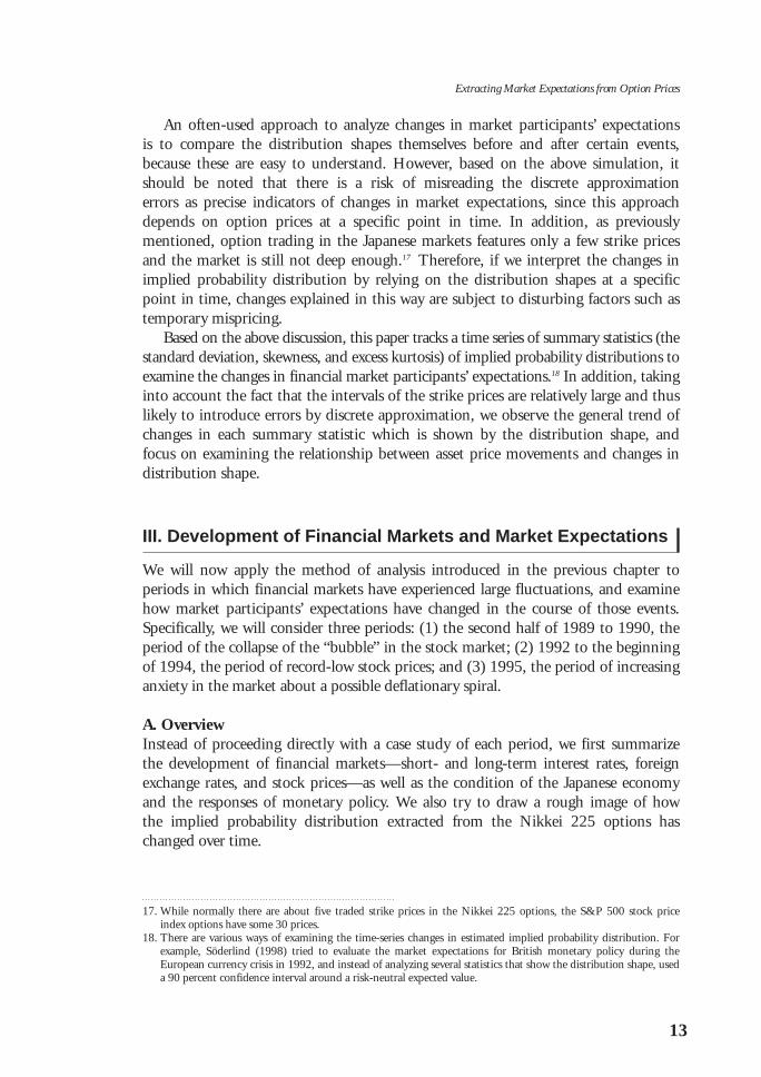
temporarily fell below ¥20,000 in October.23 When we look at the development of stock price expectations during this period (Figure 12), the standard deviation generally rose, and the skewness rose when stock prices fell.

Particularly interesting is the large jump in standard deviation before and after the shiftof the most actively traded contract month during the period from July toSeptember. Specifically, the shift from September options to October options wasdelayed until September 11, three days before the exercise date, and the jump in standarddeviation was quite large. On August 30, owing to the boost in oil prices caused by theIraqi invasion of Kuwait, the official discount rate was raised for the fifth time during the“bubble” era, from 5.25 percent to 6.0 percent, and there seems to have been increasinguncertainty in the market about the future even one month ahead.

Prior to a sharp drop in stock prices from end-September to early October, theskewness rapidly increased from mid- to late September while stock prices declinedmoderately. This implies the possibility that there had been a delay in adjusting stockprice expectations downward, and it is possible to interpret this to mean that, as aresult of bullish sentiment having been largely revised, stock prices fell sharply fromend-September to early October.

Let’s examine how expectations derived from the 10-year JGB futures optiondeveloped during the same period (Figure 13). The standard deviation increasedtoward end-August, when the official discount rate was raised, although it showed a largedrop when the most actively traded contract month shifted. This implies that thetiming of the official discount rate rise was approaching, and the risk of price fluctuationsin the immediate future was quite large. In addition, when declining bond pricesbounced back from end-September (because of the decline in interest rates), the standarddeviation also showed a rapid rise, implying an increasing possibility of price fluctuations.

Distribution att = 1

Distribution att = 2

Persistent confidence on increase

in stock prices

Distribution at t = 0

Strike price

t = 2

Mean of distributionat t = 2

Mean of distributionat t = 0

Mean of distribution at t = 1

t = 1 t = 0

Delays in market expectation adjustment

Figure 11 Market Expectations after Reaching the Historically Highest Price in theStock Markets

Probability density

23. During this period, the Nikkei 225 (closing price) hit bottom at ¥20,221.86 on October 1, although it momen-tarily fell below ¥20,000 and recorded ¥19,781.70 during the trading day.


Figure 12 Market Expectations of the Nikkei 225 (from July to November 1990)


86420

–2–4–6–8

July 1990 Aug. Sep. Oct. Nov.

Percent34,00032,00030,00028,00026,00024,00022,00020,00018,000

Yen


0.350.300.250.200.150.100.05

0


[3] Skewness

2.01.51.00.5

0–0.5–1.0–1.5–2.0


[4] Excess Kurtosis

2.01.51.00.5

0–0.5–1.0–1.5–2.0


Note: Each vertical line with a circle at the top shows the date when the official discount rate was changed (August 30, 1990: 5.25 percent → 6.0 percent), and each vertical dashed line with a diamond at the top shows the date when the most actively traded contract months were changed.

Daily changes (left scale)Stock price level (right scale)

25


Figure 13 Market Expectations of the JGB Futures (from July to November 1990)

[1] JGB Futures

2.52.01.51.00.5

0–0.5–1.0–1.5–2.0–2.5



Futures prices (right scale)

Percent96

94

92

90

88

86

Yen


1086420


[3] Skewness

1.0

0.5

0

–0.5

–1.0July 1990 Aug. Sep. Oct. Nov.

[4] Excess Kurtosis

1.00.5

0–0.5–1.0–1.5–2.0


Note: Each vertical line with a circle at the top shows the date when the official discount rate was changed (August 30, 1990: 5.25 percent → 6.0 percent), and each vertical dashed line with a diamond at the top shows the date when the most actively traded contract months were changed.

Subsequently, the standard deviation declined after the beginning of November. In themeantime, the skewness moved in an opposite direction in accordance with the rise and fall of bond futures prices.

C. The Period of Serious Stock Market SlumpNext, we will examine the period of serious stock market slump, from 1992 to thebeginning of 1994, by dividing the period into two parts: (1) from March to October1992, which includes the point in time when the Nikkei 225 fell below ¥15,000 forthe first time after the collapse of the asset price bubble; and (2) from October 1993to March 1994, when stock prices collapsed again.1. The fall of the Nikkei 225 below ¥15,000 for the first time after the collapse

of the asset price bubble (March–October 1992)First, we examine the movement of market expectations before and after August 18,1992, the day on which the Nikkei 225 fell below ¥15,000 for the first time since theasset price bubble collapsed. Figure 14 shows a time series of summary statistics ofimplied probability distributions.

The standard deviation was on an increasing trend from mid-1991 and hadreached a rather high level by March 1992 (see Figure 8). It further increased whenstock prices tumbled (from late March to early April, in mid-June, and in August),showing that market participants had become increasingly cautious concerning therisk of price changes. Skewness moved in the opposite direction to stock pricechanges, and, on average, increased its level from mid-June to August, implying thatdownward adjustment of stock prices expectations was delayed. Excess kurtosisshowed large fluctuations, which suggests the emergence of large disturbances in thestock market. In particular, from the large fluctuations in late March to early April(when stock prices were falling), and in September (which saw a strong rebound afterthe bottoming out in August), we can observe that expectations became volatile during these periods.24

In the JGB futures market (Figure 15), prices rose (yields fell) from mid-June, andexpectations of a fall in interest rates increased in the market. Prior to the cut in theofficial discount rate in July, the standard deviation declined slightly, while the excesskurtosis, although volatile, increased to around zero. This movement implies thatconfidence in the level of long-term interest rates intensified at that time, and thatthe market had already incorporated a cut in the official discount rate. 2. Another fall in stock prices (October 1993–March 1994)Next, we analyze the period from October 1993 to March 1994, when stock pricesfell again. Figure 16 shows the changes in stock price expectations.

During the period from late October to early December, when stock prices tumbled, the standard deviation increased and the excess kurtosis rose with largeswings, suggesting the increased risk of stock price fluctuations. Skewness alsoincreased, implying that there was a delay in adjusting expectations to the decline in market level.


24. In addition, a jump of standard deviation at the time of contract shift during the stock price bottom can also beinterpreted to show the increase in uncertainty about future stock prices.

27


Figure 14 Market Expectations of the Nikkei 225 (from March to October 1992)


8

6

4

2

0

–2

–4

–6Mar. 1992 Apr. May June July Aug. Sep. Oct.



Percent21,000

20,000

19,000

18,000

17,000

16,000

15,000

14,000

Yen


0.450.400.350.300.250.200.150.100.05

0

Mar. 1992 Apr. May June July Aug. Sep. Oct.

[3] Skewness

2.01.51.00.5

0–0.5–1.0–1.5–2.0–2.5


[4] Excess Kurtosis


Note: Each vertical line with a circle at the top shows the date when the official discount rate waschanged (April 1, 1992: 4.5 percent → 3.75 percent; July 27, 1992: 3.75 percent → 3.25 percent),and each vertical dashed line with a diamond at the top shows the date when the most activelytraded contract months were changed.

543210

–1–2


Figure 15 Market Expectations of the JGB Futures (from March to October 1992)

[1] JGB Futures

2.01.51.00.5

0–0.5–1.0–1.5


Percent107

106

105

104

103

102

101

100

Yen


5

4

3

2

1

0Mar. 1992 Apr. May June July Aug. Sep. Oct.

[3] Skewness

1.0

0.5

0

–0.5

–1.0


[4] Excess Kurtosis

1.00.5

0–0.5–1.0–1.5–2.0


Note: Each vertical line with a circle at the top shows the date when the official discount rate waschanged (April 1, 1992: 4.5 percent → 3.75 percent; July 27, 1992: 3.75 percent → 3.25 percent),and each vertical dashed line with a diamond at the top shows the date when the most activelytraded contract months were changed.



29


Note: Each vertical line with a circle at the top shows the date when the official discount rate waschanged (September 21, 1993: 2.5 percent → 1.75 percent), and each vertical dashed line with adiamond at the top shows the date when the most actively traded contract months were changed.

Figure 16 Market Expectations of the Nikkei 225 (from September 1993 to March 1994)


21,000

20,000

19,000

18,000

17,000

16,000

15,000

14,000

8

6

4

2

0

–2

–4

–6

0.400.350.300.250.200.150.100.05

0

Sep. 1993 Oct. Nov. Dec. Jan. 1994 Feb. Mar.






Percent Yen


[3] Skewness

2.01.51.00.5

0–0.5–1.0–1.5–2.0–2.5

[4] Excess Kurtosis

543210

–1–2

In January 1994, stock prices recovered, although the standard deviation also roserapidly, suggesting an increase in price fluctuation risk. In addition, since there was alarge jump in the standard deviation at the time of changes in the most activelytraded contract months, uncertainty concerning the sustainability of the stock pricerecovery seems to have been strong. In fact, when price recovery came to a halt inFebruary, the standard deviation increased sharply and the excess kurtosis becamehighly volatile, suggesting that the anxiety about the stock price fall had spread in the stock market.

Developments in the JGB futures market are shown in Figure 17. Between lateNovember 1993 and early February 1994, when bond prices rose and yields fell, theskewness remained negative while moving up and down according to changes inbond prices. This implies that downward risk of bond prices was large and confi-dence in price rises was not necessarily strong. Moreover, the standard deviationshowed a distinctive movement, substantially increasing in January 1994 and fallingrapidly in February. At this time, in addition to diminishing expectations of an earlycut in the official discount rate due to the recovery in the stock prices, the concernthat an extra issue of government bonds and the resumption of bond sales by thegovernment might worsen supply and demand conditions in the market seems tohave led to increased expectations of a falling market.

D. Anxiety about a Possible Deflationary SpiralFinally, we will consider the period from December 1994 to September 1995, when the yen appreciated rapidly and anxiety about a possible deflationary spiralintensified. Specifically, we examine the relationship between market expectationsand monetary policy operations for the sub-periods of (1) December 1994 to May1995, when the yen appreciated rapidly; and (2) April to September 1995, when theNikkei 225 temporarily fell below ¥15,000.1. Rapid appreciation of the yen (December 1994–May 1995)First we focus on the period from December 1994 to May 1995. During this period,the yen gradually appreciated from January onward, then accelerated rapidly afterMarch to break the ¥80 level against the U.S. dollar. The stock market was in a declining trend from January onward, and after undergoing alternate phases of sudden and gradual declines, the Nikkei 225 fell close to ¥15,000 early in April.

Figure 18 shows changes in stock price expectations during this phase. During thefirst decline in late January 1995, immediately after the Great Hanshin-AwajiEarthquake,25 all three summary statistics (the standard deviation, skewness, andexcess kurtosis) substantially increased. Subsequently, however, the skewness droppedback to the level prior to the increase in accordance with changes in the most activelytraded contract months, and the increase of the skewness and excess kurtosis disappeared in a relatively short period of time. Therefore, the impact of the stockprice fall seems to have been smoothly absorbed by the market as a temporary shock.


25. The Great Hanshin-Awaji Earthquake was the worst natural disaster in 70 years in Japan. More than 5,000 people died, and an additional two million people, including foreign residents, were significantly affected.

31


Figure 17 Market Expectations of the JGB Futures (from September 1993 to March 1994)

[1] JGB Futures

Percent1.5

1.0

0.5

0

–0.5

–1.0

–1.5

Yen120

118

116

114

112

110

108








10

8

6

4

2

0

[3] Skewness

1.0

0.5

0

–0.5

–1.0

[4] Excess Kurtosis

1.0

0.5

0

–0.5

–1.0

–1.5

–2.0



Figure 18 Market Expectations of the Nikkei 225 (from December 1994 to May 1995)


Percent20,000

19,000

18,000

17,000

16,000

15,000

Yen4

2

0

–2

–4

–6

0.30

0.25

0.20

0.15

0.10

0.05

0






[3] Skewness

1.51.00.5

0–0.5–1.0–1.5

[4] Excess Kurtosis

1.5

1.0

0.5

0

–0.5

–1.0

–1.5

Note: Each vertical line with a circle at the top shows the date when the official discount rate waschanged (April 14, 1995: 1.75 percent → 1.0 percent), and each vertical dashed line with adiamond at the top shows the date when the most actively traded contract months were changed.



In contrast, during the stock price fall from late February to early April, the skewness, while showing volatile movement opposite to the changes in the stockprices, remained consistently positive. The standard deviation increased, and theexcess kurtosis exhibited volatile movements. Such movements in the summary statistics imply that downward adjustments of stock price expectations lagged behind,while the risk of a price fall was increasing.

In the meantime, from late February onward, long-term interest rates declinedand bond prices increased. When we look at the expectation distribution of the JGB futures prices (Figure 19), the standard deviation increased substantially frommid-February to mid-April, while the skewness gradually declined in accordance withthe rise in bond prices. These movements suggest that, from late February onward,market participants started to incorporate expectations of a cut in the official discount rate, which occurred in April.2. The fall of the Nikkei 225 below ¥15,000 (April–September 1995)Next, we take up the period from April to September 1995, when the Nikkei 225 fellbelow ¥15,000. During this period, the yen slowed its pace of appreciation andturned to depreciation from July onward, and the Nikkei 225 fell below ¥15,000twice (in mid-June and from end-June to the beginning of July).

The changes in market expectations during this phase of falling stock prices(Figure 20) were that the skewness increased along with the price fall in mid-Juneand maintained this increased level, while the standard deviation rose. The excesskurtosis exhibited unstable movements, although its swing remained small. Thesemovements in the summary statistics suggest that there was a delayed adjustment to the fall in stock prices, and due to the differing prospects about the effects of theeconomic stimulus package, market expectations seem to have diversified.

In addition, the summary statistics exhibited irregular movements from mid-Julyto September. Unique to this period were the large positive value of the excess kurtosis and the large jump in the standard deviation when the most actively tradedcontract months changed. Such changes imply that, even in the course of stock pricerecovery after July, market participants remained well aware of a downside risk in stock prices.

While a consensus prevailed concerning the economic slowdown that occurredfrom May to July, the JGB futures prices rose and, from mid-July onward, theyturned down, then rose again from mid-August onward. The probability distributionof the JGB futures prices (Figure 21) tells us that, around the turning point of themarket in early July, the standard deviation increased and the excess kurtosis alsoincreased with some volatility, which implies that there was a perceived increase inthe risk of large price fluctuations. In addition, from mid-August to early September,when the official discount rate was raised, the standard deviation rose, which impliesthat market participants were gradually absorbing the forthcoming rate raise.However, there was a large jump in the standard deviation in mid-August, when themost actively traded contract months changed, which suggests that there might havebeen a large shift in market views around this time.

33



Figure 19 Market Expectations of the JGB Futures (from December 1994 to May 1995)

[1] JGB Futures

2.0

1.5

1.0

0.5

0

–0.5

–1.0

–1.5

Percent Yen118

116

114

112

110

108

106








8

6

4

2

0

[3] Skewness

1.0

0.5

0

–0.5

–1.0

–1.5

[4] Excess Kurtosis

1.51.00.5

0–0.5–1.0–1.5

Note: Each vertical line with a circle at the top shows the date when the official discount rate waschanged (April 14, 1995: 1.75 percent → 1.0 percent), and each vertical dashed line with adiamond at the top shows the date when the most actively traded contract months were changed.

35


Figure 20 Market Expectations of the Nikkei 225 (from April to September 1995)


Percent6

4

2

0

–2

–4

Yen19,000

18,000

17,000

16,000

15,000

14,000Apr. 1995 May June July Aug. Sep.

Apr. 1995 May June July Aug. Sep.



0.350.300.250.200.150.100.05

0


[3] Skewness

1.51.00.5

0–0.5–1.0–1.5–2.0–2.5

[4] Excess Kurtosis

6543210

–1–2





Figure 21 Market Expectations of the JGB Futures (from April to September 1995)

[1] JGB Futures

Percent1.0

0.5

0

–0.5

–1.0

–1.5

124

122

120

118

116

114

Yen








8

6

4

2

0

[3] Skewness

1.0

0.5

0

–0.5

–1.0

–1.5

[4] Excess Kurtosis

1.0

0.5

0

–0.5

–1.0

–1.5


IV. Conclusion

In this paper, we have estimated the time series of implied probability distributionsfor the periods of the collapsing “bubble” (1989–90), serious stock market slump(1992–94), and increasing anxiety about a deflationary spiral (1995). Based on theseestimates, we considered (1) how market expectations of future stock prices and long-term interest rates changed; (2) how and when the relationships between suchmarket expectations and economic indicators changed; and (3) how monetary policyimplementation affected such market expectations.

In summary, market participants’ expectations are too diverse and informative to becaptured merely by using a single summary statistic, i.e., the mean, because the samemean value implies different market expectations and policy implications, dependingon the shape of probability distribution of expected outcome. In particular, sincemarket participants’ confidence in stock prices differs substantially depending ontiming, we can expect to capture more market information, both qualitatively andquantitatively, by carefully examining the changes in market participants’ expecta-tions that lie behind stock price fluctuations. The results presented in this paper suggestthat the implied probability distribution extracted from option prices will provideuseful information for the conduct of monetary policy operations.

This paper found typical patterns linking large fluctuations of asset prices and thechanges in the shape of implied probability distribution extracted from option pricesby tracking the time-series movements of summary statistics. It also considered howto interpret such time-series movements in probability distribution as changes inmarket expectations, and discussed possible policy implications. However, studies onhow to make use of the information extracted from option prices in policy judgmentshave only just begun.26 For example, we have dealt with the effects of asset price fluctuations on market expectations, while issues such as the effects of specific patterns of changes in probability distribution on market fluctuations will be worthexamining for analyses of market liquidity and stress situations.

In addition, as Woodford (1994) and Bernanke and Woodford (1997) pointedout in considering the role of asset prices in monetary policy operations, if a centralbank tries to conduct monetary policy based on a certain feedback rule concerningasset prices, bilateral causality will emerge between asset prices and market participants’ expectations concerning future monetary policy, and thus may lead to adestabilization of the economy.

37


26. Methods of extracting expectations concerning future asset prices from option price information have alreadybeen put in practice by many central banks around the world. Implied forward rates are used in most G-7 countries. However, as regards the utilization of option price information, many countries, at most, evaluate thedispersion of expectations concerning future asset prices by using implied volatility estimated by the Black-Scholes formula. Countries that actively utilize risk-neutral implied probability distributions in monetary policyjudgment are still quite limited in number.

APPENDIX 1: METHODOLOGY FOR ESTIMATING IMPLIEDPROBABILITY DISTRIBUTIONS

In this appendix, we examine two types of estimation methods for implied proba-bility distributions: one method is to estimate a probability density function, and theother is to estimate a cumulative distribution function. In this paper, we apply thelatter estimation method.

A. Estimation of Probability Density FunctionsFirst, we explain the method for estimating a probability density function directly.Supposing a risk-neutral market player, the price of a European-type call option (C )is given by

C = exp[–r (T – t )]E [max(0, FT – K )]+∞ (A.1)

= exp[–r (T – t )]∫ w (FT )max(0, FT – K )dFT ,–∞

where FT, K, w (FT ), and r denote the price of an underlying asset on the expirationdate (t =T ) of the option, the strike price of the option, a risk-free interest rate, and aprobability density function for the value FT, respectively.

In option trading, an investor is required to maintain funds in a margin account whenhe or she writes an option. This is because the investor’s broker and the exchangewant to be satisfied that the investor will not default if the option is exercised.Although the size of the required margin depends on circumstances, the margin calculation is repeated every day. When the calculation indicates that a significantly greater margin is required, a margin call will be made. Thus, the pricing formula for a call option (A.1) can be simplified as follows:

+∞

C = ∫ w (FT )max(0, FT – K )dFT . (A.2)–∞

In addition, if we let CK and CKK be the first and second derivatives of the calloption price, then the call option price satisfies the following conditions:

+∞

CK = –∫ w (FT )dFT , (A.3)K

CKK = w (K ). (A.4)

Similarly, if we let P, PK , andCKK be the European-type put option price, and thefirst and second derivatives of the put option price, then we have

+∞

P = ∫ w (FT )max(0, K – FT)dFT , (A.5)–∞

K

PK = ∫ w (FT )dFT , (A.6)–∞

PKK = w (K ). (A.7)


In the practical application of this approach, a problem arises: there are only afinite number of strike prices. This implies that equations (A.3), (A.4), (A.6), and(A.7) do not hold strictly in the observed market prices, because they assume that thevariable C is continuous in K . Thus we apply the second-order finite differencemethod, as Breeden and Litzenberger (1978) proposed, to equation (A.4), and obtainw (Ki ), the probability density function of the strike price Ki as follows:

Ci –1 – 2Ci + Ci +1w (Ki ) ≈ . (A.8)

(Ki +1 – Ki –1)2

If we let p (K *) be the probability density over [Ki – 0.5κ, Ki + 0.5κ], where κ issome positive value, then we have

p (Ki*) ≈ w (Ki )·κ, (A.9)

which yields

Ci –1 – 2Ci + Ci +1p (Ki*) ≈ , (A.10)Ki +1 – Ki –1

where κ = Ki +1 – Ki (i = 1, 2, 3, . . .). This implies that we can estimate the probabilitydensity for a strike price from three call option prices.

Similarly, in the case of a put option, by applying the second-order finite differ-ence method to equation (A.7), we have

Pi +1 – 2Pi + Pi –1p (Ki*) ≈ . (A.11)Ki +1 – Ki –1

However, this approach has a disadvantage: if the range of observable strike pricesis not wide, the sum of the probabilities will be smaller than unity. Moreover, it cannot distinguish how much of the missing probability is attributable to the upperor lower edge of the probability distribution. This suggests the impossibility of estimating the skewness of the distribution of expected asset price changes.

B. Estimation of Cumulative Distribution FunctionsNext, we examine the other approach, which estimates not the probability densityfunction but rather the cumulative distribution function or implied probability distribution from the option prices (Neuhaus [1995]). This approach focuses on the information content of call (put) option premiums that contain payoff probabilities above (below) the respective strike price. In this case, the relative frequency is calculatedas the difference of the cumulative probabilities for the two adjacent strike prices.

In the call option, from equation (A.3), we have

+∞

CK = –∫ w (FT )dFT = –p (FT ≥ K ). (A.12)K

39


This equation implies that the first-order derivative of the call option price contains information on the cumulative distribution function. By applying the first-order finite difference method, we obtain

Ci –1 – Ci +1p (FT ≥ Ki ) ≈ , (A.13)Ki +1 – Ki –1

yielding the probability as

Ci –1 – Ci +1 Ci – Ci +2p (Ki ) = p (FT ≥ Ki ) – p (FT ≥ Ki +1) ≈ – . (A.14)Ki +1 – Ki –1 Ki +2 – Ki

Analogously, from equation (A.6), we have the probability from the put optionprices as

Pi +2 – Pi Pi +1 – Pi –1p (Ki ) = p (FT ≤ Ki +1) – p (FT ≤ Ki ) ≈ – . (A.15)Ki +2 – Ki Ki +1 – Ki –1

Here, we estimate the probability for the class between two adjacent strike prices,although Breeden and Litzenberger (1978) calculate the probability density over theconstant interval around the respective strike price Ki*.

With this estimation method, we can derive the upper part of a probability distribution above the lowest strike price of a call option, and the lower part of aprobability distribution below the highest strike price of a put option. Thus, we caneliminate the missing probability and obtain the complete probability distribution bycombining these two probability distributions. Since the objective of this paper is toestimate the implied probability distribution to examine the development of marketexpectations, we employ not the method of Breeden and Litzenberger (1978) butthat of Neuhaus (1995).

It is often pointed out that ITM options tend to be priced incorrectly. Therefore,we employ the following strategy to estimate a complete probability distribution: we first calculate two probability distributions from the option premium for OTM call and put options separately, then combine these probability distributions to the complete probability distribution.27 In other words, we use the probability distribution derived from OTM put options in the lower range from the ATM strikeprice, and that derived from OTM call options in the upper range.


27. Needless to say, even though they are OTM options, deep-OTM options tend to be priced incorrectly.Therefore, we excluded the observation in estimating the complete probability distribution, if the calculated relative frequency turned negative.

APPENDIX 2: BASIC FRAMEWORK OF OPTION TRADING IN JAPAN

In this appendix, we summarize the basic trading framework of the Nikkei 225option and the JGB futures option (see the Appendix Table for an outline of eachtransaction).

The Nikkei 225 option (a European-type option) began trading in June 1989.The contract months are four consecutive near-term expiration months, and fivestrike prices are set ¥1,000 and ¥500 above and below the strike price closest to thecentral price, which is initially set as the closing price of the Nikkei 225 on the business day before the first day of trading. The last trading day is the business daybefore the second Friday of each expiration month, and the option can be exercisedon the business day following the last trading day.

The JGB futures option (an American-type option) began trading in May 1990.The contract months are the two closest months to March, June, September, and

41


Appendix Table Trading Mechanism of Financial Options in Japan

Date launchedTrading exchangesUnderlying assetsTrading unitContract month

Expiration date

Trading periodStrike prices

Delivery date

Quotation

Daily price limit

Sources: For the Nikkei 225 options, Osaka Securities Exchange (http://www.ose.or.jp); for options on10-year JGB futures, Tokyo Stock Exchange (http://www.tse.or.jp/).

Nikkei 225 optionJune 12, 1989Osaka Securities ExchangeNikkei 225 stock price indexNikkei 225 multiplied by ¥1,000Four consecutive near-term expirationmonths

The business day before the second Fridayof each expiration month

Four monthsFive strike prices are initially opened with¥500 intervals, i.e., 2 OTMs, 1 ATM, and 2 ITMs. Additional strike prices will beavailable according to the movement of theunderlying Nikkei 225 Stock Average.European-type option (the business dayfollowing the last trading day)

¥5 in the case of premiums at or below¥1,000, and ¥10 in the case of premiumsabove ¥1,000±¥1,000 (previous day’s closing price ofNikkei 225 is less than 20,000); ±¥1,500(20,000–less than 30,000); ±¥2,000(30,000–less than 40,000); ±¥2,500(40,000 or more)

JGB futures optionMay 11, 1990Tokyo Stock ExchangeTen-year JGB futuresJGB futures of ¥100 million in face valueTwo months closest to March, June,September, and December (quarterlymonths) plus one or two serial months(non-quarterly months: since November20, 1997)The last business day of the month prior to the delivery month of the underlyingJGB futuresSix monthsSeven strike prices are initially opened with ¥1 intervals, i.e., 3 OTMs, 1 ATM, and 3 ITMs. Additional strike prices will beavailable according to the underlying JGBfutures’ price movement.American-type option (a buyer of an optionmay exercise the option at any time priorto expiration). All in-the-money options at the end of the expiration date will beautomatically exercised, unless otherwiseinstructed.1/100 points per 100 points (¥10,000 percontract)

Two points upward or downward (¥2 million per contract)

December,28 and seven strike prices are set with three ¥1 intervals above and belowthe central price, which is set based on the closing price of the previous business day.The last trading day is the last business day of the month prior to the delivery monthof the underlying JGB futures, and the option can be exercised at any time duringthe six-month trading period.


28. It should be noted that, in addition to the four contract months mentioned above, short-term option trading thatstarts from the 20th of the month prior to the last trading month has taken place since November 20, 1997.

43


Aït-Sahalia, Yacine, and Andrew W. Lo, “Nonparametric Estimation of State-Price Densities Implicit inFinancial Asset Prices,” Journal of Finance, 53 (2), 1998, pp. 499–547.

Bahra, Bhupinder, “Probability Distributions of Future Asset Prices Implied by Option Prices,” Bank ofEngland Quarterly Bulletin, August 1996, pp. 299–311.

———, “Implied Risk-Neutral Probability Density Functions from Option Prices: Theory andApplication,” Bank of England Working Paper Series, No. 66, 1997.

Bates, David S., “The Crash of ’87: Was It Expected? The Evidence from Options Markets,” Journal ofFinance, 46 (3), 1991, pp. 1009–1044.

———, “Dollar Jump Fears, 1984–1992: Distributional Abnormalities Implicit in Currency FuturesOptions,” Journal of International Money and Finance, 15 (1), 1996, pp. 65–93.

———, “Post-’87 Crash Fears in S&P 500 Futures Options,” NBER Working Paper No. 5894,National Bureau of Economic Research, 1997.

Bernanke, Ben S., and Michael Woodford, “Inflation Forecasts and Monetary Policy,” Journal of Money,Credit and Banking, 29 (4), 1997, pp. 654–684.

Black, Fischer, and Myron Scholes, “The Pricing of Options and Corporate Liabilities,” Journal ofPolitical Economy, 81 (3), 1973, pp. 637–659.

Breeden, Douglas T., and Robert H. Litzenberger, “Prices of State-Contingent Claims Implicit inOption Prices,” Journal of Business, 51 (4), 1978, pp. 621–651.

Chen, Ren-Raw, and Louis Scott, “Pricing Interest Rate Futures Options with Futures-StyleMargining,” Journal of Futures Markets, 13 (1), 1993, pp. 15–22.

Cox, John C., and Stephen Ross, “The Valuation of Options for Alternative Stochastic Processes,”Journal of Financial Economics, 3 (1/2), 1976, pp. 145–166.

Hull, John C., Options, Futures, and Other Derivatives, 3rd ed., Prentice-Hall, 1997.Malz, Allan M., “Using Option Prices to Estimate Realignment Probabilities in the European Monetary

System: The Case of Sterling-Mark,” Journal of International Money and Finance, 15 (5), 1996,pp. 717–748.

Melick, Williams R., and Charles P. Thomas, “Recovering an Asset’s Implied PDF from Option Prices:An Application to Crude Oil during the Gulf Crisis,” Journal of Financial and QuantitativeAnalysis, 32 (1), 1997, pp. 91–115a.

Neuhaus, Holger, “The Information Content of Derivatives for Monetary Policy: Implied Volatilitiesand Probabilities,” Discussion Paper 3/95, Economic Research Group of the DeutscheBundesbank, 1995.

Oda, Nobuyuki, and Yoshinao Yoshiba, “Deribatchibu Shohin Kakaku kara Doshutsu Kano na ShijoJoho o Riyo Shita Maaketto Bunseki (Market Analysis Using Market Information Extractedfrom Derivatives Products Prices),” Kin’yu Kenkyu (Monetary and Economic Studies), 17 (2),Institute for Monetary and Economic Studies, Bank of Japan, 1998 (in Japanese).

Söderlind, Paul, “Extracting Expectations about 1992 UK Monetary Policy from Option Prices,” CEPRDiscussion Paper, No. 1823, 1998.

———, and Lars E. O. Svensson, “New Techniques to Extract Market Expectations from FinancialInstruments,” Journal of Monetary Economics, 40 (2), 1997, pp. 383–429.

Woodford, Michael, “Nonstandard Indicators for Monetary Policy: Can Their Usefulness Be Judgedfrom Forecasting Regressions?” in N. Gregory Mankiw, ed. Monetary Policy, University ofChicago Press, 1994, pp. 95–115.

Yoshiba, Yoshinao, “Risuku Ribaasaru Torihiki no Rironteki Gan’i ni Tsuite (Theoretical Implicationof Risk-Reversal Trading),” Kin’yu Kenkyu (Monetary and Economic Studies), 15 (2), Institutefor Monetary and Economic Studies, Bank of Japan, 1996 (in Japanese).

References

Documents

Extracting Market Expectations from Option Prices: Case