Expectations, Real Exchange Rates, and Monetary Policy

Michael B. Devereux Charles Engel

UBC Wisconsin

February 15, 2008

Abstract

Both empirical evidence and theoretical discussion have long emphasized the impact of `news’ on exchange rates. In most exchange rate models, the exchange rate acts as an asset price, and as such responds to news about future returns on assets. But the exchange rate also plays a role in determining the relative price of non-durable goods when nominal goods prices are sticky. In this paper we argue that these two roles may conflict with one another. If news about future asset returns causes movements in current exchange rates, then when nominal prices are slow to adjust, this may cause changes in current relative goods prices that have no efficiency rationale. In this sense, anticipations of future shocks to fundamentals can cause current exchange rate misalignments. Friedman’s (1953) case for unfettered flexible exchange rates is overturned when exchange rates are asset prices. We outline a series of models in which an optimal policy eliminates the effects of news on exchange rates.

We thank participants in seminars at the European Central Bank and the International Monetary Fund. We thank Joong-Shik Kang for research assistance. Engel received support for this research from a grant from the National Science Foundation, Award No. SES -0451671.

Much of analysis of open economy macroeconomics in the past 30 years has been built on the foundation that exchange rates are asset prices and that some goods prices adjust more slowly than asset prices. If this is true, it means that exchange rates wear two hats: They are asset prices that determine the relative price of two monies, but they also are important in determining the relative prices of goods in international markets in the short run. For example, if export prices are sticky in the exporting currency, then nominal exchange rate movements directly change the terms of trade. While of course the literature has recognized this dual role for exchange rate movements, it has not recognized the implication for exchange-rate or monetary policy. Asset prices move primarily in response to news that alters expectations of the future. Most exchange rate movements in the short run reflect changes in expectations about future monetary or real conditions. But future expectations should not be the primary determinant of the relative price of nondurable goods. Those relative prices ought to reflect current levels of demand and supply. So, news that causes nominal exchange rates to jump may have undesirable allocational effects as the news leads to inefficient changes in the relative prices of goods. It may be that controlling exchange rates – dampening their response to news – is an important objective for monetary policy. The misalignment of relative prices is at the heart of the monetary policy analysis in modern macroeconomic models of inflation targeting. Woodford (2003, p. 12-13) explains: “when prices are not constantly adjusted, instability of the general level of prices creates discrepancies between relative prices owing to the absence of perfect synchronization in the adjustment of the prices of different goods. These relative-price distortions lead in turn to an inefficient sectoral allocation of resources, even when the aggregate level of output is correct.” Here, we are focusing misalignments in relative prices when changes in exchange rates are caused by changes in expectations. This distortion would not be present if all goods prices changed flexibly. Then relative prices would not be forced to incorporate these expectations effects, and nominal goods prices would react (efficiently) to news about the future. To help focus the central idea of this paper, it is useful to make a list of things we are not saying: 1. We are not saying that other models of monetary policy in open economies have not modeled exchange rates as asset prices. They have. Our central insight is that monetary policy must react to news that moves exchange rates. In existing models, the only news that hits the market is shocks to current economic variables. By targeting current economic variables in those models, monetary policy does effectively target the news. But in a realistic model, agents have many other sources of information than simply shocks to current macro aggregates. Targeting the aggregates does not achieve the goal of offsetting the influence of news on relative prices. Our model explicitly allows agents to have information about the future that is different than shocks to the current level of macro variables. 2. The problem we have pinpointed is not one of “excess volatility” in asset prices. We do not construct a model in which there is noise or bubbles in asset prices. Instead, we model the exchange rate as the no-bubble solution to a forward-looking difference equation, so it is modeled as an efficient, rational expectations present discounted value of expected future

fundamentals. Indeed, as West (1988) has demonstrated, the more news the market has, the smaller the variance of innovations in the exchange rate. Nonetheless, it is the influence of that news on exchange rates that concerns us. Our intuition is that movements in nominal exchange rates caused by noise or bubbles would also be inefficient, but we purposely put aside that issue for others to study. 3. We are not saying that monetary policy should target all asset prices, such as equity prices. Our intuition is that exchange rates are different. Exchange rates are the only asset price whose movement directly causes a change in the relative price of two non-durables that have fixed nominal prices. That happens because nominal prices of different goods (or the same good sold in different locations) can be sticky in different currencies. Fluctuations in other asset prices cause a change in the price of a durable (e.g., equity prices are the price of capital) relative to the price of a non-durable. At least in some circumstances, that fluctuation is not a concern of monetary policy. As Woodford (2003, p. 13) explains, “Large movements in frequently adjusted prices – and stock prices are among the most flexible – can instead be allowed without raising such concerns, and if allowing them to move makes possible greater stability of the sticky prices, such instability of flexible prices is desirable.” In particular, we do not assume any distortions in asset markets. For example, Bernanke and Gertler (1999, 2001) examine models in which there are credit market frictions (costly monitoring of borrowers) and a non-fundamental component to equity prices. In our models, these frictions do not appear. 4. We are not saying that a policy of fixed nominal exchange rates is optimal. First of all, in response to traditional contemporaneous disturbances (non-news shocks), exchange rate adjustment may be desirable. But even with news shocks alone, our results do not necessarily say that exchange rates should be fixed, but that unanticipated movements in exchange rates should be eliminated. In fact, anticipated movements in exchange rates may play a role in facilitating relative price movements after a news shock. In general, our point is that news shocks can lead to relative price distortions that are translated through exchange rate changes, and these shocks should be a target of policy. In practice, this may mean that monetary policy should include exchange rates in its policy rule. Technically, our model is simple. The central idea is based on the property that efficient relative prices of non-durable goods depend only on current fundamentals, and should not be directly linked to news about future fundamentals. The clearest statement of independence of current allocations on future fundamentals is in Barro and King (1984). They show that in general equilibrium models with time-additive utility and absenting investment, current (efficient) equilibrium allocations are independent of expectations about future fundamentals. This result extends to an open economy where markets are sufficiently complete to support a time-invariant risk sharing rule. But, in the presence of sticky nominal prices, this dichotomy between current allocations and future fundamentals no longer necessarily holds. When prices cannot adjust, any news shocks that affect the current exchange rate automatically affect relative prices. In general this is inefficient, and the monetary authority should take action to dampen or eliminate the impact of news shocks on current allocations.

3

In section 1, we develop a flexible-price monetary model that illustrates the Barro-King thesis in an open economy with complete markets. In section 2, we proceed to develop a model of forward-looking real exchange rates under sticky nominal prices, and investigate the implications for monetary policy. Our starting point is a model based closely on the one in the important paper of Clarida, Gali, and Gertler (2002). In that model, when nominal prices adjust sufficiently slowly, real exchange rates respond strongly to news about future fundamentals. But that model also illustrates an important principle: under inflation targeting, the effect of news on real exchange rates can be greatly diminished. Indeed, in this model, strict inflation targeting completely eliminates the effects of news on real exchange rates. The Clarida-Gali-Gertler (hereinafter referred to as CGG) model has some special features that drive this stark result. We consider the conclusion unrealistic, if for no other reason than casual empirical observation. Many countries have successfully adopted inflation targeting in recent years – Canada, Australia, New Zealand, the United Kingdom, to name a few – but in all cases it appears that real exchange rates are still quite sensitive to news. At the end of section 2, we delineate these special features of the CGG model that need to be abandoned to build a more plausible open-economy model. Two in particular are germane to our point about the news. First, CGG’s assumption on the inflation process implies that exchange rate movements do not directly influence inflationary pressure. Second, we argue that asset markets respond to news more quickly than goods markets, in contrast to CGG’s assumption. Section 3 then explores a simple model very much like CGG’s but with a different assumption about international price setting. In particular, CGG assume that firms that sell in domestic and foreign markets set a single price for both markets. Instead, we follow Betts and Devereux (1996) and Benigno (2004), for example, and allow firms to set different prices for sale at home and abroad. Crucially, export prices are set in the buyer’s currency. That is, we assume local-currency pricing (LCP). The significance of this assumption is the following: Under CGG’s price setting assumption (producer currency pricing, or PCP), monetary policy can eliminate all of the distortions from nominal price stickiness by driving inflation to zero. Under LCP, however, eliminating inflationary pressure does not eradicate the distortions introduced by sticky prices. Under a pure inflation targeting regime, the real exchange rate is still forward looking in equilibrium, and policies that appropriately target real exchange rate distortions can be desirable. Section 4 then returns to the CGG model, but allows for news to influence asset markets – the foreign exchange market, specifically – more quickly than firms incorporate news into goods prices. We show that with this one modification, inflation targeting could actually exacerbate the distortionary effects of news. Policy that targets real exchange rate misalignments might be appropriate. In section 5, we assess the gains from exchange rate targeting in a model with LCP and this information structure. Our purpose is to get a “back of the envelope” assessment of the gains from adding an exchange-rate target to the monetary rule in an open economy. This exercise is not intended to build a “realistic” model of the open economy, such as the models that are used by many central banks, but to investigate whether this avenue for potential future research is likely to be fruitful. In other words, when foreign exchange markets incorporate

4

news about the future, are there channels through which foreign exchange rate fluctuations are distortionary in a quantitatively important way? And, are there potential gains from policymakers targeting exchange rates? Our evidence suggests the answer to these questions is yes. In our analysis of two-country models of the global economy, we shall only consider cooperative monetary policies. That is, we consider policies that maximize the sum of welfare in our two symmetric countries. This simplifies the analysis, but abstracts from any issues of whether central banks will be tempted to undertake competitive devaluations, for example.1 We also only consider monetary policy under commitment. While interesting issues arise when policymakers cannot commit, our sense is that – as in CGG, which analyzes both cases – the basic nature of optimal policy rules in the settings we consider is not very different in the two cases. Also, in our numerical simulations of section 5, we consider only easily implementable and observable policy rules, rather than searching for the optimal set of targets in the policy rule. Section 2. The Flexible Price Model

The insight that news about future fundamentals should not affect the equilibrium in a dynamic general equilibrium models under complete markets was first discussed by Barro and King (1984). In a closed economy model with time-additive utility and without endogenous investment, they show that all real allocations and relative prices are determined solely by contemporaneous fundamentals. That is, there are no intrinsic inter-temporal links between periods, and no persistence in the effects of shocks, apart from that due to persistence in the shocks themselves. An equilibrium allocation in their model is Pareto efficient, since there is a representative individual and all prices are fully flexible. It follows that, in an economy with sticky prices, if an optimal monetary policy is designed to replicate the flexible price equilibrium, it should insulate current allocations and relative prices against shocks that come in the form of announcements about future fundamentals. We further develop this basic intuition within the standard two-country environment of recent open economy macroeconomic models. Although the analytical results rely on the strict separation across periods, we do not argue that it be taken literally. There are a number of factors that give rise to efficient links between current allocations or relative prices and future fundamentals shocks. One obvious channel is investment. But we argue that even once we allow for this linkage, our central result – that the current exchange rate response to announcements about future fundamentals should be dampened – will still hold in a quantitative sense. There are two countries, each with a population normalized to one. Each country produces a nontraded final good using traded intermediate goods. The final good is sold in competitive markets. Each final good is produced using a continuum of intermediate goods produced in the home country and a continuum of intermediate goods produced in the foreign

1 Analysis of the non-cooperative case can be very difficult, even under complete markets. Many studies that investigate non-cooperative policy take initial wealth as exogenous, but this approach sidesteps the tricky issue that policy rules can influence the distribution of wealth. (See, for example, Devereux and Engel, 2003.) We also note that the analysis of cooperative policies can be complicated when markets are incomplete, because the objective function of the policymaker might incorporate time-varying weights as the wealth distribution shifts. That issue does not arise for us here because we assume complete markets.

5

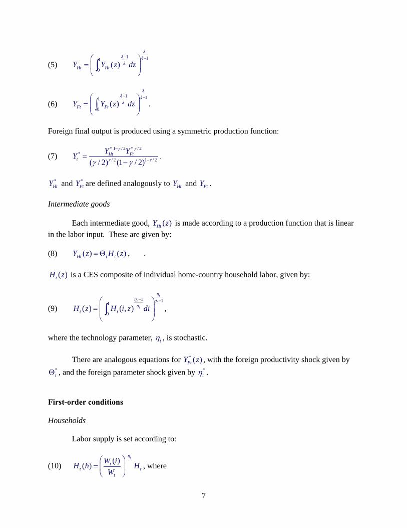
country. Production of the final good in each country exhibits home bias. Intermediate goods are produced in an imperfectly competitive environment. Shocks to the model come from productivity, to the elasticity of demand by final goods firms for services of intermediate goods firms, and later on, liquidity shocks affecting nominal interest rates. This model corresponds closely to the CGG model, except that we add the assumption of home bias in the demand for intermediate goods used in the production of final consumer goods. Households

The representative household in the home country maximizes

(1) 1 1

0

1( ) ( ) ( )1 1

jt t t j t j

jU i E C i H iρ ζβ

ρ ζ

∞− +

+ +=

⎧ ⎫⎡ ⎤= −⎨ ⎬⎢ ⎥− +⎣ ⎦⎩ ⎭

∑

( )tC i is consumption of the final good produced in the home country. is an aggregate of

the labor services that the household sells to each of a continuum of intermediate firms located in the home country:

( )tH i

(2) . 1

0( ) ( , )t tH i H i z dz= ∫

Households receive wage income, , aggregate profits from home firms, ( )t tW H i tΠ , and can trade in a complete market in contingent claims (arbitrarily) denominated in the home currency: (3) . 1 1( ) ( | ) ( , ) ( ) ( ) ( , )

tt

t t t tt t t t t

s

PC i Q s s B i s W i H i B i s+ +

∈Ω

+ = +Π∑ +

Foreign households have analogous preferences and face an analogous budget constraint. Firms Final goods

In the home country, the final consumption good is produced in competitive markets (with freely-set prices) by firms that use a production technology that combines home-produced and foreign-produced intermediate goods:

(4) / 2 1 / 2

/ 2 1 / 2( / 2) (1 / 2)Ht Ft

tY YY

γ γ

γ γγ γ

−

−=−

.

We assume 1 2γ≤ ≤ . There is home bias if 1γ > .

HtY ( ) is a CES aggregate over a continuum of home- (foreign-) produced intermediate goods: FtY

6

(5) 1 11

0( )Ht HtY Y z dz

λλ λλ− −⎛ ⎞

= ⎜ ⎟⎝ ⎠∫

(6) 1 11

0( )Ft FtY Y z dz

λλ λλ− −⎛ ⎞

= ⎜ ⎟⎝ ⎠∫ .

Foreign final output is produced using a symmetric production function:

(7) * 1 / 2 * / 2

*/ 2 1 / 2( / 2) (1 / 2)

Ht Ftt

Y YYγ γ

γ γγ γ

−

−=−

.

*

HtY and are defined analogously to *FtY HtY and . FtY

Intermediate goods Each intermediate good, is made according to a production function that is linear in the labor input. These are given by:

( )HtY z

(8) , . ( ) ( )Ht t tY z H z= Θ

( )tH z is a CES composite of individual home-country household labor, given by:

(9) 1 11

0( ) ( , )

tt t

tt tH z H i z di

ηη ηη− −⎛ ⎞

= ⎜ ⎟⎜ ⎟⎝ ⎠∫ ,

where the technology parameter, tη , is stochastic. There are analogous equations for , with the foreign productivity shock given by

, and the foreign parameter shock given by

* ( )FtY z*t

*tΘ η .

First-order conditions Households Labor supply is set according to:

(10) ( )( )t

tt t

t

W iH h HW

η−⎛ ⎞

= ⎜ ⎟⎝ ⎠

, where

7

(11) ( )1

1 11

0( ) tt

t tW W i di ηη −−= ∫ .

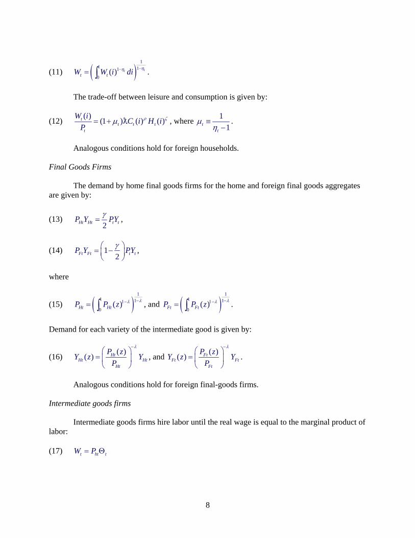
The trade-off between leisure and consumption is given by:

(12) ( ) (1 ) ( ) ( )tt t t

t

W i C i H iP

ρ ζμ= + , where 11t

t

μη

≡−

.

Analogous conditions hold for foreign households. Final Goods Firms The demand by home final goods firms for the home and foreign final goods aggregates are given by:

(13) 2Ht Ht t tP Y PYγ

= ,

(14) 12Ft Ft t tP Y PYγ⎛ ⎞= −⎜ ⎟

⎝ ⎠,

where

(15) ( )1

1 1

0( )Ht HtP P z λλ −1−= ∫ , and ( )

11 1

0( )Ft FtP P z λλ −1−= ∫ .

Demand for each variety of the intermediate good is given by:

(16) ( )( ) HtHt Ht

Ht

P zY z YP

λ−⎛ ⎞

= ⎜ ⎟⎝ ⎠

, and ( )( ) FtFt Ft

Ft

P zY z YP

λ−⎛ ⎞

= ⎜ ⎟⎝ ⎠

.

Analogous conditions hold for foreign final-goods firms. Intermediate goods firms Intermediate goods firms hire labor until the real wage is equal to the marginal product of labor: (17) t htW P= Θt

8

Equilibrium Conditions Because all households are identical, ( )t tW i W= , ( )tL i Lt= , and . ( )t tC i C= Goods market clearing requires: (18) , and . *

t t Ht HtL Y YΘ = + * * *t t Ft FtL Y YΘ = +

Under complete markets, we have the equilibrium condition: (19) * *

t t t t tPC S P Cρ ρ= , where is the nominal exchange rate, expressed as the home currency price of foreign currency.

tS

We define the terms of trade in each country as the price of imports relative to exports in that country:

(20) Ftt

Ht

PP

Τ ≡ , and *

**

Htt

Ft

PP

Τ ≡ .

Log-linearized equilibrium Under the assumption that all households in the home country are identical, we can write the log-linearized first-order condition (12) for households as: (21) t t t tw p c h tρ ζ μ− = + + . The analogous foreign condition is: (22) * * * *

t t t tw p c h *tρ ζ μ− = + + .

The market clearing condition in the home country (18) can be written as:

(23) * *1 12 2 2 2t t t t t th c cγ γ γ γθ τ τ⎛ ⎞⎛ ⎞ ⎛ ⎞⎛+ = + − + − −⎜ ⎟ ⎜ ⎟⎜⎜ ⎟⎝ ⎠ ⎝ ⎠⎝⎝ ⎠

⎞⎟⎠

,

where we have used (13) and (14). In the foreign country,

(24) * * * *1 12 2 2t t t t t th c cγ γ γ

2γθ τ τ⎛ ⎞⎛ ⎞ ⎛ ⎞⎛+ = + − + − −⎜ ⎟ ⎜ ⎟⎜⎜ ⎟⎝ ⎠ ⎝ ⎠⎝⎝ ⎠

⎞⎟⎠

.

9

Given that the optimal mark-ups are the same in the home and foreign country, under flexible prices the law of one price holds for both goods ( *

ht t htp s p= + and *ft t ftp s p= + ). This

implies: (25) *

t tτ τ= − . The equilibrium condition under complete markets, (19), gives us: (25) * *

t t t tc p s c pρ ρ+ = + + t

t

From the cost functions, we derive the relation between the real exchange rate and the terms of trade: (26) * ( 1)t t t tq s p p γ τ≡ + − = − . From intermediate firms’ optimization, (17), we find: (27) t htw p tθ− = and * *

t ftw p *tθ− = .

We can solve this model without considering any dynamic first-order conditions or expectations of the future. This is an example of the Barro-King theorem, applied to an open economy. We use the notation *ˆt t tx x x= − to denote home relative to foreign values. From the first-order conditions for households and firms (labor supply and labor demand), we derive an expression for the terms of trade: (28) ˆˆ ˆt t th tτ θ ζ μ= − − . The home relative to the foreign market clearing condition can be written as:

(29) 1ˆ ˆ (2 )t t th q tγ θ γ γρ−

= − + − τ

t

.

Noting that *

tτ τ= − and ( 1)tq tγ τ= − , we can solve these two equations to get an expression for

the terms of trade tτ in terms of tθ and ˆtμ :

(30) 2 2

(1 ) ˆ ˆ(( 1) (2 )) (( 1) (2 ))t t t

ρ ζ ρτ θ μρ ζ γ ργ γ ρ ζ γ ργ γ

+= −

+ − + − + − + −.

With this solution, we can readily solve for the equilibrium values of other key variables such as consumption and employment. We can write,

10

( )1 1( 1)t t th tρ γ τ θ μρ ζ ρ ζ−

= − − −+ +

.

Substituting the expression for tτ from equation (30) into this expression yields a solution for in terms of

th

tθ , *tθ , tμ , and *

tμ . Equilibrium consumption, c , can be expressed in terms of the same four current period fundamentals by substituting the solutions for and

t

th tτ into this relationship:

1 1( 1 )2t t t tc hγ ζ

tθ τ μρ ρ ρ

⎛ ⎞= − − − −⎜ ⎟⎝ ⎠

.

The important point to emphasize is that the equilibrium values for the real exchange rate, the terms of trade, consumption, employment and other real variables under flexible prices (and complete markets) depend only on current levels of productivity, tθ and *

tθ , and mark-ups,

tμ and *tμ . News of future productivity or mark-up shifts has no influence on these equilibrium

relative prices. We now explore the implication of this result in a number of settings where prices are

sticky.

2. Sticky Prices – PCP case We first consider the case of producer currency pricing. Intermediate firms in each country set only one price, whether the good is sold in the home or foreign country. Home firms set htp in home currency, and *

ht ht tp p s= − . Foreign firms set *ftp in foreign currency, and

*ft tp s ftp= + . In the next section, we consider local currency pricing, where each firm sets a

home-currency price for sale in the home country and a foreign currency price for sale in the foreign country. We consider LCP to be more realistic than PCP. While the data for advanced countries do not match either assumption perfectly, there are gross violations of the law of one price, and relative prices of goods closely mimic the nominal exchange rate (as under LCP). We pursue the PCP model here because it generates a reduced-form model that is isomorphic to the canonical closed-economy model. This is helpful for expositional purposes. As shown in the Appendix, under PCP, the open-economy Phillips curves take on the familiar forms: (31) 1( )Ht t Ht t t Htw p Eπ κ θ β π += − − + (32) * * * *

1( )Ft t Ft t t Ftw p E *π κ θ β π += − − + . where we use the notation π everywhere to denote inflation, the first-difference in the log of the price (so, for example, 1Ht Ht Htp pπ −≡ − .)

11

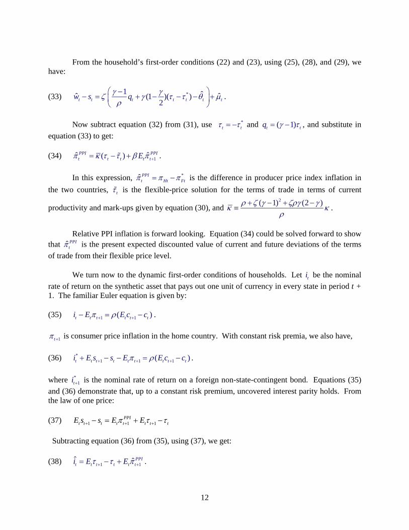
From the household’s first-order conditions (22) and (23), using (25), (28), and (29), we have:

(33) *1 ˆˆ ˆ(1 )( )2t t t t t tw s qγ γ

tζ γ τ τ θρ

⎛ ⎞−− = + − − − +⎜ ⎟

⎝ ⎠μ

t

.

Now subtract equation (32) from (31), use *

tτ τ= − and ( 1)tq tγ τ= − , and substitute in equation (33) to get: (34) 1ˆ ˆ( )PPI PPI

t t t tE tπ κ τ τ β π += − + . In this expression, *ˆ PPI

t Ht Ftπ π π= − is the difference in producer price index inflation in the two countries, tτ is the flexible-price solution for the terms of trade in terms of current

productivity and mark-ups given by equation (30), and 2( 1) (2 )ρ ζ γ ζργ γκ κρ

+ − + −≡ .

Relative PPI inflation is forward looking. Equation (34) could be solved forward to show that ˆ PPI

tπ is the present expected discounted value of current and future deviations of the terms of trade from their flexible price level. We turn now to the dynamic first-order conditions of households. Let be the nominal rate of return on the synthetic asset that pays out one unit of currency in every state in period t + 1. The familiar Euler equation is given by:

ti

(35) 1 1( )t t t t t ti E E c cπ ρ+ +− = − .

1tπ + is consumer price inflation in the home country. With constant risk premia, we also have, (36) . *

1 1 1( )t t t t t t t t ti E s s E E c cπ ρ+ + ++ − − = − where is the nominal rate of return on a foreign non-state-contingent bond. Equations (35) and (36) demonstrate that, up to a constant risk premium, uncovered interest parity holds. From the law of one price:

*1ti +

(37) 1 1

PPIt t t t t t t tE s s E E 1π τ τ+ + +− = + −

Subtracting equation (36) from (35), using (37), we get: (38) 1 1

ˆ ˆ PPIt t t t t ti E Eτ τ π+ += − + .

12

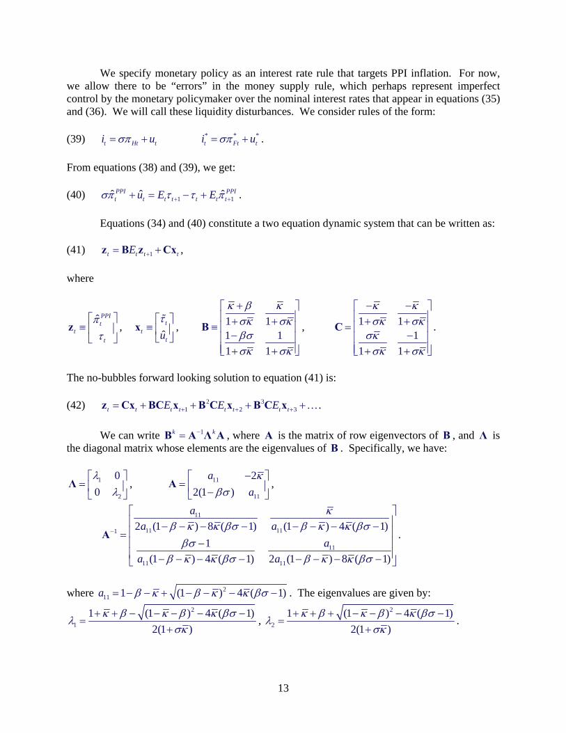
We specify monetary policy as an interest rate rule that targets PPI inflation. For now, we allow there to be “errors” in the money supply rule, which perhaps represent imperfect control by the monetary policymaker over the nominal interest rates that appear in equations (35) and (36). We will call these liquidity disturbances. We consider rules of the form: (39) t Hti utσπ= + . * *

t Fti uσπ= + *t

From equations (38) and (39), we get: (40) 1 1ˆ ˆ ˆPPI PPI

t t t t t t tu E Eσπ τ τ+ ++ = − + π

t

. Equations (34) and (40) constitute a two equation dynamic system that can be written as: (41) , 1t t tE += +z B z Cx where

ˆ PPIt

tt

πτ

⎡ ⎤≡ ⎢ ⎥⎣ ⎦

z , ˆ

tt

tuτ⎡ ⎤

≡ ⎢ ⎥⎣ ⎦

x , 1 11 11 1

κ β κσκ σκβσσκ σκ

+⎡ ⎤⎢ ⎥+ +≡ ⎢ ⎥−⎢ ⎥

⎢ ⎥+ +⎣ ⎦

B , 1 11

1 1

κ κσκ σκ

σκσκ σκ

− −⎡ ⎤⎢ ⎥+ += ⎢ ⎥

−⎢ ⎥⎢ ⎥+ +⎣ ⎦

C .

The no-bubbles forward looking solution to equation (41) is: (42) . 2 3

1 2 3t t t t t t t tE E E+ + += + + + +z Cx BC x B C x B C x … We can write , where A is the matrix of row eigenvectors of , and is the diagonal matrix whose elements are the eigenvalues of . Specifically, we have:

1k −=B A Λ Ak B ΛB

1

2

00λ

λ⎡ ⎤

= ⎢ ⎥⎣ ⎦

Λ , 11

11

22(1 )

aaκ

βσ−⎡ ⎤

= ⎢ ⎥−⎣ ⎦A ,

11

11 111− =A11

11 11

2 (1 ) 8 ( 1) (1 ) 4 ( 1)1

(1 ) 4 ( 1) 2 (1 ) 8 ( 1)

aa a

aa a

κβ κ κ βσ β κ κ βσβσ

β κ κ βσ β κ κ βσ

⎡ ⎤⎢ ⎥− − − − − − − −⎢ ⎥

−⎢ ⎥⎢ ⎥− − − − − − − −⎣ ⎦

.

where 2

11 1 (1 ) 4 (a β κ β κ κ βσ= − − + − − − −1) . The eigenvalues are given by: 2

11 (1 ) 4 ( 1)

2(1 )κ β κ β κ βσ

λσκ

+ + − − − − −=

+,

2

21 (1 ) 4 (

2(1 )κ β κ β κ βσ

λσκ

1)+ + + − − − −=

+.

13

Equation (42) demonstrates that relative PPI inflation, ˆ PPItπ , and the terms of trade, tτ are

forward looking variables that depend on the current and expected future values of tτ and the exogenous relative liquidity variable, . In turn, ˆtu tτ is a linear function of the relative

productivity level, tθ , and relative mark-ups, ˆtμ . Specifically, ˆ PPItπ and tτ are each sums of

two present discounted value sums, with discount factors given by 1λ and 2λ . These variables

are more “forward looking” – that is, the weight on future expected values of , ˆtu tθ , and ˆtμ -- the closer are 1λ and 2λ to unity. As inflation responds less to current excess demand, so 0κ → , we find 1 1λ → and

2λ β→ . That is, the expected value of the future states will matter a lot for the current level of the terms of trade when prices are very sticky. This starkly contrasts with the flexible price model in which tτ depends only on current values of tθ and ˆtμ . Since under PCP we still have

(tq 1) tγ τ= − , the same statements apply to the real exchange rate. Holding κ constant, suppose the monetary authorities followed strict inflation targeting so σ →∞ . Then 1 0λ → and 2 0λ → . This means the discount factors in the discounted sum (42) go to zero. Under strict inflation targeting, expectations of the future state do not affect the equilibrium terms of trade. Indeed, that can be seen directly from equation (34): if in every date the monetary policymaker succeeds in driving Htπ to zero, then we must have t tτ τ= . In order for inflation to be zero, the terms of trade must equal their flexible price value. In the absence of mark-up shocks, so ˆ 0tμ = , and liquidity shocks, so u , the policy rule of letting

ˆ 0t =σ →∞ is optimal. It reproduces the flexible price equilibrium, which is efficient

(assuming the optimal constant subsidy rates are in place to eliminate the monopoly distortions in wage setting and price setting.) The logic is straightforward. In this case, the only distortion to the economy comes from nominal price stickiness. If policymakers can succeed in holding nominal producer prices constant, then firms have no incentive to change their optimal nominal price. Nominal price stickiness is rendered moot. This system closely adheres to the model of Clarida, Gali, and Gertler (2001), and is the well-known case in which the open economy model is “isomorphic” to the closed-economy model. That is, the dynamic system (42) holds for the closed economy analogy to this open economy model. Simply replace relative PPI inflation with Htπ , and replace the terms of trade with GDP, and we have a system that is analogous to the canonical closed-economy system. Because of our assumption of complete markets, the terms of trade are proportional to relative

consumption: ˆ1t ct

ρτγ

=−

. With minor adjustments to coefficients, under PCP we can take a

closed economy model expressed in terms of domestic inflation Htπ and domestic output (which equals domestic consumption, , when there is no investment or government spending), and convert it into a model of relative inflation,

tcˆ PPI

tπ , and the terms of trade, tτ .

14

We know that targeting both inflation and the output gap in the closed-economy version of this model is superior to targeting inflation alone. That is, because of the time-varying mark-ups (and, in our model, liquidity disturbances), optimal policy does not completely drive inflation to zero. In the open economy model, by analogy, policy that targets tτ will improve on a pure inflation-targeting strategy. If σ takes on relatively small values (but greater than unity), and κ is small, then the real exchange rate puts heavy weight on expectations of the future. A policy that targets deviations of tτ from the value it would attain under a competitive flexible-price economy may be welfare improving. Ideally, we want the terms of trade to be able to respond to current productivity levels. But when the discount factor is high, tτ puts high weight on expectations of the future. Most of the variance of the terms of trade is determined by expected future values of , ˆtu tθ , and ˆtμ . An extreme policy that completely stabilizes tτ has the deleterious effect of eliminating the response of the terms of trade to current productivity shocks, but this must be weighed against the distortionary effects of having tτ respond to news about future shocks that is unrelated to the current productivity levels. It is instructive to consider the following example. Suppose 1σβ = . That case is admissible – the coefficient on inflation in the Taylor rule is greater than one. But with only mild inflation targeting, the discount factors in the present value relationships in equation (42)

are large: 1 1βλβ

=−

, and 2βλ

κ β=

+.

Suppose further that tτ and each follow AR(1) stochastic processes: ˆtu 1t t tτ ττ δ τ ε−= + ,

and 1ˆ ˆt u tu u utδ ε−= + , where 1 ,τ 1uδ δ− ≤ ≤ . At time t, agents receive some news about 1tτε + and

1utε + , but not about shocks in any future period so that 1j

t t j t tE Eττ δ τ+ += and for . Then we can solve to find:

1ˆ ˆjj u t tE uδ+ +=t tE u

0j ≥

1 1ˆ(1 ) (1 )t t t t t

u

u Eτ

κ β β κ β βτ τ τβ κ β κ δ β κ β κ δ β κ β κ

ˆt tE u+ +

⎛ ⎞ ⎛= − + −⎜ ⎟ ⎜+ + − + + − + +⎝ ⎠ ⎝

⎞⎟⎠

.

When inflation is not very responsive to the deviations of the terms of trade from their flexible-price level, so κ is low (relative to β ), the expected future fundamentals receive a high weight relative to current fundamentals in determining the terms of trade.

Alternatively, we can write the solution in terms of the current levels of the fundamentals and the news about the future:

1 1

ˆ(1 ) (1 )

(1 ) (1 )

t t tu

t t t utu

u

E E

τ

ττ

κ βτ τδ β κ δ β κ

κ β β βε εδ β κ β κ δ β κ β κ+ +

= −− + − +

⎛ ⎞ ⎛+ −⎜ ⎟ ⎜− + + − + +⎝ ⎠ ⎝

⎞⎟⎠

.

15

This equation shows the forces influencing the deviation of the terms of trade from its flexible-price value. When κ is small relative to β , the news about future fundamentals receives almost as much weight as the current fundamentals in determining the level of the terms of trade. An informative special case is when the log of productivity and mark-ups follow a pure random walk, 1τδ = , and there are no liquidity disturbances, u 0t = . If agents receive no news about future shocks, then the economy attains the flexible-price equilibrium ( t tτ τ= ). This attains even though monetary policy does not follow strict inflation targeting. (We have assumed 1σβ = , but in fact under the assumption of 1τδ = and ˆtu 0= , we obtain the result that

t tτ τ= for any value of 1σ > .) Intuitively, in this environment, in equilibrium price setters face a stationary environment and therefore have no incentive to change nominal prices. However, when there is news about the future ( 1 0t tE τε + ≠ ), the flexible-price equilibrium is not attained. The environment facing price-setting firms is no longer stationary, and distortionary price changes occur. All of the distortion in this economy is due to news about the future. As we have noted above, by analogy to CGG, in the model with mark-up disturbances strict inflation targeting (σ →∞ ) is not optimal. When σ is not too large, the real exchange rate still responds to news, so the “news” distortion is not eliminated. But we do not believe this model makes a strong case for targeting real exchange rate misalignments. In fact, CGG argue in favor of a policy rule that targets the output gap and the inflation gap. As subsequent literature has emphasized (see, for example, Blanchard and Gali (2007)), introducing mark-up variation is essentially a gimmick to introduce a role for output gap stabilization into the monetary rule. Sticky nominal wages (see Erceg, Henderson, and Levin (2001)) provide another reason why monetary policymakers may want to target the output gap. From this point forward, we will drop the mark-up disturbances and liquidity disturbances, thus eliminating any role for output gap stabilization. We will correspondingly not consider policy rules that include the output gap. In the model we have examined so far, then, strict inflation targeting is optimal (when the optimal subsidy to monopolists is in place to eliminate the static monopoly distortion.) But we now list four features of open economies that make them different from closed economies – features which break the isomorphism between closed and open economy models: 1. We have emphasized the asset price nature of the real exchange rate – that it is forward looking and might depend heavily upon news about the future. But in the isomorphic closed-economy model, the same can be said about consumption. However, this aspect of the canonical model has generated scrutiny, because actual consumption does not seem so forward looking. One proposed solution is to introduce habit persistence. In general, equation (35) could be written as: 1 1( ) (t t t t t ti E E mu c mu c )π + +− = − + .

16

Marginal utility is forward looking. This equation can be solved forward to write marginal utility at time t as the undiscounted sum of current and expected future real interest rates. But even if marginal utility is purely forward looking, under habit persistence, actual consumption will have a backward looking element. Marginal utility at time t depends on lagged consumption. However, under complete markets, the real exchange rate is related to marginal utilities, not consumption levels: . *( ) ( )t tq mu c mu c= − + t

1))+

tc

The real exchange rate is forward looking even under habit persistence. That is, * *

1 1( (t t t t t t t t tq E q i E i Eπ π+ += − − − − so the real exchange rate is the undiscounted sum of current and expected future relative CPI real interest rates. In the closed economy, it is the marginal utility – the pricing kernel for real payoffs – that is forward looking. That does not mean, however, that the closed economy model is isomorphic to the open economy, with the pricing kernel mapping into the real exchange rate. In the closed economy, demand depends on the actual consumption level, which is less sensitive to news about the future than the pricing kernel. So inflation is less sensitive to the news under habit persistence. In the open economy, demand for output depends in part on consumption levels, but it also depends in part directly on the real exchange rate. The asset price – the real exchange rate – directly affects demand and inflation. 2. Because ˆtq ρ= under complete markets, if each country were to push its consumption level toward the flexible-price equilibrium value, it would achieve the same goal as targeting the real exchange rate. However, a model that assumes complete markets is not realistic. The relationship that implies proportionality between the real exchange rate and relative consumption is grossly violated in the data. That is, the well-known “Backus-Smith puzzle” or “consumption – real exchange rate anomaly” refers to the empirical finding that the correlation between and

is not high and perhaps generally negative among pairs of OECD countries. While it is standard in closed-economy models to assume individual consumption risk can be fully shared by agents within a country, the assumption of complete markets across countries is not so tenable.

tq

tc

We do not pursue these first two ways in which the isomorphism between closed and open economies will be broken. Instead we focus on the next two, which are salient given our focus on the role of the news. 3. Strict inflation targeting in both countries removes all of the sticky-price distortions under PCP because in that world, there are only two nominal prices – the home-currency price of home goods and the foreign-currency price of foreign-currency goods. The law of one price holds across countries for both goods. When aggregate excess demand for home goods is annihilated by pushing inflation in that price to zero, the sticky-price distortion in the market for home-produced goods is eliminated. Similarly, the foreign price distortion is removed when foreign PPI inflation is driven to zero.

17

There are many cases, however, in which targeting the overall level of demand does not eliminate all distortions. It is these cases that are generally the object of study in international economics (though not so generally in New Keynesian studies of monetary policy in open economies.) For example, if there are shocks that require reallocation of resources between the traded and nontraded sector, but nominal traded and nontraded prices are both sticky, then inflation targeting alone does not remove the distortions related to intersectoral misallocation of resources. We focus on a different but not dissimilar case. Under local-currency pricing, the prices of imported goods relative to exported goods – that is, the terms of trade – cannot adjust optimally to productivity shocks even under inflation targeting. For example, CPI inflation targeting will drive aggregate excess demand toward zero, but relative prices do not adjust optimally. As we will explain in the next section, under LCP there are distortions coming from the failure of the law of one price (the same good sells for different prices at home and abroad), and the terms of trade do not adjust optimally to changes in productivity in each country. Even under strict inflation targeting, the real exchange rate will incorporate news about future productivity disturbances and relative prices will be distorted from their efficient levels. 4. Financial markets incorporate news quickly into asset prices. Goods markets to not appear to incorporate news as quickly into goods prices. Perhaps this is a reflection of the difference in the products sold in the two markets: Foreign exchange markets sell a homogenous asset in deep markets that is costlessly transportable. Goods markets sell differentiated products that are costly to transport in thin markets. Zbaracki et. al. (2004) document the actual time-consuming process in a case study of a large U.S. manufacturing firm. Changing prices is a process that consumes several months. One of the chief costs of setting prices is gathering information. The customers of this firm frequently set the retail price of the product 3-4 months in advance, so any information incorporated in the final retail price is at least 3 months old. At the macroeconomic level, Mankiw and Reis (2002) argue that models with “sticky information”, in which price-setters incorporate news with a lag, are more consistent with aggregate facts such as the persistence of inflation. Using data on disaggregated prices underlying the U.S. CPI, Klenow and Willis (2007) find that prices respond to information with a lag. Our approach to this problem is to assume goods prices are set at time t with time t-1 information, but that asset prices (the exchange rate) reacts instantaneously to the news. Future work could profitably examine empirically the reaction time of exchange rates and goods prices to news. Our motivation in modifying the CGG model to incorporate local-currency pricing, and price setting with lagged information is the observation that high-income countries that have successfully targeted inflation have not removed the effect of news on real exchange rates. These two adjustments seem empirically plausible and directly relate to the distortions that news introduces into international relative prices.

18

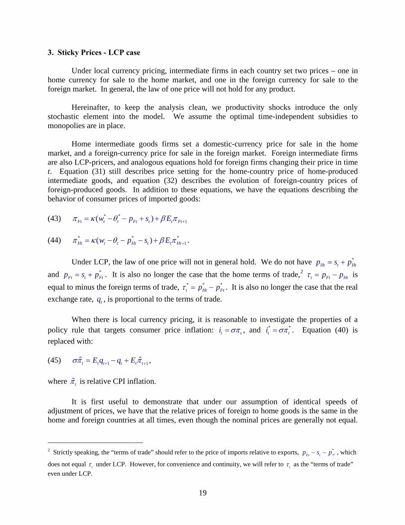
3. Sticky Prices - LCP case

Under local currency pricing, intermediate firms in each country set two prices – one in home currency for sale to the home market, and one in the foreign currency for sale to the foreign market. In general, the law of one price will not hold for any product.

Hereinafter, to keep the analysis clean, we productivity shocks introduce the only

stochastic element into the model. We assume the optimal time-independent subsidies to monopolies are in place. Home intermediate goods firms set a domestic-currency price for sale in the home market, and a foreign-currency price for sale in the foreign market. Foreign intermediate firms are also LCP-pricers, and analogous equations hold for foreign firms changing their price in time t. Equation (31) still describes price setting for the home-country price of home-produced intermediate goods, and equation (32) describes the evolution of foreign-country prices of foreign-produced goods. In addition to these equations, we have the equations describing the behavior of consumer prices of imported goods: (43) * *

1( )Ft t t Ft t t Ftw p s Eπ κ θ β π += − − + + (44) * *

1( ) *Ht t t Ht t t Hw p s Eπ κ θ β π t+= − − − + .

Under LCP, the law of one price will not in general hold. We do not have *

Ht t Htp s p= + and *

Ft t Ftp s p= + . It is also no longer the case that the home terms of trade,2 t Ft Htp pτ = − is equal to minus the foreign terms of trade, * *

t Ht*Ftp pτ = − . It is also no longer the case that the real

exchange rate, , is proportional to the terms of trade. tq When there is local currency pricing, it is reasonable to investigate the properties of a policy rule that targets consumer price inflation: ti tσπ= , and *

ti*tσπ= . Equation (40) is

replaced with: (45) 1 1ˆ ˆt t t t t tE q q Eσπ π+ += − + , where ˆtπ is relative CPI inflation.

It is first useful to demonstrate that under our assumption of identical speeds of adjustment of prices, we have that the relative prices of foreign to home goods is the same in the home and foreign countries at all times, even though the nominal prices are generally not equal.

2 Strictly speaking, the “terms of trade” should refer to the price of imports relative to exports, , which

does not equal

*HtFt tp s p− −

tτ under LCP. However, for convenience and continuity, we will refer to tτ as the “terms of trade” even under LCP.

19

That is, we can show *t tτ τ= − . Note that 1Ft Ht tπ π τ τ −− = − . Subtract equation (31) from (43) to

get: (46) * *

1 1( ( ) ) (t t t t t t t t t t tw w s E )τ τ κ θ θ τ β τ τ− +− = − − − + − + − . Then subtract equation (32) from (44), using * * * *

1Ht Ft t tπ π τ τ −− = − , to get: (47) * * * * * * *

1 ( ( ) ) (t t t t t t t t t t tw w s E )τ τ κ θ θ τ β τ τ−− = − − − − − + − . Add (46) and (47) together to get: , 1 1( )t t t t t tEκ β− +− = − + − where *

t t tτ τ≡ + . This equation has the solution * 0t t tτ τ= + = . From (31)-(32) and (43)-(44), we can derive: 1

ˆˆ ˆ(( 1)( ) ( 1) )t t t t tw s q E ˆt tπ κ γ γ θ β π += − − − − + + . Equation (33), which still holds under LCP, can be substituted in to get:

(48) 2

1( 1)ˆ 1 ( ) ( 1) (2 )( )t t t t tq q Eγ ζ ˆt tπ κ γ ζγ γ τ τ β π

ρ +

⎡ ⎤⎛ ⎞−= + − + − − − +⎢ ⎥⎜ ⎟

⎝ ⎠⎣ ⎦.

Equations (45) and (48) are dynamic equations for the real exchange rate, , and relative CPI inflation,

tqˆtπ . They are similar to equations (38) and (40) in the PCP model, which

determine the dynamics of the terms of trade and relative PPI inflation ( tτ and PPItπ ) in that

model. However, (45) and (48) do not fully characterize the dynamics of and tq ˆtπ , except in two special cases. The dynamic system must be completed by adding an equation to describe the dynamics of the terms of trade. To derive those dynamics, write equation (46) as:

(49) ( )1

1

( 1) ( ) 1 (2 ) (

( )

t t t t t t

t t t

q q

E

ζ γ )τ τ κ ζγ γ τ τρ

β τ τ

−

+

⎡ ⎤− −− = − − + − −⎢ ⎥

⎣ ⎦+ −

Equation (49) is a second-order difference equation, with a backward and a forward looking component. Equation (49) along with equations (45) and (48) constitute a fourth-order system that solves the dynamics of , tq ˆtπ , and tτ .

20

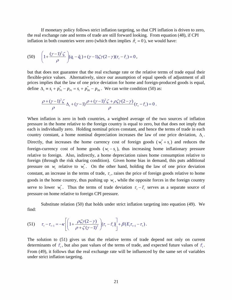
If monetary policy follows strict inflation targeting, so that CPI inflation is driven to zero, the real exchange rate and terms of trade are still forward looking. From equation (48), if CPI inflation in both countries were zero (which then implies ˆ 0tπ = ), we would have:

(50) 2( 1)1 ( ) ( 1) (2 )(t t t tq qγ ζ γ ζγ γ τ τ

ρ⎛ ⎞−+ − + − − −⎜ ⎟

⎝ ⎠) 0= ,

but that does not guarantee that the real exchange rate or the relative terms of trade equal their flexible-price values. Alternatively, since our assumption of equal speeds of adjustment of all prices implies that the law of one price deviation for home and foreign-produced goods is equal, define . We can write condition (50) as: * *

t t Ft Ft t Ht Hts p p s p pΔ ≡ + − = + −

2 2( 1) ( 1) (2 )( 1) ( ) 0t t

ρ γ ζ ρ γ ζ ρζγ γγ τρ ρ

+ − + − + −Δ + − − =tτ .

When inflation is zero in both countries, a weighted average of the two sources of inflation pressure in the home relative to the foreign country is equal to zero, but that does not imply that each is individually zero. Holding nominal prices constant, and hence the terms of trade in each country constant, a home nominal depreciation increases the law of one price deviation, tΔ . Directly, that increases the home currency cost of foreign goods ( ) and reduces the foreign-currency cost of home goods (

*tw s+ t

ttw s− ), thus increasing home inflationary pressure relative to foreign. Also, indirectly, a home depreciation raises home consumption relative to foreign (through the risk sharing condition). Given home bias in demand, this puts additional pressure on relative to . On the other hand, holding the law of one price deviation constant, an increase in the terms of trade,

tw *tw

tτ , raises the price of foreign goods relative to home goods in the home country, thus pushing up , while the opposite forces in the foreign country serve to lower . Thus the terms of trade deviation

tw*tw t tτ τ− serves as a separate source of

pressure on home relative to foreign CPI pressure.

Substitute relation (50) that holds under strict inflation targeting into equation (49). We find:

(51) 1 12

(2 )1 ( ) (( 1)t t t t t t tEρζγ γ )τ τ κ τ τ β τ

ρ ζ γ− +

⎡ ⎤⎛ ⎞−− = − + − + −⎢ ⎥⎜ ⎟+ −⎝ ⎠⎣ ⎦

τ .

The solution to (51) gives us that the relative terms of trade depend not only on current determinants of tτ , but also past values of the terms of trade, and expected future values of tτ . From (49), it follows that the real exchange rate will be influenced by the same set of variables under strict inflation targeting.

21

In this case of strict inflation targeting, tτ from (51) has a forward-looking and backward-looking component. The root for the forward looking component is given by

2(1 (1 ) 4 ) / 2a aβ β+ − − + − − β t, where a equals the coefficient on tτ τ− in equation (51). That forward-looking root is not affected by the monetary policy, and will be large, approaching β as goes to zero. That is, even with complete inflation targeting, news about future values of

κ

tτ will have a strong influence on tτ . Indeed, this result is more general. The dynamic system for the terms of trade, inflation,

and the real exchange rate is given by equations (45), (48), and (49). In this system, there are three forward-looking roots and one backward-looking. The Appendix shows that for any degree of inflation targeting (that is, for any value of σ ), the largest forward-looking root is greater than or equal to β as goes to zero. Conversely, when inflation targeting is weak (that is, as

κ1σ → ), the largest forward looking root approaches unity. The largest forward looking root

determines ultimately the weight that news about the future receives in the determination of the terms of trade. Under LCP, this root will tend to be large; therefore, news about future productivity levels will have a large influence on current relative prices.

News affects the terms of trade and the real exchange rate. For example, suppose agents receive news at time t about some future changes in productivity that influence t jτ + . Under strict CPI inflation targeting, we see from equation (51) that the current terms of trade, tτ , is still affected by this news. Price setters adjust prices today in anticipation of that future change in productivity. Suppose, for example, that t jτ + rises – perhaps a positive home productivity change will drive down the equilibrium relative price of home goods in the future. That leads am increase in tτ , but this is not efficient because tτ has not changed, so t tτ τ> . The drop in the relative price of home goods tends to contribute to an increase in home relative to foreign CPI inflation because of home bias in preferences. From equation (50), under strict inflation targeting, this increase in tτ must be offset by a real appreciation – an drop in –to keep CPI inflation unchanged. So the real exchange rate is also responding to news, even under strict inflation targeting, and deviates from .

tq

tq tq In fact the flexible price equilibrium is not attainable under policies that target only inflation, whether it be CPI inflation or some other type of inflation. For example, a policy such as the one described in the PCP model that forces Htπ and *

Ftπ to zero will still leave us with forward looking real exchange rate and terms of trade. The problem with inflation targeting alone is easy to understand. Suppose monetary policymakers set Htπ , Ftπ , *

Ftπ , and *Htπ all

equal to zero. Then Htp , Ftp , *Ftp , and *

Htp would all be constant, but it is not optimal to have all of these prices constant. Efficient allocation requires that the terms of trade, t Ft Htp pτ = − and * *

t Ht*Ftp pτ = − respond to productivity changes.

Suppose that policymakers follow a policy of strict CPI inflation targeting, so that CPI inflation rates in each country ( tπ and *

tπ ) are driven to zero. Under these conditions, if

22

policymakers could also drive the real exchange rate toward its flexible-price value, qt qt=0

, then from equation (50) shows that the terms of trade distortion is eliminated: t tτ τ−

0t

= . In this case, the forward-looking reaction of the terms of trade and the real exchange rate would be eliminated. The policymaker under LCP cannot achieve the targets of π = , * 0tπ = , and

simultaneously. Since all four prices, tq q= t Htp , Ftp , *Ftp , and *

Htp , have a backward looking component, it is not possible to have relative prices respond optimally to productivity shocks.

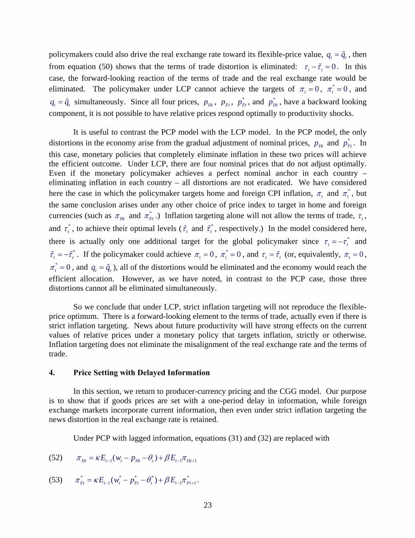
It is useful to contrast the PCP model with the LCP model. In the PCP model, the only

distortions in the economy arise from the gradual adjustment of nominal prices, *FtpHtp and . In

this case, monetary policies that completely eliminate inflation in these two prices will achieve the efficient outcome. Under LCP, there are four nominal prices that do not adjust optimally. Even if the monetary policymaker achieves a perfect nominal anchor in each country – eliminating inflation in each country – all distortions are not eradicated. We have considered here the case in which the policymaker targets home and foreign CPI inflation, *

tπ and tπ , but the same conclusion arises under any other choice of price index to target in home and foreign currencies (such as Htπ and *

Ftπ .) Inflation targeting alone will not allow the terms of trade, tτ , and *

tτ , to achieve their optimal levels ( tτ and *tτ , respectively.) In the model considered here,

there is actually only one additional target for the global policymaker since *t tτ τ= − and

* *tπ 0t tτ τ= − . If the policymaker could achieve 0tπ = , = , and t t (or, equivalently, 0τ=τ tπ = ,

, and ), all of the distortions would be eliminated and the economy would reach the efficient allocation. However, as we have noted, in contrast to the PCP case, those three distortions cannot all be eliminated simultaneously.

* 0tπ = tq = tq

So we conclude that under LCP, strict inflation targeting will not reproduce the flexible-

price optimum. There is a forward-looking element to the terms of trade, actually even if there is strict inflation targeting. News about future productivity will have strong effects on the current values of relative prices under a monetary policy that targets inflation, strictly or otherwise. Inflation targeting does not eliminate the misalignment of the real exchange rate and the terms of trade. 4. Price Setting with Delayed Information In this section, we return to producer-currency pricing and the CGG model. Our purpose is to show that if goods prices are set with a one-period delay in information, while foreign exchange markets incorporate current information, then even under strict inflation targeting the news distortion in the real exchange rate is retained. Under PCP with lagged information, equations (31) and (32) are replaced with

(52) 1 1( ) 1Ht t t Ht t t HE w p E tπ κ θ β− −= − − + π

*

+ (53) * * * *

1 1( )Ft t t Ft t t FtE w p E 1π κ θ β− −= − − + π + .

23

PPI inflation in each country, Htπ and *

Ftπ , are predetermined: their time t levels depend only on t-1 information. We can write relative PPI inflation as: (54) 1 1ˆ ˆ( ) 1

PPI PPIt t t t tE E tπ κ τ τ β π− −= − + + ,

replacing equation (34). We assume that current information is used by households in forming inflation expectations. The Euler equations, (35) and (36) are unchanged. We can combine them as above with the policy rule to write: (55) 1 1ˆ ˆPPI PPI

t t t t t tE Eσπ τ τ π+ += − + , which is identical to equation (40) except that we have dropped the liquidity disturbances. If we take time t-1 expectations of equation (55), we get: (56) 1 1 1 1ˆ ˆ( )PPI PPI

t t t t t tE Eσπ τ τ− + − += − + π . Equations (54) and (56) form a two-equation dynamic system in the t-1 expected values of tτ and

ˆ PPItπ (the

1 t

latter of which equals its actual value.) That system’s dynamics are described as in equation (41) above. We can write: (57) 1 1 1t t t t tE E E τ− − += +z B z C − ,

where all variables are defined as above except for C, which we now define by 1

1

κσκ

σκσκ

−⎡ ⎤⎢ ⎥+≡ ⎢ ⎥⎢ ⎥⎢ ⎥+⎣ ⎦

C ,

because we have dropped the liquidity disturbances. Analogous to equation (42), we can write a forward-looking solution to (57): (58) , 2 3

1 1 1 1 1 2 1 3t t t t t t t t t tE E E E Eτ τ τ τ− − − + − + − += + + + +z C BC B C B C … where B is defined as above. B has the same diagonal decomposition as previously, so the roots of system (58) – the “discount factors” – are the same as before. Since inflation is predetermined, so 1 ˆ ˆPPI PPI

t t tE π π− = , equation (58) determines relative inflation. But it only determines the expected terms of trade, 1tE tτ− . To get the actual terms of trade, subtract (56) from (55) to get: (59) 1 1 1 1 1 1ˆ ˆ 1

PPI PPIt t t t t t t t t tE E E Eτ τ τ τ π π− + − + + −= + − + − +

24

Leading equation (58) one period, and then subtracting t-1 expectations, we get: (60) , 2 3

1 1 2 3 4D D D D Dt t t t t t t t t tE E E E Eτ τ τ τ+ + + + += + + + +z C BC B C B C …

where . The second equation in the system (60) gives us the term 1

Dt t j t t j t t jE x E x E x+ + −≡ −

1 1 1t tE+

t tEτ τ+ − +− from equation (59), the news at time t about the terms of trade at time t+1. Strict inflation targeting, σ →∞ , drives the discount factors in equation (58) to zero, just as before. But this time, it does not imply there is no news effect on the terms of trade. Equation (58) determines 1tE tτ− . From equation (58), strict inflation targeting implies: (61) 1 1t t tE E tτ τ− −= . But from equation (59), the actual terms of trade incorporates news about 1tτ + . Suppose the news that arrives at time t+1 is about 1tτ + . From equation (60), the news effect on tτ is:

(62) 1 1 11 1t t t tDt tE E Eστ κ ττ

σκ+ − + +− =+

.

Equation (62) shows that strict inflation targeting maximizes the distortion to tτ from the news about 1tτ + . However, note that news about 1tτ + may also contain news about jtτ + , 1j > . Strict

inflation targeting drives , so it eliminates the influence 0→BC Dt t jE τ + , , on 1>j tτ . Using

equations (59), (61), and (62), we can write the distortion in the terms of trade under strict inflation targeting (σ →∞ ) as: (63) 1

D Dtt t t ttE Eτ τ τ τ +− = − + .

The first term on the right-hand-side of equation (63) will be large when there is not much news. That is, it will be small when agents know little about tτ until time t. If tτ were known completely one period in advance, then D

t tE τ would be zero. But in an environment where agents learn about productivity shocks a period in advance, 1t t

DE τ + is large. The bottom line is that strict inflation targeting does not eliminate all distortions, and does not eliminate the effect of news on the terms of trade and the real exchange rate. It may actually worsen the distortion. There are potential gains from targeting the real exchange rate. The next section investigates a model that combines both LCP and lagged information in price setting.

25

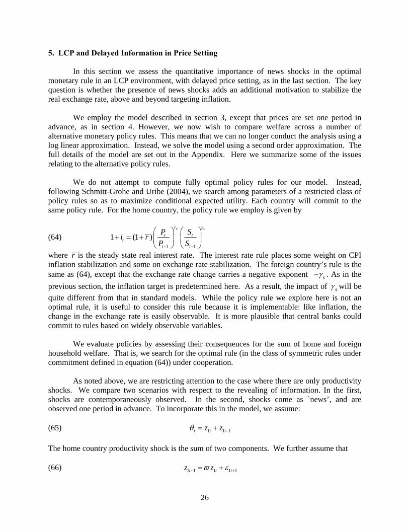
5. LCP and Delayed Information in Price Setting In this section we assess the quantitative importance of news shocks in the optimal monetary rule in an LCP environment, with delayed price setting, as in the last section. The key question is whether the presence of news shocks adds an additional motivation to stabilize the real exchange rate, above and beyond targeting inflation. We employ the model described in section 3, except that prices are set one period in advance, as in section 4. However, we now wish to compare welfare across a number of alternative monetary policy rules. This means that we can no longer conduct the analysis using a log linear approximation. Instead, we solve the model using a second order approximation. The full details of the model are set out in the Appendix. Here we summarize some of the issues relating to the alternative policy rules. We do not attempt to compute fully optimal policy rules for our model. Instead, following Schmitt-Grohe and Uribe (2004), we search among parameters of a restricted class of policy rules so as to maximize conditional expected utility. Each country will commit to the same policy rule. For the home country, the policy rule we employ is given by

(64)1 1

1 (1 )s

t tt

t t

P Si rP S

πγ γ

− −

⎛ ⎞ ⎛ ⎞+ = + ⎜ ⎟ ⎜ ⎟

⎝ ⎠ ⎝ ⎠

where r is the steady state real interest rate. The interest rate rule places some weight on CPI inflation stabilization and some on exchange rate stabilization. The foreign country’s rule is the same as (64), except that the exchange rate change carries a negative exponent sγ− . As in the previous section, the inflation target is predetermined here. As a result, the impact of πγ will be quite different from that in standard models. While the policy rule we explore here is not an optimal rule, it is useful to consider this rule because it is implementable: like inflation, the change in the exchange rate is easily observable. It is more plausible that central banks could commit to rules based on widely observable variables. We evaluate policies by assessing their consequences for the sum of home and foreign household welfare. That is, we search for the optimal rule (in the class of symmetric rules under commitment defined in equation (64)) under cooperation. As noted above, we are restricting attention to the case where there are only productivity shocks. We compare two scenarios with respect to the revealing of information. In the first, shocks are contemporaneously observed. In the second, shocks come as `news’, and are observed one period in advance. To incorporate this in the model, we assume: (65) 1 1t t tz z 1θ −= + The home country productivity shock is the sum of two components. We further assume that (66) 1 1 1 1 1t tz z tϖ ε+ += +

26

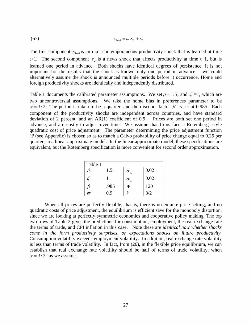
(67) 2 1 2 2t tz z tϖ ε+ = + The first component 1 1tε + is an i.i.d. contemporaneous productivity shock that is learned at time t+1. The second component 2tε is a news shock that affects productivity at time t+1, but is learned one period in advance. Both shocks have identical degrees of persistence. It is not important for the results that the shock is known only one period in advance – we could alternatively assume the shock is announced multiple periods before it occurrence. Home and foreign productivity shocks are identically and independently distributed. Table 1 documents the calibrated parameter assumptions. We set 1.5ρ = , and ζ =1, which are two uncontroversial assumptions. We take the home bias in preferences parameter to be

3 / 2γ = . The period is taken to be a quarter, and the discount factor β is set at 0.985. Each component of the productivity shocks are independent across countries, and have standard deviation of 2 percent, and an AR(1) coefficient of 0.9. Prices are both set one period in advance, and are costly to adjust over time. We assume that firms face a Rotemberg- style quadratic cost of price adjustment. The parameter determining the price adjustment function

(see Appendix) is chosen so as to match a Calvo probability of price change equal to 0.25 per quarter, in a linear approximate model. In the linear approximate model, these specifications are equivalent, but the Rotemberg specification is more convenient for second order approximation.

Ψ

Table 1 ρ 1.5

1εσ 0.02

ζ 1 2ε

σ 0.02 β .985 Ψ 120 ϖ 0.9 γ 3/2

When all prices are perfectly flexible; that is, there is no ex-ante price setting, and no quadratic costs of price adjustment, the equilibrium is efficient save for the monopoly distortion, since we are looking at perfectly symmetric economies and cooperative policy making. The top two rows of Table 2 gives the predictions for consumption, employment, the real exchange rate the terms of trade, and CPI inflation in this case. Note these are identical now whether shocks come in the form productivity surprises, or expectations shocks on future productivity. Consumption volatility exceeds employment volatility. In addition, real exchange rate volatility is less than terms of trade volatility. In fact, from (26), in the flexible price equilibrium, we can establish that real exchange rate volatility should be half of terms of trade volatility, when

3 / 2γ = , as we assume.

27

Table 2 cσ hσ rerσ τσ πσ

πγ sγ

Fully flexible prices

1

2 .02εσ = 2

2 0εσ = 0.027 0.006 0.034 0.067 - - -

Fully flexible prices

1

2 0εσ = 2

2 .02εσ = 0.027 0.006 0.034 0.067 - - -

Sticky Prices 1

2 .02εσ = 2

2 0εσ = 0.032 0.015 0.0630 0.034 0 ∞ 0

Sticky Prices 1

2 0εσ = 2

2 .02εσ = 0.0250 0.02 0.0375 0.0411 .005 1.6 0.8

The last two rows of Table 2 illustrate the results for optimal monetary policy in the case of contemporaneous productivity shocks and news shocks, respectively. The optimal policy rules are obtained by searching across the parameters

πγ and sγ which maximize conditional expected

utility. When all shocks are contemporaneous productivity shocks, we find that an optimal monetary policy rule is to stabilize each country’s CPI. The monetary policy rule does this by setting

πγ arbitrarily high. Note that this does not support the fully flexible price equilibrium however. In fact, consumption and output volatility is higher than in the flexible price equilibrium. In addition, real exchange rate volatility is now almost double that in the flexible price equilibrium, while terms of trade volatility is half that of the flexible price equilibrium. In the case of contemporaneous productivity shocks, there is no additional benefit from targeting the exchange rate – the optimal value of sγ is zero. The results are quite different in the case of productivity news shocks. In this case, we find it is not optimal to stabilize the CPI. Stabilizing the CPI exacerbates the inefficient time t response to news shocks about time t+1 productivity. At the same time, such a policy leads to excessive real exchange rate volatility. The optimal policy is a combination which targets both the CPI and the exchange rate. In fact, the optimal weight on CPI inflation is only 1.6. In order to dampen the influence of news shock on contemporaneous variables, there is an additional benefit from targeting the exchange rate in this case. The optimal value of sγ is 0.8. The end result is that equilibrium real exchange rate volatility is below terms of trade volatility, and almost equal to the value in the flexible price equilibrium. CPI inflation volatility is positive. Consumption volatility is lower than in the case of contemporaneous productivity shocks. We can compare the welfare gains from targeting the real exchange rate to the gains from inflation targeting alone, when agents receive news about future productivity. If we restrict sγ to equal zero, the optimal weight on CPI inflation is still 1.6. The additional welfare gains from letting sγ be unrestricted are 21% of the gains from moving from weak inflation targeting (a

28

weight on CPI inflation of 1.1) to the optimal value of 1.6. So, while inflation targeting alone delivers most of the welfare benefits of the optimal policy rule, the additional benefits of moderating fluctuations in the exchange rate are far from negligible. 6. Conclusions The examples in the models of the paper imply that the exchange rate should be insulated against the impact of shocks to expectations of future productivity. This is because with sticky nominal goods prices, exchange rate movements affect relative prices, and in the models we analyze, efficient relative prices are independent of future productivity. . The model as formulated makes an assumption of complete markets. When market are incomplete, news shocks may generate wealth effects that alter current relative prices, even when all nominal prices are fully flexible. This makes the optimal policy response to news shocks less clear. But it is still not self-evident that under a policy that ignores news shocks, the exchange rate will move in a manner consistent with efficient adjustment. More generally, an optimal cooperative monetary policy may wish to eliminate these wealth effects in any case, and this would be likely to involve dampening the exchange rate impacts of news shocks. It is frequently argued that flexible exchange rates can lead to efficient changes in relative prices when nominal prices adjust sluggishly, but when capital is mobile, exchange rate movements do not effectively substitute for price changes. Experience with floating exchange rates has shown us that expectations can lead to large and prolonged swings in exchange rates that do not correspond to any current changes in tastes or technology. Indeed, asset markets may be correctly pricing the effects of future changes in fundamentals, but the resulting allocations still are not efficient. Exchange rates cannot simultaneously achieve the asset market equilibrium that reflects news about the future relative values of currencies and the goods market equilibrium that reflects efficient relative prices.

29

References

Barro, Robert and Robert G. King. 1984. “Time-Separable Preference and Intertemporal-Substitution Models of Business Cycles,” Quarterly Journal of Economics, 99:4, 817-839.

Benigno, Gianluca. 2004. “Real Exchange Rate Persistence and Monetary Policy Rules,”

Journal of Monetary Economics 51, 573-502. Bernanke, Ben S., and Mark Gertler. 1999. “Monetary Policy and Asset Volatility,” Federal

Reserve Bank of Kansas City Economic Review 84, 17-52. Bernanke, Ben S., and Mark Gertler. 2001. “Should Central Banks Respond to Movements in

Asset Prices?” American Economic Review Papers and Proceedings, 253-257. Betts, Caroline, and Michael B. Devereux. 1996. “The Exchange Rate in a Model of Pricing-to-

Market,” European Economic Review 40, 1007-1021. Blanchard, Olivier, and Jordi Gali. 2007. “Real Wage Rigidities and the New Keynesian

Model,” Journal of Money, Credit and Banking 39, 35-65. Clarida, Richard; Jordi Gali; and Mark Gertler. 2002. “A Simple Framework for International

Monetary Policy Analysis,” Journal of Monetary Economics 49:5, 879-904. Devereux, Michael B. and Charles Engel. 2003. “Monetary Policy in the Open Economy

Revisited: Price Setting and Exchange Rate Flexibility,” Review of Economic Studies, 70:4, 765-783.

Erceg, Christoper; Dale Henderson; and, Andrew Levin. 2000. “Optimal Monetary Policy with

Staggered Wage and Price Contracts,” Journal of Monetary Economics 46, 281-313. Klenow, Peter J., and Jonathan L. Willis. 2007. “Sticky Information and Sticky Prices,” Journal

of Monetary Economics 54, supplement 1, 79-99. Mankiw, N. Gregory, and Ricardo Reis. 2002. “Sticky Information Versus Sticky Prices: A

Proposal to Replace the New Keynesian Phillips Curve,” Quarterly Journal of Economics 117, 1295-1328.

Schmitt-Grohe, Stephanie and Martin Uribe, 2004 “Optimal Operational Monetary Policy in the

Christiano-Eichenbaum-Evans Model of the US Business Cycle”, Duke University, mimeo.

West, Kenneth. 1988. “Dividend Innovations and Stock Price Volatility,” Econometrica, 56:1,

37-61. Woodford, Michael. 2003. Interest and Prices: Foundations of a Theory of Monetary Policy,

(Princeton: Princeton University Press).

30

31

Zbaracki, Mark J.; Mark Ritson; Daniel Levy; Santanu Dutta; and, Mark Bergen. 2004.

“Managerial and Customer Costs of Price Adjustment: Evidence from Industrial Markets,” Review of Economics and Statistics 86, 514-533.