Embed Size (px)
Citation preview

Misspecified Recovery∗
Jaroslav Borovicka
New York University
Lars Peter Hansen
University of Chicago and NBER
Jose A. Scheinkman
Columbia University, Princeton University and NBER
October 1, 2015
Abstract
Asset prices contain information about the probability distribution of future states and the
stochastic discounting of those states as used by investors. To better understand the challenge in
distinguishing investors’ beliefs from risk-adjusted discounting, we use Perron–Frobenius The-
ory to isolate a positive martingale component of the stochastic discount factor process. This
component recovers a probability measure that absorbs long-term risk adjustments. When the
martingale is not degenerate, surmising that this recovered probability captures investors’ be-
liefs distorts inference about risk-return tradeoffs. Stochastic discount factors in many structural
models of asset prices have empirically relevant martingale components.
∗We thank Fernando Alvarez, David Backus, Ravi Bansal, Anmol Bhandari, Peter Carr, Xiaohong Chen, Ing-HawCheng, Mikhail Chernov, Kyle Jurado, Francois Le Grand, Stavros Panageas, Karthik Sastry, Kenneth Singleton,Johan Walden, Wei Xiong and the anonymous referees for useful comments.

Asset prices are forward looking and encode information about investors’ beliefs. This leads re-
searchers and policy makers to look at financial market data to gauge the views of the private sector
about the future of the macroeconomy. It has been known, at least since the path-breaking work of
Arrow, that asset prices reflect a combination of investors’ risk aversion and the probability distri-
butions used to assess risk. In dynamic models, investors’ risk aversion is expressed by stochastic
discount factors that include compensations for risk exposures. In this paper, we ask what can be
learned from the Arrow prices about investors’ beliefs. Data on asset prices alone are not sufficient
to identify both the stochastic discount factor and transition probabilities without imposing addi-
tional restrictions. This additional information could be time series evidence on the evolution of
the Markov state, or it could be information on the market-determined stochastic discount factors.
In a Markovian environment, Perron–Frobenius Theory selects a single transition probability
compatible with asset prices. This Perron–Frobenius apparatus has been used in previous research
in at least two manners. First, Hansen and Scheinkman (2009) showed that this tool identifies
a probability measure that reflects the long-term implications for risk pricing under rational ex-
pectations. We refer to this probability as the long-term risk neutral probability since the use
of this measure renders the long-term risk-return tradeoffs degenerate. Hansen and Scheinkman
(2009) purposefully distinguish this constructed transition probability from the underlying time
series evolution. The ratio of the recovered to the true probability measure is manifested as a
non-trivial martingale component in the stochastic discount factor process. Second, Ross (2015)
applied Perron–Frobenius Theory to identify or to “recover” investors’ beliefs. Interestingly, this
recovery does not impose rational expectations, thus the resulting Markov evolution could reflect
subjective beliefs of investors and not necessarily the actual time series evolution.
In this paper we delineate the connection between these seemingly disparate results. We make
clear the special assumptions that are needed to guarantee that the transition probabilities recovered
using Perron–Frobenius Theory are equal to the subjective transition probabilities of investors or
to the actual probabilities under an assumption of rational expectations. We show that in some
often used economic settings — with permanent shocks to the macroeconomic environment or
with investors endowed with recursive preferences — the recovered probabilities differ from the
subjective or actual transition probabilities, and provide a calibrated workhorse asset pricing model
that illustrates the magnitude of these differences.
Section 1 illustrates the challenge of identifying the correct probability measure from asset
market data in a finite-state space environment. While the finite-state Markov environment is too
constraining for many applications, the discussion in this section provides an overview of some of
the main results in this paper. In particular, we show that:
• the Perron–Frobenius approach recovers a probability measure that absorbs long-term risk
prices;
• the density of the Perron–Frobenius probability relative to the physical probability gives rise
to a martingale component to the stochastic discount factor process;
1

• under rational expectations, the stochastic discount factor process used by Ross (2015) implies
that this martingale component is a constant.
To place these results in a substantive context, we provide prototypical examples of asset pricing
models that show that a nontrivial martingale component arises from (i) permanent shocks to
the consumption process or (ii) continuation value adjustment that appear when investors have
recursive utilities.
In subsequent sections we establish these insights in greater generality, a generality rich enough
to include many existing structural Markovian models of asset pricing. The framework for this
analysis, which allows for continuous state spaces and a richer information structure, is introduced
in Section 2. In Section 3, we extend the Perron–Frobenius approach to this more general setting.
Provided we impose an additional ergodicity condition, this approach identifies a unique probability
measure captured by a martingale component to the stochastic discount factor process.
In Section 4, we show the consequences of using the probability measure recovered by the use
of the Perron–Frobenius Theory when making inferences on the risk-return tradeoff. The recovered
probability measure absorbs the martingale component of the original stochastic discount factor
and thus the recovered stochastic discount factor is trend stationary. Since the factors determining
long-term risk adjustments are now absorbed in the recovered probability measure, assets are priced
as if long-term risk prices were trivial. This outcome is the reason why we refer to the probability
specification revealed by the Perron–Frobenius approach as the long-term risk neutral measure.
Section 5 illustrates the impact of a martingale component to the stochastic discount factor in a
workhorse asset pricing model that features long-run risk.
Starting in Section 6, we characterize the challenges in identifying subjective beliefs from asset
prices. Initially we pose the fundamental identification problem: data on asset prices can only
identify the stochastic discount factor up to an arbitrary strictly positive martingale, and thus
the probability measure associated with a stochastic discount factor remains unidentified without
imposing additional restrictions or using additional data. We also extend the analysis of Ross
(2015) to this more general setting. By connecting to the results in Section 3, we demonstrate
in Section 6 that the martingale component to the stochastic discount factor process must be
identically equal to one for Ross (2015)’s procedure to reveal the subjective beliefs of investors.
Under these beliefs, the long-term risk-return tradeoff is degenerate. Some might wonder whether
the presence of a martingale component could be circumvented in practice by approximating the
martingale by a highly persistent stationary process. In Section 7 we show that when we extend
the state vector to address this approximation issue identification of beliefs becomes tenuous. In
Section 8, we provide a unifying discussion of the empirical approaches that quantify the impact
of the martingale components to stochastic discount factors when an econometrician does not use
the full array of Arrow prices. We also suggest other approaches that connect subjective beliefs to
the actual time series evolution of the Markov states. Section 9 concludes.
2
1 Illustrating the identification challenge
There are multiple approaches for extracting probabilities from asset prices. For instance, risk
neutral probabilities (e.g., see Ross (1978) and Harrison and Kreps (1979)) and closely related
forward measures are frequently used in financial engineering. More recently, Perron–Frobenius
Theory has been applied by Backus et al. (1989), Hansen and Scheinkman (2009) and Ross (2015) to
study asset pricing — the last two references featuring the construction of an associated probability
measure. Hansen and Scheinkman (2009) and Ross (2015) have rather different interpretations of
this measure, however. Ross (2015) identifies this measure with investors’ beliefs while Hansen and
Scheinkman (2009) use it to characterize long-term contributions to risk pricing. Under this second
interpretation, Perron–Frobenius Theory features an eigenvalue that dominates valuation over long
investment horizons, and the resulting probability measure targets the valuation of assets that pay
off in the far future as a point of reference. Following Hansen and Scheinkman (2014), in this section
we illustrate the construction of the alternative probability measure using matrices associated with
finite-state Markov chains and we explore some simple example economies to understand better
the construction of a probability measure based on Perron–Frobenius Theory.
Let X be a discrete time, n-state Markov chain with transition matrix P = [pij]. We suppose
that these are the actual transition probabilities that govern the evolution of the Markov process.
We identify state i with a coordinate vector ui with a single one in the i-th entry. The analyst infers
the prices of one-period Arrow claims from data. We represent this input as a matrix Q = [qij]
that maps a payoff tomorrow specified as a function of tomorrow’s state j into a price in state i
today. Since there are only a finite number of states, the payoff and price can both be represented
as vectors. In particular, the vector of Arrow prices given the current realization x of the Markov
state is x′Q. The entries of this vector give the prices of claims payable in each of the possible
states tomorrow. Any state that cannot be realized tomorrow given the current state x is assigned
a price of zero today.
Asset pricing implications are represented conveniently using stochastic discount factors. Stochas-
tic discount factor encode adjustments for uncertainty by discounting the next-period state differ-
entially. Risk premia are larger for states that are more heavily discounted. In this finite-state
Markov environment, we compute
sij =qijpij
(1)
provided that pij > 0. The definition of sij is inconsequential if pij = 0. Given a matrix S = [sij],
the stochastic discount factor process has the increment:
St+1
St= (Xt)
′SXt+1. (2)
The stochastic discount factor process S = St : t = 0, 1, 2, ... is initialized at S0 = 1 and
3

accumulates the increments given by (2):
St =
t∏
τ=1
(Xτ−1)′ SXτ .
Observe that St depends on the history of the state from 0 to t. With this notation, we have two
ways to write the period-zero price of a claim to a vector of state-dependent payoffs f ·Xt at time t.
Qtf · x = E [St (f ·Xt) | X0 = x] .
Given the matrix P, possibly determined under rational expectations by historical data and
stochastic discount factors implied by an economic model, Arrow prices are given by inverting
equation (1):
qij = sijpij. (3)
A question that we explore is what we can learn about beliefs from Arrow prices. Market sentiments
or beliefs are part of the discourse for both public and private sectors. We study this question by
replacing the assumption of rational expectations with an assumption of subjective beliefs.
Unfortunately, there is considerable flexibility in constructing probabilities from the Arrow
prices alone. Notice that Q has n × n entries. P has n × (n − 1) free entries because row sums
have to add up to one. In general the stochastic discount factor introduces n× n free parameters
sij, i, j = 1, . . . , n. Since the Arrow prices are the products given in formula (3), there are multiple
solutions for probabilities and stochastic discount factors that are consistent with Arrow prices.1
To depict this flexibility, represent alternative transition probabilities by
pij = hijpij
where hij > 0 and∑n
j=1 hijpij = 1 for i = 1, 2, ..., n. Form a matrix H = [hij ] and a positive
process Ht : t = 0, 1, ... with increments
Ht+1
Ht= (Xt)
′HXt+1.
The restrictions on the entries of H restrict the increments to satisfy
E
[Ht+1
Ht| Xt = x
]= 1.
Accumulating the increments:
Ht = H0
t∏
τ=1
(Xτ−1)′ HXτ .
1The simple counting requires some qualification when Q has zeros. For instance, when qij = 0, then pij = 0 inorder to prevent arbitrage opportunities.
4
The initial distribution of X0 together with the transition matrix P define a probability P over
realizations of the process X. Because hij is obtained as a ratio of probabilities, H is a positive
martingale under P for any positive specification of H0 as a function of X0.
Using the positive martingale H to induce a change of measure, we obtain the probability P :
P (Xt = xt) = P (Xt = xt)H0
t∏
τ=1
(xτ−1)′Hxτ .
for alternative possible realizations xt = (x0, x1, ..., xt) of Xt = (X0,X1, . . . Xt). In this formula, we
presume that EH0 = 1, and we use H0 in order for P to include a change in the initial distribution
of X0. Thus the random variable H0 modifies the distribution of X0 under P vis-a-vis P , and P
specifies the altered transition probabilities. Most of our analysis conditions on X0, in which case
the choice of H0 is inconsequential and H0 can be set to one for simplicity.
For each choice of the restricted matrix H, we may form the corresponding state-dependent
discount factors sij = sij/hij by applying formula (1). By construction
qij = sijpij = sij pij . (4)
Given flexibility in constructing H = [hij ], we have multiple ways to recover probabilities from
Arrow prices.
We may confront this multiplicity by imposing restrictions on the stochastic discount factors.
As we shall argue, the resulting constructions provide valuable tools for asset pricing even when
these probabilities are not necessarily the same as those used by investors. In what follows we
consider two alternative restrictions:
(i) Risk-neutral pricing:
si,j = qi (5)
for positive numbers qi, i = 1, 2, ..., n. This restriction exploits the pricing of one-period
discount bonds.
(ii) Long-term risk pricing:
sij = exp(η)mj
mi(6)
for positive numbers mi, i = 1, 2, ..., n and a real number η that is typically negative. The
mi’s need only be specified up to a scale factor and the resulting vector can be normalized
conveniently. As we show below, this restriction helps us characterize long-term pricing
implications.
In both cases we reduce the number of free parameters in the matrix S from n2 to n, making
identification of the probabilities possible. As we show, each approach has an explicit economic
interpretation but the matrices of transition probabilities that are recovered do not necessarily
coincide with those used by investors or with the actual Markov state dynamics. In the first case
5

the difference between the inferred and true probabilities reflects a martingale that determines
the one-period risk adjustments in financial returns. As we show below, in the second case the
difference between the inferred and true probabilities reflects a martingale that determines long-
term risk adjustments in pricing stochastically growing cash flows.
1.1 Risk-neutral probabilities
Risk-neutral probabilities are used extensively in the financial engineering literature. These proba-
bilities are a theoretical construct used to absorb the local or one-period risk adjustments and are
determined by positing a fictitious “risk-neutral” investor. The stochastic discount factor given by
(5) reflects the fact that all states j tomorrow are discounted equally. In order to satisfy pricing
restrictions (3), the risk-neutral transition probabilities must be given by
pij =qijqi.
Since rows of a probability matrix have to sum up to one, it necessarily follows that qi =∑n
j qij,
which is the price of a one-period discount bond in state i.
The risk-neutral probabilities [pij ] can always be constructed and used in conjunction with
discount factors [sij ]. By design the discount factors are independent of state j, reflecting the
absence of risk adjustments conditioned on the current state. In contrast, one-period discount bond
prices can still be state-dependent and this dependence is absorbed into the subjective discount
factor of the fictitious-risk neutral investor. While it is widely recognized that the risk-neutral
distribution is distinct from the actual probability distribution, some have argued that the risk-
neutral dynamics remain interesting for macroeconomic forecasting precisely because they do embed
risk adjustments.2
When short-term interest rates are state-dependent, forward measures are sometimes used in
valuation. Prices of t-period Arrow securities, q[t]ij , are the entries of the t-th power of the matrix
Q. The t-period forward probability measure given the current state i is
Pt =
[q[t]ij∑n
j=1 q[t]ij
].
The denominator used for scaling the Arrow prices is now the price of a t-period discount bond.
While the forward measure is of direct interest,
Pt 6=(P)t, (7)
2Narayana Kocherlakota, President of the Federal Reserve Bank of Minneapolis, during a speech to the MitsuiFinancial Symposium in 2012 asks and answers: “How can policymakers formulate the needed outlook for marginalnet benefits? . . . I argue that policymakers can achieve better outcomes by basing their outlooks on risk-neutral
probabilities derived from the prices of financial derivatives.” See Hilscher et al. (2014) for a study of public debtusing risk-neutral probabilities.
6

when one-period bond prices are state dependent. Variation in one-period interest rates contributes
to risk adjustment over longer investment horizons, and as a consequence the construction of risk-
neutral probabilities is horizon-dependent.
1.2 Long-term pricing
We study long-term pricing of cash flows associated with fixed income securities using Perron–
Frobenius Theory. When there exists a λ > 0 such that the matrix∑
∞
t=0 λtQt has all entries that
are strictly positive, the largest (in absolute value) eigenvalue of Q is unique and positive and thus
can be written as exp(η), and has a unique associated right eigenvector e, which has strictly positive
entries. Every non-negative eigenvector of Q is a scalar multiple of e. We denote the ith entry of e
as ei. Typically, η < 0 to reflect time discounting of future payoffs over long investment horizons.
Recall that we may evaluate t-period claims by applying the matrix Q t-times in succession.
From the Perron–Frobenius theory for positive matrices:
limt→∞
exp(−ηt)Qtf = (f · e∗)e
where e∗ is the corresponding positive left eigenvector of Q. Applying this formula, the large t
approximation to the rate of discount on an arbitrary security with positive payoff f · Xt in t
periods is −η. Similarly, the one-period holding-period return on this limiting security is:
limt→∞
Qt−1f ·X1
Qtf ·X0= exp(−η) e ·X1
e ·X0.
The eigenvector e and the associated eigenvalue also provide a way to construct a probability
transition matrix given Q. Set
pij := exp(−η)qijejei. (8)
Notice that since Qe = exp(η)e,
n∑
j=1
pij = exp(−η) 1ei
n∑
j=1
qij ej = 1.
Thus P = [pij ] is a transition matrix. Moreover,
qij = exp(η)eiejpij = sij pij.
Thus we have used the eigenvector e and the eigenvalue η to construct a stochastic discount factor
that satisfies (6) together with a probability measure that satisfies (3). The probability measure
constructed in this fashion absorbs the compensations for exposure to long-term components of
risk. Conversely, if one starts with an S and P that satisfy (3) and (6) then it is straightforward
7

to show that the vector with entries ei = 1/mi is an eigenvector of Q.3
If we start with the t-period Arrow prices in the matrix Qt instead of the one-period Arrow
prices in the matrix Q, then
Qte = exp(ηt)e
for the same vector e and η. The implied matrix Pt constructed from Qt satisfies:
Pt =(P)t.
In contrast to the corresponding result (7) for risk-neutral probabilities, Perron–Frobenius Theory
recovers the same t-period transition probability regardless whether we use one-period or t-period
Arrow claims.
Hansen and Scheinkman (2009) and Ross (2015) both use this approach to construct a probabil-
ity distribution, but they interpret it differently. Hansen and Scheinkman (2009) study multi-period
pricing by compounding stochastic discount factors. They use the probability ratios for pij given
by (8) and consider the following decomposition:
qij =
[exp(η)
eiej
pijpij
]pij = exp(η)
(eiej
)hijpij.
Hence,
sij = exp(η)
(eiej
)hij (9)
where
hij = pij/pij
provided that pij > 0. When pij = 0 the construction of hij is inconsequential.
Hansen and Scheinkman (2009) and Hansen (2012) discuss how the decomposition of the one-
period stochastic discount factor displayed on the right-hand side of (9) can be used to study long-
term valuation. The third term, which is a ratio of probabilities, is used as a change of probability
measure in their analysis. We call this the long-term risk neutral probabilities. Alternatively, we
could follow Ross (2015) and use S = [sij ] where
sij = exp(η)
(eiej
)
to construct the stochastic discount factor process and to let P = [pij] denote the subjective beliefs
of the investors for the Markov transition. It is easy to show that hij cannot be written as hij =
exp(η)ei/ej for some number η and a vector e with positive entries, and thus the decomposition in
3To see this, notice that sij(1/mj) = exp(η)(1/mi). The implied probabilities are given by pij = qij/sij . Pre-multiplying by the probabilities pij , summing over j, and stacking into the vector form, we obtain Qe = exp(η)e fora vector e with entries ei = 1/mi.
8

(9) is unique.4 In particular we have that:
sij = exp(η)
(eiej
)for some vector e ⇐⇒ hij ≡ 1.
While the asset price data in Q uniquely determine (η, e) and thus the transition matrix P,
they contain no information about [hij ] and therefore about P. This highlights the crucial role of
restriction (6). Additional information or assumptions are needed to separate the right-hand side
terms in pij = hijpij , and imposing hij ≡ 1 provides such an assumption. Throughout the paper,
we study the role of [hij ] in structural models of asset pricing and ways of identifying it in empirical
data.
1.3 Compounding one-period stochastic discounting
An equivalent statement of equation (9) is
St+1
St= exp(η)
(e ·Xt
e ·Xt+1
)(Ht+1
Ht
).
Compounding over time and initializing S0 = 1, we obtain
St = exp(ηt)
(e ·X0
e ·Xt
)(Ht
H0
).
Thus the eigenvalue η contributes an exponential function of t and the eigenvector contributes
a function of the Markov state to the stochastic discount factor process. In addition there is a
martingale component H, whose logarithm has stationary increments. Imposing restriction (6) on
the stochastic discount factor used by investors with subjective beliefs implies that the martingale
component under rational expectations is absorbed into the probabilities used by investors. If
investors have rational expectations and (6) is not imposed, the martingale implies a change of
measure that absorbs the long-term compensations for exposure to growth rate uncertainty.
In the next sections we address these issues under much more generality by allowing for
continuous-state Markov processes. As we will see, some additional complications emerge.
1.4 Examples
The behavior of underlying shocks is of considerable interest when constructing stochastic equi-
librium models. There is substantial time series literature on the role of permanent shocks in
multivariate analysis and there is a related macroeconomic literature on models with balanced
4For if hij = exp(η)ei/ej for some number η and a vector e with positive entries, there would exist anotherPerron–Frobenius eigenvector for Q with entries given by eiei and an eigenvalue exp (η + η). The Perron–FrobeniusTheorem guarantees that there is only one eigenvector with strictly positive entries (up to scale) implying that emust be a vector of constants and η = 0.
9

growth behavior, allowing for stochastic growth. The martingale components in stochastic dis-
count factors characterize durable components to risk adjustments in valuation over alternative
investment horizons. As we will see, one source of these durable components are permanent shocks
to the macroeconomic environment. But valuation models have other sources for this durability,
including investors’ preferences. The following examples illustrate that even in this n-state Markov-
chain context it is possible to obtain a non-trivial martingale component for the stochastic discount
factor.
Example 1.1. Consumption-based asset pricing models assume that the stochastic discount factor
process is a representation of investors’ preferences over consumption. Suppose that the growth
rate of equilibrium consumption is stationary and that investor preferences can be depicted using
a power utility function. For the time being, suppose we impose rational expectations. Thus the
marginal rate of substitution is
exp(−δ)(Ct+1
Ct
)−γ
= φ (Xt+1,Xt) .
With this formulation, we may write
sij = φ (Xt+1 = uj ,Xt = ui) .
Stochastic growth in consumption as reflected in the entries sij will induce a martingale component
to the stochastic discount factor. An exception occurs when Ct = exp(gct)(c ·Xt) for some vector c
with strictly positive entries and a known constant gc and hence
Ct+1
Ct= exp(gc)
(c ·Xt+1
c ·Xt
).
Here gc governs the deterministic growth in consumption and is presumably revealed from time-
series data. In this case,
sij = exp(−δ − γgc)(cj)
−γ
(ci)−γ
implying that η = −(δ + γgc) and ej = (cj)γ .
Under subjective beliefs and a stochastic discount factor of the form:
sij = exp(−δ − γgc)(cj)
−γ
(ci)−γ,
we may recover subjective probabilities using formula (8). This special case is featured in Ross
(2015), but here, except for a deterministic trend, consumption is stationary. Once the consump-
tion process is exposed to permanent shocks, the stochastic discount factor inherits a martingale
component that reflects this stochastic contribution under the subjective Markov evolution.
Example 1.2. Again let Ct = exp(gct)(c ·Xt) be a trend-stationary consumption process where c is
10

an n× 1 vector that represents consumption in individual states of the world. The (representative)
investor is now endowed with recursive preferences of Kreps and Porteus (1978) and Epstein and
Zin (1989). We consider a special case of unitary elasticity of substitution and initially impose
rational expectations. The continuation value for these preferences satisfies the recursion
Vt = [1− exp(−δ)] logCt +exp(−δ)1− γ
logEt[exp((1− γ)Vt+1)], (10)
where γ is a risk aversion coefficient and δ is a subjective rate of discount. For this example,
Vt = V (t,Xt = ui) = vi + gct where vi is the continuation value for state Xt = ui net of a time
trend. Let v be the vector with entry i given by vi and exp[(1− γ)v] be the vector with entry i given
by exp[(1 − γ)vi]. The (translated) continuation values satisfy the fixed-point equation:
vi = [1− exp(−δ)] log ci +exp(−δ)1− γ
log [Pi exp[(1 − γ)v]] + exp(−δ)gc (11)
where Pi is the i-th row of the transition matrix P. This equation gives the current-period con-
tinuation values as a function of the current-period consumption and the discounted risk-adjusted
future continuation values. We are led to a fixed-point equation because of our interest in an
infinite-horizon solution. Given the solution v of this equation, denote v∗ = exp[(1− γ)v].
The implied stochastic discounting is captured by the following equivalent depictions:
sij = exp[−(δ + gc)]
(cicj
)(v∗j
Piv∗
),
or, compounding over time,
St = exp[−(δ + gc)t]
(c ·X0
c ·Xt
)(H∗
t
H∗
0
)(12)
whereH∗
t+1
H∗
t
=Xt+1 · v∗Xt · (Pv∗)
.
The process H∗ is a martingale. Perron–Frobenius Theory applied to P implies that Pv∗ = v∗ if,
and only if, v∗ has constant entries. As long as the solution v of equation (11) satisfies vi 6= vj for
some pair (i, j), we conclude that Pv∗ 6= v∗.
For this example
qij = pij exp[−(δ + gc)]
(cicj
)(v∗j
Piv∗
).
Solving
Qe = exp(η)e
11

for a vector e with positive entries yields
ej = cj , j = 1, . . . , n
η = −(δ + gc).
This Perron–Frobenius solution (8) recovers the transition matrix P given by
pij = pij
(v∗j
Piv∗
).
The recovered transition matrix P absorbs the risk adjustment that arises from fluctuations in the
continuation value v. In particular, when γ > 1, transition probabilities pij are overweighted for
low continuation value states vj next period. When γ = 1, the two transition matrices coincide
because v∗ is necessarily constant across states.5
Consider now the case of subjective beliefs. Suppose that an analyst mistakenly assumes γ = 1
even though it is not. Then the martingale component in the actual stochastic discount factor is
absorbed into the probability distribution the analyst attributes to the subjective beliefs. Alternatively,
suppose that γ > 1 and the analyst correctly recognizes that beliefs are subjective. Then recursion
(11) holds with the subjective transition matrix replacing P. Any attempt to recover probabilities
would have to take account of the impact of subjective beliefs on the value function and hence the
stochastic discount factor construction. This impact is in addition to equation (4) that links Arrow
prices to probabilities and to state-dependent discounting.
2 General framework
We now introduce a framework which encompasses a large class of relevant asset pricing models.
Consistent intertemporal pricing together with a Markovian property lead us to use a class of
stochastic processes called multiplicative functionals. These processes are built from the underlying
Markov process in a special way and will be used to model stochastic discount factors. Alternative
structural economic models will imply further restrictions on stochastic discount factors.
We start with a probability space Ω,F , P and a set of indices T (either the non-negative
integers or the non-negative reals). On this probability space, there is an n-dimensional, stationary
Markov process X = Xt : t ∈ T and a k-dimensional process W with increments that are jointly
stationary with X and initialized at W0 = 0. Although we are interested as before in the transition
probabilities of the process X, we use the process W to model the dynamics of X and provide a
source for aggregate risks. The increments to W represent shocks to the economic dynamics and
could be independently distributed over time with mean zero. We start with the discrete-time case,
5In the limiting case as δ → 0, the continuation value vj converges to a constant independent of the state j due tothe trend stationarity specification of the consumption process, and the risk adjustment embedded in the potentialfluctuations of the continuation values becomes immaterial.
12

postponing the continuous-time case until Section 2.6. We suppose that
Xt+1 = φx(Xt,∆Wt+1)
for a known function φx where ∆Wt+1.=Wt+1 −Wt. Furthermore we assume:
Assumption 2.1. The process X is ergodic under P and the distribution of ∆Wt+1 conditioned
on Xt is time-invariant and independent of the past realizations of ∆Ws, s ≤ t conditioned on Xt.
Write F = Ft : t ∈ T for the filtration generated by histories of W and the initial condition X0.
2.1 Information
In what follows we assume that Xt is observable at date t but that the shock vector ∆Wt+1 is
not directly observable at date t + 1. Many of the results in this paper can be fully understood
considering only the case where the shock vector ∆Wt+1 can be inferred from (Xt,Xt+1). In some
examples that we provide later, however, the vector ∆Wt+1 cannot be inferred from (Xt,Xt+1).
These are economic models for which there are more sources of uncertainty ∆Wt+1 pertinent to
investors than there are relevant state variables. In this case we consider a stationary increment
process
Yt+1 − Yt = φy(Xt,∆Wt+1)
that together with (Xt+1,Xt) reveals ∆Wt+1. Thus given Xt and knowledge of the functions φx
and φy, the shock vector ∆Wt+1 can be inferred from Xt+1 and Yt+1−Yt. The observed histories of
the joint process Z.= (X,Y ) thus generate the same filtration F as the histories of the shocks ∆W
and the initial condition X0. Our construction implies that Z is a Markov process with a triangular
structure because the distribution of (Xt+1, Yt+1 − Yt) conditioned on Ft depends only on Xt.
2.2 Growth, discounting and martingales.
We introduce a valuable collection of scalar processes M that can be constructed from Z. The
evolution of logM is restricted to have Markov increments of the form:
Condition 2.2. M satisfies
logMt+1 − logMt = κ(Xt,∆Wt+1).
Given our invertibility restriction, we may write:
logMt+1 − logMt = κ∗(Xt,Xt+1,∆Yt+1)
Processes satisfying Condition 2.2 are restricted versions of what we call multiplicative function-
als of the process Z. (See Appendix A for the formal definition of a multiplicative functional.) In
13

what follows we refer to the processes satisfying Condition 2.2 simply as multiplicative functionals,
because all of the results can be extended to this larger class of processes.
The process M is strictly positive. For two such functionals M1 and M2, the product M1M2
and the reciprocal 1/M1 are also strictly positive multiplicative functionals. Examples of such
functionals are the exponential of linear combinations of the components of Y.
In light of Assumption 2.1, the logarithm of a multiplicative functional logM has stationary
increments, and thus M itself can display geometric growth or decay along stochastic trajectories.
The processM also could be a martingale whose expectation is invariant across alternative forecast-
ing horizons, and in this sense does not grow or decay over time. We use multiplicative functionals
to construct stochastic discount factors, stochastic growth factors and positive martingales that
represent alternative probability measures.
2.3 An example
In the following example, we show how multiplicative functionals relate to the Markov chain frame-
work analyzed in Section 1. This example consists of a Markov switching model that has state
dependence in the conditional mean and in the exposure to normally distributed shocks. To in-
clude this richer collection of models, we allow our multiplicative functional to depend on a normally
distributed shock vector ∆W not fully revealed by the evolution of the state X. Nevertheless, Xt
still serves as the relevant state vector at date t.
Example 2.3. Let X be a discrete-time, n-state Markov chain, and
∆Wt+1 =
[Xt+1 −E (Xt+1 | Xt)
∆Wt+1
]
where ∆Wt+1 is a k-dimensional standard normally distributed random vector that is independent
of Ft and Xt+1.
The first block of the shock vector, Xt+1 − E (Xt+1 | Xt), is by construction revealed by the
observed realizations of the Markov chain X. In addition, we construct the vector process Y whose
j-th coordinate evolves as
Yj,t+1 − Yj,t = Xt ·[µj + σj
(∆Wt+1
)]
where µj is a vector of length n, and σj is an n×k matrix. The matrices σj are restricted to insure
that ∆Wt+1 can be computed from Yt+1 − Yt and Xt. Thus Z = (X,Y ) reveals W. We allow for
date t+1 Arrow contracts to be written as functions of Yt+1 as well as Xt+1 along with the relevant
date t information. In this environment, we represent the evolution of a multiplicative functional
M as:
logMt+1 − logMt = Xt ·[β + α (∆Wt+1)
]
where β is a vector of length n and α is an n× (n + k) matrix.
14

2.4 Stochastic discount factors
A stochastic discount factor process S is a positive multiplicative functional with S0 = 1 and finite
first moments (conditioned on X0) such that the date τ price of any bounded Ft-measurable claim
Φt for t > τ is:
Πτ,t(Φt).= E
[StSτ
Φt | Fτ
]. (13)
As a consequence, for a bounded claim f(Xt) that depends only on the current Markov state, the
time-zero price is
[Qtf ] (x).= E [Stf(Xt) | X0 = x] . (14)
We view Qt as the pricing operator for payoff horizon t. By construction,
Πτ,t[f(Xt)] = [Qt−τf ] (Xt).
The operator Qt is well defined at least for bounded functions of the Markov state, but often for a
larger class of functions, depending on the tail behavior of the stochastic discount factor St.
The multiplicative property of S allows us to price consistently at intermediate dates. In
discrete time we can build the t-period operator Qt by applying the one-period operator Q1 t times
in succession and thus it suffices to study the one-period operator.6
2.5 Multiplicative martingales and probability measures
Alternative probability measures equivalent to P are built using strictly positive martingales. Given
an F-martingale H that is strictly positive with E(H0) = 1, define a probability PH such that if
A ∈ Fτ for some τ ≥ 0,
PH(A) = E(1AHτ ). (15)
The Law of Iterated Expectations guarantees that these definitions are consistent, that is, if A ∈ Fτ
and t > τ then
PH(A) = E(1AHt) = E(1AHτ ).
Now suppose that H is a multiplicative martingale, a multiplicative functional that is also a
martingale with respect to the filtration F, modeled as
logHt+1 − logHt = h(Xt,∆Wt+1).
For the martingale restriction to be satisfied, impose
E (exp [h(Xt,∆Wt+1)] | Xt = x) = 1.
6There is a different stochastic discount factor process that we could use for much of our analysis. Let F denotethe (closed) filtration generated by X. Compute St = E
[St | Ft
]. Then St is a stochastic discount factor process
pertinent for pricing claims that depend on the history of X. It is also a multiplicative functional constructed fromX.
15

Under the implied change of measure, the probability distribution for (Xt+1,∆Wt+1) conditioned
on Ft continues to depend only on Xt.
While we normalize S0 = 1, we do not do the same for H0. For some of our subsequent
discussion, we use H0 to alter the initial distribution of X0 in a convenient way. Thus we allow H0
to depend on X0, but we restrict it to have expectation equal to unity.
An examination of (14) makes it evident that by using SH = S HH0
as the stochastic discount
factor and PH as the corresponding probability measure, we will represent the same family of
pricing operators Qt : t ≥ 0 over bounded functions of x. This flexibility in how we represent
pricing extends what we observed in (4) for the finite-state economies.
2.6 Continuous-time diffusions
We impose an analogous structure when X is a continuous-time diffusion. The process W is now
an underlying n-dimensional Brownian motion and we suppose X0 is independent of W and let F
be the (completed) filtration associated with the Brownian motion augmented to include date-zero
information revealed by Z0 = (X0, Y0). Then X, Y and logM processes evolve according to:7
dXt = µx(Xt)dt+ σx(Xt)dWt
dYt = µy(Xt)dt+ σy(Xt)dWt (16)
d logMt = β(Xt)dt+ α(Xt) · dWt.
Notice that the conditional distribution of (Xt+τ , Yt+τ − Yt) conditioned on Ft depends only on Xt
analogous to the assumption that we imposed in the discrete-time specification. In addition we
suppose that
σ =
[σx
σy
]
is nonsingular, implying that the Brownian motion history is revealed by the Z := (X,Y ) history
and F is also the filtration associated with the diffusion Z. For the continuous-time specification
(16), the drift term of a multiplicative martingale H satisfies8
β(x) = −1
2α(x) · α(x).
The definition of a stochastic discount factor and of the family of operators Qt when t is
continuous is the direct counterpart to the constructs used in Section 2.4 for the discrete-time
models. In continuous time, Qt : t ∈ T forms what is called a semigroup of operators. The
counterpart to a one-period operator is a generator of this semigroup that governs instantaneous
valuation and which acts as a time derivative of Qt at t = 0.
7While this Brownian information specification abstracts from jumps, these can be included without changing theimplications of the analysis, see Hansen and Scheinkman (2009).
8This restriction implies that H is a local martingale and additional restrictions may be required to ensure thatH is a martingale.
16

Under the change of probability induced by H, Wt has a drift α(Xt) and is no longer a martin-
gale. As in our discrete-time specification, under the change of measure, Z will remain a Markov
process and the triangular nature of Z = (X,Y ) will be preserved. Furthermore, we can represent
the same operator Qt : t ≥ 0 over bounded functions of x using SH = S HH0
as the stochastic
discount factor and PH as the corresponding probability measure.
3 What is recovered
We now review and extend previous results on long-term valuation. In so doing we exploit the
triangular nature of the Markov process and feature the state vector Xt. Later we explore what
happens when we extend the state vector to include Yt in our analysis of long-term pricing.
3.1 Perron–Frobenius approach to valuation
Consider a solution to the the following Perron–Frobenius problem:
Problem 3.1 (Perron–Frobenius). Find a scalar η and a function e > 0 such that for every t ∈ T,
[Qte] (x) = exp(ηt)e(x).
A solution to this problem necessarily satisfies the conditional moment restriction:
E [Ste(Xt) | Fτ ] = exp [(t− τ)η]Sτ e(Xτ ) (17)
for t ≥ τ . Since e is an eigenfunction, it is only well-defined up to a positive scale factor. When we
make reference to a unique solution to this problem, we mean that e is unique up to scale.
When the state space is finite as in Section 1, functions of x can be represented as vectors in Rn,
and the operator Q1 can be represented as a matrix Q. In this case, the existence and uniqueness
of a solution to Problem 3.1 is well understood. Existence and uniqueness are more complicated
in the case of general state spaces. Hansen and Scheinkman (2009) present sufficient conditions for
the existence of a solution, but even in examples commonly used in applied work, multiple (scaled)
positive solutions are a possibility. See Hansen and Scheinkman (2009), Hansen (2012) and our
subsequent discussion for such examples. If the Perron–Frobenius problem has a solution, we follow
Hansen and Scheinkman (2009), and define a process H that satisfies:
Ht
H0
= exp(−ηt)Ste(Xt)
e(X0). (18)
The process H is a positive F-martingale under the probability measure P , since, for t ≥ τ ,
E[Ht | Fτ
]=
exp(−ηt)e(X0)
E [Ste(Xt) | Fτ ] H0 =exp(−ητ)e(X0)
Sτ e(Xτ )H0 = Hτ ,
17

where in the second equality we used equation (17).
The process H inherits much of the mathematical structure of the original stochastic discount
factor process S and is itself a multiplicative martingale. For instance, if S has the form given by
Condition 2.2, then:
log Ht+1 − log Ht = κ(Xt,∆Wt+1) + log e(Xt+1)− log e(Xt)− η.= h(Xt,∆Wt+1)
where we have used the fact that Xt+1 = φx(Xt,∆Wt+1).
When we change measures using the martingale H, to be consistent with the family of pricing
operators Qt : t ≥ 0 the associated stochastic discount factor must be:
St = StH0
Ht
= exp(η)e(X0)
e(Xt).
Under this change of measure, the discounting of a payoff at time t to time 0 is independent of the
path of the state between 0 and t.
As we change probability measures, stationarity and ergodicity ofX will not necessarily continue
to hold. But checking for this stability under the probability PH induced by the martingale H
will be featured in our analysis. Thus in establishing a uniqueness result, we impose the following
condition on the stochastic evolution of X under the probability distribution PH .
Condition 3.2. The process X is stationary and ergodic under PH .
Stationarity and ergodicity requires the choice of an appropriate H0 = h(X0) that induces a sta-
tionary distribution under PH for the Markov process X.9
If X satisfies Condition 3.2 then it satisfies a Strong Law of Large Numbers.10 In the discrete-
time case, if a function ψ has finite expected value, then
limN→∞
1
N
N∑
t=1
ψ (Xt) = EHψ(X0)
almost surely. The process X also obeys another version of Law of Large Numbers that considers
convergence in means:11
limN→∞
EH
[∣∣∣∣∣1
N
N∑
t=1
ψ (Xt)− EHψ(X0)
∣∣∣∣∣
]= 0,
9Given Ht/H0, the random variable H0 = h(X0) must satisfy the equation:
E
[ψ(Xt)
(Ht
H0
)h(X0)
]= E [ψ(X0)h(X0)]
for any bounded (Borel measurable) ψ and any t ∈ T .10E.g., Breiman (1982), Corollary 6.23 on page 115.11Ibid., Corollary 6.25 on page 117.
18

As a consequence of both versions of the Law of Large Numbers, time-series averages of conditional
expectations also converge:
limN→∞
1
N
N∑
t=1
EH [ψ (Xt) | X0] = EHψ(X0)
almost surely. Corresponding results hold in continuous time.
We now show that the Perron–Frobenius Problem 3.1 has a unique solution under which X is
stationary and ergodic under the probability measure implied by H.
Proposition 3.3. There is at most one solution (e, η) to Problem 3.1 such that X is stationary
and ergodic under the probability measure P H induced by the multiplicative martingale H given by
(18).
The proof of this theorem is similar to the proof of a related uniqueness result in Hansen and
Scheinkman (2009) and is detailed in Appendix B.12 In what follows we use P and E instead of
the more cumbersome P H and EH .
3.2 An illustration of what is recovered
In the previous discussion, we described two issues arising in the recovery procedure. First, the
positive candidate solution for e(x) may not be unique. Our Condition 3.2 allows us to pick the
single solution that preserves stationarity and ergodicity. Second, even this unique choice may
not uncover the true probability distribution if there is a martingale component in the stochastic
discount factor. The following example shows that in a simplified version of a stochastic volatility
model one always recovers an incorrect probability distribution.
Example 3.4. Consider a stochastic discount factor model with state-dependent risk prices.
d log St = βdt− 1
2Xt (α)
2 dt+√XtαdWt
where β < 0 and X has the square root dynamics
dXt = −κ(Xt − µ)dt+ σ√XtdWt.
Guess a solution for a positive eigenfunction:
e(x) = exp(υx).
Since exp(−ηt)Ste(Xt) : t ≥ 0 is a martingale:
β − 1
2(α)2 x− υκx+ υκµ +
1
2x (υσ + α)2 − η = 0.
12Hansen and Scheinkman (2009) and Hansen (2012) use an implication of the SLLN in their analysis.
19
In particular, the coefficient on x should satisfy
υ
[−κ+
1
2υ (σ)2 + σα
]= 0.
There are two solutions: υ = 0 and
υ =2κ− 2ασ
(σ)2(19)
In this example, the risk neutral dynamics for X corresponds to the solution υ = 0 and the
instantaneous risk-free rate is constant and equal to −β. The resulting X process remains a square
root process, but with κ replaced by
κn = κ− ασ.
Although κ is positive, κn could be positive or negative. If κn > 0, then Condition 3.2 picks the risk
neutral dynamics, which is distinct from the original dynamics for X. Suppose instead that κn < 0,
which occurs when κ < σα. In this case Condition 3.2 selects υ given by (19), implying that κ is
replaced by
κpf = −κ+ σα = −κn > 0.
The resulting dynamics are distinct from both the risk neutral dynamics and the original dynamics
for the process X.
This example was designed to keep the algebra simple, but there are straightforward extensions
that are described in Hansen (2012).
Multiplicity of solutions to the Perron–Frobenius problem is prevalent in models with continuous
states. In confronting this multiplicity, Hansen and Scheinkman (2009) show that the eigenvalue η
that leads to a stochastically stable probability measure P gives a lower bound to the set of eigen-
values associated with strictly positive eigenfunctions. For a univariate continuous-time Brownian
motion setup, Walden (2014) and Park (2014) construct positive solutions e for every candidate
eigenvalue η > η. However, none of these solution pairs (e, η) leads to a probability measure that
satisfies Condition 3.2.
4 Long-term pricing
Risk neutral probabilities absorb short-term risk adjustments. In contrast, we now show that
the probability measure identified by the application of Perron–Frobenius theory absorbs risk ad-
justments over long horizons. We call this latter probability measure the long-term risk neutral
measure.
Perron–Frobenius Theory features an eigenvalue η and an associated eigenfunction e which de-
termine the limiting behavior of securities with payoffs far in the future. We exploit this domination
to study long-term risk-return tradeoffs building on the work of Hansen et al. (2008) and Hansen
and Scheinkman (2009) and long-term holding period returns building on the work of Alvarez and
20

Jermann (2005). We show that under the P probability measure, risk-premia on long term cash
flows that grow stochastically are zero; but not under the P measure. We also show that the
holding period return on long-term bonds is the increment in the stochastic discount factor under
the P measure.
For some of the results in this section, we impose the following refinement of ergodicity.
Condition 4.1. The Markov process X is aperiodic, irreducible and positive recurrent under the
measure P .
We refer to this condition as stochastic stability, and it implies that
limt→∞
E [f(Xt) | X0 = x] = E [f(X0)]
almost surely provided that E [f(X0)] < ∞.13 In this formula, we use the notation E to denote
expectations computed with the probability P implied by H.14
4.1 Long-term yields
We first show that the characterization of the eigenvalue η in Section 1.2 extends to this more
general framework. Consider,
[Qtψ] (x) = E [Stψ(Xt) | X0 = x] = exp(ηt)e(x)E
[ψ(Xt)
e(Xt)| X0 = x
]
for some positive payoff ψ(Xt) expressed as a function of the Markov state. For instance, to price
pure discount bonds we should set ψ(x) ≡ 1.
Consider the implied yield on this investment under the measure P :
yt[ψ(X)](x).=
1
tlog E [ψ (Xt) | X0 = x]− 1
tlog [Qtψ] (x).
Taking the limit as t→ ∞ :
limt→∞
yt[ψ(X)](x) = −η + limt→∞
1
tlog E [ψ (Xt) | X0 = x]− lim
t→∞
1
tlog E
[ψ(Xt)
e(Xt)| X0 = x
].
This limit shows that −η is the long term yield maturing in the distant future, provided that the
last two terms vanish. These last two terms vanish under the stochastic stability Condition 4.1
provided that15
E [ψ (X0)] <∞, E
[ψ(X0)
e(X0)
]<∞.
13 For discrete-time models, see Meyn and Tweedie (2009) Theorem 14.0.1 on page 334 for an even strongerconclusion. We prove the results in this section and appendices only for the discrete-time case. Analogous results forthe continuous-time case would use propositions in Meyn and Tweedie (1993).
14Note that we use P and E instead of the more cumbersome P H and EH .15Since the logarithms of the conditional expectations are divided by t, −η is the long-term yield under more
general circumstances. See Appendix C for details.
21

When we use the original measure P instead of P , the finite horizon yields will differ. The
limiting yield still equals −η under the original probability measure, provided that
E [ψ(Xt)] <∞.
In summary, stationary cash flow risk does not alter the long-term yield since −η is also the yield
on a long-term discount bond. The limiting risk premium is zero under both probability measures
because of the transient nature of the cash-flow risk. Next we introduce payoffs for which stochastic
growth implies nonvanishing limiting risk premia.
4.2 Long-term risk-return tradeoff
Consider a positive cash flow process G that grows stochastically over time. We model such a cash
flow as a multiplicative functional satisfying Condition 2.2 with payoff Gt at time t. By design,
the growth rate in logarithms fluctuates randomly depending on the Markov state and the shocks
modeled as martingale increments. Given the multiplicative nature of G, the impact of growth
compounds over time. While we expect the long-term growth rate of G to be positive, the overall
exposure to shocks increases with the payoff date t. Cash-flow risk is no longer transient as in
Section 4.1. For convenience we initialize G0 = 1.
The yield on the cash flow G under the long-term risk neutral probability model (S, P ) is
yt[G](x) =1
tlog
E[Gt | X0 = x]
E[StGt | X0 = x]=
1
tlog
E[Ht
H0
Gt | X0 = x]
E[StGt | X0 = x](20)
whereHt
H0
= exp(−ηt)Ste(Xt)
e(X0),
and St = StH0
Ht
. Using this formula for H in equation (20), we obtain:
yt[G](x) =1
tlogE
[Ht
H0
Gt | X0 = x
]− 1
tlogE[StGt | X0 = x]
= −η + 1
tlogE
[StGt
e(Xt)
e(X0)| X0 = x
]− 1
tlogE [StGt | X0 = x]
= −η,
provided that additional moment restrictions are imposed. See Appendix C for details. The limiting
yield computed under P remains the same even after we have introduced stochastic growth in the
payoff. In particular, the long-term risk premia on cash flows are zero under P even when the cash
flows display stochastic growth.
This conclusion, however, is altered when we compute the yield under the original probability
22

measure. Now the horizon t yield is:
yt[G](x) =1
tlogE [Gt | X0 = x]− 1
tlogE [StGt | X0 = x] .
If the martingale components of S and G are correlated over long horizons, the limiting yield of
the payoff G under P differs from −η.When S and G have non-trivial martingale components, the expected rate of growth of the
multiplicative functional SG does not typically equal the sum of the expected rate of growth of S
plus the expected rate of growth of G. Hence the limiting yield of the payoff G under P differs from
−η. While the long-term risk premia on stochastically growing cash flows are zero under P , these
same long-term risk premia under P are often not degenerate. By construction, the probability
measure associated with Perron–Frobenius Theory makes the long-term risk-return tradeoff vanish.
4.3 Forward measures and holding-period returns to long-term bonds
Holding-period returns on long-term bonds inform us about the solution to the Perron–Frobenius
Problem (Problem 3.1) for the stochastic discount factor process. The long maturity limit of a
holding period return Rτt,t+1 from period t to period t + 1 on a bond with maturity τ is (almost
surely)
R∞
t,t+1 = limτ→∞
Rτt,t+1 = lim
τ→∞
[Qτ−11](Xt+1)
[Qτ1](Xt)= exp(−η) e(Xt+1)
e(Xt)
provided that the stochastic stability Condition 4.1 is imposed and
E
[1
e(X0)
]<∞.
Since prices of discount bonds at alternative investment horizons are used to construct forward
measures, this same computation allows us to characterize the limiting forward measure. As Hansen
and Scheinkman (2014) argue, the limit of the forward probability measures defined in Section 1.1
above coincides with the measure recovered using Perron–Frobenius Theory. To see why, consider
the forward measure at date t for a maturity τ.We represent this measure using the positive random
variable
Ft,t+τ =St+τ/St
E [St+τ/St | Xt]
with conditional expectation one given the date-t Markov state Xt. The associated conditional
expectations computed using this forward measure are formed by first multiplying by Ft,t+τ prior
to computing the conditional expectations using the P measure. Thus Ft,t+τ determines the condi-
tional density of the forward measure with respect to the original measure. The implied one-period
transition between date t and date t+ 1 is given by
E (Ft,t+τ | Ft+1) =
(St+1
St
)(E [St+τ/St+1 | Ft+1]
E [St+τ/St | Ft]
)=
(St+1
St
)[Qτ−11](Xt+1)
[Qτ1](Xt)
23

which by the Law of Iterated Expectations has expectation equal to unity conditioned on date t
information. Using our previous calculations, taking limits as the investment horizon τ becomes
arbitrarily large, the limiting transition distribution is determined by the random variable:
(St+1
St
)R∞
t,t+1 =Ht+1
Ht
(21)
which reveals the martingale increment in the stochastic discount factor. This also shows that the
limiting one-period transition constructed from the forward measure coincides with the Perron–
Frobenius transition probability. Qin and Linetsky (2014a) characterize this limiting behavior
under more general circumstances without relying on a Markov structure.
When the right-hand side of (21) is exactly one, the one-period stochastic discount factor is the
inverse of the limiting holding-period return. This link was first noted by Kazemi (1992). More
generally, it follows from this formula that
E[logR∞
t,t+1 | Xt = x]≤ E [log St − log St+1 | Xt = x] , (22)
since Jensen’s Inequality informs us that
E[log Ht+1 − log Ht | Xt = x
]≤ 0.
Bansal and Lehmann (1997) featured the maximal growth portfolio, that is the portfolio of returns
that attains the right-hand side of (22). When log Ht+1− log Ht is identically zero, R∞
t,t+1 coincides
with the return on the maximal growth portfolio. As Bansal and Lehmann (1994) noted, the Kazemi
(1992) result omits permanent components to the stochastic discount factor process. Nevertheless
the one-period stochastic discount factor can still be inferred from that maximal growth portfolio
provided that an econometrician has a sufficiently rich set of data on returns. Following Alvarez
and Jermann (2005), we use formula (21) in Section 8.3 when we discuss empirical methods and
evidence for assessing the magnitude of the martingale component to the stochastic discount factor
process.
Now suppose that we change measures and perform the calculations under P using stochastic
discount factor:
St = StH0
Ht
.
In this case
E[logR∞
t,t+1 | Xt = x]= E
[log St − log St+1 | Xt = x
].
To interpret this finding, consider any one-period positive return Rt,t+1. Since
E
[(St+1
St
)Rt,t+1 | Ft
]= 1,
24

applying Jensen’s Inequality,
E [logRt+1 | Ft] ≤ E[log St − log St+1 | Ft
].
By construction the martingale component of the stochastic discount factor under the P probability
measure is degenerate. As a consequence, the inverse of the holding-period return on a long-term
bond R∞
t,t+1 coincides with St+1/St as in Kazemi (1992)’s model.
5 A quantitative example
We now show that a well-known structural model of asset pricing proposed by Bansal and Yaron
(2004) implies a prominent martingale component. The model features growth-rate predictability
and stochastic volatility in the aggregate consumption process. We utilize a continuous-time Brown-
ian information specification described in Hansen et al. (2007) that is calibrated to the consumption
dynamics postulated in Bansal and Yaron (2004).
We compare the implications of using the probability measure associated with the Perron–
Frobenius extraction with the original probability measure and with the risk neutral measure. In
this example the Perron–Frobenius extraction yields a probability measure that is very similar to
the risk neutral measure and substantially different from the original probability measure. More
generally, our aim in this section is to show that the differences in probability measures could be
substantial, rather than giving a definitive conclusion that they are. The latter conclusion would
necessitate a confrontation with direct statistical evidence, an aspect that we discuss in Section 8.
Assume the date-t bivariate state vector takes the form Xt = (X1,t,X2,t)′. In this model,
X1,t represents predictable components in the growth rate of the multiplicative functional, and
X2,t captures the contribution of stochastic volatility. The dynamics of X specified in (16) have
parameters µ (x) and σ (x) given by
µ (x) = µ(x− ι) σ(x) =√x2σ (23)
where
µ =
[µ11 µ12
0 µ22
]σ =
[σ1
σ2
]. (24)
The parameters σ1 and σ2 are 1 × 3 row vectors. The vector ι is the vector of means of the state
variables in a stationary distribution.
All multiplicative functionals M that we consider satisfy Condition 2.2 with parameters β(x)
and α(x) such that:
β(x) = β0 + β1 · (x− ι) αx =√x2α. (25)
For instance, the aggregate consumption process C is a multiplicative functional parameterized by
(βc(x), αc(x)).
25

Appendix D provides details on the calculations that follow. We use three uncorrelated shocks
in our parameterization. The direct consumption shock is the component of the Brownian motion
W that is a direct innovation to the consumption process logCt. The growth rate shock is the
Brownian component that serves as the innovation to the growth rate X1,t, while the volatility
shock is the innovation to the volatility process X2,t.
We endow the representative investor with the recursive homothetic preferences featured in
Example 1.2. We impose a unitary elasticity of substitution for convenience and thus use the
continuous-time counterpart to (10). The continuous-time version of these preferences is developed
in Duffie and Epstein (1992) and Schroder and Skiadas (1999).
The stochastic discount factor solves
d log St = −δdt− d logCt + d logH∗
t (26)
where H∗ is the continuous-time counterpart to the martingale from equation (12).16 The H∗
component is constructed as follows. Let V be the forward-looking continuation value process for
the homogeneous-of-degree-one utility aggregator, and construct V 1−γ where γ is the risk aversion
parameter. The logarithm of the continuation value for the assumed consumption process is an
additively separable function of logC and X. The Brownian increment for the martingale S in the
stochastic discount factor evolution coincides with the Brownian increment for V 1−γ . The stochastic
discount factor inherits the functional form (25) with parameters (βs, αs) derived in Appendix D.
Since the consumption process C is modeled using a permanent shock, it also contains a martingale
component, and thus H∗ is not the martingale arising from the Perron–Frobenius problem.
For the Perron–Frobenius probability extraction, we find a solution (e, η) to the Perron–Frobenius
Problem 3.1 such that
St = exp(ηt)e(X0)
e(Xt)
Ht
H0
.= St
Ht
H0
and H implies a probability measure P that satisfies Condition 3.2.17
We show in the appendix that the martingale H associated with P takes the form
dHt
Ht
=√X2tαh · dWt
where αh is a vector that depends on the parameters of the model. This implies that we can write
16A rather different motivation for the martingale H∗ comes from literature on robustness concerns and assetpricing. For instance, see Anderson et al. (2003). In this case H∗ is an endogenously determined probabilityadjustment for potential model misspecification. Other models of ambiguity aversion based on max-min utility alsoinduce a martingale component to the stochastic discount factor.
17The ergodicity and stationarity of X under the recovered measure P , as well as the existence of a solution forthe recursive utility stochastic discount factor, can always be checked for given parameters by a direct calculation.For instance, see the calculations in Borovicka et al. (2014) for details.
26
0.6 0.8 1 1.2 1.4 1.6−0.006
−0.004
−0.002
0
0.002
0.004
0.006
conditional volatility X2
meangrow
thrateX
1
0.6 0.8 1 1.2 1.4 1.6−0.006
−0.004
−0.002
0
0.002
0.004
0.006
conditional volatility X2
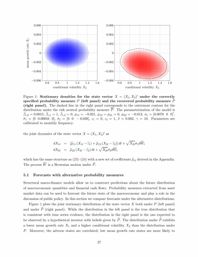
Figure 1: Stationary densities for the state vector X = (X1,X2)′ under the correctly
specified probability measure P (left panel) and the recovered probability measure P(right panel). The dashed line in the right panel corresponds to the outermost contour for thedistribution under the risk neutral probability measure P . The parameterization of the model isβc,0 = 0.0015, βc,1 = 1, βc,2 = 0, µ11 = −0.021, µ12 = µ21 = 0, µ22 = −0.013, αc = [0.0078 0 0]′,σ1 = [0 0.00034 0], σ2 = [0 0 − 0.038], ι1 = 0, ι2 = 1, δ = 0.002, γ = 10. Parameters arecalibrated to monthly frequency.
the joint dynamics of the state vector X = (X1,X2)′ as
dX1t = [µ11 (X1t − ι1) + µ12 (X2t − ι2)] dt+√X2tσ1dWt
dX2t = µ22 (X2t − ι2) dt+√X2tσ2dWt
which has the same structure as (23)–(24) with a new set of coefficients µij derived in the Appendix.
The process W is a Brownian motion under P .
5.1 Forecasts with alternative probability measures
Structural macro-finance models allow us to construct predictions about the future distribution
of macroeconomic quantities and financial cash flows. Probability measures extracted from asset
market data can be used to forecast the future state of the macroeconomy and play a role in the
discussion of public policy. In this section we compare forecasts under the alternative distributions.
Figure 1 plots the joint stationary distribution of the state vector X both under P (left panel)
and under P (right panel). While the distribution in the left panel is the true distribution that
is consistent with time series evidence, the distribution in the right panel is the one expected to
be observed by a hypothetical investor with beliefs given by P . The distribution under P exhibits
a lower mean growth rate X1 and a higher conditional volatility X2 than the distribution under
P . Moreover, the adverse states are correlated; low mean growth rate states are more likely to
27

0 20 40 60 80 1000
0.02
0.04
0.06
maturity (quarters)
consumption
yield
tomaturity
0 20 40 60 80 1000
0.02
0.04
0.06
maturity (quarters)
bon
dyield
tomaturity
Figure 2: Yields under the true and recovered probability measure. The graphs show theannualized yields on cash flows corresponding to the aggregate consumption process (left panel)and on bonds (right panel) with different maturities. The blue bands with solid lines correspond tothe distribution under P , while the red bands with dashed lines to the distribution under P . Thelines represent quartiles of the distribution. The parameterization is as in Figure 1.
occur jointly with high volatility states. Bidder and Smith (2013) document similar distortions in
a model with robustness concerns using the martingale S from equation (26).
The black dashed line in the right panel of Figure 1 gives the outermost contour line for the
joint density under the risk neutral dynamics. The distribution under the risk neutral probability
is remarkably similar to the P state probabilities and both are very different from the physical
probabilities.
The similarity between the probability measures P and P emerges because the martingale
component is known to dominate the behavior of the stochastic discount factor. See Hansen (2012)
and Backus et al. (2014) for evidence to this effect. Consider the extreme case in which the
stochastic discount factor implies that the Perron–Frobenius eigenfunction is constant and the
associated martingale implies that under the probability measure P the process X is ergodic. In
this case P = P , the short-term interest rate is constant over time and the term structure is flat.
While these term structure implications are not literally true for our parameterized recursive utility
model, the martingale component is sufficiently dominant to imply that risk adjustments embedded
P and P are very similar.
5.2 Asset pricing implications
The probability measures P and P have substantially different implications for yields and holding
period returns. In Section 4, we showed that under P , yields on risky cash flows in excess of the
riskless benchmark converge to zero as the maturity of these cash flows increases.
The left panel in Figure 2 plots the yields (20) on a payoff that equals aggregate consumption at t
as a function of t. The solid lines depict the quartiles of the yield distribution yt[C](x) corresponding
to the stationary distribution of X0 = x computed under P . The dashed lines represent the yields
28

yt[C](x) inferred by an investor who uses the recovered measure P to compute expected payoffs; but
the distribution of these yields is plotted under the correct probability measure P for the current
state X0 = x.
Because the consumption process is negatively correlated with the martingale H, the yields
computed under P are downward biased relative to P . This is necessarily true by construction
for long maturities as we show in Section 4.2, but is also true throughout the term structure. By
construction, the probability measure associated with the Perron–Frobenius martingale component
eliminates risk adjustments associated with the cash flows from aggregate consumption at long
horizons. For this example this long-term risk neutral measure accounts for virtually the whole risk
premium (in excess of the maturity-matched bond) associated with the cash flows from aggregate
consumption at all investment horizons.
6 Fundamental identification question
We now turn to an identification question. Suppose we observe Arrow prices for alternative realiza-
tions of the Markov state. Can we recover subjective beliefs? As we have already observed, asset
prices as depicted by equation (13) depend simultaneously on stochastic discount factor processes
and on investor beliefs. A stochastic discount factor process is thus only well defined for a given
probability. If we happen to misspecify investor beliefs, this misspecification can be offset by al-
tering the stochastic discount factor. This ability to offset a belief distortion poses a fundamental
challenge to the identification of subjective beliefs. In this section we formalize this identification
problem, and we consider potential restrictions on the stochastic discount factors that can solve
this challenge.
Definition 6.1. The pair (S,P ) explains asset prices if equation (13) gives the date zero price of
any bounded, Ft measurable claim Φt payable at any time t ∈ T .
Consider now a multiplicative martingale H satisfying Condition 2.2 and the associated prob-
ability measure PH defined through (15). Similarly let S be a multiplicative functional satisfying
Condition 2.2 and initialized at S0 = 1. We define:
SH = SH0
H. (27)
The following proposition is immediate:
Proposition 6.2. Suppose H is a martingale satisfying Condition 2.2 with E (H0) = 1 and S
satisfies Condition 2.2 with S0 = 1. If the pair (S,P ) explains asset prices then the pair (SH , PH)
also explains asset prices. Moreover, SH satisfies Condition 2.2 and SH0 = 1.
This proposition captures the notion that stochastic discount factors are only well-defined for
a given probability distribution. When we change the probability distribution, we typically must
change the stochastic discount factor to represent the same asset prices. Let H1 and H2 be
29

two positive martingales that satisfy Condition 2.2 with E(H1
0
)= E
(H2
0
)= 1. Construct the
corresponding stochastic discount factors using formula (27). Then we cannot distinguish the
potential subjective probabilities implied by H1 from those implied by H2 from Arrow prices alone.
There is a pervasive identification problem. To achieve identification of investor beliefs, either we
have to restrict the stochastic discount factor process S or we have to restrict the probability
distribution used to represent the valuation operators Πτ,t for τ ≤ t ∈ T .There are multiple ways we might address this lack of identification. First, we might impose
rational expectations, observe time series data, and let the Law of Large Numbers for stationary
distributions determine the probabilities. Then observations for a complete set of Arrow securities
allow us to identify S.18
Alternatively, we may restrict the stochastic discount factor process further. For instance, risk-
neutral pricing restricts the stochastic discount factor to be predetermined or locally predictable.
Thus for a discrete-time specification:
log St+1 − log St = log[q(Xt)]
where q(Xt) is the price of one-period discount bond. When this restriction is used, typically there
is no claim that the resulting probability distribution is the same as that used by investors.
A different restriction imposes a special structure on S:
Condition 6.3. Let
St = exp(−δt)m(Xt)
m(X0)
for some positive function m and some real number δ.
Ross (2015) proved an identification result under Condition 6.3 when the dynamics of X are driven
by a finite-state Markov chain as in Section 1. A strengthening of Condition 6.3 is sufficient to
guarantee that Arrow prices identify the stochastic discount factor and a probability distribution
associated with that discount factor in the more general framework introduced in Section 2.
Proposition 6.4. Suppose (S,P ) explains asset prices. Let H be a positive multiplicative martin-
gale such that (SH , PH) also explains asset prices and X is stationary and ergodic under PH . If
SH also satisfies Condition 6.3, then H is uniquely determined.
Thus if S satisfies Condition 6.3, it is the unique SH identified by this proposition, and PH identifies
the subjective beliefs P of investors. The proof of this result follows directly from our previous
analysis. Let
e =1
m
18See Hansen and Richard (1987) for an initial discussion of the stochastic discount factors and the Law of LargeNumbers, and see Hansen and Singleton (1982) for an econometric approach that imposes a parametric structure onthe stochastic discount factor and avoids assuming that the analyst has access to data on the complete set of Arrowsecurities.
30

and η = −δ. This choice of (e, η) solves the Perron–Frobenius Problem 3.1. The resulting mar-
tingale H leaves the process X as stationary and ergodic. The conclusion follows directly from
Assumption 2.1 and the uniqueness of the solution to Problem 3.1 established in Proposition 3.3.19
Recall from Section 3 that in general the P probability measure absorbs the long-term risk risk
adjustment. An immediate implication of Proposition 6.4 is that Condition 6.3 makes the long-
term risk-return tradeoff degenerate. Equivalently, the subjective discount factor process has only a
degenerate martingale component since the candidate probability measure for depicting subjective
beliefs is P = P .
7 Additional state vector
Proposition 3.3 shows how to identify a martingale associated with the Perron–Frobenius problem.
As our examples show, this martingale is, in general, non-trivial. As a consequence, the “recovered”
probability measure differs from the subjective probability measure. Perhaps the problem is that
we limit the choice of eigenfunctions too much, by assuming they depend only on the state vector
Xt, and not on Yt. As we show, relaxing this restriction on the eigenfunction could allow for the
subjective probability to correspond to one solution to the eigenfunction problem, but we may lose
identification even if we impose ergodicity on X and stationary and ergodic increments on Y .
We also examine what happens when Y is highly persistent but stationary or stationary around
a trend line. We study this phenomenon by exploring what happens when we approximate a
process with stationary increments using highly persistent stationary processes. We argue that, in
general, the lack of identification of the limit (stationary increments) process makes it likely that
the highly persistent approximations have many approximate solutions to the Perron–Frobenius
problem. This phenomenon makes the practical construction of solutions to the Perron–Frobenius
problem challenging when it is hard to distinguish a stationary process from one with stationary
increments.20 On a more positive note, we show that when we specify a priori a multiplicative
process that has the same martingale component as the stochastic discount factor, we may recover
subjective beliefs from Arrow prices.
19In a continuous-time Brownian information setup, alternative conditions on the boundary behavior of the un-derlying Markov process may also uniquely identify a probability measure. These conditions utilize linkages of thePerron–Frobenius Theorem to the Sturm–Liouville problem in the theory of second-order differential equations. Carrand Yu (2012) and Dubynskiy and Goldstein (2013) impose conditions on reflecting boundaries, while Walden (2014)analyzes natural boundaries. While technical conditions like these may deliver a unique solution, they do not resolvethe fundamental identification problem once we relax Condition 6.3.
20Walden (2014) documents similar challenges using numerical calculations in both finite- and continuous-stateapproximations.
31

7.1 Perron–Frobenius revisited
We illustrate the consequences of enlarging the state space in discrete time. Similar considerations
would hold in continuous time. Recall the joint Markov process:
Xt+1 = φx(Xt,∆Wt+1)
Yt+1 − Yt = φy(Xt,∆Wt+1).
Up until now, we have only allowed for eigenfunctions that depend on Xt, but not Yt. We now
entertain eigenfunctions that depend on (Xt, Yt) when solving the Perron–Frobenius problem. Thus
we now solve:
E
[St+1
Stε(Xt+1, Yt+1) | Xt = x, Yt = y
]= exp(η)ε(x, y).
Our previous solution remains a solution to this equation, but there may be many others. To see
why, notice that
exp (ζ · Y )
is a multiplicative functional for alternative choices of the vector ζ. For each choice ζ solve
E
[St+1
Stexp [ζ · g(Xt,∆Wt+1)] eζ(Xt+1) | Xt = x
]= exp (ηζ) eζ(x).
As a direct implication of this equation,
E
[St+1
Stexp (ζ · Yt+1) eζ(Xt+1) | Xt = x, Yt = y
]= exp (ηζ) exp (ζ · y) eζ(x).
and hence we set
ε(x, y) = exp (ζ · y) eζ(x).
For each ζ we could select a solution (should it exist) for which the implied probability measure
leaves the state vector process X ergodic and thus Y has stationary and ergodic increments. But
notice that we have constructed a family of solutions indexed by ζ. While we do not establish
existence, the approaches for doing so remain the same as S exp(ζ · Y ) is itself a multiplicative
functional. Thus, augmenting the state vector to include the stationary increment process Y
introduces more solutions to the eigenfunction problem, raising the challenge of how to select a
particular solution among this family of solutions.
This broader construction of an eigenfunction is of particular interest when the following con-
dition is satisfied.
Condition 7.1. Let
St = exp(−δt
)exp
[ζ · (Yt − Y0)
] [ m(Xt)
m(X0)
]
for some choice of parameters δ and ζ and some positive function m of the state vector Xt.
32

For instance when Yt = logCt, Assumption 7.1 requires a power utility function perhaps modified
by a function of the state vector Xt, that could measure “habit persistence.” Given Condition 7.1,
one of the potential Perron–Frobenius eigenfunctions could be used to reveal the subjective prob-
abilities, but we would still be left with the problem in identifying ζ. Even with the specificity
of Condition 7.1, there is typically a continuum of solutions to the Perron–Frobenius problem.
Changing ζ will typically alter the growth rates of the components of Y , thus prior restrictions or
other information on the subjective rate of growth could be used in conjunction with Arrow prices
in a productive way to achieve identification.
7.2 Stationary approximation
Highly persistent stationary processes are hard to distinguish from processes with stationary in-
crements. While we find it unattractive to exclude a rich class of models that specify stochastic
growth, a possible challenge to this view is to argue that model builders should focus instead on
stationary Markov models that are highly persistent. In this subsection we suggest that such highly
persistent Markov models also present challenges in actual implementation.
We now study a sequence of models that reflect this challenge. For simplicity suppose that Y is
a scalar process. The multivariate counterpart adds notation but not insight. Consider a sequence
of stationary, ergodic Markov models indexed by j:
Xt+1 = φx(Xt,∆Wt+1)
Yt+1 − Yt = ϕy(−ρjYt,Xt,∆Wt+1)
where ρj > 0 converges to zero. In the limit
Yt+1 − Yt = ϕy(0,Xt,∆Wt+1) = φy(Xt,∆Wt+1).
For instance, ϕy could be affine in its first argument:
ϕy(−ρjYt,Xt,∆Wt+1) = −ρjYt + φy(Xt,∆Wt+1).
We impose the following counterpart to Condition 6.3.
Condition 7.2. Let
St = exp(−δt) m(Xt, Yt)
m(X0, Y0)
for some positive function m and some real number δ.
For each j < ∞, Proposition 6.4 guarantees that the Perron–Frobenius problem has a unique
solution ε(x, y) = 1/m(x, y) that preserves the ergodicity of (X,Y ). For the limit problem, Condi-
tion 7.2 is not sufficient to guarantee that S is a multiplicative functional satisfying Condition 2.2.
Even after adding Condition 7.1, as we have already argued, there is typically a continuum of solu-
tions to the Perron–Frobenius problem for the limiting ρ∞ = 0 problem. This makes approximation
33

challenging as ρj becomes close to zero. The other solutions we described in subsection 7.1 above
become “approximate” solutions when ρj is close to zero.
The formal sense of approximation will matter. Strictly speaking there is no long-term growth
in Y along the sequence even though the limit process has growth. Consider the perspective of a
researcher who uses standard statistical criteria of approximation that target transition dynamics.
A highly persistent stochastic process will have growth episodes, and thus it is challenging to tell
such a process from one for which ∆Y has a positive unconditional mean using standard statistical
criteria of approximation that target transition dynamics. To analyze this further would require a
more formal discussion of the approximation which is beyond the scope of this paper.
While this sequence excludes trend growth, the argument could be extended by including a
trend line whereby
Y ∗
t = Yt + νt
and date t Arrow contracts are written terms of (Y ∗
t+1,Xt+1) or (Y∗
t+1 − Y ∗
t ,Xt+1). Then
Y ∗
t+1 − Y ∗
t = Yt+1 − Yt + ν.
We suppose that our Markov specification of pricing is given in terms of (Yt+1,Xt). If ν is known
to both the analyst and to investors inside the model, our previous analysis applies. Alternatively,
ν could be revealed by the time inhomogeneity in the Arrow prices as a function of the current
state. Either way, the computational challenges we describe previously would persist.
7.3 Structured recovery
We now explore a different generalization of Condition 6.3 that also delivers a recovery of subjective
probabilities.
Condition 7.3. The stochastic discount factor process S satisfies
St = exp(−δt)(Y rt
Y r0
)[m(Xt)
m(X0)
]
for some pre-specified multiplicative functional Y r satisfying Condition 2.2.
The pre-specified process Y r captures the long-term risk return tradeoff, and the stochastic
discount factor process S will have the same martingale component as Y r. The reciprocal of a
positive multiplicative functional is itself a multiplicative functional. We may restrict the extended
Perron–Frobenius eigenfunction to be of the form
(yr)−1 e(x).
Once we pre-specify Y r, as in Proposition 6.4, m and δ can be inferred from the Arrow prices.
Obtaining uniqueness in these circumstances amounts to postulating a process that contains the
martingale component to consumption. Given knowledge of Y r, we may again omit the more
34

general vector y from the argument of the eigenfunction in the Perron–Frobenius calculation. The
Arrow prices then reveal the probabilities.
Bansal and Lehmann (1997) and Hansen (2012) note that in many examples the multiplicative
functional Y r could come from a reference model with a direct interpretation. For instance, many
models of habit persistence, both internal and external have a stochastic discount factor that can
be depicted as
St+1
St= exp(−δ) exp [−γ(logCt+1 − logCt)]
m(Xt+1)
m(Xt)
where 1− γ is used in the power specification for per period utility and the argument of this utility
function depends on a private or social “habit stock”. For this example to be applicable we take
log Y rt = −γ logCt
for a known value of γ. The function m of the Markov state captures the impact of the implied
non-separability over time in preferences.21 Alternatively, Hansen and Scheinkman (2014) suggest
that m can be viewed as a transient misspecification of an underlying asset pricing model-based
stochastic discount factor process Y r.
8 Measuring the martingale component
In this section we consider methods for extracting evidence from asset market data about the
magnitude of the martingale component in the stochastic discount factor process. We provide a
unifying discussion of the literature and by so doing we add to the existing methods. This opens
the door to new avenues for empirical research.
The existence of the martingale has two interpretations. Under one interpretation, the assump-
tion of rational expectations allows us to assess the importance of long-term risk adjustments for
stochastically growing cash flows. Under a second interpretation it measures the statistical discrep-
ancy between subjective beliefs and the actual stochastic evolution of the state variables. For this
second interpretation to be valid, we exclude a martingale component in the stochastic discount
factor process of the subjective probability model.
8.1 Quantifying the martingale component
Statistical measures of discrepancy are often constructed using conveniently chosen convex func-
tions. Consider functions φθ defined on the positive real numbers as:
φθ(r) =1
θ(1 + θ)
[(r)1+θ − 1
]
21If the habit persistence model is fully parameterized, then given the probabilities one could solve for m asfunction of these parameters by computing the implied intertemporal marginal rates of substitution. This would leadto over-identifying restrictions.
35

for alternative choices of the parameter θ. By design φθ(1) = 0 and φ′′θ(1) = 1. The function φθ
remains well defined for θ = 0 and θ = −1 by taking pointwise limits in r as θ approaches these
two values. Thus φ0(r) = r log r and φ−1(r) = − log r. The functions φθ are used to construct
discrepancy measures between probability densities as in the work of Cressie and Read (1984).
We are interested in such measures as a way to quantify the martingale component to stochastic
discount factors. Recall that
E
[Ht+1
Ht
| Xt = x
]= 1
and that Ht+1/Ht defines a conditional density of the P distribution relative to the P distribution.
This leads us to apply the discrepancy measures to Ht+1/Ht.
Since φθ is strictly convex and φθ(1) = 0, from Jensen’s inequality:
E
[φθ
(Ht+1
Ht
)| Xt = x
]≥ 0,
with equality only when Ht+1/Ht is identically one. There are three special cases that receive
particular attention.
(i) θ = 1 in which case the implied measure of discrepancy is equal to one-half times the condi-
tional variance of Ht+1/Ht;
(ii) θ = 0 in which case the implied measure of discrepancy is based on conditional relative
entropy:
E[(Ht+1/Ht
)(log Ht+1 − log Ht
)| Xt = x
]
which is the expected log-likelihood under the P probability measure.
(iii) θ = −1 in which case the discrepancy measure is:
−E[log Ht+1 − log Ht | Xt = x
]
which is the negative of the expected log-likelihood under the original probability measure.
We consider two uses of these discrepancy measures.
8.2 Incomplete asset market data
Constructing the full range of Arrow prices for alternative states can be challenging, if not impos-
sible, in practice. For this reason it is of interest to study empirically what can be learned about
stochastic discount factor processes without using an explicit asset pricing model and without using
a complete set of prices of Arrow securities.
We build on the approach initiated by Hansen and Jagannathan (1991) aimed at nonparametric
characterizations of stochastic discount factors without using a full set of Arrow prices. While full
36

identification is not possible, data from financial markets remain informative. We draw on the
pedagogically useful characterization of Almeida and Garcia (2013) and Hansen (2014), but adapt
it to misspecified beliefs along the lines suggested in Ghosh et al. (2012) and Hansen (2014). In so
doing we build on a key insight of Kazemi (1992) and Alvarez and Jermann (2005).
We describe how to compute lower bounds for these discrepancy measures. We are led to the
study of lower bounds because we prefer not to compel an econometrician to use a full array of
Arrow prices. Let Yt+1 be a vector of asset payoffs and Qt the corresponding vector of prices. Recall
the formula for the holding period return on the long term bond
R∞
t,t+1 = exp(−η)e(Xt+1)
e(Xt),
which implies that
St+1
St=
(Ht+1
Ht
)(1
R∞
t,t+1
).
As in Alvarez and Jermann (2005) and Bakshi and Chabi-Yo (2012), suppose that the limiting
holding-period return R∞
t,t+1 can be well approximated. In this case, one could test directly for the
absence of the martingale component by assessing whether
E
[(1
R∞
t,t+1
)(Yt+1)
′ | Xt = x
]= (Qt)
′ .
More generally, we express the pricing restrictions as
E
[(Ht+1
Ht
)(1
R∞
t,t+1
)(Yt+1)
′ | Xt = x
]= (Qt)
′ ,
where H is now treated as unobservable to an econometrician. To bound a discrepancy measure,
let a random variable Jt+1 be a potential specification for the martingale increment:
Jt+1 =Ht+1
Ht
.
Solve
λθ(x) = infJt+1>0
E [φθ (Jt+1) | Xt = x]
subject to the linear constraints:
E [Jt+1 | Xt = x]− 1 = 0
E
[Jt+1
(1
R∞
t,t+1
)(Yt+1)
′ | Xt = x
]− (Qt)
′ = 0.
A strictly positive λθ(x) implies a nontrivial martingale component to the stochastic discount
37

factor.22
To compute λθ in practice requires that we estimate conditional distributions. There is an
unconditional counterpart to these calculations obtained by solving:
λθ = infJt+1>0
Eφθ(Jt+1) (28)
subject to:
E [Jt+1]− 1 = 0
E
[Jt+1
(1
R∞
t,t+1
)(Yt+1)
′ − (Qt)′
]= 0. (29)
This bound, while more tractable, is weaker in the sense that λθ ≤ Eλθ(Xt). To guarantee a
solution to optimization problem (28) it is sometimes convenient to include random variables Jt+1
that are zero with positive probability. Since the aim is to produce bounds, this augmentation can
be justified for mathematical and computational convenience. Although this problem optimizes over
an infinite-dimensional family of random variables Jt+1, the dual problem that optimizes over the
Lagrange multipliers associated with the pricing constraint (29) is often quite tractable. See Hansen
et al. (1995) and the literature on implementing generalized empirical likelihood methods for further
discussion.23 Alvarez and Jermann (2005) apply these methods to produce the corresponding
bounds for the martingale component of the stochastic discount factor process. While neither
paper computes sharp bounds of the type characterized here, both Alvarez and Jermann (2005)
and Bakshi and Chabi-Yo (2012) provide empirical evidence in support of a substantial martingale
component to the stochastic discount factor process using a very similar approach.24
8.3 Arrow prices reconsidered
In Section 7.1, we provide an extended version of the Perron–Frobenius problem to allow for
economies in which there are long-term risk adjustments in valuation. As a result of this extension,
we obtain a parameterized family of solutions even when we observe the full array of Arrow prices.
Recall that a multiplicative martingale is associated with each solution to the Perron–Frobenius
problem. One possibility is to select the parameter for which the implied subjective beliefs are
as close as possible to the actual data generating process using one of the measures of statistical
22A simple computation shows that for the continuous-time diffusion case the discrepancies equal one-half the localvariance of log H, for all values of θ.
23For the case in which θ = 1, Hansen and Jagannathan (1991) study a mathematically equivalent problem byconstructing volatility bounds for stochastic discount factors and deduce quasi-analytical formulas for the solutionobtained when ignoring the restriction that stochastic discount factors should be nonnegative. Bakshi and Chabi-Yo(2012) apply the latter methods to obtain θ = 1 bounds (volatility bounds) for the martingale component of thestochastic discount factor process. Similarly, Bansal and Lehmann (1997) study bounds on the stochastic discountfactor process for the case in which θ = −1 and show the connection with a maximum growth rate portfolio.
24Bakshi and Chabi-Yo (2012) summarize results from both papers in their Table 1 and contrast differences in theθ = 1 and θ = −1 discrepancy measures.
38

discrepancy that we describe in Section 8.1.
There are precursors to such an approach in the literature. For instance, Stutzer (1996) uses
a θ = 0 relative entropy measure of statistical discrepancy to study comparisons of risk neutral
distributions and in effect Arrow prices to empirical counterparts formed from the actual data
generation. Also, Chen et al. (2014) and Christensen (2014) suggest Perron–Frobenius methods
for semiparametric identification of stochastic discount factor models under rational expectations,
extending the approach of Hansen and Singleton (1982). Aıt-Sahalia and Lo (2000) apply a formula
from Breeden and Litzenberger (1978) to infer risk neutral densities and actual densities using
nonparametric statistical methods for low-dimensional Markov state environments.25 Insights from
this research may further help in crafting an approach to actual implementation that can be formally
justified.
9 Conclusion
Perron–Frobenius Theory applied to Arrow prices identifies a martingale component to the market-
determined stochastic discount factor process. This martingale component defines a distorted
probability measure that absorbs long-term risk adjustments, in the same spirit as the risk neutral
probability measure absorbs one-period risk adjustments. We call this measure the long-term risk
neutral measure.
One identifying assumption, featured by Ross (2015), assumes that this martingale component
is identical to one under the subjective beliefs of the investors. In this case, the probability measure
recovered by the Perron–Frobenius Theory coincides with the subjective probability measure. If,
however, the stochastic discount factor process includes a martingale component, then the use of
the Perron–Frobenius eigenvalue and function recovers a long-term risk neutral pricing measure
that is distorted by this martingale component.26 By expanding the space of functions used in
seeking a solution to the Perron–Frobenius problem, we avoid assuming that long-term risk return
tradeoffs are degenerate under subjective beliefs, but we inherit an identification problem. There
is typically a whole family of solutions with little guidance as to which solution should be selected
by an analyst.
Many structural models of asset pricing that are motivated by empirical evidence have non-
trivial martingale components in the stochastic discount factors. These martingales characterize
what probability is actually recovered by the application of Perron–Frobenius Theory. We illustrate
this outcome in one example with long-run risk components to the macroeconomy and with investors
that have non-separable recursive preferences. We also provide a unifying discussion of the empirical
25See also Garcia et al. (2010) for a recent survey of econometric methods for the study of options prices andGagliardini et al. (2011) for a discussion of the econometric impact of combining a rich set of options prices fora limited number of dates with time series evidence over many periods. This latter work also imposes rationalexpectations.
26Recent working papers by Qin and Linetsky (2014a,b) provide additional results in the continuous state space envi-ronment, with explicit connections to previous results in Hansen and Scheinkman (2009) and Hansen and Scheinkman(2014).
39
literature that derives non-parametric bounds for the magnitude of the martingale component and
that finds a quantitatively large role for this martingale component for valuation. Finally, we
suggest ways to further expand the set of testable implications in this literature and to combine
information about subjective beliefs from Arrow prices with the observed time series evolution.
In our previous work we showed how Perron–Frobenius Theory helps us understand risk-return
tradeoffs. The probability measure identified by Perron–Frobenius Theory absorbs the long-term
risk adjustments. Its naive use can distort the risk-return tradeoff in unintended ways. One might
argue, however, that the dynamics under the Perron–Frobenius probability measure are of interest
precisely because this measure adjusts for the long-term riskiness of the macroeconomy. While we
see value in using this probability measure prospectively, our analysis makes clear that the resulting
forecasts are slanted in a particular but substantively interesting way.
Finally, long-term valuation is only a component to a more systematic study of pricing implica-
tions over alternative investment horizons. Recent work by Borovicka et al. (2011) and Borovicka
et al. (2014) deduces methods that extend impulse response functions to characterize the pricing
of exposures to shocks to stochastically growing cash flows over alternative investment horizons.
40

Appendix
A Multiplicative functional
The construct of a multiplicative functional is used elsewhere in the probability literature and in Hansen
and Scheinkman (2009). Formally a multiplicative functional is a process M that is adapted to F, initialized
at M0 = 1 and, with a slight abuse of notation:
Mt(Y ) =Mτ (Y )Mt−τ (θτ (Y )). (30)
In formula (30), θτ is the shift operator that moves the time subscript of Y by τ , that is, (θτ (Y ))s = Yτ+s.
We generalize this construct by building an extended multiplicative functional. The process M is an
extended multiplicative functional ifM0 is a strictly positive (Borel measurable) function ofX0 and Mt/M0 :
t ∈ T is a multiplicative functional. This allows the process M to be initialized at M0 different from unity.
In this paper we drop the use of the term extended for pedagogical convenience.
B Perron–Frobenius Theory
Proof of Proposition 3.3. Suppose there are two solutions η, e and η, e. Hence:
exp(ηt)Ht
H0
e(X0)
e(Xt)= exp(ηt)
Ht
H0
e(X0)
e(Xt)
or if k(xt) =e(Xt)e(Xt)
> 0, and η = η − η
exp(−ηt) Ht
H0
k(Xt)
k(X0)=Ht
H0
,
Calculating expected values in both sides and using the fact that H is a martingale we obtain that for H = H
EH [k(Xt) | X0 = x] = exp(ηt)k(x). (31)
In what follows we consider the discrete-time case. The continuous-time case uses an identical approach,
with the obvious changes. First note that for a bounded function f the Law of Large Numbers implies that
limN→∞
1
N
N∑
t=1
EH [f(Xt) | X0 = x] = EH [f(X0)] (32)
for H = H and H = H. Consider three cases. First suppose that η < 0. Set
k(x) = min 1, k(x) > 0, for all x.
Since η < 0, the right-hand side of (31) converges to zero for each x as t→ ∞. Thus, for H = H
0 = limN→∞
1
N
N∑
t=1
EH [k(Xt) | X0 = x] ≥ limN→∞
1
N
N∑
t=1
EH[k(Xt) | X0 = x
]= EH
[k(X0)
]> 0.
Thus we have established a contradiction.
41

Next suppose that η > 0. Note that for H = H
EH
[1
k(Xt)|X0 = x
]= exp(−ηt) 1
k(x). (33)
Form
k(x) = min
1,
1
k(x)
> 0, for all x.
Since η > 0, the right-hand side of (33) converges to zero for each x as t→ ∞. Thus,
0 = limN→∞
1
N
N∑
t=1
EH
[1
k(Xt)|X0 = x
]≥ lim
N→∞
1
N
N∑
t=1
EH[k(Xt)|X0 = x
]= EH
[k(X0)
]> 0.
We have again established a contradiction.
Finally, suppose η = 0. Then again for for H = H,
EH
[1
k(Xt)|X0 = x
]=
1
k(x)
for all x. From (32):
limN→∞
1
N
N∑
t=1
EH [kn(Xt)|X0 = x] = EHkn(X0).
for kn = min1/k, n. The same equality applies to the limit as n → ∞ whereby kn is replaced by 1/k.
Consequently, EH[
1k(X0)
]= 1
k(x) for almost all x. Thus k(x) is a constant, and Ht
H0
= Ht
H0
with probability
one.
C Long-term valuation limits
First we verify that the approximation results described in Section 4.1 hold under weaker conditions than
Condition 4.1. We assume instead:
lim inft→∞
E [ψ (Xt) | X0 = x] > 0 (34)
and that
lim inft→∞
E
[ψ(Xt)
e(Xt)| X0 = x
]> 0.
Notice that these assumptions follows if for every bounded function f
limt→∞
E [f(Xt) | X0 = x] = E [f(X0)] (35)
almost surely. Meyn and Tweedie (2009) establish in Theorem 13.3.3 on page 327 that (35) holds for bounded
functions f , provided X is aperiodic and positive Harris recurrent under the measure P .
Furthermore, we assume that
E
[ψ(Xt)
e(Xt)
]<∞, E [ψ(Xt)] < +∞,
42

and that X satisfies Condition 3.2 under P . Then,
1
Nlog E [ψ (XN ) | X0 = x] ≤ 1
Nlog
(E
[N∑
t=1
ψ (Xt) |X0 = x
])
=1
NlogN +
1
Nlog
(E
[1
N
N∑
t=1
ψ (Xt) |X0 = x
]).
Result (34) implies that the lim inf on the left-hand side converges to zero. The lim sup of the left-hand side
also converges to zero. To verify this, note that the Law of Large Numbers and the resulting almost sure
convergence extend to the time-series averages of conditional expectations,
limN→∞
E
[1
N
N∑
t=1
ψ (Xt) |X0 = x
]= E [ψ (X0)]
almost surely. Hence both terms on the right-hand side of (36) converge to zero with probability one.
Consequently, lim sup on the left-hand side does as well. Given both the lim inf and lim sup on the left-hand
side of (36) to zero the left-hand side must converge to zero almost surely.
The same logic implies that
limN→∞
1
Nlog E
[ψ(XN )
e(XN )| X0 = x
]= 0,
with probability one.27
Next introduce stochastic growth into the analysis as in Section 4.2. First note that the multiplicative
functional SG satisfies Condition 2.2. Let η∗ denote the Perron–Frobenius eigenvalue using SG in place of
S when solving Problem 3.1. This entails solving:
E [StGte∗(Xt) | X0 = x] = exp (η∗t) e∗(x)
and selecting the eigenvalue-eigenfunction pair such that the implied martingale induces stationarity and
ergodicity. Imitating our calculation of yields on securities with stationary payoffs
E
(StGt
[e(Xt)
e(X0)
]| X0 = x
)= exp (tη∗)E∗
[e(Xt)e
∗(X0)
e(X0)e∗(Xt)| X0 = x
]
where E∗ is constructed using the martingale H∗ with increments:
H∗t
H∗0
= exp (−η∗)StGt
[e∗(Xt)
e∗(X0)
].
Similarly,
E (StGt | X0 = x) = exp (tη∗)E∗
([e∗(X0)
e∗(Xt)
]| X0 = x
).
Suppose that H∗ induces a probability measure under which Condition 4.1 is satisfied. In addition suppose
27For the continuous-time case, sample the Markov process at integer points in time. The process remains stationaryunder P , but is not necessarily ergodic. The Law of Large Numbers still applies but with a limit that is the expectationconditioned on invariant events. The previous argument with these modifications establishes the limiting behavior.
43

that
E∗
[e(Xt)
e∗(Xt)
]<∞, E∗
[1
e∗(Xt)
]<∞.
From Condition 4.1 we obtain,
limt→∞
1
tE∗
[e(Xt)
e∗(Xt)| X0 = x
]= 0
limt→∞
1
tlogE∗
[1
e∗(Xt)| X0 = x
]= 0.
Thus
limt→∞
1
tlogE
(StGt
[e(Xt)
e(X0)
]| X0 = x
)=
= η∗ + limt→∞
1
t[log e∗(x)) − log e(x)] + lim
t→∞
1
tE∗
[e(Xt)
e∗(Xt)| X0 = x
]= η∗,
and similarly
limt→∞
1
tlogE (StGt | X0 = x) =
= η∗ + limt→∞
1
tlog e∗(x) + lim
t→∞
1
tlogE∗
[1
e∗(Xt)| X0 = x
]= η∗.
Hence
limt→∞
yt[G](x) = −η + η∗ − η∗ = −η.
D Derivations for the model with predictable consumption dynamics
In this section, we provide derivations for the model analyzed in Section 5. We will focus on the analysis of
the Perron–Frobenius problem. A complete analysis of the model can be found in Hansen (2012) and in the
appendix in Borovicka et al. (2014).
D.1 Martingale decomposition
We solve the Perron–Frobenius problem
E [Ste (Xt) | X0 = x] = exp (ηt) e (x)
where S is a multiplicative functional parameterized by coefficients (βs(x), αs(x)). Since the problem holds
for every t, then it also holds in the limit (as long as it exists)
limtց0
1
t[E [Ste (Xt) | X0 = x]− exp (ηt) e (x)] = 0.
The limit yields the partial differential equation
Se = ηe
44

where, in the general Brownian information setup given by equations (16), the infinitesimal generator S is
given by
Se =
(βs +
1
2|αs|2
)e+ ex · (µ+ σαs) +
1
2tr [exxσσ
′] .
Equation (D.1) is therefore a second-order partial differential equation, and we are looking for a solution in
the form of a number η and a strictly positive function e. Hansen and Scheinkman (2009) show that if there
are multiple such solutions, then only the solution associated with the lowest value of η can generate ergodic
dynamics under the implied change of measure.
In the case of the long-run risk model introduced in Section 5 and parameterized by (23)–(25), we can
guess
e (x) = exp (e1x1 + e2x2)
which leads to the system of equations
η = βs,0 − βs,11ι1 − βs,12ι2 − e1 (µ11ι1 + µ12ι2)− e2µ22ι2
0 = βs,11 + µ11e1
0 = βs,12 +1
2|αs|2 + e1 (µ12 + σ1αs) +
1
2e21 |σ1|
2+ e2 (µ22 + σ2αs + e1σ1σ
′2) +
1
2(e2)
2 |σ2|2 .
The coefficients βs,· and αs will be determined below. The last equation is a quadratic equation for e2 and
we choose the solution for e2 that leads to the smaller value of η. From the decomposition
St = exp (ηt)e (X0)
e (Xt)
Ht
H0
we can extract the martingale H:
d log Ht = d logSt − ηdt+ d log e (Xt)
and thusdHt
Ht
=√X2t (αs + σ′
1e1 + σ′2e2) · dWt=
√X2tαh · dWt.
This martingale implies a change of measure such that W defined as
dWt = −√X2tαhdt+ dWt
is a Brownian motion under the new measure P . Under the change of measure implied by H , we can write
the joint dynamics of the model as
dX1t = [µ11 (X1t − ι1) + µ12 (X2t − ι2)] dt+√X2tσ1dWt
dX2t = µ22 (X2t − ι2) dt+√X2tσ2dWt
where
µ11 = µ11 µ12 = µ12 + σ1αh µ22 = µ22 + σ2αh
ι2 =µ22
µ22ι2 ι1 = ι1 + (µ11)
−1 (µ12ι2 − µ12ι2) .
45

Similarly, every multiplicative functional M with parameters given by (25) can be rewritten as
d logMt =[β0 + β11 (X1t − ι1) + β12 (X2t − ι2)
]dt+
√X2tα · dWt
where
β0 = β0 + β11 (ι1 − ι1) + β12 (ι2 − ι2) + (α · αh) ι2
β11 = β11 β12 = β12 + α · αh.
D.2 Value function and stochastic discount factor for recursive utility
We choose a convenient choice for representing continuous values. Similar to the discussion in Schroder and
Skiadas (1999), we use the counterpart to discounted expected logarithmic utility.
d logVt = µv,tdt+ σv,t · dWt.
The local evolution satisfies:
µv,t = δ logVt − δ logCt −1− γ
2|σv,t|2 (37)
When γ = 1 this collapses to the discounted expected utility recursion.
Let
logVt = logCt + v(Xt)
and guess that
v (x) = v0 + v1 · x1 + v2x2.
We compute µv,t by applying the infinitesimal generator to logC + v(X). In addition,
σv,t = αc (Xt) + σ (Xt)′ ∂
∂xv (Xt) .
Substituting into (37) leads to a set of algebraic equations
δv0 = βc,0 − ι1(βc,1 + µ11v1
)− ι2
(βc,2 + µ12v1 + µ22v2
)
δv1 = βc,1 + µ11v1
δv2 = βc,2 + µ12v1 + µ22v2 +1
2(1− γ) |αc + σ′
1v1 + σ′2v2|
2
which can be solved for the coefficients vi. The third equation is a quadratic equation for v2 that has a real
solution if and only if
D =[µ22 − δ + (1− γ) (αc + σ′
1v1)′σ′2
]2−
−2 (1− γ) |σ2|2(βc,2 + µ12v1 +
1
2(1− γ) |αc + σ′
1v1|2)
≥ 0.
In particular, the solution will typically not exist for large values of γ. If the solution exists, it is given by
v2 =−[µ22 − δ + (1− γ) (αc + σ′
1v1)′σ′2
]±√D
(1− γ) |σ′2|
2
46
The solution with the minus sign is the one that interests us.
The resulting stochastic discount factor has two components. One component is the intertemporal
marginal rate of substitution for discounted log utility and the other is a martingale constructed from the
continuation value
d logSt = −δdt− d logCt + d logH∗t
where H∗ is a martingale given by
dH∗t
H∗t
=√X2,t (1− γ) (αc + σ′
1v1 + σ′2v2)
′dWt.
This determines the coefficients (βs(x), αs(x)) of the stochastic discount factor.
When we choose the ‘minus’ solution in equation (D.2), then S implies a change of measure that preserves
ergodicity. Notice that while H∗ is a martingale, it is distinct from Ht/H0 as long as the consumption process
itself contains a nontrivial martingale component.
D.3 Conditional expectations of multiplicative functionals
In order to compute asset prices and their expected returns, we need to compute conditional expectations
of multiplicative functionals M parameterized by (23)–(25). These conditional expectations are given by
E [Mt | X0 = x] = exp [θ0(t) + θ1(t) · x1 + θ2(t)x2] ,
where parameters θi(t) satisfy a system of ordinary differential equations derived in Hansen (2012) and in
the appendix of Borovicka et al. (2014).
47
References
Aıt-Sahalia, Yacine and Andrew Lo. 2000. Nonparametric risk management and implied risk aver-
sion. Journal of Econometrics 94 (1-2):9–51.
Almeida, Caio and Rene Garcia. 2013. Robust Economic Implications of Nonlinear Pricing Kernels.
Alvarez, Fernando and Urban J. Jermann. 2005. Using Asset Prices to Measure the Persistence of
the Marginal Utility of Wealth. Econometrica 73 (6):1977–2016.
Anderson, Evan W., Lars Peter Hansen, and Thomas J. Sargent. 2003. A Quartet of Semigroups for
Model Specification, Robustness, Prices of Risk, and Model Detection. Journal of the European
Economic Association 1 (1):68–123.
Backus, David K., Allan W. Gregory, and Stanley E. Zin. 1989. Risk Premiums in the Term
Structure : Evidence from Artificial Economies. Journal of Monetary Economics 24 (3):371–399.
Backus, David K., Mikhail Chernov, and Stanley E. Zin. 2014. Sources of Entropy in Representative
Agent Models. The Journal of Finance 59 (1):51–99.
Bakshi, Gurdip and Fousseni Chabi-Yo. 2012. Variance Bounds on the Permanent and Transitory
Components of Stochastic Discount Factors. Journal of Financial Economics 105 (1):191–208.
Bansal, Ravi and Bruce N. Lehmann. 1994. Addendum to ‘Growth-Optimal Portfolio Restrictions
on Asset Pricing Models’. Unpublished manuscript.
———. 1997. Growth-Optimal Portfolio Restrictions on Asset Pricing Models. Macroeconomic
Dynamics 1 (2):333–354.
Bansal, Ravi and Amir Yaron. 2004. Risks for the Long Run: A Potential Resolution of Asset
Pricing Puzzles. Journal of Finance 59 (4):1481–1509.
Bidder, Rhys and Matthew E. Smith. 2013. Doubts and Variability: A Robust Perspective on
Exotic Consumption Series. Federal Reserve Bank of San Francisco Working Paper 2013–28.
Borovicka, Jaroslav, Lars Peter Hansen, Mark Hendricks, and Jose A. Scheinkman. 2011. Risk
Price Dynamics. Journal of Financial Econometrics 9 (1):3–65.
Borovicka, Jaroslav, Lars Peter Hansen, and Jose A. Scheinkman. 2014. Shock Elasticities and
Impulse Responses. Mathematics and Financial Economics 8 (4):333–354.
Breeden, Douglas T. and Robert H. Litzenberger. 1978. Prices of State-Contingent Claims Implicit
in Option Prices. The Journal of Business 51 (4):621–51.
Breiman, Leo. 1982. Probability. Volume 7 of Classics in Applied Mathematics. Philadelphia, PA:
Society for Industrial and Applied Mathematics (SIAM).
48

Carr, Peter and Jiming Yu. 2012. Risk, Return and Ross Recovery. The Journal of Derivatives
20 (1):38–59.
Chen, Xiaohong, Victor Chernozhukov, Sokbae Lee, and Whitney K. Newey. 2014. Local Identifi-
cation of Nonparametric and Semiparametric Models. Econometrica 82 (2):785–809.
Christensen, Timothy M. 2014. Nonparametric Indentification of Positive Eigenfunctions. Econo-
metric Theory FirstView:1–21.
Cressie, Noel and Timothy R. C. Read. 1984. Multinomial Goodness-of-Fit Tests. Journal of the
Royal Statistical Society. Series B (Methodological) 46 (3):440–464.
Dubynskiy, Sergey and Robert S. Goldstein. 2013. Recovering Drifts and Preference Parameters
from Financial Derivatives.
Duffie, Darrell and Larry G. Epstein. 1992. Asset Pricing with Stochastic Differential Utility. The
Review of Financial Studies 5 (3):411–436.
Epstein, Larry G. and Stanley E. Zin. 1989. Substitution, Risk Aversion, and the Temporal Behavior
of Consumption and Asset Returns: A Theoretical Framework. Econometrica 57 (4):937–969.
Gagliardini, Patrick, Christian Gourieroux, and Eric Renault. 2011. Efficient Derivative Pricing by
the Extended Method of Moments. Econometrica 79 (4):1181–1232.
Garcia, Rene, Eric Ghysels, and Eric Renault. 2010. The Econometrics of Option Pricing. In
Handbook of Financial Econometrics: Tools and Techniques, vol. 1 of Handbooks in Finance,
edited by Lars Peter Hansen and Yacine Aıt-Sahalia, chap. 9, 479 – 552. San Diego: North-
Holland.
Ghosh, Anisha, Christian Julliard, and Alex Taylor. 2012. What is the Consumption-CAPM Miss-
ing? An Information-Theoretic Framework for the Analysis of Asset Pricing Models. Working
paper, Tepper School of Business, Carnegie Mellon University.
Hansen, Lars Peter. 2012. Dynamic Valuation Decomposition within Stochastic Economies. Econo-
metrica 80 (3):911–967. Fisher–Schultz Lecture at the European Meetings of the Econometric
Society.
———. 2014. Nobel Lecture: Uncertainty Outside and Inside Economic Models. Journal of Political
Economy 122 (5):945–987.
Hansen, Lars Peter and Ravi Jagannathan. 1991. Implications of Security Market Data for Models
of Dynamic Economies. Journal of Political Economy 99 (2):225–262.
Hansen, Lars Peter and Scott F. Richard. 1987. The Role of Conditioning Information in Deducing
Testable Restrictions Implied by Dynamic Asset Pricing Models. Econometrica 55 (3):587–613.
49

Hansen, Lars Peter and Jose A. Scheinkman. 2009. Long Term Risk: An Operator Approach.
Econometrica 77 (1):177–234.
———. 2014. Stochastic Compounding and Uncertain Valuation.
Hansen, Lars Peter and Kenneth J. Singleton. 1982. Generalized Instrumental Variables Estimation
of Nonlinear Rational Expectations Models. Econometrica 50 (5):1269–1286.
Hansen, Lars Peter, John Heaton, and Erzo G. J. Luttmer. 1995. Econometric Evaluation of Asset
Pricing Models. The Review of Financial Studies 8 (2):237–274.
Hansen, Lars Peter, John C. Heaton, Junghoon Lee, and Nikolai Roussanov. 2007. Intertemporal
Substitution and Risk Aversion. In Handbook of Econometrics, vol 6A, edited by James J.
Heckman and Edward E. Leamer, 3967–4056. Amsterdam: North-Holland.
Hansen, Lars Peter, John C. Heaton, and Nan Li. 2008. Consumption Strikes Back? Measuring
Long-Run Risk. Journal of Political Economy 116:260–302.
Harrison, J. Michael and David M. Kreps. 1979. Martingales and Arbitrage in Multiperiod Securities
Markets. Journal of Economic Theory 20 (3):381–408.
Hilscher, Jens, Alon Raviv, and Ricardo Reis. 2014. Inflating Away the Public Debt? Columbia
University.
Kazemi, Hossein B. 1992. An Intertemporal Model of Asset Prices in a Markov Economy with a
Limiting Stationary Distribution. Review of Financial Studies 5 (1):85–104.
Kreps, David M. and Evan L. Porteus. 1978. Temporal Resolution of Uncertainty and Dynamic
Choice Theory. Econometrica 46 (1):185–200.
Meyn, Sean P. and Richard L. Tweedie. 1993. Stability of Markovian Processes II: Continuous-Time
Processes and Sampled Chains. Advances in Applied Probability 25 (3):487–517.
———. 2009. Markov Chains and Stochastic Stability. Cambridge, United Kingdom: Cambridge
University Press.
Park, Hyungbin. 2014. Ross Recovery with Recurrent and Transient Processes.
Qin, Likuan and Vadim Linetsky. 2014a. Long Term Risk: A Martingale Approach. Mimeo,
Northwestern University.
———. 2014b. Positive Eigenfunctions of Markovian Pricing Operators: Hansen–Scheinkman Fac-
torization and Ross Recovery. Mimeo, Northwestern University.
Ross, Stephen A. 1978. A Simple Approach to the Valuation of Risky Streams. The Journal of
Business 51 (3):453–75.
50
Ross, Stephen A. 2015. The Recovery Theorem. Journal of Finance 70 (2):615–648.
Schroder, Mark and Costis Skiadas. 1999. Optimal Consumption and Portfolio Selection with
Stochastic Differential Utility. Journal of Economic Theory 89 (1):68–126.
Stutzer, Michael. 1996. A Simple Nonparametric Approach to Derivative Security Valuation. The
Journal of Finance 51 (5):1633–1652.
Walden, Johan. 2014. Recovery with Unbounded Diffusion Processes.
51