Excavator Tutorial (RFlex) - RecurDyn Technical Supportsupport.recurdyn.com/wp-content/uploads/2015/11/RFlexExcavator... · FunctionBay, Inc. hereby grants to the licensed user the

Excavator Tutorial (RFlex)

E X C A V A T O R T U T O R I A L ( R F L E X )

２

Copyright © 2016 FunctionBay, Inc. All rights reserved

User and training documentation from FunctionBay, Inc. is subjected to the copyright laws of the Republic of Korea and other countries and is provided under a license agreement that restricts copying, disclosure, and use of such documentation. FunctionBay, Inc. hereby grants to the licensed user the right to make copies in printed from of this documentation if provided on software media, but only for internal/personal use and in accordance with the license agreement under which the applicable software is licensed. Any copy made shall include the FunctionBay, Inc. copyright notice and any other proprietary notice provided by FunctionBay, Inc. This documentation may not be disclosed, transferred, modified, or reduced to any form, including electronic media, or transmitted or made publicly available by any means without the prior written consent of FunctionBay, Inc. and no authorization is granted to make copies for such purpose.

Information described herein is furnished for general information only, is subjected to change without notice, and should not be construed as a warranty or commitment by FunctionBay, Inc. FunctionBay, Inc. assumes no responsibility or liability for any errors or inaccuracies that may appear in this document.

The software described in this document is provided under written license agreement, contains valuable trade secrets and proprietary information, and is protected by the copyright laws of the Republic of Korea and other countries. UNAUTHORIZED USE OF SOFTWARE OR ITS DOCUMENTATION CAN RESULT IN CIVIL DAMAGES AND CRIMINAL PROSECUTION.

Registered Trademarks of FunctionBay, Inc. or Subsidiary

RecurDyn™ is a registered trademark of FunctionBay, Inc.

RecurDyn™/SOLVER, RecurDyn™/MODELER, RecurDyn™/PROCESSNET, RecurDyn™/AUTODESIGN,

RecurDyn™/COLINK, RecurDyn™/DURABILITY, RecurDyn™/FFLEX, RecurDyn™/RFLEX,

RecurDyn™/RFLEXGEN, RecurDyn™/LINEAR, RecurDyn™/EHD(Styer), RecurDyn™/ECFD_EHD,

RecurDyn™/CONTROL, RecurDyn™/MESHINTERFACE, RecurDyn™/PARTICLES,

RecurDyn™/PARTICLEWORKS, RecurDyn™/ETEMPLATE, RecurDyn™/BEARING, RecurDyn™/SPRING,

RecurDyn™/TIRE, RecurDyn™/TRACK_HM, RecurDyn™/TRACK_LM, RecurDyn™/CHAIN,

RecurDyn™/MTT2D, RecurDyn™/MTT3D, RecurDyn™/BELT, RecurDyn™/R2R2D, RecurDyn™/HAT,

RecurDyn™/CRANK, RecurDyn™/PISTON, RecurDyn™/VALVE, RecurDyn™/TIMINGCHAIN,

RecurDyn™/ENGINE, RecurDyn™/GEAR are trademarks of FunctionBay, Inc.

Third-Party Trademarks

Windows and Windows NT are registered trademarks of Microsoft Corporation.

ProENGINEER and ProMECHANICA are registered trademarks of PTC Corp. Unigraphics and I-DEAS are registered trademark of UGS Corp. SolidWorks is a registered trademark of SolidWorks Corp. AutoCAD is a registered trademark of Autodesk, Inc.

CADAM and CATIA are registered trademark of Dassault Systems. FLEXlm is a registered trademark of GLOBEtrotter Software, Inc. All other brand or product names are trademarks or registered trademarks of their respective holders.

Edition Note

These documents describe the release information of RecurDyn™ V8R5.


３

Table of Contents

Getting Started ................................................................................................ 4

Objective ............................................................................................................................... 4

Approach ............................................................................................................................... 4

Audience ............................................................................................................................... 5

Prerequisites ......................................................................................................................... 5

Procedures ............................................................................................................................ 6

Estimated Time to Complete ................................................................................................. 6

Opening the Initial Model ................................................................................. 7

Task Objective ...................................................................................................................... 7

Estimated Time to Complete ................................................................................................. 7

Starting RecurDyn ................................................................................................................. 8

Running an Initial Simulation with the Rigid Boom ............................................................. 10

Viewing the Results ............................................................................................................ 10

Swapping In the RFlex Body ............................................................................................... 11

Task Objective .............................................................................................. 11

Estimated Time to Complete ............................................................................................... 11

Swapping In the RecurDyn RFlex Body ............................................................................. 12

Viewing Stress Contour Plots ............................................................................................. 14

Plotting the Results ....................................................................................... 16

Task Objective .................................................................................................................... 16


Plotting the Dipper Stick’s Out-of-Plane Tilt ........................................................................ 17

RFlex Body Review and Tuning .................................................................... 20

Task Objective .................................................................................................................... 20


Examining the RFlex Body .................................................................................................. 21

Improving Simulation Performance ..................................................................................... 24

Appendix A : Creating the RecurDyn RFlex Input (RFI) File ........................ 26

Task Objective .................................................................................................................... 26

Estimated Time to Complete .............................................................................................. 26

Preparing the Nastran Bulk Data File ................................................................................. 27

Component Mode Reduction Method ................................................................................. 27

Superelement Method ......................................................................................................... 29

Appendix B : Supported FE Elements ........................................................... 32

Ansys Element Library ........................................................................................................ 33

MSC/NASTRAN Element Library ........................................................................................ 33

I-DEAS Element Library ...................................................................................................... 34


4

Getting Started

Objective

In this tutorial, you will learn how to simulate a model which has a flexible body. You will start with an existing model which has all rigid bodies, and replace one of them with a RecurDyn RFlex body. RecurDyn RFlex uses a modal approach to represent flexible bodies, by using the superposition of the body’s natural modal shapes and constraint modes at the attachment points. This approach is ideal when the flexible body has only fixed connection points to other bodies. If it has sliding or rolling contact, RecurDyn FFlex should be used, which takes a nodal (or mesh-based) approach to represent the body.

Approach

You will start with an excavator model, shown below, that includes all of the mechanical components. All the bodies in this model are rigid. The model is set up so that the excavator goes through a digging and unloading motion, with the cab rotating around the vertical axis.

You will then import a RecurDyn RFlex Input (RFI) file, which represents a flexible boom. One way to create an RFI file is by using NX Advance Simulation to mesh the boom geometry, export the simulation to a Nastran bulk data file, and then use NX Nastran to read the bulk data file and create the RFI file.

The RFI file is supplied with this tutorial. For information on how to create the RFI file from a Nastran bulk data file, see the appendix.

Chapter

1


5

Audience

This tutorial is intended for intermediate users of RecurDyn who previously learned how to create geometry, joints, and force entities. All new tasks are explained carefully.

Prerequisites

You should first work through the 3D Crank-Slider and Engine with Propeller tutorials, or the equivalent. We assume that you have a basic knowledge of physics.

You will need a license for the RFlex module of RecurDyn.


6

Procedures

The tutorial is comprised of the following procedures. The estimated time to complete each procedure is shown in the table.

Procedures Time (minutes)

Opening the Initial Model 10

Importing and Connecting the RFlex Body 20

Plotting the Results 5

Creating a RecurDyn RFlex Input (RFI) File 10

Total: 45

Estimated Time to Complete

This tutorial takes approximately 45 minutes to complete.


7

Opening the Initial Model

Task Objective

Open the initial model, run a simulation, and observe the digging/unloading motion.


10 minutes

Chapter

2


7

Starting RecurDyn

To start RecurDyn and open the initial model:

1. On your Desktop, double-click the RecurDyn icon.

2. When the Start RecurDyn dialog box appears close it because you will not be creating a new model but using an existing one.

3. From the File menu, click Open.

4. From the RFlex tutorial directory, select the file

RD_Excavator_Start.rdyn. (The file location:

<Install Dir> \Help \Tutorial \Flexible \RFlex, ask your instructor for the location of the directory if you cannot find it).

5. Click Open.

Your model should look like the following.

The boom indicated above, between the cab and the dipper stick, is the rigid body in this model which you will later model as a flexible body.


9

To save the initial model:

1. From the File menu, click Save As.

2. Save the model different directory, because you cannot simulation in tutorial directory.


9

Running an Initial Simulation with the Rigid Boom

You will now run an initial simulation of the model to understand the motion that it will go through.

To run an initial simulation:

1. From the Simulation Type group in the

Analysis tab, click Dyn/Kin.

The Dynamic/Kinematic Analysis dialog window appears.

2. Define the End Time and Step values as follows:

End Time: 3.0

Step: 200

Plot Multiplier Step Factor: 5

3. Click Simulate. The simulation will run in about 10 seconds, depending on the speed of your computer.

Viewing the Results

To view the results:

From the Animation Control group in the Analysis tab, click Play/Pause.

You should see the excavator rotate about the vertical axis, and then goes through a digging and then unloading motion. This is being driven by motion input to the revolute joint around which the cab rotates, and translational joints in the hydraulic cylinders.


11

Swapping In the RFlex Body

Task Objective

In this chapter, you will learn how to import the RFlex body representing the flexible boom. Using RFlex’s “flexible body swap” functionality, you will also replace the rigid body in the same step. You will then run a simulation with the new flexible boom body, and view a stress contour plot.


20 minutes

Chapter

3


12

Swapping In the RecurDyn RFlex Body

You will now import the RecurDyn RFlex Input (RFI) file, which represents the flexible boom. In the same step, you will replace the corresponding rigid body.

To swap in the RFlex body:

1. From the RFlex group in the Flexible tab, click Import RFI.

2. Set the Creation Method toolbar to Body.

3. In the Working window,

select the Rigid_Boom body.

4. In the RFLEX Body Import

window, to the left of the Import button, click the browse button (…).

5. Select the file named boom_tet_mesh_rfi_0.rfi, in the

RFlex tutorial directory, and click Open. (The file

location: <Install Dir> \Help \Tutorial \Flexible \RFlex, ask your instructor for the location of the directory if you cannot find it).

6. To the right of Reference Frame, select the browse

button (…).

7. In the Database window, navigate to the Ground.InertiaMarker marker (Bodies > Ground

> Markers > InertiaMarker).

8. Select Ground.InertiaMarker and drag it to the Navigation

Target window in the upper-right corner of the Working window.

Note: To successfully drag the marker to the Navigation Target window, you may have to select another database element, and then select Ground.InertiaMarker again and drag it to the Navigation Target window in a single mouse click.

9. Click OK to import the body.


13

The RFlex boom body should now have replaced the rigid boom body, as shown below (may be a different color than green). By checking in the Database window, you should notice that the rigid boom body is no longer in the model.

Important: In the next step, it is important to save the model using a different filename, as the results from the new file will be compared with the old.

10. Save the model as RD_Excavator_RFlex.rdyn.

11. Run a new simulation. This should take ~2 minutes, depending on the speed of your computer


14

Viewing Stress Contour Plots

You can now use RecurDyn to view the areas of high stress within the flexible boom as it goes through the digging/unloading motion.

To view a stress contour plot:

1. From the RFlex group in the Flexible tab, click Contour.

2. In the lower left region of the Contour Dialog, select the checkbox next to Enable Contour

View.

3. Under Contour Option, to the right of Type, select Stress.

4. Select SMISES from the list.

5. Under Min/Max Option, click the Calculation button.

This will determine the minimum and maximum stress that occurs during the simulation within the

flexible boom. The values for Min and Max should be updated as shown below.

6. Now adjust the maximum value so that the contour display will show stresses at a lower range:

Change the Type to User Defined.

Type in 200 for the Max value.

Click the checkbox next to Show Min/Max.

Click the checkbox next to User Defined Max Color.

Change Exceed Max Color to red


14

7. Click OK

8. Play the animation.

You should see the contour plots on the flexible boom (animation frame 15 is shown below)

9. If the animation plays slowly on your computer, you may want to do one of the following:

Use the Fast Play button to display every fifth frame.

Record the animation to an avi file and view the animation with the Windows Media Player.


16

Plotting the Results

In this chapter, you will plot results to see the influence of adding flexibility to the model.

Task Objective

Learn how to plot and compare results from different models, and observe the influence of modeling the boom as a flexible body.


5 minutes

Chapter

4


17

Plotting the Dipper Stick’s Out-of-Plane Tilt

As the excavator cab rotates around the chassis, the mass of the bucket and dipper stick cause the dipper stick to tilt out of plane, as shown below. Note that although all of the bodies are rigid in the base excavator model, the bodies are connected with bushings, resulting in a certain amount of flexibility in the model.

In the figures below, the dipper stick is shown in yellow, and the plane, which follows the cab, is shown in green. The more flexible the boom and joints (bushings) are, the greater this tilt will be.

To plot the out-of-plane tilt:

1. From the Plot group in the Analysis tab, click Plot Result.

The current model’s results are automatically loaded into the Database window on the right. You will now load the old rigid-body-only model’s results.

2. In the File Menu click Import file and select the file RD_Excavator_Start.rplt.

The old model’s results should now appear in the Database window, under

RD_Excavator_RFlex.

3. Plot the following results:


18

RD_Excavator_RFlex Request Expressions ExRq1

F1(Ex_dipperStickTilt)

RD_Excavator_Start Request Expressions ExRq1

F1(Ex_dipperStickTilt)

Note: The Request items appear in the Plot Database window because a request to create plot data for an expression was created in the model. If you were to go back into the model, you would see an

expression called Ex_dipperStickTilt which has the following form:

AX(DipperStick.CM, Cab.CM)

This expression measures the rotation of the dipper stick’s center of mass marker around the X-axis of the cab’s center of mass marker.

4. You should now see a plot similar to the one shown below.

The plot shows that the amplitude of tilt with the flexible boom is much higher than with the rigid boom, and the system natural frequency (as reflected by the time interval between some of the peaks) is lower as well.

To make more sense of this plot, you will now add the rotational acceleration of the cab -- the motion input which causes the dipper stick’s out-of-plane tilt. But first, you will create an extra Y-axis so that both tilt and acceleration data can be displayed on the plot with similar scales.


19

To plot the rotational acceleration of the cab:

Plot the following result:

RD_Excavator_RFlex Joints Rev_Cab_Frame Acc1_Relative

You should now see a plot similar to the one shown below.

You can now see the motion input and the response of the flexible and rigid boom to that input. From 0.5 to 2.0 sec, the flexible boom’s transient response takes much longer to die out than the rigid boom’s response. The plot clearly shows the importance of including the flexibility of the boom in this excavator model.

Note that there is some noise in the rotational acceleration curve of the cab. The noise is the result of using the STEP function with a small number of integration steps. The noise will be almost totally eliminated by decreasing the Maximum Time Step under the Parameter tab of the Dynamic/Kinematic Analysis dialog box. However, with this change the simulation will take 2-3 times as long to solve. Therefore, for purposes of this tutorial (fast simulations) the default solver parameters will be used.


20

RFlex Body Review and Tuning

Task Objective

In this chapter, you will learn how to examine the mode shapes of the RFlex body, and also learn how to improve simulation performance.


20 minutes

Chapter

5


21

Examining the RFlex Body

As mentioned earlier, RFlex relies on the linear superposition of the modal shapes of the flexible body, which are obtained from an FEA modal analysis. Specifically, two types of modes are used. Constrained Normal Modes are the normal modes that result when all of the attachment nodes are held fixed. Constraint Modes, or Craig-Bampton Modes, on the other hand, are those obtained by applying a unit displacement at each attachment node in the direction of each of the six degrees-of-freedom, while holding all the other attachment nodes fixed. The constraint modes are needed to provide an accurate component response to loads and displacements applied to the attachment nodes.

RecurDyn then applies an orthonormalization pass to the normal and constraint modes. Because of this, as you review the modes of the flexible body in RecurDyn, the mode shapes may not correspond exactly to the Constrained Normal Modes and Constraint Modes mentioned above. However, one can still apply some engineering intuition to the appearance of the mode shapes when deciding whether or not to include the mode in the solution or not.

Before examining the modes of the flexible body, it will be helpful to isolate it in its own layer so that it can be viewed by itself.

To isolate the flexible body to its own layer:

1. Return to the Modeling window.

2. Bring up the Properties window for RFlexBody1, the flexible boom body.

3. Under the General tab, set Layer Number to 2.

4. Click OK.

5. In the Toolbar, make the following settings:

Layer Filter: Multi Layer

Layer Setting: Checking On about 2

The flexible boom body should now be the only body displayed.

With only the flexible body displayed, you are now ready to examine the modes of the flexible body more easily.


22

To examine the modes of the RFlex body:

1. Bring up the Properties window for RFlexBody1 again.

The modes are listed along with their frequencies and critical damping ratios. The first six modes are rigid body modes and are not included, by default.

2. Select mode 7, as shown at right.

3. Click the Play button.

You should see an animation of mode 7, as shown below.

Reviewing the low frequency modes will reveal which parts of the structure are the weakest and most prone to vibration.

4. Select mode 68 and click the Play button.


22

The mode should appear as shown below.

Notice that the areas of highest deformation are much localized and the structure is highly distorted. Also, the frequency of this mode is quite high, at 1007.28 Hz. If this mode does not appear realistic based on experimental results for similar parts, it would be reasonable to throw this mode out of the solution to increase simulation performance.

Also notice that the Damping Ratio for this mode is 1, which is relatively high. The Damping Ratio controls how much a particular mode contributes to the overall behavior of the flexible body. If it is set to a low value, the mode will substantially contribute to the overall behavior. If the damping is set high, the mode will be damped out quickly and will not substantially contribute to the overall behavior. Starting at mode 7, the Damping Ratio is 0.01. For mode 13 (107.46 Hz), the Damping Ratio increases to 0.1. Finally, at mode 68 (1007.28 Hz), the Damping Ratio increases to 1, meaning that as is, mode 68 will not contribute much to the overall behavior of the structure.

By default, RecurDyn assigns Damping Ratio values based on modal frequency, as follows:

0 < f < 100 Hz: Damping Ratio = 0.01

100 ≤ f < 1000 Hz: Damping Ratio = 0.1

1000 Hz ≤ f: Damping Ratio = 1

This scheme works well with large structures such as those found in construction equipment and automobiles. However, if you have a small application where high frequency modes are important, or otherwise would like to assign the Damping Ratios yourself, the fields are editable so that you can do that. You can also import a file containing the damping ratios for every mode. For more information on how to do this, please see the RFlex User’s Guide.


24

Improving Simulation Performance

Even if a mode is not very dominant, RecurDyn must still take it into account when determining the overall behavior of the structure, and including many modes can slow down simulation. Therefore, to improve simulation performance, we can remove modes that we think may not be important. For this model, we will remove all modes above 1000 Hz.

To improve simulation performance:

1. Select the Mode.

2. Select Mode Range from the dropdown menu.

3. To clear the current selection of modes:

Click the Enable All button.

The button will change to Disable All.

Click the Disable All button.

4. Enter a range of modes 7 through 67.

5. Click Select button.

6. Click OK.

7. Now run another simulation, but this time save the output files under a different name,

RD_Excavator_RFlex_lessModes.

The simulation should now run roughly twice as fast as before.

The results from this simulation should now be compared to the original results. If there is no significant change, then the current selection of modes can be used for further simulations.


24

To compare the new and old results:

1. Return to the Plotting window.

2. Import the latest RecurDyn Plot file, RD_Excavator_RFlex_lessModes.rplt.

3. Plot the following result:

RD_Excavator_RFlex_lessModes Request Expressions ExRq1

Ex_dipperStickTilt

You should now see a plot similar to the one shown bellows.

This plot shows that the latest results for dipper stick tilt match the original results very well (yellow line overlays blue line). In fact, if you were to compare the values for peak tilt at roughly 2.85 sec, you would see that the difference is less than 1%. Therefore, removing the modes above 1000 Hz successfully reduced the simulation time while retaining good results.

Thanks for participating in this tutorial!


26

Appendix A : Creating the

RecurDyn RFlex Input (RFI) File

In this chapter, you see how to create a RecurDyn RFlex Input (RFI) file from a Nastran bulk data file.

Task Objective

Learn what must be added to a Nastran bulk data file so that when processed with NX Nastran, an RFI file complete with stress contour information will be created. Note that a similar process is followed when creating a RFI file from Ansys output. This process is described in the RFlex documentation.


10 minutes

Appendix

A


27

Preparing the Nastran Bulk Data File

In order to create a RecurDyn RFlex Input (RFI) file, special code must be added to the Nastran file before processing. The two methods which can be used to do this, Component Mode Reduction (CMR) method and the Superelement method, require different code. The following examples show the required code for both cases.

Component Mode Reduction Method

The following code must be added to the Nastran file, before the GRID CARDS section, in order to create an RFI file using the CMR method. See comments in red for descriptions of key commands:

$*$$$$$$$$$$$$$$$$$$$$$$$$$$$$$$$$$$$

$*

$* EXECUTIVE CONTROL

$*

$*$$$$$$$$$$$$$$$$$$$$$$$$$$$$$$$$$$$

$*

ID,NASTRAN,recurdyn_rfi_create_cmr

$ - Set the solution type to SEMODES, solving for the normal modes.

SOL 103 $ - Set the maximum CPU time to 999 sec.

TIME 999 CEND

$*

$*$$$$$$$$$$$$$$$$$$$$$$$$$$$$$$$$$$$

$*

$* CASE CONTROL

$*

$*$$$$$$$$$$$$$$$$$$$$$$$$$$$$$$$$$$$

$*

$ - Define a Set which contains all of the node IDs.

SET 1 = 1 THRU 9008

$ - Define a Set which contains all of the element IDs.

SET 2 = 1 THRU 4086

$ - Generate and assemble all superelements.

SEALL = ALL $ - Assign the subcase to all superelements and loading conditions.

SUPER = ALL

$ - Turn printing of bulk data off. ECHO = NONE $ - Output grid point stress and strain for all SURFACE and VOLUME commands.

GPSTRAIN=ALL

GPSTRESS=ALL

$ - Generate RecurDyn RFlex Input (RFI) file. Here, DMAP solution is turned

$ off, and grid point stress and strain are output to the RFI file.

$ - If your version of NX Nastran is 6.1 or later, use the following command:

MBDEXPORT RECURDYN FLEXBODY=YES,FLEXONLY=YES,OUTGSTRS=YES,OUTGSTRN=YES

$ - Otherwise, if your version of NX Nastran is earlier than 6.1, use this

$ command:

RECURDYNRFI FLEXBODY=YES,FLEXONLY=YES,OUTGSTRS=YES,OUTGSTRN=YES

$*

$ - Select the real eigenvalue extraction parameters for component mode

$ reduction.

RSMETHOD = 100

$ - Select the real eigenvalue extraction parameters.

METHOD = 101

$ - Output displacement of all points.

VECTOR(SORT1,REAL)=ALL

$ - Output all single-point forces of constrain

SPCFORCES(SORT1,REAL)=ALL $ - Define Set 5 as the same as Set 2 defined above.

SET 5 = 1 THRU 4086

24

$ - Output stress and strain for elements defined in Set 5, above.

STRESS=5

STRAIN=5

$*

$ - Indicate beginning of surface or volume commands.

OUTPUT(POST)

$ - Define Set 6 as the same as Set 2 defined above.

SET 6 = 1 THRU 4086

$ - Set the volume for which strains and stresses are calculated. Here, direct

$ stresses and strains are requested.

VOLUME 1 SET 6,DIRECT,SYSTEM CORD 0

$ - NOTE: If shell elements are used in the mesh, the SURFACE command should

$ be used instead, as shown below:

$

$ SURFACE 1 SET 6,FIBRE ALL,SYSTEM CORD 0

$

$ If you will be displaying contour plots, though, it is recommended that

$ solid meshes be used to create RFlex bodies. This is because, for shell

$ elements, RecurDyn only displays contour plots for midplane stress, strain,

$ and displacement – data for the top or bottom surfaces cannot be displayed.

$*

$*$$$$$$$$$$$$$$$$$$$$$$$$$$$$$$$$$$$

$*

$*$$$$$$$$$$$$$$$$$$$$$$$$$$$$$$$$$$$

$*

$* BULK DATA

$*

$*$$$$$$$$$$$$$$$$$$$$$$$$$$$$$$$$$$$

$*

BEGIN BULK

$ - Define the units of measurement to be used.

DTI,UNITS,1,KG,MN,MM,S

$

$ - Select nodes as the connection points to the flexible body. Here, nodes

$ 9001 – 9008 are all master nodes of RBE2 elements in the mesh.

$

ASET1,123456,9001,THRU,9008

$*

$*

$* SOLUTION CARDS

$*

$ - First modal solution:

$ - Specify the frequency range or number of constrained normal

$ modes desired.

$ - Frequency range should be at least 2x the range of interest in the MBD

$ solution.

$ - In this solution, ASET DOF are constrained.

$ - This is selected by RSMETHOD in the Case Control section, above.

$

EIGRL 100 40 0 7 MASS

$

$ - Modal reduction DOFs:

$ - Number of SPOINTs requested (ns) should be as follows:

$ ns >= n + (6 + p)

$ where:

$ n = number of modes requested in first modal solution (in this case,

$ the EIGRL solution above)

$ p = number of load cases = (number of ASET DOFs)*(number of ASET nodes)

$ - Extra SPOINTs are ignored.


29

$ - SPOINT DOFs need to be selected into the Q set.

$ - ID numbers for SPOINT and QSET should be higher than any node or element

$ IDs.

$

SPOINT,200001,thru,200100

QSET1,,200001,thru,200100

$

$

$ - Second modal solution:

$ - Modal solution of the reduced system.

$ - Important: ALL modes must be solved for:

$ - Ask for at least:

(number of modes found in first solution) + (number of ASET DOFs)

$ - It is not a problem to ask for too many.

$ - This is selected by METHOD in the Case Control section, above.

$

EIGRL 101 1000 0 7 MASS

$*

$* PARAM CARDS

$*

PARAM AUTOSPC YES

PARAM GRDPNT 0

PARAM K6ROT 100.0

PARAM MAXRATIO 1.0+8

PARAM POST -2

PARAM POSTEXT YES

PARAM RESVEC YES

PARAM USETPRT 0

$*

Superelement Method

The following code must be added to the Nastran file, before the GRID CARDS section, in order to create an RFI file using the Superelement method. See comments in red for descriptions of key commands:

$*$$$$$$$$$$$$$$$$$$$$$$$$$$$$$$$$$$$

$*

$* EXECUTIVE CONTROL

$*

$*$$$$$$$$$$$$$$$$$$$$$$$$$$$$$$$$$$$

$*

ID,NASTRAN,recurdyn_rfi_create_se

$ - Set the solution type to SEMODES, solving for the normal modes.

SOL 103

$ - Set the maximum CPU time to 999 sec.

TIME 999

CEND

$*

$*$$$$$$$$$$$$$$$$$$$$$$$$$$$$$$$$$$$

$*

$* CASE CONTROL

$*

$*$$$$$$$$$$$$$$$$$$$$$$$$$$$$$$$$$$$

$*

$ - Define a Set which contains all of the node IDs.

SET 1 = 1 THRU 9008

$ - Define a Set which contains all of the element IDs.

SET 2 = 1 THRU 4086

$ - Generate and assemble all superelements.

SEALL = ALL

$ - Assign the subcase to all superelements and loading conditions.

SUPER = ALL


30

$ - Turn printing of bulk data off. ECHO = NONE

$ - Output grid point stress and strain for all SURFACE and VOLUME commands.

GPSTRAIN=ALL

GPSTRESS=ALL

$ - Generate RecurDyn RFlex Input (RFI) file. Here, DMAP solution is turned

$ off, and grid point stress and strain are output to the RFI file.

$ - If your version of NX Nastran is 6.1 or later, use the following command:

MBDEXPORT RECURDYN FLEXBODY=YES,FLEXONLY=YES,OUTGSTRS=YES,OUTGSTRN=YES

$ - Otherwise, if your version of NX Nastran is earlier than 6.1, use this

$ command:

RECURDYNRFI FLEXBODY=YES,FLEXONLY=YES,OUTGSTRS=YES,OUTGSTRN=YES

$*

$ - Select the real eigenvalue extraction parameters.

METHOD = 100

$ - Output displacement of all points.

VECTOR(SORT1,REAL)=ALL

$ - Output all single-point forces of constraint.

SPCFORCES(SORT1,REAL)=ALL


SET 5 = 1 THRU 4086

$ - Output stress and strain for elements defined in Set 5, above.

STRESS=5

STRAIN=5

$*

$ - Indicate beginning of surface or volume commands.

OUTPUT(POST)


SET 6 = 1 THRU 4086

$ - Set the volume for which strains and stresses are calculated. Here, direct

$ stresses and strains are requested.

VOLUME 1 SET 6,DIRECT,SYSTEM CORD 0

$ - NOTE: If shell elements are used in the mesh, the SURFACE command should

$ be used instead, as shown below:

$

$ SURFACE 1 SET 6,FIBRE ALL,SYSTEM CORD 0

$

$ If you will be displaying contour plots, though, it is recommended that

$ solid meshes be used to create RFlex bodies. This is because, for shell

$ elements, RecurDyn only displays contour plots for midplane stress, strain,

$ and displacement – data for the top or bottom surfaces cannot be displayed.

$*

$*$$$$$$$$$$$$$$$$$$$$$$$$$$$$$$$$$$$

$*

$*$$$$$$$$$$$$$$$$$$$$$$$$$$$$$$$$$$$

$*

$* BULK DATA

$*

$*$$$$$$$$$$$$$$$$$$$$$$$$$$$$$$$$$$$

$*

BEGIN BULK

$ - Define the units of measurement to be used.

DTI,UNITS,1,KG,MN,MM,S

$

$ - Define interior nodes for the superelement of the flexible component. This

$ set should include all the nodes of the flexible body EXCEPT those chosen

$ as the connection nodes. In other words, this set is the inverse of the

$ node set that would be specified in the ASET1 command if the CMR method

$ were used (see CMR example, above).


31

$

SESET 2 1 THRU 8999

$

$ - Modal reduction DOFs:

$ - Number of SPOINTs requested (ns) should be as follows:

$ ns >= n + (6 + p)

$ where:

$ n = number of modes requested in first modal solution (in this case,

$ the EIGRL solution below)

$ p = number of load cases = (number of ASET DOFs)*(number of ASET nodes)

$ - Extra SPOINTs are ignored.

$ - SPOINT DOFs need to be selected into the Q set for the superelement.

$ - ID numbers for SPOINT and QSET should be higher than any node or element

$ IDs.

$

SPOINT 200001 THRU 200100

SEQSET1 2 0 200001 THRU 200100

$

$

$ - Superelement modal solution:

$ - Specify the frequency range or number of constrained normal modes

$ desired.

$ - Frequency range should be at least 2x the range of interest in the MBD

$ solution.

$ - This is selected by METHOD in the Case Control section, above.

$

EIGRL 100 40 0 7 MASS

$*

$* PARAM CARDS

$*

PARAM AUTOSPC YES

PARAM GRDPNT 0

PARAM K6ROT 100.0

PARAM MAXRATIO 1.0+8

PARAM POST -2

PARAM POSTEXT YES

PARAM RESVEC YES

PARAM USETPRT 0

$*

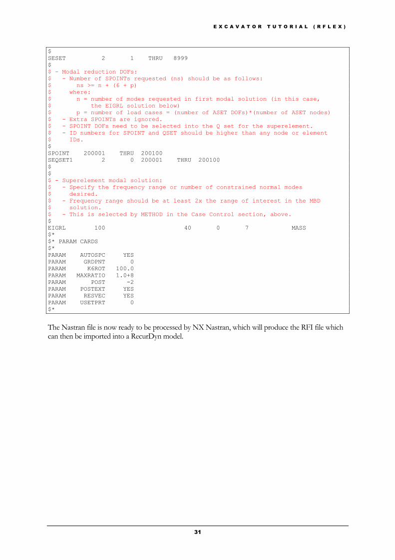
The Nastran file is now ready to be processed by NX Nastran, which will produce the RFI file which can then be imported into a RecurDyn model.


32

Appendix B : Supported FE

Elements

In this chapter, you can see the supported Fe elements in RecurDyn. To see more information, refer to RFlex of RecurDyn Help.

Appendix

B


33

Ansys Element Library

Type ANSYS elements

1D Element Link1, Link8, Link10, Link11,

Beam3, Beam4, Beam23, Beam24, Beam44, Beam54, Beam188

Pipe16, Pipe20, Pipe59

2D Element Plane2, Plane25, Plane42, Plane82, Plane83

Shell28, Shell41, Shell43, Shell63, Shell91, Shell93, Shell99, Shell181

3D Element Solid45, Solid46, Solid64, Solid65, Solid72, Solid73, Solid92, Solid95, Solid185, Solid186, Solid187

Rigid Element Combin14, Combin37, Combin39, Combin40

Mass Element Mass 21

MSC/NASTRAN Element Library

Type MSC/NASTRAN elements

1D Element CBAR, CBEAM, CBEND, CONROD, CROD, CTUBE

2D Element CTRIA3, CTRIA6, CQUAD4, CQUAD8, CSHEAR

3D Element CTETRA, CPENTA, CHEXA

Rigid Element RBAR, RBE2, RBE3, RROD, CBUSH, CBUSH1D, CELAS1, CELAS2

Mass Element CONM1, CONM2


34

I-DEAS Element Library

Type I-DEAS elements

1D Element Rod, Linear Beam, Tapered Beam, Curved Beam

2D Element Thin Shell Linear Triangle, Thin Shell Parabolic Triangle, Thin Shell Linear Quadrilateral, Thin Shell Parabolic Quadrilateral,

Plane Stress Linear Triangle, Plane Stress Parabolic Triangle, Plane Stress Linear Quadrilateral, Plane Stress Parabolic Quadrilateral,

Plane Strain Linear Triangle, Plane Strain Parabolic Triangle, Plane Strain Linear Quadrilateral, Plane Strain Parabolic Quadrilateral

3D Element Solid Linear Tetrahedron, Solid Parabolic Tetrahedron, Solid Linear Wedge, Solid Parabolic Wedge, Solid Linear Brick, Solid Parabolic Brick

Rigid Element Rigid, Rigid Bar, Node To Node Translational Spring, Node To Node Rotational Spring

Mass Element Lumped Mass

Documents

Excavator Tutorial (RFlex) - RecurDyn Technical Supportsupport.recurdyn.com/wp-content/uploads/2015/11/RFlexExcavator... · FunctionBay, Inc. hereby grants to the licensed user the