Embed Size (px)
Citation preview
Evolutionary Game Theory for linguists.A primer
Gerhard Jager
Stanford University and University of Potsdam
1 Introduction: The evolutionary interpretation of GameTheory
Evolutionary Game Theory (EGT) was developed by theoretical biologists, espe-cially John Maynard Smith (cf. Maynard Smith 1982) as a formalization of theneo-Darwinian concept of evolution via natural selection. It builds on the insightthat many interactions between living beings can be considered to be games inthe sense of Game Theory (GT) — every participant has something to win or tolose in the interaction, and the payoff of each participant can depend on the ac-tions of all other participants. In the context of evolutionary biology, the payoff isan increase in fitness, where fitness is basically the expected number of offspring.According to the neo-Darwinian view on evolution, the units of natural selectionare not primarily organisms but heritable traits of organisms. If the behavior oforganisms, i.e., interactors, in a game-like situation is genetically determined, thestrategies can be identified with gene configurations.
2 Stability and dynamics
2.1 Evolutionary stability
Evolution is frequently conceptualized as a gradual progress towards more com-plexity and improved adaption. Everybody has seen pictures displaying a linearascent leading from algae over plants, fishes, dinosaurs, horses, and apes to Ne-anderthals and finally humans. Evolutionary biologist do not tire to point outthat this picture is quite misleading. (See for instance the discussion in Gould2002.) Darwinian evolution means a trajectory towards increased adaption to theenvironment, proceeding in small steps. If a local maximum is reached, evolution
1

2 Stability and dynamics 2
is basically static. Change may occur if random variation (due to mutations)accumulate so that a population leaves its local optimum and ascents anotherlocal optimum. Also, the fitness landscape itself may change as well—if the en-vironment changes, the former optima my cease to be optimal. Most of the timebiological evolution is macroscopically static though. Explaining stability is thusas important a goal for evolutionary theory than explaining change.
In the EGT setting, we are dealing with large populations of potential play-ers. Each player is programmed for a certain strategy, and the members of thepopulation play against each other very often under total random pairings. Thepayoffs of each encounter are accumulated as fitness, and the average numberof offspring per individual is proportional to its accumulated fitness, while thebirth rate and death rate are constant. Parents pass on their strategy to theiroffspring basically unchanged. Replication is to be thought of as asexual, i.e.,each individual has exactly one parent. If a certain strategy yields on averagea payoff that is higher than the population average, its replication rate will behigher than average and its proportion within the overall population increases,while strategies with a less-than-average expected payoff decrease in frequency. Astrategy mix is stable under replication if the relative proportions of the differentstrategies within the population do not change under replication.
Occasionally replication is unfaithful though, and an offspring is programmedfor a different strategy than its parent. If the mutant has a higher expectedpayoff (in games against members of the incumbent population) than the averageof the incumbent population itself, the mutation will spread and possibly drivethe incumbent strategies to extinction. For this to happen, the initial number ofmutants may be arbitrarily small.1 Conversely, if the mutant does worse than theaverage incumbent, it will be wiped out and the incumbent strategy mix prevails.
A strategy mix is evolutionarily stable if it is resistant against the invasionof small proportions of mutant strategies. In other words, an evolutionarily stablestrategy mix has an invasion barrier. If the amount of mutant strategies is lowerthan this barrier, the incumbent strategy mix prevails, while invasions of highernumbers of mutants might still be successful.
In the metaphor used here, every player is programmed for a certain strat-egy, but a population can be mixed and comprise several strategies. Instead wemay assume that all individuals are identically programmed, but this programis non-deterministic and plays different strategies according to some probabilitydistribution (which corresponds to the relative frequencies of the pure strate-gies in the first conceptualization). Game theorists call such non-deterministicstrategies mixed strategies. For the purposes of the evolutionary dynamics ofpopulations, the two models are equivalent. It is standard in EGT to talk of anevolutionarily stable strategy, where a strategy can be mixed, instead of an
1In the standard model of EGT, populations are — simplifyingly — thought of as infiniteand continuous, so there are no minimal units.
2 Stability and dynamics 3
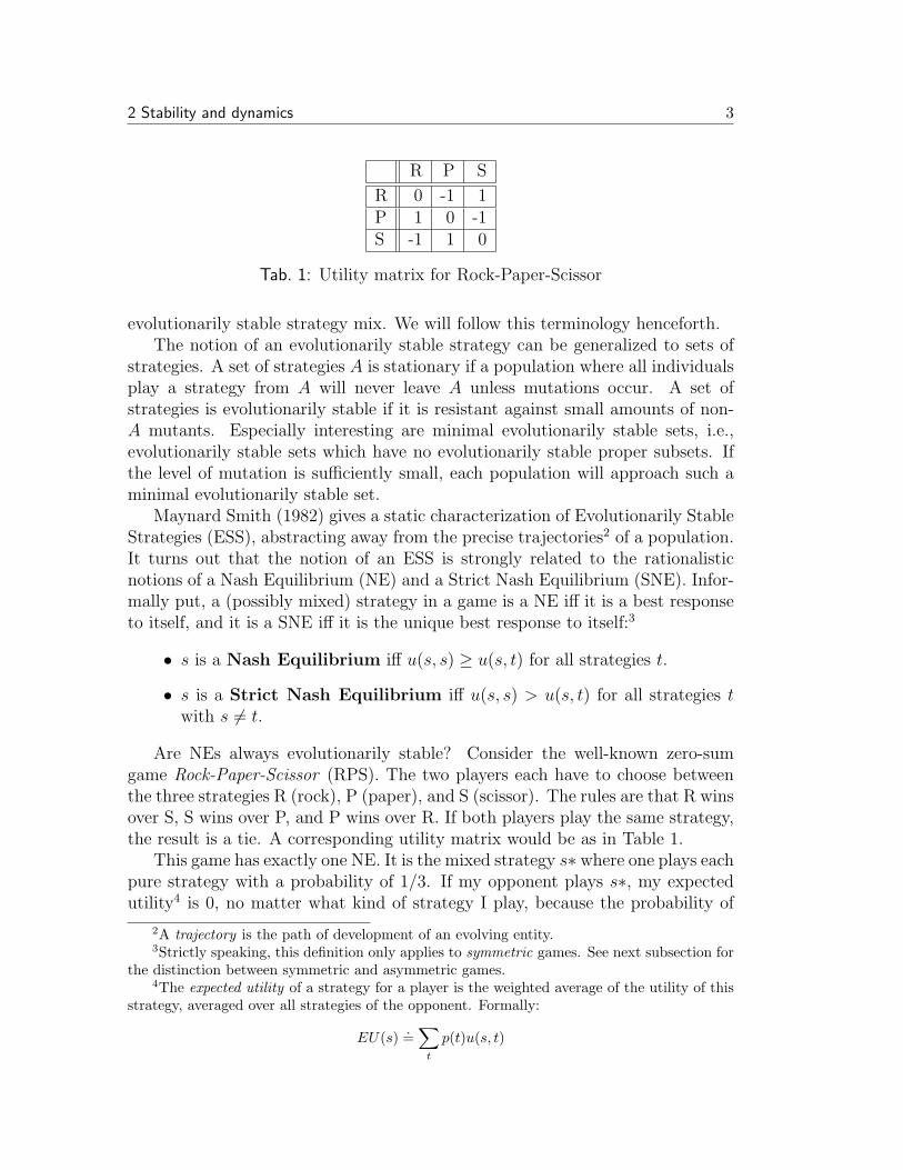
R P S
R 0 -1 1P 1 0 -1S -1 1 0
Tab. 1: Utility matrix for Rock-Paper-Scissor
evolutionarily stable strategy mix. We will follow this terminology henceforth.The notion of an evolutionarily stable strategy can be generalized to sets of
strategies. A set of strategies A is stationary if a population where all individualsplay a strategy from A will never leave A unless mutations occur. A set ofstrategies is evolutionarily stable if it is resistant against small amounts of non-A mutants. Especially interesting are minimal evolutionarily stable sets, i.e.,evolutionarily stable sets which have no evolutionarily stable proper subsets. Ifthe level of mutation is sufficiently small, each population will approach such aminimal evolutionarily stable set.
Maynard Smith (1982) gives a static characterization of Evolutionarily StableStrategies (ESS), abstracting away from the precise trajectories2 of a population.It turns out that the notion of an ESS is strongly related to the rationalisticnotions of a Nash Equilibrium (NE) and a Strict Nash Equilibrium (SNE). Infor-mally put, a (possibly mixed) strategy in a game is a NE iff it is a best responseto itself, and it is a SNE iff it is the unique best response to itself:3
• s is a Nash Equilibrium iff u(s, s) ≥ u(s, t) for all strategies t.
• s is a Strict Nash Equilibrium iff u(s, s) > u(s, t) for all strategies twith s 6= t.
Are NEs always evolutionarily stable? Consider the well-known zero-sumgame Rock-Paper-Scissor (RPS). The two players each have to choose betweenthe three strategies R (rock), P (paper), and S (scissor). The rules are that R winsover S, S wins over P, and P wins over R. If both players play the same strategy,the result is a tie. A corresponding utility matrix would be as in Table 1.
This game has exactly one NE. It is the mixed strategy s∗ where one plays eachpure strategy with a probability of 1/3. If my opponent plays s∗, my expectedutility4 is 0, no matter what kind of strategy I play, because the probability of
2A trajectory is the path of development of an evolving entity.3Strictly speaking, this definition only applies to symmetric games. See next subsection for
the distinction between symmetric and asymmetric games.4The expected utility of a strategy for a player is the weighted average of the utility of this
strategy, averaged over all strategies of the opponent. Formally:
EU(s) .=∑
t
p(t)u(s, t)
2 Stability and dynamics 4
winning, losing, or a tie are equal. So every strategy is a best response to s∗. Onthe other hand, if the probabilities of the strategies of my opponent are unequal,then my best response is always to play one of the pure strategies that win againstthe most probable of his actions. No strategy wins against itself; thus no otherstrategy can be a best response to itself. s∗ is the unique NE.
Is it evolutionarily stable? Suppose a population consists to equal parts of R,P, and S players, and they play against each other in random pairings. Then theplayers of each strategy have the same average utility, 0. If the number of offspringof each individual is positively correlated with its accumulated utility, there willbe equally many individuals of each strategy in the next generation again, andthe same in the second generation ad infinitum. s∗ is a steady state. However,Maynard Smith’s notion of evolutionary stability is stronger. An ESS should notonly be stationary, but it also be robust against mutations. Now suppose in apopulation as described above, some small proportion of the offspring of P-playersare mutants and become S-players. Then the proportion of P-players in the nextgeneration is slightly less than 1/3, and the share of S-players exceeds 1/3. Sowe have
p(S) > p(R) > p(P )
This means that R-players will have an average utility that is slightly higherthan 0 (because they win more against S and lose less against P). Likewise, S-players are at disadvantage because they win less than 1/3 of the time (againstP) but lose 1/3 of the time (against R). So one generation later, the configurationis
p(R) > p(P ) > p(S)
By an analogous argument, the next generation will have the configuration
p(P ) > p(S) > p(R)
etc. After the mutation, the population has entered a circular trajectory,without ever approaching the stationary state s∗ again without further mutations.
So not every NE is an ESS. The converse does hold though. Suppose a strategys were not a NE. Than there would be a strategy t with u(t, s) > u(s, s). Thismeans that a t-mutant in a homogeneous s-population would achieve a higheraverage utility than the incumbents and thus spread. This may lead to theeventual extinction of s, a mixed equilibrium or a circular trajectory, but thepure s-population is never restored. Hence s is not an ESS. By contrapositionwe conclude that each ESS is a NE.
Can we identify ESSs with SNEs? Not quite. Imagine a population of pigeonswhich come in two variants. A-pigeons have a perfect sense of orientation andcan always find their way. B-pigeons have no sense of orientation at all. Suppose

2 Stability and dynamics 5
A B
A 1 1B 1 0
Tab. 2: Utility matrix of the pigeon orientation game
that pigeons always fly in pairs. There is no big disadvantage of being a B ifyour partner is of type A because he can lead the way. Likewise, it is of nodisadvantage to have a B-partner if you are an A because you can lead the wayyourself. (Let us assume for simplicity that leading the way has neither costsno benefits.) However, a pair of B-individuals has a big disadvantage because itcannot find its way. Sometimes these pairs get lost and starve before they canreproduce. This corresponds to the utility matrix in Table 2.
A is a NE, but not an SNE, because u(B, A) = u(A, A). Now imagine thata homogeneous A-population is invaded by a small group of B-mutants. Ina predominantly A-population, these invaders fare as good as the incumbents.However, there is a certain probability that a mutant goes on a journey withanother B-mutant. Then both are in danger. Hence, sooner or later B-mutantswill approach extinction because they cannot interact very well with their peers.More formally, suppose the proportions of A and B in the populations are 1− εand ε respectively. Then the average utility of A is 1, while the average utilityof B is only 1 − ε. Hence the A-subpopulation will grow faster than the B-subpopulation, and the share of B-individuals converges towards 0.
Another way to look at this scenario is this: B-invaders cannot spread in a ho-mogeneous A-population, but A-invaders can successfully invade a B-populationbecause u(A, B) > u(B, B). Hence A is immune against B-mutants.
If a strategy is immune against any kind of mutants in this sense, it is evolu-tionarily stable. The necessary and sufficient condition for evolutionary stabilityare (according to Maynard Smith 1982):
• s is an Evolutionarily Stable Strategy iff
1. u(s, s) ≥ u(t, s) for all t, and
2. if u(s, s) = u(t, s) for some t 6= s, then u(s, t) > u(t, t).
The first clause requires an ESS to be a NE. The second clause says that if at-mutation can survive in an s-population, s must be able to successfully invadeany t-population for s to be evolutionarily stable.
From the definition it follows immediately that each SNE is an ESS. So wehave the inclusion relation
Strict Nash Equilibria ⊂ Evolutionarily Stable Strategies ⊂ Nash Equilibria
2 Stability and dynamics 6
2.2 The replicator dynamics
The considerations that lead to the notion of an ESS are fairly general. Theyrest on three crucial assumptions:
1. Populations are (practically) infinite.
2. Each pair of individuals is equally likely to interact.
3. The expected number of offspring of an individual (i.e., its fitness in theDarwinian sense) is monotonically related to its average utility.
The assumption of infinity is crucial for two reasons. First, individuals usually donot interact with themselves under most interpretations of EGT. Thus, in a finitepopulation, the probability to interact with a player using the same strategy asoneself would be less than the share of this strategy in the overall population.If the population is infinite, this discrepancy disappears. Second, in a finitepopulation the average utility of players of a given strategy converges towards itsexpected value, but it need not be identical to it. This introduces a stochasticcomponent. While this kind of stochastic EGT is a lively sub-branch of EGT (seebelow), the standard interpretation of EGT assumes deterministic evolution. Inan infinite population, the average utility coincides with the expected utility.
As mentioned before, the evolutionary interpretation of GT interprets utilitiesas fitness. The notion of an ESS makes the weaker assumption that there is justa positive correlation between utility and fitness—a higher utility translates intomore expected offspring, but this relation need not be linear. This is importantfor applications of EGT to cultural evolution, where replication proceeds vialearning and imitation, and utilities correspond to social impact. There might beindependent measures for utility that influence fitness without being identical toit.
Nevertheless it is often helpful to look at a particular population dynamicsto sharpen one’s intuition about the evolutionary behavior of a game. Also, ingames as Rock-Paper-Scissor, a lot of interesting things can be said about theirevolution even though they have no stable states at all. Therefore we will discussone particular evolutionary game dynamics in some detail.
The easiest way to relate utility and fitness in a monotonic way is of coursejust to identify them. So let us assume that the average utility of an individualequals its expected number of offspring.
The remainder of this section requires some elementary calculus. Readers whodo not have this kind of mathematical background can go directly to the nextsection without too much loss of continuity.
To keep the math manageable, we assume that the population size is a realvalued function N(t) of the time t. It can be thought of as the actual (discrete)population size divided by some normalization constant for the borderline casewhere both approach infinity. In a first step, we assume the time t to be discrete.

2 Stability and dynamics 7
In each time step, each individual spawns offspring according to its average utility.Furthermore, a certain constant proportion d of the population dies, and theprobability to die is independent from the strategy of the victim. Let us say thatthere are n strategies s1, . . . , sn. The amount of individuals playing strategy i iswritten as Ni. The relative frequency of strategy si, i.e., Ni/N , is written as xi
for short. (Note that x is a probability distribtion, i.e.∑
j xj = 1.)The discrete time dynamics is
Ni(t + 1) = Ni(t) + Ni(t)(n∑
j=1
xju(i, j)− d) (1)
Now let us extrapolate this to a continuous time variable. Suppose individualsare born and die continuously. We can generalize to arbitrary time intervals ∆t:
Ni(t + ∆t) = Ni + ∆tNi(n∑
j=1
xju(i, j)− d) (2)
and from this we derive directly
∆Ni
∆t= Ni(
n∑j=1
xju(i, j)− d) (3)
When ∆t goes towards 0, we get converge towards the limiting
dNi
dt= Ni(
n∑j=1
xju(i, j)− d) (4)
The size of the population as a whole may also change, depending on thepopulation average of the population.
N(t + ∆t) =n∑
i=1
(Ni + ∆t(Ni
n∑j=1
xju(i, j)− d)) (5)
= N + ∆t(Nn∑
i=1
xi
n∑j=1
xju(i, j)− d) (6)
By a similar derivation as above, we get the differential equation
dN
dt= N(
n∑i=1
xi
n∑j=1
xju(i, j)− d) (7)
2 Stability and dynamics 8
We abbreviate the expected utility of strategy si,∑n
j=1 xju(i, j), as ui, and thepopulation average of the expected utility,
∑ni=1 xiui, as u. So the two differential
equations can be written as
dNi
dt= Ni(ui − d) (8)
dN
dt= N(u− d) (9)
We are not really interested in the dynamics of the absolute size of the popu-lation and its subpopulations, but in the dynamics of xi, the share of the differentstrategies within the global population. By definition, xi = Ni/N , and by thedivision rule for the first derivative, we have
dxi
dt=
(NNi(ui − d)− (NiN(ui − d)))
N2(10)
= xi(ui − u) (11)
The latter differential equation is called the replicator dynamics. It was firstintroduced in Taylor and Jonker (1978). It is worth a closer examination. It saysthat the reproductive success of strategy si depends on two factors. First, thereis the abundance of si itself, xi. The more individuals in the current populationare of type si, the more likely it is that there will be offspring of this type. Theinteresting part is the second factor, the differential utility. If ui = u, this meansthat strategy si does exactly as good as the population average. In this case thetwo terms cancel each other out, and dxi
dt= 0. This means that si’s share of the
total population remains constant. If ui > u, si does better than average, and itincreases its share. Likewise, a strategy si with a less-than-average performance,i.e., ui < u, loses ground.
Intuitively, evolutionary stability means a state is (a) stationary and (b) im-mune against the invasion of small numbers of mutations. This can directly betranslated into dynamic notions. To require that a state is stationary amountsto saying that the relative frequencies of the different strategies within the pop-ulation do not change over time. In other words, the vector x is stationary iff forall i:
dxi
dt= 0
This is the case if either xi = 0 or ui = u for all i.Robustness against small amounts of mutation means that there is an envi-
ronment of x such that all trajectories leading through this environment actuallyconverge towards x. In the jargon of dynamic systems, x is then asymptoticallystable or a point attractor. It can be shown that a (possibly mixed) strategy isan ESS if and only if it is asymptotically stable under the replicator dynamics.
2 Stability and dynamics 9
0
0.2
0.4
0.6
0.8
1
t
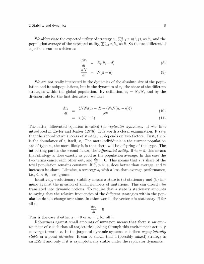
Fig. 1: Replicator dynamics of the pigeon orientation game
The replicator dynamics enables us to display the evolutionary behavior of agame graphically. This has a considerable heuristic value. There are basicallytwo techniques for this. First, it is possible to depict time series in a Cartesiancoordinate system. The time is mapped to the x-axis, while the y-axis corre-sponds to the relative frequency of some strategy. For some sample of initialconditions, the development of the relative frequencies over time is plotted as afunction of the time variable. In a two-strategy game like the pigeon orientationscenario discussed above, this is sufficient to exhaustively display the dynamicsof the system because the relative frequencies of the two strategies always sumup to 1. Figure 1 gives a few sample time series for the pigeon game. Here they-axis corresponds to the relative frequency of the A-population. It is plainlyobvious that the state where 100% of the population are of type A is in fact anattractor.
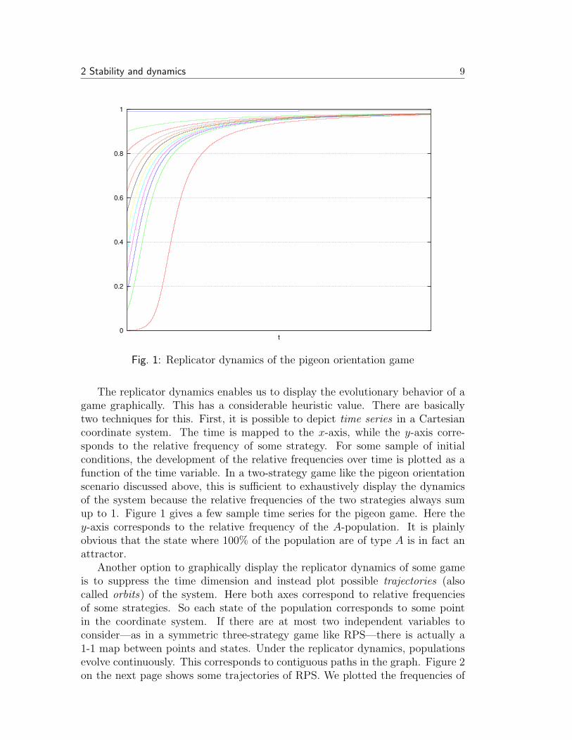
Another option to graphically display the replicator dynamics of some gameis to suppress the time dimension and instead plot possible trajectories (alsocalled orbits) of the system. Here both axes correspond to relative frequenciesof some strategies. So each state of the population corresponds to some pointin the coordinate system. If there are at most two independent variables toconsider—as in a symmetric three-strategy game like RPS—there is actually a1-1 map between points and states. Under the replicator dynamics, populationsevolve continuously. This corresponds to contiguous paths in the graph. Figure 2on the next page shows some trajectories of RPS. We plotted the frequencies of

2 Stability and dynamics 10
R
S
Fig. 2: Replicator dynamics of the rock-paper-scissor game
the “rock” strategy and the “scissor” strategy against the y-axis and the x-axisrespectively. The sum of their frequencies never exceeds 1. This is why the wholeaction happens in the lower left corner of the square. The relative frequencyof “paper” is uniquely determined by the two other strategies and is thus noindependent variable.
The circular nature of this dynamics that we informally uncovered above isclearly to discern. One can also easily see “with the bare eye” that this game hasno attractor, i.e., no ESS.
There are plenty of different softwares on the market to produce such plots.We used the freely available program “Gnuplot” (combined with some numericalscript language like “Octave” or “Python” to do the actual numerical computa-tions) for the graphics shown here. There are also various commercial programslike “Mathematica” or “Matlab” which have more options (and are better docu-mented!).
2.3 Asymmetric games
So far we considered symmetric games. Formally, a game is symmetric if thetwo players have the same set of strategies to choose from, and the utility does
2 Stability and dynamics 11
H D
H 1 7D 2 3
Tab. 3: Hawks and Doves
not depend on the position of the players. If u1 is the utility matrix for the rowplayer, and u2 of the column player, then the game is symmetric iff both matricesare square (have the same number of rows and columns), and
u1(i, j) = u2(j, i)
There are various scenarios where these assumptions are inappropriate. Inmany types of interaction, the participants assume certain roles. In contests overa territory, it makes a difference who is the incumbent and who the intruder. Ineconomic interaction, buyer and seller have different options at their disposal.Likewise in linguistic interaction you are the speaker or the hearer. The lastexample illustrates that it is possible for the same individual to assume eitherrole at different occasions. If this is not possible, we are effectively dealing withtwo disjoint populations, like predators and prey or females and males in biology,haves and have-nots in economics, and adults and infants in language acquisition(in the latter case infants later become adults, but these stages can be considereddifferent games).
The dynamic behavior of asymmetric games differs markedly from symmetricones. The ultimate reason for this is that in a symmetric game, an individual canquasi play against itself (or against a clone of himself), while this is impossiblein asymmetric games. The well-studied game “Hawks and Doves” may serve toillustrate this point. Imagine a population where the members have frequentdisputes over some essential resource (foot, territory, mates, whatever). Thereare two strategies to deal with a conflict. The aggressive type (the “hawks”) willnever give in. If two hawks come in conflict, they fight it out until one of themdies. The other one gets the resource. The doves, on the contrary, embark upona lengthy ritualized dispute until one of them is tired of it and gives in. If a hawkand a dove meet, the dove gives in right away and the hawk gets the resourcewithout any effort. There are no other strategies.
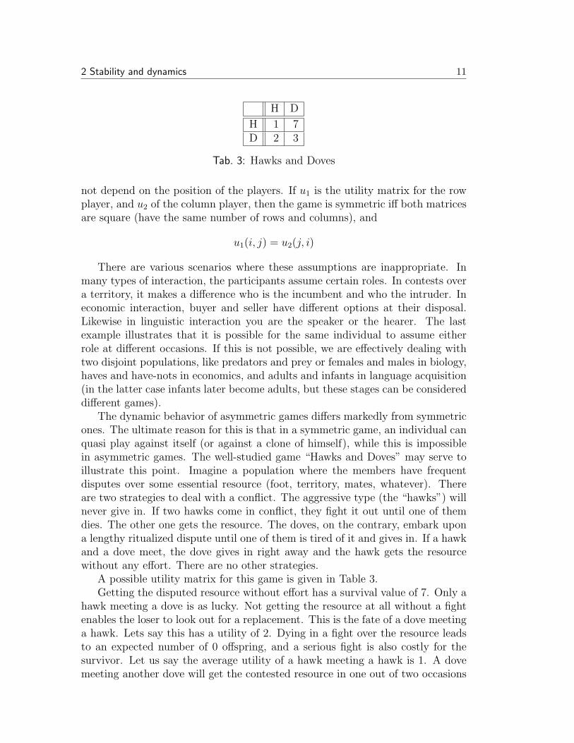
A possible utility matrix for this game is given in Table 3.Getting the disputed resource without effort has a survival value of 7. Only a
hawk meeting a dove is as lucky. Not getting the resource at all without a fightenables the loser to look out for a replacement. This is the fate of a dove meetinga hawk. Lets say this has a utility of 2. Dying in a fight over the resource leadsto an expected number of 0 offspring, and a serious fight is also costly for thesurvivor. Let us say the average utility of a hawk meeting a hawk is 1. A dovemeeting another dove will get the contested resource in one out of two occasions
2 Stability and dynamics 12
0
0.2
0.4
0.6
0.8
1
t
Fig. 3: Symmetric Hawk-and-Dove game
on average, but the lengthy ritualistic contest comes with a modest cost too, sothe utility of a dove meeting a dove could be 3.
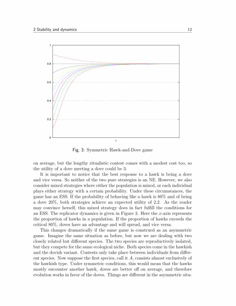
It is important to notice that the best response to a hawk is being a doveand vice versa. So neither of the two pure strategies is an NE. However, we alsoconsider mixed strategies where either the population is mixed, or each individualplays either strategy with a certain probability. Under these circumstances, thegame has an ESS. If the probability of behaving like a hawk is 80% and of beinga dove 20%, both strategies achieve an expected utility of 2.2. As the readermay convince herself, this mixed strategy does in fact fulfill the conditions foran ESS. The replicator dynamics is given in Figure 3. Here the x-axis representsthe proportion of hawks in a population. If the proportion of hawks exceeds thecritical 80%, doves have an advantage and will spread, and vice versa.
This changes dramatically if the same game is construed as an asymmetricgame. Imagine the same situation as before, but now we are dealing with twoclosely related but different species. The two species are reproductively isolated,but they compete for the same ecological niche. Both species come in the hawkishand the dovish variant. Contests only take place between individuals from differ-ent species. Now suppose the first species, call it A, consists almost exclusively ofthe hawkish type. Under symmetric conditions, this would mean that the hawksmostly encounter another hawk, doves are better off on average, and thereforeevolution works in favor of the doves. Things are different in the asymmetric situ-
2 Stability and dynamics 13
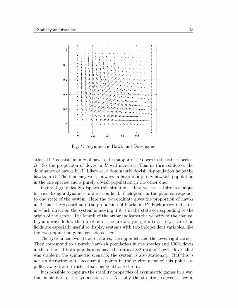
Fig. 4: Asymmetric Hawk-and-Dove game
ation. If A consists mainly of hawks, this supports the doves in the other species,B. So the proportion of doves in B will increase. This in turn reinforces thedominance of hawks in A. Likewise, a dominantly dovish A-population helps thehawks in B. The tendency works always in favor of a purely hawkish populationin the one species and a purely dovish population in the other one.
Figure 4 graphically displays this situation. Here we use a third techniquefor visualizing a dynamics, a direction field. Each point in the plain correspondsto one state of the system. Here the x-coordinate gives the proportion of hawksin A, and the y-coordinate the proportion of hawks in B. Each arrow indicatesin which direction the system is moving if it is in the state corresponding to theorigin of the arrow. The length of the arrow indicates the velocity of the change.If you always follow the direction of the arrows, you get a trajectory. Directionfields are especially useful to display systems with two independent variables, likethe two-population game considered here.
The system has two attractor states, the upper left and the lower right corner.They correspond to a purely hawkish population in one species and 100% dovesin the other. If both populations have the critical 8:2 ratio of hawks:doves thatwas stable in the symmetric scenario, the system is also stationary. But this isnot an attractor state because all points in the environment of this point arepulled away from it rather than being attracted to it.
It is possible to capture the stability properties of asymmetric games in a waythat is similar to the symmetric case. Actually the situation is even easier in
2 Stability and dynamics 14
the asymmetric case. The definition of a symmetric ESS was complicated by theconsideration that mutants may encounter other mutants. In a two-populationgame, this is impossible. In a one-population role game, this might happen.However, minimal mutations only affect strategies in one of the two roles. Ifsomebody minimally changes his grammatical preferences as a speaker, say, hisinterpretive preferences need not be affected by this.5 So while a mutant mightinteract with its clone, it will never occur that a mutant strategy interacts withitself, because, by definition, the two strategy sets are distinct. So, the secondclause of the definition of ESS doesn’t matter.
We have to make some conceptual adjustments for the asymmetric case. Sincethe two strategy sets are distinct, the utility matrices are distinct as well. Ina game between m and n strategies, the utility function of the first player isdefined by an m × n matrix, call it uA, and an n ×m matrix uB for the secondplayer. An asymmetric Nash Equilibrium is now a pair of strategies, one foreach population/role, such that each component is the best response to the othercomponent. Likewise, a SNE is a pair of strategies where each one is the uniquebest response to the other.
Now if the second clause in the definition of a symmetric ESS plays no rolehere, does this mean that only the first clause matters? In other words, are all andonly the NEs evolutionarily stable in the asymmetric case? Not quite. Supposea situation as before, but now species A consists of three variants instead of two.The first two are both aggressive, and they both get the same, hawkish utility.Also, individuals from B get the same utility from interacting with either of thetwo types of hawks in A. The third A-strategy are still the doves. Now supposethat A consists exclusively of hawks of the first type, and B only of doves. Thenthe system is in an NE, since both hawk strategies are the best response to thedoves in B, and for a B-player, being a dove is the best response to either hawk-strategy. If this A-population is invaded by a mutant of the second hawkish type,the mutants are exactly as fit as the incumbents. They will neither spread nor beextinguished. (Biologists call this phenomenon drift—change that has no impactfor survival fitness and is driven by pure chance.) In this scenario, the system isin a (non-strict) NE, but it is not evolutionarily stable.
A strict NE is always evolutionarily stable though, and it can be shown(Selten 1980) that :
In asymmetric games, a configuration is an ESS iff it is a SNE.
It is a noteworthy fact about asymmetric games that ESSs are always purein the sense that both populations play one particular strategy with 100% prob-ability. This does not imply though that asymmetric games always settle in a
5One might argue that the strategies of a language user in these two roles are not indepen-dent. If this correlation is deemed to be important, the whole scenario has to be formalized asa symmetric game. See below for techniques of how to symmetrize asymmetric games.

2 Stability and dynamics 15
pure state. Not every asymmetric game has an ESS. The asymmetric version ofrock-paper-scissor, for instance, shows the same kind of cyclic dynamics as thesymmetric variant.
As in the symmetric case, this characterization of evolutionary stability iscompletely general and holds for all utility monotonic dynamics. Again, the sim-plest instance of such a dynamic is the replicator dynamic. Here a state is char-acterized by two probability vectors, x and y. They represent the probabilities ofthe different strategies in the two populations or roles. By similar considerationsas above, the dynamics of the asymmetric replicator dynamics can be describedby the system of differential equations:
dxi
dt= xi(
n∑j=1
yjuA(i, j)−m∑
k=1
xk
n∑j=1
yjuA(k, j)) (12)
dyi
dt= yi(
m∑j=1
xjuB(i, j)−n∑
k=1
yk
m∑j=1
xjuB(k, j)) (13)
It is straightforward to transform an asymmetric game into a symmetric game.In the previous setup, we had a population A with m strategies and a utilitymatrix ua, interacting with a population B with n strategies and a utility matrixuB. We may construct the set of pairs from A and B respectively and considereach such pair as a member of an abstract meta-population, being engaged in ameta-game. Every pair of interactions in the original game corresponds to oneinteraction in the meta-game. If a1 interacted with b1 and a2 with b2 in theoriginal game, this amounts to an interaction of 〈a1, b2〉 with 〈a2, b1〉 in the newgame. If SA and SB are the strategy sets in the original game, the meta-gamehas just one such set, SA ∪ SB. Since SA and SB are disjoint by definition, thereare m + n meta-strategies.
The utility of a combined strategy is the sum of the utilities of the componentstrategies. If we call the meta-utility function uAB, we have
uAB(〈i, j〉, 〈k, l〉) = uA(i, l) + uB(j, k)
The meta-game is a symmetric game. It turns out that the replicator dynam-ics of the meta-population can be described by the standard symmetric replicatordynamics. Also every SNE, this is, every ESS, in the original game correspondsto an ESS in the meta-game.
So the essential dynamic characteristics of an asymmetric game are thus pre-served when it is symmetrized. On the other hand, reducing a symmetric gameto an asymmetric one is not possible. This is probably the reason why asymmet-ric games are usually not given much attention in the literature. For practicalpurposes, it does make quite a difference though whether you have to deal witha 3 × 10 asymmetric game, say, or with the 30 × 30 symmetrized version of it.Especially applications of GT in linguistic pragmatics frequently deal with the
3 EGT and language 16
asymmetry between speaker and hearer. A formalization as asymmetric gamemight thus be more natural here. Also, in more sophisticated dynamic modelslike spatial EGT, an asymmetric game need not be reducible to a symmetric one.
3 EGT and language
Natural language is an interactive and self-replicative system. This makes EGTa promising analytical tool for the study of linguistic phenomena. Let us startthis section with a few general remarks.
To give an EGT formalization—or an evolutionary conceptualization in gene-ral—of a particular empirical phenomenon, various issues have to be addressedin advance. What is replication in the domain in question? What are the repli-cators? Is replication faithful, and if so, which features are constant under repli-cation? What factors influence reproductive success (= fitness)? What kind ofvariation exists, and how does it interact with replication?
There are various aspects of natural language that are subject to replication,variation and selection, on various timescales that range from minutes (singlediscourse) till millennia (language related aspects of biological evolution). Wewill focus on cultural (as opposed to biological) evolution on short time scales,but we will briefly discuss the more general picture.
The most obvious mode of linguistic self-replication is first language acqui-sition. Before this can take effect, the biological preconditions for language ac-quisition and use have to be given, ranging from the physiology of the ear andthe vocal tract to the necessary cognitive abilities. The biological language fac-ulty is replicated in biological reproduction. It seems obvious that the ability tocommunicate does increase survival chances and social standing and thus pro-motes biological fitness, but only at a first glance. Sharing information usuallybenefits the receiver more than the sender. Standard EGT predicts this kind ofaltruistic behavior to be evolutionarily unstable. Here is a crude formalizationin terms of an asymmetric game between sender and receiver. The sender has achoice between sharing information (“T” for “talkative”) or keeping informationfor himself (“S” for “silent”). The (potential) receiver has the options of payingattention and trying to decode the messages of the sender (“A” for “attention”)or to ignore (“I”) the sender. Let us say that sharing information does have acertain benefit for the sender because it may serve to manipulate the receiver.On the other hand, sending a signal comes with an effort and may draw the at-tention of predators. For the sake of the argument, we assume that the costs andbenefits are roughly equally distributed given the receiver pays attention. If thereceiver ignores the message, it is disadvantageous for the sender to be talkative.For the receiver, it pays to pay attention if the sender actually sends. Then thelistener benefits most. If the sender is silent, it is of disadvantage for the listenerto pay attention because attention is a precious resource that could have been
3 EGT and language 17
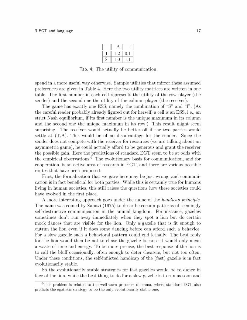
A I
T 1,2 0,1S 1,0 1,1
Tab. 4: The utility of communication
spend in a more useful way otherwise. Sample utilities that mirror these assumedpreferences are given in Table 4. Here the two utility matrices are written in onetable. The first number in each cell represents the utility of the row player (thesender) and the second one the utility of the column player (the receiver).
The game has exactly one ESS, namely the combination of “S” and “I”. (Asthe careful reader probably already figured out for herself, a cell is an ESS, i.e., anstrict Nash equilibrium, if its first number is the unique maximum in its columnand the second one the unique maximum in its row.) This result might seemsurprising. The receiver would actually be better off if the two parties wouldsettle at (T,A). This would be of no disadvantage for the sender. Since thesender does not compete with the receiver for resources (we are talking about anasymmetric game), he could actually afford to be generous and grant the receiverthe possible gain. Here the predictions of standard EGT seem to be at odds withthe empirical observations.6 The evolutionary basis for communication, and forcooperation, is an active area of research in EGT, and there are various possibleroutes that have been proposed.
First, the formalization that we gave here may be just wrong, and communi-cation is in fact beneficial for both parties. While this is certainly true for humansliving in human societies, this still raises the questions how these societies couldhave evolved in the first place.
A more interesting approach goes under the name of the handicap principle.The name was coined by Zahavi (1975) to describe certain patterns of seeminglyself-destructive communication in the animal kingdom. For instance, gazellessometimes don’t run away immediately when they spot a lion but do certainmock dances that are visible for the lion. Only a gazelle that is fit enough tooutrun the lion even if it does some dancing before can afford such a behavior.For a slow gazelle such a behavioral pattern could end lethally. The best replyfor the lion would then be not to chase the gazelle because it would only meana waste of time and energy. To be more precise, the best response of the lion isto call the bluff occasionally, often enough to deter cheaters, but not too often.Under these conditions, the self-inflicted handicap of the (fast) gazelle is in factevolutionarily stable.
So the evolutionarily stable strategies for fast gazelles would be to dance inface of the lion, while the best thing to do for a slow gazelle is to run as soon and
6This problem is related to the well-worn prisoners dilemma, where standard EGT alsopredicts the egotistic strategy to be the only evolutionarily stable one.
3 EGT and language 18
as fast as possible. Given this, the dance is a form of communication betweenthe gazelle and the lion, expressing “I am faster than you”.
The crucial insight here is that truthful communication can be evolutionarilystable if lying is more costly than communicating the truth. A slow gazelle couldtry to use the mock dance as well to discourage a lion from hunting it, butthis would be risky if the lion occasionally calls the bluff. The expected costsof such a strategy are thus higher than the costs of running away immediately.In communication among humans, there are various way how lying might bemore costly than telling (or communicating) the truth. To take an example fromeconomics, driving a Rolls Royce communicates “I am rich” because for a poorman, the costs of buying and maintaining such an expensive car outweigh itsbenefits while a rich man can afford them. Here producing the signal as suchis costly. In linguistic communication, lying comes with the social risk of beingfound out, so in many cases telling the truth is more beneficial than lying.
The idea of the handicap principle as evolutionary basis for communicationhas inspired a plethora of research in biology and economics. Van Rooij (2003)uses it to give a game theoretic explanation of politeness as a pragmatic phe-nomenon.
A third hypothesis rejects the assumption of standard EGT that all indi-viduals interact with equal probability. When I increase the fitness of my kin,I thereby increase the chances for replication of my own gene pool, even if itshould be to my own disadvantage. Recall that utility in EGT does not meanthe reproductive success of an individual but of a strategy, and strategies cor-respond to heritable traits in biology. A heritable trait for altruism might thushave a high expected utility provided its carriers preferably interacts with othercarriers of this trait. Biologists call this model kin selection. There are variousmodifications of EGT that give up the assumption of random pairing. We willreturn to this issue later on.
Natural languages are not passed on via biological but via cultural transmis-sion. First language acquisition is thus a qualitatively different mode of repli-cation. Most applications of evolutionary thinking in linguistics focus on theensuing acquisition driven dynamics. It is an important aspect in understandinglanguage change on a historical timescale of decades and centuries.
It is important to notice that there is a qualitative difference between Dar-winian evolution and the dynamics that results from iterated learning (in thesense of iterated first language acquisition). In Darwinian evolution, replicationis almost always faithful. Variation is the result of occasional unfaithful replica-tion, a rare and essentially random event. Theories that attempt to understandlanguage change via iterated language acquisition stress the fact though that here,replication can be unfaithful in a systematic way. The work of Martin Nowakand his co-workers (see for instance Nowak et al. 2002) is a good representativeof this approach. They assume that an infant that grows up in a community ofspeaker of some language L1 might acquire another language L2 with a certain
3 EGT and language 19
probability. This means that those languages will spread in a population that(a) are likely targets of acquisition for children that are exposed to other lan-guages, and (b) are likely to be acquired faithfully themselves. This approachthus conceptualizes language change as a Markov process7 rather than evolutionthrough natural selection. Markov processes and natural selection of course donot exclude each other. Nowak’s differential equation describing the languageacquisition dynamics actually consist of a basically game theoretical natural se-lection component (pertaining to the functionality of language) and a (learningoriented) Markov component.
Language gets replicated on a much shorter time scale, just via being used.The difference between acquisition based and usage based replication can be il-lustrated by looking at the development of the vocabulary of some language.There are various ways how a new word can enter a language—morphologicalcompounding, borrowing from other languages, lexicalization of names, coinageof acronyms, what have you. Once a word is part of a language, it is gradu-ally adapted to this language, i.e., it acquires a regular morphological paradigm,its pronunciation is nativized etc. The process of establishing a new word ispredominantly driven by mature (adult or adolescent) language users, not by in-fants. Somebody introduces the new word, and people start imitating it. Whetherthe new coinage catches on depends on whether there is a need for this word,whether it fills a social function (like distinguishing the own social group fromother groups), on the social prestige of the persons who already use it etc.
Since the work of Labov (see for instance Labov 1972) functionally orientedlinguists have repeatedly pointed out that grammatical change actually follows asimilar pattern. The main agents of language change, they argue, are mature lan-guage users rather than children.8 Not just the vocabulary is plastic and changesvia language use but all kinds of linguistic variables like syntactic constructions,phones, morphological devices, interpretational preferences etc. Imitation playsa crucial part here, and imitation is of course a kind of replication. Unlike inbiological replication, the usage of a certain word or construction can usuallynot be traced back to a unique model or pair of models that spawn the tokenin question. Rather, every previous usage of this linguistic item that the usertook notice of shares a certain fraction of “parenthood”. Recall though that thebasic units of evolution in EGT are not individuals but strategies, and evolutionis about the relative frequency of strategies. If there is a causal relation betweenthe abundance of a certain linguistic variant at a given point in time and its abun-
7A Markov process is a stochastic process where the system is always in one of finitely manystates, and where the probability of the possible future behaviours of the system only dependson its current state, not on its history.
8If true, this of course entails that the linguistic competence of adult speaker remainsplastic. While this seems to be at odds with some versions of generative grammar, the workof Tony Kroch (see for instance Kroch 2000) shows that this is perfectly compatible with aprinciples-and-parameters conception of grammar.

4 Pragmatics and EGT 20
dance at a later point, we can consider this a kind of faithful replication. Also,replication is almost but not absolutely faithful. This leads to a certain degreeof variation. Competing variants of a linguistic item differ in their likelihood tobe imitated—this corresponds to fitness and thus to natural selection. The usagebased dynamics of language use has all aspects that are required for a modelingin terms of EGT.
In the linguistic examples that we will discuss further on, we will assume thelatter notion of linguistic evolution.
4 Pragmatics and EGT
In this section we will go through a couple of examples that demonstrate how EGTcan be used to explain high level linguistic notions like pragmatic preferences orfunctional pressure.
4.1 Partial blocking
If there are two comparable expressions in a language such that the first is strictlymore specific than the second, there is a tendency to reserve the more generalexpression for situations where the more specific one is not applicable. A stan-dard example is the opposition between “many” and “all”. If I say that manystudents came to the guest lecture, it is usually understood that not all stu-dents came. There is a straightforward rationalistic explanation for this in termsof conversational maxims: the speaker should be as specific as possible. If thespeaker uses “many”, the hearer can conclude that the usage of “all” would havebeen inappropriate. This conclusion is strictly speaking not valid though—it isalso possible that the speaker just does not know whether all students came orwhether a few were missing.
A similar pattern can be found in conventionalized form in the organizationof the lexicon. If a regular morphological derivation and a simplex word compete,the complex word is usually reserved for cases where the simplex is not applicable.For instance, the compositional meaning of the English noun “cutter” is justsomeone or something that cuts. A knife is an instrument for cutting, but stillyou cannot call a knife a “cutter”. The latter word is reserved for non-prototypicalcutting instruments.
Let us consider the latter example more closely. We assume that the literalmeaning of “cutter” is a concept cutter’ and the literal meaning of “knife” aconcept knife’ such that every knife is a cutter but not vice versa, i.e.,
knife’ ⊂ cutter’
There are two basic strategies to use these two words, the semantic (S) andthe pragmatic (P ) strategy. Both come in two versions, a hearer strategy and

4 Pragmatics and EGT 21
a speaker strategy. A speaker using S will use “cutter” to refer to unspecifiedcutting instruments, and “knife” to refer to knifes. To refer to a cutting instru-ment that is not a knife, this strategy either uses the explicit “cutter but nota knife”, or, short but imprecise, also “cutter”. A hearer using S will interpretevery expression literally, i.e., “knife” means knife’, “cutter” means cutter’,and “cutter but not a knife” means cutter’− knife’.
A speaker using P will reserve the word “cutter” for the concept cutter’−knife’. To express the general concept cutter’, this strategy has to take resortto a more complex expression like “cutter or knife”. Conversely, a hearer usingP will interpret “cutter” as cutter’ − knife’, “knife” as knife’, and “cutteror knife” as cutter’.
So we are dealing with an asymmetric 2× 2 game. What is the utility func-tion? In EGT, utilities are interpreted as the expected number of offspring. Inour linguistic interpretation this means that utilities express the likelihood of astrategy to be imitated. It is a difficult question to tease apart the factors thatdetermine the utility of a linguistic item in this sense, and ultimately it has to beanswered by psycholinguistic and sociolinguistic research. Since we have not un-dertaken this research so far, we will make up a utility function, using plausibilityarguments.
We start with the hearer perspective. The main objective of the hearer incommunication, let us assume, is to gain as much truthful information as pos-sible. The utility of a proposition for the hearer is thus inversely proportionalto its probability, provided the proposition is true. For the sake of simplicity,we only consider contexts where the nouns in question occur in upward entail-ing context. Therefore cutter’ has a lower information value than knife’ orcutter’−knife’. It seems also fair to assume that non-prototypical cutters arerarer talked about than knifes; thus the information value of knife’ is lower thanthe one of cutter’−knife’.
For concreteness, we make up some numbers. If i is the function that assignsa concept its information value, let us say that
i(knife’) = 30
i(cutter’− knife’) = 40
i(cutter’) = 20
The speaker wants to communicate information. Assuming only honest in-tentions, the information value that the hearer gains should also be part of thespeaker’s utility function. Furthermore, the speaker wants to minimize his effortthough. So as a second component of the speaker’s utility function, we assumesome complexity measure over expressions. A morphologically complex word like“cutter” is arguably more complex than a simple one like “knife”, and syntac-tically complex phrases like “cutter or knife” or “cutter but not knife” are even
4 Pragmatics and EGT 22
S P
S 23.86, 28.60 24.26, 29.00P 23.40, 29.00 25.40, 31.00
Tab. 5: knife vs. cutter
more complex. The following stipulated values for the cost function take theseconsiderations into account:
cost(“knife”) = 1
cost(“cutter”) = 2
cost(“cutter or knife”) = 40
cost(“cutter but not knife”) = 45
These costs and benefits are to be weighted—everything depends on how ofteneach of the candidate concepts is actually used. The most prototypical concept ofthe three is certainly knife’, while the unspecific cutter’ is arguably rare. Letus say that, conditioned to all utterance situations in question, the probabilitiesthat a speaker tries to communicate the respective concepts are
p(knife’) = .7
p(cutter’− knife’) = .2
p(cutter’) = .1
The utility of the speaker is then the difference between the average infor-mation value that he manages to communicate and the average costs that hehas to afford. The utility of the hearer is just the average value of the correctinformation that is received. The precise values of these utilities finally dependon how often a speaker of the S-strategy actually uses the complex “cutter butnot knife”, and how often he uses the shorter “cutter”. Let us assume for thesake of concreteness that he uses the short form in 60% of all times.
After some elementary calculations, this leads us to the following utility ma-trix. The speaker is assumed to be the row player and the hearer the columnplayer. As always, the first entry in each cell gives the utility of the row player,i.e., the speaker.
Both players receive the absolutely highest utility if both play P . This meansperfect communication with minimal effort. All other combinations involve somekind of communication failure because the hearer either interprets the speaker’suse of “cutter” either too strong or too weak occasionally.
4 Pragmatics and EGT 23
Fig. 5: Partial blocking: replicator dynamics
If both players start out with the semantic strategy, mutant hearers that usethe pragmatic strategy will spread because they get the more specific interpre-tation cutter’−knife’ right in all cases where the speaker prefers minimizingeffort over being explicit. The mutants will get all cases wrong where the speakermeant cutter’ by using “cutter”, but the advantage is greater. If the hearersemploy the pragmatic strategy, speakers using their pragmatic strategy will startto spread now because they will have a higher chance to get their message across.The combination P/P is the only strict Nash equilibrium in the game and thusthe only ESS.
Figure 5 gives the direction field of the corresponding replicator dynamics.The x-axis gives the proportion of the hearers that are P -players, and the y-axisgives corresponds to the speaker dimension.
The structural properties of this game are very sensitive to the particularparameter values. For instance, if the informational value of the concept cutter’were 25 instead of 20, the resulting utility matrix would come out as in Table 6on the next page.
Here both S/S and P/P come out as evolutionarily stable. This result isnot entirely unwelcome—there are plenty of examples where a specific term doesnot block a general term. If I refer to a certain dog as “this dog”, I do notimplicate that it has no discernible race like “German shepherd” or “Airedale

4 Pragmatics and EGT 24
S P
S 24.96, 29.70 24.26, 29.00P 23.40, 30.00 25.90, 31.50
Tab. 6: knife vs. cutter, different parameter values
terrier”. The more general concept of a dog is useful enough to prevent blockingby more specific terms.
4.2 Horn strategies9
Real synonymy is rare in natural language—some people even doubt that it exists.Even if two expression should have identical meanings according to the rules ofcompositional meaning interpretations, their actual interpretation is usually sub-tly differentiated. Larry Horn (see for instance Horn 1993) calls this phenomenonthe division of pragmatic labor. This differentiation is not just random. Rather,the tendency is that the simpler of the two competing expressions is assignedto the prototypical instances of the common meaning, while the more complexexpression is reserved for less prototypical situations. The following examples(taken from op. cit.) serve to illustrate this.
(1) a. John went to church/jail. (prototypical interpretation)
b. John went to the church/jail. (literal interpretation)
(2) a. I will marry you. (indirect speech act)
b. I am going to marry you. (no indirect speech act)
(3) a. I need a new driller/cooker.
b. I need a new drill/cook.
The example (1a) only has the non-literal meaning where John attended areligious service or was convicted to a prison sentence respectively. The morecomplex (b) sentence literally means that he approach the church (jail) as apedestrian.
In (2), the simpler (a) version represents an indirect speech act of a promise,but the more complex (b) is just an ordinary assertion.
De-verbal nouns formed by the suffix -er can either be agentive or refer toinstruments. So compositionally, a driller could be a person who drills or aninstrument for drilling, and likewise for cooker. However, drill is lexicalized asa drilling instrument, and thus driller can only have the agentive meaning. Forcooker it is the other way round: a cook is a person who cooks, and thus a cooker
9The material in this subsection draws heavily on van Rooij (2004)
4 Pragmatics and EGT 25
can only be an instrument. Arguably the concept of a person who cooks is a morenatural concept than an instrument for cooking in our culture, and for drills anddrillers it is the other way round. So in either case, the simpler form is restrictedto the more prototypical meaning.
One might ask what “prototypical” exactly means here. The meaning of“going to church” for instance is actually more complex than the meaning of“going to the church” because the former invokes a lot of cultural backgroundknowledge. It seems to make sense to us though to simply identify prototypicalitywith frequency. Those meanings that are most often communicated in ordinaryconversations are most prototypical. We are not aware whether anybody ever didquantitative studies on this subject, but simple Google searches show that for thementioned examples, this seems to be a good hypothesis. The phrase “went tochurch” got 88,000 hits, against 13,500 for “went to the church”. “I will marryyou” occurs 5,980 times; “I am going to marry you” only 442 times. “A cook”has about 712,000 occurrences while “a cooker” has only about 25,000. (Thiscrude method is not applicable to “drill” vs. “driller” because the former also hasan additional meaning as in “military drill” which pops up very often.)
While queries at a search engine do not replace serious quantitative inves-tigations, we take it to be a promising hypothesis that in case of a pragmaticcompetition, the less complex form tends to be restricted to the more frequentmeaning and the more complex one to the less frequent interpretation. It isstraightforward to formalize this setting in a game. The players are speaker andhearer. There are two meanings that can be communicated, m0 and m1, andthey have two forms at their disposal, f0 and f1.
Each total function from meanings to forms is a speaker strategy, while hearerstrategies are mappings from forms to meanings. There are four strategies foreach player, as shown in Table 7 on the following page.
It is decided by nature which meaning the speaker has to communicate. Theprobability that nature chooses m0 is higher than the probability of m1. Further-more, form f0 is less complex than form f1.
The players both have the goal to successfully communicate the meaning thatnature provides from the speaker to the hearer. Furthermore, the speaker hasan interest in minimizing the complexity of the expression involved. One mightargue that the hearer also has an interest in minimizing complexity. However,the hearer is confronted with a given form and has to make sense of it. He or shehas no way to influence the complexity of that form or the associated meaning.Therefore there is no real point in making complexity part of the hearer’s utilityfunction.
To keep things simple, let us make up some concrete numbers. Let us saythat the probability of m1 is 75% and the probability of m2 25%. The costsof f1 and f2 are 0.1 and 0.2 respectively. The unit is the reward for successfulcommunication—so we assume that it is 10 times as important for the speakerto get the message across than to avoid the difference in costs between f2 and

4 Pragmatics and EGT 26
Speaker Hearer
S1:m0 7→ f0
m1 7→ f1
S2:m0 7→ f1
m1 7→ f0
S3:m0 7→ f0
m1 7→ f0
S4:m0 7→ f1
m1 7→ f1
H1:f0 7→ m0
f1 7→ m1
H2:f0 7→ m1
f1 7→ m0
H3:f0 7→ m0
f1 7→ m0
H4:f0 7→ m1
f1 7→ m1
Tab. 7: Strategies in the Horn game
f1. We exclude strategies where the speaker does not say anything at all, so theminimum costs of 0.1 unit is unavoidable.
The utility of the hearer for a given pair of a hearer strategy and a speakerstrategy is the average number of times that the meaning comes across correctlygiven the strategies and nature’s probability distribution. Formally this meansthat
uh(H, S) =∑m
pm × δm(S, H)
where the δ-function is defined as
δm(S, H) =
{1 iff H(S(m)) = m0 else
The speaker shares the interest in communicating successfully, but he alsowants to avoid costs. So his utility function comes out as
us(S, H) =∑m
pm × (δm(S, H)− cost(S(m)))
4 Pragmatics and EGT 27
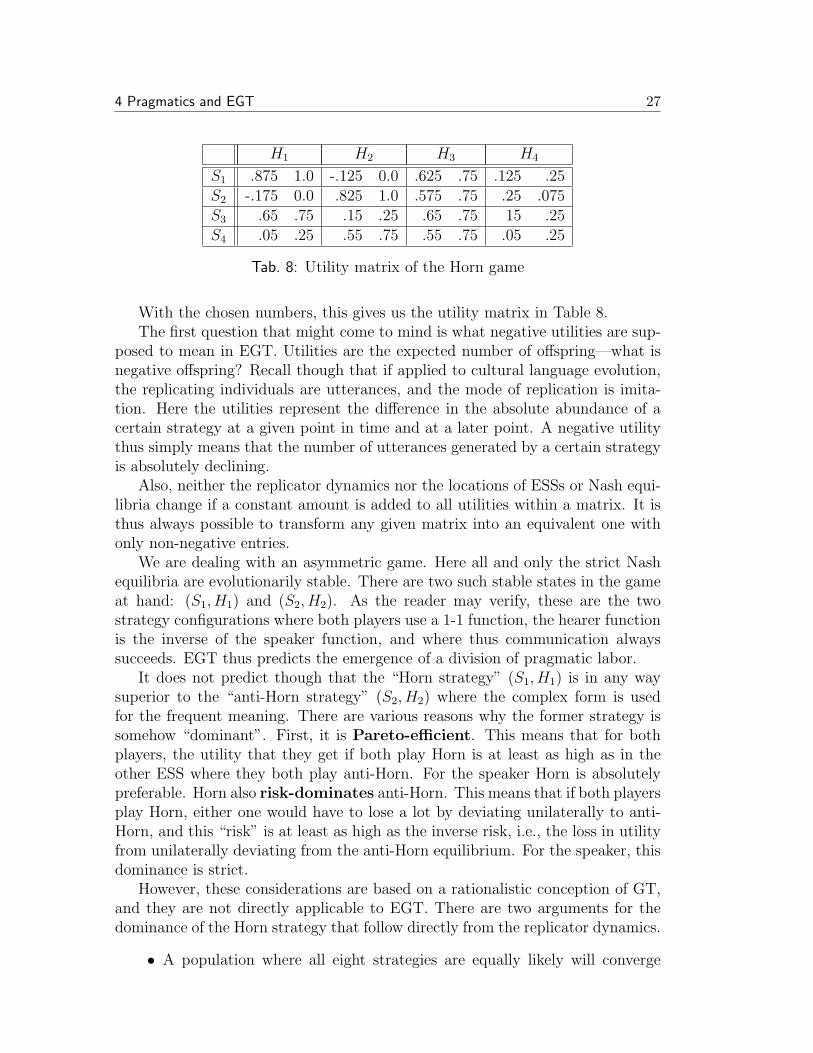
H1 H2 H3 H4
S1 .875 1.0 -.125 0.0 .625 .75 .125 .25S2 -.175 0.0 .825 1.0 .575 .75 .25 .075S3 .65 .75 .15 .25 .65 .75 15 .25S4 .05 .25 .55 .75 .55 .75 .05 .25
Tab. 8: Utility matrix of the Horn game
With the chosen numbers, this gives us the utility matrix in Table 8.The first question that might come to mind is what negative utilities are sup-
posed to mean in EGT. Utilities are the expected number of offspring—what isnegative offspring? Recall though that if applied to cultural language evolution,the replicating individuals are utterances, and the mode of replication is imita-tion. Here the utilities represent the difference in the absolute abundance of acertain strategy at a given point in time and at a later point. A negative utilitythus simply means that the number of utterances generated by a certain strategyis absolutely declining.
Also, neither the replicator dynamics nor the locations of ESSs or Nash equi-libria change if a constant amount is added to all utilities within a matrix. It isthus always possible to transform any given matrix into an equivalent one withonly non-negative entries.
We are dealing with an asymmetric game. Here all and only the strict Nashequilibria are evolutionarily stable. There are two such stable states in the gameat hand: (S1, H1) and (S2, H2). As the reader may verify, these are the twostrategy configurations where both players use a 1-1 function, the hearer functionis the inverse of the speaker function, and where thus communication alwayssucceeds. EGT thus predicts the emergence of a division of pragmatic labor.
It does not predict though that the “Horn strategy” (S1, H1) is in any waysuperior to the “anti-Horn strategy” (S2, H2) where the complex form is usedfor the frequent meaning. There are various reasons why the former strategy issomehow “dominant”. First, it is Pareto-efficient. This means that for bothplayers, the utility that they get if both play Horn is at least as high as in theother ESS where they both play anti-Horn. For the speaker Horn is absolutelypreferable. Horn also risk-dominates anti-Horn. This means that if both playersplay Horn, either one would have to lose a lot by deviating unilaterally to anti-Horn, and this “risk” is at least as high as the inverse risk, i.e., the loss in utilityfrom unilaterally deviating from the anti-Horn equilibrium. For the speaker, thisdominance is strict.
However, these considerations are based on a rationalistic conception of GT,and they are not directly applicable to EGT. There are two arguments for thedominance of the Horn strategy that follow directly from the replicator dynamics.
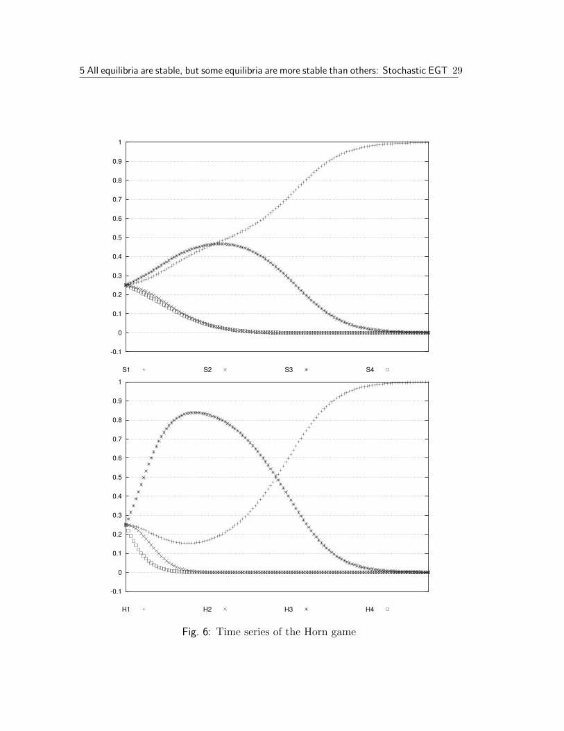
• A population where all eight strategies are equally likely will converge
5 All equilibria are stable, but some equilibria are more stable than others: Stochastic EGT 28
towards a Horn strategy. Figure 6 on the following page gives the timeseries for all eight strategies if they all start at 25% probability. Note thatthe hearers first pass a stage where strategy H3 is dominant. This is thestrategy where the hearer always “guesses” the more frequent meaning—a good strategy as long as the speaker is unpredictable. Only after thespeaker starts to clearly differentiate between the two meanings does H1
begin to flourish.
• While both Horn and anti-Horn are attractors under the replicator dy-namics, the former has a much larger basin of attraction than the latter.We are not aware of a simple way of analytically calculating the ratio ofthe sizes of the two basins, but a numerical approximation revealed thatthe basin of attraction of the Horn strategy is about 20 times as large asthe basin of attraction of the anti-Horn strategy.
The asymmetry between the two ESSs becomes even more apparent when theidealizations “infinite population” and “complete random mating” are lifted. Inthe next sections we will briefly explore the consequences of this.
5 All equilibria are stable, but some equilibria are morestable than others: Stochastic EGT
Let us now have a closer look at the modeling of mutations in EGT. Evolutionarystability means that a state is stationary and resistant against small amounts ofmutations. This means that the replicator dynamics is tacitly assumed to becombined with a small stream of mutation from each strategy to each otherstrategy. The level of mutation is assumed to be constant. An evolutionarilystable state is a state that is an attractor in the combined dynamics and remainsan attractor as the level of mutation converges towards zero.
The assumption that the level of mutation is constant and deterministicthough is actually an artifact of the assumption that populations are infiniteand time is continuous in standard EGT. Real populations are finite, and bothgames and mutations are discrete events in time. So a more fine-grained mod-eling should assume finite populations and discrete time. Now suppose that foreach individual in a population, the probability to mutate towards the strategys within one time unit is p, where p may be very small but still positive. If thepopulation consists of n individuals, the chance that all individuals end up play-ing s at a given point in time is at least pn, which may be extremely small butis still positive. By the same kind of reasoning, it follows that there is a positiveprobability for a finite population to jump from each state to each other statedue to mutation (provided each strategy can be the target of mutation of eachother strategy). More generally, in a finite population the stream of mutations isnot constant but noisy and non-deterministic. Hence there are strictly speaking
5 All equilibria are stable, but some equilibria are more stable than others: Stochastic EGT 29
-0.1
0
0.1
0.2
0.3
0.4
0.5
0.6
0.7
0.8
0.9
1
S1 S2 S3 S4
-0.1
0
0.1
0.2
0.3
0.4
0.5
0.6
0.7
0.8
0.9
1
H1 H2 H3 H4
Fig. 6: Time series of the Horn game
5 All equilibria are stable, but some equilibria are more stable than others: Stochastic EGT 30
no evolutionarily stable strategies because every invasion barrier will eventuallybe overcome, no matter how low the average mutation probability and how highthe barrier is.10
If an asymmetric game has exactly two SNEs, A and B, in a finite populationwith mutations there is a positive probability pAB that the system moves from Ato B due to noisy mutation, and a probability pBA for the reverse direction. IfpAB > pBA, the former change will on average occur more often than the latter,and in the long run the population will spend more time in state B than instate A. Put differently, if such a system is observed at some arbitrary time, theprobability that it is in state B is higher than that it is in A. The exact value ofthis probability converges towards pAB
pAB+pBAas time grows to infinity.
If the level of mutation gets smaller, both pAB and pBA get smaller, butat different pace. pBA approaches 0 much faster than pAB, and thus pAB
pAB+pBA
(and thus the probability of the system being in state B) converges to 1 as themutation rate converges to 0. So while there is always a positive probability thatthe system is in state A, this probability can become arbitrarily small. A stateis called stochastically stable if its probability converges to a value > 0 asthe mutation rate approaches 0. In the described scenario, B would be the onlystochastically stable state, while both A and B are evolutionarily stable. Thenotion of stochastic stability is a strengthening of the concept of evolutionarystability; every stochastically stable state is also evolutionarily stable,11 but notthe other way round.
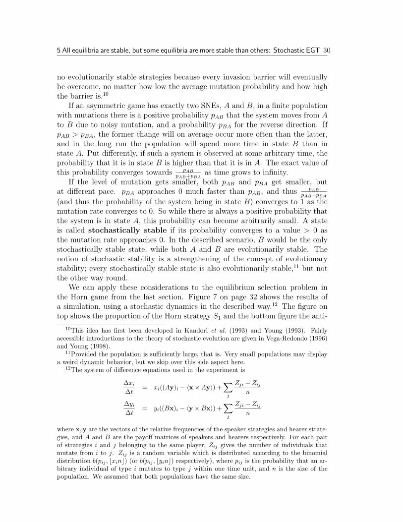
We can apply these considerations to the equilibrium selection problem inthe Horn game from the last section. Figure 7 on page 32 shows the results ofa simulation, using a stochastic dynamics in the described way.12 The figure ontop shows the proportion of the Horn strategy S1 and the bottom figure the anti-
10This idea has first been developed in Kandori et al. (1993) and Young (1993). Fairlyaccessible introductions to the theory of stochastic evolution are given in Vega-Redondo (1996)and Young (1998).
11Provided the population is sufficiently large, that is. Very small populations may displaya weird dynamic behavior, but we skip over this side aspect here.
12The system of difference equations used in the experiment is
∆xi
∆t= xi((Ay)i − 〈x×Ay〉) +
∑j
Zji − Zij
n
∆yi
∆t= yi((Bx)i − 〈y ×Bx〉) +
∑j
Zji − Zij
n
where x,y are the vectors of the relative frequencies of the speaker strategies and hearer strate-gies, and A and B are the payoff matrices of speakers and hearers respectively. For each pairof strategies i and j belonging to the same player, Zij gives the number of individuals thatmutate from i to j. Zij is a random variable which is distributed according to the binomialdistribution b(pij , bxinc) (or b(pij , byinc) respectively), where pij is the probability that an ar-bitrary individual of type i mutates to type j within one time unit, and n is the size of thepopulation. We assumed that both populations have the same size.

5 All equilibria are stable, but some equilibria are more stable than others: Stochastic EGT 31
Horn strategy S2. The other two speaker strategies remain close to zero. Thedevelopment for the hearer strategies is pretty much synchronized.
During the simulation, the system spent 67% of the time in a state witha predominant Horn strategy and only 26% with predominant anti-Horn (theremaining time are the transitions). This seems to indicate strongly that theHorn strategy is in fact the more probable one, which in turn indicates that it isthe only stochastically stable state.
The literature contains some general results about how to find the stochas-tically stable states of a system analytically, but they are all confined to 2×2games. This renders them practically useless for linguistic applications becausehere, even in very abstract models like the Horn game, we deal with more thantwo strategies per player. For larger games, analytical solutions can only be foundby studying the properties in question on a case by case basis. It would take ustoo far to discuss possible solution concepts here in detail (see for instance Young1998 or Ellison 2000). We will just sketch such an analytical approach for theHorn game, which turns out to be comparatively well-behaved.
To check which of the two ESSs of the Horn game are stochastically stable,we have to compare the height of their invasion barriers. How many speakersmust deviate from the Horn strategy such that even the smallest hearer mutationcauses the system to leave the basin of attraction of this strategy and to movetowards the anti-Horn strategy? And how many hearer-mutations would havethis effect? The same questions have to be answered for the anti-Horn strategy,and the results to be compared.
Consider speaker deviations from the Horn strategy. It will only lead to anincentive for the hearer to deviate as well if H1 is not the optimal response to thespeaker strategy anymore. This will happen if at least 50% of all speakers deviatetoward S2, 66.7% deviate towards S4, or some combination of such deviations. Itis easy to see that the minimal amount of deviation having the effect in questionis 50% deviating towards S2.
13
As for hearer deviation, it would take more than 52.5% mutants towards H2
to create an incentive for the speaker to deviate towards S2, and even about 54%of deviation towards H4 to have the same effect. So the invasion barrier alongthe hearer dimension is 52.5%.
Now suppose the system is in the anti-Horn equilibrium. As far as hearerutilities are concerned, Horn and anti-Horn are completely symmetrical, andthus the invasion barrier for speaker mutants is again 50%. However, if morethan 47.5% of all hearers deviate towards H1, the speaker has an incentive todeviate towards S1.
13Generally, if (si, hj) form a SNE, the hearer has an incentive to deviate from it as soonas the speaker chooses a mixed strategy x such that for some k 6= j,
∑i′ xi′uh(si′ , hk) >∑
i′ xi′uh(si′ , hj). The minimal amount of mutants needed to drive the hearer out of theequilibrium would be the minmal value of 1− xi for any mixed strategy x with this property.(The same applies ceteris paribus to mutations on the hearer side.)
5 All equilibria are stable, but some equilibria are more stable than others: Stochastic EGT 32
0
0.1
0.2
0.3
0.4
0.5
0.6
0.7
0.8
0.9
1
Horn
0
0.1
0.2
0.3
0.4
0.5
0.6
0.7
0.8
0.9
1
anti-Horn
Fig. 7: Simulation of the stochastic dynamics of the Horn game
6 Don’t talk to strangers: Spatial EGT 33
In sum, the invasion barriers of the Horn and of the anti-Horn strategy are50% and 47.5% respectively. Therefore a “catastropic” mutation from the latterto the former, though unlikely, is more likely than the reverse transition. Thismakes the Horn strategy the only stochastically stable state.
In this particular example, only two strategies for each player played a rolein determining the stochastically stable state. The Horn game thus behaveseffectively as a 2× 2 game. In such games stochastic stability actually coincideswith the rationalistic notion of “risk dominance” that was briefly discussed above.In the general case, it is possible though that a larger game has two ESSs, butthere is a possible mutation from one equilibrium towards a third state (forinstance a non-strict Nash equilibrium) that lies within the basin of attractionof the other ESS. The stochastic analysis of larger games has to be done on acase-by-case basis to take such complex structures into account.
In standard EGT, as well as in the version of Stochastic EGT discussed here,the utility of an individual at each point in time is assumed to be exactly theaverage utility this individual would get if it played against a perfectly represen-tative sample of the population. Vega-Redondo (1996) discusses another variantof Stochastic EGT where this idealization is also given up. In this model, each in-dividual plays a finite number of tournaments in each time step, and the gainedutility—and thus the abundance of offspring—becomes a stochastic notion aswell. He shows that this model sometimes leads to a different notion of stochas-tic stability than the one discussed here. A detailed discussion of this modelwould lead beyond the scope of this introduction though.
6 Don’t talk to strangers: Spatial EGT
Standard EGT assumes that populations are infinite and each pair of individualsis equally likely to interact. Stochastic gives up the first assumption. The secondassumption is also quite unrealistic. Nowak and May (1992) give it up as well.Instead they assume that players are organized in a spatial structure. A simplemodel for this is a two-dimensional lattice like a chess board. Each player occupiesone position in such a grid and interacts solely with its eight immediate neighbors.The overall utility of each player in each round is the sum of the utilities that itobtains in each of these eight interactions. In the next generation, each positionin the grid adopts the strategy of the player in the immediate environment (theeight neighboring positions and the position in question itself) that obtained thehighest utility.
This kind of deterministic dynamics has a good deal of intrinsic mathematicalinterest because it leads to fascinating self-organizing behavior. Besides, variousstudies with different games and parameters invariably revealed that cooperativebehavior performs much better in a spatial setting than in the standard model orin Stochastic EGT. There is a simple intuitive reason for this. Every individual

6 Don’t talk to strangers: Spatial EGT 34
interacts with its spatial neighbors. The offspring of an individual are also alwayslocated in its immediate spatial proximity. Therefore individuals are likely tofind their siblings or cousins in their environment. In a less metaphorical wayof speaking, in the spatial setting strategies tend to cluster, and each individualis more likely to interact with somebody playing the same strategy than thepopulation average would predict. Therefore those strategies that receive a highpayoff against themselves have an advantage.
Nowak and May’s pioneering paper, as well as most of the work that followedit (see for instance Killingback and Doebeli 1996), use the deterministic dynamicswhereas each individual imitates the strategy with the highest utility in its spatialenvironment. We will use a perhaps more realistic non-deterministic version ofspatial dynamics in the remainder of this section. The qualitative results of thementioned studies remain valid in this setting.
Recall that the utility is a measure for the expected number of offspring. If theoffspring of an individual is distributed evenly over its spatial proximity, each cellin the lattice should adopt a mixed strategy—the combination of the strategies inits neighborhood in the previous generation, weighted according to their utility.We choose a slightly simpler model where each position is occupied by a purestrategy. The probability of adopting the strategy of a particular neighbor (or toretain the current strategy) is proportional to the utility of that neighbor.
This approach is perhaps too simplistic though. Suppose strategy A obtainsa utility of 10 against itself, while B only gets 5 points against itself. Then ahomogeneous A-region should grow faster (because of its higher fitness) than ahomogeneous B-region. This is not covered in the model so far. To remedythis, let us assume that each position can be populated by several individualssimultaneously. They are clones, i.e., they play the same strategy. The denser aposition is populated, the higher is its impact on neighboring fields.
To make this formally precise, let us assume a set of positions pos and asymmetric and irreflexive neighborhood relation n among elements of pos. Thestrategy function st maps positions and time points to a random variable over thestrategy space. Likewise, the density function d maps positions and time pointsto a random variable over positive real numbers. Finally, the fitness function fmaps positions and time points to positive reals as well. Z(a, t) is a normalizationvariable which holds the accumulated weighted fitness of the neighborhood of a.These random variables form a Markov process according to the following updaterules:
f(a, t + 1) =∑
b∈{x:n(a,x)}u(st(a, t), st(b, t))
d(a, t + 1) = d(a, t)× f(a, t + 1)
P (st(a, t + 1) = i) =1
Z(a, t + 1)×
6 Don’t talk to strangers: Spatial EGT 35
C D
C 5 1D 8 2
Tab. 9: Utility matrix for the Prisoner’s Dilemma
∑(b∈{x:n(a,x)}∪{a})∩{x:st(x,t)=i}
d(b, t + 1)× f(b, t + 1)
Z(a, t + 1) =∑
b∈{x:n(a,x)}∪{a}d(b, t + 1)× f(b, t + 1)
It is a nice feature of this version of spatial dynamics that it is a refinementof the standard model. If the neighborhood of each point is identified with theentire set of positions, this dynamics converges towards the replicator dynamicsas the number of positions grows to infinity.
In the sequel we follow Nowak and May (1992) in assuming the two-dimensionallattice structure. Positions are arranged in a 50 × 50 grid. It is interpretedtoroidal. This means that the top row neighbors the bottom row, and likewisefor the leftmost and the rightmost column. Let us first consider the Hawk-and-Dove game discussed above. Recall that the only ESS in the standard model was80% hawks vs. 20% doves. In the spatial setting, the dove strategy fares muchbetter.
Both strategies tend to form clusters. At the boundary between hawk popu-lations and dove populations, hawks have the same advantage as in the classicalsetting. However, areas of dove sub-populations reach a higher density withina cluster than hawk areas because doves against doves have a utility of 3 whilehawks against hawks only have a utility of 1. These two tendencies interact.Depending on the size of the clusters (which varies from generation to genera-tion), the proportion of hawks in the entire population may reach its “classical”share of 80%, but it occasionally drops down to 50% and below. Figure 8 onthe following page shows the relative proportion of hawks in a typical run of asimulation, starting from a state where both strategies are distributed randomlywith equal probability over the range of positions.
Here the divergence from the classical model was only gradual. In case of theprisoner’s dilemma, the spatial model(s) make(s) qualitatively different predic-tions. Recall that in the prisoner’s dilemma, we have two competing strategies,C (“Cooperate”) and D (“Defect”). C playing against C obtains a higher utilitythan D playing against D, but for a given strategy of the opponent, D alwaysyields a higher payoff than C, no matter which strategy the opponent chooses.In technical vocabulary, D strictly dominates C, and therefore D is the onlyNash equilibrium. Since it is a strict Nash equilibrium, it is also an ESS.
Table 9 gives some concrete values that instantiate these preferences.Here the advantage that C-players enjoy if playing against other C-players

6 Don’t talk to strangers: Spatial EGT 36
0
0.2
0.4
0.6
0.8
1
Fig. 8: Proportion of hawks in a spatial Hawk-and-Dove game
(T,A) (T, I) (S, A) (S, I)
(T, A) 3 2 1 0(T, I) 2 1 2 1(S, A) 3 3 1 1(S, I) 2 2 2 2
Tab. 10: Symmetrized game of communication
is so overwhelming that it outweighs the disadvantage that ensues in direct en-counters with defectors. Figure 9 on the following page shows the proportion ofC-players in a simulation using the above utilities. We again started with aninitial state where the strategies were assigned to positions at random with equallikelihood. In this state, there is little clustering, and most individuals interactwith players using the other strategy. In this situation, D fares far better thanC, and it almost takes over the entire space. However, some pockets of C-playerssurvive and form clusters. Due to the high density inside these clusters, theyconstantly increase their size, until they finally occupy almost the entire space.
The selection for cooperative behavior in spatial evolution is of obvious rele-vance for the evolution of communication. We briefly touched upon this issue inconnection with the “game of communication” (see Table 4 on page 17). If wesymmetrize this game, we get the utility matrix in Table 10.
The only ESS here is (S, I), which corresponds to the only strict Nash equi-librium in the asymmetric version. The combination (T, I) is more beneficial forthe hearer though and not worse than the ESS for the speaker. We thus have a

6 Don’t talk to strangers: Spatial EGT 37
0
0.2
0.4
0.6
0.8
1
Fig. 9: Proportion of cooperators in a spatial Prisoner’s Dilemma game
pattern that is similar to the prisoner’s dilemma. The ensuing spatial evolutionis also similar. Starting from a random state, the ESS (S, I) quickly gains dom-inance and drives the other strategies close to extinction. In most simulations,some small clusters of the cooperative strategy (T, A) survive though. Theseclusters thrive and increase their size until they reach a stable shape. Under thegrid structure used here, stable structures are squares or rectangles which arealmost squares. The snapshots in figure 10 on the following page display thestate of the system in the first, 11th, 25th, 100th, 200th and 500th generation.The strategy (S, I) is indicated by white squares and all other strategies by blacksquares. (T, I) and (S, A) die out after less than 30 generations; after that blacksquares just indicate (T, A).
Interestingly, the equivalence between an asymmetric game and its sym-metrized version breaks down under spatial evolution. In an asymmetric spatialcompetition, where players from both populations share one position in the lat-tice and each individual interacts with the individuals from the other populationin its neighborhood, the classical ESS (S, I) turns out to drive the cooperativestrategies T and A to extinction. The time series of the frequencies of the strate-gies in a simulation of the two-population spatial competition is given in figure 11on page 39.
This result is not surprising once one realizes that only the column playertruly benefits from cooperative behavior. A two-population symbiosis can onlyemerge if both populations would benefit.
There are no applications of spatial EGT to linguistic problems so far that
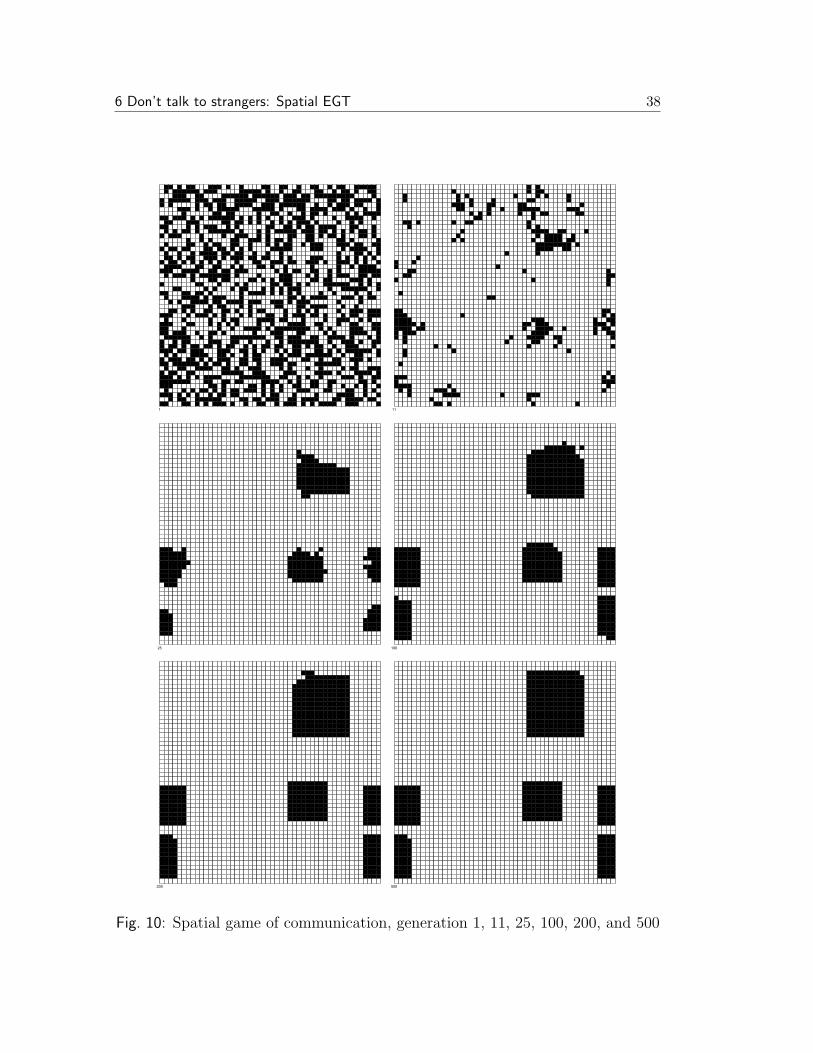
6 Don’t talk to strangers: Spatial EGT 38
1 11
25 100
200 500
Fig. 10: Spatial game of communication, generation 1, 11, 25, 100, 200, and 500
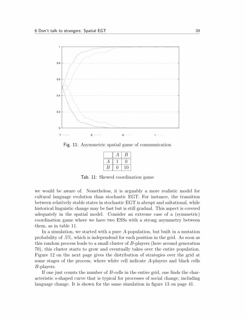
6 Don’t talk to strangers: Spatial EGT 39
0
0.2
0.4
0.6
0.8
1
T S A I
Fig. 11: Asymmetric spatial game of communication
A B
A 1 0B 0 10
Tab. 11: Skewed coordination game
we would be aware of. Nonetheless, it is arguably a more realistic model forcultural language evolution than stochastic EGT. For instance, the transitionbetween relatively stable states in stochastic EGT is abrupt and saltational, whilehistorical linguistic change may be fast but is still gradual. This aspect is coveredadequately in the spatial model. Consider an extreme case of a (symmetric)coordination game where we have two ESSs with a strong asymmetry betweenthem, as in table 11.
In a simulation, we started with a pure A-population, but built in a mutationprobability of .5%, which is independend for each position in the grid. As soon asthis random process leads to a small cluster of B-players (here around generation70), this cluster starts to grow and eventually takes over the entire population.Figure 12 on the next page gives the distribution of strategies over the grid atsome stages of the process, where white cell indicate A-players and black cellsB-players.
If one just counts the number of B-cells in the entire grid, one finds the char-acteristic s-shaped curve that is typical for processes of social change, includinglanguage change. It is shown for the same simulation in figure 13 on page 41.

6 Don’t talk to strangers: Spatial EGT 40
50 75
80 90
100 110
Fig. 12: Skewed coordination game, generation 50, 75, 80, 90, 100, 110
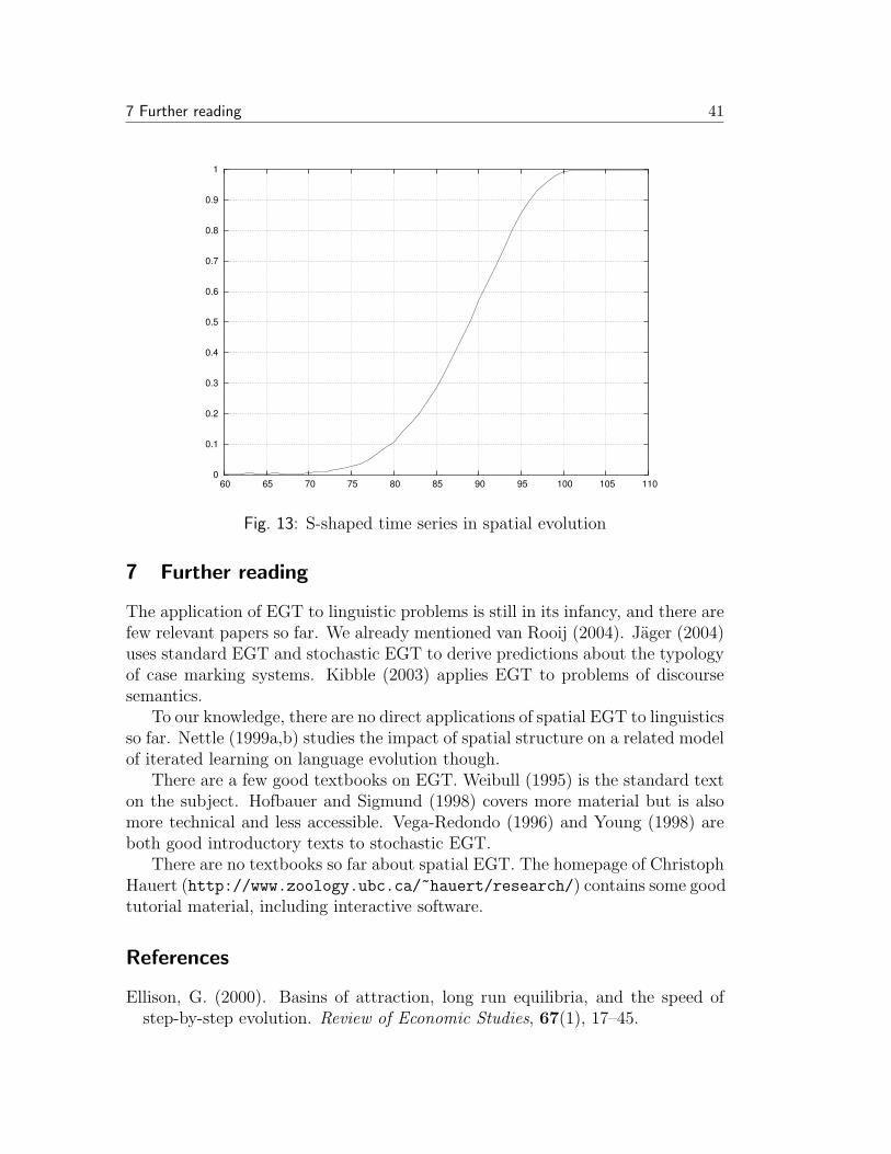
7 Further reading 41
0
0.1
0.2
0.3
0.4
0.5
0.6
0.7
0.8
0.9
1
60 65 70 75 80 85 90 95 100 105 110
Fig. 13: S-shaped time series in spatial evolution
7 Further reading
The application of EGT to linguistic problems is still in its infancy, and there arefew relevant papers so far. We already mentioned van Rooij (2004). Jager (2004)uses standard EGT and stochastic EGT to derive predictions about the typologyof case marking systems. Kibble (2003) applies EGT to problems of discoursesemantics.
To our knowledge, there are no direct applications of spatial EGT to linguisticsso far. Nettle (1999a,b) studies the impact of spatial structure on a related modelof iterated learning on language evolution though.
There are a few good textbooks on EGT. Weibull (1995) is the standard texton the subject. Hofbauer and Sigmund (1998) covers more material but is alsomore technical and less accessible. Vega-Redondo (1996) and Young (1998) areboth good introductory texts to stochastic EGT.
There are no textbooks so far about spatial EGT. The homepage of ChristophHauert (http://www.zoology.ubc.ca/~hauert/research/) contains some goodtutorial material, including interactive software.
References
Ellison, G. (2000). Basins of attraction, long run equilibria, and the speed ofstep-by-step evolution. Review of Economic Studies, 67(1), 17–45.
7 Further reading 42
Gould, S. J. (2002). The Structure of Evolutionary Theory. Harvard UniversityPress.
Hofbauer, J. and Sigmund, K. (1998). Evolutionary Games and Population Dy-namics. Cambridge University Press, Cambridge (UK).
Horn, L. (1993). Economy and redundancy in a dualistic model of natural lan-guage. In S. Shore and M. Vilkuna, editors, 1993 Yearbook of the LinguisticAssociation of Finland, pages 33–72. SKY.
Jager, G. (2004). Evolutionary Game Theory and typology: a case study.manuscript, University of Potsdam and Stanford University, available fromwww.ling.uni-potsdam.de/˜jaeger/games dcm.pdf.
Kandori, M., Mailath, G., and Rob, R. (1993). Learning, mutation, and long-runequilibria in games. Econometrica, 61, 29–56.
Kibble, R. (2003). A framework for modelling evolutionary stable strategiesin discourse semantics. In P. Dekker and R. van Rooij, editors, Proceedingsof the Fourteenth Amsterdam Colloquium, pages 27–32. ILLC, University ofAmsterdam.
Killingback, T. and Doebeli, M. (1996). Spatial evolutionary game theory: Hawksand doves revisited. Proceedings of the Royal society of London, 263, 1135–1144.
Kroch, A. (2000). Syntactic change. In M. Baltin and C. Collins, editors, TheHandbook of Contemporary Syntactic Theory, pages 699–729. Blackwell Pub-lishers, Oxford.
Labov, W. (1972). Sociolinguistic patterns. University of Pennsylvania Press,Philadelphia.
Maynard Smith, J. (1982). Evolution and the Theory of Games. CambridgeUniversity Press, Cambridge (UK).
Nettle, D. (1999a). Is the rate of linguistic change constant? Lingua, 108,119–136.
Nettle, D. (1999b). Using social impact theory to simulate language change.Lingua, 108, 95–117.
Nowak, M. A. and May, R. M. (1992). Evolutionary games and spatial chaos.Nature, (359), 826–829.
Nowak, M. A., Komarova, N. L., and Niyogi, P. (2002). Computational andevolutionary aspects of language. Nature, 417, 611–617.
Selten, R. (1980). A note on evolutionarily stable strategies in asymmetric animalconflicts. Journal of Theoretical Biology, 84, 93–101.
Taylor, P. and Jonker, L. (1978). Evolutionarily stable strategies and game dy-namics. Mathematical Biosciences, 40, 145–156.
van Rooij, R. (2003). Being polite is a handicap: Towards a game theoreticalanalysis of polite linguistic behavior. In M. Tennenholtz, editor, Proceedings ofthe 9th conference on Theoretical aspects of rationality and knowledge. ACMPress, New York.
van Rooij, R. (2004). Signalling games select Horn strategies. Linguistics and
7 Further reading 43
Philosophy, 27, 493–527.Vega-Redondo, F. (1996). Evolution, Games, and Economic Behaviour. Oxford
University Press.Weibull, J. W. (1995). Evolutionary Game Theory. The MIT Press.Young, H. P. (1993). The evolution of conventions. Econometrica, 61, 57–84.Young, H. P. (1998). Individual Strategy and Social Structure. An Evolutionary
Theory of Institutions. Princeton University Press.Zahavi, A. (1975). Mate selection — a selection for a handicap. Journal of
Theoretical Biology, 53, 205–213.