Embed Size (px)
Citation preview

Liquefaction Guidelines April 9th, 2014
Utah Chapter EERI Short Course
Evaluation and Mitigation of Liquefaction Hazard for Engineering Practice
Wednesday April 9th
, 2014
Maverik Center, West Valley, Utah
W.D. Liam Finn, University of British Columbia, Vancouver, Canada
Invited Instructor
This lecture material is an updating and extension of guidelines originally developed for the British Columbia Schools Seismic Retrofit Program by
W.D. Liam Finn and Jason Dowling, University of British Columbia
A. Wightman, BGC Engineering, Vancouver
John Sherstobitoff, Ausenco Ltd, Vancouver

Table of Contents Page: (ii)
Liquefaction Guidelines April 9th, 2014
Table of Contents
Chapter Section Title Page
Executive Summary (iv)
Introduction (v)
1.0 Site Investigation 1
1.1 Geology 1
1.2 Geotechnical Site Investigation Techniques 1
1.3 Scope of Investigations 4
2.0 Evaluation of Liquefaction Potential 6
2.1 Introduction 6
2.2 Simplified method for seismic stress analysis 6
2.3 Rigorous Stress Analysis 8
2.4 SPT-Based Resistance 9
2.5 CPT-Based Resistance 13
2.6 Vs-Based Resistance 16
2.7 Liquefaction Assessment Software 18
2.8 Simplified Method using Probabilistic Accelerations 19
2.9 Weighted Residual Method 20
2.10 Magnitude Deaggregation Method 22
3.0 Liquefaction or Cyclic Failure of Fine-Grained Clays and Plastic Silts 27
3.1 Simplified Stress Analysis for Plastic Soils 27
3.2 Resistance Capacity, CRR 28
3.3 Estimating CRR from Su Profile 29
3.4 Method 3 30
3.5 Effect of Initial Static Shear Stress 30
3.6 Consequences of Cyclic Failure in Plastic Soils 31
4.0 Consequences of Liquefaction in Terms of Ground Displacements 32
4.1 General 32
4.2 Youd et al. (2002) Model 32
4.3 Lateral Displacements using Magnitude-Distance Deaggregation 35
4.4 Idriss and Boulanger (2008) Model 37
4.5 Zhang et al. (2004) Model 38
4.6 Vertical Settlements due to Consolidation after Liquefaction 40
4.6.1 Ishihara & Yoshimine (1992) Model 40
5.0 Structural Considerations 42
5.1 General 42

Table of Contents Page: (iii)
Liquefaction Guidelines April 9th, 2014
Chapter Section Title Page
5.2 Assessment 42
5.2.1 Existing Information 42
5.2.2 Foundations located in non liquefiable crust 43
5.2.3 Foundations in liquefiable soil 44
5.2.4 Allowable structure drifts due to liquefaction effects 44
5.2.5 Lateral soil spreading effects 45
5.2.6 Differential vertical settlement effects 47
5.2.7 Connections 48
6.0 Remedial Options 49
6.1 General 49
6.2 Soil Remediation 49
6.3 Structural Remediation 50
6.3.1 For inadequate punching shear capacity 50
6.3.2 For excessive lateral spread effects 50
6.3.3 For excessive differential vertical settlements 50
6.4 Enhanced Performance Retrofit 50
7.0 Closing the Loop: Reconciling Geotechnical Demands with Performance Criteria 52
7.1 Performance Limits for School 52
7.2 Estimation of Total Drift 53
7.3 Geotechnical Engineer Input 53
7.4 Retrofit Details 55
7.5 Finished Project 56
8.0 References 57

Executive Summary Page: (iv)
Liquefaction Guidelines April 9th, 2014
Executive Summary
Guidelines for Evaluating Liquefaction Potential and Consequences
These guidelines provide state of the art information and guidance on
Site Investigation
Evaluation of Liquefaction Potential
Consequences of Liquefaction in terms of Ground Displacements
Mitigation of Liquefaction effects by structural retrofits and geotechnical measures

Executive Summary Page: (v)
Liquefaction Guidelines April 9th, 2014
Introduction
The 1964 earthquakes in Niigata and Alaska caused devastating damage to structures and all kinds of
infrastructure as a result of widespread liquefaction. Reconstruction required a good understanding of the
mechanics of liquefaction but little was known about liquefaction at the time. Major research programs
were initiated by the Universities of California and Tokyo to support safe reconstruction and both made
significant and lasting contributions to the evaluation of the potential for the triggering of liquefaction and
quantifying the effects of liquefaction in terms of lateral spreading, settlement and slope failures.
In the beginning the study of liquefaction was based on cyclic loading tests of reconstituted samples.
These tests were very useful for defining the mechanics of liquefaction and giving insight into potential
consequences but it was quickly realized that such samples were not representative of field conditions
and therefore could not be relied upon to assess the liquefaction potential in the field. Attention turned to
the possibility of using in situ penetration tests to assess the density and hence the resistance of soils in
situ to liquefaction. These studies have resulted in the development of Liquefaction Assessment Charts
based on SPT-N, CPT-qc and for soils that are difficult to penetrate, charts based on shear wave velocity,
Vs. In the early days, site response analysis was not a viable option, so Seed and Idriss (1971)
developed a simplified method for estimating the cycles of uniform stress representative of the actual
shaking intensity of the earthquake. This approach, despite advances in computational capacity, is still
very widely used.
The approach described above is a deterministic approach based on a specified design earthquake and
an associated peak ground acceleration. At present a number of codes specify site hazard
probabilistically, mostly a hazard with an exceedance rate of 2% in 50 years. To deal with probabilistic
ground motions, the approach to evaluating liquefaction hazard using the simplified method requires
some modifications.
These course notes describe both the deterministic and probabilistic approaches to the evaluation of
liquefaction potential and its consequences. The simplified method was developed for sands and
cohesionless silts. It has become clear, especially from field data from recent Turkish earthquakes that
fine grained plastic soils can also suffer strength loss and stiffness degradation under cyclic loading. The
course notes describe how these soils can be evaluated in the simplified framework when necessary
modifications are made.
Finally the course notes review remediation options and stress the importance of evaluating the potential
of either structural or geotechnical retrofits. Cases where structural retrofits are cheaper are not
uncommon for smaller buildings. The course ends with a “Closing the Loop” example, showing the value
of informed interaction between Structural and Geotechnical Engineers.

Site Investigation Page: 1
Liquefaction Guidelines April 9th, 2014
1.0 Site Investigation
1.1 Geology
Desk studies should include reference to surficial geological maps and reports, supplemented by
air photo interpretation and ground truthing where appropriate. Liquefaction hazard maps are also
useful sources of information. The aim should be to identify areas underlain by normally
consolidated deposits of Pleistocene and Holocene age, as well as regions of flooding and/or
high ground water levels. It is important to identify any areas of filled ground, especially in coastal
or riverine environments where loose fills might extend below the water line.
1.2 Geotechnical Site Investigation Techniques
The resistance of soil deposits to liquefaction is usually determined using in-situ testing
comprising one or more of penetration tests, such as the Standard Penetration Test (SPT) or the
Cone Penetration Test (CPT), or measurement of shear wave velocity, Vs. The CPT may include
measurement of pore-water pressure, u, (CPTu) or seismic shear wave velocity, Vs. For the case
of soft silty clays and low plastic silts, although these types of soils may not liquefy in the
traditional sense, earthquake shaking can often exceed cyclic strength and produce significant
cyclic softening and deformation response. This is often best evaluated using undisturbed
sampling and laboratory testing supported by in-situ vane shear testing and/or CPTu.
(1) Standard Penetration Testing
The original work to characterize liquefaction resistance was correlated to the Standard
Penetration Test (SPT). In more recent years the Cone Penetration Test (CPT) has come
into favor because of its greater level of standardization and repeatability, given suitable
soils free of gravels and cemented layers. The SPT may often still be the method of
choice, especially when the recovery of samples for laboratory index testing forms an
important part of the evaluation. However push samples can now be retrieved by the
CPT. When using SPT to characterize liquefaction resistance it is important that the
testing be carried out according to ASTM D-606 to ensure repeatable, reliable results.
Some of the standard features of reliable SPT testing are listed below, starting with the
drilling of the test hole.
Test holes should be drilled using techniques that minimize disturbance of the bottom
of the hole prior to sampling. When drilling below the water table, this usually requires
using rotary drilling with mud as a drilling fluid to stabilize the walls and base of the
hole. The drill bit used should not jet drilling fluid vertically downwards as this would
disturb the base of the hole. A modified tricone bit that jets laterally or upwards is the
preferred method. Under no circumstances should air-flush, hollow stem augers, or
vibratory drilling methods be used when reliable SPT measurements are required
In order to be sure that SPT sampling is being carried out in undisturbed soil beyond
the base of the hole, it is good practice for the supervising engineer to record the
depth drilled prior to sampling and also to record and compare this with the depth to

Site Investigation Page: 2
Liquefaction Guidelines April 9th, 2014
the tip of the split spoon sampler, to ensure that there has been no caving or heaving
of the base of the hole. Collapse of the base of the hole can be a problem especially
in loose fine sands. Adopting as standard practice the slow withdrawal of the drill
string, while at the same time maintaining a head of drill mud in the hole at the
ground level or top of the mud pan, will usually solve heave and caving at the base of
the hole.
The SPT test procedure should include a record of the type of hammer used, i.e
automatic or manual drop, style of hammer (donut or safety), number of wraps on the
cathead, if manual, dimensions of the sampling rod string (Aw, HW, Bw etc.), and the
details of the split spoon. In the latter case it is important for the supervising engineer
to record whether or not the split spoon is designed to accommodate a split liner, and
if so whether or not a liner is being used. All drill rod joints should be wrenched tight.
SPT test has the ability to recover a soil sample for inspection and testing. This is
often problematic in loose fine sands, however. Sample recovery can be improved by
making sure that the split spoon head assembly contains a fully functioning ball
valve, with vent holes above, to seal off the sample from any out of balance pressure
from dill mud within the rod string as the sampler is withdrawn from the test hole. The
use of a plastic sand catcher in the tip of the spoon, augmented with a loose wrap of
cling film on its upper surface, is also recommended to enhance sample recovery in
loose ground.
One of the most important variables in SPT testing is the amount of energy delivered to
the drill string by the falling hammer. Research in the mid-1980s determined that the
average North American SPT procedures resulted in energy input to the rod string below
the hammer anvil amounted to 60% of theoretical maximum potential energy of a 140 Lb.
hammer falling 30 inches. Some regional and national variations were determined, and
the profession adopted a “Standard” rod energy ratio of 60% for correlation of liquefaction
field performance and standardization of data from different drill rigs and hammer
assemblies. The routine use of instrumentation to measure the energy delivered to the
SPT rod string, at sites with liquefaction potential, is strongly recommended in preference
to the use of generic correction factors such as those given by Seed et al. (1985). The
equipment and expertise needed to carry out such tests during drilling and sampling are
now available.
The SPT test is most reliable when used in sands and silty sands, but on occasion is
used to estimate the liquefaction resistance of gravelly soils. When this is the case the
recording of incremental 1” blow counts is recommended. The blows are counted for
each 1” of penetration, rather than in 6” increments used for standard testing. Comparing
the variability within the typical 12 to 18 such values, usually by plotting cumulative
penetration versus blow count and noting changes in slope, can enable the engineer to
estimate where the penetration resistance has been influenced by the coarse fraction of
the sample interfering with the sampler. A more reliable blow count, more representative
of only the sand fraction can usually be estimated from such data sets, by extrapolating a
short interval measurement to an equivalent 12-inch penetration resistance. This
technique is usually most applicable to soils with at least 50% passing the No. 4 sieve.

Site Investigation Page: 3
Liquefaction Guidelines April 9th, 2014
Additional guidance is given by Andrus and Youd (1987), and Vallee and Skryness
(1980).
(2) Cone Penetration Testing
There are several reputable cone contractors available and the industry can now be
considered mature and reliable. The advantage of using CPT equipment for liquefaction
assessments is that it provides a continuous profile with depth, and so is less likely to
miss thin layers of loose or fine grained materials which can have major influence on
liquefaction and post-liquefaction performance. Another advantage of the CPT method is
its repeatability and standardization. But even so there are things to which the
supervising engineer should pay close attention. The size and type of CPT tip should be
noted and recorded. There are two different sizes in common use, a 10 sq.cm tip and a
15 sq.cm tip. The capacity and sensitivity of the cone tip should be selected with care so
as not to use too high a capacity cone in very soft soils and vice-versa. The location of
the pore pressure sensor and attention to the details of its saturation are very important.
In cases where the water table is not close to the ground surface the pore pressure
sensor can become de-saturated on the initial push. Sometimes it is an advantage to
make the cone push in two stages, the first one without a pore pressure tip, or with a
blank tip, to ream out the hole and allow rapid deployment of a fully saturated tip down to
the water table.
A disadvantage of CPT is the lack of a soil sample and the uncertainty associated with
soil classification and particularly with the determination of fines content. Several soil type
interpretation correlations with CPT have been developed in recent years and there is still
ongoing research on this topic. Some of the more recent versions of CPT interpretation
methods are discussed in Robertson (2010). It is recommended that reliance not be
placed totally on such techniques, especially for estimating fines content, so that any
CPT investigation program should be accompanied by a minimum of one sampled boring
with good sample recovery that enables laboratory testing for grain size, fines content,
water content and plasticity. Push samples can be recovered near the CPT location using
the cone to push the samples. Experience has shown that the correlation of fines content
with the cone parameter, Ic, is problematic. Even site-specific correlations, developed
using side by side SPT borings and CPT, cannot always be used with confidence at other
locations on the same site with ostensibly similar geology.
(3) Shear Wave Velocity Measurements
The ability of a soil to transmit shear waves is related to density and effective confining
stress. Shear wave velocity determined in-situ with geophysical techniques is a small
strain parameter that might be related to the small threshold strains which are needed to
trigger liquefaction (Dobry and Abdoun 2011). There is therefore a correlation between
shear wave velocity and liquefaction triggering stresses, but it tends to be somewhat
subdued in comparison to CPT and SPT based correlations. The most common methods
for determination of shear wave velocity are down-hole, cross-hole, and non-invasive
surface methods such as shear wave refraction, SASW, and MASW. The seismic CPT is

Site Investigation Page: 4
Liquefaction Guidelines April 9th, 2014
a variant of the down-hole method. There are also up-hole techniques that are derived
from oil well logging technology which tend to be expensive and are used more for very
deep holes.
(4) Vs from Ambient Motions
An innovative new method, based on ambient vibration measurements, has been
developed for determining the shear wave velocity profile of a site to provide a more
economic approach to Site Class Identification by Vs30. The recorded motions are
inverted using a Monte Caro technique to give the best estimate of the velocity profile.
The efficacy of this derived S in evaluating liquefaction potential will be illustrated later.
(5) Undisturbed Sampling
The evaluation of the earthquake behavior of saturated clays and plastic silts requires an
understanding of undrained strength and in-situ states of stress and stress history (Idriss
and Boulanger, 2008). It is often necessary to obtain high quality undisturbed samples for
laboratory testing. Undisturbed sampling of clayey silts and silty clays for laboratory
testing is best done using thin-walled tubes and a fixed piston sampler. A discussion of
the factors involved in sampling and testing of fine grained soils for purposes of
determining shear strength and earthquake resistance is given in the works of Ladd and
DeGroot (2003), DeGroot and Ladd (2012), and Idriss and Boulanger (2008).
(6) In-Situ Shear Strengths of Fine-Grained Soils
To aid in the determination of undrained strength and stress history (OCR) it is common
to determine undrained strength by in-situ methods. Although there are empirical
correlations of undrained strength with CPT cone tip resistance, qt, the range of
uncertainty is significant, with cone factor Nkt varying typically between 10 and 18. A
preferred in-situ testing procedure is to use a downhole vane with controlled rate of
loading at the surface, such as a Nilcon vane borer or an electric down-hole vane. High
quality measurements of undrained strength obtained in this manner can be used to
develop site-specific cone calibrations if necessary on larger projects.
1.3 Scope of investigations
The extent of site investigations needed to establish the likely performance of school buildings in
potentially liquefiable ground may vary considerably from site to site, to the degree that no one
scope of work fits all cases. Things to consider are the layout of school buildings in plan, the
presence of any sloping ground or deep open ditches and drainage canals, or river banks. In
general a phased approach to site investigations is recommended, with a minimum of three test
locations spaced strategically around the facilities as the first stage. If significant liquefaction
issues are identified, and ground conditions are not uniform, then additional investigation may be
appropriate. The structural engineer assessing school retrofit requirements is usually interested in
knowing the potential for differential movements, both vertically and horizontally. Assessment of
this is influenced by the depth, variability and continuity of potentially liquefiable materials, as well

Site Investigation Page: 5
Liquefaction Guidelines April 9th, 2014
as the types of foundations at the school. Often a suitable strategy in the Fraser Delta area, in the
absence of prior information, is to use the first test hole to explore to a depth of about 30 m, or at
least 5 m of penetration into non-liquefiable soils, and then select the depth of subsequent test
holes to identify variability and continuity of problematic zones across the site. The first test hole
or CPTu can be used to determine a shear wave velocity profile for subsequent use in one or
more of site classification, site response modeling, and liquefaction triggering assessments.
A good example of how knowledge of spatial heterogeneity can affect an assessment of
liquefaction performance of a building is given in Idriss and Boulanger (2008), Chapter 4.
Evaluation of Liquefaction Potential Page: 6
Liquefaction Guidelines April 9th, 2014
2.0 Evaluation of Liquefaction Potential
2.1 Introduction
Guidelines are presented for assessing the potential for triggering liquefaction and for estimating
post-liquefaction lateral spreading displacements and settlements. Unfortunately these are
transitional guidelines because an US NRC committee entitled the National Research Council
Committee on State of the Art and Practice in Earthquake Induced Liquefaction Assessment will
start work to investigate the current status of research and practice for assessing liquefaction
potential and to formulate a generally acceptable state of practice. It is hoped that their report will
resolve the controversy over the relative merits of the Idriss and Boulanger (2008) and the Cetin
et al. (2004) approaches for evaluating liquefaction potential that has troubled the profession over
the last few years.
The generally accepted state of practice for assessing the potential for triggering liquefaction is
set out in Youd et al. (2001). EERI published a monograph by Idriss and Boulanger in 2008
entitled “Soil Liquefaction during Earthquakes” which conducted a global review of research and
practice up to 2007 and made new recommendations for evaluating the triggering of liquefaction.
In these tentative guidelines, the Youd et al. (2001) and the Idriss and Boulanger (2008)
procedures are presented in parallel. This selection is based on the assumption that eventually
Idriss and Boulanger (2008) will be substantially adopted as good practice.
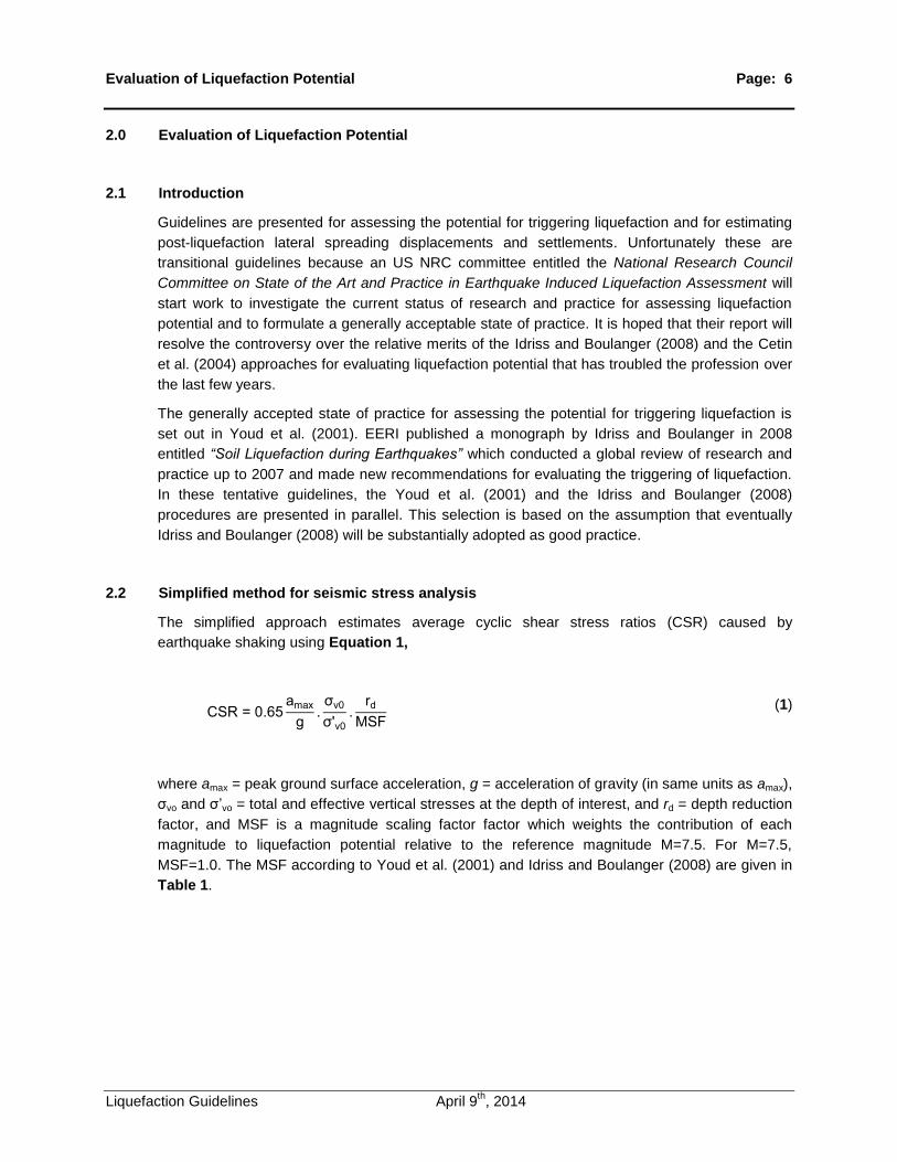
2.2 Simplified method for seismic stress analysis
The simplified approach estimates average cyclic shear stress ratios (CSR) caused by
earthquake shaking using Equation 1,
CS 0.6 amax
g. 0
0.
rd
S
(1)
where amax = peak ground surface acceleration, g = acceleration of gravity (in same units as amax),
vo and ’vo = total and effective vertical stresses at the depth of interest, and rd = depth reduction
factor, and MSF is a magnitude scaling factor factor which weights the contribution of each
magnitude to liquefaction potential relative to the reference magnitude M=7.5. For M=7.5,
MSF=1.0. The MSF according to Youd et al. (2001) and Idriss and Boulanger (2008) are given in
Table 1.

Evaluation of Liquefaction Potential Page: 7
Liquefaction Guidelines April 9th, 2014
Table 1. Magnitude Scaling Factors, MSF
NCEER Youd et al. (2001)
Idriss and Boulanger (2008)
S 10
.
w . 6
S min of [6. exp w
⁄ 0.0 ] or 1.
The two sets of factors are plotted as a function of magnitude in Figure 1. There is significant
difference between the two sets of MSF. Other things being equal, the Idriss and Boulanger
(2008) MSF will lead to much larger Cyclic Stress Ratios, (CSR), for smaller earthquake
magnitudes than Youd et al. (2001) does..
Figure 1. Comparison of Youd et al. (2001) and Idriss and Boulanger (2008) Magnitude
Scaling Factors
Depth reduction factors, rd for use with Youd et al. (2001) and Idriss and Boulanger (2008)
procedures for evaluating the triggering of liquefaction are given in Table 2.

Evaluation of Liquefaction Potential Page: 8
Liquefaction Guidelines April 9th, 2014
Table 2. Depth deduction factors for use with Youd et al. (2001) and Idriss and Boulanger
(2008) procedures for predicting liquefaction triggering
NCEER Youd et al. (2001)
Idriss and Boulanger (2008)
rd 1 0. 11 0. 0.0 0 0.001 1.
1 0. 11 0. 0.0 0.006 0 1. 0.001 1
rd exp w
where
1.01 1.1 6sin (
11. .1 )
0.016 0.01 sin (
11. .1 )
with z in metres and limited to a maximum
depth of 20m, below which the use of site
specific response analysis is recommended.
2.3 Rigorous Stress Analysis
A more rigorous approach to computing the seismic shear stresses is to use site response
analysis. The analysis should be performed with a suite of input motions scaled to the uniform
hazard spectrum for the site with an exceedance rate of 2% in 50 years. The number of input
motions required depends on the number of different types of sources with about 10 motions per
source type. The seismicity British Columbia is driven by 3 types of sources; crustal, subcrustal
and subduction. The peak cyclic shear stress amplitudes at the depths of interest should be taken
as the averages of the peak values produced by the site response analyses. While this is a more
accurate method of getting site specific shear stresses, it was not the procedure followed in
establishing the liquefaction assessment charts which ultimately form the basis for the
assessment of liquefaction potential. Sometimes the differences are substantial.
Recently Boulanger et al. (2014) formulated the procedure for assessing liquefaction potential as
follows:
“The formal assessment of liquefaction at a site using the simplified procedure should be based
on the amax that is estimated to develop in the absence of soil softening or liquefaction.”

Evaluation of Liquefaction Potential Page: 9
Liquefaction Guidelines April 9th, 2014
2.4 SPT-Based Resistance
SPT-based liquefaction evaluation procedures are based on the correlation of liquefaction
resistance to the corrected standard penetration resistance of the soil. The correlation
recommended by Youd et al. (2001) is shown in Figure 2. The correction process involves the
application of a number of correction factors to the field measured SPT resistance. The
necessary corrections are described in Youd et al. (2001). It is important to correct the SPT
measurements for overburden pressure and non-plastic fines content. The overburden correction
factor, CN, is given in Table 3 and the fines correction procedures specified by Youd et al. (2001)
and Idriss and Boulanger (2008) are shown in Table 4.
Figure 2. Liquefaction assessment hart based on normalized SPT-N values (Youd et al.
2001)

Evaluation of Liquefaction Potential Page: 10
Liquefaction Guidelines April 9th, 2014
Table 3. Overburden corrections for measured SPT-N values
NCEER Youd et al. (2001)
Idriss and Boulanger (2008)
Either of the equations below may be used for
overburden correction.
C √pa
0
C . (1. 0
pa
)⁄
C ( 0
pa
)
0. 0.0 6 √ 1 60
1.
Note: Since (N1)60 is required to compute CN
(on which (N1)60 depends), iteration is required.
Table 4. Clean Sand Corrected SPT Resistance (Correction for fines content)
Youd et al. (2001)
Idriss and Boulanger (2008)
1 60,cs 1 60
where
{
0 , C %
exp 1. 6 1 0
C , % C %
0 , C %
{
1.0 , C %
0. C
1.
, % C %
1. , C %
and FC is in percent.
1 60,cs 1 60 1 60
where
1 60 exp [1.6 .
C 0.01 (
1 .
C 0.01)
]
and FC is in percent.

Evaluation of Liquefaction Potential Page: 11
Liquefaction Guidelines April 9th, 2014
The equations for calculating the cyclic resistance ratios, CRR @ ϭ 1atm as functions of (N1)60,cs
using the Youd and Idriss& Boulanger procedures, are given in Table 5.
Table 5. Cyclic Resistance Ratios (CRR) for M = 7.5 and ϭ’vo = 1atm
NCEER Youd et al. (2001)
Idriss and Boulanger (2008)
C 1atm 1
1 60,cs 1 60,cs
1
0
10 1 60,cs
1
00
C 1atm exp 1 60,cs
1 .1 (
1 60,cs
1 6)
( 1 60,cs
.6)
( 1 60,cs
. )
. ]
The Youd et al. (2001) and Idriss and Boulanger (2008) procedures require that the value of CRR
be adjusted to account for the in- situ vertical effective stress using the relationships.
C @ C @ ’ 1atm (2)
The expressions for K are shown in Table 6.
Table 6. Overburden stress correction factor, Kσ, for SPT- and CPT-Based methods
NCEER Youd et al. (2001)
Idriss and Boulanger (2008)
min{( 0
pa
)
f 1
1.0
where f = 0.7-0.8 for Dr = 40-60% and f = 0.6-
0.7 for Dr = 60-80%.
min {1-C ln (
0
pa)
1.1
where
C 1
1 . . √ 1 60
0. for S T
C 1
1 . . √qc1 0. 6
0. for C T

Evaluation of Liquefaction Potential Page: 12
Liquefaction Guidelines April 9th, 2014
The correlation of C for ’ 1atm and magnitude M=7.5 with normalized SPT-N is shown in
Figure 3. Both the Youd et al. (2001) and Idriss and Boulanger (2008) procedures give very
similar results for M=7.5 when MSF=1.0. However for M=6.0, the different approaches to scaling
factors result in significantly different CRR correlations with (N1)60 .as shown in Figure 4. The
impact of the different scaling factors will be noticeable primarily for sources with Mma 6.5.
Figure 3. Liquefaction resistance curves for M=7.5 by Youd et al. (2001) and Idriss and
Boulanger (2008) procedures
Figure 4. Liquefaction resistance curves for M=6.0 by Youd et al. (2001) and Idriss and
Boulanger (2008) procedures

Evaluation of Liquefaction Potential Page: 13
Liquefaction Guidelines April 9th, 2014
The Youd et al. (2001) and Idriss and Boulanger (2008) equations for correcting normalized SPT
values for fines content seem to give similar results as shown in Figure 5 for M = 7.5 and ’v0 =
1atm.
Figure 5. SPT case histories of cohesionless soils with 15%≤FC<35% and the Idriss and
Boulanger (2008) and the Youd et al. (2001) curves for FC=15% for M=7½ and σ’v0=1atm
2.5 CPT-Based Resistance
CPT-based liquefaction evaluation procedures are based on the correlation of liquefaction
resistance with normalized cone penetration resistance qc1N. The most recent correlation which
has been recommended by Idriss and Boulanger (2006) is shown in Figure 6. The normalization
factor, CN, is given in Table 7.

Evaluation of Liquefaction Potential Page: 14
Liquefaction Guidelines April 9th, 2014
Figure 6. Liquefaction assessment chart based on normalized cone bearing pressure
(Idriss and Boulanger (2008).
Table 7. Overburden corrections for measured CPT-N values
NCEER Youd et al. (2001)
Idriss and Boulanger (2008)
Either of the equations below may be used for
overburden correction.
qc1
C
qc
pa
where
C pa
0
n
And n is an exponent that varies with soil type
with a value of between 0.5 and 1.0.
C (pa
0)1. 0. (qc1)
0. 6
1.
Note: Since qc1 is required to compute CN (on
which qc1 depends), iteration is required.

Evaluation of Liquefaction Potential Page: 15
Liquefaction Guidelines April 9th, 2014
The CRR for clean sand in terms of qc1N are given by equation
C 1atm exp [qc1
0 (
qc1
6 )
(qc1
0)
(qc1
11 )
] (3)
The effects of non-plastic fines on liquefaction resistance are taken into account by modifying qc1N
according to Equation (4).
qc1
qc1
qc1
(4)
where
qc1
( . qc1
16) exp [1.6
.
C 0.01 (
1 .
C 0.01)
] (5)
The CPT- based liquefaction resistances, CRR, for various fines contents are shown in Figure 7.
Figure 7. Correlation of liquefaction resistance with normalized CPT data for various fines
contents.

Evaluation of Liquefaction Potential Page: 16
Liquefaction Guidelines April 9th, 2014
2.6 Vs-Based Resistance
The database supporting the use of a Vs based correlation with CRR has been summarized by
Andrus and Stokoe (2000) and Andrus et al. (2003). The Vs method is used mostly in soils which
are difficult to penetrate or sample such as gravels. It is the least sensitive of the methods for
evaluating liquefaction, especially in differentiating the effects of various fines contents. This is
clear from the correlation chart shown in Figure 8.
Figure 8. Vs-based Liquefaction correlation for clean uncemented sands (after Andrus &
Stokoe 2000)
Idriss and Boulanger (2008, pp115-116) give a helpful brief assessment of the merit of the Vs
procedure relative to SPT and CPT procedures.
A convenient and economic method for estimating the shear wave velocity, Vs, is to invert
ambient vibration data to achieve the best estimate of the Vs profile of the site. The best estimate
is the average profile resulting from about 100,000 Monte Carlo realisations as shown in Figure
9. The figure gives the mean, which is the profile normally used for liquefaction assessment but
also gives and idea of the range of the computed data. The agreement with measured downhole
data is very good. Filled circles depict averaged down-hole and SCPT measurements to 60m
depth. Open circles depict averaged down-hole only measurements.
Average relative difference in VS is 5% between average geotechnical data and inversion result to
110m depth.

Evaluation of Liquefaction Potential Page: 17
Liquefaction Guidelines April 9th, 2014
Figure 9. Vs-based Liquefaction correlation for clean uncemented sands (after Andrus &
Stokoe 2000)
Figure 10 shows the results of liquefaction assessments at four boreholes, one of which goes to
a depth of 300m. The round yellow points come from the ambient vibration velocity and the other
points come from the downhole velocities. It is clear that within the range probed by the ambient
velocity that the results compare very favourably with the downhole velocity results. The method
seems to be quite reliable.

Evaluation of Liquefaction Potential Page: 18
Liquefaction Guidelines April 9th, 2014
Figure 10. Vs-based Liquefaction correlation for clean uncemented sands (after Andrus &
Stokoe 2000)
2.7 Liquefaction Assessment Software
There is some very useful and cheap software available for evaluating liquefaction potential and
its consequences especially for the CPT assessment.
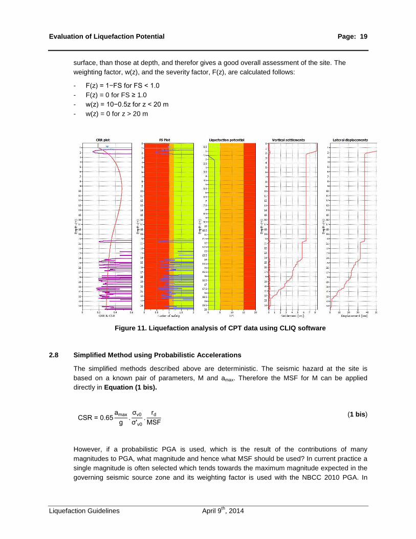
A sample output is given in Figure 11. The distribution of CRR and seismic demand is in the first
cell, followed by distribution of the factor of safety with depth in the second cell. The third cell
shows the distribution of the liquefaction potential index. The last two cells show the vertical
distributions of lateral displacements and settlements.
The Liquefaction Potential Index, LPI, is defined as
L ∫ ( ).w( )d
0
0
(6)
where z is depth of the midpoint of the sublayer under consideration (0 to 20 m) and dz is an
increment in depth. The liquefaction potential gives greater weight to layers which liquefy near the
Evaluation of Liquefaction Potential Page: 19
Liquefaction Guidelines April 9th, 2014
surface, than those at depth, and therefor gives a good overall assessment of the site. The
weighting factor, w(z), and the severity factor, F(z), are calculated follows:
- 1− S for S 1.0
- F(z) = 0 for FS 1.0
- w 10−0. for 0 m
- w(z) = 0 for z > 20 m
Figure 11. Liquefaction analysis of CPT data using CLIQ software
2.8 Simplified Method using Probabilistic Accelerations
The simplified methods described above are deterministic. The seismic hazard at the site is
based on a known pair of parameters, M and amax. Therefore the MSF for M can be applied
directly in Equation (1 bis).
CS 0.6 amax
g. 0
0.
rd
S
(1 bis)
However, if a probabilistic PGA is used, which is the result of the contributions of many
magnitudes to PGA, what magnitude and hence what MSF should be used? In current practice a
single magnitude is often selected which tends towards the maximum magnitude expected in the
governing seismic source zone and its weighting factor is used with the NBCC 2010 PGA. In

Evaluation of Liquefaction Potential Page: 20
Liquefaction Guidelines April 9th, 2014
Vancouver prior to 2007 M=7.3 was recommended for use. In 2007 M=7.0 was suggested. .Does
these suggested magnitudes represent adequately the combined effects of the many different
magnitudes contributing to the probabilistic PGA? The answer to this question is not a matter of
opinion but can be demonstrated directly by two independent methods: (1) a probabilistic seismic
hazard analysis using weighted magnitudes and (2) a procedure based on a magnitude - distance
deaggregation for the BC code hazard level of a 2% exceedance rate in 50 years. The weighted
magnitude probabilistic analysis approach is described in detail by Finn & Wightman (2007). It
requires access to a seismic hazard analysis program. The deaggregation method is easy to
implement because the magnitude – distance deaggregation is available from USGS. Finn &
Wightman (2007) have shown that both methods give the same results.
2.9 Weighted Residual Method
The weighted magnitude probabilistic analysis approach was first proposed by Idriss (1985). He
demonstrated the need for weighting the magnitudes and showed how for the same acceleration
level the return period for the weighted response could be much longer depending on the seismic
environment. The weighting factors, MWF, used in the study by Idriss are the inverse of the MSF
proposed by Youd et al. (2001).
The weighted magnitude probabilistic analysis is accepted in California as a procedure for
implementing the requirements of the Division of Mines and Geology guidelines in DMG SP 117
and the Seismic Mapping Act for projects requiring review under the Seismic Mapping Act of
California. D G S 11 states “The alternati e approach calculating “magnitude-weighted
accelerations” is considerably easier and it pro ides a unique magnitude to be used with the
probabilistically deri ed accelerations” SCEC 1 .
The weighted magnitude probabilistic analyses reported in this paper were conducted to obtain
the magnitude–acceleration pair for evaluating liquefaction potential. In this context, the weighted
hazard curves are called liquefaction hazard curves. The seismic hazard curve for Vancouver and
the corresponding liquefaction hazard curve weighted for magnitude M = 7.5 are shown in Figure
12.
The acceleration for assessing liquefaction potential for an exceedance rate of 2% in 50 years is
0.30g for M=7.5 and the site factor C=1.0. For other values of C, the compatible acceleration is
0.30g. The liquefaction hazard acceleration should be used directly with the liquefaction
resistance curve for magnitude M=7.5 without further scaling. As pointed out by Idriss (1985) the
weighted probabilistic analysis can be done for any normalizing earthquake magnitude other than
M=7.5 but the appropriate magnitude weighting factor for the chosen normalizing magnitude must
be applied again, when calculating liquefaction resistance using Figure 2. Therefore, when
evaluating liquefaction triggering only, the magnitude-acceleration pair to be used is the
normalizing magnitude and the associated weighted acceleration.

Evaluation of Liquefaction Potential Page: 21
Liquefaction Guidelines April 9th, 2014
Figure 12. Liquefaction and acceleration curves for Vancouver normalized for M = 7.5
The unweighted and weighted PGA are for firm ground and, depending on the intensity of
shaking, will be amplified or deamplified at the surface by a site factor C on propagating through
the softer soils often associated with liquefaction. The site factor C is usually determined by an
appropriate site response analysis. Other options that are used are generalized amplification data
such as provided in Idriss (1990), or the short period amplification factors in NBCC 2005. The
factors of safety against liquefaction presented in the following were calculated by the simplified
method for a range in (N1)60 values using the magnitude-acceleration pair from the weighted
magnitude probabilistic analysis. Generic site conditions were assumed, consisting of sand, with
unit weight 20 kN/m3, a water table at 2m, and a range of (N1)60 values at 6m depth. For these
analyses the site factor was assumed to be C=1. The factors of safety are shown in Table 8.
Current practice in Vancouver for evaluating liquefaction potential is to use the NBCC 2005
accelerations with a magnitude M = 7.3. The factors of safety from this approach are also given in
Table 8.

Evaluation of Liquefaction Potential Page: 22
Liquefaction Guidelines April 9th, 2014
Table 8. Factors of safety against liquefaction for Vancouver
SPT Blowcount, (N1)60 Liquefaction Triggering Safety Factors for Vancouver
Current Practice Weighted Magnitude Analysis
M7.3:0.46g M7.5:0.30g
10 0.28 0.40
13 0.35 0.49
15 0.39 0.57
18 0.47 0.67
20 0.53 0.76
25 0.72 1.02
30 1.15 1.64
O er the range 10 1)60 0, the factors of safety from the weighted magnitude probabilistic
analysis are about 43% greater than the factors given by current practice in Vancouver. If the
magnitudes are weighted relative to M = 7.3, the recommended magnitude for Vancouver, the
weighted magnitude probabilistic analysis gives a liquefaction acceleration of 0.35g. When M
=7.3 (with MSF = 1.07) and amax =0.35g are used in the simplified liquefaction assessment
procedure, the factors of safety are similar to those shown for M = 7.5 and amax =0.30g in Table 8.
2.10 Magnitude Deaggregation Method
The magnitude deaggregation method will be explained with reference to the magnitude-distance
deaggregation for Vancouver shown in Figure 13 (Halchuk & Adams 2006). In this case the
magnitudes are collected in bins 0.25M wide and the central magnitude value is assigned to the
bin. For example the bin labeled M=5.125 contains all earthquakes in the range 5.0 M < 5.25.
The contributions of the bin magnitude to the site acceleration are sampled at various distances
from the site. These contributions are shown by the row numbers in the magnitude contribution
matrix in Figure 14.
The contributions are given per mil (1000) for convenience and are divided by 10 to give the
percent contribution. The total contributions per magnitude bin are obtained by summing the
distance contributions horizontally. The cumulative per cent contributions per magnitude bin are
shown in the 2-D plot in Figure 15. The sum of the bin contributions is 100%.

Evaluation of Liquefaction Potential Page: 23
Liquefaction Guidelines April 9th, 2014
Figure 13. Magnitude-distance deaggregation for NBCC 2005 PGA in Vancouver
Figure 14. Deaggregation matrix for NBCC 2005 PGA in Vancouver
Figure 15. Magnitude Contributions to NBCC 2005 PGA Hazard in Vancouver
The factor of safety against liquefaction at a site, taking into account the magnitude scaling
factors is calculated as follows. The factor of safety of the site at the code acceleration level is
computed for each binned magnitude and then multiplied by the contribution of the magnitude to
the site acceleration. The sum of all the contributions to the factor of safety gives the global factor
of safety for the site. The calculation process for Vancouver is shown by the example in Table 9.

Evaluation of Liquefaction Potential Page: 24
Liquefaction Guidelines April 9th, 2014
Table 9. Sample calculation for factor of safety against liquefaction for Vancouver site with (N1)60=18 at 6m depth
Magnitude
Bins
Central
Magnitude
Contribution
Factor
Liquefaction
S.F.
S.F.
Contribution
4.75 – 5.0 4.875 0.033 1.33 0.044
5.0 – 5.25 5.125 0.045 1.17 0.052
5.25 – 5.5 5.375 0.058 1.03 0.060
5.5 – 5.75 5.625 0.074 0.92 0.068
5.75 – 6.0 5.875 0.091 0.82 0.075
6.0 – 6.25 6.125 0.109 0.74 0.080
6.25 – 6.5 6.375 0.126 0.67 0.084
6.5 – 6.75 6.625 0.143 0.60 0.086
6.75 – 7.0 6.875 0.157 0.55 0.086
7.0 – 7.25 7.125 0.163 0.50 0.082
Sum 1.000 Total Factor of Safety = 0.72
The factors of safety from the deaggregation method are compared in Table 10 with the factors
obtained using the magnitude-acceleration pair from the magnitude weighted probabilistic
analysis. The factors given by previous (M=7.3) and current practice (M=7.0) in Vancouver and
those arising from using mean and modal magnitudes with the code acceleration are also shown.
The mean magnitude, deaggregation and weighted magnitude methods give factors of safety
within an average of 2% of each other. The simplest approach seems to be the mean magnitude
combined with the estimated peak ground acceleration for the appropriate hazard level.

Evaluation of Liquefaction Potential Page: 25
Liquefaction Guidelines April 9th, 2014
Table 10. Factors of safety against liquefaction in Vancouver for various triggering options
SPT Blow-
Count (N1)60
Modal
Magnitude
(M7.1: 0.46g)
Current
Practice
(M=7.0)
Mean
Magnitude
(M6.3: 0.46g)
Deaggregation
Method
(M7.25-4.75:
0.46g)
Weighted
Magnitude
Analysis
(M7.5: 0.30g)
10 0.30 0.32 0.40 0.41 0.40
13 0.37 0.39 0.50 0.51 0.49
15 0.42 0.44 0.57 0.58 0.57
18 0.50 0.53 0.68 0.72 0.67
20 0.56 0.59 0.77 0.78 0.76
25 0.76 0.81 1.04 1.05 1.02
30 1.22 1.29 1.66 1.69 1.64
Figure 16. Liquefaction potential for various (N1)60cs values and seismic site conditions,
using Youd et al. (2001)
The analyses were repeated for a peak ground acceleration of 0.35g, which was obtained by site
response analysis. The factors of safety were evaluated by the deaggregation, mean magnitude
and using current practice with M=7.0 and PGA=0.35g. The results are shown in Figure 16.

Evaluation of Liquefaction Potential Page: 26
Liquefaction Guidelines April 9th, 2014
Figure 17. Liquefaction potential for various (N1)60cs values and amax=0.35g, using Youd et
al. (2001)

Consequences of Liquefaction in Terms of Ground Displacements Page: 27
Liquefaction Guidelines April 9th, 2014
3.0 Liquefaction or Cyclic Failure of Fine-Grained Clays and Plastic Silts
3.1 Simplified Stress Analysis for Plastic Soils
The cyclic failure of clays and plastic silts depends on the balance between seismic demand and
resistance capacity. As in the case of sands, the Simplified Procedure by Seed and Idriss (1971)
will be used to estimate the seismic demand in terms of the cyclic stress ratio, CSR given by
Equation (1 bis).
CS 0.6 amax
g. 0
0.
rd
S
(1 bis)
The magnitude scaling factor, MSF, is defined as
S C
C .
(7)
The MSF is used to convert a cyclic stress ratio due to a given magnitude, M, to the equivalent
stress ratio for M=7.5. The cyclic behavior of plastic soils is very different from that of sands and
so the equivalent stress ratios will be different. Boulanger and Idriss (2004) developed MSF for
plastic soils to facilitate the application of the Simplified Method to clays and plastic silts. Their
report presents a careful, fundamental analysis of the cyclic behavior of plastic soils and deserves
detailed study. The MSF for clay is given by
S 1.1 exp w
⁄ 0. (8)
with the S clay 1.1 compared with the S sand 1. .
MSF clay is plotted in Figure 18. The MSF for sand is shown for comparison. The variation of
MSF clay with magnitude is quite flat. Values range from a maximum value of 1.13 at Mw=5.0 to
approximately 1.0 at Mw = 8.5. The corresponding range for sands is 1.18 – 0.8.

Consequences of Liquefaction in Terms of Ground Displacements Page: 28
Liquefaction Guidelines April 9th, 2014
Figure 18. Magnitude scaling factors for converting a cyclic stress ratio due to a
magnitude, M, to the equivalent cyclic stress ratio for M = 7.5 for sand like and clay like
soils (Boulanger and Idriss, 2004)
3.2 Resistance Capacity, CRR
The cyclic resistance ratio, CRR, for cohesionless soils has been established as a function of
normalized quantities: SPT-N, Qc and Vs and therefore can be determined from routine in situ
field measurements. A similar data base is not available for clays. There are 3 recognized
methods for determining CRR for clays (Boulanger and Idriss, 2004):
1. The direct method using cyclic loading tests on high quality samples
2. Measure the monotonic undrained shear strength, Su, in situ or by test on high quality
samples
3. Estimate Su based on the stress history of the soil profile
Method 1.
The proper use of Method 1 requires that state of practice protocols for sampling and testing be
followed.
Method 2.
The vane shear test, VST, provides the best estimate of Su, by in situ methods. It also allows the
determination of residual strength, Sr, and therefore gives a measure of the Sensitivity of the clay:

Consequences of Liquefaction in Terms of Ground Displacements Page: 29
Liquefaction Guidelines April 9th, 2014
S Su
Sr
(9)
The measured Su has to be adjusted to field alue using a correction factor μ Bjerrum, 1
giving:
( u)field μ Su ST (10)
The μ factor is in Figure 19 as a function of PI.
Figure 19. Correction factor μ for ST measurements of undrained strength Ladd and DeGroot
2003, after Ladd et al. 1977)
The undrained strength can be estimated from CPT tip resistance by the relation:
Su qct
(12)
Nk can have a range of 10-30 but for normally consolidated and lightly over-consolidated clays a
value of Nk = 14 is often used.
3.3 Estimating CRR from Su Profile
The CRR when M = 7.5 can be estimated for Su profiles obtained by either Method 1 or 2 using
Equation (13).

Consequences of Liquefaction in Terms of Ground Displacements Page: 30
Liquefaction Guidelines April 9th, 2014
CRRM = 7.5 τcyc/Su)N = 30 (Su/ ivc)
(13)
The cyclic shear stress τcyc is 6 % of the pea shear stress as for sand but the ratio τcyc/Su)N = 30
is evaluated from a substantial data base for N = 30 cycles when M = 7.5. The value 0.83 was
selected for clay-like soils subjected to direct simple shear loading conditions. This value may
change as more data as more data becomes available. For the present, CRR is given by
Equation (14):
CRRclay = 0.83 (Su/ ivc) (14)
If a correction factor C2D = 0.96 is included to represent the fact that motions occur in the field in
two directions then:
CRRclay = 0.8 (Su/ ivc)
(15)
3.4 Method 3
The CRR may also be estimated from the stress history of the soil profile i.e. the consolidation
history. The undrained shear strength may be related to ivc and OCR as follows:
Su/ ivc = S. OCR
m (16)
Then from Equation (15) the CRR is given by:
CRRM = 7.5 = 0.8 S OCRm
(17)
Based on research by Ladd (1991), Boulanger and Idriss (2004) recommended S = 0.22 and m =
0.8 for homogeneous, low to high plasticity, sedimentary clays. Then:
CRRM = 7.5 = 0.18 OCR0.8
(18)
3.5 Effect of Initial Static Shear Stress
As in the case of sand the CRR is affected by the presence of an initial static shear stress when
the site is sloping. n this case the le el ground C must be multiplied by the slope factor .
The . is shown in Figure 20 as a function of the initial static shear stress ratio and the o er-
consolidation ratio OCR.

Consequences of Liquefaction in Terms of Ground Displacements Page: 31
Liquefaction Guidelines April 9th, 2014
Figure 20. The slope correction factor Kα as a function of initial static shear stress ratio
and OCR
3.6 Consequences of Cyclic Failure in Plastic Soils
Unlike the case of sands, there are no empirical formulas to estimate lateral spreading in clay-like
soils. Boulanger and Idriss (2004) and Idriss and Boulanger (2008) suggest using the Newmark
sliding block analysis to estimate deformations on potential sliding surfaces. The shear strength
may be the remolded strength or a strain depend shear strength may be used. The Newmark
method assumes a rigid block sliding on a failure surface. If a significant volume of soils is
involved in the sliding failure the displacement are likely to be underestimated. A nonlinear site
response analysis will give an estimate of the distribution of shear strains in the vertical direction
and provide the basis for estimating lateral spreading,

Consequences of Liquefaction in Terms of Ground Displacements Page: 32
Liquefaction Guidelines April 9th, 2014
4.0 Consequences of Liquefaction in Terms of Ground Displacements
4.1 General
Broadly speaking there are 2 approaches in common use for estimating the amount of lateral
spreading in liquefiable ground for school projects, once the possibility of flow failure is
eliminated. The first class of methods is exemplified by Youd et al. (2002) who assembled a
database of lateral spreading observations and developed regression equations for lateral spread
prediction, based on geotechnical profile information and the magnitude and distance of the
triggering event. The second class of methods uses laboratory data from simple shear testing and
shake table testing to arrive at cyclic strain limits once liquefaction is triggered in materials of
various initial densities (and field penetration resistance). The lateral displacements are the
calculated from the strains. Idriss and Boulanger (2008, pp 133-135) give a very lucid description
of the various shear strain based methods.
4.2 Youd et al. (2002) Model
Bartlett and Youd (1995) compiled a large database of lateral spreading case histories from
Japan and the western United States and developed a regression-based predictive relationship.
Youd et al. (2002) used an expanded and corrected version of the 1992 database to develop the
predictive relationship for displacement. The database is illustrated in Figure 21.
Figure 21. Measured versus predicted displacements for displacements of up to 2m
The displacement for given seismic and site conditions is given by Equation 19.

Consequences of Liquefaction in Terms of Ground Displacements Page: 33
Liquefaction Guidelines April 9th, 2014
log DH = b0 + b1 Mw + b2 log R* + b3 R + b4 log W + b5 log S
+ b6 log T15 + b7 log(100-F15) + b8 log(D5015+0.1 mm)
(19)
where DH = horizontal displacement in meters and R* = R +10−0.89Mw −5.64. The values of the
coefficients are presented in Table 11.
Table 11. Coefficients for Youd et al. (2002) predictive equation
Model
b0 b1 b2 b3 b4 b5 b6 b7 b8
Ground
slope -16.213 1.532 -1.406 -0.012 0 0.338 0.540 3.413 -0.795
Free
face -16.713 1.532 -1.406 -0.012 0.592 0 0.540 3.413 -0.795
The geometric parameters of the site are shown in Figure 22.
Figure 22. Slope geometry notation
Check the applicability of the Youd et al. (2002) model to the site of interest by comparing the
parameters obtained in the preceding steps against the ranges shown in Table 12. The results of
any analyses based on parameters that lie outside these ranges should be interpreted very
carefully.

Consequences of Liquefaction in Terms of Ground Displacements Page: 34
Liquefaction Guidelines April 9th, 2014
Table 12. Range of allowable variable values for use with the Youd et al. (2002) predictive
equation
Variable
Description Range
T15 Equivalent thickness of saturated cohesionless soils (clay
content 1 % in m.
1 to 15m
M Moment magnitude of the earthquake 6.0 to 8.0
ZT Depth to the top of the shallowest layer contributing to T15 1 to 15m
W Free face ratio 1 to 20%
S Ground slope 0.1 to 6%
F15,
D5015
Applicable combinations of F15 and D5015 should be obtained
from the figure below
For given site conditions, the lateral spreading depends on the seismicity parameters M and D.
Youd et al. (2002) provided the chart shown in Figure 23 for obtaining the equivalent distance for
use in Equation 19.

Consequences of Liquefaction in Terms of Ground Displacements Page: 35
Liquefaction Guidelines April 9th, 2014
Figure 23. Graph for determining equivalent source distance, Req, for magnitude, M, and
peak acceleration, amax.
The above curves are the averages of PGA from three different attenuation relations:
Abrahamson and Silva, 1997; Boore et al. 1997; and Campbell, 1997. For the Abrahamson and
Silva, 1997 relation, the following parameters were used in the regression equation: R equals the
distance to the fault rupture, fault type was set to ‘‘otherwise’’, HW5 hanging wall factor was set to
1, which implies that sites are found on the hanging wall, site classification was set to 1 for deep
soil sites. For the Boore, Joyner and Fumal, 1997 relation, the following parameters were used in
the regression equation: R is the closest horizontal distance in km to a vertical projection of fault
rupture surface in km; Vs in the upper 30 of the site was set to 270m/s which is the mid - range for
a medium stiff soil site, Class D, fault type was set to ‘‘fault mechanism not specified.’’ or the
Campbell 1997 relation, the following parameters were used in the regression equation: R is the
closest distance to the seismogenic rupture surface m, fault style factor was set to ‘‘otherwise’’,
soft rock and hard rock site factors were set to ‘‘otherwise’’, which implies a stiff soil site.
4.3 Lateral Displacements using Magnitude-Distance Deaggregation
When dealing with probabilistic ground motions in BC, as pointed out in the Liquefaction Section,
a magnitude M=7.0 is selected and paired with a peak probabilistic ground motion selected from
either, a hazard analysis, or from a site response analysis using input motions which match the
probabilistic design spectrum that has an exceedance rate of 2% in 50 years. This probabilistic
acceleration is made up of the a erage site acceleration plus ε , where is the standard
de iation and ε is the number of standard de iations required to reach the probabilistic alue. For
Vancouver the average ε=1.72. Using such a high acceleration in Figure 23 results in overly
short distances and consequently, inflated estimates of displacement.

Consequences of Liquefaction in Terms of Ground Displacements Page: 36
Liquefaction Guidelines April 9th, 2014
Average acceleration method: The average acceleration at the site may be obtained by running
a ha ard analysis for the site with ε 0. An average acceleration of 0.20g for the Lower Mainland
is appropriate. Using this average acceleration results in significantly longer distances, D, and
correspondingly smaller lateral spreading displacements.
Deaggregation method: The deaggregation method used in evaluating liquefaction potential
may also be used here. For each magnitude-distance pair in the deaggregation matrix, we
compute the corresponding lateral displacements using Youd’s Equation (19). These
displacements are then multiplied by the corresponding probability density given by the
deaggregation for that magnitude-distance pair. This results in a new spreadsheet of lateral
displacement values. The displacements corresponding to any magnitude bin are summed
horizontally and then the sums at the end of each row are summed to give the total horizontal
displacement.
The spreadsheet of displacements calculations used in the deaggregation method in shown in
Figure 24. Cells that show zero values represent infinitely small displacements which are omitted
for clarity. This spreadsheet also shows the clear separation of the contributions of the smaller
and shallower earthquakes compared to the larger subcrustal earthquakes. Notice that influence
of the latter kick in at distances of greater than 50km. The typical deaggregation available on the
GSC Website (nrcan.gc.ca) is not suitable for this calculation because the distance bins are too
large. If requesting a magnitude-distance deaggregation from GSC, specify a distance bin size of
5km.
Figure 24. Sample calculation of lateral spreading displacements using the
deaggregation method
Both of these methods are applied to a school project site in Delta to evaluate the lateral
spreading displacements. The probabilistic PGA from site response analysis was 0.35g. The site
parameters are as follows: average ground slope, S = 0.5%, D5015 = 0.25mm, F15=5% and T15
varies with location at the site. The T15 values for the 6 site locations are 8.60m, 8.80m, 7.75m,
9.95m, 4.95m and 7.95m, respectively. The lateral spreading displacements are calculated using
Youd et al. (2001) following current practice. For M=7.0, a =0.35g, Figure 23 gives an

Consequences of Liquefaction in Terms of Ground Displacements Page: 37
Liquefaction Guidelines April 9th, 2014
approximate distance ≈1 m, Computed displacements using equation 2 are shown is green in
Figure 18. The displacements are also calculated for M=7.0 and an average acceleration of
0.20g, which gives a distance R=25km, and are shown in blue in Figure 25. Finally, the
deaggregation method is also used and the results are shown in red in Figure 25. It `is clear that
using the probabilistic peak ground acceleration to determine the equivalent distance for use in
the Youd equation gives inflated estimates for lateral spreading displacement. it seems
acceptable to estimate displacements on the basis of M=7.0 and an average site acceleration of
0.2g.
As was seen from Figure 25, the displacements computed using the deaggregation method and
the average acceleration method are approximately 50% of the Youd et al. (2001) displacements.
The difference with the Youd displacements is accounted for by the fact that the probabilistic
acceleration, rather than the average acceleration, was used to calculate the displacements.
These differences in displacement have very serious consequences for the retrofit program. If
refined magnitude=distance deaggregation is not available from GSC to allow effective use of the
deaggregation method, it is recommended that future displacements for school projects be
estimated using the Youd et al. procedure with an average acceleration of 0.20g and M=7.0.
Figure 25. Calculated displacements for the school site in Delta
4.4 Idriss and Boulanger (2008) Model
Idriss and Boulanger (2008) and Zhang et al. (2004) present methods for estimating lateral
spreading displacements based on laboratory test data. Idriss and Boulanger (2008) present a
method for estimating the maximum shear strains that may occur in a liquefiable layer during
earthquake shaking. Their procedure is based on shear strains estimated from cyclic laboratory
testing of saturated sands at various densities by Ishihara & Yoshimine (1992). The maximum
shear strains are limited to the bounds proposed by Seed et al. (1985) and shown in Figure 26,
which were computed using Equation (20) (Idriss and Boulanger 2008).

Consequences of Liquefaction in Terms of Ground Displacements Page: 38
Liquefaction Guidelines April 9th, 2014
lim 1. (1.1 √
1 60,cs
6)
(20)
Figure 26. Limiting shear strains, γl, as a function of (N1)60,cs
The lateral displacement, LD, is computed using Equation (21)
LD ∫ d max
0
(21)
4.5 Zhang et al. (2004) Model
Zhang et al. (2004) made use of a laboratory test-based relationship among “maximum cyclic
shear strain,” relati e density, and factor of safety against liquefaction shihara and Yoshimine,
1992) to develop a cumulative shear strain model for predicting maximum lateral spreading
deformations using Equation (22). He introduced the term Lateral Displacement Index (LDI) to
describe these lateral displacements.
LD ∫ max
d max
0
(22)
Maximum cyclic shear strains were defined by Ishihara and Yoshimine (1992) as the maximum
shear strain (in any direction) under transient loading conditions. Zhang et al. (2004) capped the
maximum cyclic shear strains by the limiting shear strains proposed by Seed (1979) and used
empirical relationships between relative density and penetration resistance (SPT or CPT) to allow
lateral spreading displacement to be predicted. Using the penetration resistance and factor of

Consequences of Liquefaction in Terms of Ground Displacements Page: 39
Liquefaction Guidelines April 9th, 2014
safety against liquefaction (Figure 27) to determine the maximum shear strain, max. Zhang et al.
(2004) recommend the use of a modified form of eyerhof’s relationship to estimate relati e
density as
Dr 16√ 1 1 √ 1 60 for (N1)60 < 42.
(23)
Figure 27. Variation of maximum cyclic shear strain with factor of safety and relative
density (after Zhang et al., 2004)
Zhang et al. (2004) modified the LDI on the basis of field data of observed lateral displacements.
The modified equations are given in Equation (24) for displacements due to sloping ground and
a free face.
D {(S 0. )LD , ground slope case
6 0.
LD , free face case
(24)
The lateral displacements calculated by Youd et al. (2002), Idriss and Boulanger (2008) and
Zhang et al. (2004) for a school site in Delta are shown in Figure 28. It is clear that Idriss and
Boulanger (2008) seriously overestimate the displacements. This results from the fact that the
displacement estimates are based entirely on shear strains without correlation with field data. As
shown in Figure 25, displacements calculated by the average acceleration or the deaggregation

Consequences of Liquefaction in Terms of Ground Displacements Page: 40
Liquefaction Guidelines April 9th, 2014
method are approximately 50% of those calculated by Youd et al. (2001). These differences in
displacement estimates can have a very significant impact on the potential performance of a
school on this site. It is recommended that lateral spreading be estimated using both the average
acceleration and the deaggregation methods.
Figure 28. Lateral spreading displacements for school site in Delta using three
different methods (Figure courtesy of John Carter, GeoPacific Ltd.)
4.6 Vertical Settlements due to Consolidation after Liquefaction
4.6.1 Ishihara & Yoshimine (1992) Model
The Ishihara & Yoshimine (1992) used the factor of safety against liquefaction, FSL, and various
indicators of soil density (relative density, SPT resistance, and CPT resistance) to predict
volumetric strain. The graphical relationship (Figure 29) shows that volumetric strains increase
when the factor of safety drops below 1.0 – sharply for looser sands and gradually for denser
ones. The Japanese SPT value, N1, used in Figure 29, however, is based on an energy ratio of
72% (i.e., (N1 = 0.833(N1)60).
The volumetric strain strains developed from Figure 29 are based on the factor of safety against
liquefaction. These factors should be based on either the deaggregation method described in the
liquefaction section (preferred) or use the mean magnitude with the probabilistic ground motions
otherwise the settlements will be overestimated.
Idriss and Boulanger (2008, pp152-158) present a very useful discussion on strain based
methods for settlement calculations. Ishihara & Yoshimine (1992) procedure is recommended
here for the present. More detailed study of settlement calculations will be conducted when the
new motions for NBCC 2015 become available and will be reflected in the revised guidelines.

Consequences of Liquefaction in Terms of Ground Displacements Page: 41
Liquefaction Guidelines April 9th, 2014
Figure 29. Variation of volumetric strain with relative density, SPT and CPT resistance, and
factor of safety against liquefaction (after Ishihara & Yoshimine, 1992).
Using the curves in Figure 29 and FSL and density parameters, determine the corresponding
values of volumetric strain. The expected settlement, ΔH, is obtained as the sum of all sublayer
settlements, which are approximated assuming constant volumetric strain within each sublayer.
∑ tiε ,i
n
i 1
(25)
where n is the number of sublayers and li is the thickness of the ith layer.

Structural Considerations Page: 42
Liquefaction Guidelines April 9th, 2014
5.0 Structural Considerations
5.1 General
The evaluation of the effects of liquefaction on a structure is based on the following, for the
purposes of these Guidelines:
During strong shaking, the soil has not liquefied and the demand is as for a Class D/E site
with no degradation of the soil strength or stiffness; the typical assessment or retrofit design
as outlined in the remainder of the Volumes applies. The block must be assessed or
retrofitted as if liquefaction is not an issue.
After strong shaking, on a liquefiable site, the soil liquefies and induces new and different
demands on the structure. The block must be assessed or retrofitted to accommodate these
demands, starting in a partially damaged state as per 5.2.4.
The above two effects are not concurrent
The structure must be assessed and retrofitted to accommodate both effects
If the soil will be improved to eliminate the potential for liquefaction, then the demands have
to be re-assessed for strong shaking effects only, based on the new site Class after the soil
improvement
The structural assessment regarding liquefaction is outlined in this Section and retrofit
considerations are outlined in Section 6 of this Volume.
Effective communication between the structural engineer and the geotechnical engineer is
essential in the assessment of the demands of liquefaction and its influence on the structural
response, and to obtain appropriate geotechnical parameters in order to carry out a retrofit
design.
5.2 Assessment
5.2.1 Existing Information
The following information is essential in the assessment:
Proper foundation drawings, and drawings of the ground floor slab
Reasonable investigation to confirm the extent and depth of foundations as shown on the
drawings (or to determine such information where adequate drawings do not exist)
Determine the bearing pressure on all foundations, due to all self-weight (including additional
dead loads as per NBCC 2010) and 25% of snow load plus 100% of storage loads and a Live
Load allowance (LLa) of 1 kPa; C:DL+ADL+25%SL+100+ Storage+LLa.
Adjacent blocks or structures and their surcharge loads on the foundation of the block being
assessed; proximity effects for punching shear check.

Structural Considerations Page: 43
Liquefaction Guidelines April 9th, 2014
Fully understand the location of the LDRS, VLS, OP walls, and their drift limits.
Knowledge of fundamental soil parameters such as, punching shear capacity of non-
liquefiable soil layer, friction coefficient between soil and footings and between soil layers,
passive pressures, modulus of subgrade reaction, down drag effects (if any) on piles, existing
pile capacities, pile depths and expected behavior (friction or end bearing).
5.2.2 Foundations located in Non Liquefiable Crust
Most foundations will be located in a non-liquefiable crust, located over a liquefiable layer, as
illustrated in (a), (b), (e) in Figure 30 below (or located over a zone of a combination of liquefiable
and non-liquefiable layers).
During liquefaction it is to be assumed that the liquefiable layer offers near-zero vertical
resistance and the only soil resistance vertically is the soil between the underside of the
foundation and the liquefiable layer.
The potential for punching shear failure of the foundations through the crust exists, and must be
assessed.
Figure 30. Foundations located in Crust or in Liquefiable Soil
The punching shear capacity of the soil (for individual pad footings or strip footings) as obtained
from the geotechnical engineer shall be checked versus the calculated bearing pressure on the
underside of the foundation for: all structural loads above grade, all structural related loads below
grade, soil/slab above the footing outline.
a) Footing, no piles
b) Footing on piles that end within the liquefiable soil, assuming no vertical resistance from the
piles; add weight of piles to structural loads to determine bearing pressure

Structural Considerations Page: 44
Liquefaction Guidelines April 9th, 2014
In the case where the piles of a piled foundation extend through the liquefiable layer(s) to a firm
non liquefiable strata, per (e) in the Figure above, the pile capacity shall be checked for the same
loads as condition (a) above, plus the down drag on the pile (if any) of the liquefiable soil to be
provided by the geotechnical engineer. Furthermore, the axial shortening of the pile and
deflection of the pile tip in the lower strata shall be calculated by the geotechnical engineer and
added to the differential vertical settlement discussed in 5.2.6 below, as applicable.
5.2.3 Foundations in liquefiable soil
Should the footings illustrated in condition (c) and (d) in the Figure above be fully founded in the
liquefiable layer, no further assessment is required: remediation such as micropiles, soil
densification, etc. is required.
5.2.4 Allowable structure drifts due to Liquefaction Effects
Due to the strong shaking prior to liquefaction, the residual drift in the structure (due to inelastic
response, some damage) shall be assumed to be 20% of the DDL of the LDRS in each principal
direction of the block (where the peak transient drift during strong shaking is 100% of the DDL).
The maximum allowable drift due to liquefaction effects shall be the Maximum DDL of the LDRS
as outlined in Table 4.1, Part B, Volume 2, or the Design Drift Limit for VLS as outlined in Table
8.1, Part B, Volume 2, whichever is less.
With regards to the LDRS, the Maximum DDL is allowable, regardless of what DDL was used to
accommodate the strong shaking effects.
Liquefaction Drift Limit (LDL) shall accommodate the following three components:
Residual Drift (RD)
Effective Drift demand due to lateral soil (horizontal) spreading effects (EDH)
Effective Drift demand due to differential vertical soil settlement effects (EDV)
Thus RD + EDH + EDV < LDL
For example:
DDL 1% (less than Max DDL for reasons such as toolbox)
Residual Drift @ 20% of DDL 0.2%
Max DDL 2.25% (such as prototype M-3)
VLS limit 4% (such as steel)
LDL 2.25%, lesser of the two governs
EDH 1.5% (see 4.2.(5) below regarding how to determine EDH
EDV 0.8% (see 4.2.(6) below regarding how to determine EDV
Therefore, 0.2% + 1.5% + 0.8% = 2.5% which is greater than the 2.25% LDL; therefore
remediation is required.

Structural Considerations Page: 45
Liquefaction Guidelines April 9th, 2014
5.2.5 Lateral soil spreading effects
The lateral soil spreading effect, H, due to liquefaction shall be determined on all sides of a
block, as shown in Figure 31 below.
Figure 31. Lateral soil spreading effects on all sides of block
or the purposes of assessment, it is assumed that the crust can ‘rupture’ and cause a mo ement
of between any non-interconnected foundations, or bay lines, or VLS or line of LDRS in the
block and shall be provided by the geotechnical engineer. This “rupture” is illustrated in Figure
32; between two lines of footings on (a) and (b) in the section, and between any line of footings in
the plan view.

Structural Considerations Page: 46
Liquefaction Guidelines April 9th, 2014
Figure 32. Lateral soil spreading effects
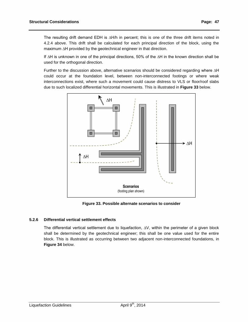
Structural Considerations Page: 47
Liquefaction Guidelines April 9th, 2014
The resulting drift demand ED is /h in percent; this is one of the three drift items noted in
4.2.4 above. This drift shall be calculated for each principal direction of the block, using the
maximum pro ided by the geotechnical engineer in that direction.
f is un nown in one of the principal directions, 0% of the in the nown direction shall be
used for the orthogonal direction.
Further to the discussion above, alternative scenarios should be considered regarding where
could occur at the foundation level, between non-interconnected footings or where weak
interconnections exist, where such a movement could cause distress to VLS or floor/roof slabs
due to such localized differential horizontal movements. This is illustrated in Figure 33 below.
Figure 33. Possible alternate scenarios to consider
5.2.6 Differential vertical settlement effects
The differential ertical settlement due to liquefaction, , within the perimeter of a gi en bloc
shall be determined by the geotechnical engineer; this shall be one value used for the entire
block. This is illustrated as occurring between two adjacent non-interconnected foundations, in
Figure 34 below.

Structural Considerations Page: 48
Liquefaction Guidelines April 9th, 2014
Figure 34. Differential Vertical Settlement Effects
For the purposes of assessment, it is assumed that the crust can ‘shear’ to accommodate the
une en settlements in the liquefiable soil layer and cause a mo ement of between any
foundations non-interconnected or connected by an element without adequate capacity to
accommodate the differential settlement, or baylines, or VLS or line of LDRS in the block.
The resulting effecti e drift demand ED is /L1 as shown in Figure 34), or it can be /L or
/L in the other spans shown, in percent. These effecti e drifts shall be calculated for each
principal direction of the block, using the maximum effective drift demand in a given direction.
This calculated drift EDV is one of the three drift terms noted in 5.2.4.
5.2.7 Connections
Connections affected by rotation and/or lateral loads shall be checked to ensure the new
demands on the connections cannot cause local or global collapse.
Figure 32 illustrates discrete or integral connections that shall be checked for:
Any additional tension loads induced in the diaphragm due the lateral spreading effects
Any potential movement of the diaphragm, should the tension load induce local connection
failure, and allow movement of the diaphragm (and its beams) relative to the local support of the
diaphragm
All affected connections shall be investigated.

Remedial Options Page: 49
Liquefaction Guidelines April 9th, 2014
6.0 Remedial Options
6.1 General
Any remedial work required is based on providing life safety and prevention of collapse, so that
an affected facility can be safely evacuated in the event of a major earthquake. Structures may or
may not be re-usable after the event.
The options for mitigation of liquefaction and its consequences for an existing building will
generally fall into two categories: soil remediation, or structural modifications.
6.2 Soil Remediation
There are a wide variety of techniques for soil remediation that can be used to mitigate the effects
of liquefaction or excessive cyclic softening, such as:
in-situ densification using vibro-replacement or vibro-compaction or dynamic compaction,
in-situ strength and stiffening using compaction grouting, jet grouting, deep soil mixing,
shallow soil mixing.
excavate and replace with compacted engineered fill.
load transfer to non-liquefiable materials using piling.
All of these techniques are disruptive for an existing facility and usually quite expensive, so that
preferred methods very often are structural, whereby a building is retrofit to provide it with the
ability to withstand large deflections either laterally or vertically or both, to a sufficient degree that
allows safe egress for its occupants.
One possible exception to the foregoing is in the case where there is a significant lateral
spreading hazard to the building by virtue of an adverse ground slope or proximity to a river bank
or similar free face towards which the lateral spreading will migrate. In such a case the amount of
lateral spread movement can sometimes be limited by the installation of a so-called “seismic
di e”. This is a zone of ground improvement of the liquefiable material of dimensions sufficient to
provide resistance to lateral spreading and post-earthquake stability. This can be achieved with a
variety of in-situ soil improvement techniques. See the Vancouver Task Force (2007) report for
more discussion of methods and design philosophy and references thereto. Of course a retrofit
using a perimeter seismic dike can only provide a level of protection against lateral
displacements, and vertical post-earthquake settlements and/or punching failure of shallow
foundations remain to be dealt with structurally.
Idriss and Boulanger (2008, pp 167-183) present a very useful review of mitigation measures.
Experience with school projects with liquefaction problems suggests that the first attempt at
mitigation should be structural. Geotechnical mitigation efforts are usually more expensive. In
addition to the direct cost of geotechnical mitigation, the process often requires finding alternative
accommodation for the students – a major expense.

Remedial Options Page: 50
Liquefaction Guidelines April 9th, 2014
6.3 Structural Remediation
There are a wide variety of techniques for structural remediation that can be used to mitigate the
effects of liquefaction, if there are deficiencies in the structure and foundation based on the
assessment in Section 4.
6.3.1 For inadequate punching shear capacity
(a) enlarging footings based on punching shear capacity provided by the geotechnical
engineer
(b) adding mini-piles between existing footings, with a new grade beam connected to existing
footing; the minipiles and the new grade beams to be designed to resist 100% of the
loads unless it can be shown otherwise
(c) creating a complete raft foundation, interconnecting all existing footings; geotechnical
engineer to provide modulus of subgrade reaction for raft footing design
6.3.2 For excessive lateral spread effects
(a) Interconnect all footings inside the building, with new tension ties.
(b) Create an external ring beam (fully or partially around perimeter as required) to minimize
differential movement between footings.
The compression struts or slab on grade within the building perimeter to be designed to
resist all sliding forces applied to them.
(c) Creating a complete raft foundation, interconnecting all existing footings.
(d) LDRS that has larger maximum DDL (to increase drift limit).
(e) Supplementary supports at adversely affected VLS (to increase drift limit).
(f) Modify VLS to accommodate larger drift limits; for example, if short columns created by
partial height infills limit the DDL, add deflection gaps to eliminate the short column effect
and increase the DDL of the system.
6.3.3 For excessive differential vertical settlements
Similar to 1 (b) noted above
Similar to 2 (c), (d) and (e) noted above
6.4 Enhanced Performance Retrofit
For blocks with an objective of Enhanced Performance Retrofit the concept of distortion damage
should be considered and evaluated. The relationship between angular distortion ß and lateral
strain ƐL to be ept below the “Se ere to ery se ere damage” area as shown in Figure 35
below.

Remedial Options Page: 51
Liquefaction Guidelines April 9th, 2014
Figure 35. Damage Criteria consideration for Enhanced Performance Retrofit
For further information, refer to Boscardin and Cording (1989).

Closing the Loop: Reconciling Geotechnical Demands with Performance Criteria Page: 52
Liquefaction Guidelines April 9th, 2014
7.0 Closing the Loop: Reconciling Geotechnical Demands with Performance Criteria
The following example comes from a seismic retrofit study for a school in Vancouver. Atypical
block is shown in Figure 36. The structural engineer responsible for the retrofit is John
Sherstobitoff, Ausenco Ltd., Vancouver. The performance criteria set out in Section 7.1 are taken
from the Seismic Retrofit Design Guidelines for Schools, 2nd
Edition, 2013.
Figure 36. Cross-section of school building block
7.1 Performance Limits for School
Building Description
– One storey mixed concrete and steel framed structure
– LDRS Concentric braced frame
(Tension-Compression moderately ductile)
• DDL: 2.5%
– VLS Exterior: Non-ductile concrete columns
• DDL: 1.25%
– VLS Interior/Exterior: Steel columns
• DDL: 4%
– Liquefaction Drift Limit
• LDL: 4% or 2.5% * lesser of the two
• * if liquefaction effects can cause such deformation

Closing the Loop: Reconciling Geotechnical Demands with Performance Criteria Page: 53
Liquefaction Guidelines April 9th, 2014
7.2 Estimation of Total Drift
Drift Components to be considered are
– Residual drift (RD) from seismic excitation
– Effective drift demand due to lateral soil spreading (EDH)
– Effective drift demand due to vertical soil settlement (EDV)
– RD + EDH + EDV < LDL
These are illustrated in Figure 37. EDV is not a drift. A pseudo drift is computed using the
settlement Δ . This is added to the other drifts to give a conservative estimate of total drift
demand.
Figure 37. Summing up the displacement from different sources
7.3 Geotechnical Engineer Input
Geotechnical Engineer to provide
– Differential free field vertical movement
– Differential free field horizontal movement
– Friction coefficient between soil and foundations
– Bearing capacity on crust
– Soil pressure on grade beams
– Based on vertical loads at each foundation provided by the Structural Engineer, the
Geotechnical Engineer will determine if there is risk of punching for each foundation
– Differential movement is too large, since the existing foundations are not
adequately tied together in two directions

Closing the Loop: Reconciling Geotechnical Demands with Performance Criteria Page: 54
Liquefaction Guidelines April 9th, 2014
Figure 38. Effect of tying foundations together with grade beams.
Figure 39. Building in Christchurch underwent rotation but no relative displacement
across the base during the Canterbury earthquake.

Closing the Loop: Reconciling Geotechnical Demands with Performance Criteria Page: 55
Liquefaction Guidelines April 9th, 2014
Figure 40. Plan of Building
7.4 Retrofit Details
Total drift due to liquefaction: 3.86 %. The designer decided to add two exterior steel columns at
each side of the existing concrete columns to minimize the impact to the inside of the building,
The new steel columns were designed to carry all the loads carried by the existing concrete
columns. This retrofit option allowed an increase in the DDL of the VLS to 4% which can
accommodate the liquefaction driven drift of 3.86% to be accommodated.
Figure 41. Plan of Building

Closing the Loop: Reconciling Geotechnical Demands with Performance Criteria Page: 56
Liquefaction Guidelines April 9th, 2014
7.5 Finished Project
Figure 42. Finished Project

References Page: 57
Liquefaction Guidelines April 9th, 2014
8.0 References
Andrus, R.D., Stokoe, K.H., Chung, R.M., and Juang, C.H. (2003). Guidelines for Evaluating Liquefaction Resistance Using Shear Wave Velocity Measurements and Simplified Procedures. NIST GCR 03-854, National Institute of Standards and Technology, Gaithersburg, MD, USA. Andrus, R.D. and Youd, T.L. (1987). Subsurface Investigation of a Liquefaction-Induced Lateral Spread, Thousand Springs Valley, Idaho. US Army Corps of Engineers, Miscellaneous Paper GL-87-88. Andrus, R.D. and Stokoe, K.H. (2000). Liquefaction resistance of soils from shear-wave velocity. ASCE Journal of Geotechnical and Geoenvironmental Engineering, 126(11): 1015-1025. Bartlett, S.F. and Youd, T.L. (1995). Empirical prediction of liquefaction-induced lateral spread. ASCE Journal of Geotechnical Engineering, 121(4): 316-329. Bjerrum, L. (1972). Embankments on soft ground. In: Proceedings of the ASCE Conference on Performance of Earth-Supported Structures, Purdue University, 2, 1-54. Boscardin, M.D. and Cording, E.J. (1989). Building Response to Excavation-Induced Settlement. ASCE Journal of Geotechnical Engineering, 115(1): 1-21. Boulanger, R.W. and Idriss, I.M. (2004). Evaluating the Potential for Liquefaction or Cyclic Failure of Silts and Clays, Report No. UCD/CGM-04/01, Center for Geotechnical Modeling, Department of Civil and Environmental Engineering, University of California, Davis, USA. Boulanger, R.W. and Idriss, I.M. (2014). Reply to discussion of CPT-Based Liquefaction Triggering Procedure. To appear in ASCE Journal of Geotechnical and Geoenvironmental Engineering, 2014. Cetin, K., Seed, R., Der Kiureghian, A., Tokimatsu, K., Harder, L., Jr., Kayen, R., and Moss, R. (2004). Standard Penetration Test-Based Probabilistic and Deterministic Assessment of Seismic Soil Liquefaction Potential. ASCE Journal of Geotechnical and Geoenvironmental Engineering, 130(12): 1314-1340.
DeGroot, D.J. and Ladd, C.C. (2012). Site Characterization for Cohesive Soil Deposits Using Combined In Situ and Laboratory Testing. Geo-Congress 2012 SOP Lecture, ASCE Geotechnical Special Publication No. 226. Dobry, R. and Abdoun, T. (2011). An investigation into why liquefaction charts work: A necessary step towards integrating the states of art and practice. Ishihara Lecture, 5
th International
Conference on Earthquake Geotechnical Engineering, Santiago, Chile. Finn, W.D.L. and Wightman, A. (2007). Logical Evaluation of Liquefaction Potential using NBCC 2005 Probabilistic Accelerations. In: Proceedings, Ninth Canadian Conference on Earthquake Engineering, Ottawa, Ontario, Canada, 1894-1993.
Halchuk, S. and Adams, J. (2006). Updated deaggregation of seismic hazard for selected Canadian cities, Personal communication to the authors in advance of publication, Geological Survey of Canada, Ottawa, Canada.
Idriss, I.M. (1985). Evaluating seismic risk in engineering practice. In: Proceedings of the 11
th
International Conference on Soil Mechanics and Foundation Engineering, Vol 1, 255-320.

References Page: 58
Liquefaction Guidelines April 9th, 2014
Idriss, I.M. (1990). Response of soft soil sites during earthquakes. In: Duncan, M. (Ed.) Proceedings H.B. Seed Memorial Symposium, BiTech Publishers Ltd., Vancouver, BC, Canada. Vol.2, 273-290. Idriss, I.M. and Boulanger, R. (2008). Soil liquefaction during earthquakes. MNO-12, Earthquake Engineering Research Institute, Oakland, California.
Ishihara, K. and Yoshimine, M. (1992). Evaluation of settlements in sand deposits following liquefaction During earthquakes. Soils and Foundations, 32(1): 173-188. Ladd, C.C., Foott, R., Ishihara, K., Schlosser, F., and Poulos, H. G. (1977). Stress-deformation and strength characteristics: SOA Report, In: Proceedings, 9
th International Conference on Soil
Mechanics and Foundation Engineering, Vol. 2, 421–494. Ladd, C.C. and DeGroot, D.J. (2003). Recommended practice for soft ground site characterization: Arthur Casagrande Lecture. In: Culligan, P.J., Einstein, H.H. and Whittle, A.J. (Eds.). Proceedings Soil and Rock America, Vol. 1, Verlag Gluckauf GMBH, Essen, Germany. Robertson, P.K. and Cabal (Robertson), K.L. (2010). Guide to Cone Penetration Testing for Geotechnical Engineering, 4
th Edition. Gregg Drilling and Testing Incorporated, Signal Hill,
California, USA. SCEC, (1999). Recommended procedures for implementation of DMG special publication 117, Guidelines for analyzing and mitigating liquefaction hazards in California, SCEC contribution number 462, Southern California Earthquake Center, University of southern California, CA, 1-63. Seed, H.B. and Idriss, I.M. (1971). Simplified Procedure for Evaluating Soil Liquefaction Potential, ASCE Journal of Soil Mechanics and Foundations, 97(SM9): 1249–1273. Seed, H.B. (1979). Soil liquefaction and cyclic mobility evaluation for level ground during earthquakes. ASCE Journal of Geotechnical Engineering, 105(GT2): 201-255. Seed, H.B., Tokimatsu, K., Harder, L.F. Jr. and Chung, R. (1985). Influence of SPT procedures in soil liquefaction resistance evaluations, ASCE Journal of Geotechnical Engineering, 111(12): 1425-1445. Vallee, R.P. and Skyrness, R.S. (1980). Sampling and In-Situ Density of a Saturated Gravel Deposit. Geotechnical Testing Journal, 2(3): 136-142. Task Force Report (2007). Geotechnical Design Guidelines for Buildings on Liquefiable Sites in Accordance with NBC 2005 for Greater Vancouver Region. Anderson, D.L. and Byrne, P.M. Co-Chairs. Youd, T., Idriss, I., Andrus, R., Arango, I., Castro, G., Christian, J., Dobry, R., Finn, W.D.L., Harder, L., Jr., Hynes, M., Ishihara, K., Koester, J., Liao, S., Marcuson, W., III, Martin, G., Mitchell, J., Moriwaki, Y., Power, M., Robertson, P., Seed, R., and Stokoe, K.H. (2001). Liquefaction Resistance of Soils: Summary Report from the 1996 NCEER and 1998 NCEER/NSF Workshops on Evaluation of Liquefaction Resistance of Soils. ASCE Journal of Geotechnical and Geoenvironmental Engineering, 127(10): 817–833. Youd, T.L., Hansen, C.M. and Bartlett, S.F. (2002). Revised multilinear regression equations for prediction of lateral spread displacement. ASCE Journal of Geotechnical and Geoenvironmental Engineering, 128(12): 1007-1017.

References Page: 59
Liquefaction Guidelines April 9th, 2014
Zhang, G., Robertson, P.K. and Brachman, R.W.I. (2004). Estimating liquefaction-induced lateral displacements using the standard penetration test or cone penetration test. ASCE Journal of Geotechnical and Geoenvironmental Engineering, 130(8): 861-871.