ESTIMATION OF A SEMIPARAMETRIC

IGARCH(1,1) MODEL∗

Woocheol Kim† (Korea Institute of Public Finance)

Oliver Linton‡

(London School of Economics and Universidad Carlos III de Madrid)

The Suntory Centre Suntory and Toyota International Centres for Economics and Related Disciplines London School of Economics and Political Science

DP No: EM 2009 539 Houghton Street October 2009 London WC2A 2AE Tel: 020 7955 6674

∗ We would like to thank Xiaohong Chen, Joel Horowitz, and Eric Renault for interesting discussions. We thank also Jean-Pierre Florens and two referees for helpful comments. † Korea Institute of Public Finance, 79-6 Garak-Dong, Songpa-Gu, Seoul, Republic of Korea, 138-774; email: wkim@kipf.re.kr ‡ Department of Economics, London School of Economics, Houghton Street, London WC2A 2AE, United Kingdom. E-mail address: o.linton@lse.ac.uk. Thanks to the ESRC and Leverhulme foundations for financial support. This paper was partly written while I was a Universidad Carlos III de Madrid-Banco Santander Chair of Excellence, and I thank them for financial support.

Abstract We propose a semiparametric IGARCH model that allows for persistence in variance but also allows for more flexible functional form. We assume that the difference of the squared process is weakly stationary. We propose an estimation strategy based on the nonparametric instrumental variable method. We establish the rate of convergence of our estimator. Key words and phrases: Inverse Problem; Instrumental Variable; IGARCH; Kernel Estimation; Nonparametric regression. Journal of Economic Literature Classification: C14 © The authors. All rights reserved. Short sections of text, not to exceed two paragraphs, may be quoted without explicit permission provided that full credit, including © notice, is given to the source.

1 Introduction

A number of authors have found parameter estimates in GARCH(1,1) models close to the unit root

region, and have proposed using the integrated GARCH or IGARCH process which imposes this

restriction, see for example Engle and Bollerslev (1986). The exponentially weighted moving average

model (EWMA) (aka ‘JP Morgan’ model), which is the special case in which the intercept is set

to zero, is in wide use by practitioners. The IGARCH process although it does not possess a finite

(limiting) variance can be strongly stationary, see Nelson (1990). In fact, IGARCH processes can

also be geometrically strong mixing, see Meitz and Saikonnen (2004).

We propose a semiparametric extension of the IGARCH model. Our model nests the standard

IGARCH(1,1) model, but it allows more flexibility in functional form. It extends the recent model

of Linton and Mammen (2005) to the case where the unconditional variance of the process does

not exist. We propose an estimation method that involves solving a type one integral equation

with estimated operator, Carrasco, Florens and Renault (2006). We establish the rate of uniform

convergence of the nonparametric part of our model and the consistency of the parametric part.

All proofs are given in the appendix.

2 The Model

We suppose throughout that {yt}∞t=−∞ is an observed strongly stationary process. We suppose that

yt = σtεt,

σ2t = βσ2t−1 + (1− β)y2t−1 +m(yt−1), (1)

where εt and ε2t − 1 are martingale difference sequences i.e., E(εt|Ft−1) = 0 and E(ε2t − 1|Ft−1) = 0,

where Ft contains all information upto current period, and m(·) is an unknown function. When

m(y) = ω for some constant ω, the above model reduces to a standard parametric IGARCH(1,1)

model and when ω = 0 it is the EWMA. If m(y) = δy2+ω, then the process is an ‘explosive’ GARCH

process, strictly stationary for some range of δ ≥ 0. In general, we allow the nonparametric function

m(·) to take a flexible form, as long as it satisfies some regularity condition including smoothness, a

nonnegativity constraint (m(·) ≥ 0), and some additional conditions guaranteeing strong stationarity

of yt. The nonparametric term is introduced to correct possible misspecification with a quadratic

growth function of news impact on volatility.

Defining the martingale difference sequence ηt = σ2t [ε2t − 1], we write the squared returns as

1

y2t = σ2t + ηt. By plugging into (1), we get

∆y2t = y2t − y2t−1 = m(yt−1) + (1− β)ηt−1 + ηt − ηt−1

= m(yt−1) + ηt − βηt−1. (2)

The squared returns {y2t } is an integrated process with a functional drift term, m(·), and moving

average error term. If m(·) ≤ c (with c not so large), the model is likely to show a similar dynamics

to the standard IGARCH process.

For our theoretical development, it is important that {∆y2t } satisfies weak stationarity even when

the process {y2t } does not. In the context of linear time series models this is a property that is quite

common, but in the current context it is not obviously possible. Harvey, Ruiz, and Shephard (1994)

say that (in the case where εt is standard normal) “{∆y2t } is stationary and has an ACF like that

of an MA(1) process.” Their argument seems to be based on the fact that the innovation process

ηt appears to be a martingale difference sequence. Although it appears that E[ηt|Ft−1] = 0, this

definition only makes sense if E[|ηt|] < ∞ or limt→∞ E[|ηt||F0] < ∞ [Hall and Heyde (1980)]. In

fact, these conditions do not hold. Therefore, one cannot conclude anything about weak stationarity.

In any case, weak stationarity of ∆y2t requires both its mean and variance to exist, which would

require that limt→∞ E[η2t |F0] < ∞. In fact, {∆y2t } is not weakly stationary in the Gaussian strong

IGARCH. The cause of this counterintuitive (from the point of view of linear processes) behaviour

is due to the i.i.d. innovation. The following example shows that when the innovations are not i.i.d.

one can have {∆y2t } weak stationarity [or at least have finite first moment] even when {yt} is not

weakly stationary.

E������: Consider a semi-strong IGARCH model, i.e., (1) with m(y) = ω and

εt = sign(zt)

{1 +

u2t − 11 + σ2t

}1/2,

where zt, ut are i.i.d. and mutually independent random variables with Esign(zt) = 0 and Eu2t = 1.

It follows that εt and ε2t − 1 are martingale difference sequences and thereby are consistent with (1).

Furthermore, ηt = (u2t −1) (σ2t/(1 + σ2t )) which satisfies E(|ηt|) < ∞, and so we have E(|∆y2t |) < ∞.

However, E (σ2t ) = E (y2t ) =∞. If zt is symmetric about zero, then εt is also symmetrically distributed

both conditionally and unconditionally. Provided ut has finite fourth moment then E([∆y2t ]2) < ∞.

In the sequel we shall assume that the process {∆y2t } is weakly stationary. This has strong and

testable empirical implications and we investigate whether this is a reasonable assumption in some

common datasets below.

An interesting feature of our semiparametric IGARCH model is that the nonlinear correction

term m can be identified independently of β. Significant estimates of m are related directly to

2

misspecification of IGARCH. Also, by means of nonparametric function m, (1) can nest both GARCH

and IGARCH as a special case. This model is related to recent work of Linton and Mammen (2005)

who considered the case with σ2t = βσ2t−1 +m(yt−1) and E(y2t ) < ∞. The estimation strategy there

involved solving a Type 2 integral equation and was simpler to analyze. The estimation strategy we

develop here can be used in their model, but yields poorer rates of convergence.

3 Identification

Let f0(·) be the marginal density function of yt, and denote the joint density function of (yt−1, yt−k)

and (∆y2t , yt−k) by fk(·, ·) and f∆k (·, ·), respectively, for suitable k. Letting νt = ηt − βηt−1, we write

(1) as

∆y2t = m(yt−1) + νt, (3)

where E(νt|yt−1) = 0 but E(νt|yt−k) = 0 for k ≥ 2; (3) is an example of nonparametric structural

models with infinite number of instruments. By the finite moment condition (E(|∆y2t |) < ∞) and

the law of iterated expectations, we obtain, from taking conditional expectations of (3),

E[m(yt−1)|yt−k = w] = E[∆y2t |yt−k = w], for all k ≥ 2. (4)

This can be viewed as an integral equation of the first kind with solution m(.). It is convenient to

multiply both sides of the equation by the marginal density of yt evaluated at w, which preserves the

equation but makes the analysis a bit simpler. Define the linear operator Tk : L2(Y)→ L2(Y) by

Tkm(w) =∫

m(x)fk(x, w)dx = E[m(yt−1)|yt−k = w]f0(w),

and a reduced form function hk(·) by

hk(w) =

∫zf∆k (z, w)dz = E(∆y2t |yt−k = w)f0(w),

where f0(·) is the marginal density function of yt. Then, m(·) satisfies the equation

Tkm(w) = hk(w) (5)

for all k ≥ 2. The solution to the integral equation is unique (if it exists), if and only if, for some

k ≥ 2, Tk is one-to-one, or equivalently, the conditional distribution of yt−1, given yt−k, is statistically

complete in the sense that E[m(yt−1)|yt−k] = 0, a.s., only for m ≡ 0. A sufficient condition for

completeness is that the conditional CDF, F1|k(·|·), is a member of an exponential family satisfying

certain regularity conditions given in Newey and Powell (2003). In Blundell, Chen, and Kristensen

(2003), an alternative but weaker condition is suggested for bounded completeness. Since we implicitly

3

assume that m is uniformly bounded, the latter kind of completeness may be more relevant for our

model. However, considering that the process {yt} defined by (1) does not possess a finite second

moment, the aforementioned approaches cannot be applied here. Our identification result below

is based on the approach of Kim (2003). We could establish identification from (5) for any single

k or from a finite set of such moment equations. However, motivated by the work of Linton and

Mammen (2005) we combine all the equations (5) into a single equation using a weighting sequence

and establish identification for this weighted equation.

Let fλ(x, w) =∑∞

k=2 λkfk(x, w) and hλ(w) =∑∞

k=2 λkhk(w), for λk ≥ 0 with∑∞

k=2 λk = 1. This

includes the case where λk = 1 and λj = 0 for all j = k, and it also includes the case where λk = βk,

which turned out to be the optimal equation in Linton and Mammen (2005). Define Tλ : L2(Y) →L2(Y) to be a linear operator such that Tλ =

∑∞k=2 λkTk, then we have Tλm(w) = hλ(w). We will

define identifiability of m in the context of this equation.

Definition 3.1 The true function m0(·) is identifiable if the solution to the following integral

equation

Tλm(w) =∫

m(x)fλ(x, w)dx = hλ(w), (6)

is unique or equivalently if Tλ : L2(Y)→ L2(Y) is one-to-one, for the weighting scheme λ = {λk}∞k=2such that

∑∞k=2 λk = 1.

Below, we give a sufficient condition for invertibility of Tλ. Given {ωl}Ll=1 ⊂ Y, we define a mar-

ginal discretization (with respect to yt−k) of the joint density function fλ(·, ·) by [fλ(x, ω1), . . . , fλ(x, ωL)]⊤

.

Let lin({fλ(·, ωl)}Ll=1) be the linear space generated by {fλ(·, ωl)}Ll=1, and lin{fλ(·, ωl)}∞l=1 the closure

of lin{fλ(·, ωl)}∞l=1 in L2(Y). Our identification results make use of the following condition.

A.1. For the given sequence λ = {λk}∞k=2, satisfying λk ≥ 0 and∑∞

k=2 λk = 1, for some

sequence Y = {ωl}∞l=1 ⊂ Y , lin{fλ(·, ωl)}∞l=1 is dense in L2(Y ), i.e., lin{fλ(·, ωl)}∞l=1 = L2(Y).

The above condition concerns richness of the linear spaces that are generated by a weighted sum of

(unnormalized) conditional density function. A.1 will hold if a complete orthogonal basis of L2(Y) is

generated by linear combinations of {fλ(·, ωl)}∞l=1. The following theorem shows that A.1 is sufficient

for Tλ to be one-to-one. The proof is immediate from Kim (2003, Theorem 2.2 (i), p.7).

Proposition 3.1 (i) If A.1 holds for some k ≥ 2, then, the integral operator Tλ : L2(Y) →L2(Y) is one-to-one, and m0(·) is identified by T −1λ (hλ) ∈ L2(Y), for hλ ∈ R(Tλ).

The suggested identifying condition seems rather abstract, partly because we do not use any

parametric assumptions. Roughly speaking, identifiability depends on the way that the density

4

function of yt−1, conditional on yt−k = ωl, (or their weighted version) varies over different values of

ωl’s. For example, the model is identifiable, if some sequence of the conditional density functions,

{f|λ(·|ωl)}∞l=1, includes (or spans) a complete basis of L2(Y). A.1 excludes a joint density function of

form fk(x, w) =∑K

k=1 pk(x)qk(w) for finite K.

R��� 1. Since E(ηt|Ft−k) = E(ηt−1|Ft−k) = 0, for any k ≥ 2, one may think of using a

(non)linear function of (yt−k, yt−k−1, . . . , ) as an instrument - a possibility that is not covered by the

consideration above. Because of the curse of dimensionality arising from high dimensional condition-

ing variables, we will work only with moment conditions conditionalized on a single instrument. In

this context, an alternative approach will be to use w∗t =

∑k≥2 λkyt−k as an instrument. Note that,

even when A.1 holds for no λ, a similar condition may hold for w∗t .

Finally, we turn to the parametric term β. With m0 given by Proposition 1, the GARCH coeffi-

cient β0 can be identified from the expected Gaussian likelihood function1

l(β) = E

[ln σ2t (β, m0) +

y2tσ2t (β, m0)

],

that is β0 = argminβ∈B l(β), where B is a compact subset of (0, 1), while

σ2t (β, m0) =T−1∑

j=1

βj−1[(1− β)y2t−j +m(yt−j)].

4 Estimation

We suppose that the quantities hk and fk are unknown but that there is an observed sample {yt}Tt=1.We shall assume now that the operator Tλ is invertible.

4.1 Nonparametric Term

Let τ be a truncation parameter satisfying τ(T )→∞ as T →∞, and let T ∗ = T − τ . We propose

to estimate the quantities hk and fk from the sample data. Specifically, define

hk(w) =1

T ∗

T∑

t=τ+1

Kg2(yt−k − w)∆y2t , (7)

fk(x, w) =1

T ∗

T∑

t=τ+1

Kg1(yt−1 − x)Kg2(yt−k − w),

1It should be noted that the least squares method is not consistent, since the second moment of yt does not exist.

5

(Tkm)(w) =∫

1

T ∗

T∑

t=τ+1

Kg1(yt−1 − x)Kg2(yt−k − w)m(x)dx, (8)

where Kg(s) = K(s/g)/g, with K(·) being a symmetric function defined on the real line, while g1

and g2 are positive bandwidths.

We next solve the implied random integral equation to give our estimate of m0. Let hλ(w) =∑τk=2 λkhk and Tλ =

∑τk=2 λkTk. Then consider the random Fredholm integral equation of the first

kind,

(Tλm)(w) =∫

Ym(x)fλ(x, w)dx = hλ(w), (9)

where fλ(y, w) =∑τ

k=2 λkfk(y, w). As is well known in mathematical inverse problems, several

difficulties arise in estimating m0 by inverting hλ through Tλ.

Since Tλ is generally of finite rank, it is likely that hλ /∈ R(Tλ), or Tλ is not invertible, i.e.,

the integral equation in (9) may possess no solution or more than one solutions. One resolve the

existence and uniqueness problems easily by using the (Moore-Penrose) generalized inverse of Tλ:

m† = argminm(·)∈L2(Y)

||Tλm− hλ||2L2(Y), (10)

where m† is the solution of minimum norm, unless the minimum-distance estimator is unique. Con-

sistency of the natural estimator m†, however, is not ensured by consistency of the preliminary

estimates hλ and Tλ, since T †λ is not bounded uniformly in T . Let ||T ||L2(Y)→L2(Y) denote an op-

erator norm of T : L2(Y) → L2(Y), given by supm∈L2(Y), m�=0 ||Tm||L2(Y)/||m||L2(Y). We say that

Tλ : L2(Y )→ L2(Y ) is uniformly consistent for Tλ on MY , if and only if ||Tλ − Tλ||L2(Y)→L2(Y)p→ 0.

Proposition 4.1. Suppose that Tλ invertible. Assume that Tλ : L2(Y) → L2(Y) is uniformly

consistent for Tλ on MY ⊂ L2(Y ) such that dim(MY ) =∞. Then,

plimT→∞ ||T †λ ||L2(Y)→L2(Y) =∞.

The naive estimator lacks stability with respect to the statistical errors in Tλ or hλ. Small

perturbations of Tλ or hλ may result in unacceptably large errors in m† = T †λ (hλ). Note that the

estimation problem in (9) is statistically ill-posed, since the underlying mapping from hλ to m is not

continuous. For consistent estimation, some regularization is necessary.

4.1.1 Tikhonov Regularization Method

Define the adjoint operator

(T ∗k h)(y) =

∫ [1

T ∗

T∑

t=τ+1

Kg1(yt−1 − y)Kg2(yt−k − w)

]h(w)dw.

6

By Fubini’s Theorem,

< Tλm, h >L2(Y)=< m, T ∗λ h >L2(Y) a.s.,

and hence the two random operators Tλ and T ∗λ , where T ∗λ =∑τ

k=2 λkT ∗k , are adjoint to each other.

From dim(R(Tλ)) ≤ T , it follows that both Tλ and the self-adjoint operator T ∗λ Tλ : L2(Y)→ L2(Y)are bounded and compact.

We define a kernel IV estimator, based on the ordinary Tikhonov regularization, as

mα = (T ∗λ Tλ + αI)−1T ∗λ hλ. (11)

From the fact that T ∗λ Tλ is self-adjoint, (T ∗λ Tλ + αI)−1 is well defined based on spectral theory for

self-adjoint linear operators, since the real-valued function Uα(κ) = (α + κ)−1 is well defined on the

spectrum of T ∗λ Tλ.

To show the closed form of the kernel estimator, we need the following definitions. For

KYT (x) = [Kg1(yτ − x), . . . , Kg1(yT−1 − x)]

⊤

,

KλT (w) = [

τ∑

k=2

λkKg2(yτ−k+1 − w), . . . ,τ∑

k=2

λkKg2(yT−k − w)]⊤

,

define

MY =

∫

YKY

T (x)KYT (x)

⊤

dx and Mλ =

∫

YKλ

T (w)KλT (w)

⊤

dw.

Using a convolution-kernel function, we can rewrite the (i, j)-th element of Mλ, for example, in a

more compact way, as

Mλij =

∫

Y

τ∑

k=2

λkKg2(yτ−k+i − w)τ∑

l=2

λlKg2(yτ−l+j − w)dw

=τ∑

k=2

τ∑

l=2

λkλl

∫

YKg2(yτ−k+i − w)Kg2(yτ−l+j − w)dw

=τ∑

k=2

τ∑

l=2

λkλlKcg2(yτ−k+i − yτ−l+j),

where Kcg2(w) = (1/g2)

∫Y K(w/g2 − s)K(s)ds. A straightforward calculation shows that Mλ is

a (T ∗ × T ∗) symmetric nonnegative semi-definite matrix, for which the square-root matrix M1/2λ ,

satisfying Mλ = M1/2λ M

1/2λ , is well-defined.2 Also, define QY,λ = T ∗−2M

1/2λ MY M

1/2λ ; QY,λ is a

(T ∗ × T ∗) symmetric nonnegative semi-definite matrix, whose eigenvalues are all real and positive.

We denote, by λmax(QY,λ), the maximum of those eigenvalues. We can show that

2a⊤Mλa =∑1≤i,,j≤n aiM

λijaj =

∫Y[∑k λk

∑n

i=1 aiKg(yτ+i−k −w)]2dw ≥ 0, for any a( = 0) ∈ Rn.

7

mα(x) =[(αI + T ∗λ Tλ)−1T ∗λ hλ

](x) = T ∗−2KY

T (x)⊤

M1/2λ (QY,λ + αIT )

−1M1/2λ y, (12)

where y = (∆y2τ+1, . . . ,∆y2T )⊤

.

By (12), the abstract operator-form of the kernel estimator translates into a concrete matrix-

form. Computations of mα only involve simple operations on finite-dimensional matrices, when the

convolution-kernel weights in MY and Mλ are given.

Remark 4.1. (i) Suppose that K(·) is a density function from a stable distribution, say, a

Gaussian kernel. Then, a further simplification of the convolution-kernel weight is available:

Mλij =

τ∑

k=2

τ∑

l=2

λkλlKcg2(yτ−k+i − yτ−l+j) =

τ∑

k=2

τ∑

l=2

λkλlK√2g2(yτ−k+i − yτ−l+j),

from Kc(s) = K(s/√2)/√2, since, by the stability assumption, the shape of a convoluted density

function is not changed, except that the variance doubles. In that case, all the matrices in (12) are

calculated in a straightforward way. In general, when there is no explicit form for the convolution

kernel, we can compute Kc(·) by numerical integration.

(ii) By the spectral representation results in the proof of Theorem 4.2, the naive minimum-distance

estimator in the above has a closed form

m†(x) = KYT (x)

⊤

M1/2λ (M

1/2λ MY M

1/2λ )†M

1/2λ y.

If both KYT (·) and Kλ

T (·) are assumed to be linearly independent, then, Mλ and MY are positive

definite, from which we get m†(x) = KYT (x)

⊤

M−1Y y. From

(Tλm†)(w) =

∫fλ(x, w)m†(x)dx =

1

T ∗Kλ

T (w)⊤

< KYT (·), KY ⊤

T (·) >L2(Y) M−1Y y

=1

T ∗KλT (w)

⊤

y = hλ(w),

we can confirm that m†(·) is one of the exact solutions to the integral equation, Tλm = hλ, where Tλwill not be invertible in general. By the definition of the generalized inverse, m†(·) will be the solution

of minimum-norm. Instability of m† is obvious from the minimum eigenvalue of MY converging to

zero, as T →∞, since a pair of elements in KYT (·) should become arbitrarily close to each other.

4.2 Parametric term

With a nonparametric estimate of m0 given by mα(·) in the previous section, the parametric GARCH

coefficient β can be estimated by

β = argminβ∈B

ℓ(β), (13)

8

where B is a compact subset of (0, 1) containing β0, while

ℓ(β) =1

T

T∑

t=1

ln σ2t (β, mα) +y2t

σ2t (β, mα)

σ2t (β, mα) =

min{t−1,τ†}∑

j=1

βj−1[(1− β)y2t−j + mα(yt−j)].

Here, τ † = τ †(T ) < T is another truncation parameter. The estimator can be computed easily by a

grid search over B.

5 Asymptotic Properties

5.1 Nonparametric estimates

Here we analyze the asymptotic properties of the kernel estimators proposed in the previous section.

Let Fab be the σ-algebra of events generated by {yt}ba and α (k) the strong mixing coefficient of {yt}

which is defined by

α (k) ≡ supA∈F0−∞, B∈F∞k

|P (A ∩ B)− P (A)P (B)| .

C.1 (a) {yt}∞t=1 is strictly stationary and strongly mixing(with a mixing coefficient, α(k) = ρ−ξk,

for some ξ > 0), and satisfies (1) with m0 identified by T −1λ hλ. (b) E(|∆y2t ||yt−k = w) is bounded

uniformly in w, a.s.

C.2 Let K(·) ∈ Kp∗, where Kp∗ is the class of all Borel measurable symmetric real-valued

functions K(s) such that (a)

∫|K(s)|ds < ∞,

∫K(s)ds = 1,

∫K2(s)ds < ∞, sup |K(s)| < ∞,

and (b)∫

sjK(s)ds = 0, for j = 1, . . . , p∗− 1, and µp∗(K) =∫

sp∗

K(s)ds < ∞, where p∗ is an even

integer.

C.3 The joint density functions fk(·, ·) is square-integrable and bounded

supk≥1

∫

Y

∫

Yf 2k (y, w)dydw < ∞, and sup

k≥1sup

(y,w)∈Y×Yfk(y, w) ≤ C < ∞.

C.4 fk(·, ·) and m0(·) have continuous p0-th and p1-th partial derivatives, respectively, that are

square-integrable, satisfying

supk≥2

∥∥∥∥∂p0fk(y, w)

∂yq∂wp0−q

∥∥∥∥2

L2(Y×Y)≤ C, and sup

k≥2

∥∥∥∥dp1m(y)

dyp1

∥∥∥∥2

L2(Y)≤ C

9

C.5 (a) The bandwidth parameters (g1, g2) satisfy that max(g1, g2) → 0, Tg2 → ∞. (b) The

regularization parameter α satisfies that α → 0, Tg2α →∞, and gp01 /√

α → 0, as T →∞.

C.6 {λk}∞k=2 and τ = τT are such that λk ≥ 0,∑∞

k=2 λk = 1, and∑∞

k=τT+1λk = o(1/

√T ).

All the technical conditions in C.2 through C.4 are standard in nonparametric kernel estimation. As

will be shown later, the L2-convergence rate of our estimate can be derived under no requirement

that the joint density functions have a compact support or be bounded away from zero. For uniform

convergence results, however, the conditions in C.3 and C.4 will be strengthened, being replaced

by a compact support assumption, together with the continuity condition. Note that the square-

integrability condition in C.3 entails boundedness of the linear operator Tk. It can be satisfied under

compact support with densities bounded away from zero, but it can also be satisfied in Gaussian

process cases. See Linton and Mamen (2005) for further discussion. C.5(b), which is rather stronger

than C.5(a), is necessary for consistency of the regularized kernel estimates. C.6 gives a convenient

condition for controlling the approximation errors due to truncation. C.6 is satisfied, for example,

when λk = λk and τT = T−1/m, for some positive (relatively large) integer. Let hk and Tk be given by

(7) and (8), respectively. Our first result concerns sufficiency of the above conditions for derivation

of the basic properties of the preliminary estimates, including consistency and the convergence rates.

Proposition 5.1 Suppose that C.1 through C.5(a) and C.6 hold. Then

(i) ||Tλ − Tλ||L2(Y)→L2(Y) = Op(1/√

Tg2 + gp01 + gp0

2 ),

(ii) ||T ∗λ − T ∗λ ||L2(Y)→L2(Y) = Op(1/√

Tg1 + gp01 + gp0

2 ),

(iii) ||hλ − Tλm0||L2(Y) = Op(1/√

Tg2 + gp1),

where p = max(p0, p1) ≤ p∗.

Noting that Uα(κ) = (α + κ)−1 satisfies the conditions of C.3.1 and C.3.2 in Kim (2003, p.15), we

can show the asymptotic properties of the kernel estimator mα, by applying the general results for

statistical regularization (Kim, 2003, Theorem 3.3), together with Proposition 5.1. Let N (T ) and

R(T ) denote the null space and range respectively of the operator T.

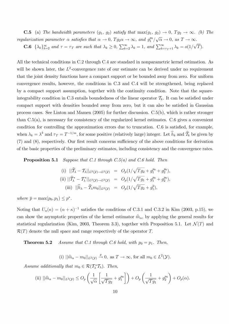
Theorem 5.2 Assume that C.1 through C.6 hold, with p0 = p1. Then,

(i) ||mα −m0||L2(Y)p→ 0, as T →∞, for all m0 ∈ L2(Y).

Assume additionally that m0 ∈ R(T ∗λ Tλ). Then,

(ii) ||mα −m0||L2(Y) ≤ Op

(1√α

[1√Tg2

+ gp01

])+Op

(1√Tg1

+ gp02

)+Op(α).

10

Since Tλ is an integral operator, the condition m0 ∈ R(T ∗λTλ) imposes certain smoothness on m0,

which we call an abstract smoothness condition. When Tλ is a compact operator, it means that the

generalized Fourier coefficients of m0 (with respect to the eigenfunctions) decay fast enough relative

to the eigenvalues of Tλ.3

Remark 5.1. (the Optimal Convergence Rate) Let m0 be any function in R(T ∗λTλ). Suppose

a side condition on (g1, g2) such that (Tg1)−1/2 ≤ O(g

2p0/31 ), and g

3p0/22 ≤ O([Tg2]

−1/2). Then, the

optimal convergence rate of mα is given by

||mα −m0||L2(Y) = Op(T− p03p0+1 ),

under the optimal choice of smoothing parameters such that g∗1T = C0T− 1(4/3)p0+1 , g∗2T = C1T

− 13p0+1 ,

and α∗T = C2T− p03p0+1 .

Theorem 5.3 (uniform convergence rate of mα(x)) Assume that C.1 through C.6 hold ( p0 = p1)

with compactness of the support Y, and that m0 ∈ R([T ∗λ Tλ]µ), with µ ≥ 1. If α = o(1/(log T )c),

for any c > 0, then,

supy∈Y

|mα(y)−m0(y)| = Op

(logT√

α

[1√Tg2

+ gp01

])+Op

(log T

[1√Tg1

+ gp02

])+Op(α log T ).

By using the same argument of Remark 5.1, we can show that the optimal uniform convergence

rate of mα is given by:

supy∈Y

| mα(y)−m0(y) | = Op(T− p03p0+1 log T ), for m0 ∈ R(T ∗λTλ),

where the optimal choice of smoothing parameters are the same as in Remark 5.1. Note that in this

case, the twice-differentiability condition of m and fk implies that

supy∈Y

| mα(y)−m0(y) | = Op(T− 27 log T ) = op(T

−1/4).

5.2 Parametric estimate

We here establish the consistency with rate for the parametric part. With the uniform convergence

rate of mα(·) faster than T−1/4, the derivations are much simpler than those of Theorem 6 and the

discussion in Section 4.4 in Linton and Mammen (2005), since mα does not depend on β. First

define the sample Gaussian quasi-likelihood (upto constants) assuming that m0 is known perfectly,

ℓ(β) =1

T

T∑

t=1

ln σ2t (β, m0) +y2t

σ2t (β, m0),

3As in Tautenhahn (1998) and other papers in this literature we can use the weaker condition that m0 ∈− logR([T ∗λ Tλ]η) for some η > 0 at the cost of a great deal longer proofs.

11

and suppose that β is the unique minimizer of ℓ(β), while β0 is the unique minimizer of E[ℓ(β)].

The properties of β have been well studied in the literature, see for example Lee and Hansen (1994)

and Rahbek and Jensen (2004). In fact under the conditions that make yt strictly stationary and

geometrically mixing we can expect β to be root-T consistent and asymptotically normal.

Theorem 5.4. Assume that C.1 through C.6 hold ( p0 = p1) with compactness of the support Y,

and that m0 ∈ R([T ∗λ Tλ]µ), with µ ≥ 1. Suppose that β is T−1/4-consistent. If α = o(1/(log T )c),

for any c > 0, and if τ †(T ) = c log T, then,

β − β = op(T−1/4).

Under some conditions, one might be able to obtain asymptotic normality at rate root-T from

the arguments of Chen and Shen (1998), but this is not guaranteed see Kim (2003).

6 Numerical Results

For an extensive simulation study of this method applied to a cross-sectional setting, see Kim (2003).

We content ourselves with providing some evidence of the empirical relevance of our model and

assumptions.

6.1 Empirical Application

The assumption that the process {∆y2t } is weakly stationary while y2t cannot be tested by examining

the tail index of the two series. In practice one has to demean the process yt first. We investigate a

sample of daily returns on the S&P500 from 1955 to 2002, a total of 11,893 observations. The tail

index κ of a series Xt is defined as the value for which

1− Pr(Xt > x) ≃ 1− Lx−κ

as x →∞, where L is a constant or a slowly varying function of x. We compute the tail index κ of

an ordered positive series Xt by the Hill (1975) method

1

κ=1

M

M∑

t=1

logXt

XM+1

In Figure 1 we give the Hill plot with 95% confidence interval for y2t .

12

Figure 1. Shows the value of κ against threshold size M for the series y2t .

It is generally above one but less than two implying that E[y2t ] < ∞ but E[y4t ] =∞. The corre-

sponding hill plots for |∆y2t | show slightly lighter tails: we just show the ratio of κ for |∆y2t | to κ for

y2t , which is generally above one.

13

Figure 2. Shows the ratio of κ for the series |∆y2t | to κ for the series y2t against threshold size M.

For these data at least the evidence of integrated process is weak although it does seem that dif-

ferencing reduces the weight of the tails significantly. Our second application is to a high frequency

stock return series with n =4626.

14

Figure 3. Shows the value of κ against threshold size M for the series y2t . High frequency stock

return series.

15

Figure 4. Shows the ratio of κ for the series |∆y2t | to κ for the series y2t against threshold size M.

High frequency stock return series.

In this case, the differencing operation reduces the thickness of the tails considerably. The squared

return series shows some evidence of non existence of first moment, but the differenced series has

much lighter tails.

7 Conclusions

We established the consistency and rate of convergence of our estimates. Unfortunately, the pointwise

distribution theory for m appears to be very difficult and we have not anything to offer on this.

Likewise our theory for β falls short of root-T consistency and asymptotic normality.

16

8 Appendix

Proof of Proposition 4.1 The integral operator Tλ has a degenerate kernel, i.e., fλ(·, ·) is a finite

sum of products of kernel weights on each observation. Noting that Tλ is of a finite rank, the proof

is direct from Proposition 3.1 in Kim (2003), since Tλ : L2(Y) → L2(Y) is uniformly consistent for

Tλ on MY ⊂ L2(Y) s.t. dim(MY ) =∞. �

Lemma A.1. Assume that C.1 through C.5(a) hold. Then, it holds that

(i) supk≥2

||Tk − Tk||2 = Op(g2p01 + g2p02 ) +Op(

1

Tg2),

(ii) supk≥2

||T ∗k − T ∗k ||2 = Op(g2p01 + g2p02 ) +Op(

1

Tg1),

(iii) supk≥2

||hk − Tkm0||2L2(Y) = Op(1

Tg2) +Op(g

2p1 + g2p02 ),

where p = max(p0, p1).

Proof. (i) With a ∗ b denoting convolution of a and b, we define

mc(g1)(y) ≡ (Kg1 ∗m)(y) =

∫Kg1(y − s)m(s)ds, (14)

and

fc(g)k (y, w) ≡ (K(g1,g2) ∗ fk)(y, w) =

∫

Y

∫

YKg1(s1 − y)Kg2(s2 − w)fk(s1, s2)ds1ds2

= E[Kg1(yt−1 − y)Kg2(yt−k − w)].

By adding and subtracting∫

fc(g)k (y, w)m(y)dy, the estimation errors of Tk are decomposed into

(Tkm− Tkm)(w) =1

T ∗

T∑

t=τ+1

∫[Kg1(yt−1 − y)Kg2(yt−k − w)− f

c(g)k (y, w)]m(y)dy

+

∫[f

c(g)k (y, w)− fk(y, w)]m(y)dy

≡ sT (w) + BT (w),

from which we obtain the MISE of Tkm, given by

E

∫

Y

[(Tk − Tk)m

]2(w)dw =

∫

Y

{Var [sT (w)] + E

2 [BT (w)]}

dw.

From

sT (w) =1

T ∗

T∑

t=τ+1

{Kg2(yt−k − w)mc(g1)(yt−1)− E[Kg2(yt−k − w)mc(g1)(yt−1)]

},

17

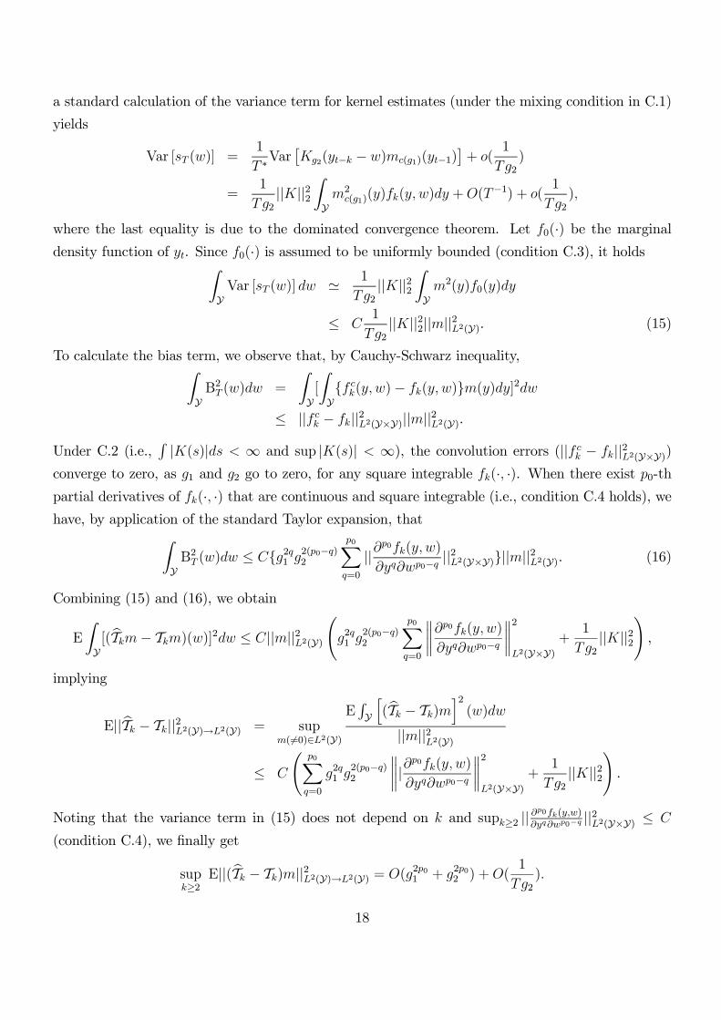
a standard calculation of the variance term for kernel estimates (under the mixing condition in C.1)

yields

Var [sT (w)] =1

T ∗Var[Kg2(yt−k − w)mc(g1)(yt−1)

]+ o(

1

Tg2)

=1

Tg2||K||22

∫

Ym2

c(g1)(y)fk(y, w)dy +O(T−1) + o(

1

Tg2),

where the last equality is due to the dominated convergence theorem. Let f0(·) be the marginal

density function of yt. Since f0(·) is assumed to be uniformly bounded (condition C.3), it holds∫

YVar [sT (w)] dw ≃ 1

Tg2||K||22

∫

Ym2(y)f0(y)dy

≤ C1

Tg2||K||22||m||2L2(Y). (15)

To calculate the bias term, we observe that, by Cauchy-Schwarz inequality,∫

YB2T (w)dw =

∫

Y[

∫

Y{f c

k(y, w)− fk(y, w)}m(y)dy]2dw

≤ ||f ck − fk||2L2(Y×Y)||m||2L2(Y).

Under C.2 (i.e.,∫|K(s)|ds < ∞ and sup |K(s)| < ∞), the convolution errors (||f c

k − fk||2L2(Y×Y))converge to zero, as g1 and g2 go to zero, for any square integrable fk(·, ·). When there exist p0-th

partial derivatives of fk(·, ·) that are continuous and square integrable (i.e., condition C.4 holds), we

have, by application of the standard Taylor expansion, that∫

YB2T (w)dw ≤ C{g2q1 g

2(p0−q)2

p0∑

q=0

||∂p0fk(y, w)

∂yq∂wp0−q ||2L2(Y×Y)}||m||2L2(Y). (16)

Combining (15) and (16), we obtain

E

∫

Y[(Tkm− Tkm)(w)]2dw ≤ C||m||2L2(Y)

(g2q1 g

2(p0−q)2

p0∑

q=0

∥∥∥∥∂p0fk(y, w)

∂yq∂wp0−q

∥∥∥∥2

L2(Y×Y)+

1

Tg2||K||22

),

implying

E||Tk − Tk||2L2(Y)→L2(Y) = supm(�=0)∈L2(Y)

E∫Y

[(Tk − Tk)m

]2(w)dw

||m||2L2(Y)

≤ C

(p0∑

q=0

g2q1 g2(p0−q)2

∥∥∥∥|∂p0fk(y, w)

∂yq∂wp0−q

∥∥∥∥2

L2(Y×Y)+

1

Tg2||K||22

).

Noting that the variance term in (15) does not depend on k and supk≥2 || ∂p0fk(y,w)

∂yq∂wp0−q||2L2(Y×Y) ≤ C

(condition C.4), we finally get

supk≥2

E||(Tk − Tk)m||2L2(Y)→L2(Y) = O(g2p01 + g2p02 ) +O(1

Tg2).

18

(ii) By symmetry of the above arguments, a similar result holds for T ∗k .

(iii) Let r(yt−1) = m0(yt−1)−m0,c(g1)(yt−1), where m0,c(g1)(·) is defined by (14). From (Tkm)(w) =T ∗−1∑T

t=τ+1 Kg2(yt−k − w)mc(g1)(yt−1), we get

(hk − Tkm0)(w)

=1

T ∗

T∑

t=τ+1

Kg2(yt−k − w)ηt +1

T ∗

T∑

t=τ+1

Kg2(yt−k − w)r(yt−1)

=1

T ∗

T∑

t=τ+1

Kg2(yt−k − w)ηt +1

T ∗

T∑

t=τ+1

Kg2(yt−k − w)(νt−1 − νct−1)

+1

T ∗

T∑

t=τ+1

Kg2(yt−k − w)E(r(yt−1)|yt−k)

≡ s1,T (w) + s2,T (w) + BT (w),

where νt−1 = m0(yt−1)− E(m0(yt−1)|yt−k), and νct−1 = m0,c(g1)(yt−1)− E(m0,c(g1)(yt−1)|yt−k).

As a consequence,

E

∫

Y(hk − Tkm0)

2(w)dw =

∫

Y

{Var [s1,T (w) + s2,T (w)] + E

2[BT (w)]}

dw.

By the standard argument in kernel regression, the variance of the main stochastic term is calculated

in a straightforward way:

Var [s1,T (w)] =1

Tg2||K||22E(η2t |yt−k = w)f0(w)(1 + o(1)),

leading to∫

YVar [s1,T (w)] dw =

1

Tg2||K||22

[∫

YE(η2t |yt−k = w)f0(w)dw

](1 + o(1))

=1

Tg2||K||22σ2η(1 + o(1)) = O(

1

Tg2), (17)

where σ2η = E(η2t ). From E[νt−1|yt−k] = E[νc

t−1|yt−k] = 0, it follows that

E[(νt−1 − νct−1)

2|yt−k] = Var[r(yt−1)|yt−k] ≤ E[r2(yt−1)|yt−k],

implying, by the mixing assumption and the law of iterated expectation, that

Var [s2,T (w)] ≃1

T ∗E{[Kg2(yt−k − w)(νt−1 − νc

t−1)]2}

=1

T ∗E{[Kg2(yt−k − w)]2E[r2(yt−1)|yt−k]}

=1

T ∗E{[Kg2(yt−k − w)r(yt−1)]

2}

=1

Tg2||K||22

∫

Yr2(y)fk(y, w)dy(1 + o(1)).

19

From boundedness of f0(·),∫

YVar [s2,T (w)] dw ≃ 1

Tg2||K||22

∫

Yr2(y)f0(y)dy

≤ C

Tg2||K||22||m(·)−mc(g1)(·)||2L2(Y) = o(

1

Tg2),

since the convolution error, ||m(·) −mc(g1)(·)||L2(Y), converges to zero, as g1 → 0. To calculate the

bias term, we note, by the dominated convergence theorem, that

E[BT (w)] = E[Kg2(yt−k − w)r(yt−1)]

=

∫

Y[m(y)−mc(g1)(y)]fk(y, w)dy(1 + o(1)). (18)

Letting fc(g1)k (u, w) =

∫Y Kg1(y − u)fk(y, w)dy, we obtain an alternative form of the bias such that

E[BT (w)] = {∫

Y

[fk(u, w)− f

c(g1)k (u, w)

]m(u)du}(1 + o(1)), (19)

since∫Y mc(g1)(z)fk(z, w)dz =

∫Y f

c(g1)k (u, w)m(u)du, by Fubini’s Theorem. By Cauchy-Schwarz in-

equality, it follows from (18) and (19), together with square-integrability of fk(·, ·) and m(·), that

∫

YE2 [BT (w)] dw ≤ Cmin{||m(·)−mc(g1)(·)||2, ||fk(·)− f

c(g1)k (·)||2},

which, by the standard method of Taylor expansion (under C.4 ), gives

∫

YE2 [BT (w)] dw = O(g

max{2p0,2p1}1 + g2p02 ).

Since the variance term in (17) dose not depend on k and supk≥2 ||dp1m(y)dyp1

||2L2(Y) ≤ C (condition C.4),

it holds that

supk≥2

E

∫

Y(hk − Tkm0)

2(w)dw = O(1

Tg2) +O(g2p1 + g2p02 ),

�

Proof of Proposition 5.1. (i) By the triangle inequality,

||Tλ − Tλ||L2(Y)→L2(Y) ≤τ∑

k=2

λk||Tk − Tk||L2(Y)→L2(Y) +∞∑

k=τ+1

λk||Tk||L2(Y)→L2(Y)

≤ C{supk≥2

||Tk − Tk||L2(Y)→L2(Y) + o(1/√

T )},

where the second inequality follows from supk≥2 ||Tk|| ≤ supk≥2 ||fk|| ≤ C (condition C.3) and∑∞

k=τ+1 λk = o(1/√

T ) (condition C.6). Now, the proof is immediate from Lemma A.1(i).

20

The proof of (ii) can be shown in the same way.

(iii) Note that

||hλ − Tλm0|| ≤τ∑

k=2

λk||hk − Tkm0|| ≤ supk≥2

||hk − Tkm0|| ,

since∑τ

k=2 λk ≤∑∞

k=2 λk = 1. The proof follows, if we apply Lemma A.1(iii). �

Before proving the main results, we need to introduce some useful lemmas that are borrowed

from Kim (2003). First, note that Uα(κ) = (α+ κ)−1 satisfies the following conditions:

B.1 Let κ ≡ supn≥n0 ||T ∗λ Tλ||L2(Y)→L2(Y). A parameter dependent family of continuous func-

tions, {Uα(·)}α>0, defined on (0, κ], satisfy that (i) supκ∈(0,κ] |Uα(κ)κ| ≤ C < ∞, for α > 0, (ii)

limα→0+ Uα(κ) =1κ, for all κ ∈ (0, κ], and (iii) supκ∈(0,κ] |Uα(κ)| = O( 1

α), as α → 0+.

B.2 Given Uα : (0, κ]→ R, it holds for any µ ∈ (0, 1] that supκ∈(0,κ] κµ|Uα(κ)κ− 1| ≤ Cαµ, for

any α ∈ (0, α0), where α0 > 0.

Lemma A.2 If α = α(T )→ 0 as T →∞, then:

(i) ||Uα(T ∗λ Tλ)||L2(Y)→L2(Y) = Oa.s(α−1),

(ii) ||Uα(T ∗λ Tλ)T ∗λ ||L2(Y)→L2(Y) = Oa.s(√

α−1),

Assume additionally that Tλ : L2(Y)→ L2(Y) converges pointwise, in probability, to Tλ : L2(Y)→L2(Y), which is bounded and one-to-one. Then,

(iii) ||[Uα(T ∗λ Tλ)T ∗λ Tλ − I]m||L2(Y) = op(1), for all m ∈ L2(Y).

Proof Since Uα(·) satisfies B.1 and Tλ has a finite rank, the results are immediate from Lemma

3.2 (Kim 2003, p.41). �

Lemma A.3 Let G : L2(Y)→ L2(Y) be a linear bounded operator and G∗ : L2(Y)→ L2(Y) be

adjoint to G. Then, for all m ∈ L2(Y),

(i) ||[Uα(G∗G)G∗G− I](G∗G)µ||L2(Y)→L2(Y) ≤ Cαmin(µ,1), for µ > 0.

(ii) ||[Uα(G∗G)G∗G− I]G∗||L2(Y)→L2(Y) ≤ Cα1/2, for µ > 0.

Proof. Since Uα satisfies B.2, the results follow from Lemma 3.3 (Kim 2003, p.42). See also

Carrasco, Florens and Renault (2006). �

21

For MT (Y) = {m ∈ M(Y) : mT (x) = T ∗−2KYT (x)

⊤

bT , for bT ∈ RT∗}, we define (T ∗λ Tλ)ω|MT:

MT → C(Y) to be the restriction (into MT ) of (T ∗λ Tλ)ω : L2(Y)→ C(Y), where C(Y) is a space of

continuous functions defined on Y.

Lemma A.4. Assume that fk(·, ·) is a uniformly consistent estimate of fk(·, ·) which is con-

tinuous with a compact support. Then,(T ∗λ Tλ)ω|MT:MT → C(Y) is uniformly bounded in the sense

that

||(T ∗λ Tλ)ω|MT||L2(Y)→C(Y) = sup

m∈MT

supx∈Y

|(T ∗λ Tλ)ωm(x)|||m||L2(Y)

= Op(1),

where 0 < ω ≤ 1.

Proof. By applying Uniform Boundedness Principle (or, the Banach-Steinhaus principle), the

assertion follows, if we show that, for each mT ∈MT ⊂ L2(Y) with ||m||L2(Y) = 1,

supx∈Y

|(T ∗λ Tλ)ωmT (x)| = Op(1).

Observing that QY,λ is symmetric nonnegative semi-definite, we can show that, for mT (·) ∈MT (Y),

supx∈Y

|(T ∗λ Tλ)ω|MTmT (x)| = sup

x∈Y|T ∗−2KY

T (x)⊤

M1/2λ Qω

Y,λM−1/2λ bT |

≤ C supx∈Y

|T ∗−2KYT (x)

⊤

M1/2λ QY,λM

−1/2λ bT |

= C supx∈Y

|(T ∗λ Tλ)|MTmT (x)|, for all T .

By the Cauchy-Schwarz (CS) inequality and boundedness of fk(·, ·), it holds that

supx| (T ∗λ Tλ − T ∗λ Tλ)mT (x)|

= supx|∫

Y

∫

Y

τ∑

k=2

τ∑

l=2

λkλl[fk(x, w)fl(z, w)− fk(x, w)fl(z, w)]mT (z)dwdz|

+∞∑

k=τ+1

∞∑

l=τ+1

λkλl

∫

Y

∫

Y|fk(x, w)fl(z, w)mT (z)|dwdz

≤ supx

τ∑

k=2

τ∑

l=2

λkλl||fk(x, ·)fl(·, ·)− fk(x, ·)fl(·, ·)||L2(Y)×L2(Y)||mT ||L2(Y) + C∞∑

k=τ+1

∞∑

l=τ+1

λkλl

≤ C supx,z,w

τ∑

k=2

τ∑

l=2

λkλl|fk(x, w)fl(z, w)− fk(x, w)fl(z, w)| + o(1) = op(1),

where the last inequality comes from the compact support assumption, uniform consistency of the

kernel density estimate fk(·, ·), and condition C.6. In a similar way, we can show, by the CS inequality

22

and boundedness of fk(·, ·), that, for any m ∈ L2(Y),

supx|T ∗λ Tλm(x)| ≤ sup

x

∞∑

k=2

∞∑

l=2

λkλl||fk(x, ·)fl(·, ·)||L2(Y)×L2(Y)||mT ||L2(Y)

≤ C supx,z,w

∞∑

k=2

∞∑

l=2

λkλl|fk(x, w)fl(z, w)| < ∞.

Hence, it follows that

supx| T ∗λ TλmT (x)| ≤ C sup

x| T ∗λ TλmT (x)| < ∞,

implying that

supx∈Y

|(T ∗λ Tλ)ωmT (x)| < ∞,

as required. �

Proof of Theorem 5.2. (i) We use the following error decomposition

mα −m0 = Uα(T ∗λ Tλ)T ∗λ (hλ − Tλm0) + [Uα(T ∗λ Tλ)T ∗λ Tλ − I]m0. (20)

By Proposition 5.1(i), Tλ : L2(Y) → L2(Y) is a consistent estimator for the true operator Tλ :L2(X )→ L2(W) which is bounded and one-to-one. Also, under the bandwidth conditions in C.5, it

holds by Proposition 5.1(iii) that ||hλ−Tλm0||L2(Y)/√

αp→ 0, as T →∞. Now, the assertion follows,

by Lemma A.2(ii) and (iii) to (20).

(ii) Let m1 = (T ∗λ Tλ)−1m0. The error decomposition in this case takes form of

Uα(T ∗λ Tλ)T ∗λ (hλ − Tλm0) + [(Uα(T ∗λ Tλ)T ∗λ Tλ − I)T ∗λ Tλ]m1

−[(Uα(T ∗λ Tλ)T ∗λ Tλ − I)T ∗λ ](Tλ − Tλ)m1 − (Uα(T ∗λ Tλ)T ∗λ Tλ − I)(T ∗λ − T ∗λ )Tλm1.

By Lemma A.2(ii), L2-norm of the first term is bounded by C1√α||hλ− Tλm0||L2(W), almost surely. By

applying Lemma A.3(i) and (ii), we get:

||(Uα(T ∗λ Tλ)T ∗λ Tλ − I)T ∗λ Tλ|| ≤ Cα, a.s

||(Uα(T ∗λ Tλ)T ∗λ Tλ − I)T ∗λ || ≤ Cα1/2, a.s.

Also, by A.2.(iii), it holds that (Uα(T ∗λ Tλ)T ∗λ Tλ− I) ≤ C, which, together with the results of Propo-

sition 5.1, completes the proof. �

23

Proof of Theorem 5.3 Let m1 = (T ∗λ Tλ)−1m0. From the proof of Theorem 5.2(ii),

Uα(T ∗λ Tλ)T ∗λ (hλ − Tλm0) + [Uα(T ∗λ Tλ)T ∗λ Tλ − I]T ∗λ Tλm1

−[Uα(T ∗λ Tλ)T ∗λ Tλ − I]T ∗λ (Tλ − Tλ)m1

−Uα(T ∗λ Tλ)T ∗λ Tλ(T ∗λ − T ∗λ )Tλm1 + (T ∗λ − T ∗λ )Tλm1

≡ ξ1T + ξ2T + ξ3T + ξ4T + ξ5T .

Let ω > 0 be any fixed real number. In the proof of Theorem 4.2 (step II), we showed the spectral

representation of r(T ∗λ Tλ) from which follows

(T ∗λ Tλ)ωm(x) = T ∗−2KYT (x)

⊤

M1/2λ Qω−1

Y,λ M1/2λ < KY

T , m >L2(Y) .

Since, for each T , (T ∗λ Tλ)ωm is a continuous function for any m ∈ L2(Y), it holds that

R[(T ∗λ Tλ)ω] ⊂ C(Y), for each T ,

i.e., (T ∗λ Tλ)ω : L2(Y)→ C(Y) is well defined. Let MT (Y) = {m ∈ L2(Y) : mT (x) = T−2KYT (x)

⊤

bT ,

for bT ∈ RT}. Define (T ∗λ Tλ)ω|MT:MT → C(Y). Note that, under the given conditions, fk(·, ·) is the

uniformly consistent estimate of fk(·, ·). Consequently, by Lemma A.4, (T ∗λ Tλ)ω|MT:MT → C(Y) is

uniformly bounded in the sense that

||(T ∗λ Tλ)ω|MT||L2(Y)→C(Y) = sup

m∈MT

supx∈Y

|T ∗λ Tλm(x)|||m||L2(Y)

= Op(1).

From the definition of the operator norm and R{Uα(T ∗λ Tλ)(T ∗λ Tλ)−ωT ∗λ } ⊂MT , we obtain

supx∈Y

|ξ1T (x)|

= supx∈Y

|Uα(T ∗λ Tλ)T ∗λ (hλ − Tλm0)(x)|

= supx∈Y

|(T ∗λ Tλ)ω[Uα(T ∗λ Tλ)(T ∗λ Tλ)−ωT ∗λ (hλ − Tλm0)](x)|

≤ ||(T ∗λ Tλ)ω|MT||L2(Y)→C(Y)||Uα(T ∗λ Tλ)(T ∗λ Tλ)−ωT ∗λ ||L2(Y)→L2(Y)||hλ − Tλm0||L2(Y)

≤ Cα−1/2−2ω||hλ − Tλm0||L2(Y) = Op(α−1/2−2ω[1/

√Tg2 + gp0

1 ]), for any ω > 0,

where the last equality comes from Proposition 5.1. Since we assume that α = o(1/(log T )c), for any

c > 0, we get, by letting c = 1/2ω,

supx∈Y

|ξ1T (x)| = Op(α−1/2[1/

√Tg2 + gp0

1 ] log T ).

24

By the same arguments, we have

supx∈Y

|ξ4T (x)| = supx∈Y

|(T ∗λ Tλ)ω[Uα(T ∗λ Tλ)(T ∗λ Tλ)1−ω(T ∗λ − T ∗λ )Tλm1](x)|

≤ ||(T ∗λ Tλ)ω|MT||L2(Y)→C(Y)||Uα(T ∗λ Tλ)(T ∗λ Tλ)1−ω||L2(Y)→L2(Y)||(T ∗λ − T ∗λ )Tλm1||L2(Y)

= Op(α−ω[1/

√Tg1 + gp0

1 + gp02 ]) = Op([1/

√Tg1 + gp0

1 + gp02 ] log T ),

supx∈Y

|ξ2T (x)| = supx∈Y

|(T ∗λ Tλ)ω{[Uα(T ∗λ Tλ)T ∗λ Tλ − I](T ∗λ Tλ)1−ωm1}(x)|

≤ ||(T ∗λ Tλ)ω|MT||L2(Y)→C(Y)||[Uα(T ∗λ Tλ)T ∗λ Tλ − I](T ∗λ Tλ)1−ω||L2(Y)→L2(Y)||m1||L2(Y)

≤ Cα1−2ω||m1||L2(Y) = Op(α log T ),

and

supx∈Y

|ξ3T (x)| = supx∈Y

|(T ∗λ Tλ)ω{[Uα(T ∗λ Tλ)T ∗λ Tλ − I](T ∗λ Tλ)−ωT ∗λ (Tλ − Tλ)m1}(x)|

≤ ||(T ∗λ Tλ)ω|MT||L2(Y)→C(Y)||[Uα(T ∗λ Tλ)T ∗λ Tλ − I](T ∗λ Tλ)−ωT ∗λ ||L2(Y)→L2(Y)||(Tλ − Tλ)m1||L2(Y)

≤ Cα1/2−2ω||(Tλ − Tλ)m1||L2(Y) = Op(α1/2[1/

√Tg2 + gp0

1 + gp02 ] log T ).

For the uniform convergence rate of ξ4T (x) = (T ∗λ − T ∗λ )h1, we note that T ∗λ h1 is equivalent (up

to some bias term) to the standard one-dimensional kernel estimate, where h1 = Tλm1. Hence, its

uniform convergence rate follows from application of Masry (1996)4:

supx∈Y

|ξ3T (x)| = Op([1/√

Tg1 + gp01 + gp0

2 ] logT ).

�

Proof of Theorem 5.4. First, we show that β is consistent, which follows from the consistency

of β and the uniform approximation of ℓ(β) by ℓ(β) over B. Then, we establish that ℓ(β) − ℓ(β) =

op(T−1/4) uniformly over a shrinking neighborhood of β0. The argument is fairly standard so we just

sketch the second part here. We have

|ℓ(β)− ℓ(β)| ≤ 1

T

T∑

t=1

∣∣∣∣lnσ2t (β, mα)

σ2t (β, m0)

∣∣∣∣+1

T

T∑

t=1

y2t|σ2t (β, mα)− σ2t (β, m0)|

σ2t (β, m0)σ2t (β, mα)(21)

where

maxτ†≤t≤T

∣∣σ2t (β, mα)− σ2t (β, m0)∣∣ ≤

∞∑

j=1

βj−1 supy∈Y

|mα(y)−m0(y)|

+∞∑

j=τ†+1

βj−1[(1− β) maxτ†≤t≤T

y2t−j + maxτ†≤t≤T

m(yt−j)]

= op(T−1/4),

4More rigorously, we may follow the same line of the proof of Proposition 3.1(ii) to apply the uniform convergence

results in Masry (1996).

25

since ys and m(ys) are bounded by assumption. Using ln(1 + δ) ≤ |δ| for |δ| < 1, we can bound the

first term in (21) with probability tending to one by

∣∣∣∣∣1

T

T∑

t=1

lnσ2t (β, mα)

σ2t (β, m0)

∣∣∣∣∣ ≤1

T

T∑

t=1

∣∣∣∣σ2t (β, mα)− σ2t (β, m0)

σ2t (β, m0)

∣∣∣∣ = op(T−1/4),

since minτ†≤t≤T σ2t (β, m0) is bounded away from zero. Likewise the second term in (21) is op(T−1/4).

References

[1] A , C. ��� X. C��� (2003): “Efficient estimation of models with conditional moment restric-

tions containing unknown functions,” Econometrica 71(6), 1795-1844.

[2] B ���, M. ��� M. S������ (1980): Quantitative Analysis in Sobolev Imbedding Theo-

rems and Applications to Spectral Theory. American Math. Soc. Tran., series 2, Vol 114.

[3] B�������, R., X. C���, ��� D. K ������� (2004): “Semiparametric Estimation of Shape

Invariant Engle Curves under Endogeneity” CEMMAP working paper WP15/03

[4] B�������, R. ��� J. L. P�"��� (2001a): “Endogeneity in nonparametric and semipara-

metric regression models,” forthcoming in Advances in Econometrics, Proceedings of the World

Meetings, 2000, ed. by L. Hansen, North Holland.

[5] B�������, R. ��� J. L. P�"��� (2001b): “Endogeneity in semiparametric binary response

models,” Center for Microdata Methods and Practice, Working Paper, 05/01.

[6] C���#�, M., J.P. F�����, ��� E. R������ (2006), “Linear Inverse problems in Struc-

tural Econometrics,” Handbook of Econometrics, volume 6, eds. J.J. Heckman and E. Leamer.

[7] C���, X. ��� X. S��� (1998). Sieve extremum estimates for weakly dependent data. Econo-

metrica 66, 289-314.

[8] D������, S., J-P. F�����, ��� E. R������ (2001): “Nonparametric instrumental re-

gression, Working Paper, GREMAQ, University of Toulouse.

[9] D��, M. (1999): “Instrumental variable estimation of models with discrete endogenous regres-

sors, ” presented at 2000 World Congress of the Econometric Society.

[10] E�&�, H. (1987): “On the choice of the regularization parameter for iterated Tikhonov regu-

larization of ill-posed problems,” Journal of Approximation Theory 49, 55-63.

26

[11] E�&�, H. ��� H. G)�� (1988): “A posteriori parameter choice for general regularization

methods for solving linear ill-posed problems,” Applied Numerical Mathematics 4, 395-417.

[12] E�&��, R.F., ��� T. B�������+ (1986): “Modelling the persistence of Conditional Vari-

ances,” Econometric Reviews 5, 1-50.

[13] E�&��, H.W., M. H���, ��� A. N��.��� (2000): Regularization of Inverse Problems.

Dordrecht: Kluwer Academic Press.

[14] F��, J. (1991): “Global behavior of deconcovolution kernel estimates,” Statistica Sinica 1, 541-

551.

[15] G����#�, C.W. (1993): Inverse Problems in the Mathematical Sciences. Braunschweig:

Vieweg.

[16] G����#�, C.W. (1983): “On the Asymptotic Order of Accuracy of Tikhonov Regularization,”

Journal of Optimization Theory and Applications 41, 293-298.

[17] G����#�, C.W. (1977): Generalized Inverses of Linear Operators: Representation and Ap-

proximation. New York: Dekker.

[18] H��� P. ��� C.C. H�/�� (1980): Martingale Limit Theory andIts Applications. Academic

Press, New York.

[19] H��� P. ��� J. L. H��" �0 (2005): “Nonparametric methods for inference in the presence

of instrumental variables,” The Annals of Statistics .

[20] H����� L. P. (1982): “Large sample properties of generalized method of moments estimators,”

Econometrica 50, 1029-1054.

[21] H�+�/, A., E. R� 0, ��� N. S������ (1994): “Multivariate Stochastic Variance Models,”

Review of Economic Studies 61, 247-64.

[22] H ��, B. M. (1975), A Simple General Approach to Inference about the Tail of a Distribution,

Annals of Statistics 3, 1163-1174.

[23] H�����, V. ��� J. S. P/� (1980): Applications of Functional Analysis and Operator Theory.

London: Academic Press.

[24] I�.���, G. W. ��� W. K. N�"�/ (2001): “Identification and estimation of triangular simul-

taneous equations models without additivity, Working Paper.

27

[25] I+���+, V.K., V.V. V�� �, ��� V.P. T����� (1978): Theory of Linear Ill-Posed Problems.

Moscow: Nauka.

[26] K �, W. (2003): “Identification and Estimation of Nonparametric Structural mod-

els by Instrumental Variables Method,” Manuscript, Humboldt University. Available at

http://ideas.repec.org/p/ecm/feam04/733.html.

[27] K �&, J.T. ��� D. C� �� �&"��� (1979): “Approximation of generalized inverses by iter-

ated regularization,” Numerical Functional Analyses and Optimizations 1, 499 -513.

[28] K �#�, A. (1996): An Introduction to the Mathematical Theory of Inverse Problems. New

York: Springer Verlag.

[29] K���, R. (1989): Linear Integral Equations. Berlin: Springer Verlag.

[30] L��, S., ��� H�����, B. (1994): “Asymptotic Theory for the GARCH(1,1) Quasi-Maximum

Likelihood Estimator,” Econometric Theory, 10, 29-52.

[31] L ����, O. B. ��� E. M����� (2005): “Estimating semiparametric ARCH(∞) models by

kernel smoothing methods,” Econometrica 73, 771-836.

[32] M�����, E., O. B. L ����, ��� J. N ����� (1999): “The existence and asymptotic prop-

erties of a backfitting projection algorithm under weak conditions,” The Annals of Statistics,

27(5), 1443-1490.

[33] M��/, E. (1996), “Multivariate local polynomial regression for time series: Uniform strong

consistency and rates,” Journal of Time Series Analysis 17, 571-599.

[34] M� �0, M. ��� P. S� ���� (2004). Ergodicity, mixing, and existence of moments for a

class of Markov models with applications to GARCH and ACD models. Manuscript, Stockholm

School of Economics.

[35] N�����, M.Z. (1976): Generalized Inverses and Applications. New York: Academic Press.

[36] N�����, M.Z. ��� G. W��.� (1974): “Convergence rates of approximate least squares

solutions of linear integral and operator equations of the first kind,” Mathematics of Computation

28(125), 69-80.

[37] N�����, D. (1990). Stationarity and persistence in the GARCH(1,1) models. Econometric

Theory 6, 318-334.

28

[38] N�"�/ W. K. ��� J. L. P�"��� (1988): “Nonparametric instrumental variables estimation,”

MIT Working Paper.

[39] N�"�/ W. K. ��� J. L. P�"��� (2003): “Instrumental variable estimation of nonparametric

models,” Econometrica 71(5), 1565-1578.

[40] N�"�/W. K., J. L. P�"���, ��� F. V���� (1999): “Nonparametric estimation of triangular

simultaneous equations models,” Econometrica 67, 565-603.

[41] N/#��, D. ��� D. C�� (1989): “Convergence rates for regularized solutions of integral

equations from discrete noisy data,” The Annals of Statistics, 17(5), 556-572.

[42] O’S��� +��, F. (1986): “Ill-posed inverse problems (with Discussion),” Statistical Science, 4,

503-527.

[43] P� �� ��, D.L. (1962): “A technique for the numerical solution of certain integral equations of

the first kind,” Journal of the Association for Computing Machinery 9, 84-97.

[44] P����, R. ��� G. V� � � (1990): “On the regularization of projection methods for solving

ill-posed problems,” Numerische Mathematik 57, 63-79.

[45] R��.�, A. ��� S.T. J����� (2004): “Asymptotic normality for Nonstationary, Explosive

GARCH ,” Econometric Theory 20, 1203-1226.

[46] R��� &, C. S. (1988): “Conditions for Identification in Nonparametric and Parametric Mod-

els,” Econometrica, 55, 875-891.

[47] S�&��, J. D. (1958): “The estimation of economic relationships using instrumental variables,”

Econometrica 26, 393-415.

[48] S#��#, E. (1985): “Approximate solution of ill-posed equations: Arbitrarily slow convergence

vs superconvergence, in Constructive Methods for the Practical Treatment of Integral Equations

(edited by G. Hämmerlin and K.H. Hoffmann), pp. 234-243, Basel: Birkhäuser.

[49] S��"���� D. (1967): “Representation and computation of the pseudoinverse,” Proc. Amer.

Math. Soc. 18, 584-586.

[50] S �+����, B.W. (1978): “Weak and strong uniform consistency of the kernel estimate of a

density and its derivatives,” Annals of Statistics Vol.6, No.1, 177-184.

[51] T���������, U. (1998): “Optimality for ill-posed problems under general source conditions,”

Numerical Functional Analyses and Optimizations 19, 377 -398.

29

[52] T�� �, H. (1953): Repeated Least Squares Applied to Complete Equation Systems, The Hague;

Central Planning Bureau.

[53] T ����+, A.N. ��� V. A��� � (1977): Solutions of Ill-Posed Problems. New York: Wiley.

[54] T ����+, A.N (1963): “Solution of incorrectly formulated problems and the regularization

method,” Soviet Mathematics Doklady 4, 1035-1038.

[55] V� � �, G.M. ��� A.Y. V������ �+ (1986): Iteration Procedures in Ill-Posed prob-

lems. 1st Ed. Moscow: Nauka.

[56] +�� R�� �, A.C.M., ��� F.H. R�/�&��� (1999): “On inverse estimation,” in Asymptotics,

Nonparametrics, and Time Series, ed. by S. Ghosh. New York: Marcel Dekker, 579-613.

30