Embed Size (px)
Citation preview
Measuring Mobility∗
by
Frank A. Cowell†
and
Emmanuel Flachaire‡
April 2011
The Suntory Centre Suntory and Toyota International Centres for Economics and Related Disciplines London School of Economics and Political Science Houghton Street London WC2A 2AE
PEP 09 Tel: (020) 7955 6674
∗ We are grateful for helpful comments from Guillermo Cruces, Abigail McKnight, Dirk Van de gaer, Polly Vizard and seminar participants at STICERD and the University of Geneva. † STICERD, London School of Economics, Houghton Street, London, WC2A 2AE, UK, email: [email protected] ‡ GREQAM, Aix-Marseille University, Centre de la Vieille Charité, 2, rue de la Charité, 13236 Marseille cedex 02, France, email: [email protected]

Abstract
Our new approach to mobility measurement involves separating out the valuation of positions in terms of individual status (using income, social rank, or other criteria) from the issue of movement between positions. The quantification of movement is addressed using a general concept of distance between positions and a parsimonious set of axioms that characterise the distance concept and yield a class of aggregative indices. This class of indices induces a superclass of mobility measures over the different status concepts consistent with the same underlying data. We investigate the statistical inference of mobility indices using two well-known status concepts, related to income mobility and rank mobility. Keywords: Mobility measures, axiomatic approach, bootstrap JEL codes: D63

Public Economics Programme The Public Economics Programme was established in 2009. It is located within the Suntory and Toyota International Centres for Economics and Related Disciplines (STICERD) at the London School of Economics and Political Science. The programme is directed by Frank Cowell and Henrik Kleven. The Discussion Paper series is available free of charge. To subscribe to the PEP paper series, or for further information on the work of the Programme, please contact our Research Secretary, Leila Alberici on: Telephone: UK+20 7955 6674 Fax: UK+20 7955 6951 Email: [email protected] Web site: http://sticerd.lse.ac.uk/PEP © Authors: Frank A. Cowell and Emmanuel Flachaire. All rights reserved. Short sections of text, not to exceed two paragraphs, may be quoted without explicit permission provided that full credit, including © notice, is given to the source.
1 Introduction
Mobility is an important concept in several branches of social science and economics. Theway it has been conceived has, to some extent, depended on the particular applicationor even the particular data set under consideration. So, di�erent parts of the literaturehave focused on income or wealth mobility, wage mobility, educational mobility, mobilityin terms of social class. As a consequence of this diversity, the measurement of mobilityis an intellectual problem that has been addressed from many di�erent standpoints.1
Mobility measures are sometimes de�ned, explicitly or implicitly, in relation to a speci�cdynamic model,2 sometimes as an abstract distributional concept similar to inequality,polarisation, dispersion and so on.
This paper focuses on the second interpretation of mobility measurement - mobilitymeasures in the abstract. It develops an approach that is su�ciently �exible to coverincome or wealth mobility on the one hand and, on the other, various types of �rank�mobility where the underlying data are categorical. Our approach separates out thefundamental components of the mobility-measurement problem, proposes an axiomaticframework for the core theoretical issues and examines the statistical properties of severalclasses of measures that emerge from the implementation of the theory.
In the extensive literature mobility is characterised either in terms of one's incomeor in terms of one's position in the distribution, or sometimes both. In some approachesthe distinction between mobility and income volatility - movement of incomes (Fieldsand Ok 1999b) - becomes a little fuzzy. This is perhaps a mistake since mobility isessentially something that characterises society, or the individual's relationship to thesociety (Dardanoni 1993), whereas volatility can be seen as something that relates just toan individual; mobility would be meaningless for Robinson Crusoe, but income volatilitymight be very important.
In the light of this the essential ingredients for a theory of mobility measurement areas follows:
1. a time frame of two or more periods;
2. a measure of an individual's status within society;
3. an aggregation of changes in individual status over the time frame.
In this paper we consider a standard two-period problem and focus on the interplaybetween ingredients 2 and 3, the status measure and the basis for aggregation of move-ments.
A brief word on the notion of �status� is important here. Status may be de�ned in avariety of ways, depending on the focus of interest of a particular mobility study. It couldbe something that is directly observable and measurable for each individual, independentof information about anyone else, a person's income or wealth, perhaps. Alternatively itcould be that a person's status is only well de�ned in relation to information about others- one's location in the income distribution, for example. Our approach is su�ciently�exible to cover either of these interpretations, as we will explain in detail in Section 2.
1For a survey see Fields and Ok (1999a).2See, for example, Atoda and Tachibanaki (1991), Bénabou and Ok (2001).
2

Because mobility is inherently quite a complex phenomenon it is common to �ndthat the phenomenon is broken down into constituent parts, for example into structuraland exchange mobility.3 However, this traditional breakdown is not so important here.What is crucial in our approach is the notional separation of the status concept from theaggregation method (see above). Nevertheless, there is a link to the structural/exchangedistinction as presented in the literature. Exchange mobility can be characterised as atype of average of individual distances �travelled� in the reranking process (Ayala andSastre 2008, Van de gaer et al. 2001).4 The method of aggregation that we will applyis also based on an elementary distance concept that could have a similar natural inter-pretation in terms of exchange mobility. As a consequence, di�erent implementationsof our classes of mobility measure would allow di�erent ways of breaking down overallmobility into exchange and structural mobility.
The paper is organised as follows. Section 2 sets out in more detail the basic ideasunderlying our approach. Section 3 contains the theoretical foundations of the approachand the formal derivation of a �superclass� - a collection of classes - of mobility indices.The properties of the superclass are discussed in Section 4 and statistical inference forkey members of the superclass are discussed in section 5. Section 7 concludes.
2 The Approach: Individual status and mobility
As suggested in the introduction we need very few basic concepts to set out our ap-proach. We will assume that there is some quantity, to be called �income,� that iscardinally measurable and interpersonally comparable. However, this is used only as adevice to show the range of possibilities with our approach; in fact the informationalrequirements for our approach are very modest: only ordinal data are required. Weneed to characterise in a general way a set of classes and a way of representing indi-vidual movements between the classes. So the word �income� here is just a convenientshorthand for initiating the discussion; in what follows �income� can be replaced withany other quantity that is considered to be interpersonally comparable.
Let there be an ordered set of K income classes; each class k is associated withincome level xk where xk < xk+1, k = 1, 2, ..., K − 1. Let pk ∈ R+ be the size of classk, k = 1, 2, ..., K and
K∑k=1
pk = n,
where n is the size of the population. Let k0 (i) be the income class occupied by personi; then the information about a distribution is completely characterised by the vector(xk0(1), ..., xk0(n)
). Clearly this includes the special case where classes are individual
incomes if pk = 0 or 1 in each class and the individual is assumed to be at the lowerbound of the class.
3For an illuminating discussion see Van Kerm (2004). On the de�nition of exchange mobility seeTsui (2009),
4Several ad hoc measures of income mobility pursue the idea of average distance (Mitra and Ok1998). Fields and Ok (1996, 1999b) proposed a mobility index whose distance concept is based on theabsolute di�erences of logarithms of incomes.
3
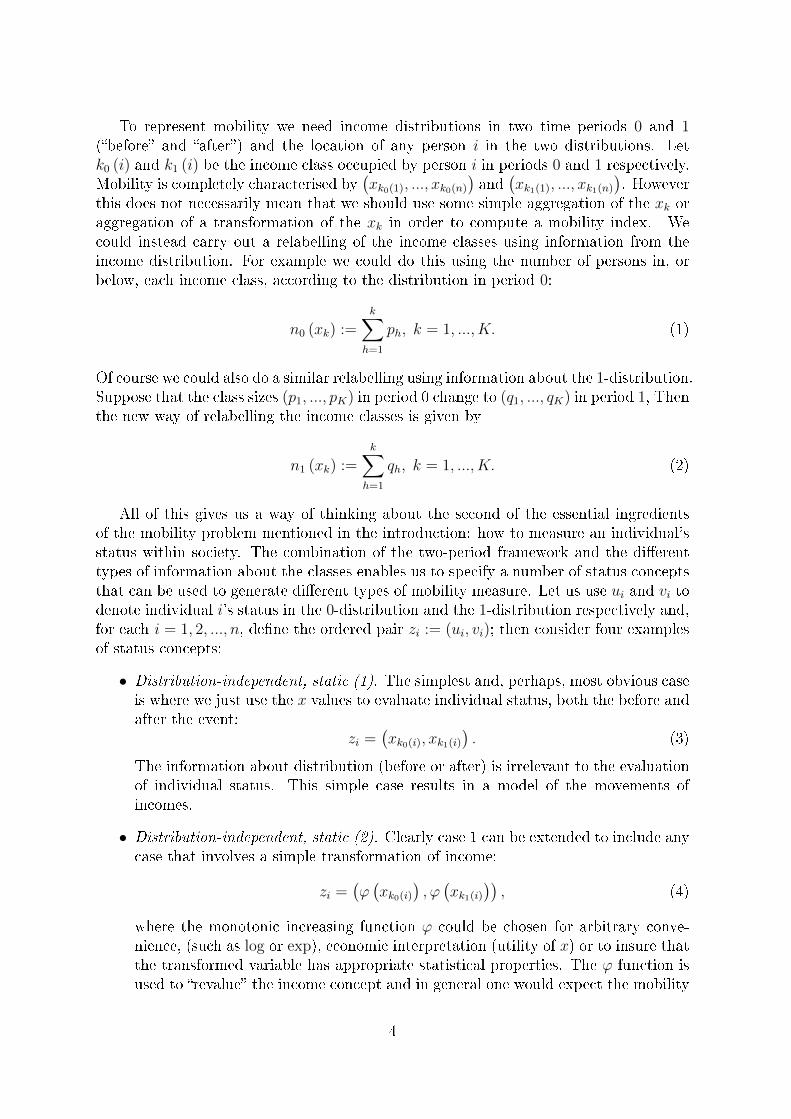
To represent mobility we need income distributions in two time periods 0 and 1(�before� and �after�) and the location of any person i in the two distributions. Letk0 (i) and k1 (i) be the income class occupied by person i in periods 0 and 1 respectively.Mobility is completely characterised by
(xk0(1), ..., xk0(n)
)and
(xk1(1), ..., xk1(n)
). However
this does not necessarily mean that we should use some simple aggregation of the xk oraggregation of a transformation of the xk in order to compute a mobility index. Wecould instead carry out a relabelling of the income classes using information from theincome distribution. For example we could do this using the number of persons in, orbelow, each income class, according to the distribution in period 0:
n0 (xk) :=k∑
h=1
ph, k = 1, ..., K. (1)
Of course we could also do a similar relabelling using information about the 1-distribution.Suppose that the class sizes (p1, ..., pK) in period 0 change to (q1, ..., qK) in period 1, Thenthe new way of relabelling the income classes is given by
n1 (xk) :=k∑
h=1
qh, k = 1, ..., K. (2)
All of this gives us a way of thinking about the second of the essential ingredientsof the mobility problem mentioned in the introduction: how to measure an individual'sstatus within society. The combination of the two-period framework and the di�erenttypes of information about the classes enables us to specify a number of status conceptsthat can be used to generate di�erent types of mobility measure. Let us use ui and vi todenote individual i's status in the 0-distribution and the 1-distribution respectively and,for each i = 1, 2, ..., n, de�ne the ordered pair zi := (ui, vi); then consider four examplesof status concepts:
• Distribution-independent, static (1). The simplest and, perhaps, most obvious caseis where we just use the x values to evaluate individual status, both the before andafter the event:
zi =(xk0(i), xk1(i)
). (3)
The information about distribution (before or after) is irrelevant to the evaluationof individual status. This simple case results in a model of the movements ofincomes.
• Distribution-independent, static (2). Clearly case 1 can be extended to include anycase that involves a simple transformation of income:
zi =(ϕ(xk0(i)
), ϕ(xk1(i)
)), (4)
where the monotonic increasing function ϕ could be chosen for arbitrary conve-nience, (such as log or exp), economic interpretation (utility of x) or to insure thatthe transformed variable has appropriate statistical properties. The ϕ function isused to �revalue� the income concept and in general one would expect the mobility
4

index to be dependent upon the choice of ϕ; this amounts to requiring that mobil-ity be characterised as a cardinal concept. But such an approach is inappropriatefor some types of mobility problem: if one is studying social status or educationalattainment then one particular cardinalisation may appear to be rather arbitrary.To require that a mobility index be based on purely ordinal concepts - to be inde-pendent of the cardinalisation ϕ - might seem rather demanding and to require asomewhat vague approach to the measurement problem. However there is a wayforward that, as we will see, leads to sharp conclusions. This way forward uses thedistribution itself as a means of valuing the K classes; there are two importantfurther cases that we will consider.
• Distribution-dependent, static. If we wish to use information from the incomedistribution to evaluate a person's status then, for example we might take thenumber of persons with incomes no greater than that of i :
zi =(n0
(xk0(i)
), n0
(xk1(i)
)). (5)
Here we use the cumulative numbers in class to �value� the class. It results in aconcept that is consistent with a purely ordinal approach to mobility - one thatit is independent of arbitrary monotonic, order-preserving transformations of thexk. As an aside note that this case can be naturally extended to the case wherethe 1-distribution is used to evaluate the classes: just replace n0 with n1 in bothparts of expression (5).
• Distribution-dependent, dynamic. An extension of the previous case that is ar-guably more important is where both n0 and n1 are used in status evaluation:
zi =(n0
(xk0(i)
), n1
(xk1(i)
)). (6)
In (6) we are taking into account the change in �valuation� of each status classthat arises from the changing income distribution.5
It is clear that status is di�erent from �income�: we could, if we wish, make the twothings identical, but that would be an explicit normative assumption. It is also clearthat di�erent status concepts could produce quite di�erent interpretations of mobilityfrom the same basic data. In particular the meaning of zero mobility depends on theway individuals' status is de�ned. For example, in each of the cases (3) to (6) it makessense say that there is zero mobility if
vi = ui, i = 1, ..., n. (7)
Consider the n = 3 scenario depicted in Table 1: three individuals A, B, C move up theincome classes from period 0 to period 1. If status is de�ned as (6) then there is zeromobility; if it is de�ned as (5) it is clear that mobility is positive. Now suppose that
xk = λxk−1, k = 2, ..., K, λ > 1. (8)
5If there were an exogenous revaluation of the K classes so that (x1, ..., xK) in period 0 changesto (y1, ..., yK) in period 1 - perhaps because of in�ation or economic growth - then clearly one couldalso consider a distribution-independent, dynamic case where zi =
(xk0(i), yk1(i)
). However, this is
intrinsically less interesting and cases where the income scale changes are probably better handled asin the next paragraph.
5

period 0 period 1x1 A _x2 B Ax3 C Bx4 _ Cx5 _ _
Table 1: Zero mobility?
Then, in the cases (3) and (4), it may make sense to consider
vi = λui, i = 1, ..., n, λ > 0. (9)
as representing zero mobility; this would apply, for example, if one made the judgmentthat uniform proportional income growth for all members of society is irrelevant formobility. Each of these answers makes sense in its own way.
It is also clear that allowing for di�erent de�nitions of status will induce di�erenttypes of mobility measure. Moreover the four illustrative examples of status conceptsare not exhaustive. What we will see in the theoretical development of Section 3 is thatfor any given de�nition of status we can derive an associated class of mobility measures.Taking this with the diversity of status concepts that may be derived from a given dataset we are, in e�ect, characterising a superclass of classes of mobility measures.
To make progress we may exploit the separability of the concept of status from theconcepts of individual and aggregate mobility.
3 Mobility measures - theory
3.1 Individual mobility
Accordingly, let us address the third essential ingredient of the mobility problem men-tioned in the introduction: the aggregation of changes in individual status.6 For theanalysis that follows the status measure that is imputed can be arbitrary, subject onlythat it be weakly increasing in the income levels xk - for example it does not matterwhether or not is dependent on the cardinalisation of income. So, we assume that ameasure of individual status has been agreed, determined by the information availablefrom the income distribution at any moment; we also assume that we have an observa-tion of the status of each person i in periods 0 and 1; we need a coherent method ofquantifying the implicit status changes as �mobility.�
In this approach the set of status distributions is given by
U :={u| u ∈ Rn
+, u1 ≤ u2 ≤ ... ≤ un}. (10)
6An early treatment of this type of problem for the speci�c case where status equals income is givenin Cowell (1985). However, the present treatment is more general, in two ways. First, the axiomatisationhere does not require di�erentiability or additivity, which were arbitrarily imposed in Cowell (1985);second, the current paper deals with any arbitrary representation of status (including ordinal status)rather than being speci�c to income.
6

Individual mobility is completely characterised by the ordered pairs zi, i = 1, 2, ..., n asde�ned in section 2. The set of possible income movements Z is taken to be a connectedsubset of R+ × R+ and we de�ne
Zn := Z × Z × ...× Z.
We may refer to any z ∈ Zn as a movement pro�le. Overall mobility for a givenpro�le can be described in terms of the individual mobility of each person as a vector
m (z) := (m (z1) , ...,m (zn)) .
where the function m : Z → R is such that m (zi) is strictly increasing in |ui − vi|. Otherthan this property, the form of the individual-mobility function m is left open at themoment. It will be determined through an axiomatisation of a mobility ordering thatwill then induce a particular structural form on individual and overall mobility.
As we have noted, a particular advantage of our approach is that the axiomatisationof the ordering can be completely separated from the speci�cation of the status concepts.Of course it will be the case that some axioms are particularly appropriate in the caseof certain types of status measure and we will discuss these on a case-by-case basis.
3.2 A mobility ordering
First we need to characterise a method of comparing movement pro�les. Let us considermobility as a weak ordering � on Zn; denote by � the strict relation associated with� and denote by ∼ the equivalence relation associated with �. We also need one morepiece of notation: for any z ∈ Zn denote by z (ζ, i) the member of Zn formed by replacingthe ith component of z by ζ ∈ Z.
Axiom 1 [Continuity] � is continuous on Zn.
Axiom 2 [Monotonicity] If z, z′ ∈ Zn di�er only in their ith component thenm (ui, vi) >m (u′i, v
′i)⇐⇒ z � z′.
In other words, if two movement pro�les di�er only in respect of person i's status,then the pro�le that registers higher individual mobility for i is the pro�le that exhibitsgreater mobility. This is a very weak requirement.
Axiom 3 [Independence] For z, z′ ∈ Zn such that: z ∼ z′ and zi = z′i for some i thenz (ζ, i) ∼ z′ (ζ, i) for all ζ ∈ [zi−1, zi+1]∩
[z′i−1, z
′i+1
].
Suppose that the pro�les z and z′ are equivalent in terms of overall mobility andthat there is some person i such that i's status pair zi = (ui, vi) is the same in z andin z′. Then, the same small change ∆zi in i's status pair in both pro�les z and z′ stillleaves z and z′ as equivalent in terms of overall mobility.
Axiom 4 [Local immobility] Let z, z′ ∈ Zn be such that, for some i and j, ui = vi,uj = vj, u
′i = ui + δ, v′i = vi + δ, u′j = uj − δ, v′j = vj − δ and, for all h 6= i, j, u′h = uh,
v′h = vh. Then z ∼ z′.
7

The principle states that if two pro�les are identical except for the status of i and jwho are both immobile then a status-preserving spread involving only i and j (a notionalimprovement in the status of i and worsening of the status of j by the same amount)has no e�ect on the evaluation of mobility. Person i has the same before-status andafter-status in z and the same is true for j; by construction the same is true for both iand j in z′; for every other person individual mobility is the same in z andz′; so it seemsreasonable to require that z andz′ represent the same overall mobility.
Theorem 1 Given Axioms 1 to 4 (a) � is representable by the continuous functiongiven by
n∑i=1
φi (zi) ,∀z ∈ Zn (11)
where, for each i, φi : Z → R is a continuous function that is strictly increasing in|ui − vi| and (b)
φi (u, u) = ai + biu. (12)
Corollary 1 Since � is an ordering it is also representable by
φ
(n∑i=1
φi (zi)
)(13)
where φi is de�ned as in (11), (12) and φ : R → R continuous and strictly monotonicincreasing.
This additive structure means that we can proceed to evaluate aggregate mobilityby taking one person at a time. The following axiom imposes a fairly weak structuralrequirement, namely that the ordering remains unchanged by some uniform scale changeto status in both periods simultaneously. As Theorem 2 shows it is enough to induce arather speci�c structure on the function representing �.
Axiom 5 [Status scale irrelevance] For any z, z′ ∈ Zn such that z ∼ z′, tz ∼ tz′for allt > 0.
Axiom 5 is completely natural in the case of distribution-dependent measures of sta-tus such as (5) or (6) since it enables one to characterise mobility in terms of populationproportions rather than absolute numbers. In the case where status is given by x one isclearly making a judgment about the mobility implications of across-the-board changesin real income.
Theorem 2 Given Axioms 1 to 5 � is representable by
φ
(n∑i=1
uiHi
(uivi
))(14)
where Hi is a real-valued function.
This result is important but limited since the function Hi is essentially arbitrary: weneed to impose more structure.
8

3.3 (u, v) vectors and mobility
We now focus on the way in which one compares the (u, v) vectors in di�erent partsof the distribution. The form of (14) suggests that movement should be characterisedterms of proportional di�erences:
m (zi) = max
(uivi,viui
).
This is the form for m that we will assume from this point onwards. We also introduce:
Axiom 6 [Mobility scale irrelevance] Suppose there are z0, z′0 ∈ Zn such that z0∼ z′0.
Then for all t > 0 and z, z′ such that m (z) = tm (z0) and m (z′) = tm (z′0): z ∼ z′.
The principle states this. Suppose we have two pro�les z0 and z′0 that are regardedas equivalent under �. Then scale up (or down) all the individual mobility (the statusmovements) in z0 and z′0 by the same factor t. The resulting pair of pro�les z and z′
will also be equivalent.7
Theorem 3 Given Axioms 1 to 6 � is representable by
Φ (z) = φ
(n∑i=1
uαi v1−αi
)(15)
where α 6= 1 is a constant.
3.4 Aggregate mobility index
We can now use the function representing mobility rankings to generate an aggregatemobility index. Consider the behaviour of the index over the following subset of Z :
Z (u, v) :=
{z ∈Z|
n∑i=1
zi = (u, v)
}.
Theorem 3 implies that, for all z ∈Z (u, v), the mobility index must take the form
Φ (z) = φ
(n∑i=1
uαi v1−αi ; u, v
), (16)
where u, v are parameters of the function φ that is the counterpart of φ in (15). It isreasonable to require that Φ (z) should take the value zero when z there is no mobilitybetween the 0-distribution and the 1-distribution. If we take the standard interpretationof zero mobility as given in (7) in which case the form (16) requires that
φ
(n∑i=1
ui; u, u
)= 0, (17)
7Also note that Axiom 6 can be stated equivalently by requiring that, for a given z0, z′0 ∈ Zn such
that z0∼ z′0, either (a) any z and z′ found by rescaling the u-components will be equivalent or (b) anyz and z′ found by rescaling the v-components will be equivalent.
9

in other words we have the restriction φ (u; u, u) = 0; but this restriction does notimpose much additional structure on the problem. By contrast, suppose we take abroader interpretation of zero mobility given in (9), namely that if the 1-distribution isobtained rescaling each component in the 0-distribution by a factor λ > 0 then there isno mobility; in other words suppose we say that the aggregate of status is not relevantin the evaluation of mobility. This interpretation requires that, if vi = λui, i = 1, .., n(where λ = v/u) then, from (16), we have
φ
(λ1−α
n∑i=1
ui; u, v
)= 0 (18)
which impliesφ(uαv1−α; u, v
)= 0. (19)
This can only be true for all α if φ in (15) and φ in (16) can be written in the form
ψ
(n∑i=1
[uiµu
]α [viµv
]1−α), (20)
where µu := 1n
∑ni=1 ui and µv := 1
n
∑ni=1 vi.
A suitable cardinalisation of (20) gives the aggregate mobility measure
Mα :=1
α [α− 1]n
n∑i=1
[[uiµu
]α [viµv
]1−α− 1
], α ∈ R, α 6= 0, 1 (21)
where we have the following limiting forms for the cases α = 0 and α = 1, respectively
M0 = − 1
n
n∑i=1
viµv
log
(uiµu
/viµv
), (22)
M1 =1
n
n∑i=1
uiµu
log
(uiµu
/viµv
). (23)
Expressions (21)-(23) constitute a class of aggregate mobility measures where an indi-vidual family member is characterised by choice of α: a high positive α produces anindex that is particularly sensitive to downward movements (where u exceeds v) and anegative α yields an index that is sensitive to upward movements (where v exceeds u).
4 Discussion
The nature of the superclass referred to in the introduction is now clear: expressions(21)� (23) characterise a class of indices, for a given de�nition of the status variables uand v; the superclass is the collection of all such classes for the di�erent status conceptsthat are supported by the data. We can generate a di�erent class of mobility indicesjust by replacing the status concept, for example by choosing a di�erent speci�cation
10

from section 2. Let us brie�y review the issues raised by the structure of our superclassin the light of the mobility-measurement literature.
First, is there a good argument for taking an ordinal-status class of indices from thesuperclass? In so far as mobility is concerned with ranks rather than income levels thenmaking status an ordinal concept is exactly the thing to do (Chakravarty 1984, Van Kerm2009). However, there is a variety of ways of attempting to de�ne status ordinally. Forexample a large section of the mobility adopts a �mobility table� or �transition matrix�approach to mobility.8 This focuses attention on the size pk of each class k and thenumber of the pk that move to other classes. However, this approach could be sensitiveto the merging or splitting of classes or the adjustment of class boundaries. Considerthe case where in the original set of classes pk = 0 and pk+1 > 0; if the mobility indexis sensitive to small values of p and the income boundary between classes k and k + 1is adjusted some of the population mass that was formerly in class k + 1 is now tippedinto class k and there could be a big jump in the mobility index. This will not happenif the index is de�ned in terms of ui and vi as in (5) or (6).
Our axioms induce an additive structure for the mobility index, which might bethought to be restrictive. Individual mobility depends only on the individual's statusin the before- and after-distributions. Should mobility perhaps also depend on theperson's rank relative to others? (see for example Demuynck and Van de gaer 2010)However, as we have just explained, i's status may well depend on i's relative positionin the distribution according to some formulations of u and v. So, rank can enter intothe formulation of the mobility index, but through the de�nition of status, not theformulation of individual mobility. In fact the additive structure makes it particularlystraightforward to interpret the underlying composition of mobility; the reason for thisis that the expressions in (21)� (23) are clearly decomposable by arbitrary populationsubgroups. This means, for example, that we may choose a number i∗ and partition Uin (10) unambiguously9 into a poor group P (for i ≤ i∗ ) and a rich group R (for i > i∗)and, using an obvious notation, express overall mobility as
Mα = wPMPα + wRMR
α +Mbetweenα ,
where the weights wP, wR and the between-group mobility component Mbetweenα are
functions of the status-means µu, µv for each of the two groups and overall; comparing
MPα and MR
α enables one to say precisely where in the distribution mobility has takenplace.
Our axioms also induce a homothetic structure, which once again might be thoughtto be rather restrictive for some interpretations of u and v. We have e�ectively intro-duced scale independence which could be considered unobjectionable when u and v areevaluated in terms of numbers of persons, but might be questioned if u and v are to beinterpreted in terms of income or wealth, say: why not have a translation-independentmobility index? However, the fact that our approach de�nes a superclass, not just a sin-gle class, of mobility measures can be used to handle this issue. As we have discussed,
8See, for example, Atkinson (1981, 1983), Bibby (1975), D'Agostino and Dardanoni (2009), Kearland Pope (1984), Shorrocks (1978).
9Clearly �poor� and �rich� refer to status in the before-distribution and we could have used a �nerpartition into more than two groups.
11

the methodology is valid for arbitrary methods of valuing the K classes. So, for example,we may replace the u and v by u + c and v + c where c is a non-negative constant. Inwhich case (21) will be replaced by
θ (c)
n
n∑i=1
[[ui + c
µu + c
]α(c) [vi + c
µv + c
]1−α(c)− 1
], α(c) ∈ R, α(c) 6= 0, 1 (24)
where γ ∈ R, β ∈ R+, the term α(c) indicates that the sensitivity parameter maydepends upon the location parameter c and θ (c) is a normalisation term given by
θ (c) :=1 + c2
α(c)2 − α(c); (25)
for α(c) = 0 and α(c) = 1 there are obvious special cases of (24) corresponding to(22) and (23). If we take a given value of c then we have generated an �intermediate�version of the mobility index (borrowing the terminology of Bossert and P�ngsten 1990,Eichhorn 1988). However, by writing
α(c) := γ + βc (26)
and analysing the behaviour as c→∞ we may say more. Consider the main expressioninside the summation in (24); taking logs we may write this as
log
(1 + v
c
1 + µvc
)+ α(c)
[log(
1 +u
c
)+ log
(1 +
µvc
)− log
(1 +
v
c
)− log
(1 +
µuc
)].
(27)Using the standard expansion
log (1 + t) = t− t2
2+t3
3− ... (28)
and (26) we �nd that (27) becomes
log
(1 + v
c
1 + µvc
)+[β +
γ
c
] [u+ µv − v − µu −
u2
2c− µ2
v
2c+v2
2c+µ2u
2c...
]. (29)
For �nite γ, β, u, v, µu, µv we �nd that (29) becomes
β [u− µu − v + µv] (30)
and
limc→∞
θ (c) = limc→∞
1 + 1c2[
β + γc
]2 − 1c
[β + γ
c
] =1
β2. (31)
From (30) and (31) we can see that in the limit (24) becomes10
1
nβ2
n∑i=1
[eβ[ui−µu−vi+µv ] − 1
], (32)
10See also equation (56) of Cowell (1985).
12

for any β 6= 0. Let qi := ui − µu − vi + µv so that (32) can be written
1
nβ2
n∑i=1
[eβqi − 1
]=
1
nβ2
n∑i=1
[1 + βqi +
1
2!β2q2i +
1
3!β3q3i +
1
4!β4q4i + ...− 1
], (33)
using a standard expansion. Noting that 1n
∑ni=1 qi = 0, the right-hand side of (33)
becomes1
n
n∑i=1
[1
2!q2i +
1
3!βq3i +
1
4!β2q4i + ...
]. (34)
As β → 0 it is clear that (34) tends to 12n
∑ni=1 q
2i . So the limiting form of (32) for β = 0
is1
2var (ui − vi) . (35)
So expressions (32) and (35) show that a class of translation-independent mobility mea-sures - where mobility is independent of uniform absolute additions to/subtractions fromeveryone's income - is also contained within our superclass.
Finally, should mobility indices be �ethical� indices?11 Some recent contributions tothe literature have built this in - notably the �extended Atkinson� approach of Gottschalkand Spolaore (2002), which is based on Atkinson and Bourguignon (1982). Although ourapproach has not started from a basis in welfare economics, ethical considerations can beincorporated through two channels, (1) the de�nition of status and (2) the parameter α.(1) The use income itself or a rank-dependent construct as the status variable is essen-tially a normative choice. (2) Depending on the interpretation of u and v we can endowthe sensitivity parameter α with welfare interpretation, using an analogy with the well-known relation between welfare-based inequality measures and the generalised-entropyapproach.12 It enables us to capture directional sensitivity in the mobility context:13
high positive values result in a mobility index that is sensitive to downward movementsfrom period 0 to period 1; negative α is sensitive to upward movements. Picking a valuefor this parameter is again a normative choice.
5 Statistical Inference
In this section we establish the asymptotic distribution of our mobility measures, takingthe situation where there are as many classes as there are observations. For two well-known status concepts, associated with movements of incomes and with rank mobility,we show that Mα is asymptotically Normal.
11The classic paper by King (1983) is explicitly based on a social-welfare function..Other early con-tributions using a welfare-based approach see Markandya (1982, 1984) and Chakravarty et al. (1985)later reinterpreted by Ruiz-Castillo (2004).
12In particular notice that in the case where ui = xi and ∀vi = µv, Mα in (21)-(23) becomes the classof generalised-entropy inequality indices.
13See also Demuynck and Van de gaer (2010) and Schluter and Van de gaer (2011).
13

5.1 Income mobility
Let us consider the distribution-independent, static status, as de�ned in (3). The incomevalues at period 0 and 1 are used to evaluate individual status,
ui = x0i and vi = x1i, (36)
it corresponds to a model of movement of incomes. Let us de�ne the following moment:µg(u,v) = n−1
∑ni=1 g(ui, vi), where g(.) is a speci�c function. We proceed by taking the
cases (21)� (23) separately.
Case Mα (α 6= 0, 1). We can rewrite the index (21) as
Mα =1
α(1− α)
[n−1
∑uαi v
1−αi
µαu µ1−αv
− 1
]from which we obtain Mα as a function of three moments:
Mα =1
α(α− 1)
[µuαv1−α
µαuµ1−αv
− 1
]. (37)
Under standard regularity conditions, the Central Limit Theorem can be applied andthus the Mα index will follows asymptotically a Normal distribution. Under these cir-cumstances the asymptotic variance can be calculated by the delta method. Speci�cally,if Σ is the estimator of the covariance matrix of µu, µv and µuαv1−α , the variance estimatorfor Mα is :
Var(Mα) = DΣD> with D =[∂Mα
∂µu; ∂Mα
∂µv; ∂Mα
∂µuαv1−α
](38)
where the matrix D can be written as functions of sample moments. We have
D =
[−µuαv1−αµ−α−1u µα−1v
(α− 1);µuαv1−αµ
−αu µα−2v
α;µ−αu µα−1v
α(α− 1)
].
The covariance matrix Σ is de�ned as follows:14
Σ =1
n
µu2 − (µu)2 µuv − µuµv µu1+αv1−α − µuµuαv1−α
µuv − µuµv µv2 − (µv)2 µuαv2−α − µvµuαv1−α
µu1+αv1−α − µuµuαv1−α µuαv2−α − µvµuαv1−α µu2αv2−2α − (µuαv1−α)2
(39)
We can use this variance estimator of Mα to compute a test statistic or a con�denceinterval.15
Similar developments permit us to derive the variance estimators of the limitingforms of the mobility index.
14If the observations are assumed independent, we have Cov(µu, µv) =1n Cov(ui, vi). In addition, we
use the fact that, by de�nition Cov(U, V ) = E(UV )− E(U)E(V ).15Note that we assume that the observations are independent, in the sense that Cov(ui, uj) = 0
and Cov(vi, vj) = 0 for all i 6= j, but this independence assumption is not between the two samples:Cov(ui, vi) can be di�erent from 0.
14

Case M0. We can rewrite M0 as a function of four moments:
M0 =µv log v − µv log u
µv+ log
(µuµv
)(40)
The variance estimator of this index is de�ned as follows:
Var(M0) = D0Σ0D>0 with D0 =
[∂M0
∂µu; ∂M0
∂µv; ∂M0
∂µv log v; ∂M0
∂µv log u
](41)
We have
D0 =
[1
µu;−µv log v + µv log u − µv
µ2v
;1
µv; − 1
µv
],
and the estimator of the covariance matrix of the four moments Σ0 is equal to:
1
n
µu2 − (µu)2 µuv − µuµv µuv log v − µuµv log v µuv log u − µuµv log u
µuv − µuµv µv2 − (µv)2 µv2 log v − µvµv log v µv2 log u − µvµv log u
µuv log v − µuµv log v µv2 log v − µvµv log v µ(v log v)2 − (µv log v)2 µv2 log u log v − µv log uµv log v
µuv log u − µuµv log u µv2 log u − µvµv log u µv2 log u log v − µv log uµv log v µ(v log u)2 − (µv log u)2
Case M1. We can rewrite M1 as a function of four moments:
M1 =µu log u − µu log v
µu+ log
(µvµu
)(42)
The variance estimator of this index is de�ned as follows:
Var(M1) = D1Σ1D>1 with D1 =
[∂M1
∂µu; ∂M1
∂µv; ∂M1
∂µu log u; ∂M1
∂µu log v
](43)
We have
D1 =
[−µu log u + µu log v − µu
µ2u
;1
µv;
1
µu; − 1
µu
],
and the estimator of the covariance matrix of the four moments Σ1 is equal to:
1
n
µu2 − (µu)2 µuv − µuµv µu2 log u − µuµu log u µu2 log v − µuµu log v
µuv − µuµv µv2 − (µv)2 µuv log u − µvµu log u µuv log v − µvµu log v
µu2 log u − µuµu log u µuv log u − µvµu log u µ(u log u)2 − (µu log u)2 µu2 log u log v − µu log uµu log v
µu2 log v − µuµu log v µuv log v − µvµu log v µu2 log u log v − µu log uµu log v µ(u log v)2 − (µu log v)2
5.2 Rank mobility
Let us consider the distribution-dependent, dynamic status, as de�ned in (6), that is, ui(resp. vi) is the number of individuals with incomes less or equal to the income of i atperiod one (resp. at period two). In other words, ranks are used to evaluate individualstatus. Because of the scale independence property of Mα, we may use proportionsrather than numbers to de�ne status,
ui = F0(x0i) and vi = F1(x1i) (44)
15
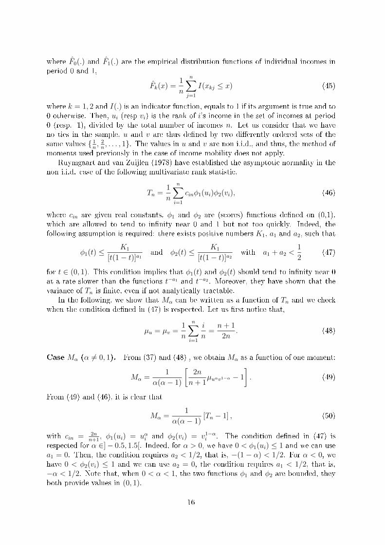
where F0(.) and F1(.) are the empirical distribution functions of individual incomes inperiod 0 and 1,
Fk(x) =1
n
n∑j=1
I(xkj ≤ x) (45)
where k = 1, 2 and I(.) is an indicator function, equals to 1 if its argument is true and to0 otherwise. Then, ui (resp vi) is the rank of i's income in the set of incomes at period0 (resp. 1), divided by the total number of incomes n. Let us consider that we haveno ties in the sample, u and v are thus de�ned by two di�erently ordered sets of thesame values { 1
n, 2n, . . . , 1}. The values in u and v are non i.i.d., and thus, the method of
moments used previously in the case of income mobility does not apply.Ruymgaart and van Zuijlen (1978) have established the asymptotic normality in the
non i.i.d. case of the following multivariate rank statistic,
Tn =1
n
n∑i=1
cinφ1(ui)φ2(vi), (46)
where cin are given real constants, φ1 and φ2 are (scores) functions de�ned on (0,1),which are allowed to tend to in�nity near 0 and 1 but not too quickly. Indeed, thefollowing assumption is required: there exists positive numbers K1, a1 and a2, such that
φ1(t) ≤K1
[t(1− t)]a1and φ2(t) ≤
K1
[t(1− t)]a2with a1 + a2 <
1
2(47)
for t ∈ (0, 1). This condition implies that φ1(t) and φ2(t) should tend to in�nity near 0at a rate slower than the functions t−a1 and t−a2 . Moreover, they have shown that thevariance of Tn is �nite, even if not analytically tractable.
In the following, we show that Mα can be written as a function of Tn and we checkwhen the condition de�ned in (47) is respected. Let us �rst notice that,
µu = µv =1
n
n∑i=1
i
n=n+ 1
2n. (48)
Case Mα (α 6= 0, 1). From (37) and (48) , we obtainMα as a function of one moment:
Mα =1
α(α− 1)
[2n
n+ 1µuαv1−α − 1
]. (49)
From (49) and (46), it is clear that
Mα =1
α(α− 1)[Tn − 1] , (50)
with cin = 2nn+1
, φ1(ui) = uαi and φ2(vi) = v1−αi . The condition de�ned in (47) isrespected for α ∈]− 0.5, 1.5[. Indeed, for α > 0, we have 0 < φ1(ui) ≤ 1 and we can usea1 = 0. Then, the condition requires a2 < 1/2, that is, −(1− α) < 1/2. For α < 0, wehave 0 < φ2(vi) ≤ 1 and we can use a2 = 0, the condition requires a1 < 1/2, that is,−α < 1/2. Note that, when 0 < α < 1, the two functions φ1 and φ2 are bounded, theyboth provide values in (0, 1).
16
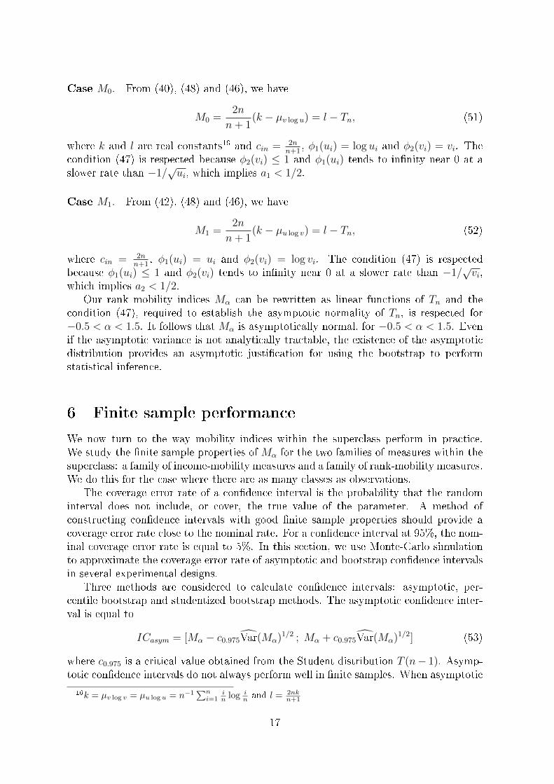
Case M0. From (40), (48) and (46), we have
M0 =2n
n+ 1(k − µv log u) = l − Tn, (51)
where k and l are real constants16 and cin = 2nn+1
, φ1(ui) = log ui and φ2(vi) = vi. Thecondition (47) is respected because φ2(vi) ≤ 1 and φ1(ui) tends to in�nity near 0 at aslower rate than −1/
√ui, which implies a1 < 1/2.
Case M1. From (42), (48) and (46), we have
M1 =2n
n+ 1(k − µu log v) = l − Tn, (52)
where cin = 2nn+1
, φ1(ui) = ui and φ2(vi) = log vi. The condition (47) is respectedbecause φ1(ui) ≤ 1 and φ2(vi) tends to in�nity near 0 at a slower rate than −1/
√vi,
which implies a2 < 1/2.Our rank mobility indices Mα can be rewritten as linear functions of Tn and the
condition (47), required to establish the asymptotic normality of Tn, is respected for−0.5 < α < 1.5. It follows that Mα is asymptotically normal, for −0.5 < α < 1.5. Evenif the asymptotic variance is not analytically tractable, the existence of the asymptoticdistribution provides an asymptotic justi�cation for using the bootstrap to performstatistical inference.
6 Finite sample performance
We now turn to the way mobility indices within the superclass perform in practice.We study the �nite sample properties of Mα for the two families of measures within thesuperclass: a family of income-mobility measures and a family of rank-mobility measures.We do this for the case where there are as many classes as observations.
The coverage error rate of a con�dence interval is the probability that the randominterval does not include, or cover, the true value of the parameter. A method ofconstructing con�dence intervals with good �nite sample properties should provide acoverage error rate close to the nominal rate. For a con�dence interval at 95%, the nom-inal coverage error rate is equal to 5%. In this section, we use Monte-Carlo simulationto approximate the coverage error rate of asymptotic and bootstrap con�dence intervalsin several experimental designs.
Three methods are considered to calculate con�dence intervals: asymptotic, per-centile bootstrap and studentized bootstrap methods. The asymptotic con�dence inter-val is equal to
ICasym = [Mα − c0.975Var(Mα)1/2 ; Mα + c0.975Var(Mα)1/2] (53)
where c0.975 is a critical value obtained from the Student distribution T (n− 1). Asymp-totic con�dence intervals do not always perform well in �nite samples. When asymptotic
16k = µv log v = µu log u = n−1∑ni=1
in log i
n and l = 2nkn+1
17

con�dence intervals give poor coverage, bootstrap con�dence intervals can be expectedto perform better. A variety of bootstrap intervals can be used - for a comprehensive dis-cussion, see Davison and Hinkley (1997). A �rst method, called the percentile bootstrapmethod, does not require the computation and the use of the (asymptotic) standard er-ror of the mobility measure estimated. We generate B bootstrap samples, by resamplingin the original data, and then, for each resample, we compute the mobility index. Weobtain B bootstrap statistics, M b
α, b = 1, . . . , B. The percentile bootstrap con�denceinterval is equal to
ICperc = [cb0.025 ; cb0.975] (54)
where cb0.025 and cb0.975 are the 2.5 and 97.5 percentiles of the EDF of the bootstrapstatistics. A second method, called the studentized bootstrap method, makes use of theasymptotic standard error of the mobility measure estimated. We generate B bootstrapsamples, by resampling in the original data, and then, for each resample, we compute a t-statistic. We obtain B bootstrap t-statistics tbα = (M b
α−Mα)/Var(M bα)1/2, b = 1, . . . , B,
where Mα is the mobility index computed with the original data. The studentizedbootstrap con�dence interval is equal to
ICstud = [Mα − c∗0.975Var(Mα)1/2 ; Mα − c∗0.025Var(Mα)1/2] (55)
where c∗0.025 and c∗0.975 are the 2.5 and 97.5 percentiles of the EDF of the bootstrap t-statistics. It is also called a bootstrap-t or a percentile-t con�dence interval. The maindi�erence between the two bootstrap methods is that the studentized bootstrap con�-dence interval is based on an asymptotically pivotal statistic, not the percentile bootstrapcon�dence interval. Indeed, the t-statistics follow asymptotically a known distribution,which does not depend on unknown parameters. This property is known to providesuperior statistical performance of the bootstrap over asymptotic con�dence intervals(Beran 1987). Note that both bootstrap con�dence intervals are asymmetric. Then,they should provide more accurate con�dence intervals than the asymptotic con�denceinterval when the exact distribution of the statistic is not symmetric. For well-knownreasons - see Davison and Hinkley (1997) or Davidson and MacKinnon (2000) - thenumber of bootstrap resamples B should be chosen so that (B + 1)/100 is an integer.In what follows, we set B = 199.
In our experiments, samples are drawn from a Bivariate Lognormal distribution withparameters
(x0, x1) ∼ LN(µ,Σ) with µ = (0, 0) and Σ =
(1 ρρ 1
)(56)
where µ and Σ are the mean and the square root of the covariance matrix of the vari-able's natural logarithm. The case ρ = 1 corresponds to zero mobility and the caseρ = 0 corresponds to incomes in periods 0 and 1 (resp. x0 and x1) being indepen-dently generated. Then mobility should increases as ρ decreases. The asymptotic dis-tribution is unde�ned for the case of zero mobility (ρ = 1); it is thus interesting tostudy the statistical properties in case of �nearly� zero mobility (ρ = 0.99). In theexperiments, we consider di�erent mobility indices (α = −1,−0.5, 0, 0.5, 1, 1.5, 2), dif-ferent sample sizes (n = 100, 200, 500, 1 000, 5 000, 10 000) and di�erent mobility levels(ρ = 0, 0.2, 0.4, 0.6, 0.8, 0.9, 0.99).
18

For �xed values of α, n and ρ, we draw 10 000 samples from the bivariate lognormaldistribution. For each sample we compute Mα and its con�dence interval at 95%. Thecoverage error rate is computed as the proportion of times the true value of the mobilityindex is not included in the con�dence intervals. The true value of the mobility indexis approximated from a sample of a million observations. Con�dence intervals performwell in �nite sample if the coverage error rate is close to the nominal value, that is, closeto the value 0.05.
6.1 Income mobility
Let us consider the distribution-independent, static status, as de�ned in (36). Here theincome values are used to evaluate individual status: this corresponds to a model ofmovement of incomes.
α -1 0 0.5 1 2
n = 100, ρ = 0 0.3686 0.1329 0.1092 0.1357 0.3730n = 100, ρ = 0.2 0.3160 0.1334 0.1136 0.1325 0.3194n = 100, ρ = 0.4 0.2664 0.1353 0.1221 0.1351 0.2889n = 100, ρ = 0.6 0.2175 0.1346 0.1275 0.1361 0.2263n = 100, ρ = 0.8 0.1718 0.1349 0.1304 0.1345 0.1753n = 100, ρ = 0.9 0.1528 0.1321 0.1308 0.1329 0.1531n = 100, ρ = 0.99 0.1355 0.1340 0.1331 0.1324 0.1333n = 200, ρ = 0 0.3351 0.1077 0.0923 0.1107 0.3153n = 500, ρ = 0 0.2594 0.0830 0.0696 0.0818 0.2631n = 1000, ρ = 0 0.2164 0.0703 0.0609 0.0726 0.2181n = 5000, ρ = 0 0.1713 0.0554 0.0469 0.0522 0.2066n = 10000, ρ = 0 0.1115 0.0532 0.0527 0.0534 0.1151
Table 2: Coverage error rate of asymptotic con�dence intervals at 95% of income mobilitymeasures. The nominal error rate is 0.05, 10.000 replications
Table 2 shows coverage error rates of asymptotic con�dence intervals at 95%. If theasymptotic distribution is a good approximation of the exact distribution of the statistic,the coverage error rate should be close to the nominal error rate, 0.05. From Table 2,we can see that:
• asymptotic con�dence intervals always perform poorly for α = −1, 2,
• the coverage error rate is stable as ρ varies (for α = 0, 0.5, 1 and n = 100),
• the coverage error rate decreases as n increases,
• the coverage error rate is close to 0.05 for n ≥ 5.000 and α = 0, 0.5, 1.
These results suggest that asymptotic con�dence intervals perform well in very largesample, with α ∈ [0, 1].
19
α -1 0 0.5 1 2
n = 100, ρ = 0.8Asymptotic 0.1718 0.1349 0.1304 0.1345 0.1753Boot-perc 0.1591 0.1294 0.1215 0.1266 0.1552Boot-stud 0.0931 0.0751 0.0732 0.076 0.0952n = 200, ρ = 0.8Asymptotic 0.1315 0.0973 0.0927 0.0973 0.1276Boot-perc 0.1222 0.0943 0.0900 0.0950 0.1176Boot-stud 0.0794 0.0666 0.0660 0.0688 0.0791n = 500, ρ = 0.8Asymptotic 0.1127 0.0847 0.0828 0.0857 0.1124Boot-perc 0.1054 0.0814 0.0813 0.0843 0.1036Boot-stud 0.0765 0.0641 0.0629 0.0630 0.0779n = 1.000, ρ = 0.8Asymptotic 0.0880 0.0678 0.0659 0.0672 0.0864Boot-perc 0.0862 0.0672 0.0661 0.0689 0.0851Boot-stud 0.0680 0.0585 0.0589 0.0596 0.0693
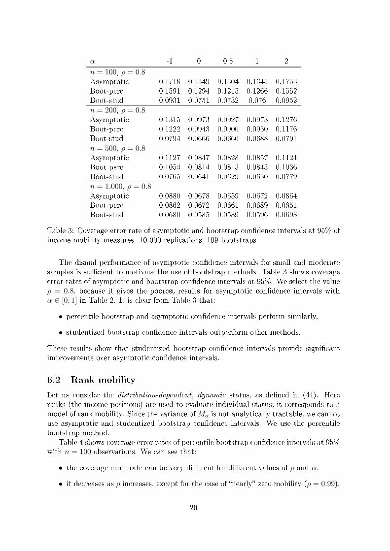
Table 3: Coverage error rate of asymptotic and bootstrap con�dence intervals at 95% ofincome mobility measures. 10 000 replications, 199 bootstraps
The dismal performance of asymptotic con�dence intervals for small and moderatesamples is su�cient to motivate the use of bootstrap methods. Table 3 shows coverageerror rates of asymptotic and bootstrap con�dence intervals at 95%. We select the valueρ = 0.8, because it gives the poorest results for asymptotic con�dence intervals withα ∈ [0, 1] in Table 2. It is clear from Table 3 that:
• percentile bootstrap and asymptotic con�dence intervals perform similarly,
• studentized bootstrap con�dence intervals outperform other methods,
These results show that studentized bootstrap con�dence intervals provide signi�cantimprovements over asymptotic con�dence intervals.
6.2 Rank mobility
Let us consider the distribution-dependent, dynamic status, as de�ned in (44). Hereranks (the income positions) are used to evaluate individual status; it corresponds to amodel of rank mobility. Since the variance ofMα is not analytically tractable, we cannotuse asymptotic and studentized bootstrap con�dence intervals. We use the percentilebootstrap method.
Table 4 shows coverage error rates of percentile bootstrap con�dence intervals at 95%with n = 100 observations. We can see that:
• the coverage error rate can be very di�erent for di�erent values of ρ and α,
• it decreases as ρ increases, except for the case of �nearly� zero mobility (ρ = 0.99).
20

α -0.5 0 0.5 1 1.5
ρ = 0 0.5592 0.1575 0.1088 0.1583 0.5282ρ = 0.2 0.3176 0.1122 0.0884 0.1135 0.3231ρ = 0.4 0.1883 0.0931 0.0755 0.0913 0.1876ρ = 0.6 0.1122 0.0767 0.0651 0.0741 0.1118ρ = 0.8 0.0671 0.0593 0.0555 0.0590 0.0652ρ = 0.9 0.0432 0.0430 0.0431 0.0441 0.0446ρ = 0.99 0.0983 0.0985 0.0981 0.0984 0.0992
Table 4: Coverage error rate of percentile bootstrap con�dence intervals at 95% of rank-mobility measures. 10 000 replications, 199 bootstraps and 100 observations.
α -0.5 0 0.5 1 1.5
n = 100, ρ = 0 0.5592 0.1575 0.1088 0.1583 0.5282n = 200 0.4613 0.1143 0.0833 0.1180 0.4723n = 500 0.3548 0.0868 0.0645 0.0814 0.3644n = 1000 0.3135 0.0672 0.0556 0.0735 0.3170n = 100, ρ = 0.9 0.0432 0.0430 0.0431 0.0441 0.0446n = 200 0.0454 0.0441 0.0456 0.0454 0.0459n = 500 0.0500 0.0499 0.0485 0.0480 0.0483n = 1000 0.0511 0.0509 0.0539 0.0538 0.0538n = 100, ρ = 0.99 0.0983 0.0985 0.0981 0.0984 0.0992n = 200 0.0981 0.0971 0.0970 0.0974 0.0977n = 500 0.0855 0.0838 0.0833 0.0822 0.083n = 1000 0.0788 0.0777 0.0762 0.0767 0.0771
Table 5: Coverage error rate of percentile bootstrap con�dence intervals at 95% of rank-mobility measures. 10 000 replications, 199 bootstraps.
• the coverage error rate is close to 0.05 for ρ = 0.8, 0.9 and α = 0, 0.5, 1.
These results suggest that percentile bootstrap con�dence intervals perform well in smallsample in the presence of low but signi�cant mobility levels (ρ = 0.8, 0.9) and for α ∈[0, 1].
Table 5 shows coverage error rates of percentile bootstrap con�dence intervals at 95%as the sample size increases. We can see that:
• the coverage error rate gets closer to 0.05 as the sample size increases,
• the coverage error rate is smaller when α = 0, 0.5, 1.
These results show that percentile bootstrap con�dence intervals have better statisticalproperties as the sample size increases.
21
7 Conclusion
What makes our approach to mobility measurement novel is not the introduction of anew speci�c index but rather a way of rethinking the representation of the problem andthen the theoretical and statistical treatment of this representation of mobility. The keystep involves a logical separation of fundamental concepts, (1) the measure of individualstatus and (2) the aggregation of changes in status.
The status concept is derived directly from information available in the marginaldistributions. It could involve the simplest derivation - the assumption that statusequals income. Or it could involve something more sophisticated, incorporating theperson's location in the income distribution. This is a matter for normative judgment.
The aggregation of changes in status involves the application of standard principles tostatus pairs. From this one derives a superclass of mobility measures - a class of classesof measures. As we have seen this is generally applicable to a wide variety of statusconcepts and, for any given status concept, the members of the class are indexed by aparameter α that determines the type of mobility measure. Each measure in each class ofthe superclass involves a kind of averaging of individual mobilities and the evaluation ofindividual mobility depends on status in the two periods, but no more (in our approachrank may be important for status but not for quantifying movement). Every measurein the superclass has attractive scale properties that imply structural regularity, but nomore than that; once again this is because status can be separated from - if not divorcedfrom - income and wealth.
We have also shown that the principal status types that are likely to be adoptedin practice will result in statistically tractable mobility indices. Bootstrap con�denceintervals perform well in moderate sample sizes for α in the interval [0, 1], in the casesof both income mobility and rank mobility.
22

References
Aczél, J. (1966). Lectures on Functional Equations and their Applications. Number 9in Mathematics in Science and Engineering. New York: Academic Press.
Aczél, J. and J. G. Dhombres (1989). Functional Equations in Several Variables. Cam-bridge: Cambridge University Press.
Atkinson, A. B. (1981). On intergenerational income mobility in Britain. Journal ofPost Keynesian Economics 3, 194�218.
Atkinson, A. B. (1983). The measurement of economic mobility. In A. B. Atkinson(Ed.), Social Justice and Public Policy, Chapter 3, pp. 61�75. Hemel Hempstead,UK.: Harvester Wheatsheaf.
Atkinson, A. B. and F. Bourguignon (1982). The comparison of multi-dimensionaldistributions of economic status. Review of Economic Studies 49, 183�201.
Atoda, N. and T. Tachibanaki (1991). Earnings distribution and inequality over time:Education versus relative position and cohort. International Economic Review 32,475�489.
Ayala, L. and M. Sastre (2008). The structure of income mobility: empirical evidencefrom �ve UE countries. Empirical Economics 35, 451�473.
Bénabou, R. and E. A. Ok (2001). Mobility as progressivity: Ranking income processesaccording to equality of opportunity. NBER Working Paper W8431, National Bu-reau of Economic Research.
Beran, R. (1987). Prepivoting to reduce level error of con�dence sets. Biometrika 74,457�468.
Bibby, J. (1975). Methods of measuring mobility. Quality and Quantity 9, 107�136.
Bossert, W. and A. P�ngsten (1990). Intermediate inequality: concepts, indices andwelfare implications. Mathematical Social Science 19, 117�134.
Chakravarty, S. R. (1984). Normative indices for measuring social mobility. EconomicsLetters 15, 175�180.
Chakravarty, S. R., B. Dutta, and J. Weymark (1985). Ethical indices of incomemobility. Social Choice and Welfare 2, 1�21.
Cowell, F. A. (1985). Measures of distributional change: An axiomatic approach.Review of Economic Studies 52, 135�151.
D'Agostino, M. and V. Dardanoni (2009). The measurement of rank mobility. Journalof Economic Theory 144, 1783�1803.
Dardanoni, V. (1993). Measuring social mobility. Journal of Economic Theory 61,372�394.
Davidson, R. and J. G. MacKinnon (2000). Bootstrap tests: How many bootstraps?Econometric Reviews 19, 55�68.
23

Davison, A. C. and D. V. Hinkley (1997). Bootstrap Methods. Cambridge: CambridgeUniversity Press.
Demuynck, T. and D. Van de gaer (2010, January). Rank dependent relative mobilitymeasures. Working Papers of Faculty of Economics and Business Administration,Ghent University, Belgium 10/628, Ghent University, Faculty of Economics andBusiness Administration.
Eichhorn, W. (1978). Functional Equations in Economics. Reading Massachusetts:Addison Wesley.
Eichhorn, W. (1988). On a class of inequality measures. Social Choice and Welfare 5,171�177.
Fields, G. S. and E. A. Ok (1996). The meaning and measurement of income mobility.Journal of Economic Theory 71 (2), 349�377.
Fields, G. S. and E. A. Ok (1999a). The measurement of income mobility: an in-troduction to the literature. In J. Silber (Ed.), Handbook on Income InequalityMeasurement. Dewenter: Kluwer.
Fields, G. S. and E. A. Ok (1999b). Measuring movement of incomes. Economica 66,455�472.
Fishburn, P. C. (1970). Utility Theory for Decision Making. New York: John Wiley.
Gottschalk, P. and E. Spolaore (2002). On the evaluation of economic mobility. Reviewof Economic Studies 69, 191�208.
Kearl, J. R. and C. L. Pope (1984). Mobility and distribution. Review of Economicsand Statistics 66, 192�199.
King, M. A. (1983). An index of inequality: with applications to horizontal equityand social mobility. Econometrica 51, 99�116.
Markandya, A. (1982). Intergenerational exchange mobility and economic welfare.European Economic Review 17, 301�324.
Markandya, A. (1984). The welfare measurement of changes in economic mobility.Economica 51, 457�471.
Mitra, T. and E. A. Ok (1998). The measurement of income mobility: A partialordering approach. Economic Theory 12, 77�102.
Ruiz-Castillo, J. (2004). The measurement of structural and exchange income mobility.Journal of Economic Inequality 2, 219�228.
Ruymgaart, F. H. and M. C. A. van Zuijlen (1978). Asymptotic normality of multi-variate linear rank statistics in the non-i.i.d. case. Annals of Statistics 6, 588�602.
Schluter, C. and D. Van de gaer (2011). Structural mobility, exchange mobility andsubgroup consistent mobility measurement, US - German mobility rankings revis-ited. Review of Income and Wealth forthcoming.
Shorrocks, A. F. (1978). The measurement of mobility. Econometrica 46, 1013�1024.
Tsui, K. (2009). Measurement of income mobility: A re-examination. Social Choiceand Welfare 33, 629�645.
24

Van de gaer, D., E. Schokkaert, and M. Martinez (2001). Three meanings of intergen-erational mobility. Economica 68, 519�537.
Van Kerm, P. (2004). What lies behind income mobility? Reranking and distributionalchange in Belgium, Western Germany and the USA. Economica 71, 223�239.
Van Kerm, P. (2009). Income mobility pro�les. Economics Letters 102, 93�95.
25

A Proofs
Proof. [Proof of Theorem 1] . Axioms 1 to 4 imply that � can be represented by acontinuous function Φ : Zn → R that is increasing in |ui − vi|, i = 1, ..., n. Using Axiom3 part (a) of the result follows from Theorem 5.3 of Fishburn (1970). Now take z′ andz in as speci�ed in Axiom 4. Using (11) it is clear that z ∼ z′ if and only if
φi (ui + δ, ui + δ)− φi (ui, ui)− φj (uj + δ, uj + δ) + φj (uj + δ, uj + δ) = 0
which can only be true if
φi (ui + δ, ui + δ)− φi (ui, ui) = f (δ)
for arbitrary ui and δ. This is a standard Pexider equation and its solution implies (12).
Proof. [Proof of Theorem 2] Using the function Φ introduced in the proof of Theorem1 Axiom 5 implies
Φ (z) = Φ (z′)
Φ (tz) = Φ (tz′)
and so, since this has to be true for arbitrary z, z′ we have
Φ (tz)
Φ (z)=
Φ (tz′)
Φ (z′)= ψ (t)
where ψ is a continuous function R→ R. Hence, using the φi given in (11), we have forall z:
φi (tzi) = ψ (t)φi (zi) i = 1, ..., n.
or, equivalentlyφi (tui, tvi) = ψ (t)φi (ui, vi) , i = 1, ..., n. (57)
So, in view of Aczél and Dhombres (1989), page 346 there must exist c ∈ R and afunction Hi : R+ → R such that
φi (ui, vi) = uciHi
(uivi
). (58)
From (12) and (58) it is clear that
φi (ui, ui) = uciHi (1) = ai + biui, (59)
which implies c = 1. Putting (58) with c = 1 into (13) gives the result.
Proof. [Proof of Theorem 3] Take the special case where, in distribution z′0 theindividual movement takes the same value r for all n. If (ui, vi) represents a typicalcomponent in z0 then z0∼ z′0 implies
r = ψ
(n∑i=1
uiHi
(uivi
))(60)
26

where ψ is the solution in r to
n∑i=1
uiHi
(uivi
)=
n∑i=1
uiHi (r) (61)
In (61) can take the ui as �xed weights. Using Axiom 6 in (60) requires
tr = ψ
(n∑i=1
uiHi
(tuivi
)), for all t > 0. (62)
Using (61) we have
n∑i=1
uiHi
(tψ
(n∑i=1
uiHi
(uivi
)))=
n∑i=1
uiHi
(tuivi
)(63)
Introduce the following change of variables
ui := uiHi
(uivi
), i = 1, ..., n (64)
and write the inverse of this relationship as
uivi
= ψi (ui) , i = 1, ..., n (65)
Substituting (64) and (65) into (63) we get
n∑i=1
uiHi
(tψ
(n∑i=1
ui
))=
n∑i=1
uiHi (tψi (ui)) . (66)
Also de�ne the following functions
θ0 (u, t) :=n∑i=1
uiHi (tψ (u)) (67)
θi (u, t) := uiHi (tψi (u)) , i = 1, ..., n. (68)
Substituting (67),(68) into (66) we get the Pexider functional equation
θ0
(n∑i=1
ui, t
)=
n∑i=1
θi (ui, t)
which has as a solution
θi (u, t) = bi (t) +B (t)u, i = 0, 1, ..., n
where
b0 (t) =n∑i=1
bi (t)
27
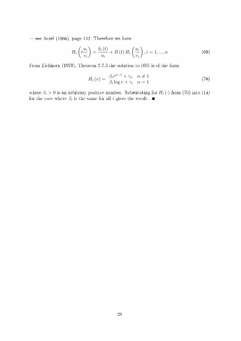
� see Aczél (1966), page 142. Therefore we have
Hi
(tuivi
)=bi (t)
ui+B (t)Hi
(uivi
), i = 1, ..., n (69)
From Eichhorn (1978), Theorem 2.7.3 the solution to (69) is of the form
Hi (v) =βiv
α−1 + γi, α 6= 1βi log v + γi α = 1
(70)
where βi > 0 is an arbitrary positive number. Substituting for Hi (·) from (70) into (14)for the case where βi is the same for all i gives the result.
28