ESTIMATION AND CONTROL OF NONLINEAR SYSTEMS USING EXTENDEDHIGH-GAIN OBSERVERS

By

Almuatazbellah Muftah Boker

A DISSERTATION

Submitted toMichigan State University

in partial fulfillment of the requirementsfor the degree of

Electrical Engineering - Doctor of Philosophy

2013

ABSTRACT

ESTIMATION AND CONTROL OF NONLINEAR SYSTEMS USING EXTENDEDHIGH-GAIN OBSERVERS

By

Almuatazbellah Muftah Boker

Providing accurate state estimation is important for many systems. This is especially the case for

systems whose states may be very difficult or even impossible to measure or require expensive or

unreliable sensors. From another prospective, making all the states available simplifies consider-

ably the control design and helps in providing practical and economic solutions to many control

problems. The first part of our work involves the design of an observer for a class of nonlinear

systems that can potentially admit unstable zero dynamics. The structure of the observer is com-

posed of an Extended High-Gain Observer (EHGO), for the estimation of the derivatives of the

output, augmented with an Extended Kalman Filter for the estimation of the states of the internal

dynamics. The EHGO is also utilized to estimate a signal that is used as a virtual output to an

auxiliary system comprised of the internal dynamics. We demonstrate the efficacy of the observer

in two examples; namely, a synchronous generator connected to an infinite bus and a Translating

Oscillator with a Rotating Actuator (TORA) system.

In the special case of the system being linear in the states of the internal dynamics, we achieve

semi-global asymptotic convergence of the estimation error. We also solve for this class of sys-

tems, which may have unstable zero dynamics, the problem of output feedback stabilization. We

allow the use of any globally stabilizing full state feedback control scheme. We then recover its

performance using an observer-based output feedback control. As a demonstration of the efficacy

of this control scheme, we design an output feedback stabilizing control for the DC-to-DC boost

converter system.

We also consider the problem of output feedback tracking of possibly non-minimum phase

nonlinear systems where the internal dynamics have a full relative degree with respect to a virtual

output. In this case, the internal dynamics can be represented in the chain-of-integrators form. This

allows the use of a high-gain observer to estimate the states of the internal dynamics, and hence,

making all the system states available for the controller. We allow the use of any globally stabiliz-

ing full state feedback control and we show that it is possible to recover its stability properties and

trajectory performance. Finally, as a demonstration of the design procedure, we solve the problem

of output feedback tracking control of flexible joint manipulators where the link angle is the output

to be controlled and the motor angle is the measured output. We demonstrate the effectiveness of

the proposed scheme in the single link case, and where the zero dynamics are not asymptotically

stable.

To my mother Naiema, father Muftah, wife Mona and my kids Jood and Muhammad.

iv

ACKNOWLEDGMENTS

First and foremost, thanks to God for his endless bounties.

This work would not have been possible without the help and guidance of Professor Hassan

Khalil. I am extremely fortunate to have him as my mentor and advisor. His deep understanding of

the subject, patience and hard work have been, and will always be, sources of inspiration for me. I

will always be grateful for his unwavering support and encouragement.

I would also like to thank my other committee members Prof. Tan, Prof. Zhu and Prof. Mukher-

jee for their insightful feedback.

I owe my parents everything. Their unconditional love and support is limitless. My mother’s

love, care and patience is like a guardian accompanying me everywhere. My father’s virtues,

leading by example and love to serve others have always led me to be the best i can be.

Last but not least, this journey would have been really difficult without the support and love of

my friend, partner and wife Mona. I also would like to thank her for being a fabulous mom for our

two beloved children Jood and Muhammad.

v

TABLE OF CONTENTS

LIST OF FIGURES . . . . . . . . . . . . . . . . . . . . . . . . . . . . . . . . . . . . . . viii

Chapter 1 Introduction . . . . . . . . . . . . . . . . . . . . . . . . . . . . . . . . . . 11.1 Nonlinear Observers . . . . . . . . . . . . . . . . . . . . . . . . . . . . . . . . . 1

1.1.1 High-Gain and Extended High-Gain Observers: Brief Background . . . . . 21.2 Non-minimum Phase Nonlinear Systems . . . . . . . . . . . . . . . . . . . . . . . 6

1.2.1 Observers for Non-minimum Phase Nonlinear System . . . . . . . . . . . 61.2.2 Output Feedback Control of Non-minimum Phase Nonlinear Systems . . . 6

1.3 Importance and Motivations . . . . . . . . . . . . . . . . . . . . . . . . . . . . . 81.4 An Overview of the Dissertation . . . . . . . . . . . . . . . . . . . . . . . . . . . 9

Chapter 2 Nonlinear Observers Comprising High-Gain Observers and ExtendedKalman Filters . . . . . . . . . . . . . . . . . . . . . . . . . . . . . . . . . 10

2.1 Introduction . . . . . . . . . . . . . . . . . . . . . . . . . . . . . . . . . . . . . . 102.2 Problem formulation . . . . . . . . . . . . . . . . . . . . . . . . . . . . . . . . . 122.3 Linear Systems . . . . . . . . . . . . . . . . . . . . . . . . . . . . . . . . . . . . 132.4 General case . . . . . . . . . . . . . . . . . . . . . . . . . . . . . . . . . . . . . . 15

2.4.1 Observer Design For a Synchronous Generator Connected to an InfiniteBus System . . . . . . . . . . . . . . . . . . . . . . . . . . . . . . . . . . 25

2.5 Special case: System linear in the internal state η . . . . . . . . . . . . . . . . . . 272.5.1 Observer Design For The Translating Oscillator With a Rotating Actuator

System . . . . . . . . . . . . . . . . . . . . . . . . . . . . . . . . . . . . 302.6 Conclusions . . . . . . . . . . . . . . . . . . . . . . . . . . . . . . . . . . . . . . 34

Chapter 3 Output Feedback Stabilization of Possibly Non-Minimum Phase Nonlin-ear Systems . . . . . . . . . . . . . . . . . . . . . . . . . . . . . . . . . . . 35

3.1 Introduction . . . . . . . . . . . . . . . . . . . . . . . . . . . . . . . . . . . . . . 353.2 Problem Formulation . . . . . . . . . . . . . . . . . . . . . . . . . . . . . . . . . 373.3 State Feedback . . . . . . . . . . . . . . . . . . . . . . . . . . . . . . . . . . . . 383.4 Output Feedback . . . . . . . . . . . . . . . . . . . . . . . . . . . . . . . . . . . 39

3.4.1 Stability Recovery . . . . . . . . . . . . . . . . . . . . . . . . . . . . . . 443.4.2 Trajectory Recovery . . . . . . . . . . . . . . . . . . . . . . . . . . . . . 49

3.5 Output Feedback Control of a DC-to-DC Boost Converter System . . . . . . . . . 563.6 Conclusions . . . . . . . . . . . . . . . . . . . . . . . . . . . . . . . . . . . . . . 61

Chapter 4 Control of Nonlinear Systems Using Full-Order High Gain Observers:A Separation Principle Approach . . . . . . . . . . . . . . . . . . . . . . 62

4.1 Introduction . . . . . . . . . . . . . . . . . . . . . . . . . . . . . . . . . . . . . . 62

vi

4.2 Motivating Example: Tracking Control of Flexible Joint Manipulators Using OnlyMotor Position Feedback . . . . . . . . . . . . . . . . . . . . . . . . . . . . . . . 644.2.1 Problem Formulation . . . . . . . . . . . . . . . . . . . . . . . . . . . . . 664.2.2 Full-State Feedback Control . . . . . . . . . . . . . . . . . . . . . . . . . 674.2.3 Output Feedback Control . . . . . . . . . . . . . . . . . . . . . . . . . . . 694.2.4 Simulation Example: Single-Link Flexible Joint Manipulators . . . . . . . 70

4.2.4.1 Case 1: without parameter uncertainties . . . . . . . . . . . . . . 734.2.4.2 Case 2: with parameter uncertainties . . . . . . . . . . . . . . . 764.2.4.3 Discussion . . . . . . . . . . . . . . . . . . . . . . . . . . . . . 78

4.3 General Formulation . . . . . . . . . . . . . . . . . . . . . . . . . . . . . . . . . 804.4 Full State Feedback Control . . . . . . . . . . . . . . . . . . . . . . . . . . . . . . 824.5 Observer Design . . . . . . . . . . . . . . . . . . . . . . . . . . . . . . . . . . . . 844.6 Output Feedback Control . . . . . . . . . . . . . . . . . . . . . . . . . . . . . . . 864.7 Conclusions . . . . . . . . . . . . . . . . . . . . . . . . . . . . . . . . . . . . . . 99

Chapter 5 Conclusions and Future Work . . . . . . . . . . . . . . . . . . . . . . . . 1005.1 Concluding Remarks . . . . . . . . . . . . . . . . . . . . . . . . . . . . . . . . . 1005.2 Future Work . . . . . . . . . . . . . . . . . . . . . . . . . . . . . . . . . . . . . . 103

BIBLIOGRAPHY . . . . . . . . . . . . . . . . . . . . . . . . . . . . . . . . . 105

vii

LIST OF FIGURES

Figure 2.1 Estimation of the states η1 and η2. For interpretation of the references tocolor in this and all other figures, the reader is referred to the electronicversion of this dissertation. . . . . . . . . . . . . . . . . . . . . . . . . . 26

Figure 2.2 Estimation error of the signal σ . . . . . . . . . . . . . . . . . . . . . . . 27

Figure 2.3 Estimation of the state θ . . . . . . . . . . . . . . . . . . . . . . . . . . . 33

Figure 2.4 Estimation of the internal states xc and xc. . . . . . . . . . . . . . . . . . 33

Figure 3.1 Output response. . . . . . . . . . . . . . . . . . . . . . . . . . . . . . . . 58

Figure 3.2 Estimation error (η− η). . . . . . . . . . . . . . . . . . . . . . . . . . . 59

Figure 3.3 Control effort. . . . . . . . . . . . . . . . . . . . . . . . . . . . . . . . . 60

Figure 3.4 Recovery of the state of the auxiliary system. . . . . . . . . . . . . . . . 60

Figure 4.1 Tracking of the link angle to a reference signal. . . . . . . . . . . . . . . 74

Figure 4.2 Control Effort. . . . . . . . . . . . . . . . . . . . . . . . . . . . . . . . . 74

Figure 4.3 Recovery of the state feedback performance. . . . . . . . . . . . . . . . . 75

Figure 4.4 Tracking and estimation errors of the state η1 in the presence of noise. . . 76

Figure 4.5 Tracking error and estimation error in the case of uncertain load mass M. . 77

Figure 4.6 Tracking error and estimation error in the case of uncertain joint stiffness k. 78

viii

Chapter 1

Introduction

1.1 Nonlinear Observers

While the literature on linear observer theory may have reached a saturation point, research on

observers for nonlinear systems is far from complete. In fact, a unified approach to observer design

for nonlinear systems still seems to be hard to formulate. In addition, one of the difficult properties

to achieve in this context is the arbitrary enlargement of the region of attraction of the observer

stability. In general, there have been a number of different approaches to this problem. The first

approach is based on the extension of the Leunberger observers [1] and Kalman filters [2], [3] to

nonlinear systems. This approach is based on linearization and is appealing due to the simplicity

of the observer design regardless of the complexity of the system. However, the drawback of

this approach is that it guarantees only local stability. Section 2.1 of this dissertation will have

more discussion on the use of Kalman filters in the estimation of nonlinear systems. The second

approach utilizes the idea of linearizing the error dynamics, by the use of state transformation, so

that the nonlinearities may only depend on the inputs and outputs, see e.g. [4], [5], [6]. The third

approach is based on the use of Linear Matrix Inequalities (LMI) techniques, see e.g. [7], [8],

[9]. The systems considered by this approach are composed of a linear part and a nonlinear part

that satisfies some monotonic properties. The feasibility of this approach is closely linked to the

feasibility of the solution of the LMI. The fourth main approach is based on the use of high-gain

1

observers [10] and sliding mode observers [11]. These observers deal with systems that are in the

uniformly observable normal form, where the nonlinearities appear in a lower triangular structure.

This approach has gained popularity due to its robustness properties. The above approaches are by

no means exclusive and, in fact, there have been results that make use of techniques from different

approaches. Just to give an example, the paper by [12] merges the techniques of the extended

Kalman filter and high-gain observer to solve the problem of state estimation for systems in the

normal form with stable linear internal dynamics. It should also be mentioned that there have been

other results that may not fall into the above approaches such as [13], [14], [15].

1.1.1 High-Gain and Extended High-Gain Observers: Brief Background

High-gain observers constitute a key part in the work presented in this dissertation. Therefore,

we will start by giving a brief background about their design. Consider the following third order

system

x1 = x2 (1.1)

x2 = f1(x1,x2,x3)+u (1.2)

x3 = x1 + x2− x3 (1.3)

y = x1 (1.4)

where x ∈ R3 is the state vector, u is the control input and y is the output. We assume that the

function f1 satisfies f1(0,0,x3) = 0 and can be unknown. This system is minimum phase with zero

dynamics x3 =−x3. If we are interested in estimating the state x2 and assuming the presence of a

2

stabilizing control u, we can design the following high-gain observer

˙x1 = x2 +α1

ε(y− x1) (1.5)

˙x2 = f1(x1, x2)+u+α2

ε2 (y− x1) (1.6)

In this case f1(., .) could take any nominal value and can even be set to zero. The observer constants

α1 and α2 are chosen such that the polynomial s2 +α1s+α2 is Hurwitz, and ε > 0 is a small

parameter. This observer can be augmented with an open loop observer to estimate the state x3.

This allows the design of a full information output feedback control.

In general, it can be shown that high-gain observers can provide estimates of the output and

its derivatives, see e.g. [16]. Therefore, it can estimate the right hand side of (1.2), and thus,

can estimate the unknown function f1. In this case, the observer is called an Extended High Gain

Observer (EHGO). To illustrate this idea, let σ = f1(x1,x2,x3), and extend the dimension of (1.1)-

(1.2) by adding σ as an extra state variable as follows

x1 = x2

x2 = σ +u

σ = f2(x1,x2,x3,u)

(1.7)

where

f2 =d f1

dt=

∂ f1

∂x1x2 +

∂ f1

∂x2[ f1(x1,x2,x3)+u]+

∂ f1

∂x3[x1 + x2− x3].

3

Consequently, a high-gain observer for (1.7) can be designed as

˙x1 = x2 +α1

ε(y− x1)

˙x2 = σ +u+α2

ε2 (y− x1)

˙σ = f2(x1, x2, x3,u)+α3

ε3 (y− x1)

(1.8)

and f1 = σ . It is also worth mentioning that the effect of f2 is attenuated as ε→ 0, thus the observer

can tolerate f2 being unknown and achieve an estimation error of the order O(ε).

In general, high-gain observers have proved useful in nonlinear feedback control. The refer-

ence [17] provides a survey of the development of high-gain observers over the past two decades.

Basically, there have been two independent schools of research on this subject. The first school,

lead mostly by French researchers (Gauthier, Hammouri, and others) focused on deriving global

results by considering global Lipschitz conditions; see e.g. [18], [19], [20], [21]. In the context

of output feedback and in the absence of global Lipschitz condition, the second school, lead by

Khalil, realized the destabilizing effect of the peaking phenomenon and proposed a solution for it

[22]. The solution was simply to ensure global boundedness of the control over a region of interest,

which can be done by saturating the state estimates.

High-gain observers have been successfully employed in partial state output feedback stabi-

lization schemes [22], [23], and output tracking using sliding mode control [24]. Previous work on

full order high-gain observers is limited to minimum phase systems. Reference [25], for instance,

proposed a full order observer that employs an open loop observer for the internal dynamics, which

limits the validity of the technique to minimum phase systems. Another paper [12] proposed the

use of an EKF-based high-gain observer for the estimation of the full state vector of minimum

phase systems with linear internal dynamics driven only by the output.

4

Extended high-gain observers have been used in the literature to serve different objectives.

They have been used to provide estimates of unknown signals that represent model uncertainties

or external inputs so that they could be canceled by the controller [26]. Within the framework of

designing a full information state feedback control, similar approach was also used in [27] where

a first order high-gain observer was used to estimate matched uncertainties so are then canceled by

the control. Around the same time, [28] introduced an output feedback control strategy that utilizes

an inner loop control based on the use of high-gain observer to estimate the inverse of a nominal

model of the closed loop behavior of the plant, and an outer loop controller to shape the transient

response. A very important feature that was achieved by [26], [27] and [28] is the ability to recover

desired transient performance by the use of the nonlinear control, despite the presence of matched

model uncertainties and disturbances. Indeed the high-gain observer was instrumental in achieving

this feature. EHGO is also used to develop a Lyapunov-based switching control strategy [29], [30].

More recently, the work in [31] utilizes the EHGO to estimate a signal that is observable to the zero

dynamics of a non-minimum phase system. This allowed the design of a stabilizing controller.

The wide use of high-gain observers in control applications is mainly due to a number of

properties that may not be provided by other observers. The first property is the simplicity of

design, where there is no need for complex gain formulas and solving LMI or partial differential

equations. Secondly, the observer provides the ability to recover the state trajectories when used

in output feedback control. This property is rarely considered in the literature and is very useful

to the designer as it helps in shaping the transient response. Another useful property is the ability

of the high-gain observer to robustly estimate the states in the presence of disturbances or model

uncertainties.

5

1.2 Non-minimum Phase Nonlinear Systems

In recent years, more attention was directed towards the study of non-minimum phase nonlinear

systems. This has been motivated by many reasons, one of them is the fact that unstable zero

dynamics is an intrinsic feature of a wide variety of systems. Examples of these systems include

flexible-joint robotic manipulators, electromechanical systems, under-actuated systems and chem-

ical reactors. The focus on non-minimum phase systems also comes after many advances in the

control of minimum phase systems, such as the success that has been enjoyed by the use of feed-

back linearization techniques.

1.2.1 Observers for Non-minimum Phase Nonlinear System

There have been a few techniques that dealt with observer design for non-minimum phase non-

linear systems and achieved non-local convergence results. For example, a method for designing

observers for systems affine in the unmeasured states was introduced in [32] and for a more general

class of nonlinear systems in [14]. The key idea in these results is the construction of an invariant

and attractive manifold. This has to be achieved by solving a set of partial differential equations.

Reference [33] proposed a Higher Order Sliding Mode Observer to estimate the full state vector

with a vector of unknown inputs for non-minimum phase nonlinear systems. It considered the case

when the internal dynamics are quasilinear and the forcing term can be piece-wise modeled as the

output of a dynamical process given by an unknown linear system with a known order.

1.2.2 Output Feedback Control of Non-minimum Phase Nonlinear Systems

In the linear case the separation principle guarantees the global stabilization by any linear state

feedback control can be achieved by output feedback when the states are replaced by their esti-

6

mates. However, this principle is not valid for nonlinear observer-based output feedback systems.

Furthermore, the results that has been reported in this regard, such as the ones reported in [34],

[35] [36], are not valid for any observer design. One of the observers that satisfies this principle,

nevertheless, is the high-gain observer.

One of the first results on the control of non-minimum phase nonlinear systems is by A. Isidori.

In his paper [37], he proved semi-global stabilization for a general class of non-minimum phase

nonlinear systems assuming the existence of a dynamic stabilizing controller for an auxiliary

system. The same problem was considered in [31], where robust semi-global stabilization was

achieved under similar assumptions but with an extended high-gain observer based output feed-

back controller. This paper showed the potential of using the extended high-gain observer as an

alternative for the high-gain feedback scheme of [37].

Papers [38] and [39] consider a special case of the normal form, called the output feedback

form, where the internal dynamics depend only on the output. Paper [38] allows the presence of

disturbances and paper [39] allows model uncertainty. They both require various stabilizability

conditions on the internal dynamics. Paper [40] also considers systems in the output feedback

form and assumes the system will be minimum phase with respect to a new output, defined as a

linear combination of the state variables. Paper [6] solves the stabilization problem for the output

feedback form with linear zero dynamics. It uses backstepping technique and an observer with

linear error dynamics to achieve semi-global stabilizability result. Another result reported in [41]

deals with a special case of the normal form where the internal dynamics are modeled as a chain

of integrators. This work uses adaptive output feedback controller based on Neural Networks

and a linear state observer to achieve ultimate boundedness of the states in the presence of model

uncertainties. Basically, observer and controller designs are performed for a linearized model of the

system, then, Neural Networks are used to represent modeling uncertainties. Moreover, adaptive

7

laws for the NN and adaptive gains are obtained from using Lyapunov’s direct method.

1.3 Importance and Motivations

In this dissertation, we solve the problem of estimating all the states of nonlinear systems repre-

sented in the normal form. This allows us to solve the problem of output feedback control for the

same class of systems. A key tool that helps in solving this problem is the high-gain observer. As

eluded to in Section 1.1.1, high-gain observers have been mostly used in partial state feedback and

have been limited to minimum phase systems. We, on the other hand, show that by using this tool

we can solve problems where estimates of all the states are needed and the zero dynamics may not

be stable. As a result, the full order observer proposed in this dissertation is characterized by the

simplicity of design relative to what have been offered in the literature. Furthermore, the proposed

observer-based output feedback schemes have the capability to partially recover the trajectories

under state feedback.1 This sets the proposed output feedback scheme apart from others in the

literature.

The motivations of this work can be summarized by the following points

1. Solve the problem of estimation and control of a general class of nonlinear systems. This

class of systems can include non-minimum phase systems. This problem is not widely stud-

ied in the literature and is related to many interesting applications. The objective is to allow

flexibility in control design.

2. Introduce a simple and constructive observer design without the need for complex formulas,

solving partial differential equations or the need for Lyapunov functions.

1In Chapter 4, we show that, for systems with internal dynamics modeled as a chain-of-integrators, the proposed output feedback control fully recovers the performance of the state feed-back.

8

3. The possibility to recover the state trajectories in output feedback control.

1.4 An Overview of the Dissertation

This dissertation is divided into two parts. The first part deals with the design of full order observers

for a class of nonlinear systems represented in the normal form. This part is mostly presented in

Chapter 2 with an overlap with Chapter 4. Chapter 2 provides the main principle behind the

observer design, which allows flexibility in choosing the observer for the internal dynamics. In

this chapter, we used the extended Kalman filter to estimate the internal states. This chapter also

solves the observer design problem for a special class of nonlinear systems that are linear in the

internal (unmeasured) state. Two Examples of observer design for nonlinear systems are included

in this chapter; namely, a synchronous generator connected to an infinite bus and the translating

oscillator with a rotating actuator (TORA) system.

The second part, presented in Chapters 3 and 4, deals with output feedback control of special

classes of the normal form. Chapter 3 makes use of the observer presented in Chapter 2 and deals

with the stabilization of the special class of nonlinear systems when the system is linear in the

internal dynamics. This chapter includes the design of an output feedback control to stabilize a

DC-to-DC converter system. Chapter 4 tackles the problem of output feedback tracking of a class

of nonlinear systems, when the internal dynamics can be represented by a chain-of-integrators

model. For this purpose, this chapter includes a design of a new observer that shares the same

principle presented in Chapter 2. This observer depends on the use of the high-gain observer to

estimate the internal dynamics. Included also in this chapter an example of designing an output

feedback tracking controller for flexible-joint robotic manipulators. Finally, Chapter 5 includes

conclusions and some directions for future work.

9

Chapter 2

Nonlinear Observers Comprising

High-Gain Observers and Extended

Kalman Filters

2.1 Introduction

This chapter is concerned with the design of nonlinear observers for systems represented in the

normal form. We use extended high-gain observers to provide estimates of the derivatives of

the output in addition to a signal that is used as a virtual output to an auxiliary system based on

the internal dynamics. This is indeed possible because of the relative high speed of the EHGO.

We choose to use the extended Kalman filter as an observer for the internal dynamics due to

its simplicity and applicability to a wide range of nonlinear systems. In fact, any other suitable

observer can be used to estimate the state of the internal dynamics, providing flexibility for the

overall observer design.

The Extended Kalman Filter (EKF) is one of the popular approaches for the design of observers

for a general class of nonlinear systems. Since the 1970s, EKF have been successfully used for state

estimation of nonlinear stochastic systems [42], [43]. The early result [3] showed that deterministic

observers can be constructed as asymptotic limits of filters. Subsequent results on the convergence

10

properties of the EKF for deterministic systems appeared in [44],[45], [46], [47], [19], [48]. The

popularity of such an approach comes from the simplicity of the design and implementation of the

observer regardless of the system complexity. It is also probably due to the time varying feature of

the observer gain, which could give the observer some robustness properties. The main drawback

of the EKF, however, is the need for linearization. This in turn could limit the region of attraction

of the observer stability. Some ideas have been proposed to expand the region of attraction relying

mostly on high-gain techniques [19], [44].

Observers, similar to Kalman filters for linear time-varying systems, have been successfully

used for systems affine in the unmeasured states (see for example [49], [50] and [51]). These re-

sults do not require linearization. However, like the EKF, they require the solution of a Riccati

equation to exist and be bounded for all time. Essentially, there are three main methods to prove

this condition. The first method relies on either assuming [48] or proving [50] that the system is

uniformly observable along the estimated trajectories and then using the classical result of Bucy

[52]. The second method is based on the assumption that the system has a particular input excita-

tion properties in the form of a bounded integral [49],[53],[51]. Finally, there have been another

line of research that proves this property for certain classes of systems that have lower triangular

structure [20],[54], [55]. The problem with the former two methods is that it makes it difficult to

verify the boundedness of the Riccati equation priori.

For systems represented in the normal form, we achieve a convergence result that is local in

the estimation error of the internal dynamics but non-local in estimating the chain-of-integrators

variables. In the special case when the system is affine in the internal state, we achieve semi-global

convergence. This was also a motivation for using the EKF, as it allows us to exploit the linearity

in the internal dynamics to achieve a non-local result.

The remainder of the chapter is organized as follows. Section 2.2 states the problem formu-

11

lation and a description of the considered class of systems. Section 2.3 discusses the problem of

designing a full order EHGO observer for linear systems. This serves as a motivation for the main

result presented in Sections 2.4 and 2.5 that deal with observer design for nonlinear systems. Sec-

tion 2.4 tackles the observer design problem for a general class of nonlinear systems, and includes

an examples of designing a full order observer for a synchronous generator connected to an infi-

nite bus system. Section 2.5 deals with systems linear in the internal state and includes a design

example of designing an observer for the TORA system. Section 2.6 includes some conclusions.

2.2 Problem formulation

We consider a single-input, single-output nonlinear system with a well defined relative degree ρ

represented in the form [56]:

η = φ(η ,ξ ) (2.1)

ξi = ξi+1, 1≤ i≤ ρ−1 (2.2)

ξρ = b(η ,ξ )+a(ξ ,u) (2.3)

y = ξ1 (2.4)

where η ∈ Rn−ρ ,ξ ∈ Rρ , y is the measured output and u is the control input. Equations (2.1)-(2.4)

can be written in a compact form

η = φ(η ,ξ ) (2.5)

ξ = Aξ +B[b(η ,ξ )+a(ξ ,u)] (2.6)

y =Cξ (2.7)

12

where the ρ × ρ matrix A, the ρ × 1 matrix B and the 1× ρ matrix C represent a chain of ρ

integrators.

Assumption 2.1 The functions φ(η ,ξ ), a(ξ ,u) and b(η ,ξ ) are known and continuously differen-

tiable with local Lipschitz derivatives.

Assumption 2.2 The system trajectories η(t),ξ (t),u(t) belong to known compact sets for all t ≥

0.

Assumption 2.2 is needed because, in this chapter, we only study observer design rather than

feedback control.

The objective is to design an observer for the system (2.1)-(2.4) to provide the estimates (η , ξ )

such that the origin of the estimation error dynamics is asymptotically stable.

2.3 Linear Systems

We briefly visit the problem of designing a full-order extended high-gain observer for linear sys-

tems as a motivation for the main results. We consider a single-input single-output linear system

x = Alx+Blu

y =Clx(2.8)

13

where the dimension of the system is n and its relative degree is ρ . It is always possible to represent

this system in the normal form [57]

η = A00η +A01ξ1

ξi = ξi+1, 1≤ i≤ ρ−1

ξρ = Aρ0η +Aρ1ξ +bu

y = ξ1

(2.9)

We assume that the pair (Al,Cl) is observable. This is equivalent to the observability of the pair

(A00,Aρ0). We further assume that all the system trajectories are bounded. We divide the problem

into two parts. The first part concerns the design of an observer for the auxiliary system

η = A00η +A01ξ1

σ = Aρ0η

(2.10)

We assume that ξ and σ are available as we anticipate that we shall utilize an EHGO to estimate

them. Consequently, an observer for (2.10) is given by

˙η = A00η +A01ξ1 +L1(σ −Aρ0η) (2.11)

The error dynamics are, therefore, given by

˙η = (A00−L1Aρ0)η (2.12)

where η = η − η . The observer gain L1 can be designed so that the matrix (A00− L1Aρ0) has

desired eigenvalues in the open left half plane. We turn now to the second part of the problem,

14

where we need to design an observer to provide the estimates of ξ and σ . We use the EHGO

˙ξi = ξi+1 +(αi/ε

i)(y− ξ1), 1≤ i≤ ρ−1

˙ξρ = σ +Aρ1ξ +bu+(αρ/ε

ρ)(y− ξ1)

˙σ = (αρ+1/ερ+1)(y− ξ1)

(2.13)

where α1, ...,αρ ,αρ+1 are chosen such that the polynomial sρ+1 +α1sρ + ...+αρ+1 is Hurwitz,

and ε > 0 is a small parameter. Augmenting (2.11) with (2.13) yields the full order observer

˙ξi = ξi+1 +(αi/ε

i)(y− ξ1), 1≤ i≤ ρ−1

˙ξρ = σ +Aρ1ξ +bu+(αρ/ε

ρ)(y− ξ1)

˙σ = (αρ+1/ερ+1)(y− ξ1)

˙η = A00η +A01ξ1 +L1(σ −Aρ0η)

(2.14)

It is worth noting that the eigenvalues of this observer are clustered into a group of ρ + 1 fast

eigenvalues assigned by the EHGO (2.13), and a group of n−ρ slow eigenvalues assigned by the

observer (2.11).

2.4 General case

We consider the system (2.1)-(2.4). We begin by first considering an observer, we call it the internal

observer, for the auxiliary system

η = φ(η ,ξ ), σ = b(η ,ξ ) (2.15)

15

in which ξ is considered as a known input. We shall utilize an EHGO to estimate the state vector

ξ and the signal σ . Since we anticipate that the EHGO will provide these signals in a relatively

fast time, we can assume that they are available for the internal observer. We choose the EKF as

an observer for this system. Thus, the internal observer is given by

˙η = φ(η ,ξ )+L(t)(σ −b(η ,ξ )) (2.16)

where

L(t) = P(t)C1(t)T R−1(t) (2.17)

and P(t) is the solution of the Riccati equation

P = A1P+PAT1 +Q−PCT

1 R−1C1P, (2.18)

and P(t0) = P0 > 0. The time varying matrices A1(t) and C1(t) are given by

A1(t) =∂φ

∂η(η(t),ξ (t))

and

C1(t) =∂b∂η

(η(t),ξ (t)),

and R(t) and Q(t) are symmetric positive definite matrices that satisfy

0 < r1 ≤ R(t)≤ r2 (2.19)

0 < q1In−ρ ≤ Q(t)≤ q2In−ρ (2.20)

16

The EHGO is given by

˙ξ = Aξ +B[σ +a(ξ ,u)]+H(ε)(y−Cξ ) (2.21)

˙σ = b(η , ξ ,u)+(αρ+1/ερ+1)(y−Cξ ) (2.22)

where

b(η , ξ ,u) =ddt(b(η ,ξ ))|

(η ,ξ ), and

ddt(b(η ,ξ )) =

∂b∂η

φ(ξ ,η)+∂b∂ξ

(Aξ +B[b(η ,ξ )+a(ξ ,u)]).

The observer gain H(ε) = [α1/ε, ...,αρ/ερ ]T and α1, ...,αρ ,αρ+1 are chosen such that the poly-

nomial sρ+1 +α1sρ + ...+αρ+1 is Hurwitz, furthermore, ε > 0 is a small parameter.

Combining the internal observer (2.16) with the EHGO (2.21)-(2.22) yields the full order ob-

server

˙ξ = Aξ +B[σ +a(ξ ,u)]+H(ε)(y−Cξ ) (2.23)

˙σ = b(η , ξ ,u)+(αρ+1/ερ+1)(y−Cξ ) (2.24)

˙η = φ(η , ξ )+L(t)(σ −b(η , ξ )) (2.25)

The time Varying matrices A1 and C1 are now given by

A1(t) =∂φ

∂η(η(t), ξ (t)) (2.26)

C1(t) =∂b∂η

(η(t), ξ (t)) (2.27)

17

The states ξ and σ are replaced by saturated versions of ξ and σ outside the compact sets that they

belong to, according to Assumption 2.2, when used in a(., .), b(., ., .) and (2.25). This ensures that

the observer is protected from peaking [22].

Assumption 2.3 There is c0 > 0 such that

||C1(t)|| ≤ c0, ∀ t ≥ 0. (2.28)

It is worth noting that Assumption 2.3 is automatically satisfied if b(., .) is globally Lipschitz.

Alternatively, it can be satisfied if, in addition to saturating ξ , we saturate η before it is used in

b(., .). The saturation should occur outside the compact set that η belongs to.

Assumption 2.4 The Riccati equation (2.18) has a positive definite solution that satisfies the in-

equality

0 < p1In−ρ ≤ P−1(t)≤ p2In−ρ (2.29)

It was shown in [58] that this assumption is satisfied if the auxiliary system (2.15) has a uniform

detectability property. Paper [55] also showed that Assumption 2.4 is satisfied if the auxiliary

system (2.15) is uniformly observable for any input. A definition of uniform observability for any

input is given in [20]. There have been a number of results in the literature that identify conditions

for this property. For example, in [21] a necessary and sufficient condition was established for the

special case when the system is affine in the input.

Assumption 2.4 is essential for the stability of the observer, as will be shown in the proof of

Theorem 2.1. As shown in [58] and [55], the satisfaction of this assumption depends on observ-

ability properties of the auxiliary system, which comprises the zero dynamics, not on its stability

properties. This indicates the capability of the proposed observer to handle non-minimum phase

18

systems.

Remark 2.1 The observer equations (2.23)-(2.25) and the Riccati equation (2.18) have to be

solved simultaneously in real time because A1(t) and C1(t) depend on both η(t) and ξ (t).

Remark 2.2 The effect of b(η , ξ ,u) in (2.24) is asymptotically attenuated as ε → 0. However,

including it is needed to prove convergence of the estimation error to zero. Without it we could

only show that the error would eventually be of the order O(ε).

Consider the scaled estimation error

η = η− η (2.30)

χi = (ξi− ξi)/ερ+1−i, 1≤ i≤ ρ (2.31)

χρ+1 = b(η ,ξ )− σ . (2.32)

Let ϕ = [χ1,χ2, ...,χρ ]T and D(ε) = diag[ερ , . . . ,ε], thus we have D(ε)ϕ = ξ − ξ . Consequently,

equations (2.31) and (2.32) can be written compactly as D1(ε)χ = [(ξ − ξ )T (b(η ,ξ )− σ)]T ,

where χ = [ϕT χρ+1]T and D1(ε) = diag[D, 1]. Using (2.1)− (2.3), (2.23)− (2.25) and (2.30)−

(2.32), the estimation error dynamics can be written as

˙η = φ(η + η , ξ +Dϕ)−φ(η , ξ )−L(t)[(b(η + η , ξ +Dϕ)−χρ+1)−b(η , ξ )] (2.33)

, fr(η , ξ , η ,D1χ, t) (2.34)

ε χ = Λχ + ε[B1∆b+ B2∆a] (2.35)

19

where ∆b = b(η + η , ξ +Dϕ,u)− b(η , ξ ,u), ∆a = ∆a/ε , ∆a = a(ξ +Dϕ,u)−a(ξ ,u), and

Λ =

−α1 1 0 . . . 0

−α2 0 1 . . . 0

...... . . . . . . . . .

−αρ 0 0 . . . 1

−αρ+1 0 0 . . . 0

, B1 =

0

B

, B2 =

B

0

.

It can be seen from (2.34) and (2.35) that the observer takes a singular perturbation structure, where

the estimation error due to the EKF is the slow variable and estimation error due to the EHGO is

the fast variable. The design variable ε determines the speed of the EHGO, thus can allow the

EHGO to provide the state σ to be used as an output for the EKF in a relatively fast time.

Let us define the initial states as η(0) ∈M and (ξ (0), σ(0)) ∈N , where M is a compact

set, containing the origin, defined by the region of attraction of the system (2.34); hence, it can

not be arbitrarily chosen, and N is an arbitrarily chosen compact subset of Rρ+1. Thus, we have

η(0) = η(0)− η(0),ϕ(0) = D−1(ε)[ξ (0)− ξ (0)] and χρ+1(0) = b(η(0),ξ (0))− σ(0). We now

present the first theorem of our work that describes the stability of the proposed observer.

Theorem 2.1 Consider the full order observer (2.23)-(2.25) for the system (2.1)-(2.4). Let As-

sumptions 2.1-2.4 hold. Then given a sufficiently small compact set M ⊂ Rn−ρ containing the

origin and any compact set N ⊂ Rρ+1, for all η ∈M and (ξ , σ) ∈N , there exists ε∗ such that,

for all 0 < ε < ε∗, the estimation error converges exponentially to zero as t→ ∞.

Proof:

To make the proof easy to follow, we will use the same way as in [35]. We start by showing

boundedness of trajectories before we show local exponential stability.

20

First, because the nonlinear function a(ξ ,u) is continuously differentiable, with locally Lips-

chitz derivatives, and globally bounded, we can deduce that ∆a(ξ , ξ ,u) in (2.35) is locally Lips-

chitz in its arguments, uniformly in ε and bounded from above by a linear in ||χ|| function. This

can be seen from

1ε[a(ξ ,u)−a(ξ ,u)] =

1ε[∫ 1

0

∂a∂ξ

(λ (ξ − ξ )+ ξ ,u).dλ (ξ − ξ )]

=∫ 1

0

∂a∂ξ

(λ (ξ − ξ )+ ξ ,u).dλ [ερ−1χ1, ...,εχρ−1,χρ ]

T

≤∫ 1

0

∣∣∣∣∣∣∣∣ ∂a∂ξ

(λ (ξ − ξ )+ ξ ,u)∣∣∣∣∣∣∣∣ .dλ ||χ||

The matrix Λ in (2.35) is a ρ +1×ρ +1 Hurwitz matrix by design. System (2.34)-(2.35) is in the

standard singularly perturbed form and has an equilibrium point at the origin. Setting ε = 0 yields

χ = 0, and hence, the slow system is given by

˙η = φ(η + η , ξ )−φ(η , ξ )−L(t)[b(η + η , ξ )−b(η , ξ )] (2.36)

It should be noted that it is typical in singular perturbation analysis to use ξ instead of ξ in the

reduced system equation, however, we chose to use ξ because the matrices A1 and C1, which will

be used henceforth, are defined for ξ . We now write (2.36) as

˙η = [A1(t)−L(t)C1(t)]η +ψ(η , t) (2.37)

where L(t), A1(t) and C1(t) are given by (2.17), (2.26) and (2.27), respectively, and ψ(η , t) =

21

ψ1(η , t)−L(t)ψ2(η , t), in which

ψ1(η , t) = φ(η , ξ )−φ(η , ξ )− ∂φ

∂η(η , ξ )η ,

and ψ2(η , t) = b(η , ξ )−b(η , ξ )− ∂b∂η

(η , ξ )η

Notice that ψ(0, t) = 0. From Assumption 2.1 and using the bound (2.28), it can be shown that

||ψ(η , t)|| ≤ k1 ||η ||2 (2.38)

where k1 is a positive constant proportional to the Lipschitz constants of φ(·) and b(·).

The boundary layer system is obtained by applying the change of variables τ = t/ε to (2.34)

and (2.35), and setting ε = 0 to get

dχ

dτ= Λχ (2.39)

To show boundedness, we show that any trajectory starting in the compact set M ×N enters an

appropriately defined positively invariant set S in finite time. To this end, let V1(t, η) = ηT P−1η

be a Lyapunov function candidate for (2.34). It can be seen using (2.29) that V1 satisfies

p1 ||η ||2 ≤V1(t, η)≤ p2 ||η ||2 (2.40)

Using the bounds (2.19), (2.20), (2.29) and (2.38), it can be shown that

∂V1

∂ ηfr(η , ξ , η ,0, t)≤−a1 ||η ||2 , ∀||η || ≤ c1, ∀ t ≥ t0 (2.41)

where a1 and c1 are positive constants independent of ε and c1 is inversely proportional to k1. We

22

now define the set M so that the inequalities (2.40) and (2.41) are valid. Define the sets Bc1 and

Ωt,c by Bc1 = ||η || ≤ c1 and Ωt,c = V1(t, η)≤ c with c = p1c21. Take M = ||η || ≤ c2, where

c2 ≤ c1√

p1/p2. This ensures that M ⊂Ωt,c ⊂ Bc1 ⊂ Rn−ρ .

For the boundary-layer system (2.39), the Lyapunov function W (χ) = χT P0χ , where P0 is the

positive definite solution of P0Λ+ΛT P0 =−I, satisfies

λmin(P0) ||χ||2 ≤W (χ)≤ λmax(P0) ||χ||2 (2.42)

∂W∂ χ

Λχ ≤−||χ||2 (2.43)

Let Σ = W (χ)≤ ρε2 and S = Ωt,c×Σ, where ρ is a positive constant independent of ε . Since

we are saturating ξ outside the compact set given in Assumption 2.2, this implies global bounded-

ness of C1(η , ξ ) and ∆b(η ,ξ , η , ξ ,u) in ξ . Using this fact, (2.41), Assumptions 2.1 and 2.2 and

the fact that continuous functions are bounded on compact sets, for all (η ,χ) ∈S it can be shown

that

V1 ≤−a1 ||η ||2 + k2 ||χ|| (2.44)

W ≤−(1ε− k4) ||χ||2 + k3 ||χ|| ||P0|| (2.45)

where k2, k3 and k4 are positive constants independent of ε . Using analysis similar to [35], it can

be shown that for an appropriate choice of ρ , there exists εa > 0 such that, for all 0 < ε ≤ εa, the

set S is positively invariant. Consider now the initial state (η(0), ξ (0), σ(0)) ∈M ×N . Due to

the fact that the right hand side of (2.34) is continuous and η is in the interior of Ωt,c, we can show

that there exists a finite time T0, independent of ε , such that η(t,ε) ∈ Ωt,c, ∀ t ∈ [0,T0]. During

this time period, χ will be bounded by an O(1/ερ) value. Furthermore, it can be verified that

23

there exists εb, such that for all 0 < ε ≤ εb, W (χ(T (ε)),ε)≤ ρε2, where T (ε)→ 0 as ε → 0 and

T (ε)< T0. Choose ε1 = minεa,εb, then, for all 0 < ε ≤ ε1, the trajectories enter the set S in a

finite time period [0,T (ε)] and remain thereafter. As a result, all trajectories are bounded.

From Assumption 2.1, b(η ,ξ ,u) is locally Lipschitz in its arguments. Moreover, it can be

verified that for any 0 < ε2 ≤ 1, there are positive constants L1,L2 and L3, independent of ε , such

that for all (η ,χ) ∈S and every 0 < ε ≤ ε2, we have

∣∣∣∣∆b∣∣∣∣≤ L1 ||η ||+L2 ||ϕ|| ≤ L1 ||η ||+L2 ||χ|| (2.46)∣∣∣∣∣∣ fr(η , ξ , η ,D1χ, t)− fr(η , ξ , η ,0, t)

∣∣∣∣∣∣≤ L3 ||χ|| (2.47)

Consequently, by the use of (2.41), (2.46) and (2.47) and the fact that ∆a is bounded from above

by a linear function in ||χ||, it can be shown that

W ≤−1ε||χ||2 +b1 ||χ||2 +b2 ||χ|| ||η || (2.48)

V1 ≤−a1 ||η ||2 +a2 ||η || ||χ|| (2.49)

where b1, b2, a1 and a2 are positive constants. Consider the composite Lyapunov function V2(t, η ,χ)=

V1(t, η)+W (χ). Using (2.48) and (2.49) we get V2 ≤−Y T ΓY , where

Γ =

a1 −(b2 +a2)/2

−(b2 +a2)/2 1/ε−b1

and Y =

||η ||||χ||

.

The matrix Γ will be positive definite for small ε3, such that 0 < ε ≤ ε3. Take ε∗ = minε1,ε2,ε3.

Hence, for all 0 < ε ≤ ε∗, t ≥ t0 and (η(0), ξ (0), σ(0)) starting in M ×N , the estimation error

(η ,χ) converges exponentially to the origin.

24

2.4.1 Observer Design For a Synchronous Generator Connected to an Infi-

nite Bus System

Consider the problem of estimating the angle and the speed of a synchronous generator connected

to an infinite bus using only measurement of the field voltage. The model of the system is repre-

sented by [59]

η1 = η2 (2.50)

η2 =PM− D

Mη2−

h1

Mξ1 sinη1 (2.51)

ξ1 =−h2

τξ1 +

h3

τcosη1 +

uτ

(2.52)

where η1 is the angle in radians, η2 is the angular velocity, ξ1 is the voltage (output), P is the

mechanical input power, u is the field voltage (input), D is the damping coefficient, M is inertia, τ

is time constant, and h1,h2, and h3 are constant parameters. The relative degree of the system is

one and it is not minimum phase. The auxiliary system is given by (2.50)-(2.51) with the output

σ = h3τ

cosη1.

Following the procedure described in this section, a full order observer for the system (2.50)-

(2.52) is designed as follows

˙η1 = η2 + k1(σ −h3

τcos η1)

˙η2 =PM− D

Mη2−

h1

Mysin η1 + k2(σ −

h3

τcos η1)

˙ξ1 =−

h2

τξ1 + σ +

uτ+

α1

ε(y− ξ1)

˙σ = φ1(η , ξ )+α2

ε2 (y− ξ1)

25

0 1 2 3 4 5 6 7 8−0.5

0

0.5

1

1.5

0 1 2 3 4 5 6 7 8

−5

0

5

Time (sec)

η1

η1

η2

η2

Figure 2.1: Estimation of the states η1 and η2. For interpretation of the references to color in thisand all other figures, the reader is referred to the electronic version of this dissertation.

where the observer gain L = [k1k2]T is given by (2.17) and (2.18),

φ1 =dσ

dt|(η ,ξ )

=−h3

τη2 sin η1,

and

A1 =

0 1

−(h1/M)ξ1 cos η1 −D/M

, C1 =

[−(h3/τ)sin η1 0

].

The system parameters are: P = 0.815,h1 = 2.0,h2 = 2.7,h3 = 1.7,τ = 6.6,M = 0.0147, and

D/M = 4. The system was simulated for a constant input voltage u = 5. The initial states are

η1(0) = 1,η2(0) = 0.1,y(0) = 1, ξ1(0) = 0.5, η1(0) = 0 and η2(0) = 0. The observer parameters

were chosen to be R = 1 and Q =

500 0

0 500

,α1 = 5,α2 = 1, and ε = 0.05.

It was observed that for y(0) = [−35,35],η1(0) = [−4π,4π] and η2(0) = [−1,1], the system

has bounded trajectories. For these ranges, it was found that ξ1 satisfies ξ1 < |40| and σ satisfies

26

0 1 2 3 4 5 6 7 8−1

−0.5

0

0.5

σ−

σ

0 1 2 3 4 5 6 7 8−0.5

0

0.5

1

Time (sec)

σ−

(h3/τ)cosη1

Figure 2.2: Estimation error of the signal σ .

σ < |0.5|. Therefore, in order to protect the observer from peaking, we saturate ξ1 and σ at ±50

and ±1, respectively. Fig. 2.1 shows the states η1 and η2 versus their estimates. It is clear that the

estimated states converged to their actual values in a fairly fast time. Fig. 2.2 shows the estimation

error (σ − σ) and the estimation error (σ − (h3/τ)cos η1), which is the innovation term of the

internal observer.

2.5 Special case: System linear in the internal state η

We consider a special case of the normal form (2.5)− (2.7), where the system is linear in η as

follows

η = A1(ξ )η +φ0(ξ ) (2.53)

ξ = Aξ +B[C1(ξ )η +a(ξ ,u)] (2.54)

y =Cξ (2.55)

27

Assumption 2.5 The functions A1(ξ ) and φ0(ξ ) are known and locally Lipschitz. Furthermore,

the functions C1(ξ ) and a(ξ ,u) are known and continuously differentiable with local Lipschitz

derivatives.

In this case, the auxiliary system is of the form

η = A1(ξ )η +φ0(ξ ), σ =C1(ξ )η (2.56)

In a similar way to the general case, we utilize the EHGO to provide estimates of ξ and σ . This

allows us to assume that these states are available for the internal observer. Since the functions A1

and C1 are continuously dependent on the state ξ , and hence time varying, we again choose to use

a Kalman-like observer for the auxiliary problem. The full-order observer takes the form

˙ξ = Aξ +B[σ +a(ξ ,u)]+H(ε)(y−Cξ ) (2.57)

˙σ = φ1(η , ξ ,u)+(αρ+1/ερ+1)(y−Cξ ) (2.58)

˙η = A1(ξ )η +φ0(ξ )+L(σ −C1(ξ )η) (2.59)

where

φ2(η , ξ ,u) =ddt[C2(ξ )η ]|

(η ,ξ ).

It should be mentioned that Remark 2.2 is applicable to the function φ2. The observer gains L(t)

and H(ε) with ερ+1 and αρ+1 are designed in the same way as in the previous section. In this case

we also need Assumption 2.4.

In a similar discussion to the one that followed Assumption 2.4, there have been several results

in the literature that dealt with verifying that assumption for systems similar to (2.56). For instance,

in [50] Assumption 2.4 was shown to be satisfied for systems in which A1 is dependent only on

28

the output in a lower triangular way, C1 is constant and the function φ0(.) depends on the output

and affine in the input. Another example is given in [54], where it was shown, in the context of

designing an adaptive high gain EKF, that Assumption 2.4 is satisfied for a special class of systems

where the pair (A1,C1) represents a chain of integrators that are dependent, on bounded away

from zero, nonlinear functions of the input, and the function φ0(.) is a lower triangular nonlinear

function dependent on both the state and the input.

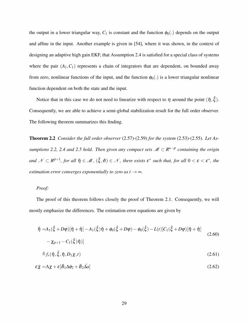
Notice that in this case we do not need to linearize with respect to η around the point (η , ξ ).

Consequently, we are able to achieve a semi-global stabilization result for the full order observer.

The following theorem summarizes this finding.

Theorem 2.2 Consider the full order observer (2.57)-(2.59) for the system (2.53)-(2.55). Let As-

sumptions 2.2, 2.4 and 2.5 hold. Then given any compact sets M ⊂ Rn−ρ containing the origin

and N ⊂ Rρ+1, for all η ∈M , (ξ , σ) ∈ N , there exists ε∗ such that, for all 0 < ε < ε∗, the

estimation error converges exponentially to zero as t→ ∞.

Proof:

The proof of this theorem follows closely the proof of Theorem 2.1. Consequently, we will

mostly emphasize the differences. The estimation error equations are given by

˙η =A1(ξ +Dϕ)[η + η ]−A1(ξ )η +φ0(ξ +Dϕ)−φ0(ξ )−L(t)[C1(ξ +Dϕ)[η + η ]

−χρ+1−C1(ξ )η)]

(2.60)

, fr(η , ξ , η ,D1χ, t) (2.61)

ε χ =Λχ + ε[B1∆φ2 + B2∆a] (2.62)

29

where η ,χ,ϕ,D,D1, B1, B2, ∆a and Λ are defined in Section 2.4, χρ+1 =C1(ξ )η− σ and ∆φ2 =

φ2(η + η , ξ +Dϕ,u)− φ2(η , ξ ,u). Setting ε = 0, we get χ = 0, and the reduced system ˙η =

[A1(ξ )− LC1(ξ )]η . Using the bounds (2.19), (2.20) and (2.29), it can be shown that V1(t, η) =

ηT P−1η satisfies

∂V1

∂ ηfr(η ,0, t)≤−c1 ||η ||2 , ∀ η ∈ Rn−ρ , ∀ t ≥ t0 (2.63)

where c1 is a positive constant independent of ε . Choose a positive constant c such that c >

maxη∈MV1(t, η). This yields M ⊂ Ωt,c = V1(t, η) ≤ c ⊂ Rn−ρ . The rest of the proof follows

identical arguments to the proof of Theorem 2.1.

2.5.1 Observer Design For The Translating Oscillator With a Rotating Ac-

tuator System

Consider the problem of designing a full order observer for a Translating Oscillator with a Rotating

Actuator (TORA) system. The model equations in the normal form are given by [60], [61]

η1 =η2 (2.64)

η2 =k

mr +mc

(mrlr sinξ1

mr +mc−η1

)(2.65)

ξ1 =ξ2 (2.66)

ξ2 =1

δ (ξ1)

(mr +mc)u−mrlr cosξ1

[mrlrξ 2

2 sinξ1− k(

η1−mrlr sinξ1

mr +mc

)](2.67)

y =ξ1 (2.68)

where δ (ξ1) = (I+mrl2r )(mr+mc)−m2

r l2r cos2 ξ1 > 0. mr and I are the mass and moment of inertia

of the rotating proof mass, respectively, lr is the distance from its rotational axis, mc is the mass of

30

the platform, and k is the spring constant. The normal form (2.64)-(2.68) was obtained using the

change of variables

ξ1 = θ , ξ2 = θ , η1 = xc +mrlr sinθ

mr +mcand η2 = xc +

mrlrθ cosθ

mr +mc,

where θ is the angular position of the proof mass (measured counter clock wise) and xc is the

translational position of the platform. We assume that y is the only measured variable. This system

has the special form (2.53)-(2.55) and is not minimum phase. The auxiliary system is given by

(2.64)-(2.65) with the output

σ =kmrlr cosy

δ (y)η1.

Following the technique presented in this section, a full order observer for the system (2.64)-(2.68)

can be taken as

˙ξ1 =ξ2 +(α1/ε)(y− ξ1) (2.69)

˙ξ2 =σ +a(ξ ,u)+(α2/ε

2)(y− ξ1) (2.70)

˙σ =φ2(η , ξ )+(α3/ε3)(y− ξ1) (2.71)

˙η1 =η2 +L1(σ −kmrlr cosy

δ (y)η1) (2.72)

˙η2 =k

mr +mc(mrlr sinymr +mc

− η1)+L2(σ −kmrlr cosy

δ (y)η1), (2.73)

where

a(ξ ,u) =1

δ (y)[(mr +mc)u−

m2r l2

r k sinycosymr +mc

−m2r l2

r ξ22 sinycosy],

and

φ2(η , ξ ) =kmrlrη2 cosy

δ (y)− kmrlrη1ξ2

δ (y)2 [δ (y)siny+2m2r l2

r cos2 ysiny].

31

The observer gain L = [L1 L2]T , is given by (2.17), and P is the solution of (2.18). The matrices A1

and C1 are

A1 =

0 1

−k/(mr +mc) 0

, C1 =

[(kmrlr cosy)/δ (y) 0

].

We will examine the performance of the observer when the system is stabilized by a control u that

is given by [61]

u =−β sat

(ξ2 + k2y− k1(η1− (mrlr siny)/(mr +mc))cosy

µ

)(2.74)

where the positive constants k1, k2, β and µ are design parameters and sat(·) is the saturation

function. After an exhaustive search it was found that the system (2.64)-(2.68) with (2.74), under

state feedback, has a reasonable performance for the following ranges of the initial states: η1(0) =

[−0.1,0.1],η2(0) = [−0.1,0.1],ξ1(0) = [−2π,2π] and ξ2(0) = [−10,10]. We also found that,

for these ranges, ξ1 ∈ [−10,10], ξ2 ∈ [−55,55] and σ ∈ [−140,140]. Consequently, we chose to

saturate ξ1, ξ2 and σ at the values±15,±60 and±145, respectively, to guard against peaking. The

system was simulated using the following system parameters [61]: mc = 1.3608kg, mr = 0.096kg,

lr = 0.0592m, I = 0.0002175kgm2, k = 186.3N/m. The controller parameters are chosen as:

k1 = 1000, k2 = 5, β = 0.2 and µ = 0.1, and the observer parameters are chosen to be: ε = 0.003,

α1 = 3, α2 = 3, α3 = 1, R = 1 and Q =

0.8 0

0 0.8

. The initial values are chosen as: ξ1(0) = 0.5,

ξ2(0) = 1, η1(0) = 0.05, η2(0) = 0.05, ξ1(0) = 0, ξ2(0) = 0, η1(0) = 0, η2(0) = 0 and P(0) =1 0

0 1

.

Figs. 2.3 and 2.4 show the original system states (θ , xc, xc) and their estimates. It is clear that

the observer reconstructed the system states fairly quickly.

32

0 1 2 3 4 5 6 7−40

−20

0

20

40

60

Time (sec)

θ

ˆθ

Figure 2.3: Estimation of the state θ .

0 1 2 3 4 5 6 7−0.2

0

0.2

0 1 2 3 4 5 6 7−1

0

1

Time (sec)

xc

xc

xc

ˆxc

Figure 2.4: Estimation of the internal states xc and xc.

33

2.6 Conclusions

We have proposed a full order observer for a class of nonlinear systems that could be non-minimum

phase. The observer is based on the use of the EHGO to estimate, in a relatively fast time, the

derivatives of the output and a signal that is used as a virtual output to an auxiliary system com-

prised of the internal dynamics. Accordingly, we chose to design an EKF observer for this system.

The reason for this choice is primarily because of the EKF’s simplicity and wide use in practice.

If the system is linear in the internal state we achieve non-local convergence results. In the gen-

eral case, the convergence result is local in the estimation error of the internal states. Finally, we

demonstrated the effectiveness of the proposed observer by using it to estimate the full state vec-

tor for two systems, namely, a synchronous generator connected to an infinite bus and the TORA

system.

34

Chapter 3

Output Feedback Stabilization of Possibly

Non-Minimum Phase Nonlinear Systems

3.1 Introduction

There have been many results in the literature regarding the problem of output feedback stabiliza-

tion of nonlinear systems. In recent years, more attention was directed towards the study of non-

minimum phase nonlinear systems. One of the early papers to study stabilization of non-minimum

phase nonlinear systems is [37]. This paper proves semi-global stabilization for a general class of

non-minimum phase nonlinear systems assuming the existence of a dynamic stabilizing controller

for an auxiliary system. The same problem was considered in [31], where robust semi-global sta-

bilization was achieved under similar assumptions but with an extended high-gain observer-based

output feedback controller.

Papers [39], [40], [38] and [6] solve the problem of output feedback stabilization for nonlinear

systems that can have unstable zero dynamics. Paper [39] allows model uncertainty and is based

on the observer introduced in [32]. Paper [40] assumes the system will be minimum phase with

respect to a new output, defined as a linear combination of the state variables. Paper [38] assumes

the knowledge of an observer and provides different approaches to design the control law. Papers

[39], [40] and [38] achieve global stabilization results under various stabilizability conditions on

35

the internal dynamics. Paper [6] solves the stabilization problem for systems with linear zero

dynamics. It uses the backstepping technique and an observer with linear error dynamics to achieve

semi-global stabilization. Another result reported in [41] deals with a special case of the normal

form where the internal dynamics are modelled as a chain of integrators. It uses an adaptive output

feedback controller, based on Neural Networks and a linear state observer, to achieve ultimate

boundedness of the states in the presence of model uncertainties.

We make use of the Extended High-Gain Observer-Extended Kalman Filter (EHGO-EKF) ap-

proach, proposed in Chapter 2, to solve the problem of output feedback stabilization. In Chapter

2, we showed that we could use the extended high-gain observer to provide the derivatives of the

measured output plus an extra derivative. This extra state is then used to provide a virtual output

that can be used to make the internal dynamics observable. An extended Kalman filter can then

use the virtual output to provide estimates of the remaining states; this is indeed possible thanks to

the difference in time scale provided by the EHGO. The advantage of this observer is that it allows

us to design the feedback control as if all the state variables were available. This is in contrast to

previous high-gain observer results, which were mostly limited to partial state feedback and hence

only to minimum phase systems.

In Chapter 2, we considered systems in the general normal form and proved local convergence

for the EHGO-EKF observer. In the special case when the system is linear in the internal states,

we proved a semi-global convergence result. The work presented in this chapter is related to

this special case.1 We show that when the observer is used in feedback control we can achieve

semi-global stabilization. We allow the use of any globally stabilizing state feedback control.

Furthermore, the class of systems considered includes non-minimum-phase systems. The proposed

1In this chapter, however, we allow the system to depend on the control in a more generalmanner.

36

controller has the ability to recover the state feedback response of an auxiliary system that is based

on the original system. This is beneficial as we can shape the response of the auxiliary system

using the state feedback control as desired, with the knowledge that we will be able to recover it

using the proposed output feedback.

The rest of the chapter is organized as follows. Section 3.2 describes the class of systems and

formulates the problem. In Section 3.3, we describe the output feedback control and state two

theorems that describe the stability and trajectory recovery properties of the closed loop system.

Section 3.4 presents an example of stabilizing a DC-to-DC boost converter system to illustrate the

design procedure with simulation. Finally, Section 3.5 includes some concluding remarks.

3.2 Problem Formulation

We consider a single-input, single-output nonlinear system in the form

η = A1(ξ ,u)η +φ0(ξ ,u) (3.1)

ξ = Aξ +B[C1(ξ ,u)η +a(ξ ,u)] (3.2)

y =Cξ (3.3)

where η ∈ Rn−ρ ,ξ ∈ Rρ , y is the measured output and u is the control input. The ρ ×ρ matrix

A, the ρ × 1 matrix B and the 1×ρ matrix C represent a chain of ρ integrators and the functions

A1(., .),φ0(., .),C1(., .) and a(., .) are known.

In the case that the nonlinear functions A1,φ0 and C1 are independent of the control u, (3.1)-

(3.3) is a special case of the normal form [56], where the system dynamics are linear in the internal

state η . An example of systems of this type is the Translating Oscillator with a Rotating Actuator

37

(TORA) system [60].

Assumption 3.1 The functions A1(ξ ,u), φ0(ξ ,u), a(ξ ,u) and C1(ξ ,u) are sufficiently smooth.

Furthermore, φ0(0,0) = 0 and a(0,0) = 0.

The goal is to stabilize the origin of the system (3.1)-(3.3) using only the measured output y.

3.3 State Feedback

We consider the system (3.1)-(3.3), and assume the existence of globally stabilizing state feedback

control of the form

u = γ(η ,ξ ) (3.4)

Rewrite the full state vector as ϑ = [ηT ξ T ]T , so the closed loop system will be

ϑ = f (ϑ ,γ(η ,ξ )) (3.5)

The control should have the following properties.

Assumption 3.2 1. γ is continuously differentiable with locally Lipschitz derivatives and γ(0,0)=

0.

2. The origin of the closed-loop system (3.5) is globally asymptotically stable.

38

3.4 Output Feedback

In this section, we will design an output feedback controller that is based on the observer

˙ξ = Aξ +B[σ +a(ξ ,u)]+H(ε)(y−Cξ ) (3.6)

˙σ = φ1(η , ξ )+(αρ+1/ερ+1)(y−Cξ ) (3.7)

˙η = A1(ξ ,u)η +φ0(ξ ,u)+L(t)(M1sat(σ

M1)−C1(ξ ,u)η) (3.8)

where φ1(η ,ξ ) is the derivative of C1(ξ ,u)η under the state feedback control u = γ(η ,ξ ), i.e.,

φ1(η ,ξ ) =∂ [C1(ξ ,γ(η ,ξ ))η ]

∂η[A1(ξ ,γ(η ,ξ ))η +φ0(ξ ,γ(η ,ξ ))]

+∂ [C1(ξ ,γ(η ,ξ ))η ]

∂ξ[Aξ +B[C1(ξ ,γ(η ,ξ ))η +a(ξ ,γ(η ,ξ ))]]

The observer gain H(ε) is given by

H(ε) = [α1/ε, ...,αρ/ερ ]T .

The constants α1, ...,αρ+1 are chosen such that the polynomial sρ+1+α1sρ + ...+αρ+1 is Hurwitz

and ε > 0 is a small parameter. The observer gain L(t,ε) is given by

L = PCT1 R−1 (3.9)

and P(t,ε) is the solution of the Riccati equation

P = A1P+PAT1 +Q−PCT

1 R−1C1P, P(t0) = P0 > 0. (3.10)

39

where A1(., .) and C1(., .) are functions of ξ and γ(η , ξ ), R(t) satisfies

0 < r1 ≤ R(t)≤ r2 (3.11)

and Q(t) is a symmetric positive definite matrices that satisfies

0 < q1In−ρ ≤ Q(t)≤ q2In−ρ (3.12)

The observer (3.6)-(3.8) is to be used with the control

u = γ(η , ξ ). (3.13)

Assumption 3.3 The nonlinear functions A1(ξ ,γ(η , ξ )), φ0(ξ ,γ(η , ξ )),

a(ξ ,γ(η , ξ )), C1(ξ ,γ(η , ξ )), γ(η , ξ ) and φ1(η , ξ ) are globally bounded in ξ .

The assumption of global boundedness in ξ , which comes from the extended high-gain ob-

server, is essential to protect against peaking. It is not restrictive, as it can be done by using

saturation outside compact sets to which the trajectories belong to under state feedback [22]. The

saturation functions need to be also continuously differentiable.2 The variable σ is saturated in

(2.59) using the standard sat(.) function. This is to prevent peaking in η . The saturation level M1

is determined such that M1 ≥ max |C1(ξ ,u)η | under state feedback. This procedure is illustrated

in the example presented in Section 3.5.

2Reference [26] shows an example of a continuously differentiable saturating function andalso an approach on how to analyze the system in the case of the standard piecewise-continuoussaturation function.

40

Assumption 3.4 The Riccati equation (3.10) has a positive definite solution that satisfies

0 < p1In−ρ ≤ P−1(t)≤ p2In−ρ , ∀ t ≥ 0 (3.14)

This assumption is essential for the stability of the EHGO-EKF observer as will be shown in the

proof of Theorem 3.1.3

We will study the properties of the closed loop system with the estimation error dynamics. To

that end, let us use the following rescaling of the estimation error:

η = η− η (3.15)

χi = (ξi− ξi)/ερ+1−i, 1≤ i≤ ρ (3.16)

χρ+1 =C1(ξ ,γ(η ,ξ ))η− σ (3.17)

Let ϕ = [χ1,χ2, ...,χρ ]T and D(ε) = diag[ερ ,ερ−1, ...,ε] so that (3.16) becomes

D(ε)ϕ = ξ − ξ . (3.18)

Moreover, let χ = [ϕT χρ+1]T and D1(ε) = diag[D, 1], thus we have,

D1(ε)χ =

ξ − ξ

C1(ξ ,γ(η ,ξ ))η− σ

.3Examples of classes of systems where this assumption is satisfied can be found in [55], [50]

and in the context of designing an adaptive high gain observer in [54].

41

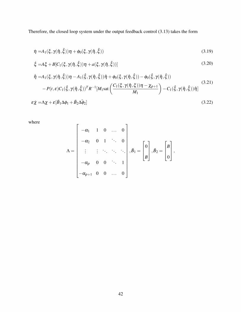
Therefore, the closed loop system under the output feedback control (3.13) takes the form

η =A1(ξ ,γ(η , ξ ))η +φ0(ξ ,γ(η , ξ )) (3.19)

ξ =Aξ +B[C1(ξ ,γ(η , ξ ))η +a(ξ ,γ(η , ξ ))] (3.20)

˙η =A1(ξ ,γ(η , ξ ))η−A1(ξ ,γ(η , ξ ))η +φ0(ξ ,γ(η , ξ ))−φ0(ξ ,γ(η , ξ ))

−P(t,ε)C1(ξ ,γ(η , ξ ))T R−1[M1sat(

C1(ξ ,γ(η ,ξ ))η−χρ+1

M1

)−C1(ξ ,γ(η , ξ ))η ]

(3.21)

ε χ =Λχ + ε[B1∆φ1 + B2 ¯∆φ2] (3.22)

where

Λ =

−α1 1 0 . . . 0

−α2 0 1 . . . 0

...... . . . . . . . . .

−αρ 0 0 . . . 1

−αρ+1 0 0 . . . 0

, B1 =

0

B

, B2 =

B

0

,

42

∆φ1 =φ1(η ,ξ , η , ξ ,ε)−φ1(η , ξ ),

φ1(η ,ξ , η , ξ ,ε) =[∂C1(ξ ,γ(η ,ξ ))η ]

∂ξ[Aξ +B[C1(ξ ,γ(η , ξ ))η +a(ξ ,γ(η , ξ ))]]

+C1(ξ ,γ(η ,ξ ))[A1(ξ ,γ(η , ξ ))η +φ0(ξ ,γ(η , ξ ))]

+[∂C1(ξ ,γ(η ,ξ ))η ]

∂ η[A1(ξ ,γ(η , ξ ))η +φ0(ξ ,γ(η , ξ ))

+P(t)C1(ξ ,γ(η , ξ ))T R−1×

[M1sat(

C1(ξ ,γ(η ,ξ ))η−χρ+1

M1

)−C1(ξ ,γ(η , ξ ))η ]],

∆φ2 =∆φ3/ε,

∆φ3(η ,ξ , η , ξ ) =a(ξ ,γ(η , ξ ))−a(ξ ,γ(η , ξ ))+C1(ξ ,γ(η , ξ ))η−C1(ξ ,γ(η ,ξ ))η .

It can be shown that, for all (η ,ξ , η ,D(ε)ϕ) ∈ Q ⊂ R2n where Q is a compact set, ∆φ2 is locally

Lipschitz and bounded from above by linear in ||χ|| function, uniformly in ε . The matrix Λ is

ρ + 1× ρ + 1 Hurwitz by design. Using (3.15) and (3.18), it can be seen that the closed-loop

system has an equilibrium point at the origin η = η = 0 and ξ = ξ = 0. We also notice that the

sat(.) function has no effect at the origin. Therefore, it is not difficult to show that ∆φ1 = 0 and

∆φ2 = 0 at the origin. Based on the above observations, we see that the system (3.19)-(3.22) is

in the standard singularly perturbed form and has an equilibrium point at the origin. It should

be noted that (3.10) is part of the estimation error dynamics and has the property mentioned in

Assumption 3.4. However, in what follows, we will only show stability of the origin of the system

(3.19)-(3.22).

43

3.4.1 Stability Recovery

Let us define the initial states as (η(0),ξ (0), η(0)) ∈M and (ξ (0), σ(0)) ∈N , where M , con-

taining the origin, and N are any known compact subsets of R2n−ρ and Rρ+1, respectively. Thus,

we have

η(0) = η(0)− η(0), ϕ(0) = D−1(ε)[ξ (0)− ξ (0)]

and

χρ+1(0) =C1(ξ (0),γ(η(0),ξ (0)))η(0)− σ(0).

We are now ready to present the following theorem, which describes the stability properties of the

closed-loop system under output feedback control.

Theorem 3.1 Consider the closed loop system (3.19)-(3.22). Let Assumptions 3.1-3.4 hold. Then

for trajectories (η ,ξ , η)× (ξ , σ), starting in M ×N , we have the following

• There exists ε∗1 , such that for all 0 < ε < ε∗1 , the origin of the closed loop system is asymp-

totically stable and M ×N is a subset of its region of attraction.

• If the origin of the system (3.5) is exponentially stable then, there exists ε∗2 , such that for all

0 < ε < ε∗2 , the origin of the closed loop system is exponentially stable and M ×N is a

subset of its region of attraction.

Proof:

For convenience, rewrite (3.19)-(3.20) as ϑ , fa(ϑ , η ,Dϕ) and (3.21) as ˙η = fb(ϑ , η , t,D1χ).

Assumption 3.2 and the converse Lyapunov theorem, see [[61], Th. 4.17], imply the existence of

a smooth positive definite radially unbounded function V1(ϑ), and a continuous positive definite

function α(ϑ), such that

∂V1

∂ϑfa(ϑ ,0,0)≤−α(ϑ), ∀ϑ ∈ Rn (3.23)

44

Recall that ς = [ηT ξ T ηT ]T and consider the composite Lyapunov function candidate V3(t,ς) =

qV1(ϑ)+ (ηT P−1η)1/2 for the system (3.19)-(3.21), where q is a positive constant to be chosen.

It can also be argued from the positive definiteness of V1, see [[61], Lemma 4.3], and (3.14) that

there exist class K∞ functions β1 and β2 such that V3 satisfies

β1(||ς ||)≤V3(t,ς)≤ β2(||ς ||) (3.24)

Define Ω , V3(t, η) ≤ c. For any c > 0, β2(||ς ||) ≤ c is a compact subset of R2n−ρ . Now

choose c > max(ϑ ,η)∈M

β2(||ς ||) so that M ∈ β2(||ς ||) ∈Ω ∈ R2n−ρ .

Consider, for the system (2.35), the Lyapunov function candidate

W (χ) = χT P0χ, (3.25)

where P0 is the positive definite solution of P0Λ+ΛT P0 =−I. This Lyapunov function satisfies

λmin(P0) ||χ||2 ≤W (χ)≤ λmax(P0) ||χ||2 ,

where λmin(P0) and λmax(P0) are the minimum and maximum eigenvalues of P0, respectively.

Let Σ = W (χ) ≤ βε2 and S = Ω×Σ, where β is a positive constant independent of ε to

be defined later. In what follows, we prove that the set S is positively invariant and then we will

prove that all the trajectories enter this set in finite time. Furthermore, we will prove the stability

of the origin over this set. For this purpose, we notice that for any 0 < ε1 ≤ 1, there are L1 and L2,

45

independent of ε , such that for all (ς ,χ) ∈S and every 0 < ε ≤ ε1 and t ≥ 0, we have

|| fa(ϑ , η ,Dϕ)− fa(ϑ , η ,0)|| ≤ L1 ||χ|| (3.26)

|| fb(ϑ , η , t,D1χ)− fb(ϑ , η , t,0)|| ≤ L2 ||χ|| (3.27)

|| fa(ϑ , η ,Dϕ)− fa(ϑ ,0,Dϕ)|| ≤ L3 ||η || (3.28)

where we used the facts ||D1|| ≤ 1,||ϕ|| ≤ ||χ|| and sat(.) is globally Lipschitz. From Assumption

3.1 and for all ς ∈ Ω (knowing the fact that continuous functions are bounded over compact sets)

and from Assumption 3.3 and for all χ ∈ Rρ+1 (noting that we are saturating σ outside the set Ω),

it can be verified that

||∆φ1(ς ,D1χ)|| ≤ k5 (3.29)

where k5 is positive constant independent of ε . It is worth emphasizing that the function ∆φ1 is

bounded uniformly in ε because the saturation of σ occurs outside a compact set that is indepen-

dent of ε . Using (3.11), (3.12), (3.14), (3.26), (3.28) (3.27), (3.29), continuous differentiability of

V1, Lipschitz properties of fa and fb and noting that P−1

dt =−P−1PP−1, it can be shown that

V3 ≤−qα3(||ϑ ||)+(qL3d− k1

2√

p1) ||η ||+ k2ε (3.30)

W ≤− (h1

ε−h3)W +h2

√W (3.31)

where k1 is positive constant dependent on the bounds (3.11), (3.12) and (3.14), k2 = (qdL1 +

(p2L2)/(2√

p1))√

β/λmin(P0) and d is positive constant such that d > ||∂V1/∂ϑ || over Ω, and h1,

h2 and h3 are positive constants independent of ε . It can be shown that there exists εa > 0 and β

large enough such that, for all 0 < ε ≤ εa and (ς ,χ) ∈Ω×W = βε2, (3.31) is negative definite.

46

For this value of β , it can be shown that, for q < k1/(2L3d√

p1) there exists εb > 0 such that, for

every 0 < ε < εb, and (ς ,χ) ∈ V3 = c×Σ, we have V3 ≤ 0. Choose ε2 = minεa,εb, then the

set S is positively invariant for all 0 < ε ≤ ε2.

Consider the trajectories (ς(t), ξ (t), σ(t)) starting in the set M ×N , it can be verified that

there exists a finite time T0 independent of ε such that ς(t) ∈ Ω for all t ∈ [0,T0]. During this

time, χ will be bounded by an O(1/ερ) value. Moreover, there exists ε3 > 0 and T (ε) > 0 with

T (ε)→ 0 as ε → 0, such that W (χ(T (ε))) ≤ βε2 for every 0 < ε < ε3. Therefore, taking ε∗0 =

minε1,ε2,ε3 ensures that the trajectory (ς ,χ) enters the set S during the time interval [0,T (ε)],

for every 0 < ε < ε∗0 , and does not leave thereafter.

We can now work locally inside the set S to prove asymptotic stability of the origin. To

this end, we first consider the Lyapunov function candidate V4(t, η ,χ) =V1(ϑ)+θ1√

ηT P−1η +√W (χ), where θ1 > 0 to be determined. Using the continuous differentiability of V1, the Lipschitz

properties of fa and fb, ∆φ1 and ∆φ2, it can be shown that, for all (ϑ , η ,χ) ∈S , we have

V4 ≤−α3(||ϑ ||)− [a1θ1−a2] ||η ||− [a3(1ε−a4)−θ1a5] ||χ|| (3.32)

where a1 to a5 are positive constants. Choosing θ1 > a2/a1 and 0 < ε∗1 ≤ ε∗0 such that ε∗1 <

1/((θ1a5)/a3 +a4), then, for all 0 < ε ≤ ε∗1 , V4 is negative definite. This proves the first bullet.

To prove the second bullet, we define a ball B(0,r1), for some radius r1 > 0 inside the set S and

around the origin (ς ,χ) = (0,0). Since the origin of the closed loop system (3.5) is exponentially

stable, there exists a Lyapunov function V5 that satisfies the following inequalities for all ϑ ∈

47

B(0,r1) [[61], Th. 4.14]

b1 ||ϑ ||2 ≤V5(ϑ)≤ b2 ||ϑ ||2 (3.33)

∂V7

∂ϑf (ϑ ,γ(η ,ξ ))≤−b3 ||ϑ ||2 (3.34)∣∣∣∣∣∣∣∣∂V5

∂ϑ

∣∣∣∣∣∣∣∣≤ b4 ||ϑ || (3.35)

for some positive constants b1,b2,b3 and b4. Consider now the composite Lyapunov function

V6(t,ϑ , η) =V5(ϑ)+θ1ηT P−1η +W (χ) with θ1 > 0. Choose r2 < r1, then it can be shown, using

(3.45), (3.34), (3.35), Lipschitz properties of fa and fb that for all (ϑ , η ,χ) ∈ B(0,r2)×||η || ≤

r2×||χ|| ≤ r2, we have

V6 ≤−b3 ||ϑ ||2 + c1 ||ϑ || ||η ||+ c2 ||ϑ || ||χ||−θ1c3 ||η ||2 +θ1c4 ||η || ||χ||

− [1ε− c5] ||χ||2 + c6 ||η || ||χ||

≤−

||ϑ ||

||η ||

||χ||

T b3 −c1/2 −c2/2

−c1/2 θ1c3 −(θ1c4 + c6)/2

−c2/2 −(θ1c4 + c6)/2 [1/ε− c5]

||ϑ ||

||η ||

||χ||

,−

||ϑ ||

||η ||

||χ||

T

Γ

||ϑ ||

||η ||

||χ||

,

where c1 to c6 are positive constants. Choose θ1 to make z , θ1b3c3− c21/4 positive and ε∗2 > 0

small enough such that, for all 0 < ε ≤ ε∗2 , the determinant of Γ is positive. This makes Γ a positive

definite constant matrix, which makes V6 negative definite. This completes the proof.

48

3.4.2 Trajectory Recovery

In this section, we will show that the output feedback system proposed in this chapter has the

ability to recover the performance of an auxiliary system working under state feedback. To that

end, let ς(t,ε) be the solution of the system (3.19)-(3.21), where ς = [ηT ξ T ηT ]T = [ϑ T ηT ]T , and

ςr(t) be the solution of

ϑ = f (ϑ ,γ(η− η ,ξ )) (3.36)

˙η = [A1(ξ ,γ(η− η ,ξ ))− L(t)C1(ξ ,γ(η− η ,ξ ))]η (3.37)

starting from ς(0), where L(t) = P(t)C1(ξ ,γ(η− η ,ξ ))R−1 and P(t) is the solution of the Riccati

equation

˙P = A1P+ PAT1 +Q− PCT

1 R−1C1P, P(t0) = P0 (3.38)

where A1(., .) and C1(., .) are functions of ξ and γ(η ,ξ ), P0 is the initial condition of (3.10) and

R(t) and Q(t) satisfy (3.11) and (3.12), respectively. Notice that this Riccati equation is different

than (3.10), which makes use of both η and ξ .

Assumption 3.5 The Riccati equation (3.38) has a positive definite solution that satisfies

0 < p1In−ρ ≤ P−1(t)≤ p2In−ρ , ∀ t ≥ 0 (3.39)

and a steady state solution Pss.

49

Define

Perror(t) = P(t)− Pss(t) =

P11 P12 ... P1(n−ρ)

......

......

P(n−ρ)1 P(n−ρ)2 ... P(n−ρ)(n−ρ)

(n−ρ)×(n−ρ)

,

and stack the elements of Perror to form the following vector

˜P = [P11...P1(n−ρ)...Pi1...Pi(n−ρ)...P(n−ρ)1...P(n−ρ)(n−ρ)]T ,

where 1 < i < n−ρ.

Assumption 3.6 The origin of the system

˙P = fc(t, ˜P, η ,ξ ) (3.40)

is exponentially stable.

We are now ready to have the following result.

Theorem 3.2 Let Assumptions 3.1-3.6 hold. If the origin of the system (3.5) is exponentially sta-

ble, then, given any µ > 0, there exists ε∗3 > 0 such that, for sufficiently small∣∣∣∣∣∣ ˜P(0)

∣∣∣∣∣∣ and for

trajectories starting in M ×N , where M is sufficiently small, and for every 0 < ε ≤ ε∗3 , we have

||ς(t,ε)− ςr(t)|| ≤ µ, ∀ t ≥ 0. (3.41)

Remark 3.1 If all the conditions hold globally, then Theorem 3.2 is valid for trajectories starting

in any M ×N .

50

Proof :4

Consider the change of variables P∗(t) = P(t)− Pss(t). Then we can observe that the closed

loop system (3.19)-(3.22) with

˙P = fg(t, P,ϑ , η ,Dϕ), (3.42)

where P is a vector that contains the elements of P∗(t), is in the singularly perturbed form, where

(3.19)-(3.21) and (3.42) constitute the slow dynamics and (3.22) constitutes the fast dynamics.

We also observe that the system (3.36), (3.37) and (3.40) is nothing but the reduced system of

(3.19)-(3.22) and (3.42) when ε = 0; this is because ε = 0 yields χ = 0, which gives ϕ = 0. We

know from the proof of Theorem 3.1 that, there exists ε∗0 > 0 such that, for every 0 < ε ≤ ε∗0 , the

trajectories are inside the set S for all t ≥ T (ε), where S is O(ε) in the direction of the variable

χ . We will start by proving the stability of the reduced system (3.36), (3.37) and (3.40), and then

to accomplish the proof we will use the same approach used to prove Theorem 3 in [35].

For convenience, rewrite (3.36) as ϑ , fd(ϑ , η) = fa(ϑ , η ,0), (3.37) as ˙η , fe(ϑ , η , t) =

fb(ϑ , η , t,0), ς(t,ε), [ςT (t,ε) ˙PT (t)]T , ςr(t), [ςTr (t) ˜PT (t)]T , F(t, ς(t,ε),D1(ε)χ),

fa

fb

fg

and

ς(0) = [ς(0)T PT (0)].

For (3.37), we define the Lyapunov function candidate

V2(t, η) = ηT P−1

η . (3.43)

4we use in this proof the same definitions used in the proof of Theorem 3.1, unless otherwisestated.

51

It can be seen using (3.39) that V2 satisfies

p1 ||η ||2 ≤V2(t, η)≤ p2 ||η ||2 (3.44)

Using the bounds (3.11), (3.12), (3.39), and dP−1

dt =−P−1 ˙PP−1, we obtain

∂V2

∂ t+

∂V2

∂ ηfe(ϑ , η , t) = ˙ηT P−1

η + ηT dP−1

dtη + η

T P−1 ˙η

≤−k1 ||η ||2 , ∀ η ∈ Rn−ρ , ∀ t ≥ 0,

(3.45)

where k1 is a positive constant.

We define a ball B(0,r3), for some radius r3 > 0 around the origin (ϑ , η , ˜P) = (0,0,0). Using

Assumption 3.6 and the converse Lyapunov theorem [[61], Th. 4.14], we know that there exists a

Lyapunov function V7 that satisfies the following inequalities for all ˜P ∈ B(0,r3)

e1

∣∣∣∣∣∣ ˜P∣∣∣∣∣∣2 ≤V7(t, ˜P)≤ e2

∣∣∣∣P∣∣∣∣2 (3.46)

∂V7

∂ t+

∂V7

∂ ˜Pfc(t, ˜P, η ,ξ )≤−e3

∣∣∣∣∣∣ ˜P∣∣∣∣∣∣2 (3.47)∣∣∣∣∣∣∣∣∂V7

∂ ˜P

∣∣∣∣∣∣∣∣≤ e4

∣∣∣∣∣∣ ˜P∣∣∣∣∣∣ (3.48)

for some positive constants e1,e2,e3 and e4. Consider now the composite Lyapunov function

V8(t,ϑ , η , ˜P) = θV2(t, η) +V5(ϑ) +V7(t, ˜P), where V2 is given by (3.43), θ is a positive con-

stant to be chosen and V5 satisfies inequalities (3.33)-(3.35) over the ball B(0,r4) for some ra-

dius r4 > 0 around the origin (ϑ , η , ˜P) = (0,0,0). Notice that fd(ϑ ,0) = f (ϑ ,γ(η ,ξ )). Choose

r5 < minr3,r4, then it can be shown, using (3.45), (4.64) and (3.47) that, for all (ϑ , η , ˜P)

52

∈ B(0,r5)×||η || ≤ r5×B(0,r5),

V8 =∂V5

∂ϑfd(ϑ ,0)+

∂V5

∂ϑ[ fd(ϑ , η)− fd(ϑ ,0)]+θV2 +V7

≤−b3 ||ϑ ||2 +b4L ||ϑ || ||η ||−θk1 ||η ||2− e3

∣∣∣∣∣∣ ˜P∣∣∣∣∣∣2

,−

||ϑ ||||η ||

T b3 −(b4L)/2

−(b4L)/2 θk1

||ϑ ||||η ||

− e3

∣∣∣∣∣∣ ˜P∣∣∣∣∣∣2

where L is the Lipschitz constant of fd over ||η || ≤ r5. Choosing θ > (b24L2)/(4k1b3) makes V8

negative definite. This implies that the origin of the system (3.36),(3.37) and (3.40) is exponentially

stable.

We now divide the interval [0,∞] into three intervals [0,T (ε)], [T (ε),T2] and [T2,∞], where T2

is to be determined, and show (3.41) for each interval.

1- The interval [0,T (ε)].

From Assumptions 3.4 and 3.5, we know that P(t) and P(t) are bounded for all t ≥ 0, therefore,

we can deduce that there exists compact sets Z1 and Z2 such that P ∈ Z1 and ˜P ∈ Z2 for all t ≥ 0. .

Since the vector field F is continuous, we can write

ς(t,ε)− ς(0) =∫ t

0F(t, ς(τ,ε),D1(ε)χ).dτ

Using similar arguments to the ones leading to the inequality (3.29), we can argue that ||F(., ., .)|| ≤

k9, where k9 is some positive constant independent of ε . Consequently, since ς(0) is in the interior

of a compact set, we have

||ς(t,ε)− ς(0)|| ≤ k9t, ∀ς(t,ε) ∈Ω×Z1

53

In the same way, we can show, during the same interval, that

||ςr(t)− ς(0)|| ≤ k9t.

Hence,

||ς(t,ε)− ςr(t)|| ≤ 2k9T (ε), ∀ t ∈ [0,T (ε)]. (3.49)

Since T (ε)→ 0 as ε → 0, there exists 0 < ε4 ≤ ε∗1 such that, for every 0 < ε ≤ ε4, we have

||ς(t,ε)− ςr(t)|| ≤ µ, ∀ t ∈ [0,T (ε)]. (3.50)

2- The interval [T (ε),T2].

During this interval ς(t,ε) satisfies ˙ς = F(t, ς ,D1χ), with initial condition ς(T (ε),ε) and D1χ is

O(ε), and ςr(t) satisfies ˙ς = F(t, ς ,0), with initial condition ςr(T (ε)). From (3.49), we know that

||ς(t,ε)− ςr(t)|| ≤ 2k9T (ε), δ (ε), where δ → 0 as ε→ 0. Therefore, by [Theorem 3.5,[61]], we

conclude that there exists 0 < ε5 ≤ ε∗1 such that for every 0 < ε ≤ ε5, we have

||ς(t,ε)− ςr(t)|| ≤ µ, ∀ t ∈ [T (ε),T2]. (3.51)

3- The interval [T2,∞).

We can show that for any µ > 0, there exists ε∗4 > 0 and T2 ≥ T (ε)> 0, both dependent on µ , such

that, for every 0 < ε ≤ ε∗4 , we have

||ς(t,ε)|| ≤ µ/2, ∀t ≥ T2. (3.52)

54

From the exponential stability of the reduced system, we know that there exits a finite time T2,

independent of ε , such that

||ςr(t)|| ≤ µ/2, ∀t ≥ T2. (3.53)

Take T2 = maxT2, T2. Then, using the triangular inequality, and from (3.52) and (3.53), we

conclude that for every 0 < ε ≤ ε∗4 , we have

||ς(t,ε)− ςr(t)|| ≤ µ, ∀ t ≥ T2. (3.54)

Take ε∗3 = minε4,ε5,ε∗4, then using (3.50),(3.51) and (3.54) we conclude (3.41).

Theorem 3.2 shows that the output feedback control, due to the use of the extended high-gain

observer (3.6)-(3.7), can asymptotically recover the trajectories of the system (3.36)-(3.37). This

is beneficial as, first, it allows us to assume that the states ξ ,η and η are available in the state

feedback design stage, and thus, simplifies the design procedure. In addition, this result can allow

for tuning the control u to satisfy certain performance requirements in the state feedback design

stage. This can be done by simulating equations (3.36)-(3.37) and checking if the trajectories

satisfy the design specifications. Second, it shows that the control design has to take into consid-

eration the estimation error η , which is considered as an input to the closed-loop state feedback

system. Therefore, by using equation (3.37), one can deduce the properties of this input under

output feedback, and hence, can design a state feedback control accordingly.

55

3.5 Output Feedback Control of a DC-to-DC Boost Converter

System

Consider the problem of output feedback stabilization of a DC-to-DC boost converter. The aver-

aged model of the system is described by [62], [63]

˙η =−1L

uξ +EL

˙ξ =−G

Cξ +

1C

uη

y = ξ

(3.55)

where η , ξ represent the inductor current and the capacitor voltage, respectively, and u is a con-

tinuous signal representing the slew rate of a PWM circuit controlling the switch position in the

converter. The inductor, capacitor, load conductance and voltage source are represented by the

positive constants L,C,G and E, respectively.

The objective is to regulate the output voltage ξ to a desired value V∗. This problem can also

be cast as stabilizing the equilibrium point (η∗, ξ∗) = (GV 2∗ /E,V∗) and the corresponding control

u∗ = E/V∗.

We first use the change of variables η = η − η∗, ξ = ξ − ξ∗ and u = u− u∗ to transfer the

equilibrium point to the origin. Accordingly, the system takes the form

η =−ξ

L[u+

EV∗

]− uV∗L

ξ =−Gξ

C+

η

C[u+

EV∗

]+GV 2∗ u

EC

y = ξ

(3.56)

The system (3.56) is non-minimum phase, because the zero dynamics of the linearized system

56

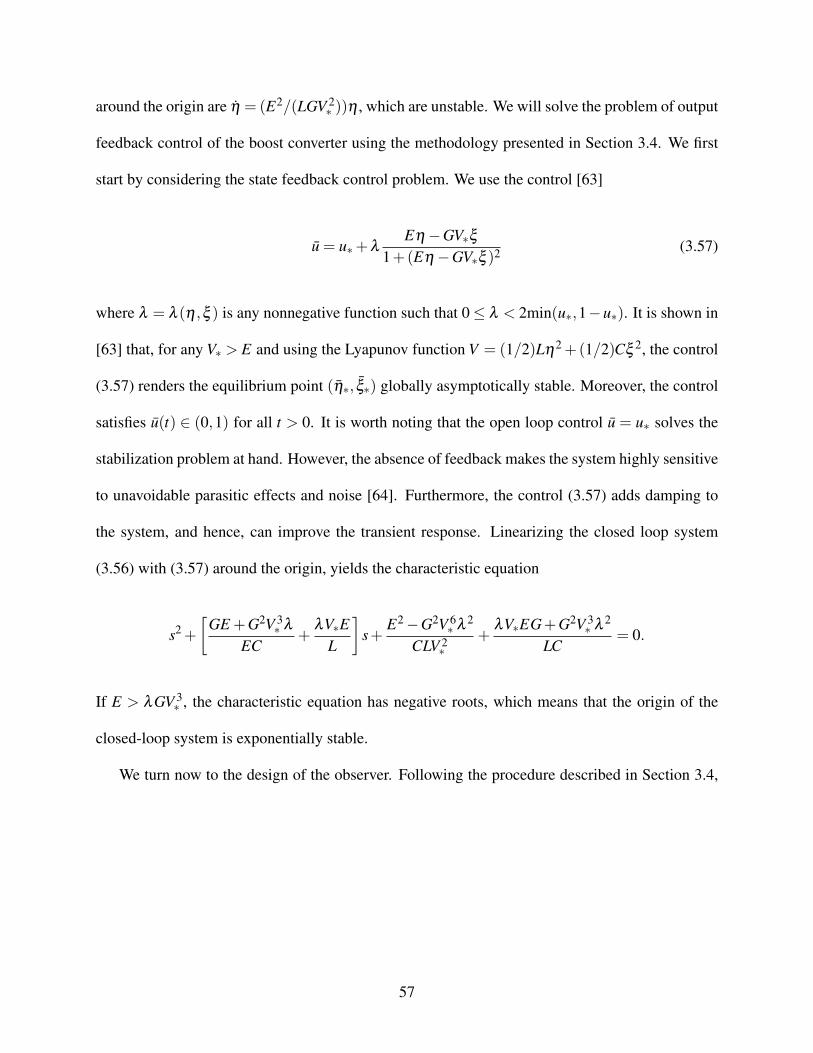
around the origin are η = (E2/(LGV 2∗ ))η , which are unstable. We will solve the problem of output

feedback control of the boost converter using the methodology presented in Section 3.4. We first

start by considering the state feedback control problem. We use the control [63]

u = u∗+λEη−GV∗ξ

1+(Eη−GV∗ξ )2 (3.57)

where λ = λ (η ,ξ ) is any nonnegative function such that 0≤ λ < 2min(u∗,1−u∗). It is shown in

[63] that, for any V∗ > E and using the Lyapunov function V = (1/2)Lη2 +(1/2)Cξ 2, the control

(3.57) renders the equilibrium point (η∗, ξ∗) globally asymptotically stable. Moreover, the control

satisfies u(t) ∈ (0,1) for all t > 0. It is worth noting that the open loop control u = u∗ solves the

stabilization problem at hand. However, the absence of feedback makes the system highly sensitive

to unavoidable parasitic effects and noise [64]. Furthermore, the control (3.57) adds damping to

the system, and hence, can improve the transient response. Linearizing the closed loop system

(3.56) with (3.57) around the origin, yields the characteristic equation

s2 +

[GE +G2V 3

∗ λ

EC+

λV∗EL

]s+

E2−G2V 6∗ λ 2

CLV 2∗

+λV∗EG+G2V 3

∗ λ 2

LC= 0.

If E > λGV 3∗ , the characteristic equation has negative roots, which means that the origin of the

closed-loop system is exponentially stable.

We turn now to the design of the observer. Following the procedure described in Section 3.4,

57

0 0.01 0.02 0.03 0.04 0.0515

16

17

18

Time (sec)

Out

put

Figure 3.1: Output response.

an observer for the system (3.56) is given by

˙ξ =−Gξ

C+ σ +

GV 2∗ u

EC+

α1

ε(y− ξ ) (3.58)

˙σ = φ1(η , ξ )+α2

ε2 (y− ξ ) (3.59)

˙η =− ξ

L(u+

EV∗

)− uV∗L

+1R

PC1(σ −C1η) (3.60)

where, assuming, for convenience, that λ is constant,

φ1(η , ξ ) =(λEη

C(1+(Eη−GV∗ξ )2)+

uV∗+ECV∗

− 2u2ηEλC

)(−ξ

L(u+

EV∗

)− uV∗L

)

+(−λGV∗η

C(1+(Eη−GV∗ξ )2)+

2u2GV∗ηCλ

)(−Gξ

C+

η

C(u+

EV∗

)+GV 2∗ u

EC),

P is the solution of (3.10), A1 = 0 and C1 =1C(u+

EV∗).

It should be mentioned that in this example, where η is scalar, it would be sufficient to use the

extended high-gain observer (3.58)-(3.59) to provide the signal σ , which in turn provides η = σ

C1.

However, we designed the full observer as in Section 3.4 for the purpose of demonstrating the

results of this chapter.

58

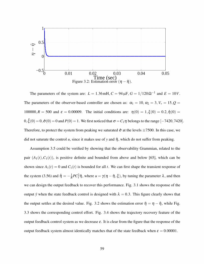
0 0.01 0.02 0.03 0.04 0.05−0.5

0

0.5

1

Time (sec)

η−η

Figure 3.2: Estimation error (η− η).

The parameters of the system are: L = 1.36mH,C = 94µF, G = 1/120Ω−1 and E = 10V .

The parameters of the observer-based controller are chosen as: α1 = 10, α2 = 3,V∗ = 15,Q =

100000,R = 500 and ε = 0.00009. The initial conditions are: η(0) = 1,ξ (0) = 0.2, η(0) =

0, ξ (0)= 0, σ(0)= 0 and P(0)= 1. We first noticed that σ =C1η belongs to the range [−7420,7420].

Therefore, to protect the system from peaking we saturated σ at the levels ±7500. In this case, we

did not saturate the control u, since it makes use of y and η , which do not suffer from peaking.

Assumption 3.5 could be verified by showing that the observability Grammian, related to the

pair (A1(t),C1(t)), is positive definite and bounded from above and below [65], which can be

shown since A1(t) = 0 and C1(t) is bounded for all t. We can first shape the transient response of

the system (3.56) and ˙η =− 1RPC2

1η , where u = γ(η− η ,ξ ), by tuning the parameter λ , and then

we can design the output feedback to recover this performance. Fig. 3.1 shows the response of the

output y when the state feedback control is designed with λ = 0.3. This figure clearly shows that

the output settles at the desired value. Fig. 3.2 shows the estimation error η = η − η , while Fig.

3.3 shows the corresponding control effort. Fig. 3.4 shows the trajectory recovery feature of the

output feedback control system as we decrease ε . It is clear from the figure that the response of the

output feedback system almost identically matches that of the state feedback when ε = 0.00001.

59

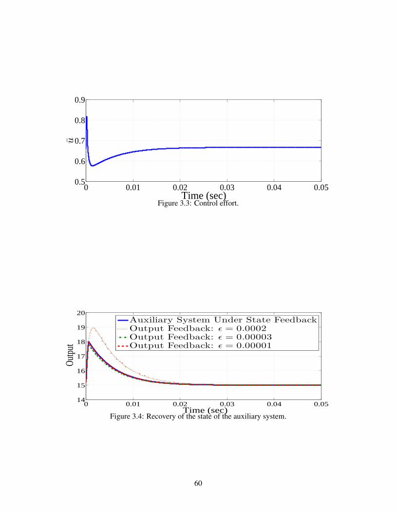
0 0.01 0.02 0.03 0.04 0.050.5

0.6

0.7

0.8

0.9

Time (sec)

u

Figure 3.3: Control effort.

0 0.01 0.02 0.03 0.04 0.0514

15

16

17

18

19

20

Time (sec)

Out

put

Auxiliary System Under State FeedbackOutput Feedback: ǫ = 0.0002Output Feedback: ǫ = 0.00003Output Feedback: ǫ = 0.00001

Figure 3.4: Recovery of the state of the auxiliary system.

60

3.6 Conclusions

We presented an output feedback control strategy that is based on the nonlinear observer proposed

in Chapter 2. The strategy allows for the use of any globally asymptotically stabilizing state feed-

back controller. We proved semi-global stabilization of the origin of the closed-loop system of

a class of nonlinear systems that could be non-minimum phase. We also proved recovery of the

exponential stability of the origin of the closed-loop system under the same conditions. We fi-

nally demonstrated the effectiveness of the proposed control system in stabilizing the DC-to-DC

boost converter system. We also showed that we can shape the transient performance using state

feedback and then we can recover it using output feedback.

61

Chapter 4

Control of Nonlinear Systems Using

Full-Order High Gain Observers: A

Separation Principle Approach

4.1 Introduction

In the previous chapter, we proposed an output feedback control strategy that solves the problem of

semi-global stabilization for a certain class of non-minimum phase nonlinear systems. The struc-

ture of this class is based on the normal form, where the system being linear in the internal state.

The output feedback control is based on an Extended High Gain Observer (EHGO) augmented

with an Extended Kalman Filter (EKF). The idea of this observer was first introduced in Chapter

2; it is based on using EHGO to provide estimates of the output and its derivatives plus a signal

that is used as a virtual output for an auxiliary system comprised of the internal dynamics. The

EKF, called the internal observer, was then used to estimate the states of this auxiliary system.

This approach does not work in the case when the internal dynamics are nonlinear. Therefore, in

this chapter, we propose an output feedback controller that is based on a different observer that is

capable of dealing with nonlinear internal dynamics.

The proposed observer design in this chapter shares the same principle introduced in Chapter

62

2. The new technique used here, nonetheless, is in the design of the internal observer, where now

we propose to use a high-gain observer to estimate the internal states. The challenge in this case,

however, is to ensure that the observer for the output and its derivatives is faster than the internal

observer. This can be realized when we consider the fact that both observers form a high gain

observer that is going to be fast relative to the system dynamics. It turns out that by the use of this

observer, we can achieve a number of properties for the considered class of nonlinear systems. In

particular, it is possible to use any globally stabilizing full state feedback control that is designed

independently of the observer. The output feedback control system can be designed to be robust to

unmatched uncertainties and can totally recover the performance of the state feedback. This would

lead to the assertion of the separation principle along the same lines as in [66].

In Chapter 3, we proposed a feedback control strategy, which is based on the observer pro-

posed on Chapter 2, that solves the problem of semi-global stabilization for a certain class of

non-minimum phase nonlinear systems. The structure of this class is based on the normal form,

where the system is linear in the internal state. However, the approach of Chapter 3, in particular

the observer, can not be adapted for the class of systems considered in this chapter, since this class

of systems is nonlinear in the internal state.

The outline of this chapter is as follows. We start in Section 5.2 with a motivating example of

the design of an output feedback control of flexible joint manipulators using only motor position

feedback. Section 5.3 formulates the problem in a more general setting. Section 5.4 describes the

state feedback stage while Section 5.5 describes the observer design. In Section 5.6, we describe

the structure of the output feedback control scheme and present a theorem that describes the sta-

bility and trajectory recovery properties of the closed loop system. Finally, Section 5.7 includes

concluding remarks.

63

4.2 Motivating Example: Tracking Control of Flexible Joint

Manipulators Using Only Motor Position Feedback

We consider an n-link robot that is described by [67]

D(q1)q1 +C0(q1, q1)q1 +g(q1) = K(q2−q1),

Jq2 +K(q2−q1) = u(4.1)

where q1 ∈ Rn and q2 ∈ Rn represent the link angles and the motor angles respectively, D(q1) is the

n×n positive definite inertia matrix, J is a diagonal positive definite matrix of the actuator inertias,

C0(q1, q1)q1 represents the Coriolis and centrifugal forces, g(q1) represents the gravitational terms,

K is a diagonal positive definite matrix of the joint stiffness coefficients and u ∈ Rn are the applied

torques. Hereafter, we call the q1 dynamics as the link dynamics and q2 dynamics as the motor

dynamics.

It is assumed that the angular part of the kinetic energy of each rotor is due to its own rotation

and that the rotor/gear inertia is symmetric about the rotor axis of rotation. This model shares a

lot of similarities with the rigid robot model, and in fact, reduces to one as K tends to infinity.

The difference lies in the addition of elasticity, which typically is modeled by a linear torsional

spring. For many manipulators, joint flexibility is significant. It is caused by effects such as

shaft windup, bearing deformation, compressibility of the hydraulic fluid in hydraulic robots and

torsional flexibility in the gears [68]. The challenges that are associated with these systems are due

to a number of factors. These systems, first of all, are underactuated since the number of degrees

of freedom is twice the number of control inputs. In addition, there is no matching between the

system nonlinearities and the control input.

64

Motion control of robots with flexible joints has been extensively studied since the 1980s.

Several surveys of the literature are available; see e.g. [69], [70]. Most of the results on output

feedback control of flexible joint manipulators assume at least availability of measurement of either

the link angle, see e.g. [71], [72], or both the link and rotor angles see, e.g. [73], [74]. Another

recent example is the work in [75], which is based on the use of the discrete-time Extended Kalman

Filter (EKF) and assumes availability of the measurements of both motor angle and velocity. In

this chapter, on the other hand, we assume that the only measured variable is the motor angular

position q2. This choice is attractive when it is easier and/or cheaper to measure the motor angular

position. However, this choice might make the system non-minimum phase, as for example in the

case of the single-link manipulator shown in Section 4.2.4 of this chapter, and therefore, makes

the design of the output feedback control scheme more challenging. In general, the motor position

choice as the only measured output was considered in the set-point regulation problem [76], [77],

[78], but, to the best of our knowledge, not in the tracking problem.

We consider the problem of designing an observer-based tracking controller for (4.1). The

objective is to track the link angle q1 using only the measurement of the motor angle q2. We solve

this problem by using ideas from high gain observer theory.

65

4.2.1 Problem Formulation

Using the change of variables η1 = q1, η2 = q1, ξ1 = q2 and ξ2 = q2, the system (4.1) takes the

form

η1 = η2, (4.2)

η2 = φ(η ,ξ ) (4.3)

ξ1 = ξ2, (4.4)

ξ2 = J−1[K(η1−ξ1)+u] (4.5)

y = ξ1 (4.6)

where the system states η ∈ R2n and ξ ∈ R2n are

η = [η11 ,η

12 , ...,η

n1 ,η

n2 ]

T , ξ = [ξ 11 ,ξ

12 , ...,ξ

n1 ,ξ

n2 ]

T ,

and φ(η ,ξ ) = D−1(η1)[K(ξ1−η1)−C(η1,η2)η2− g(η1)]. Equations (4.2)-(4.6) can be written

in the compact form

η = Aη +Bφ(η ,ξ ) (4.7)

ξ = Aξ +B[J−1[K(η1−ξ1)+u]] (4.8)

y =Cξ (4.9)

66

where

A = blockdiag[

A1, ...,An

],Ai =

0 1

0 0

,

B = blockdiag[

B1, ...,Bn

],Bi =

0

1

,C = blockdiag

[C1, ...,Cn

],Ci =

[1 0

],

and i = 1, ...,n

We assume that the function φ(η ,ξ ) is locally Lipschitz in its arguments.

The objective is to design an observer-based output feedback control such that for all suffi-

ciently smooth η1d with bounded derivatives and arbitrary initial conditions (in a known compact

set) we have

limt→∞

(η1−η1d) = 0. (4.10)

4.2.2 Full-State Feedback Control

We first start by considering state feedback control to achieve the goal of tracking with the antici-

pation that we will be able to recover the performance of this control by a high gain observer. To

this end, consider a full state feedback control for the system (4.2)-(4.6) that takes the form

u = γ(η ,ξ ,d(t)). (4.11)

where d(t) ∈ D and D is a compact subset of Rd that includes the reference signal and its deriva-

tives. To solve the problem at hand, we follow the framework used in [79], which considers the

67

change of variables

η1 = η1−η1d (4.12)

η2 = ˙η1 +λ1η1 (4.13)

ξ1 = ξ1−ξ1d (4.14)

ξ2 =˙ξ1 +λ2ξ1 (4.15)

where ξ1d needs to be designed and λ1 > 0,λ2 > 0 are diagonal design matrices.

For convenience, let ϑ =

η

ξ

. Accordingly, the closed-loop state feedback system can be

written as

ϑ = f (ϑ ,γ(η ,ξ ,d(t)),d(t)). (4.16)

We now require the state feedback control design procedure to satisfy:

1. γ is locally Lipschitz in η and ξ uniformly in d.

2. The closed loop system (4.44) is uniformly globally asymptotically stable with respect to the

equilibrium point (η = 0, ξ = 0).

3. The function f (ϑ ,γ(η ,ξ ,d(t)),d(t)) is locally Lipschitz in ϑ , η and ξ uniformly in d.

Moreover, f (ϑ ,γ(η ,ξ ,d(t)),d(t)) is zero at (η = 0, ξ = 0) uniformly in d.

The feedback control may also be required to satisfy extra requirements such as achieving

particular transient response and/or provide robustness to uncertainties.

68

4.2.3 Output Feedback Control

Consider the system (4.2)-(4.6). We propose to use an extended high-gain observer to estimate the

first two derivatives of the output. This would allow us to assume the availability of ξ2 so that we

can use it in estimating the η states. Furthermore, the second derivative of the output represents the

right hand side of (4.5). As a result, as was shown in Chapter 2, it is possible to use this information

to estimate the unknown state η1. We now consider the auxiliary system (4.2)-(4.3) with the signal

σ = J−1Kη1 used as an output. This auxiliary system is in the standard normal form and has a full

relative degree, viewing ξ as an input. Therefore, we can design a high-gain observer to estimate

the η state vector. The crucial point is to design the extended high-gain observer for the output

derivatives so that it is faster than the high-gain observer for the auxiliary system. Based on this

concept, we propose the following full order observer

˙η = Aη +Bφ(η , ξ )+H1(K−1Jσ − η1) (4.17)

˙ξ = Aξ +B[σ − J−1(Kξ1−u)]+H2(y− ξ1) (4.18)

˙σ = J−1Kη2 +H3(y− ξ1) (4.19)

where

H1 = blockdiag[H11, ...,H1n],H1i =

α i1/ε

α i2/ε2

,

H2 = blockdiag[H21, ...,H2n],H2i =

β i1/ε2

β i2/ε4

,H3 = diag[β i

3/ε6]n×n,

69

i = 1, ...,n, (α i1,α

i2) and (β i

1,βi2,β

i3) are chosen such that the polynomials s2 +α i

1s+α i2 and s3 +

β i1s2 +β i

2s+β i3 are Hurwitz, and ε > 0 is a small parameter.

We now replace the states in the state feedback control with their estimates, so that

u = γ(η , ξ ,d(t)) (4.20)

and use the full order observer (4.17)-(4.19) to provide these estimates.

Remark 4.1 To protect against peaking, the auxiliary output σ , and the nonlinear functions φ(η , ξ )

and γ(η , ξ ,d(t)) should be saturated outside their domain under the state feedback control.

It should be noted, however, that there would be no need to saturate φ(η , ξ ) and γ(η , ξ ,d(t)) if

they are originally bounded in η and ξ .

In Section 4.3, we will prove, in a more general setting, that the output feedback control system

recovers the stability properties of the state feedback system. Furthermore, we will show also that

it is possible to recover the system trajectories under state feedback. In the next subsection, we will

demonstrate by simulations these properties along with the behaviour of the system in the presence

of external disturbances and uncertain parameters.

4.2.4 Simulation Example: Single-Link Flexible Joint Manipulators

Consider a single link manipulator with a flexible joint system, where an actuator is connected to

a load through a torsional spring. The equations of motion are given by [67]

70

Jl θl +Mgl sinθl + k(θl−θr) = 0 (4.21)

Jrθr− k(θl−θr) = u (4.22)

where θl,θr,Jl,Jr are the angular positions and the inertias of the link and rotor, respectively, M is

the load mass, l is a distance, g is the gravity, k is the joint stiffness and u is a torque input.

The change of variables η1 = θl, η2 = θl, ξ1 = θr, ξ2 = θr, transforms the model (4.21)−

(4.22) into the normal form

η1 = η2 (4.23)

η2 =−MglJl

sinη1−kJl(η1−ξ1) (4.24)

ξ1 = ξ2 (4.25)

ξ2 =kJr(η1−ξ1)+

1Jr

u (4.26)

y = ξ1 (4.27)

The system (4.23)− (4.27) has a relative degree ρ = 2. The zero dynamics are

η1 = η2 (4.28)

η2 =−MglJl

sinη1−kJl

η1. (4.29)

Using the Lyapunov function candidate

V =∫

η1

0

MglJl

sinz.dz+12

kJl

η21 +

12

η22 ,

71

it can be shown that V = 0, i.e., the system is stable but not asymptotically stable. Thus, the system

is not minimum phase. The objective is to design an output feedback control so that η1 tracks a

desired signal with arbitrarily large region of attraction.

For state feedback control, we use the passivity-based control scheme proposed in [79]. The

control law is given by [79]

u = Jrξ1r + k(ξ1d−η1d)−B2ξ2, (4.30)

with

ξ1d = η1d +1k

uR

uR = Jlη1r +Mgl sin(η1)−B1η2

η1r = η1d−λ1 ˙η1

ξ1r = ξ1d−λ2˙ξ1

where we used the definitions (4.12)-(4.15) and B1,B2 > 0 are design parameters. It is worth

mentioning that the design of the control (4.30) is based on energy shaping technique, where ξ1d

is designed such that the closed loop energy function matches a desired function. Moreover, it can

be shown that the equilibrium point of the closed loop system is globally exponentially stable [79].

We also notice that the control is independent of k. This can be seen by substituting ξ1d back into

(4.30).

72

Following the procedure proposed in Section 4.4, a full order observer can be designed as

˙η1 = η2 +α1

ε(Jr

kσ − η1) (4.31)

˙η2 =−MglJl

sin η1−kJl(η1− ξ1)+

α2

ε2 (Jr

kσ − η1) (4.32)

˙ξ1 = ξ2 +

β1

ε2 (y− ξ1) (4.33)

˙ξ2 = σ +

kJr

ξ1 +1Jr

u+β2

ε4 (y− ξ1) (4.34)

˙σ =kJr

η2 +β3

ε6 (y− ξ1) (4.35)

The system parameters are given as [67]: Jl = 1kg−m2,Jr = 1kg−m2,k = 100N−m/rad,

Mgl = 9.8N−m. The observer and controller constants are chosen to be: ε = 0.06,α1 = 3,α2 =

1,β1 = 5,β2 = 3,β3 = 1,B1 = 7,B2 = 5,λ1 = λ2 = 30. η1d = sin(ωt) with ω = π

3 . The initial values

of the states are chosen as: η1(0) = 0.1,η2(0) = 0.05,ξ1 = 0.1,ξ2 = 0.05, η1(0) = 0, η2(0) =

0, ξ1(0) = 0, ξ2(0) = 0, σ(0) = 0.

4.2.4.1 Case 1: without parameter uncertainties

Fig. 4.1 shows the tracking performance of the link angle η1 to a sinusoidal reference signal

under output feedback control and Fig. 4.2 shows the control effort. It is clear that the con-

trol system achieved good tracking performance. Fig. 4.3 shows the trajectory recovery perfor-

mance of the observer-based output feedback control system. More specifically, it shows the error

(η1)(out put f eedback)− (η1)(state f eedback), where η1 is the tracking error, for different values

of ε . As it can be seen from the figure, the smaller the value of ε , the closer the performance of

the output feedback control gets to the state feedback control. It should be noted that the control u,

η1, η2 and σ were saturated to prevent peaking. The saturation was done for the states that do not

73

0 1 2 3 4 5 6−1.5

−1

−0.5

0

0.5

1

1.5

Time (sec)

Reference SignalLink Angle

Figure 4.1: Tracking of the link angle to a reference signal.

0 1 2 3 4 5 6−200

−150

−100

−50

0

50

100

150

200

Time (sec)

u

Figure 4.2: Control Effort.

74

0 0.5 1 1.5−0.2

−0.15

−0.1

−0.05

0

0.05

Time (sec)

Err

or

ǫ = 0.06ǫ = 0.01ǫ = 0.0001

Figure 4.3: Recovery of the state feedback performance.

constitute the linear part of the observer error dynamics. Furthermore, the saturation was done after

we observed that under state feedback, the control effort needed is in the range [−152,152], η1 is

in the range [−1,1], η2 is in the range [−1.5,1.5] and σ is in the range [−100,100]. Consequently,

we used the saturation levels ±155, ±10, ±10, and ±110 for u η1, η2, and σ , respectively. It is

clear from Fig. 4.2 that the control passed the saturation period in a relatively quick time. We also

tested the performance of the proposed output feedback control system in the presence of measure-

ment noise. Fig. 4.4 shows the tracking error in this case. The noise signal is generated using the

Simulink block “Uniform random Number” with a magnitude limit in the range [−0.0016,0.0016]

and a sampling time of 0.0008 seconds. It is observed from the figure that despite the presence of

noise, the tracking error can reach to a steady state level below 0.05. However, it is noticed, as it is

well known for high gain observers, that there is a trade-off needed between how small can ε get

(or how high can the observer gain get) and sensitivity to noise.

75

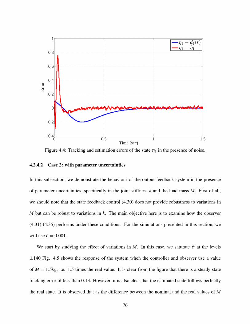
0 0.5 1 1.5−0.4

−0.2

0

0.2

0.4

0.6

0.8

1

Time (sec)

Err

or

η1 − d1(t)η1 − η1

Figure 4.4: Tracking and estimation errors of the state η1 in the presence of noise.

4.2.4.2 Case 2: with parameter uncertainties

In this subsection, we demonstrate the behaviour of the output feedback system in the presence

of parameter uncertainties, specifically in the joint stiffness k and the load mass M. First of all,

we should note that the state feedback control (4.30) does not provide robustness to variations in

M but can be robust to variations in k. The main objective here is to examine how the observer

(4.31)-(4.35) performs under these conditions. For the simulations presented in this section, we

will use ε = 0.001.

We start by studying the effect of variations in M. In this case, we saturate σ at the levels

±140 Fig. 4.5 shows the response of the system when the controller and observer use a value

of M = 1.5kg, i.e. 1.5 times the real value. It is clear from the figure that there is a steady state

tracking error of less than 0.13. However, it is also clear that the estimated state follows perfectly

the real state. It is observed that as the difference between the nominal and the real values of M

76

0 1 2 3 4 5 6−0.2

−0.15

−0.1

−0.05

0

0.05

0.1

0.15

Time (sec)

Tracking ErrorEstimation Error

Figure 4.5: Tracking error and estimation error in the case of uncertain load mass M.

gets bigger the tracking error worsens, but the estimation error remains very close to zero. This

robustness performance by the observer is expected and can be explained by noticing that M is only

present in (4.24), thus, allowing the high gain observer, designed for the η dynamics, to dominate

its uncertainty.

We now examine the performance of the system when there is uncertainty in the joint stiffness

k. We observe that any uncertainty in the equation (4.27) will be regarded as a “noise” to the virtual

output σ . It is known that high-gain observers are sensitive to noise, therefore, we would expect a

steady state error in this case [16]. Fig. 4.6 shows the response of the system when the controller

and observer use a value of k = 400N−m/rad, i.e. 4 times the real value and saturation levels for

σ at ±600. It can be seen that, indeed, there is a steady state tracking and estimation errors of less

than 0.06.

77

0 1 2 3 4 5 6−0.1

−0.05

0

0.05

0.1

0.15

Time (sec)

Tracking ErrorEstimation Error

Figure 4.6: Tracking error and estimation error in the case of uncertain joint stiffness k.

4.2.4.3 Discussion

We demonstrated the effectiveness of the output feedback control system when used for the single-

link flexible joint manipulator system. We showed by simulation that the output feedback control

system can achieve the tracking goal when the proposed observer is used with a state feedback

scheme that can achieve uniform global asymptotic stability of the origin of the tracking error

dynamics. We also showed the capability of the scheme to recover the trajectories of the state

feedback system. However, as it is well known for high gain observers, the observer gain is limited

by the presence of measurement noise.

It is worthwhile to note that in this example it was assumed that there are no motor friction

and Coriolis and centrifugal forces. Furthermore, the system would be minimum phase if there

were positive Coriolis and centrifugal forces in (4.21). In any case, it can be shown that the

proposed output feedback control system can handle the presence of these forces resulting in the

78

implementation of the full information control law. In the case of minimum phase systems, high-

gain observers have been used in the literature, in the context of output feedback control, in partial

state estimation schemes or full state estimation schemes with the help of open loop observers for

the internal dynamics. On the other hand, the proposed observer provides a contribution relative

to these schemes, where now the observer is used to provide full state estimation and the internal

observer in this case is a high-gain observer. The implication of this is that the internal observer

is a closed-loop one and its speed can be controlled. It also raises the possibility to make the

observer robust to modeling uncertainties and to have the ability to use the observer to recover the

trajectories of the system under state feedback.

We also studied the performance of the system in the presence of parameter uncertainties. The

state feedback control is independent of the joint stiffness constant. We observed that in the case

of uncertain load mass, which appears in the system in an unmatched way, the proposed observer

maintained a good performance in the presence of relatively large load uncertainty. The output

feedback control system also shows a good performance in the case of a limited uncertainty in the

joint stiffness constant. Based on these observations, we would expect the output feedback control

system to provide reasonable robust performance if the state feedback controller is robust enough

to uncertainties.

79

4.3 General Formulation

We consider the multi-input multi-output nonlinear system

ηi1 =η

i2

ηi2 =φi(η ,ξ )

ξi1 =ξ

i2

...

ξir−1 =ξ

ir

ξir =η

i1 +ai(ξ ,u)

yi =ξi1

yic =η

i1

(4.36)

for 1≤ i≤m, where y = col(y1, ...,ym) is the measured output, yc = col(y1c , ...,y

pc ) is the controlled

output and u ∈ Rl is the input. System (4.36) can be written in the compact form

η = A0η +B0φ(η ,ξ ) (4.37)

ξ = A1ξ +B1[C0η +a(ξ ,u)] (4.38)

y =C1ξ (4.39)

yc =C0η (4.40)

where

η = [η11 , η

12 , ...,η

m1 , η

m2 ]

T , ξ = [ξ 11 , ...,ξ

1r , ...,ξ

m1 , ...,ξ m

r ]T , φ = (φ1...φm), a = (a1...am),

80

A0 = blockdiag[

A01, ...,A0m

],B0 = blockdiag

[B01, ...,B0m

],

C0 = blockdiag[C01, ...,C0m

],

A1 = blockdiag[

A11, ...,A1m

],B1 = blockdiag

[B11, ...,B1m

],

C1 = blockdiag[C11, ...,C1m

],

and , for 0≤ i≤ m, the 2×2 matrix A0i, the 2×1 matrix B0i and the 1×2 matrix C0i represent a

chain of 2 integrators and the r×r matrix A1i, the r×1 matrix B1i and the 1×r matrix C1i represent

a chain of r integrators. Furthermore, (η ,ξ ) ∈ Rn, where n = q+ r, q = m×2 and r = m× r.

System (4.36) is motivated by the flexible joint manipulators system presented in Section 4.2.

In general, (4.36) could represent a class of under-actuated mechanical systems, where the number

of inputs is less than the degrees of freedom. These systems may have unstable zero dynamics with

respect to the output y. In this case the zero dynamics are the η dynamics with ξ = 0. Another

example of these systems is the two-mass-spring floating oscillator working under the influence

of friction at both masses [80], [81]. It is also possible that the considered class of systems may

include electro-mechanical systems where the mechanical part, for example, is comprised of the

position and its derivatives and the electrical part is the current or voltage. On the other hand, a

different source of (4.36) could be the normal form described in [56]. More specifically, system

(4.36) can be derived from the normal form

x =n(x)+g(x)l(ξ )

ξ =A1ξ +B1[h(x)+a(ξ ,u)]

y =C1ξ ,

(4.41)

81

where x ∈ Rq and n(.),g(.) and h(.) are sufficiently smooth, if the auxiliary system

x = f (x)+g(x)l(ξ )

ya =h(x)

with output ya has a well defined (m×1 vector) relative degree 2, ...,2 and 2+2+ ...+2 = q.1

Assumption 4.1 The vector fields φi(., .) and ai(., .) are sufficiently smooth. Furthermore, φi(0,0)=

0 and ai(0,0) = 0, ∀ t ≥ 0 .

The objective is to design an observer-based output feedback controller so that all state vari-

ables are bounded and the controlled output yc asymptotically tracks a reference signal d1(t), that

is,

limt→∞

(yc−d1(t)) = 0,

for all initial states in a given compact set.

4.4 Full State Feedback Control

We first start by considering state feedback control to achieve the goal of tracking with the antici-

pation that we will be able to recover the performance of this control by the high-gain observer of

Section 4.5. To this end, let d(t) ∈ D, where D is a known compact subset of Rn, a compact set

that includes the desired reference signal d1(t) and its derivatives.

Typically the first step in designing a state feedback tracking controller is to determine a change

of variables, which is dependent on the reference signal and its derivatives, that would transform

1The reference [56] states conditions for a system to have a well defined vector relative degreeand provides the change of variables that can be used to transform the system to the normal form.

82

the original system into an error coordinate system with equilibrium at zero error. The task then

is to design a state feedback control to make the origin of the transferred system asymptotically

stable, and hence, achieving the desired tracking goal. More specifically, following the frame work

used in Section 4.2, we propose a change of variables

e =

η1−d1

η2−d2

ξ1−d3

ξ2−d4

...

ξr−d2+r

n×1

(4.42)

where d2 is composed of linear combination of d1 and its derivative, d3 is designed to achieve the

overall tracking control goal and d4− d2+r are composed of linear combinations of dq+1 and its

derivatives. Accordingly, consider a full state feedback control for the system (4.36) that takes the

form

u = γ(η ,ξ ,d(t)). (4.43)

Using the change of variables (4.42) and the control (4.43), the closed loop state feedback system

can be written as

e = f (e,γ(η ,ξ ,d(t)),d(t)). (4.44)

Assumption 4.2 The vector field f (e,γ(η ,ξ ,d(t)),d(t)) is locally Lipschitz in e,η and ξ and zero

at (e = 0) uniformly in d(t).

We now have the following assumption that pertains to the state feedback control.

83

Assumption 4.3 1. γ is locally Lipschitz in η and ξ uniformly in d, and γ(0,0,d(t)) = 0.

2. There exists a radially unbounded smooth Lyapunov function V1(t,e), for the closed loop

system (4.44), and three positive definite and continuous functions U1(e),U2(e) and U3(e),

such that for all t ≥ 0

U1(e)≤V1(t,e)≤U2(e) (4.45)

∂V1

∂ t+

∂V1

∂ef (e,γ(η ,ξ ,d(t)),d(t))≤−U3(e) (4.46)

The feedback control may also be required to satisfy extra requirements such as achieving

particular transient response performance.

4.5 Observer Design

Consider the system (4.36). We use an extended high-gain observer to estimate the first r + 1

derivatives of the output yi. The first r derivatives of the output comprise ξ i, while the (r+ 1)th

derivative is used to compute η i1. We consider an auxiliary system that is based on the η i dynamics

with η i1 used as an output. This auxiliary system is in the standard normal form and has a full

relative degree, viewing ξ i as an input. Therefore, we can design a high-gain observer to estimate

the η i state vector. The crucial point is to design the extended high-gain observer for the output

derivatives so that it is fast enough relative to the high-gain observer for the auxiliary system. This

is achieved by choosing the eigenvalues of the high-gain observer to be of the order O(1/ε) while

the eigenvalues of the extended high-gain observer of the order O(1/ε2). Accordingly, the full

84

order observer is given by

˙η = A0η +B0φ(η , ξ )+H0(sat(σ)−C0η) (4.47)

˙ξ = A1ξ +B1[σ + a(ξ ,u)]+H1(y−C1ξ ) (4.48)

˙σ = sat(η2)+H2(y−C1ξ ) (4.49)

where

H0 = blockdiag[H01, ...,H0m]q×m, H0i =

α i1/ε

α i2/ε2

H1 = blockdiag[H11, ...,H1m]r×m, H1i =

β i1/ε2

β i2/ε4

...

β ir/ε2r

,

H3 = diag[β ir+1/ε

2(r+1)]m×m,

i = 1, ...,n, where ε is a positive constant to be specified. The nonlinear functions φ(., .) and a(., .)

are the same as φ(., .) and a(., .) inside the working region of interest. The positive constants α ij

and β ik are chosen such that the roots of s2 +α i

1s+α i2 = 0 and sr+1 +β i

1sr + ...+β irs1 +β i

r+1 = 0

are in the open left-half plane. Notice the use of the function sat(.), which is the standard saturation

function, to prevent peaking. The saturation of σ and η2, respectively, should be done outside the

domain of σ = η1 and η2 under the state feedback control.

Assumption 4.4 The nonlinear functions φ(., .), a(., .) and γ(., ., .) are bounded outside compact

sets to which their ranges belong to under state feedback.

Remark 4.2 Assumption 4.4 is needed to protect against the peaking phenomenon and can always

85

be achieved by using saturation outside the working region of interest.

4.6 Output Feedback Control

We now replace the states in the state feedback control with their estimates, so that

u = γ(η , ξ ,d(t)) (4.50)

and use the full order observer (4.47)-(4.49) to provide these estimates. In what follows, we will

prove that the output feedback control system recovers the stability properties of the state feedback

system. Furthermore, we will show also that it is possible to recover the system trajectories under

state feedback. To show these results, we combine the system dynamics under (4.50) with the

estimation error dynamics of the observer. We use the scaled estimation error

ηij =

η ij− η i

j

ε2− j , (4.51)

χik =

ξ ik− ξ i

kε2r+3−2k , (4.52)

χir+1 =

η i1− σ i

ε, (4.53)

for i = 1, ...,m, j = 1,2 and k = 1, ...,r. It is worth mentioning that the scaling for η is typical for

high-gain observer results. However, the scaling for χ is chosen such that it is dependent of the

dimension of the η dynamics, since there is coupling through σ , and also to preserve the two time

scale structure. Hence, we will be able to put the closed loop system in a multi-time scale structure.

86

To this end, let

ϕi =

χ i

1

...

χ ir

, χi =

ϕi

χ ir+1

[(r+1)×1]

, χ =

χ1

...

χm

[(r+m)×1]

,

R(ε) = blockdiag[R1, ...,Rm]q×q, Ri = diag[ε,1]2×2,

Q(ε) = blockdiag[Q1, ...,Qm]r×r, Qi = diag[ε2r+1, ...,ε3]r×r,

S(ε) = blockdiag[S1, ...,Sm](r+m)×(r+m), Si = diag[ε2r+1, ...,ε3,ε](r+1)×(r+1),

then (4.52) becomes Q(ε)ϕ = ξ − ξ and equations (4.51)-(4.53) can be written in the compact

form

R(ε)η = η− η (4.54)

S(ε)χ =

ξ − ξ

η1− σ

(4.55)

As a result, the closed-loop system under output feedback takes the form

e = f (e,γ(η−Rη ,ξ −Qϕ,d(t)),d(t)), f1(e,Rη ,Qϕ,d(t)) (4.56)

ε ˙η = Λ0η + εB0∆φ +Fχr+1 (4.57)

ε2χ = Λ1χ + ε[B1φ1 + εB2∆a] (4.58)

87

where

F = blockdiag[

F1, ...,Fm

]q×m

, Fi =

α i1

α i2

2×1

, χr+1 =

χ1

r+1

...

χmr+1

m×1

,

B1 = blockdiag[

B11, ..., B1m

](r+m)×m

, B1i =

0

B1i

(r+1)×1

B2 = blockdiag[

B21, ..., B2m

](r+m)×m

, B2i =

B1i

0

(r+1)×1

,

∆φ(η ,ξ ,Rη ,Qϕ) = φ(η ,ξ )− φ(η , ξ ),

φ1 = η2− sat(η2),

∆a = N(ε)∆a/ε2, N(ε) = diag[ε−1, ...,ε−1]m×m

and

∆a(η ,ξ ,Rη ,Qϕ,d(t)) = a(ξ ,γ(η , ξ ,d(t)))− a(ξ ,γ(η , ξ ,d(t))).

Because of the smoothness property of a(., .), we deduce that, for (η ,ξ ,Rη ,Qϕ) ∈ Z ⊂ R2n where

Z is a compact set, ∆a is locally Lipschitz in its arguments, uniformly in ε and d(t). In addition,

for any ε ≤ 1 and for all (η ,ξ ,Rη ,Qϕ) ∈ Z ⊂ R2n, there exists 0≤ ε ≤ ε , such that

∣∣∣∣∣∣∣∣ 1ε2 N(ε)[a(ξ ,γ(η , ξ ,d(t)))− a(ξ ,γ(η , ξ ,d(t)))]

∣∣∣∣∣∣∣∣≤ Lε−3∣∣∣∣∣∣ξ − ξ

∣∣∣∣∣∣≤ Lε−3 ||Q|| ||χ||

≤ L ||χ||(4.59)

where L is the Lipschitz constant of a(., .) over Z. Notice that to get (4.59), we used the facts

88

||Q|| ≤ ε3 and ||ϕ|| ≤ ||χ||. Henceforth, we will always consider ε ≤ ε .

The matrices Λ1 and Λ2 are Hurwitz by design and given by

Λ0 = blockdiag[Λ01, ...,Λ0m]q×q, Λ0i =

−α i1 1

−α i2 0

2×2

and

Λ1 = blockdiag[Λ10, ...,Λ1m](r+m)×(r+m), Λ1i =

−β i1 1 0 . . . 0

−β i2 0 1 . . . 0

...... . . . . . . . . .

−β ir 0 0 . . . 1

−β ir+1 0 0 . . . 0

(r+1)×(r+1)

.

Equations (4.56)-(4.58) are in the standard singularly perturbed form with three time scales

structure. The slow variable of this structure is e(t) and the fast variables are (η(t),χ(t)), more-

over, χ(t) is faster than η(t). Notice that for ease of presentation, we dropped the explicit use of

the function sat(.) for σ . This will not cause a problem since will show later that the saturation will

not affect the stability of the boundary layer system. We will also show that the trajectories of the

slow system will remain bounded in the saturation period, which remains active only in the peak-

ing period. This period can be made arbitrarily small by reducing ε . Setting ε = 0 in (4.56)-(4.58)

we get η = 0 and χ = 0, so that we have the reduced system

e = f (e,γ(η ,ξ ,d(t)),d(t)) = f1(e,0,0,d(t)). (4.60)

Notice that system (4.60) is nothing but the state feedback system (4.44). Denote the solution of

89

(4.56)-(4.58) by e(t,ε) and the solution of (4.60) by er(t) starting from e(0). Moreover, define the

initial states as e(0) ∈M and (η(0), ξ (0), σ(0)) ∈N , where M , containing the origin, and N

are any compact subsets of Rn and Rn+m, respectively. We then have the following theorem.

Theorem 4.1 Consider the closed-loop system (4.56)-(4.58). Let Assumptions 4.1-4.4 hold. Then

we have the following

• there exists ε∗1 > 0 such that, for every 0 < ε ≤ ε∗1 , the solutions (e(t), η(t), ξ (t), σ(t)) of the

closed-loop system, starting in M ×N , are bounded for all t ≥ 0 and d ∈ D.

• there exists ε∗2 > 0 such that, for every 0 < ε ≤ ε∗2 , the origin of the closed-loop system

(4.56)-(4.58) is uniformly asymptotically stable and M ×N is a subset of its region of

attraction.

• for trajectories starting in M ×N , given any µ > 0, there exists ε∗3 > 0 dependent on µ ,

such that, for every 0 < ε ≤ ε∗3 , we have

||e(t,ε)− er(t)|| ≤ µ, ∀ t ≥ 0, ∀ d ∈ D. (4.61)

• if the origin of (4.44) is exponentially stable and f (., ., .) is continuously differentiable in

some neighborhood of (e = 0, η = 0,χ = 0), then there exists ε∗4 > 0 such that, for every

0 < ε < ε∗4 , the origin of the closed-loop system (4.56)-(4.58) is exponentially stable and

M ×N is a subset of its region of attraction.

Proof:

The proof follows the singular perturbation approach and uses similar arguments to the ones

used in [35] and Chapters 2 and 3 of this dissertation.

90

We start by analyzing the boundary-layer model. For this purpose, use the new time scale

τ = t/ε for the system (4.56)-(4.58) to get

dedτ

= ε f (e,γ(η−Rη ,ξ −Qϕ,d(t)),d(t)) (4.62)

dη

dτ= Λ0η + εB0∆φ +Fχr+1 (4.63)

εdχ

dτ= Λ1χ + ε[B1η2 + εB2∆a] (4.64)

We notice that the subsystem (4.63)-(4.64) is the boundary layer subsystem to the original sys-

tem (4.56)-(4.58). Moreover, subsystem (4.64) is the boundary layer subsystem to (4.63)-(4.64).

Setting ε = 0 in this time scale yields χ = 0 and

dη

dτ= Λ0η (4.65)

For (4.65), we define the Lyapunov function candidate V2(η) = ηT P0η , where P0 is the positive

definite solution of P0Λ0 +ΛT0 P0 =−I. This Lyapunov function satisfies

λmin(P0) ||η ||2 ≤V2(η)≤ λmax(P0) ||η ||2 (4.66)

∂V2

∂ ηΛ0η ≤−||η ||2 (4.67)

where λmin(P0) and λmax(P0) are the minimum and maximum eigenvalues of P0, respectively.

Similarly, we analyze the stability of the boundary layer (4.64). To this end, we use the time

91

scale ρ = τ

ε. This leads to

dedρ

= ε2 f (e,γ(η−Rη ,ξ −Qϕ,d(t)),d(t)) (4.68)

dη

dρ= ε[Λ0η + εB0∆φ +Fχr+1] (4.69)

dχ

dρ= Λ1χ + ε[B1η2 + εB2∆a] (4.70)

Setting ε = 0, we get

dχ

dρ= Λ2χ (4.71)

For this boundary layer subsystem we define the Lyapunov function candidate V3(χ) = χT P1χ ,

where P1 is the positive definite solution of P1Λ1 +ΛT1 P1 =−I. It can be shown that this function

satisfies

λmin(P1) ||χ||2 ≤V3(χ)≤ λmax(P1) ||χ||2 (4.72)

∂V3

∂ χΛ1χ ≤−||χ||2 (4.73)

where λmin(P1) and λmax(P1) are the minimum and maximum eigenvalues of P1, respectively.

Using Assumption 4.3, we define a compact set Ω= e∈Rn :V1(t,e)≤ c, where c>maxe∈M

U2(e).

This implies

M ⊂Ω⊆ Rn.

Let S = Ω×V2(η)≤ ρ0ε2×V3(χ)≤ ρ1ε2, where ρ0 and ρ1 are positive constants to be

specified. We will show that S is positively invariant set for every 0 < ε ≤ ε1, for some ε1 > 0.

92

Using Assumption 4.44, we can show, for all (e, η ,χ) ∈S , that

|| f1(e,Rη ,Qχ,d(t))− f1(e,0,0,d(t))|| ≤ L1 ||η ||+L2 ||χ|| (4.74)

where L1 and L2 are positive constants independent of ε . Due to Assumptions 4.2 and 4.4, the fact

that continuous functions are bounded over compact sets, and for all e ∈Ω and (η ,χ) ∈ Rn+m, we

have

||∆φ(η ,ξ ,Rη ,Qϕ)|| ≤k1 (4.75)

||φ1(η2, η2)|| ≤k2 (4.76)

|| f (e,γ(η−Rη ,ξ −Qϕ,d(t)),d(t))|| ≤k10 (4.77)

where k1, k2 and k10 are positive constants independent of ε . Using Assumption 4.43, inequalities

(4.59) and (4.74) and the bounds (4.75) and (4.76), we can show that for all (e, η ,χ) ∈S we have

V1 ≤−U3(e)+(k3 + k4)ε (4.78)

V2 ≤−1ε||η ||2 +2k1 ||η || ||P0||+

2k6

ε||η || ||χ|| ||P0|| (4.79)

V3 ≤− (1ε2 −2L ||P1||) ||χ||2 +

2k2

ε||χ|| ||P1|| (4.80)

where k3 = L1k5√

ρ0/(λmin(P0)), k4 = L2k5√

ρ1/(λmin(P1)), ||P0||= λmax(P0), ||P1||= λmax(P1),

k5 is an upper bound for ||∂V1/∂e|| over Ω, and ||F ||= k6, where k6 is a positive constant. To get

(4.78)-(4.80), we also used ||B0||= ||B1||= ||B2||= 1.

Recall that we always consider ε ≤ 1. Choose ρ1 = (64k22λ 4

max(P1))/(λmin(P1)) and εa =

(λmin(P1))/(8Lλ 2max(P1)), then we can show that V3≤ 0 for all 0< ε ≤ εa and (e, η ,χ)∈V1(t,e)≤

93

c×V2(η)≤ ρ0ε2×V3(χ) = ρ1ε2.

By choosing ρ0 = (16λ 4max(P0))/(λmin(P0))[k1+k6

√ρ1/λmin(P1)]

2, it can be shown that V2 ≤

0 for all (e, η ,χ)∈V1(t,e)≤ c×V2(η)= ρ0ε2×V3(χ)≤ ρ1ε2. Choosing εb = β/(k3+k4),

where β = mine∈∂ΩU3(e), it can be shown that, for every 0 < ε ≤ εb, we have V1 ≤ 0 for all

(e, η ,χ) ∈ V1(t,e) = c×V2(η) ≤ ρ0ε2×V3(χ) ≤ ρ1ε2. Choose ε1 = minεa,εb, then it

can be seen that, for all 0 < ε ≤ ε1, S is positively invariant.

Consider now the initial state (e(0), η(0), ξ (0), σ(0)) ∈M ×N . It can be checked that the

corresponding initial errors η(0) and χ(0) satisfy ||η(0)|| ≤ k7/ε and ||χ(0)|| ≤ k8/ε2r+1, respec-

tively, for some nonnegative constants k7 and k8 dependent on M and N . It can also be shown

that, since e(0) is in the interior of ω and as long as e(t,ε) ∈ ω , we have

||e(t,ε)− e(0)|| ≤ k10t. (4.81)

Therefore, there exists a finite time T0, independent of ε , such that e(t,ε) ∈ ω for all t ∈ [0,T0].

During this time interval, we can show first that

V3 ≤−1

2ε2 ||χ||2 (4.82)

for V3 ≥ ρ1ε2 and ε ≤ εa Based on this fact, we can show that

V2 ≤−1

2ε||η ||2 (4.83)

for V2 ≥ ρ0ε2 and V3 ≤ ρ1ε2. Inequalities (4.82) and (4.83) indicate that the variable χ first be-

comes O(ε). This in turn allows the variable η to become O(ε).

94

As a result, it can be verified that

V2(η(t))≤σ2

ε2 exp(−σ1t/ε) (4.84)

V3(χ(t))≤σ4

ε2(2r+1)exp(−σ3t/ε

2) (4.85)

where σ1 = 1/2 ||P0||, σ2 = ||P0||k27, σ3 = 1/2 ||P1|| and σ4 = ||P1||k2

8. Now choose ε2 small enough

such that, for all 0 < ε ≤ ε2, we have T1(ε), T2(ε)+T3(ε)≤ 12T0, where

T2(ε),ε

σ1ln(

σ2

ρ0ε4 ) (4.86)

T3(ε),ε2

σ3ln(

σ4

ρ1ε4r+4 ) (4.87)

We note that ε2 exists, since T2(ε) and T3(ε) tend to zero as ε tends to zero. It follows that

V2(η(T1))≤ ρ0ε2 and V3(χ(T1))≤ ρ1ε2 for every 0 < ε ≤ ε2. Taking ε∗1 = minε,ε1,ε2 guaran-

tees that, for every 0 < ε ≤ ε∗1 , the trajectory (e(t), η(t),χ(t)) enters S during the time interval

[0,T1(ε)] and remains there for all t ≥ T1(ε). We also note that, for t ∈ [0,T1(ε)], the trajectory is

bounded by virtue of inequalities (4.81)-(4.85).

We assume that the trajectories are now inside the set S , where we now prove asymptotic

stability of the origin. For this purpose, consider the composite Lyapunov function candidate

V4 =V1 +c1√

V2 +√

V3, where c1 is positive constant to be determined. Using (4.46), smoothness

properties of V1 and Lipschitz properties of f1, ∆φ and ∆a, it can be shown that, for all (e, η ,χ) ∈

95

S , we have

V4 =V1 +c1V2

2√

V2+

V3

2√

V3

≤−U3(e)+

[d1−

c1

4ε√

λmin(P0)+

c1d3

2√

λmin(P0)

]||η ||

+

[− c1

4ε√

λmin(P0)+

d7

2ε√

λmin(P1)

]||η ||+

[d2 +

c1(d4/ε +d5)

2√

λmin(P0)− c2(1/ε2−d6)

2√

λmin(P1)

]||χ||

,−U3(e)+a ||η ||+b ||η ||+ c ||χ||

where d1 to d7 are positive constants. It can be shown that we can choose c1 large enough to make

b negative and 0 < ε∗2 ≤ ε∗1 small enough such that, for all 0 < ε ≤ ε∗2 , a and c are negative. This

makes V4 negative definite, and hence, proves the second bullet.

To prove the third bullet, we divide the interval [0,∞] into three intervals [0,T1(ε)], [T1(ε),T3]

and [T3,∞], where T3 > 0 is to be determined, and show (4.61) for each interval.

1- The interval [0,T1(ε)].

Using similar arguments to the ones leading to the inequality (4.81), we can argue that

||er(t)− e(0)|| ≤ k10t.

Hence,

||e(t,ε)− er(t)|| ≤ 2k10T1(ε), ∀ t ∈ [0,T1(ε)]. (4.88)

Since T1(ε)→ 0 as ε→ 0, given any µ > 0 there exists 0 < ε3 ≤ ε∗1 such that, for every 0 < ε ≤ ε3,

we have

||e(t,ε)− er(t)|| ≤ µ, ∀ t ∈ [0,T (ε)]. (4.89)

96

2- The interval [T1(ε),T3].

During this interval e(t,ε) satisfies e= f1(e,R(ε)η(t),Q(ε)ϕ(t),d(t)) with initial condition e(T1(ε),ε)

and R(ε)η and Q(ε)ϕ are O(ε) and er(t) satisfies e= f1(e,0,0,d(t)), with initial condition er(T1(ε)).

From (4.88), we know that ||e(t,ε)− er(t)|| ≤ 2k10T1(ε) , δ (ε), where δ → 0 as ε → 0. There-

fore, by [Theorem 3.5,[61]], we conclude that, for any µ > 0, there exists 0 < ε4 ≤ ε∗1 such that for

every 0 < ε ≤ ε4, we have

||e(t,ε)− er(t)|| ≤ µ, ∀ t ∈ [T1(ε),T3]. (4.90)

3- The interval [T3,∞).

From the second bullet, we know that for any µ > 0, there exists ε5 > 0 and T3 ≥ T1(ε)> 0, both

dependent on µ , such that, for every 0 < ε ≤ ε5, we have

||e(t,ε)|| ≤ µ/2, ∀t ≥ T3. (4.91)

From the asymptotic stability of the origin of the reduced system (deduced from (4.46)), we know

that there exits a finite time T2, independent of ε , such that

||er(t)|| ≤ µ/2, ∀t ≥ T3. (4.92)

Take T3 = maxT3, T3. Then, using the triangular inequality, and from (4.91) and (4.92), we

conclude that for every 0 < ε ≤ ε5, we have

||e(t,ε)− er(t)|| ≤ µ, ∀ t ≥ T3. (4.93)

97

Take ε∗3 = minε3,ε4,ε5, then using (4.89), (4.90) and (4.93) we conclude (4.61).

To prove the last bullet, we define a ball B(0,r1), for some radius r1 > 0 inside the set S and

around the origin (e, η ,χ) = (0,0,0). Since the origin of the closed loop system (4.44) is exponen-

tially stable, there exists a smooth Lyapunov function V5 that satisfies the following inequalities

for all e ∈ B(0,r1) [[61], Th. 4.14]

a1 ||e||2 ≤V5(t,e)≤a2 ||e||2 (4.94)

∂V5

∂ t+

∂V5

∂ef (e,γ(η ,ξ ,d(t)),d(t))≤−a3 ||e||2 (4.95)∣∣∣∣∣∣∣∣∂V5

∂e

∣∣∣∣∣∣∣∣≤a4 ||e|| (4.96)

where a1,a2,a3 and a4 are positive constants. Consider now the composite Lyapunov function

V6(t,e, η ,χ) = θ1V5(t,e)+V2(η)+V3(χ) with θ1 > 0 to be determined. Choose r2 < r1, then it

can be shown, using (4.94)-(4.96), Lipschitz properties of f1, ∆φ and ∆a and for all (e, η ,χ) ∈

B(0,r2)×||η || ≤ r2×||χ|| ≤ r2, that

V6 ≤−θ1a3 ||e||2 +θ1b1 ||e|| ||η ||+θ1b2 ||e|| ||χ||− [1ε−b3] ||η ||2 +[b4 +

b5

ε] ||η || ||χ||

+b6

ε||η || ||χ||− [

1ε2 −b7] ||χ||2

=−

||e||

||η ||

||χ||

T θ1a3 −θ1b1/2 −θ1b2/2

−θ1b1/2 [1/ε−b3] −(1/2)[b4 +(b5 +b6)/ε]

−θ1b2/2 −(1/2)[b4 +(b5 +b6)/ε] [1/ε2−b7]

||e||

||η ||

||χ||

,−

||e||

||η ||

||χ||

T

Γ

||e||

||η ||

||χ||

98

where b1 to b7 are positive constants. It can be shown that we can choose 0< ε∗4 ≤ ε∗1 small enough

such that, for all 0 < ε ≤ ε∗4 , the second principle minor of Γ is positive and, with θ1 chosen to be

small enough, the determinant of Γ is positive. This makes Γ a positive definite constant matrix,

and hence, makes V6 negative definite. This proves the last bullet.

4.7 Conclusions

We considered the problem of output feedback tracking of a class of nonlinear systems. This

class is characterized by having internal dynamics that have a full relative degree. This makes it

possible to represent both the dynamics of the output and its derivatives and the internal dynamics

in the chain-of-integrators form. This in turn allows the design of high-gain observers, based on

the concept presented in Chapter 2, to estimate all the states of the system. The observer in this

case can handle systems that may be non-minimum phase. We allow the use of any state feedback

scheme that can achieve uniform global asymptotic stability of the origin of the tracking error

dynamics. We showed that the proposed scheme can recover the uniform asymptotic stability, and

exponential stability, with respect to the origin of the tracking error dynamics. We also showed the

capability of the scheme to recover the trajectories of the state feedback system. However, as it is

well known for high-gain observers, the observer gain is limited by the presence of measurement

noise. Finally, we solved the problem of output feedback tracking control of n-link flexible joint

manipulators. We demonstrated the effectiveness of the output feedback control system when used

for the single-link flexible joint manipulator system. In this case, the output to be tracked is the link

angle and the measured output is the motor position. This configuration makes the system non-

minimum phase with respect to the measured output. This problem, to the best of our knowledge,

has not been considered before.

99

Chapter 5

Conclusions and Future Work

5.1 Concluding Remarks

The focus of this dissertation is on estimation and control of nonlinear systems. The main objective

is to estimate all the states of the system using only information from the measured output and to

use these estimates in solving different control problems. This is certainly desired when it is

hard or expensive to measure all the states of the system. We solved this problem for a large

class of nonlinear systems, which are represented in the normal form. An important part of the

solution is the use of high-gain observers. In the literature, the use of these observers, in feedback

control applications, has been limited to partial state estimation and for minimum phase systems.

In this dissertation, we solved the estimation problem by using the high-gain observer to provide

estimates of the derivatives of the output. We also extended the derivatives of the output by one

in the observer dynamics and used this information to provide an estimate of a state that is used

as a virtual output to the remaining (not-estimated) system dynamics. This way if the remaining

system dynamics are observable with respect to this virtual output we can use any suitable observer,

we call it internal observer, to provide estimates of the remaining states. This is indeed possible

because of the relative speed by which the high-gain observer can estimate the virtual output. To

solve the estimation problem for nonlinear systems represented in the general normal form, we

used an extended Kalman filter as an internal observer. The initial states of the internal dynamics,

100

in this case, can not be arbitrarily large. This is a direct consequence of using linearization in the

extended Kalman filter scheme. Nevertheless, thanks to the high-gain observer, the initial states of

the other dynamics can belong to any known compact set. We demonstrated the effectiveness of

the observer by using it to estimate all the states of a synchronous generator on infinite bus system.

It turns out that the initial states of the internal dynamics can be made as large as desired if the

system is linear in the internal state. An example of this type of systems is the Translating Oscillator

with a Rotating Actuator (TORA) system. For this particular class of systems, we solved in Chapter

3 the problem of output feedback stabilization, achieving a semi-global stability result. We showed

that the output feedback controller can recover the stability properties of any globally stabilizing

state feedback controller. We also showed that the output feedback controller can recover the

performance of an auxiliary system comprised of the system under state feedback augmented with

a systems that represents the estimation error of the internal dynamics. We showed the efficacy of

the output feedback scheme when used for the control of a DC-DC boost converter system.

Results for arbitrarily large compact set of initial conditions can also be achieved if the internal

dynamics have a full relative degree with respect to the virtual output. This was realised when

we solved the problem of output feedback tracking of flexible joint manipulators in Chapter 4.

The internal dynamics in this case can be represented by a chain of integrators, forming a dou-

ble chain of integrators when augmented with the other dynamics. This allows the design of a

high-gain observer to be augmented with the extended high-gain observer for the output and its

derivatives. The result is a high-gain observer that is capable of estimating the full state vector of

the system. Both the extended high-gain observer for the output and its dynamics and the internal

observer form with the original closed loop system a three-time-scale structure. The two high-gain

observers that make-up the overall observer are designed for two subsystems with each having a

full relative degree, i.e. it does not have zero dynamics. This makes the overall observer capable of

101

handling systems with unstable zero dynamics. This feature can be very beneficial in the context

of designing output feedback control of non-minimum phase systems. As was shown in Chapter 4,

output feedback control systems that use the proposed observer can recover the stability properties

of the closed loop system under state feedback. It can also recover the trajectory performance of all

the states, satisfying the separation principle along the same lines as in (Atassi and Khalil, 1999)

[35]. We demonstrated the effectiveness of the output feedback schemes when used for the track-

ing control of single-link flexible joint manipulator system. In this example, the observer-based

control system showed a reasonable performance in the presence of noise for relatively low value

of the observer gain. On the other hand, for relatively high value of the observer gain, the output

feedback control system showed a robust performance for unmatched uncertainty. For matched

uncertainty, however, we believe that for relatively small uncertainty and when using a robust state

feedback controller, the output feedback scheme can provide acceptable robust performance. This

feature needs to be further verified and proven and is left as a subject of future work.

In summary, the main contributions of this work are:

• We propose a full order observer for a wide class of nonlinear systems that could include

non-minimum phase nonlinear systems.

• The observer design procedure is relatively simple and constructive.

• The proposed observer gives a degree of freedom in designing the observer for the internal

dynamics.

• We solve the problem of semi-global output feedback stabilization for systems that are linear

in the internal state.

• We solve the problem of semi-global output feedback tracking of systems with internal dy-

102

namics having full relative degree with respect to a virtual output. The output feedback

controller is capable of totally recovering the performance of the state feedback controller.

5.2 Future Work

The work that has been conducted in this dissertation can be extended in different directions.

• The first venue of possible future research is to investigate further the robustness properties

of the proposed observer and, hence, the output feedback control system. The robustness

properties of the proposed observer are clearly dependent on the robustness properties of

the two observers that it is composed of, namely, the extended high-gain observer and the

internal observer. It is well known that high-gain observers are robust to modeling uncer-

tainties and external disturbances only if the uncertainties appear in the last system equation.

Furthermore, one of the original uses of extended high-gain observers is to estimate mod-

eling uncertainties. Therefore, as part of the observer proposed in Chapter 2, the extended

high-gain observer will provide estimate of the virtual output corrupted with these uncertain-

ties. This means that these uncertainties will act as ”noise” to the extended Kalman filter.

Consequently, it is interesting to see how the EKF can handle the virtual output noise and

the model uncertainties, and how this would be reflected on the performance of the overall

observer.

With respect to the observer proposed in Chapter 4, we showed by simulation that this ob-

server could be robust to any unmatched uncertainty in the internal dynamics. We also

believe that it is not hard to prove this property since any uncertainty that appear in the in-

ternal dynamics can be dominated by increasing the observer gain. However, as it is well

known for high-gain observers, this observer is sensitive to any output noise. In general, we

103

think that it might be possible to filter-output noise from the virtual output before it is used

in the internal observer, hence making the observer fully robust to modeling uncertainties

and external disturbances.

• It is important to note that the observer framework proposed in this dissertation is flexible

enough to allow the design of any suitable observer for the auxiliary system that is dependent

on the internal dynamics. Clearly, the main assumption that is needed in this case is the ob-

servability of this system. In this work, we only pursued two schemes, namely, the extended

Kalman filter and high-gain observers. It would be beneficial, however, to determine a more

general framework that could possibly include the two mentioned schemes as special cases.

This framework might also provide conditions to achieve the desired requirements of hav-

ing arbitrarily large initial conditions and robustness to modeling uncertainties and external

disturbances.

• Another possible direction of future research is to extend the techniques proposed in this dis-

sertation to solve control problems where the auxiliary system includes totally autonomous

dynamics that could be viewed as an ”exogenous” signal generator. Depending on the con-

trol scenario, this generator could represent exogenous disturbances to be rejected and/or

reference model to be tracked. In this regard, it might be possible to use the proposed ob-

server to estimate the states of the system along with the states of the signal generator, which

might in turn simplify the design of the output feedback control system.

104

BIBLIOGRAPHY

105

BIBLIOGRAPHY

[1] M. Zeitz, “The extended luenberger observer for nonlinear systems,” Systems & Control Let-ters, vol. 9, no. 2, pp. 149–156, 1987.

[2] R. E. Kalman and R. S. Bucy, “New results in linear filtering and prediction theory,” Journalof Basic Engineering, vol. 83, no. 3, pp. 95–108, 1961.

[3] J. Baras, A. Bensoussan, and M. James, “Dynamic observers as asymptotic limits of recursivefilters: Special cases,” SIAM Journal on Applied Mathematics, vol. 48, no. 5, pp. 1147–1158,1988.

[4] A. J. Krener and A. Isidori, “Linearization by output injection and nonlinear observers,”Systems & Control Letters, vol. 3, no. 1, pp. 47–52, 1983.

[5] I. Souleiman, A. Glumineau, and G. Schreier, “Direct transformation of nonlinear systemsinto state affine miso form for observer design,” Automatic Control, IEEE Transactions on,vol. 48, no. 12, pp. 2191–2196, 2003.

[6] Z. Ding, “Semi-global stabilisation of a class of non-minimum phase non-linear output-feedback systems,” in Control Theory and Applications, IEE Proceedings-, vol. 152, no. 4.IET, 2005, pp. 460–464.

[7] X. Fan and M. Arcak, “Observer design for systems with multivariable monotone nonlinear-ities,” Systems & Control Letters, vol. 50, no. 4, pp. 319–330, 2003.

[8] A. Zemouche and M. Boutayeb, “A unified h adaptive observer synthesis method for a class ofsystems with both lipschitz and monotone nonlinearities,” Systems & Control Letters, vol. 58,no. 4, pp. 282–288, 2009.

[9] B. Acıkmese and M. Corless, “Observers for systems with nonlinearities satisfying incre-mental quadratic constraints,” Automatica, vol. 47, no. 7, pp. 1339–1348, 2011.

[10] H. Khalil, “High-gain observers in nonlinear feedback control,” in Control, Automation andSystems, 2008. ICCAS 2008. International Conference on. IEEE, 2008, pp. xlvii–lvii.

[11] S. K. Spurgeon, “Sliding mode observers: a survey,” International Journal of Systems Sci-ence, vol. 39, no. 8, pp. 751–764, 2008.

106

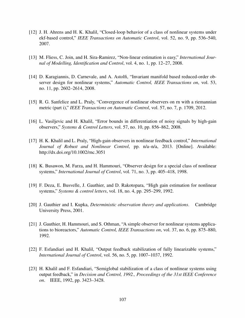
[12] J. H. Ahrens and H. K. Khalil, “Closed-loop behavior of a class of nonlinear systems underekf-based control,” IEEE Transactions on Automatic Control, vol. 52, no. 9, pp. 536–540,2007.

[13] M. Fliess, C. Join, and H. Sira-Ramirez, “Non-linear estimation is easy,” International Jour-nal of Modelling, Identification and Control, vol. 4, no. 1, pp. 12–27, 2008.

[14] D. Karagiannis, D. Carnevale, and A. Astolfi, “Invariant manifold based reduced-order ob-server design for nonlinear systems,” Automatic Control, IEEE Transactions on, vol. 53,no. 11, pp. 2602–2614, 2008.

[15] R. G. Sanfelice and L. Praly, “Convergence of nonlinear observers on rn with a riemannianmetric (part i),” IEEE Transactions on Automatic Control, vol. 57, no. 7, p. 1709, 2012.

[16] L. Vasiljevic and H. Khalil, “Error bounds in differentiation of noisy signals by high-gainobservers,” Systems & Control Letters, vol. 57, no. 10, pp. 856–862, 2008.

[17] H. K. Khalil and L. Praly, “High-gain observers in nonlinear feedback control,” InternationalJournal of Robust and Nonlinear Control, pp. n/a–n/a, 2013. [Online]. Available:http://dx.doi.org/10.1002/rnc.3051

[18] K. Busawon, M. Farza, and H. Hammouri, “Observer design for a special class of nonlinearsystems,” International Journal of Control, vol. 71, no. 3, pp. 405–418, 1998.

[19] F. Deza, E. Busvelle, J. Gauthier, and D. Rakotopara, “High gain estimation for nonlinearsystems,” Systems & control letters, vol. 18, no. 4, pp. 295–299, 1992.

[20] J. Gauthier and I. Kupka, Deterministic observation theory and applications. CambridgeUniversity Press, 2001.

[21] J. Gauthier, H. Hammouri, and S. Othman, “A simple observer for nonlinear systems applica-tions to bioreactors,” Automatic Control, IEEE Transactions on, vol. 37, no. 6, pp. 875–880,1992.

[22] F. Esfandiari and H. Khalil, “Output feedback stabilization of fully linearizable systems,”International Journal of Control, vol. 56, no. 5, pp. 1007–1037, 1992.

[23] H. Khalil and F. Esfandiari, “Semiglobal stabilization of a class of nonlinear systems usingoutput feedback,” in Decision and Control, 1992., Proceedings of the 31st IEEE Conferenceon. IEEE, 1992, pp. 3423–3428.

107

[24] S. Oh and H. Khalil, “Nonlinear output-feedback tracking using high-gain observer and vari-able structure control,” Automatica, vol. 33, no. 10, pp. 1845–1856, 1997.

[25] A. Memon and H. Khalil, “Full-order high-gain observers for minimum phase nonlinear sys-tems,” in Decision and Control, 2009 held jointly with the 2009 28th Chinese Control Con-ference. CDC/CCC 2009. Proceedings of the 48th IEEE Conference on. IEEE, 2009, pp.6538–6543.

[26] L. Freidovich and H. Khalil, “Performance recovery of feedback-linearization-based de-signs,” Automatic Control, IEEE Transactions on, vol. 53, no. 10, pp. 2324–2334, 2008.

[27] A. Chakrabortty and M. Arcak, “Time-scale separation redesigns for stabilization and per-formance recovery of uncertain nonlinear systems,” Automatica, vol. 45, no. 1, pp. 34–44,2009.

[28] J. Back and H. Shim, “Adding robustness to nominal output-feedback controllers for uncer-tain nonlinear systems: A nonlinear version of disturbance observer,” Automatica, vol. 44,no. 10, pp. 2528–2537, 2008.

[29] L. Freidovich and H. Khalil, “Logic-based switching for robust control of minimum-phasenonlinear systems,” Systems & control letters, vol. 54, no. 8, pp. 713–727, 2005.

[30] ——, “Lyapunov-based switching control of nonlinear systems using high-gain observers,”Automatica, vol. 43, no. 1, pp. 150–157, 2007.

[31] S. Nazrulla and H. Khalil, “Robust stabilization of non-minimum phase nonlinear systems us-ing extended high-gain observers,” Automatic Control, IEEE Transactions on, vol. 56, no. 4,pp. 802–813, 2011.

[32] D. Karagiannis, A. Astolfi, and R. Ortega, “Two results for adaptive output feedback stabi-lization of nonlinear systems,” Automatica, vol. 39, no. 5, pp. 857–866, 2003.

[33] Y. Shtessel, S. Baev, C. Edwards, and S. Spurgeon, “Hosm observer for a class of non-minimum phase causal nonlinear mimo systems,” Automatic Control, IEEE Transactions on,vol. 55, no. 2, pp. 543–548, 2010.

[34] A. Teel and L. Praly, “Global stabilizability and observability imply semi-global stabilizabil-ity by output feedback,” Systems & Control Letters, vol. 22, no. 5, pp. 313–325, 1994.

[35] A. Atassi and H. Khalil, “A separation principle for the stabilization of a class of nonlinearsystems,” Automatic Control, IEEE Transactions on, vol. 44, no. 9, pp. 1672–1687, 1999.

108

[36] L. Praly and M. Arcak, “A relaxed condition for stability of nonlinear observer-based con-trollers,” Systems & control letters, vol. 53, no. 3, pp. 311–320, 2004.

[37] A. Isidori, “A tool for semi-global stabilization of uncertain non-minimum-phase nonlinearsystems via output feedback,” Automatic Control, IEEE Transactions on, vol. 45, no. 10, pp.1817–1827, 2000.

[38] V. Andrieu and L. Praly, “Global asymptotic stabilization for nonminimum phase nonlinearsystems admitting a strict normal form,” Automatic Control, IEEE Transactions on, vol. 53,no. 5, pp. 1120–1132, 2008.

[39] D. Karagiannis, Z. Jiang, R. Ortega, and A. Astolfi, “Output-feedback stabilization of a classof uncertain non-minimum-phase nonlinear systems,” Automatica, vol. 41, no. 9, pp. 1609–1615, 2005.

[40] R. Marino and P. Tomei, “A class of globally output feedback stabilizable nonlinear non-minimum phase systems,” Automatic Control, IEEE Transactions on, vol. 50, no. 12, pp.2097–2101, 2005.

[41] S. Hoseini, M. Farrokhi, and A. Koshkouei, “Adaptive neural network output feedback stabi-lization of nonlinear non-minimum phase systems,” International journal of adaptive controland signal processing, vol. 24, no. 1, pp. 65–82, 2010.

[42] A. Gelb, Applied Optimal Estimation. MIT Press, 1974.

[43] H. Soresnson, “Guest editorial: On applications of kalman filtering,” IEEE Transactions onAutomatic Control, vol. AC-28, no. 3, pp. 254–255, 1983.

[44] K. Reif, F. Sonnemann, and R. Unbehauen, “An ekf-based nonlinear observer with a pre-scribed degree of stability,” Automatica, vol. 34, no. 9, pp. 1119–1123, 1998.

[45] K. Reif and R. Unbehauen, “The extended kalman filter as an exponential observer for non-linear systems,” Signal Processing, IEEE Transactions on, vol. 47, no. 8, pp. 2324–2328,1999.

[46] M. Boutayeb and D. Aubry, “A strong tracking extended kalman observer for nonlineardiscrete-time systems,” Automatic Control, IEEE Transactions on, vol. 44, no. 8, pp. 1550–1556, 1999.

[47] M. Boutayeb, H. Rafaralahy, and M. Darouach, “Convergence analysis of the extendedkalman filter used as an observer for nonlinear deterministic discrete-time systems,” Auto-matic Control, IEEE Transactions on, vol. 42, no. 4, pp. 581–586, 1997.

109

[48] P. Moraal and J. Grizzle, “Observer design for nonlinear systems with discrete-time measure-ments,” Automatic Control, IEEE Transactions on, vol. 40, no. 3, pp. 395–404, 1995.

[49] H. Hammouri and J. de Leon Morales, “Observer synthesis for state-affine systems,” in De-cision and Control, 1990., Proceedings of the 29th IEEE Conference on. IEEE, 1990, pp.784–785.

[50] L. Praly and I. Kanellakopoulos, “Output feedback asymptotic stabilization for triangularsystems linear in the unmeasured state components,” in Decision and Control, 2000. Pro-ceedings of the 39th IEEE Conference on, vol. 3. IEEE, 2000, pp. 2466–2471.

[51] G. Besancon, J. De Leon-Morales, and O. Huerta-Guevara, “On adaptive observers for stateaffine systems,” International journal of Control, vol. 79, no. 06, pp. 581–591, 2006.

[52] R. Bucy and P. Joseph, Filtering for stochastic processes with applications to guidance.American Mathematical Society, 1987, vol. 326.

[53] L. Torres, G. Besancon, and D. Georges, “Ekf-like observer with stability for a class of non-linear systems,” Automatic Control, IEEE Transactions on, vol. 57, no. 6, pp. 1570–1574,2012.

[54] N. Boizot, E. Busvelle, and J. Gauthier, “An adaptive high-gain observer for nonlinear sys-tems,” Automatica, vol. 46, no. 9, pp. 1483–1488, 2010.

[55] A. Krener, “The convergence of the extended kalman filter,” Directions in mathematical sys-tems theory and optimization, pp. 173–182, 2003.

[56] A. Isidori, Nonlinear control systems. Springer-Verlag New York, Inc., 1997.

[57] ——, Nonlinear control systems II. Springer Verlag, 1999, vol. 2.

[58] J. Baras, A. Bensoussan, and M. James, “Dynamic observers as asymptotic limits of recursivefilters: Special cases,” SIAM Journal on Applied Mathematics, vol. 48, no. 5, pp. 1147–1158,1988.

[59] M. Pai, Power system stability: Analysis by the direct method of Lyapunov. North-HollandPublishing Company, 1981, vol. 3.

[60] C. Wan, D. Bernstein, and V. Coppola, “Global stabilization of the oscillating eccentric rotor,”Nonlinear Dynamics, vol. 10, no. 1, pp. 49–62, 1996.

110

[61] H. K. Khalil, Nonlinear systems. Prentice hall Upper Saddle River, 2002, vol. 3.

[62] J. G. Kassakian, M. F. Schlecht, and G. C. Verghese, Principles of power electronics.Addison-Wesley Reading, USA, 1991, vol. 46.

[63] A. Astolfi, D. Karagiannis, and R. Ortega, Nonlinear and adaptive control with applications.Springer, 2008.

[64] H. Rodriguez, R. Ortega, G. Escobar, and N. Barabanov, “A robustly stable output feedbacksaturated controller for the boost dc-to-dc converter,” Systems & control letters, vol. 40, no. 1,pp. 1–8, 2000.

[65] R. S. Bucy and P. D. Joseph, “Filtering for stochastic processes with applications to guid-ance,” 1968.

[66] A. N. Atassi and H. Khalil, “A separation principle for the control of a class of nonlinearsystems,” Automatic Control, IEEE Transactions on, vol. 46, no. 5, pp. 742–746, 2001.

[67] M. W. Spong, “Modeling and control of elastic joint robots,” ASME J. Dyn. Syst. Meas.Control, vol. 109, pp. 310–319, 1990.

[68] M. W. Spong and M. Vidyasagar, Robot dynamics and control. Wiley.com, 2008.

[69] M. Benosman and G. Le Vey, “Control of flexible manipulators: A survey,” Robotica, vol. 22,no. 5, pp. 533–545, 2004.

[70] S. K. Dwivedy and P. Eberhard, “Dynamic analysis of flexible manipulators, a literaturereview,” Mechanism and Machine Theory, vol. 41, no. 7, pp. 749–777, 2006.

[71] S. Nicosia and P. Tomei, “A tracking controller for flexible joint robots using only link posi-tion feedback,” Automatic Control, IEEE Transactions on, vol. 40, no. 5, pp. 885–890, 1995.

[72] W. Chatlatanagulchai, H. C. Nho, and P. H. Meckl, “Robust observer backstepping neuralnetwork control of flexible-joint manipulator,” in American Control Conference, 2004. Pro-ceedings of the 2004, vol. 6. IEEE, 2004, pp. 5250–5255.

[73] K. Melhem and W. Wang, “Global output tracking control of flexible joint robots via factor-ization of the manipulator mass matrix,” Robotics, IEEE Transactions on, vol. 25, no. 2, pp.428–437, 2009.

111

[74] S. J. Yoo, J. B. Park, and Y. H. Choi, “Output feedback dynamic surface control of flexible-joint robots,” International Journal of Control Automation and Systems, vol. 6, no. 2, p. 223,2008.

[75] S. Ulrich and J. Z. Sasiadek, “Extended kalman filtering for flexible joint space robot control,”in American Control Conference (ACC), 2011. IEEE, 2011, pp. 1021–1026.

[76] R. Ortega, R. Kelly, and A. Loria, “A class of output feedback globally stabilizing controllersfor flexible joints robots,” Robotics and Automation, IEEE Transactions on, vol. 11, no. 5,pp. 766–770, 1995.

[77] I. Burkov and L. B. Freidovich, “Stabilization of the position of a lagrangian system withelastic elements and bounded control, with and without measurement of velocities,” Journalof applied mathematics and mechanics, vol. 61, no. 3, pp. 433–441, 1997.

[78] A. Ailon, “Output controllers based on iterative schemes for set-point regulation of uncertainflexible-joint robot models,” Automatica, vol. 32, no. 10, pp. 1455–1461, 1996.

[79] B. Brogliato, R. Ortega, and R. Lozano, “Global tracking controllers for flexible-joint manip-ulators: a comparative study,” Automatica, vol. 31, no. 7, pp. 941–956, 1995.

[80] S. Liu, P. Garimella, and B. Yao, “Adaptive robust precision motion control of a flexiblesystem with unmatched model uncertainties,” in American Control Conference, 2005. Pro-ceedings of the 2005. IEEE, 2005, pp. 750–755.

[81] B. Wie and D. S. Bernstein, “Benchmark problems for robust control design,” Journal ofGuidance, Control, and Dynamics, vol. 15, no. 5, pp. 1057–1059, 1992.

112