Estimating the Impact of the Death Penalty on Murderwebs.wofford.edu/pechwj/Estimating the Impact of the Death Penalty... · Estimating the Impact of the Death Penalty on Murder John

Estimating the Impact of the Death Penaltyon Murder

John J. Donohue, III, Yale Law School, and Justin Wolfers, The WhartonSchool, University of Pennsylvania

This paper reviews the econometric issues in efforts to estimate the impact of the

death penalty on murder, focusing on six recent studies published since 2003. We

highlight the large number of choices that must be made when specifying the various

panel data models that have been used to address this question. There is little clarity

about the knowledge potential murderers have concerning the risk of execution: are

they influenced by the passage of a death penalty statute, the number of executions

in a state, the proportion of murders in a state that leads to an execution, and details

about the limited types of murders that are potentially susceptible to a sentence of

death? If an execution rate is a viable proxy, should it be calculated using the ratio

of last year’s executions to last year’s murders, last year’s executions to the murders

a number of years earlier, or some other values? We illustrate how sensitive various

estimates are to these choices. Importantly, the most up-to-date OLS panel data studies

generate no evidence of a deterrent effect, while three 2SLS studies purport to find such

evidence. The 2SLS studies, none of which shows results that are robust to clustering

their standard errors, are unconvincing because they all use a problematic structure

based on poorly measured and theoretically inappropriate pseudo-probabilities that are

The authors gratefully acknowledge the helpful comments received from David Bjerk,Adam Hirsch, Christine Jolls, Ilyana Kuziemko, John Pepper, an anonymous referee, andworkshop participants at the University of Chicago Law School; and the outstandingresearch assistance of Abhay Aneja, Sascha Becker, Chris Griffin, Tatiana Neumann,Wen Yang Qi, and Alexandria Zhang. We thank Tomislav Kovandzic for generouslysharing data that we employed in this study, and Yale Law School for research support.

Send correspondence to: John J. Donohue, Yale Law School, PO Box 208215, NewHaven, CT 06520-8215; E-mail: [email protected].

American Law and Economics Reviewdoi:10.1093/aler/ahp024

C© The Author 2009. Published by Oxford University Press on behalf of the American Law and EconomicsAssociation. All rights reserved. For permissions, please e-mail: [email protected].

1

American Law and Economics Review Advance Access published December 25, 2009 at W

offord College on M

arch 9, 2015http://aler.oxfordjournals.org/

Dow

nloaded from

http://aler.oxfordjournals.org/

2 American Law and Economics Review 2009 (1–61)

designed to capture the key deterrence elements of a state’s death penalty regime, and

because their instruments are of dubious validity. We also discuss the appropriateness

of the implicit assumption of the 2SLS studies that OLS estimates of the impact of the

death penalty would be biased against a finding of deterrence.

Does the death penalty provide greater deterrence of murders beyond thatafforded by a sentence of life imprisonment? This question has been ac-tively debated for centuries, with those arguing that capital punishment isa more severe punishment that will provide greater deterrence opposed bythose who argue that state-sanctioned executions provide an environmentconducive to unsanctioned homicides. Alternatively, some have argued thatthe death penalty is not as dreadful to potential murderers as the thoughtof life imprisonment or that the death penalty is less cost-effective thanits alternatives. In the past half-century, this debate has turned from socialtheorists to empiricists.

Given the availability of relatively high-quality data on American murderrates, executions, criminal justice statistics, and other relevant control vari-ables as well as the number of researchers conducting sophisticated econo-metric studies over the last thirty years, one would think that a consensuswould have emerged about the answer to this ostensibly simple question.Indeed, some believe that it has.

Radelet and Akers (1996) surveyed seventy past presidents of the aca-demic criminology associations asking them “on the basis of their knowledgeof the literature and research in criminology” (Rubin, 2006b) whether thedeath penalty lowered the murder rate. Only eight of these eminent criminol-ogists responded affirmatively to the statement that “the death penalty actsas a deterrent to the commitment of murder—that it lowers the murder rate,”while fifty-six (or 84%) argued against deterrence. (Three past presidentshad no opinion, while a further three failed to respond to the survey.) Radeletand Lacock (2009) administered this same survey in 2008 to an updated listof top criminologists (not including those included in the 1996 survey),and generated similar results: 88% of the seventy-six respondents thoughtthere was no deterrent effect of the death penalty. Dieter (1995) surveyed anationally representative sample of U.S. police chiefs and county sheriffs,finding only 26% found the statement that the “death penalty significantlyreduces [the] number of homicides” to be accurate, while 67% believed itto be inaccurate (7% were unsure).

at Wofford C

ollege on March 9, 2015

http://aler.oxfordjournals.org/D

ownloaded from


Estimating the Impact of the Death Penalty on Murder 3

Yet Becker (2006) argued that “the preponderance of the evidence doesindicate that capital punishment deters.” Joanna Shepherd’s 2004 con-gressional testimony concurred: “In the economics literature in the pastdecade . . . there is a very strong consensus . . . all of the modern economicstudies in the past decades have found a deterrent effect.” Paul Rubin (2006)echoed this assessment before the Senate Judiciary Committee claimingthat “The literature is easy to summarize: almost all modern studies and allthe refereed studies find a significant deterrent effect of capital punishment.Only one study questions these results.”

We provide the emphasis in the Rubin quote because the reference to“one study” is to Donohue and Wolfers (2005), hereinafter “DW”—our ownrather critical response to recent death penalty research published in theStanford Law Review in December 2005. In that paper we evaluated manyof the death penalty studies that Rubin deemed to establish the deterrenteffect of the death penalty. In each case the foundation for these claimsproved to be quite shaky, albeit for varying reasons, including coding errors,inappropriate study designs, improper calculation of standard errors, andreliance on invalid instrumental variables.

Our aim in this paper is not to provide a single “best” estimate of theimpact of the death penalty on murder, but rather to provide a systematicreview of the issues confronting researchers working on this question, as wellas to review the state of the recent and growing literature on the deterrencequestion. Section 1 provides an overview of the history of the econometricdebate on the deterrent effect of the death penalty, briefly summarizing themethodologies and conclusions of some of the major studies evaluating theimpact of the death penalty. Section 2 looks at New York State’s experimentwith capital punishment, which lasted from 1995 to 2004, as a way toillustrate some of the modeling complexities that must be addressed intrying to estimate the impact of capital punishment on murder. Perhapssurprisingly, the two counties in New York City (Manhattan and the Bronx)with District Attorneys (DAs) who strongly and vociferously opposed thedeath penalty experienced the largest drops in murders.

Section 3 illustrates that OLS estimates of the impact of executions onmurder during the post-moratorium period (post-1976) consistently showno statistically significant evidence of deterrence, while Section 4 notesthat a number of studies find greater evidence of deterrence using instru-mental variables techniques. Unfortunately, the 2SLS studies have some

at Wofford C



ownloaded from



major flaws. First, they all use a problematic structure based on poorly mea-sured and theoretically inappropriate pseudo-probabilities that are designedto capture the key deterrence elements of a state’s death penalty regime.Second, their estimated deterrence effects are statistically insignificant ifclustering the standard errors is necessary. Third, since researchers haveisolated few credible sources of exogenous variation in execution policy,there is little reason to credit 2SLS estimates that rest on such flawed in-struments. Section 5 goes on to analyze the issue of possible endogeneitybias in the OLS estimates, and argues that in the post-moratorium periodthat bias may well operate in favor of deterrence. If so, then 2SLS estimatesthat find a stronger deterrent effect than that of the OLS estimates—whichis the case in the studies by Dezhbakhsh et al. (2003) (hereinafter “DRS”),Mocan and Gittings (2003) (hereinafter “MG”) and Zimmerman (2004)—are presumptively invalid.

Section 6 offers concluding remarks and notes that if the 2SLS studiesare unreliable and the OLS studies provide an upper-bound estimate of theimpact of the death penalty, then the absence of any statistically significanteffect in the OLS estimates presents a major challenge to those arguing for a“strong deterrent” of capital punishment. Of course, there is a fundamentaldifficulty in teasing out the impact of the death penalty in post-moratoriumperiod in the United States in that there may not have been sufficient variationacross states in execution policy to yield precise estimates of the relationshipbetween capital punishment and homicide.

But recent evidence from the massive increase, and then subsequentdecline, in executions in Singapore suggests that potential murderers tendnot to be responsive to levels of execution that are dramatically higher thanthose in modern day Texas. Indeed, the time path of homicide in Hong Konglooks strikingly similar to that of Singapore even though the former neverused capital punishment and formally abolished it shortly before Singaporebegan its experiment in extremely heavy reliance on the death penalty.

1. Some History of the Econometric Debate

1.1. The Pioneering, but Now Superseded, Early Work

In 1975, Isaac Ehrlich developed a sophisticated econometric modelusing national time-series data and claimed to show that each execution

at Wofford C



ownloaded from



between 1933 and 1969 saved eight lives. Although Ehrlich merits credit asan original and innovative contributor to an important conceptual literatureon the economics of deterrence, his paper precedes the major advances inmicro-econometric evaluation of panel data. Specifically, a national time-series analysis is incapable of providing robust empirical estimates of theimpact of the death penalty because it cannot identify whether any changesin murder rates are occurring in the states that invoke capital punishment.Indeed, the national time-series approach can only yield a valid estimatein the unlikely event that two conditions hold: (i) the rate of executions isorthogonal to the large, unexplained movements in the murder rate overtime; and (ii) an execution anywhere in the United States is equally likelyto deter a murder throughout the United States (even in jurisdictions thathave no death penalty) or the unexplained differences in murder rates acrossdifferent jurisdictions are constant over time.1

In response to criticisms of his time-series approach, Ehrlich produced asecond cross-sectional study in 1977 that looked at murder rates and execu-tions across states in two years—1940 and 1950. But it is now recognizedthat cross-sectional studies are even less suited for estimating the causalimpact of executions because they cannot easily account for the large andpersistent, unexplained differences in crime rates across states. Specifically,the cross-sectional analysis cannot address the unobserved heterogeneitythat underlies the fact that in the United States murder rates tend to be sub-stantially lower in nonexecuting states than in high execution states, as theregional breakdown in Table 1 suggests. Clearly, there are reasons why, say,Maine with a 2004 murder rate of 1.4 per 100,000 is safer than Mississippi,where the murder rate of 7.8 is more than five times as high, but fully

1. A particularly telling problem with the Ehrlich time-series analysis was that hisfinding of a deterrent effect emerged only because Ehrlich used a log specification thatgave disproportionate weight to the fact that the small reduction in the execution rate froma very low level to virtually zero in the late 1960s was accompanied by a very large jump inmurders. Stopping the analysis in 1962 rather than 1969 or using a nonlogarithmic modelwould generate no deterrent effect. This nonfinding seems more intuitively plausible inthat the 80% decline in the execution rate over the period of 1933–1962 occurred duringa period of falling murder rates (from 8.8 per 100,000 to 4.6, a decline of 47.7%) and thelarge post-1962 increase in murder rates occurred identically in states that never had thedeath penalty as well as those that did. See Figure 3 in DW. Numerous other conceptualand data problems with Ehrlich’s work are discussed in Section 4.1 and in the Appendix.

at Wofford C



ownloaded from



Table 1. Homicide and Execution Rates by Region: 2002

Region Homicide rate (per 100,000) Execution rate (per 100,000)

Northeast 4.1 0.0Midwest 5.1 0.014West 5.7 0.002South 6.8 0.059

explaining these enduring differences without the benefit of a state fixed-effect dummy has proven to be a daunting challenge.

By the time various scholars—backed up by a 1978 National Academy ofSciences report—were done pointing out the infirmities in Ehrlich’s analy-sis, few outside of the University of Chicago believed that either his nationaltime-series analysis or his cross-sectional analysis afforded substantial sup-port for the view that each additional execution saves many lives.2

1.2. The Move to Panel Data

It is now widely recognized that panel data models with state and yearfixed effects, while hardly foolproof, are far more likely to identify the causalimpact of a legal or policy change, such as the death penalty, than time-seriesor cross-section models (Nerlove, 2002). As we will see, the difficulties intrying to reliably estimate the impact of the death penalty using the besttools are daunting enough; there is really no hope that we can do so usingless reliable statistical methodologies, such as time-series and cross-sectionstudies. Unfortunately, not everyone has gotten this message. While suchpapers continue to be published, they likely should be ignored.3 For thisreason, we limit our attention to the issues involved in the specification

2. Cameron (1994) provides a detailed review of the pre-“panel data” literature byEhrlich, his critics, and other scholars using time-series or cross-section approach. Heconcludes that “the presence of capital punishment on the statute book acts as some kindof deterrent but variations in its use do not.” Interestingly, Ekelund et al. (2006) findsthat the presence of a death penalty statute increases murder but higher use dampens thisincrease.

3. Ehrlich and Liu (1999) and Liu (2004) (both using Ehrlich’s original state-level,cross-section data from 1940 and 1950) and Narayan and Smyth (2006) (using national-level time-series data for 1965–2001) may offer insights about innovations in these moreprimitive statistical tools, but, given the now extensive panel data analyses, these less-discerning approaches cannot be expected to advance our understanding of the causalimpact of the death penalty on murder.

at Wofford C



ownloaded from



and estimation of panel data models, and to one new matching study thatcompares high-execution Singapore with abolitionist Hong Kong.

John Lott and David Mustard created a panel dataset beginning with 1977data (for use in their evaluation of state right-to-carry concealed handgunlaws) that greatly influenced a new round of estimates of the impact ofthe death penalty on crime.4 Lott and Mustard essentially followed theEhrlich model and then shared their state and county data with a number ofresearchers, who used it to analyze the death penalty: MG and Zimmerman(2004) conducted their analyses on state data using both OLS and 2SLSmethods, and DRS relied on 2SLS estimation on county data to offer supportfor the view that the death penalty deters murder.5 Unfortunately, this piggy-back approach has meant that some of the conceptual errors of Ehrlich havepersisted over time, and some of the data and specification problems thatwere introduced in the original Lott and Mustard dataset have infectedsubsequent papers that have used their data.6

At the same time, another major state panel data study by Katz et al.(2003) using OLS estimation concluded that there was little empirical

4. The 1977 date was mandated by Lott and Mustard’s desire to use arrest rate data,which became available by county in that year. While Lott and Mustard were followingEhrlich’s lead in using arrest rates as an explanatory variable in their crime model, theproblems with using this variable are discussed in Section 4.1.

5. Section 4.1 describes some general inadequacies in Ehrlich’s theoretical andeconometric specification that have carried over to the models employed by DRS, MG,and Zimmerman. MG relied primarily on an OLS panel data regression, but also presentedone table of 2SLS estimates, which we critique in Section 4.2.2. The OLS estimates inboth Zimmerman (2004) and Zimmerman (this issue) do not indicate that capital pun-ishment deters (that is, the explanatory variable “executions/death sentences” measuredcontemporaneously or lagged one year was negative but not statistically significant).

6. The DRS dataset, which came from Lott and Mustard, contains demographicvariables that provide the percentages of county population of the following age groups:ages 0–9, 10–19, 20–29, 30–39, 40–49, 50–64, and 65 and over; race groups: black,white, and other; and sex groups: male and female. After summing these variables withingroups, we find that the minimum values for total age, total race, and total sex are 99.97%,99.97%, and 70.56%, respectively, which suggests something has gone quite wrong in thesex breakdown. The maximum values for total age, total race, and total sex are 132.67%,105.76%, and 156.66%, respectively. Clearly, the age groups, race groups, and sex groupsdo not sum up to 100% for all counties over all years. Most notably, the sum of femaleand male population percentages falls below 90% for nearly 80% of the observations (thispercentage excludes observations that would be dropped from the regressions becauseone or more of the demographic variables are missing data, which constitute about 10%of the total number of observations).

at Wofford C



ownloaded from



support for the deterrence hypothesis. These authors use neither the Ehrlichmodel nor the Lott and Mustard data, which means they thereby avoided anumber of serious data and specification problems.

While DW raised substantial concerns about the DRS, MG, and Zimmer-man papers and found the KLS paper more reliable, not everyone agrees:for example, David Muhlhausen of the Heritage Foundation, testifying onJune 27, 2007, before the Subcommittee on the Constitution, Civil Rights,and Property Rights of the Committee on the Judiciary of the United StatesSenate, reviewed the work of Ehrlich and these three pro-deterrence papers:

the recent studies using panel data techniques have confirmed what we learneddecades ago: Capital punishment does, in fact, save lives. Each additionalexecution appears to deter between three and 18 murders.

Muhlhausen’s confident assessment of the recent research was notablein that it ignored both the KLS paper, our own critique of the previouslymentioned studies that Muhlhausen found persuasive, and every other studydisputing a finding of deterrence for capital punishment (some recent onesprior to Mulhuausen’s testimony include Berk, 2005; Fagan, 2006; Faganet al., 2006; some subsequent articles include Zimring, 2008; Cohen-Coleet al., this issue; Hjalmarsson, this issue; Kovandzic et al., 2009). In fact,the only other panel data study that Muhlhausen referenced in his one-sidedreview of the literature was Ekelund et al. (2006), which concluded thatsingle-victim homicides were deterred by capital punishment but multiple-victim homicides were not. Muhlhausen did not mention that one of thestrongest findings in the Ekelund study was that the presence of a capitalpunishment regime led to more homicides, so in our reading, as we explainfurther below, the Ekelund study actually undermines rather than supportsthe deterrent effect of the death penalty.7

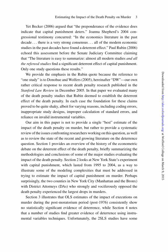
Moreover, the most comprehensive assessment of the impact of the deathpenalty using the latest data—a recent paper by Kovandzic, Vieraitis, andBoots (“KVB”)—has just concluded that there is “no empirical supportfor the argument that the existence or application of the death penalty de-ters prospective offenders from committing homicide.” Table 2 providesa capsule summary of the six panel data studies just mentioned, of which

7. In their meta-analysis of death penalty studies, Yang and Lester (2008) list theEkelund study as showing that capital punishment leads to an increase in homicides.

at Wofford C



ownloaded from


Estim

atingthe

Impactof

theD

eathPenalty

onM

urder9

Table 2. Six Panel Data Studies on Impact of Executions on Murder Rates

(1) (2) (3) (4) (5) (6) (7) (8)Study Geographical

unit of analysis(time period of

analysis)

OriginalOLS

estimates

Corrected orexpanded

OLSestimates

Original2SLS

estimates

Corrected2SLS

estimates andevaluation

Instruments Assessmentof instrument

validity

(1) Dezbakhsh,Rubin,Shepherd(ALER,2003)

County-level(1977–1996)

None Inconsistent—we generatedOLSestimatesbased onoriginal DRSdata andspecificationminus theinstruments.

Negative (stat.significant)

Negative (notsignificant,with clusteredstandarderrors).

(1) Policespending,

(2) Judicialspending,

(3) Prisonadmissions,

(4) % voting for aRepublicanpresident; allinstrumentsare state-level

Not valid

Invalid if theinstrumentsare deemedinvalid (seenext twocolumns).

(continued )

at Wofford College on March 9, 2015 http://aler.oxfordjournals.org/ Downloaded from


10A

merican

Law

andE

conomics

Review

2009(1–61)

Table 2. Continued

(1) (2) (3) (4) (5) (6) (7) (8)Study Geographical

unit of analysis(time period of

analysis)

OriginalOLS

estimates

Corrected orexpanded

OLSestimates

Original2SLS

estimates

Corrected2SLS

estimates andevaluation

Instruments Assessmentof instrument

validity

(2) Mocan andGittings(ALER,2003)

State-level(1984–1997)


Negative andinsig. w/ocoding errors;positive andinsig. usingZimmermanexecutionratio


Negative (notsignificant,with clusteredstandarderrors).

Invalid if theinstrumentsare deemedinvalid (seenext twocolumns).

(1) Deterrencevariables t – 2,

(2) Death penaltylaw t – 1,

(3) Death penaltylaw t – 2

Not valid

(3) Zimmerman(J. Appl.Econ, 2004)


Negative (notsignificant)

Zimmermanreaffirms thisfinding of nosignificancein hiscontributionto this issue


Proportion ofmurderscommitted att and t – 1:

(1) by strangers,(2) with nonfelony

murdercircumstances,and

(3) by non-whiteoffenders;

(4) indicator forrelease fromdeath row att – 1,

(5) indicator for“botchedexecution” att – 1

(1)–(4) notvalid;(5) weak



Estim

atingthe

Impactof

theD

eathPenalty

onM

urder11

(4) Katz, Levitt,andShustorovich(ALER,2003)


Mostly negative(some stat.significant)

We expand thedata to1934–2000;results aremixed(but only stat.significantresults arepositive for1934–1960.)

(5) Ekelund,Jackson,Ressler, andTollison(SouthernEconomicJournal,2006)


Positive for allmurders (stat.significant)

Too short a timeframe to bereliable, andno state fixedeffects

(6) Kovandzic,Vieraitis, andBoots (Crim-inology andPublicPolicy, 2009)


Mostly negative(never stat.significant)

Notes: Corrected estimates are based on Donohue and Wolfers (2005) and this paper. “Negative” estimates imply that each execution deters murder. “Positive” implies the death penaltyregime is linked with an increase in the number of murders. Shading indicates statistical significance.The first three studies offer evidence of deterrence with 2SLS models (and, in the case of Mocan and Gittings, with OLS models). These findings are all suspect for the reasons listed.The fourth study by KLS based on OLS models concludes: “there is little evidence in support of a deterrent effect of capital punishment as presently administered.” A more extensiveexploration in the sixth study by KVB reaches the same conclusion. The Ekelund et al. study purports to show deterrence for single murders and increases in multiple murders, but whencorrectly interpreted shows the death penalty is associated with higher levels of both types of murder. The Ekelund results are likely spurious, owing to the short time frame and the lack ofstate fixed effects.




three provide support for the deterrence hypothesis and three undermine thishypothesis.

With so much conflicting evidence being bandied about (or ignored whenconvenient), and with experts telling Congress that studies support the de-terrent effect of the death penalty when they actually refute that claim, itmay be useful to provide an overall assessment of the latest literature witha view to understanding why different researchers have reached such diver-gent conclusions while frequently relying on the same U.S. homicide data.Hopefully, this paper can give some guidance both to researchers interestedin studying capital punishment and to legislators, policymakers, and aca-demics who may be confused by such conflicting assessments of its likelyimpact on murder.

It will be helpful to provide a brief roadmap to Table 2. One can seefrom the second column whether the particular study used state or countydata (only DRS relied on county data), and what years were analyzed. Notethat of the five studies that examine more than five years of data, only KVBpresent data after 1997 (their dataset runs from 1977 to 2006). The nextcolumn notes that five studies presented OLS estimates, indicating whetherthese estimates are positive (suggesting antideterrence, as in the Ekelund pa-per) or negative (suggesting deterrence, as in MG), with significant findingsidentified by a shaded box. The fourth column provides additional informa-tion or corrections to the original OLS estimates, starting with our effort toprovide OLS estimates drawing on the structure of the 2SLS DRS models(row 1—these are our estimates since DRS did not present OLS estimates),and continuing down to our efforts to correct some MG coding errors, ex-tend the KLS time period, etc. The bottom line of column 4 supports thecolumn 3 finding of KVB that there is no OLS support for a deterrent effectof capital punishment.

The next four columns of Table 2 (columns 5–8) summarize the threestudies that provide 2SLS estimates. Column 5 shows that all three studiespresent negative and significant estimates (suggestive of deterrence), butcolumn 6 indicates that they all become insignificant if one clusters thestandard errors. Column 7 lists the instruments that are employed in thethree studies, and column 8 reveals that in all but one case, the instrumentsare invalid. Of course, invalid instruments cannot be expected to yield validestimates.

at Wofford C



ownloaded from



2. Using New York’s Death Penalty Experiment to IllustrateSome Modeling Complexities

Many complex issues lurk in the background as one tries to specifythe appropriate model for estimating the impact of capital punishment.An example exploring the depth, accuracy, and geographic precision of theinformation available to potential murderers may be instructive. Crime in thelate 1980s and early 1990s rose sharply in New York during the initial crackepidemic and then started to turn down in about 1992. Republican GeorgePataki managed to unseat Mario Cuomo in 1994 in part on the pledge that hewould restore the death penalty to the state, which he succeeded in doing in1995. This New York death penalty statute remained in effect for a decadeuntil it was declared unconstitutional by the highest state court in 2004.New York’s recent dalliance with the death penalty never resulted in anexecution. While politicians and think-tank advocates, such as David Frumof the American Enterprise Institute, have made the unsupported claim thatthe death penalty statute played a substantial role in New York’s renowneddrop in murders (Frum, 2006), the New York experience offers insight intothe modeling choices involved in trying to estimate the true impact of capitalpunishment.

2.1. Endogenous State Adoption of a Death Penalty Statute?

The New York story immediately raises an endogeneity concern: thestate, and indeed the nation, had endured a sharp increase in crime in thelate 1980s and early 1990s, which aided Pataki’s bid to unseat death penaltyopponent Mario Cuomo. (The high national crime rate likely contributedto the 1994 Republican landslide that also defeated Texas Governor AnnRichards, and ushered in a Republican majority to both houses of Congress.)By 1995, of course, the sharp drop in crime was well underway, but thereis a danger that a regression will spuriously attribute to New York’s 1995death penalty law this mean reversion in the level of crime. Before tryingto assess the best approach to modeling the elements of the death penaltyto which potential murderers might respond, note that these choices canbe influential in estimating the impact of capital punishment: New York’svery substantial murder rate decline continued after 1995, and, since all ofthe Table 2 regression studies weight by population, whether New York iscounted as a treatment state (based on its 1995 law) or a control (based on its

at Wofford C



ownloaded from



lack of executions) can be important. Obviously, if one models New York’sunusually large post-1995 murder rate decline as being influenced by thedeath penalty, then the deterrence argument will be strengthened.

2.2. What Do Potential Murderers Know?

The standard economic model assumes that individuals respond to prices,which they are able to estimate with reasonable precision. For consumerpurchases, price information is readily available, and the cost must be paidwith certainty if the product is to be obtained. In such cases, prices can enterthe demand equation, and there is no need to introduce the complexities ofpsychological or information factors.

In the case of the death penalty, however, there is considerable uncertaintyabout the expected risk of execution. The econometrician needs to employa proxy for this expected risk that captures the information available to andrelied upon by potential murderers. For example, would potential capitalmurderers be aware of the presence of the New York death penalty statute(and therefore be deterred when the law took effect) or would they onlylearn of the law when, or fail to credit the possible sanction until, deathsentences were handed out or convicts were executed? If passage of the lawwith great fanfare—recall that this was a major part of Pataki’s successfulgubernatorial campaign—discouraged criminals from committing murder,then a binary identifier of the state legal capital punishment regime (the lawdummy approach) would be appropriate.

But how much else do potential killers know? Would they know thatcertain county prosecutors in New York opposed the death penalty, renderingthe risk of execution in those areas virtually zero? Specifically, ManhattanDistrict Attorney Robert Morganthau and Bronx District Attorney RobertJohnson were adamantly opposed to the death penalty, and made their viewquite clear before the death penalty law took effect. Writing in the New YorkTimes in February 1995, Morganthau stated:

People concerned about the escalating fear of violence, as I am, may believethat capital punishment is a good way to combat that trend. Take it fromsomeone who has spent a career in Federal and state law enforcement, enactingthe death penalty in New York State would be a grave mistake.

Prosecutors must reveal the dirty little secret they too often share only amongthemselves: The death penalty actually hinders the fight against crime.

at Wofford C



ownloaded from



. . . It exacts a terrible price in dollars, lives and human decency. Rather thantamping down the flames of violence, it fuels them while draining millions ofdollars from more promising efforts to restore safety to our lives.

Some crimes are so depraved that execution might seem just. But even in theimpossible event that a statute could be written and applied so wisely that itwould reach only those cases, the price would still be too high.

It has long been argued, with statistical support, that by their brutalizing anddehumanizing effect on society, executions cause more murders than theyprevent. “After every instance in which the law violates the sanctity of humanlife, that life is held less sacred by the community among whom the outrageis perpetrated.”

Despite Morganthau’s pleas, New York State went on to adopt a deathpenalty statute shortly thereafter. As a judge from New York’s highest courtlater noted:

The very same day the legislation was signed into law by the Governor, theBronx County District Attorney issued a press release purporting to “make[his] policy clear regarding the exercise of [his] discretion” to impose thedeath penalty. In this statement, the District Attorney expressed deeply feltconcerns regarding the effectiveness and administration of the death penalty.He concluded by stating, ‘For all these reasons, while I will exercise mydiscretion to aggressively pursue life without parole in every appropriatecase, it is my present intention not to utilize the death penalty provisions ofthe statute.’ On November 2, 1995, the District Attorney was reelected byapproximately 89% of Bronx County citizens who voted. Johnson v. Pataki,91 N.Y.2d 214, 691 N.E.2d 1002, 668 N.Y.S.2d 978 (1997), Smith, Judge(dissenting).

Despite this articulated opposition to the death penalty, from 1995 to 2004the murder rate dropped in Manhattan by 64.4% (from 16.3 to 5.8 murdersper 100,000), and in the Bronx by 63.9% (from 25.1 to 9.1 per 100,000).8

Another New York City borough with the identical laws and police force,and with broadly similar economic, social, and demographic features asManhattan and the Bronx—Brooklyn—had a top prosecutor who issued thelargest number of notices of intention to seek the death penalty (albeit withno executions) (Kuziemko, 2006). Yet Brooklyn experienced only a 43.3%

8. In the rest of New York State (excluding Manhattan and the Bronx), the murderrate fell by only 36.5% (from 6.5% to 4.1%).

at Wofford C



ownloaded from



decline in murders over this period, from an initial figure (almost identicalto Manhattan’s) of 16.6 murders per 100,000 in 1995 down to only 9.4 in2004. Just as Frum’s claim that New York’s murder drop resulted from thepassage of the death penalty law in 1995 is unfounded, one cannot drawstrong causal inferences from the fact that Manhattan and the Bronx led theway in the decline in homicides, but certainly, there is not even a hint ofa deterrent effect of capital punishment in the crime patterns across thesecounties with anti-death-penalty prosecutors.

For our purposes, the important points are the modeling complexities:Was any of the two-thirds drop in the Manhattan and Bronx murder rates theresult of New York’s death penalty law, or did potential murderers understandand rely upon the anti-death-penalty pronouncements of the DAs in bothcounties? As the next subsection shows, these complexities are often sweptunder the rug by certain specification choices.

2.3. The Law Dummy Model

Table 2 focuses on studies that have modeled the impact of the deathpenalty with a variable that in some form counts the number of executionsin a given state and year. It is possible, though, that the simple presenceof a state law authorizing capital punishment is enough to deter. Considertwo panel data studies that have sought to test this proposition by runninga regression with a “law dummy” indicating the presence of a capital pun-ishment law. First, using data for 1960–2000, Dezhbakhsh and Shepherd(2006) reported that the coefficient on the law dummy was negative (that is,finding deterrence) and statistically significant. DW showed, however, thatthis result became insignificant when the standard errors were adjusted byclustering and when year fixed effects were added to the regression (as isstandard) (see Table 2 of Donohue and Wolfers, 2005).

Second, as indicated in the first column of Table 3, MG find that deathpenalty laws have had a statistically significant dampening effect on mur-der, using the 1977–1997 data. While, as Section 3.2 below reveals, DWestablished that the MG OLS results claiming executions lead to fewermurders go away if MG’s coding errors are corrected, this same correc-tion had only a small dampening effect on the negative and statisticallysignificant estimate that MG present in their death penalty indicator model(compare column 1 to column 2 in Table 3). But Table 3 illustrates the impor-tance of New York to MG’s apparent deterrence conclusion, since dropping

at Wofford C



ownloaded from



Table 3. Impact of Legalized Death Penalty: Testing the Sensitivity of Mocanand Gittings’ Results (1977–1997)

(1) (2) (3) (4)Original MG Corrected NY observations NY death penalty

estimates estimates dropped indicator set to 0

Death penalty legal −0.154∗∗ −0.151∗∗ −0.0021 −0.0018Indicator (t – 1) (0.0061) (0.0063) (0.0048) (0.0073)

Notes: Standard errors are robust and clustered at the state level. Corrected estimates based on the discussion inDonohue and Wolfers (2005). ∗∗ indicates statistical significance at the 0.05 level.While MG’s estimate of the impact of a valid death penalty law is negative and significant (column 1), evenwhen corrected for coding errors (column 2), these results are entirely dependent on the state of New York. IfNew York state is simply dropped from the analysis (column 3), the coefficient drops by two orders of magnitudeand becomes insignificant. Column 4 yields results similar to column 3 when New York is treated as not havinga death penalty law (the state never executed anyone during or after this sample period, the DAs in Manhattanand the Bronx, which enjoyed enormous drops in crime over this period, were staunch opponents of capitalpunishment, and the law was ultimately ruled unconstitutional).

New York decreases the estimate by two orders of magnitude and eliminatesthe finding of statistical significance (column 3). Column 4 shows virtu-ally the same result as column 3 if we code the New York legal dummy aszero for the years 1995–1997 (in essence, positing that potential murdererscorrectly realized that there was virtually no risk of execution in New Yorkdespite the passage of the statute). In other words, the big drop in murders inNew York in the mid-1990s, led by Manhattan and the Bronx, whose DAsstrongly articulated opposition to the death penalty, is what drives the findingthat the presence of a death penalty law is correlated with lower crime.

Finally, KVB has run the dummy variable model on the longest timeperiod of 1977–2006 and has found that the death penalty is never significantat the 0.05 level, although it is significant at the 0.10 level if clustering isnot needed (again attributing the New York decline in murders from 1995to 2004 to the death penalty law).

3. OLS Estimates of the Impact of Executions on Murder

We now turn to the Table 2 studies that model the impact of capitalpunishment with some measure of the frequency of executions. The tableimmediately reveals the key methodological difference between the threestudies that support the deterrence hypothesis and the three that do not: onlythe studies that present 2SLS estimates—DRS, MG, and Zimmerman—claim to find deterrence, while the studies that rely only on OLS—KLS,

at Wofford C



ownloaded from



Ekelund et al., and KVB—show no evidence of deterrence. The secondcolumn of Table 2 summarizes the OLS results provided in five of the sixstudies (DRS did not show OLS results). Column 3 shows that after correc-tion or expansion of the data period, there is no support for the deterrencehypothesis in the OLS estimates across any of the six studies. We discussthe OLS results of the six studies in turn.

3.1. Dezhbakhsh, Rubin, and Shepherd—DRS

DRS did not present OLS results, instead relying on a 2SLS approachthat we discuss in greater detail in Section 4. Using DRS data and specifica-tions but without instrumenting, we obtained OLS estimates of the impactof executions on murder rates. The results were unstable and inconsistent.Specifically, for DRS’s six models, we generate one OLS estimate that isstatistically significant and positive (antideterrent) and two that are signif-icant and negative (deterrent). The other three estimates are negative butinsignificant.9

Even if these results were not conflicting, there would be little reason tocredit them in light of the fact that the DRS specification (that is, their 2SLSestimation, which we converted into an OLS estimation) does not controlfor either the number of police or the extent of incarceration in assessingthe impact of executions on murder, even though a vast literature suggeststhat more police and higher levels of incarceration reduce the murder rate.This choice is particularly problematic given the fact that Texas enjoyed anextremely sharp drop in crime in part because of an enormous increase inincarceration, which coincided with the increase in executions. In general,any empirical study of murder that does not control for the incarcerationrate risks suffering from major omitted variable bias, and should not be

9. Table 1 of DW established that the effort by Dezhbakhsh and Shepherd to ex-amine the effect of death penalty abolitions and reinstatements, which purported to showevidence of crime increases from abolition and crime drops from reinstatement, led to nosuch conclusion if one compared the changing states (the treated group) with the controlgroup of nonchangers. DW also showed that the claim by Cloninger and Marchesinithat the Illinois and Texas death penalty moratoria led to an increase in homicide wasthe product of their decision to examine growth rates in homicide. When we replicatedtheir analysis using levels of homicide, the evidence of an unusual jump in murders disap-peared. (Indeed, in Illinois this approach suggested that the moratorium was accompaniedby a statistically significant decline in the murder rate.)

at Wofford C



ownloaded from



Table 4. Reanalyzing MG’s OLS Estimations of the Impact of Executions onthe Murder Rate (1984–1997)

Corrected MG OLS Results

Dependent variable

Murder rate Robbery rate Violent crime rate Burglary rate

Execution (t – 1) −0.50 (0.34) −3.14 (7.71) −4.69 (16.13) 4.60 (19.83)per death sentence (t – 7)

Execution (t – 1) 0.03 (0.14) 5.11 (4.44) 9.81 (11.70) 2.94 (16.06)per death sentence (t – 1)

Notes: Standard errors are robust and clustered on the state level. Basic specifications are from MG. Correctionsto MG’s OLS estimates are outlined in Donohue and Wolfers (2005). MG employed a dummy for Oklahomain 1995 to control for the Oklahoma City bombings and this indicator is not included in the robbery andburglary regressions. While MG achieves a negative (albeit insignificant) coefficient on the execution variablefor the murder rate equation, the fact that similar negative coefficients emerge in the robbery and violent crimeequations suggests that executions are proxying for some other impact dampening violent crime. When wefollow Zimmerman and lag the death sentence only 1 year, the estimated effect on murder becomes positive, asit is for all other crimes (row 2).

relied upon.10 While DRS (like Lott and Mustard in their work on guns)followed the original model of Ehrlich in the unfortunate choice of omittingincarceration as an explanatory variable, the DRS study and the Ekelundstudy are the only two studies in Table 2 marred by this particular flaw.

3.2. Mocan and Gittings—MG

At first glance, the MG paper appears to make a persuasive case for thedeterrence hypothesis. MG finds that executions are linked with statisticallysignificantly lower rates of murder. MG then seek to confirm that the deathpenalty is not simply a proxy for some other anticrime influence by showingthat when their model is run on other crimes, such as robbery, rape, and twoproperty crimes, the effects are no longer statistically significant. (For thetwo property crimes the effect is positive, and for the two violent crimes it isnegative). But DW found that MG’s OLS results were the product of a codingerror (see DW, Table 6). When the coding error is corrected, the statisticallysignificant effect in the MG OLS regressions disappears, as indicated in thefirst column and first row of Table 4.

10. While controlling for incarceration, Moody and Marvell (2009) report that exe-cutions had no statistically significant impact on murder in their county data analysis forthe period 1977 through 2000.

at Wofford C



ownloaded from



Despite the lack of significance, should the negative sign be taken as someevidence of deterrence? Two reasons undermine even this weak conclusion.First, as the first row in Table 4 indicates, MG followed DRS in specifyingthe execution variable as a ratio of executions last year to death sentencesseven years ago (to predict today’s murders). While we find the ratio ofexecutions to death sentences to be an unconvincing explanatory variable(as discussed in Section 4.1), if it is to be used, we agree with Zimmerman’sargument that a better measure would be the ratio of executions to deathsentences lagged one year (since potential criminals will respond to the mostrecent evidence on sanctions). As Table 2 indicates and row 2 of Table 4depicts, when we follow the Zimmerman approach and posit that potentialcriminals would base their decisions about criminal homicide on more recentdata by using the once-lagged ratio of executions to death sentences, the MGmurder coefficient estimate turns positive (yet insignificant), consistent withthe view that the death penalty increases murder (see DW, Table 6, panelC).11

Second, as MG showed and we document in the first row of Table 4,the coefficient on the execution variable generated a similar negative signin “explaining” robbery and violent crime. The similar signs on the ex-ecution variables in these violent crime equations suggest that the deathpenalty is likely proxying for other factors that cause overall violent crimeto fall (or which correlate with such declines).12 Such an effect would beconsistent with our discussion above of omitted variables bias in the DRSstudy. However, when we again follow the Zimmerman approach and lagdeath sentences only by one year, we see that executions positively cor-relate with all crimes, including murder (although nothing is statisticallysignificant—see row 2 of Table 4).

11. When we employ the same lag structure in the DRS 2SLS model, however, theestimates jump in the opposite direction: the coefficient on predicted executions_t – 1/death sentences_t – 1 is significant at the 5% level in the second stage, and the implied livessaved jump from eighteen to an eye-popping eighty-five. Thus, one sees how sensitivethese models are in that identical changes in lag structures lead to very different resultsin different studies.

12. Conceivably, one might argue that the death penalty could have an indirectdampening effect on violent crime, but this would typically not be a traditional argumentbased on the criminal responding to the risk of capital punishment when consideringwhether to commit a crime since no crime other than an aggravated murder would beeligible for the death penalty.

at Wofford C



ownloaded from



3.3. Zimmerman

Zimmerman concluded that none of his OLS estimates of the impactof executions on murder for 1978–1997 reached statistical significance. InZimmerman’s latest work (in this issue), he adds a lagged dependent variableto his model and again computes OLS results for the same time period.He concludes: “the OLS specifications . . . again provided no evidence tosuggest a deterrent effect of capital punishment, which is consistent withZimmerman’s original results.”

3.4. Katz, Levitt, and Shustorovich—KLS

KLS only presented OLS results, which were estimated on state data fromthe period 1950–1990. While the presence of some sporadic statisticallysignificant KLS estimates led Joanna Shepherd and Paul Rubin to testifybefore Congress that the refereed studies unanimously supported the viewthat the death penalty deterred murder, KLS concluded their own study asfollows: “there is little evidence in support of a deterrent effect of capitalpunishment as presently administered.”

An appealing aspect of the KLS study is that it was designed to probewhether prison conditions influenced crime rates and simply used the ex-ecution rate as a control. As a result, there is little reason to fear that theauthors selected their regression approach to make a particular point aboutthe deterrent effect of the death penalty. To see whether the KLS conclusionwould be robust to various modifications and extensions, we added addi-tional years of data going back to 1934 and coming forward through 2000.Table 5 describes the various permutations, starting with a simple expansionof the exact KLS model to extend an additional ten years through 2000. Thisdata expansion eliminated the sporadic statistically significant evidence ofdeterrence noted by Shepherd and Rubin.

The first row of Table 5 shows the particular base model, devised forKLS’s exploration of the impact of prison harshness, as proxied by deathrates in prison. In this row, the impact of executions on murder is estimatedusing a ratio of executions per prisoner in the state’s penal system. The nexttwo panels of Table 5 describe the results when two other specifications of theexecution variable were used: (i) the ratio of executions to lagged murders,and (ii) the ratio of executions to population. Not one of the regressionssummarized in Table 5 showed a statistically significant deterrent effect,

at Wofford C



ownloaded from


22A

merican

Law

andE

conomics

Review

2009(1–61)

Table 5. The Impact of Executions on Murder: Donohue and Wolfers’ Modifications and Extensions of KLS’s OLS RegressionModels and Data

Geographical unit of analysisStudy (modification) (time period of analysis) OLS estimates

Katz, Levitt, and Shustorovich, using Executions per Prisoner (extending State-level (1950–2000) Mostly negative (not significant)end period of 1990 to 2000)

Katz, Levitt, and Shustorovich (using Executions per Lagged Murder State-level (1934–2000)a Positive (not significant)instead of KLS’s Executions per Prisoner) State-level (1934–1960)a Positive (not significant)

State-level (1961–2000) Mostly negative (not significant)State-level (1961–2000)a Mostly negative (not significant)

Katz, Levitt, and Shustorovich (using Executions per Capita instead of State-level (1934–2000)a Mostly positive (not significant)KLS’s Executions per Prisoner) State-level (1934–1960)a Positive (some stat. significant)

State-level (1961–2000) Inconsistent (not significant)State-level (1961–2000)a Negative (not significant)

Notes: “Negative” estimates imply that each execution deters at least one murder. Shading indicates statistical significance.aDropping the KLS controls for infant mortality and the insured unemployment rate owing to data unavailability for the 1934–1949 period.




although for 1934–1960 a statistically significant positive effect emerged(suggestive of antideterrence). Based on the additional findings summarizedin Table 5, KLS’s conclusion that there is little evidence in support of adeterrent effect can now be strengthened: there is no statistically significantevidence using the KLS model (and our two primary modifications of it) ofany deterrent effect of capital punishment over the period of 1934–2000 (orin any of the subsamples shown in Table 5).

3.5. Ekelund et al.

The Ekelund study, unlike the other studies listed in Table 2, is based ona very short span of data for the highly unusual years 1995–1999. Duringthis period, crime was dropping sharply throughout the nation in ways thatare not well captured by the standard crime models, so it is likely that thepaper is marred by omitted variable bias. Because they used such a shorttime period for their analysis, Ekelund et al. did not use state and yearfixed effects, thereby foregoing one of the greatest advantages of panel data.Moreover, like the DRS study, the Ekelund study is marred by its omissionof a control for the influence of incarceration on crime, and, like DRS,MG, and Zimmerman, it also relies (in five of its eight specifications) onthe problematic ratio of arrests to murders, as a pseudo-probability of arrest.Consequently, the estimates to emerge from such an unusual study estimatedon a truncated data period will be far less reliable than a study conductedwith better controls over a longer period during which one can at least hopethe unexplained swings in murder rates will tend to average out. But whilethe results of this study are likely spurious, it has been cited to the Congressas supporting deterrence, when it actually should either be ignored or takenas evidence against deterrence.

Oddly, while Ekelund et al. conclude that capital punishment deterssingle murders (but not multiple murders), their paper really suggests onits face that the death penalty leads to more murders of all kinds.13 The

13. Even the touted conclusion of the Ekelund study that single-victim homicideswere deterred by capital punishment but multiple-victim homicides were not is surprisingsince most single-victim homicides are not subject to the death penalty while most multiplekillings are. Ostensibly unaware that their study largely undermines the deterrent effectof the death penalty, Ekelund et al. try to explain this anomaly by stating that “only thefirst premeditated murder is subject to penalty—execution. Killings beyond the first are,in effect, free (p. 525).” Again, most individual murders will not be subject to execution,

at Wofford C



ownloaded from



misinterpretation stems from the authors’ failure to appreciate fully thatwhile they found that executions lead to a small decrease in (single) mur-ders, their estimates also showed that capital punishment laws lead to largeincreases in murder. In fact, the large estimated pro-murder effect of thedeath penalty law outweighs the small execution effect. Specifically, a statewould need between seventeen and thirty-nine executions by lethal injec-tion per year just to get back to the level of murder that would have beenexperienced if the state had no death penalty regime at all!14 Thirty-nine ex-ecutions would be more than even Texas, as the most active executing state,ever had during the 1994–1999 study period (peaking at only thirty-sevenexecutions in 1997). In other words, the Ekelund study actually underminesrather than supports the deterrent effect of the death penalty.15

3.6. Kovandzic, Vieraitis, and Boots—KVB

KVB have provided the latest assessment of the death penalty, with acareful OLS analysis of 1977–2006 state panel data, which is the most

but certainly if you have killed more than one individual you are both more likely to getcaught and also more likely to be executed, so the underlying theory of the Ekelund studywould seem to be flawed.

14. Ekelend et al. show that a death penalty statute leads to a substantial increasein the murder rate (the coefficients range from 0.103 to 0.273), while executions have asmall dampening effect of from –0.006 to –0.007 per execution. Since every state withexecutions also has a death penalty law, the true impact of the death penalty is based onthe combined effect of these two variables, and the large increase in murders outweighsthe small decrease.

15. Perhaps the death penalty looks better in the four states that used electrocutionover the Ekelund study period? Again, no. The study offers estimates of the combinedimpact of a death penalty law, a state using electrocution, and each execution. Since thesefigures were all positive and highly significant in the multiple murders model, electrocu-tions apparently increase multiple homicides! For single murders the Ekelund estimatesof the component effects are mixed, so one needs to do some calculations to assess overallaffects. If the estimated coefficients for Ekelund’s three models were meaningful, a statewould need to electrocute twenty-six, twenty, or three inmates (respectively) in a yearto no longer show an increase in murders relative to states with no death penalty laws.Only two of the four electrocuting states executed as many as three inmates over thisperiod—Alabama executed three in 1997, and Florida electrocuted three in 1995 and fourin 1998. This means that in two of the three Ekelund models, electrocution was uniformlyassociated with higher murder rates. The outlier third model, which only required threeelectrocutions to be suggestive of deterrence, differed from the other two by introducingthe flawed “pseudo-probability of arrest” variable, which has murders in the current year(that is, the dependent variable) in the denominator of this explanatory variable, leadingto clear ratio bias.

at Wofford C



ownloaded from



recently available data. The key features of their estimation are that theyrelied on state and year fixed effects with linear state trends, and theyclustered their standard errors to correct for serial correlation. Using sevendifferent base specification models to estimate the effect of executions onmurder, which were then subject to extensive robustness checks, KVB foundno support for a deterrent effect of the death penalty.

KVB then went on with an extensive sensitivity analysis of these sevenbase models, and across their sixty-six primary regressions estimating theimpact of executions, only two were significant at the 0.05 level—one waspositive and one negative. The one negative and significant finding (suggest-ing possible deterrence) was generated using a contemporaneous measure ofthe level of executions and no controls for state trends, although in five otherestimates without state trends (including the model with “executions overlagged homicides” for the key variable) there was no significant effect.16

Overall, KVB make a powerful case that OLS estimates on state data for1977–2006 simply do not support the proposition that state capital punish-ment laws or executions have a dampening effect on homicides.

4. Causal Inference Using 2SLS

The discussion so far has shown that across quite a range of differentmodels and different years, panel data OLS estimates using state data (and,in the case of DRS, county data) consistently show no evidence of a deterrenteffect of capital punishment. But a major concern when estimating the impactof a law or policy is that the same factors that led to changes in capitalpunishment also directly affected the murder rate. To some degree, thisproblem is mitigated by well-constructed panel data models that have richcontrols as well as fixed effects for time and space. Fearing that the deathpenalty law or the number of executions would still not be conditionallyexogenous, scholars such as DRS, MG, and Zimmerman have estimated theimpact of the executions using 2SLS.

16. The contemporaneous execution model, specified in levels, seems a bit odd, sinceit suggests that one execution in a massive state would impact murder as powerfully asone execution in a small state. Using a more reasonable specification such as executionsper homicide or executions per population, generates no statistically significant impact.

at Wofford C



ownloaded from



Unfortunately, the three Table 2 2SLS studies all have striking problems.As Section 4.1 will describe, these three studies adhere to the faulty struc-ture of the original Ehrlich study, and indeed magnify the problems of theEhrlich study when they try to replicate in panel form what Ehrlich had donein his time-series analysis. Section 4.2 then shows that all three studies relyon invalid instruments, which are commonly included in various studies asexplanatory variables in the second stage rather than being instruments thatare excludable from the second stage. Section 5 then shows that the 2SLSestimates suggestive of deterrence are both highly unreliable and theoreti-cally dubious, which is perhaps not surprising given that their instrumentsfail to meet the test of excludability.

4.1. The Problematic Specification Used by Ehrlich and HisFollowers

Although DRS, MG, and Zimmerman use panel data models to esti-mate the impact of the death penalty, they expressly follow the structure ofEhrlich’s time-series model in controlling for the arrest rate, conviction rate,and execution rate. There are three problems with this approach: (i) Ehrlich’svarious ratios, which were designed to reflect the relevant deterrence proba-bilities, are inaccurate and in fact are not probabilities since they commonlyexceed one or are undefined; (ii) Ehrlich’s murder conviction rate variable,though flawed and arguably inadequate for his national time-series analysis,is still vastly superior to the “death sentences to murder arrests” variablethat DRS, MG, and Zimmerman used as a proxy for the conviction rates;and (iii) the estimates are sensitive to the complicated and unpersuasive lagstructures used to create the deterrence “probabilities.” These issues will bediscussed in turn.

4.1.1. The Ehrlich deterrence ratios. Ehrlich stated that a criminal con-templating murder would be interested in three probabilities, which heproxied with national data on the murder arrest rate, the conviction ratefor murderers who are arrested, and the execution rate for those convicted.These rates are intended to reflect the probabilities of adverse outcomesfacing potential murderers, but instead they are three linked ratios, withcomplex lag structures, of arrests/murders, convictions/arrests, and execu-tions/convictions. This approach has created considerable difficulties forthe various studies that have followed Ehrlich, who, for data availability

at Wofford C



ownloaded from



reasons, now proxy the second two ratios with death sentences/arrests, andexecutions/death sentences.

The ratio of arrests to murders is immediately problematic. First, theratio is undefined if there are no murders in a given year. Should this case betreated as zero arrest rate or a perfect arrest rate? This is a particular problemfor DRS, since their ratio of “county arrests to murders” will frequently havea zero denominator. Moreover, temporal mismatch between year of arrestand the year of the crime can also improperly elevate the measured arrest“probability” in years of crime decline (or depress it in years of increasingcrime).

Second, the ratio of arrests to murders fails as an explanatory variablewhen there are multiple victims. For example, take the case of someone whomurders a number of individuals before killing himself. Since this incidentwould lead to no arrest (the perpetrator killed himself) and many deadvictims, what Ehrlich and his followers would deem to be a zero probabilityof arrest is linked with lots of murders. But the idea that a mass killer wouldbelieve he faced no chance of arrest seems quite wrong. Of course, themore multiple murders there are, the worse the arrest rate looks, even if themurderers are all apprehended.17

Third, the converse problem with the “arrest ratio” occurs when there aremultiple offenders per murder. This falsely makes the arrest rate look bettersince multiple arrests bump up the ratio of arrests to murders (frequentlybeyond one, underscoring that Ehrlich and his adherents are not using trueprobabilities). Indeed, erroneous or improper arrests also serve to artificiallyinflate Ehrlich’s arrest “probability.” In DRS’s study, 8727 county–yeararrest rate observations are greater than one (27.1% of the nonmissingobservations), and another 8944 of these observations are exactly 1 (28% of

17. Similarly, while Tim McVeigh faced a high probability of arrest and executionfor bombing the Oklahoma City federal building, his case involved one arrest and 168deaths, suggesting (in those studies following the Ehrlich approach) a low probabilityof arrest for murder for Oklahoma county in 1995. Since DRS measured these variablescontemporaneously, the 1 in 168 “probability” of arrests is deemed to explain the 168murders. In general, one would expect negative ratio bias to influence the correlationbetween murder rates and arrest rates since murders appear simultaneously in both thenumerator of the left-hand side variable and the denominator of the right-hand sidevariable. (Note that MG dummy out Oklahoma in 1995.)

at Wofford C



ownloaded from



the nonmissing). Overall, the unweighted mean arrest rate in DRS’s countysample is 1.01, with 10% of the observations being two or greater.18

4.1.2. The lack of conviction data. Ehrlich states that his conditionalprobability of conviction given a murder charge “is estimated by thefraction of all persons charged with murder who were convicted of murderin a given year as reported by the FBI UCR.” This is not entirely correct:rather than reporting a national total for this variable, the FBI’s UniformCrime Reports (UCR) only reported conviction data for a relatively smalland changing sample of cities. For example, for 1953, the UCR onlyreported convictions for 197 cities with populations of over 25,000, for atotal population of roughly 25 million.19 Since the UCR has now stoppedreporting these conviction numbers, Ehrlich’s followers (DRS, MG, andZimmerman), who in any event needed panel data on this variable, havereplaced Ehrlich’s problematic “probability of conviction if charged withmurder” variable with an even worse measure: the ratio of death sentencesto arrests. Again, there will be a problem whenever the denominatoris zero, creating the issue of whether this should be treated as zero,missing, or something else (perhaps looking back to the prior positivevalue if any)? But more fundamentally, this ratio does not well capturedeterrence pressures on criminals: one can imagine that a state that convictsand sentences every arrested murderer to a term of years but never usescapital punishment would generate much more deterrence than a state thatconvicts only a small fraction of its murderers while sentencing a numberto death. Ehrlich tried to control for this probability of conviction (albeitpoorly), but the followers of Ehrlich have no effective control for convictionrates.

4.1.3. The complex lag structure of the deterrence “probabilities.” BothDRS and MG (unlike Zimmerman) impose a complex lag structure on their

18. The problem with the arrest rate is also severe in the state data—in the MG data,the arrest rate is larger than 1 for 26.3% of the nonmissing observations.

19. The number of cities included in the convictions reported by the UCR ranged from13 cities (all 100,000 or more population for a total population of 9,369,010) in 1936—the first year for which the UCR included information on persons found guilty—through3025 cities in 1970, representing a population of 68,897,000.

at Wofford C



ownloaded from



arrest rate, death sentence, and execution ratios. For example, rather thansimply using a contemporaneous or once-lagged ratio of “executions todeath sentences” (as Zimmerman does, although we would prefer a moremeaningful ratio such as executions to murders or executions to population),DRS and MG instead use the ratio of last year’s executions divided by thenumber of death sentences seven years ago to predict murder rates today.20

As we noted in Section 3.2 above, the DRS and MG estimates jump wildly(and in opposite directions!—see footnote 11) when we follow the Zim-merman/KLS approach and posit that potential criminals would base theirdecisions about criminal homicide on more recent data by using the once-lagged ratio of executions to death sentences (see DW, Table 6, panel C).

4.1.4. Summary on the deterrence ratios. The conceptual and practicalproblems that the three studies stumble into in trying to mimic Ehrlich’smodel are so daunting that it is hard not to conclude that it is unwise to godown that path. For example, a deterrence measure that is more conceptu-ally appropriate than the ratio of arrests/murders might be the clearance ratefor murder, which is available by state from the FBI over this period. Thismeasure tries to correct for the extreme problems caused by multiple of-fenders and victims, and also corrects for situations where the case is solvedbut the offender is killed or commits suicide (which would prevent arrestbut should not be taken as a failure of the criminal justice system as thearrest ratio would imply). But murder clearance rates have been trendingdown over the last thirty years in a way that is probably adequately cap-tured by linear state trends, so the flawed arrest rate variable (used by DRS,MG, Zimmerman, and Ekelund) should probably be retired. Moreover, sinceconviction data are not available by state, the “death sentences to murderarrests” variable should also be jettisoned.

20. It is not clear that potential murderers would have any information on deathsentences, whether last year or seven years ago. Conceivably, though, they could pick upthis information from notorious trials and the sentences would remind them that the deathpenalty is being used in their state. This might suggest that the sentencing variable shouldappear as a separate explanatory variable and not as an odd—yet influential—pseudo-probability. Note that not all executions are covered in local papers, so if executions aremore newsworthy than death sentences, it may be that information on death sentenceswould only be available to those in prison (or to acquaintances of the condemned).(Hjalmarsson, this issue.)

at Wofford C



ownloaded from



Finally, the “executions to death sentences” variable makes little sense,whether one dresses it up with complex lags or not. For example, a state thateach year sentences twenty to death and executes ten would presumably be amuch greater threat to murderers than a state that sentences one and alwaysexecutes that one. Yet for this key “executions to death sentences” variable,the first state has a “deterrence” measure of 0.5 and the second state has ameasure of 1, which is the opposite of what one would expect. We wouldrecommend following the lead of the KLS study, which avoids the problemsof the highly mismeasured pseudo-probabilities of DRS, MG, Zimmerman,and (in the case of the arrest/murder variable) the Ekelund study.

4.2. The Invalid Instruments of the 2SLS Studies

A growing literature has emphasized that invalid or weak instruments canlead to highly unreliable estimates, and we suspect the current 2SLS deathpenalty studies have confirmed this unfortunate lesson. The great difficultyin 2SLS estimation is to find a valid instrument that is both correlated withthe number of executions (the first stage), but also “excludable” from themurder rate equation (the second stage). This second requirement means theinstrument does not directly influence murder (except through its influenceon executions) and is not a proxy for a variable that should be included inthe murder rate equation but is not. Finding such instruments is never easy,and for the reasons summarized below, in our view, none of the instrumentalvariables employed by DRS, MG, or Zimmerman—which are set forth incolumn 7 of our Table 2 summary table—is convincing.

In addition to the problematic deterrence ratios and the invalid instru-ments, it is also important to notice that the results in all three of the 2SLSstudies are statistically insignificant if one clusters the standard errors toaccount for serial correlation. DW showed that the DRS and Zimmermanresults were not statistically significant if one adjusted their standard er-rors by clustering, and MG reported clustered standard errors, which alsoeliminated the statistical significance of their results at the 0.05 level.21

21. DRS not only failed to adjust for serial correlation by clustering by state butthey also did not generate robust standard errors to deal with heteroscedascticity, whichexplains why their standard errors are so low and thus their estimated t-statistics are sohigh. Indeed, the extremely high t-statistics on the DRS execution variables, which rangedup to 19.5, provided an immediate tip-off that their standard errors were too low. Half

at Wofford C



ownloaded from



There is currently some debate as to whether such clustering is required,with Bertrand et al. (2004) insisting that it is, while others suggesting it isnot (National Research Council, 2005). While most applied researchers areclustering the standard errors today in state and county panel data studies andvirtually all researchers believe that some correction for serial correlation inpanel data is needed, the issue of whether clustering generates approximatelycorrect standard errors or in fact overcorrects the standard errors is currentlybeing investigated.22

Some specific comments on these three 2SLS studies, and why westrongly doubt the validity of their instruments, are provided below.

4.2.1. Dezhbakhsh, Rubin, and Shepherd—DRS. DRS relied exclusivelyon a 2SLS approach to argue that each execution saves many lives. Imple-menting the two-stage approach requires at least one exogenous variable inevery equation one estimates. But consider the first DRS equation in this sys-tem that tries to estimate the probability of arrest that a murderer would facein a given county. The alleged exogenous variable here is statewide policeexpenditures (not adjusted for inflation and not per capita), which is some-times criticized as exactly the sort of endogenous variable that the two-stageapproach is trying to circumvent. In the second DRS equation estimating thestatewide likelihood of receiving a death sentence once arrested, the allegedexogenous variables are the statewide Republican presidential candidate’svote in the most recent election, which may not be exogenous (when murdersgo up, Republicans tend to do better in the elections), and the raw numberof state prison admissions, which is hardly likely to be exogenous to thelevel of crime. The third equation, which estimates the statewide likelihoodof execution given a death sentence, relies on the supposedly exogenousvariable “statewide expenditures on the judicial and legal systems” (not ad-justed for inflation and not per capita). But the evidence suggests—see both

of their primary six regressions lost statistical significance with the robustness correctionalone.

22. Our own research examining the impact of laws permitting the carrying of con-cealed weapons indicates that failure to cluster in county panel data analyses for 1977–2000 generates Type 1 error about 45–75% of the time with random assignment of theselaws. Clustering reduces this error rate down to about 8–22% for these randomly assignedplacebo laws. This would suggest that clustering is desirable and does not overinflate thestandard errors in panel data crime models (Donohue et al., 2009).

at Wofford C



ownloaded from



Cook (in this issue) and Roman et al. (in this issue)—that states with lotsof executions have to spend a great deal on appellate appeals (and deathpenalty trials), which means that the likelihood of getting a death sentenceis influencing the expenditures instead of the proper causal pathway for atruly exogenous variable, in which the expenditures influence the likelihoodof getting the death penalty.

DW discussed how the DRS instruments seemed not to work either in thefirst stage (see Table 9 of our original paper) or in the second stage, leading usto question whether these are credible instruments. Our intuition is supportedby a Hausman test for overidentification, which rejects the validity of theseinstruments. While Rubin has tried to justify the DRS instruments on thegrounds that they “have been used in numerous empirical papers” (Rubin,2006), we have emphasized that the previous use of these instruments infact underscores their invalidity:

In separate papers, Rubin and coauthors have used the same instruments(or subsets of them) as providing variation in truth-in-sentencing legislation,firearms right-to-carry laws, sentencing guidelines and California’s three-strikes law. It cannot be the case that these previous papers were correct inpositing that these instruments affect homicides only through that array ofchannels, and that Rubin is correct that these instruments influence homicidesthrough their effect on execution policy to the exclusion of other pathways.Yet without valid instruments, one cannot generate reliable results nor offeruseful policy recommendations from an instrumental variables estimation.Their results turn out to be extremely fragile to the inclusion or exclusion ofparticular instruments (Donohue and Wolfers, 2005).

To illustrate once again how the DRS instruments can generate seeminglypowerful yet nonsensical results, consider the following exercise in whichwe run three separate regressions, in each one using all the DRS instrumentsto instrument for one of three explanatory variables that are at times usedin murder rate regressions: NRA membership rate, three-strikes laws, andstate assault weapons bans, which are all measured at the state level.23 Thisexercise leads to some strange and conflicting results on guns: state assaultweapons bans led to major increases in murder (with a whopping t-statistic

23. In these regressions, which are based on DRS’s preferred model four, we simplytreat the arrest rate, sentencing rate, and execution rate as exogenous variables that appearin both the first and second stages of the four regressions.

at Wofford C



ownloaded from



of 11.24), but a 10% increase in NRA membership rate would lead to anincrease of 0.7 murders per 100,000 people (backed up by a massive t-statistic of 6.06). In other words, the DRS instruments and model wouldimply that increasing national NRA membership by 10% would raise the2006 murder rate from 5.7 to 6.4 per 100,000, implying an increase of over2000 murders! These results raise further concerns that instruments that failthe excludability requirement can generate ostensibly strong, yet whollyunreliable, results for a range of explanatory variables.

One further indication of the unreliability of the DRS models is providedby a subsequent paper by Shepherd (2005). Using the identical approach tothe DRS paper, but using the state-specific estimates (instead of the aggre-gate estimate of the effect of executions across all states), Shepherd reacheda conclusion in considerable tension with the DRS study. Specifically, Shep-herd found that executions deterred murders in six states, had no impact onmurder in eight states, and increased murder in thirteen states. In other words,Shepherd’s single change of generating state-specific estimates while usingthe identical data and otherwise identical specification of DRS contradictedthe DRS finding of statistically significant deterrent effects in twenty-oneof the twenty-seven states examined.24 Consequently, the DRS finding thatone can conclude, with 95% confidence, that each execution leads to roughlyeighteen fewer murders should be taken as highly implausible.

4.2.2. Mocan and Gittings—MG. MG provide 2SLS estimates on the ra-tionale that the presence of a capital punishment law may be endogenouslydetermined by the past homicide rates within the state. MG instrument forthe presence of a capital punishment law “with twice-lagged deterrencevariables and two lags of capital punishment law.” This approach is prob-lematic. The basic assumption of their paper is that criminals are deterredby the once-lagged values of the “deterrence variables” and by the presenceof a capital punishment law, which means that the once-lagged variables di-rectly influence the rate of murder according to MG’s approach. Thus, MG’sidentifying assumption is that the second lag turns these deterrence variables

24. Shepherd describes her results as follows: “The results are striking. Executionsdeter murder in a few states, have no impact in a few more, but increase murders in manymore states than the number where there is deterrence” (Shepherd, 2005, p. 229, emphasisin original).

at Wofford C



ownloaded from



into valid instruments that are correlated with the presence of a capital pun-ishment law but don’t influence murder except through their effect on capitalpunishment law. But this strong assumption is hard to justify, particularlyin light of MG’s own description of their Table 4 models “in which thedeterrence variables enter with two lags to allow richer dynamics” of howpotential murderers evaluate the subjective probabilities of apprehension,conviction, and execution. Consequently, the MG instruments appear to beinvalid since they would not be excludable from the second-stage regression.

4.2.3. Zimmerman. Zimmerman concluded that none of his OLS esti-mates of the impact of executions were statistically significant, but his 2SLSestimates showed statistically significant evidence of deterrence.25 But inaddition to the flawed deterrence pseudo-probabilities, Zimmerman’s 2SLSestimates rest on instruments that, though quite creative, are likely to beflawed. Specifically, Zimmerman’s instruments included an indicator forwhether an offender was released from death row in the previous year; anindicator of whether there was a botched execution in the previous year; andboth contemporaneous and once-lagged values of the proportion of mur-ders committed by strangers, by nonwhites, and under nonfelony-relatedcircumstances.26 Note the conflict between MG and Zimmerman on theappropriate treatment of the release of a death row convict: MG deemed thatfactor to be an important explanatory variable in the second-stage regres-sion and thus not excludable, while Zimmerman used it as an instrument,which required it to be excludable. In addition, if, as one might well suspectin the current political environment, courts or governors are sensitive to

25. Zimmerman (2004, p. 190) estimates “that each state execution deters somewherebetween four and twenty-five murders per year (fourteen being the average),” but statesthat “[t]he results appear to be highly sensitive to functional form.”

26. With respect to the “stranger murder” instrument, Zimmerman (2004, p. 175–76)states that “this instrument is likely to be exogenous to the structural crime equationsince the rate of per-capita murders in a given state will not influence the proportion ofmurders that are committed by strangers.” This variable may well correlate with the rateof arrest as Zimmerman posits, so the first requirement of an instrument is met, but therequirement of excludability seems dubious: crime waves tend to correlate with strangermurders, so an increasing proportion of murders that are committed by strangers likelywill be linked to higher murder rates. Thus, this variable does not influence murder ratesonly through its influence on arrest rates. We agree with the concern that Zimmermanarticulates on p. 174: “Bound et al. (1995) show that 2SLS estimates can be highly biasedin small samples if the instruments are weak and have even a small correlation with thestructural error term.”

at Wofford C



ownloaded from



the murder rate in making decisions that release convicts from death row,then the release variable would violate the exogeneity requirement for validinstruments.27 Moreover, one might expect certain classes of homicides tovary more than others. If so, their share of total homicides will be directlycorrelated with the homicide rate, invalidating Zimmerman’s use of thesemurder-proportion instruments.

Among the entire array of instruments in the three 2SLS studies we dis-cuss, only one (and remember these studies all need at least three becausethey are instrumenting for three endogenous deterrence variables) seemedplausible—Zimmerman’s indicator of whether there was a botched execu-tion in the previous year. While this variable ostensibly comports with thedefinition of an instrument in that it might be correlated with executions butnot influence the murder rate except through its effect on executions, it is stillpotentially problematic. We have emphasized that the rate of executions inthe post-moratorium period that these studies examine has been rather low,which complicates the estimation process. Given the extreme infrequencyof botched executions—Zimmerman counts only twenty-three such casesacross his entire data period—there is considerable danger that this wouldbe an extremely weak instrument. Moreover, the identifying assumption thatbotched executions would depress executions in the following year wouldseem to be undermined by the fact that the one jurisdiction that had twobotched executions in a single year—Texas in 1992—actually saw an in-crease in executions from twelve in 1992 to seventeen in 1993. Finally, asif the small number of botched executions was not enough of a problem,Zimmerman erroneously codes the case of Tommie J. Smith, who was exe-cuted by lethal injection in July 1996 in Indiana, as a botched execution inIllinois.

5. The Direction of Any Endogeneity Bias

This brief discussion of the DRS, MG, and Zimmerman 2SLS regressionsunderscores the key point that the requirements for valid instrumentation

27. One dramatic illustration of the power of this issue involved the criminal WillieHorton, who was released from a Massachusetts prison on a weekend furlough programwhile serving a life sentence for murder, without the possibility of parole. He did notreturn, fled to Maryland and committed a rape and armed robbery in 1986, which becamea major political liability for Massachusetts Governor Michael Dukakis during the 1988Presidential race.

at Wofford C



ownloaded from



must be carefully addressed before one can hope to achieve useful resultsfrom a 2SLS approach. Bad instruments cannot resolve an endogeneityproblem, so if valid instruments cannot be found, researchers must assesshow acute the endogeneity issue is. If debilitating, then the researcher mustconclude that valid point estimation of the impact of capital punishmentis not possible. On the other hand, if inclusion of the full set of explana-tory variables in a panel data framework renders executions conditionallyexogenous, then OLS estimates should be acceptable.

5.1. The Sources of Endogeneity

The most obvious argument in favor of a 2SLS approach to estimationof the impact of capital punishment is that the risk of execution for murderendogenously rises during periods when states experience surges in murderrates. This might be thought to be analogous to Steven Levitt’s argumentthat instrumentation is needed to estimate the impact of police on crimebecause high crime leads to the hiring of more police, thus biasing paneldata estimates against finding that police dampen crime (Levitt, 2002).

This argument is a serious one and merits consideration. Figure 1 suggestsone way in which it might operate: when the murder rate is high, supportfor the death penalty and belief in its efficacy as a deterrent increases. Ifjudges, prosecutors, and juries think (and act) along these lines, then themurder rate would have an impact on the frequency with which the deathpenalty was sought, handed down, and sustained on appeal. This tendencymay have been important during the 1930s through the early 1960s whenfalling crime dampened the enthusiasm for the death penalty (see Figure 1).Figure 2 corroborates that the rate of executions and the rate of murder bothfell very sharply over this period. Under these circumstances, OLS estimateswould tend to mask any deterrent effect of capital punishment and would bebiased toward an antideterrent finding.

But note that the Table 2 studies all look primarily (or in five of six cases,exclusively) at the post-moratorium period. Figure 1 shows a similar patternof declining enthusiasm for the death penalty when murder rates fall, butunlike in the pre-moratorium period, executions do not closely follow themurder rate after 1977 (see Figure 2). Indeed, the rise in executions beginsalmost 20 years after the rise in murder rates and continues unabated foralmost the next 20 years. This is not surprising given that a defining trait ofthe use of capital punishment in the United States over the last 30 years is

at Wofford C



ownloaded from



30

40

50

60

70

80

Ans

wer

Affi

rmat

ive

(Per

cent

)

4

6

8

10

Hom

icid

e R

ate

1930 1940 1950 1960 1970 1980 1990 2000Year

)pullaG( ytlaneP htaeD eht rovaF)IBF( etaR edicimoH

Death Penalty deters (Gallup) Death Penalty deters (Harris)

Figure 1. U.S. Homicide Rate and Public Opinion: 1930–2006.Notes: Affirmative answers are based on the following public opinion pollingquestions: “Are you in favor of the death penalty for a person convicted ofmurder?” (Gallup). “Do you feel that the death penalty acts as a deterrent to thecommitment of murder, that it lowers the murder rate, or not?” (Gallup). “Do youfeel that executing people who commit murder deters others from committingmurder, or do you think such executions don’t have much effect?” (Harris).

0

.05

.1

.15

.2

.25E

xecu

tions

per

100

,000

res

iden

ts

0

2.5

5

7.5

10

12.5

Hom

icid

es p

er 1

00,0

00 r

esid

ents

1900 1920 1940 1960 1980 2000

Execution rate (right axis)

Homicide rate: Vital Statistics, corrected

Figure 2. Homicide and Execution in the United States.

at Wofford C



ownloaded from



that there is almost invariably a lengthy lag between the commission of acapital murder and the execution of the defendant. If executions don’t takeplace until long after the crime, then the simultaneous link between murderrates and execution risk is broken. This fact leads KVB to conclude that“current-year execution risk is an exogenous event having little or nothingto do with current-year homicide rates.” KVB rely on this point to buttresstheir recent OLS evaluation.

If this type of casual time-series analysis could convince us that there wassome bias against finding deterrence in the earlier period but no such bias inthe post-moratorium, then one would take comfort in simply relying on theOLS estimates in the latter period. Certainly, this effect would be attenuatedat the very least during the post-moratorium period if the main source of itsoperation would be jury decisions to more frequently hand down the deathpenalty in high crime periods, given the long lags between sentence andexecution.28

But even if this primary source of endogeneity is not a concern duringthe post-moratorium period, other factors might be operating that wouldalso suggest that a 2SLS approach could be desirable. First, high crimerates prompt get-tough responses, including not only more executions butalso more aggressive policing, harsher prison conditions, longer criminalsentences in general (through truth in sentencing, three-strikes, gun penalty-enhancement laws, and less use of parole and prison leaves) and substantiallymore resort to life without parole in particular. Moreover, if the police or thepublic becomes more aggressive in shooting criminals when crime increases,one might observe a correlation between the prevalence of executions andthose lawful shootings. Indeed, the number of criminals who are justifiablyshot by the police or others is substantially higher than the number ofcitizens who are executed. Specifically, in 2002, a year in which there were

28. One could also imagine a contrary bias emanating from a tendency of stochasticjumps in the murder rate to induce greater resort to capital punishment. If these stochasticjumps tend to be followed by mean reversion in murder rates, OLS regression mightimproperly attribute to the executions the subsequent mean reversion in the murder rate.(Similarly, stochastic drops in murder rates could dampen executions, thereby making thesubsequent reversion to the higher mean murder levels incorrectly appear to be causallyinduced by the drop in executions.) Unlike the previously mentioned endogeneity concernthat would mask a deterrent effect, this mean-reversion effect would tend to overstate anydeterrent impact.

at Wofford C



ownloaded from



seventy-one executions, roughly 200 individuals were justifiably killed byother citizens and about 350 were killed by police, of whom about 200reportedly had attacked the police (Bonczar and Snell, 2003; Bureau ofJustice Statistics, 2004).29

Ideally, the econometrician wants to know what potential murderers per-ceive to be the full array of negative consequences associated with an attemptto commit murder. Since death penalty studies typically estimate the murderrate, as opposed to the death-eligible murder rate, any of these justifiablekillings of murderers can be thought of as immediate “executions,” whichwould presumably have an even greater deterrent effect on murder by virtueof their speedier application and greater frequency.30 Because all of thesefactors are omitted from the murder equations in all the studies we havediscussed, their contribution to reductions in murders will be attributed toexecutions (for those factors that are positively correlated with executions),thus overstating any deterrent impact of executions. One way to establish thepresence of such omitted variable bias is to run the regression that estimatesthe effect of executions on a crime, such as burglary, that does not carry thedeath penalty. Thomas Kovandzic shared with us his regression showingthat executions do correlate with a lower rate of burglary, which is likelythe result of some omitted variable capturing the harshness of the criminaljustice system that correlates with executions.

If all the factors omitted from the regressions that correlate with execu-tions also correlated with lower crime then the OLS estimates would only bebiased in favor of a finding of deterrence. Again, if this were the full story,we could sign the endogeneity and at the least think of the OLS estimate asrepresenting an upper bound to any deterrent effect. This would be powerfulevidence against deterrence given the nature of the OLS estimates we havealready seen.

But, of course, other types of omitted variables are possible. If onesubscribed to the argument that abortion legalization dampened crime(Donohue and Levitt, 2001), then one would need to see whether executions

29. If not all of these killings were of potential or actual murderers, though, onewould ideally want to adjust the total number downward.

30. On the other hand, some of these individuals may have been suicidal (considerthe implications of attacking the police), in which case the speedy termination of lifemight actually have served as an inducement to crime.

at Wofford C



ownloaded from



were more common in the high-abortion states, thereby wrongly suggestingthat executions deterred crime. Conversely, if executions were more com-mon in the low-abortion states, then any deterrent effect would tend to bemasked.

If future research were to find that the above forms of endogeneity biasare small or nonexistent in the post-moratorium period and that the primaryomitted variable bias tended to involve factors that correlated with executionswhile themselves dampening crime, then OLS estimates on post-moratoriumdata would seem to be unambiguously biased in favor of deterrence. Identi-fying likely pro-deterrence bias in the post-moratorium data could thereforeaid in our interpretation of the various post-moratorium OLS estimates,which tend to be negative (suggesting deterrence), but small and statisticallyinsignificant.

5.2. Pro-deterrence Bias during the Post-moratorium Period

We have already discussed how high crime in New York stimulated asuccessful Republican effort to enact a death penalty statute in 1995, andcomparable forces operating at roughly the same time turned Texas intothe most active executing state in America. Although the homicide ratepeaked in Texas in 1991 at 15.3 per 100,000 during Ann Richards’ firstterm as Governor and fell every year of her term (down to 11 per 100,000in her last full year of 1994), “the key campaign issues in the [1994] Texasgubernatorial election were mainly crime and gun control; Richards sufferedwhen her stances on both issues became viewed as weak.”31

Governor George Bush responded to the concern of voters by encour-aging the greater use of capital punishment: while only fifty executionsoccurred during Ann Richards’ four-year tenure as Governor, 152 murder-ers were executed during Bush’s six years as Governor, with almost half(75 of 152) coming in the last two years. Thus, increased executions inTexas came in response to a political decision, not as part of a mechanicalapplication of the death penalty to a fixed percentage of murders, which isthe vehicle for simultaneity endogeneity bias. In contrast, during the periodfrom 1933 until 1962, the coincident declines in both homicide rates (down48%) and executions (down 80%) suggest that both the mechanical link

31. http://en.wikipedia.org/wiki/Ann_Richards (accessed on June 18, 2006).

at Wofford C



ownloaded from



between murders and executions, as well as the declining enthusiasm forcapital punishment suggested in Figure 1, might be biasing the estimatedimpact of the death penalty against deterrence during these pre-moratoriumyears. Indeed, this is exactly what we found when we estimated KLS-typemodels over the period of 1934–1960: even though this was the period whenexecutions were more frequent, harsher, and more swiftly imposed, our es-timates, summarized in Table 5, reveal a positive and statistically significantrelationship (suggesting antideterrence).

The pro-deterrence omitted variables and mean-reversion endogeneityconcerns, however, are evident in the post-moratorium Texas data. As thethree panels of Figure 3 show, in 1992 Texas and New York had very similarmurder rates and incarceration rates (New York had no death penalty statutein 1992 but, again, no one was executed even after one was passed in 1995,while Texas had five executions in 1991 and 12 in 1992). Texas responded tothe crime peak not only with a revival of executions, but also with a massiveincrease in incarceration rates (Butterfield, 2004).32 Spelman conducted acounty-by-county assessment of the crime drop in Texas and concluded:

Texas’ prison buildup was massive: 100,000 more prisoners, 5,000 more jailinmates, at an estimated direct cost of $1.5 billion per year for Texas taxpayers.The increase was much larger, on both a percentage and an absolute basis,than the prison expansion of any other state. It was Texas’s principal responseto the crime problem (2005).33

Researchers, such as DRS, who do not control for a variety of inhibit-ing influences on murder (for example, the magnitude and harshness of

32. KLS found that harsh prison conditions tended to have a deterrent effect oncrime, which might also be relevant to the crime drop, given the conditions that prevailedin Texas prisons in the 1990s during Bush’s tenure as governor. According to one report:“The corrections experts say that some of the worst abuses have occurred in Texas, whoseprisons were under a federal consent decree during much of the time President Bush wasgovernor because of crowding and violence by guards against inmates. Judge WilliamWayne Justice of Federal District Court imposed the decree after finding that guards wereallowing inmate gang leaders to buy and sell other inmates as slaves for sex.”

33. Spelman concluded that executions had no effect on violent crime in Texas,and that virtually all of the drop was attributable to increased incarceration. Spelman’sconclusions about the ineffectiveness of capital punishment are not directly on point forour analysis since Spelman focuses on the effect of the death penalty on the vastly largercategory of violent crime, rather than on murder alone.

at Wofford C



ownloaded from



Figure 3. (a) Murder Rate in New York and Texas:1977–2003. (b) Incarceration Rate in New York and Texas:1977—2003. (c) Executions in New York and Texas:1977–2003.Note: Data on prisoners under state or federal jurisdiction arefrom the Bureau of Justice Statistics.

at Wofford C



ownloaded from



incarceration) may be attributing the large decline in the murder rate of the1990s to the execution rate rather than these other factors. Similarly, anymean reversion in the murder rate would also be incorrectly attributed to“deterrence variables” in studies that do not properly instrument for exe-cutions. Even though from 1992 to 2003 New York had no executions andonly a fraction of the increase in the rate of incarceration, the state of NewYork actually enjoyed a steeper decline in homicide rates of 62.9% versusthe decline of 49.6% in Texas over the same period.34

In summary, if further research could confirm that the likely omittedvariables and endogeneity bias in post-moratorium estimates of the impactof capital punishment on murder operated to exaggerate the deterrent effect,then valid instrumenting would be expected to lower the estimated deterrenteffect of the death penalty.

Two important conclusions would follow from this observation. First,any 2SLS estimates showing greater deterrence than the corresponding OLSestimates in the post-moratorium period when the OLS estimates are biasedin favor of deterrence are presumptively invalid. Second, the inability to findadequate instruments for executions during the post-moratorium period isnot wholly debilitating because we at least know that OLS estimates of theimpact of executions will be biased in favor of the deterrence argument. If wedon’t find a deterrent effect in the post-moratorium OLS regressions (or dofind evidence of antideterrence), we can assume that valid instrumentationwould only strengthen the finding of no deterrence (or antideterrence). In thisevent, the fact that every (corrected) OLS estimate of the post-moratoriumeffect of capital punishment referred to in Table 2 found no statisticallysignificant effect would be taken as evidence against deterrence as thedeath penalty was practiced in the United States during the post-moratoriumperiod.

34. Over this same period, both states had only modest changes in the number ofpolice state-wide, although New York maintained a considerably higher police presencethroughout. Specifically, in New York, full-time law enforcement per 1000 residentsrose from 4.0 to 4.1 as sworn officers dropped from 3.1 to 3.0. In Texas, full-time lawenforcement per 1000 residents rose from 3.4 to 3.5 while sworn officers stayed constantat 2.2. Source: FBI annual UCR publication.

at Wofford C



ownloaded from



“Progress in economics comes . . . not from maintaining priors in the face ofweak evidence but from obtaining new evidence and adjusting priors to newknowledge” Richard Freeman (2005).

6. Conclusion

What conclusions about econometric evaluation of the deterrent effect ofthe death penalty can be drawn from our prior work, a review of the studiessummarized in Table 2, and our current discussion? There is a clear patternin the panel data studies: OLS estimates show no evidence of a deterrentimpact and three 2SLS studies find that a deterrent effect exists.

Clearly, all of these studies face challenges in trying to generate plausibleestimated effects of executions on murder. First, as Berk (2005) persuasivelyillustrated, the studies conducted to date on the post-1977 panel data havehad less variation in the application of capital punishment than a researcherwould ideally like in trying to provide reasonably accurate estimates ofthe effect of the death penalty. Second, many choices have to be made inthe process of specification of these panel data models, at times on pointsabout which our knowledge is limited. There is considerable uncertaintyabout the precise mechanism of informational acquisition about the relevantsanctions facing potential murderers, as well as about how and whetherthe death penalty coarsens the social environment and thereby negativelyimpacts those with potential criminal propensities.

Third, the long lag between murder and execution (and the general un-certainty in application of the death penalty) in the post-moratorium periodmakes it hard to know the correct model to capture the risk of execution. Lin-ear models in the number of executions, even with the array of lag choicesthat have been employed, may not well capture the more impressionisticsense of risk that a potential murderer might develop over that period.

Fourth, data limitations are constraining in that it is not easy to clas-sify “capital murders”—those that can lead to the death penalty (and thesedefinitions are not uniform across death penalty states and have changedsubstantially over time within states, which further complicates the picture).Given the likely degree of knowledge by potential murderers about the pre-cise details of capital punishment, it is not clear that we should construct ourmodels on the objective reality of what murders are capital crimes. It may bepreferable to try to explain “all murders” instead of “capital murders” (the

at Wofford C



ownloaded from



only ones that in fact can lead to a death sentence) if information amongthe potential criminal element is poor and/or the costs of trying to ascertainthe subjective understanding of this element is too high (given the likelycosts of error and benefits from greater precision).

While endogeneity is a concern in trying to evaluate the impact of thedeath penalty on murder, there are reasons to think that the bias duringthe post-moratorium period may primarily be in the direction of exagger-ating the deterrent effects of executions. If future research can confirm thissuspicion, then the state OLS panel data may provide a valuable upper-boundon the potential for the death penalty to deter murder in the United Statesover the last 30 years. Of course, since the OLS results show no evidenceof deterrence, if they in fact represent an upper bound, then the case for adeterrent effect would be severely undermined.35

Signing the endogeneity in this way would also establish that the 2SLSestimates are incorrect since instrumentation would then be expected toreduce the size of the estimated effects relative to OLS estimates and in thethree studies presented, the 2SLS estimates all greatly increased the apparentdeterrence of the death penalty. It is not surprising to us that these 2SLSstudies cannot yield reliable conclusions.

First, all of the 2SLS estimates lose statistical significance if one clustersthe standard errors. While such an adjustment for serial correlation has nowbecome standard practice in the applied econometric literature, the debateover the need for, and a proper approach to make, this adjustment continues(Donohue et al., 2009).36

Second, the series of linked “deterrence” ratios create major, largely self-inflicted difficulties for all three 2SLS studies. Future authors of studies inthis domain would do well to look to the simpler and more compelling struc-ture of the OLS studies rather than the convoluted approach of mismeasuredpseudo-probabilities that Ehrlich initiated. In particular, the key ratio of

35. Might measurement error in the endogenous variables (executions) explain thelarge 2SLS estimates? This seems unlikely since the instrumentation is for a variable thatis already perfectly measured. The problem is that the endogenous variable (executions)may not be fully capturing the knowledge and fears of potential criminals about a harshsanction. None of the instruments is designed to address this measurement problem.

36. Zimmerman (this issue) argues that clustering may overinflate the standard errors,and that using other forms of adjustment for serial correlation, his 2SLS estimates remainrobust.

at Wofford C



ownloaded from



executions to death sentences, whether dressed up with a fancy lag structureor not, is not well designed to capture a meaningful risk of execution.

Third, perhaps credible instrumentation could overcome any endogeneitybiases that exist, but the requisite instruments have not been forthcomingto date. The instruments employed in the 2SLS studies are either invalidon their face or very weak, and thus it should not be a surprise that theycannot yield reliable estimates. In our opinion, this is the final fatal flaw inthe various 2SLS studies.

Given the insurmountable difficulties of the poor structure of the keydeterrence pseudo-probabilities and the invalid instruments that plague the2SLS studies, we doubt that efforts to model average (Cohen-Cole et al.,this issue) or conduct meta-analyses (Yang and Lester, 2008) based on anyof these studies will generate helpful estimates, although these tools willcertainly be useful if they can be applied to sounder regression frameworks.

As far as we know, no one has grappled with the problem of spillovereffects across geographic lines, which would certainly complicate the pro-cess of estimation. Moreover, capturing any brutalizing effect of the deathpenalty requires a deft assessment of how people identify with governmentalaction. Presumably, executions in Saudi Arabia do not brutalize the popula-tion of Vermont, but one could imagine that executions in Texas might havethat impact within the United States in ways that are not easily capturedin the existing statistical models. Indeed, if any brutalization effect oper-ated nationally from the presence of executions within the United States, itspresence could never be picked up from a panel data analysis.

At the end of the day, the fact that all these analyses over such a longperiod of time using plausible data and models generate so little evidence ofdeterrence suggests that any effect is likely to be small, and that one should behighly dubious about “new” claims that strong evidence of deterrence exists.Clearly, a functioning system of criminal justice that exposes criminals toa sizeable risk of arrest, conviction, and punishment will deter all crimesincluding murder.37 Beyond that, there is no statistically significant evidenceof additional deterrence from either the period of more frequent and quickerapplication of capital punishment (prior to 1960) or in the post-moratorium

37. Our discussion only refers to situations in which a functioning criminal justicesystem is in place, since all of the analyses were conducted on American data after 1933.This analysis cannot say anything about reliance on the death penalty in societies wherethe criminal justice system operates at a very low level of efficacy.

at Wofford C



ownloaded from



phase when incremental tweaks through small numbers of executions arehanded out in a highly unpredictable manner and implemented only aftera decade or more of appeals. At this point, we are left to struggle with thedifficult question of whether these results can be taken to show that the deathpenalty has had no effect on murder in the United States or that we simplycan’t detect the likely small effect (positive or negative) given the crudenessof our data, our models of potential criminal conduct, and our improvingbut still imperfect econometric tools.

In this regard, it is worth considering a fascinating recent study by Zimringand Fagan (forthcoming) that compares Hong Kong, which has no deathpenalty, with the very comparable state of Singapore, which in the mid-1990s experimented with a policy of swift and prodigious use of capitalpunishment. Since these two “cities” are roughly equal in size, share manypopulation characteristics, and had similar murder rates before Singaporedecided to ramp up its rate of executions, it would seem to be a perfectnatural experiment of the impact of a major use of the death penalty. As theauthors note:

Singapore had an execution rate close to 1 per million per year until an ex-plosive twentyfold increase in 1994–95 and 96 to a level that we show wasprobably the highest in the world. Then over the next 11 years, Singaporeexecutions dropped by about 95%. Hong Kong, by contrast, has no execu-tions all during the last generation and abolished capital punishment in 1993.Homicide levels and trends are remarkably similar in these two cities over the35 years after 1973, with neither the surge in Singapore executions nor themore recent steep drop producing any differential impact.

While Singapore and Hong Kong are obviously different from the UnitedStates, it is striking that Singapore’s massive increases in executions shortlyafter Hong Kong formalized a long practice of not using capital punishmentgenerated no apparent change in the path of homicide. As advocates fortransparent approaches to illustrate the impact of capital punishment, wecommend this study highly.

Some are surprised at the thought that the death penalty would not de-ter murder. They might themselves instinctively feel distinct unease at thethought of doing anything that could lead to a sentence of death. Yet thisrepresents the wrong calculus, since virtually all such individuals would feeltremendous unease at doing something that could put them in a cage for therest of their lives.

at Wofford C



ownloaded from



The important arithmetic of the death penalty is that it can only havea possible useful effect on a very small number of individuals—those thatwould not be deterred by the prospect of life without possibility of parolebut would be deterred by the presence of the death penalty. In other words,if we look at New York—a state with no capital punishment (as of 2004),a large population (19,300,000) and a relatively low murder rate (4.77 per100,000 people)—we find that 921 murders occurred in 2006. Assumingthat 921 roughly represents the number of murderers in New York in 2006,then this represents the maximum number of individuals whose behaviorcould have been changed in a socially acceptable manner by the presenceof a death penalty law (at least under a rational actor model). But againstthese 921 murderers who might potentially have been deterred by capitalpunishment, there were about 19,299,000 individuals in New York who werenot deterred by the threat of capital punishment (since it was nonexistentand yet they still did not kill). This number is roughly 20,000 times as greatas the number of murderers in New York in 2006. If the death penalty hasa brutalization effect, then we at least have to think about whether any ofthe 19,299,000 current nonmurderers might be subject to a malign influenceof capital punishment that would work in opposition to any possible benigninfluence that could potentially influence only 921 individuals.

Appendix: Some Additional Econometric Issues

A. Specification and Data Issues

This section explores the array of critical specification and data choicesthat researchers should consider in trying to estimate the impact of capitalpunishment on murder. Section A.1 begins with a discussion of the choice ofa dependent variable, and Section A.2 explores how the choice of the modelconcerning the relationship between the death penalty and crime, as well asthe type of data—county, state, or national—that is to be used in estimation,depends on what potential murderers know and respond to at the time theycontemplate committing crimes and on various types of informational andcrime spillovers across geographic boundaries. Section A.3 discusses someof the unfortunate modeling choices, initiated by Isaac Ehrlich, that haveplagued a variety of studies that tried to adhere to those choices, such as thework by DRS, MG, and Zimmerman.

at Wofford C



ownloaded from



A.1. The Dependent Variable. The six Table 2 studies specified the depen-dent variable as the murder rate, measured as murders per 100,000 popula-tion. MG also ran OLS state panel data regressions using the log murder rateas the dependent variable in estimating the impact of executions. Althoughwhen corrected for coding errors, neither of MG’s execution models provedto be statistically significant (see DW, Table 6), MG’s log murder rate de-pendent variable produced even weaker results for the deterrence hypothesisthan were found using the levels of the murder rate.38

While the panel data studies typically seek to explain some measureof the aggregate murder rate, one might argue that “capital murders”—those that potentially expose the perpetrator to the death penalty under therelevant law—would be a conceptually superior dependent variable. Faganet al. (2006) explored exactly this question, and concluded that there was noevidence that capital murders were any more responsive to the presence ofthe death penalty than overall homicides.

The choice about the appropriate dependent variable depends on theextent of knowledge of potential murderers. For example, Hjalmarsson (thisissue) reports on murders in Houston between 1999 and 2004, of which20% are classified as capital murders under Texas’s capital murder statute,which extends to killing of police and firefighters, intentional murder whilecommitting certain felonies, multiple murders, killing of a child under age 6,and murder while in or escaping from prison. Do potential murderers realizethat perhaps 80% of murders are not death eligible? The Texas categoriesare fairly intuitive, so with any degree of awareness about the death penalty,potential murderers may have at least some sense of the factors that canaggravate a murder to a capital offense. But this also raises the possibilitythat, at least in the post-moratorium world, any deterrent effect may largelybe limited to a relatively small percentage of all murders. In this event,

38. One could also conceivably try to estimate numbers of murders rather thanmurder rates. While this approach sounds unappealing since large states have much highernumbers of murders than small states, that issue can be addressed with the combinationof state fixed effects and a control for population, although one needs to think carefullythen about how to specify the key execution variable. Note that keeping population in thedenominator of the dependent variable will not limit the attendant measurement error tothe left-hand side variable, since explanatory variables such as prisoners per capita andpolice per capita (and executions per capita in some cases) already have the populationmeasure in the denominator on the right-hand side variable. The potential problem ofmeasurement error is real.

at Wofford C



ownloaded from



greater precision in estimation might result from making capital murdersthe dependent variable.39

Unfortunately, the readily available data—particularly if one wants to goback in time prior to the moratorium period (1972–1976)—is limited to acount of murders and non-negligent homicides. One might expect criminalsto appreciate that multiple murders and killings of police are more likelyto bring a death sentence, and Ekelund et al. (2006) show that such datacan be used in a state panel data analysis (although their finding that capitalpunishment increases the number of multiple-victim homicides is likelyspurious for the reasons discussed in Section 3.5). One complication isthat multiple murders and police killings may correlate with the rise andsubsequent stabilization of illegal markets, such as crack. Such factors thataffect murders in certain states for limited time periods have plagued paneldata estimations in the post-moratorium period since they are not easilycontrolled for either explicitly or with state and year fixed effects.40

A.2. Modeling the Impact of Capital Punishment. Panel data analyses ofcapital punishment rest on interrelated modeling choices about whether thedeath penalty law or the number of executions (or both) influence murder (or“capital” murder) within certain geographical boundaries. These modelingchoices turn on substantive issues about the information available to potentialmurderers and their responses to such information, as well as pragmaticconsiderations about data quality and availability. The effect of the deathpenalty is typically modeled by using one or both of the following keyexplanatory variables: (i) a dummy variable indicating the presence of anoperable death penalty statute (a law dummy model); or (ii) some measure of

39. The supporters of the deterrence hypothesis assume that some rational potentialmurderers who would not be deterred by the prospect of life in prison would refrainfrom committing murder if they faced the death penalty. The logic of this claim wouldsuggest that such potential murderers might also respond to a new death penalty statuteby simply killing their victims in a somewhat less egregious fashion, thereby avoiding acapital murder conviction (without equivalently reducing total murders).

40. For an effort to create a variable that could capture the statewide criminogenicinfluence of crack, see Fryer et al. (2005). Problems with using the statewide crackmeasure in a county panel data analysis are discussed in Ayres and Donohue (2009).

at Wofford C



ownloaded from



the frequency of executions (an executions model).41 The executions modelshave been specified in a number of different ways: KVB try to capture theapproaches of a number of studies in presenting estimates (with variouslags) based on (i) the number of executions (following Dezhbakhsh andShepherd, 2006); (ii) the ratio of executions to either population or murders(following DW); (iii) the ratio of executions to prisoners (following KLS);or (iv) the ratio of executions to death sentences (following DRS, MG, andZimmerman).

The appropriate measure would be whatever best captures the perceivedthreat of execution for the pool of potential murderers (Robinson and Darley,2004; Anderson, 2002).42 Of course, if these perceptions are highly accurate,then potential murderers would know the risk of execution by county andfor particular types of murders. Geographically precise information in thehands of potential murderers would be a factor favoring the use of countydata (as DRS did in an incomplete fashion),43 but countervailing factorshave led the majority of scholars (MG, Zimmerman, KLS, KVB, Ekelundet al.) to use state data.

A.2.1. Contaminating influences. The studies using state data positthat the death penalty (and other measured explanatory variables) in state iwill influence murders in state i but not in any other state j (which may ormay not have a death penalty regime in place at that time). This assumptionmay be a prudent modeling choice, but it is also an approximation becausethe geographical units employed by the researcher are not hermeticallysealed. Instead, there will be contaminating influences across jurisdictionalboundaries from informational and crime spillover effects. The effect of

41. MG present some models that include both of these factors as explanatory vari-ables. There has been some debate over whether it is appropriate to include both variables,as discussed in Cameron (1994).

42. One study of 159 inmates incarcerated in Kentucky and North Carolina in thelate 1990s found that 76% of the sample and 89% “of the most violent criminals eitherperceive no risk of apprehension or are incognizant of the likely punishments for theircrimes.” The evidence is not ideal for our purposes, because it is not focused on potentialmurderers but rather is from a sample of incarcerated felons (who conceivably may beless likely to be knowledgeable and deterrable).

43. DRS use county crime data, but use state estimates of the likelihood of beingsentenced to death or executed. Again, if criminals are aware of the different risks ofreceiving death sentences across counties, then county execution data would be preferable.

at Wofford C



ownloaded from



these influences must be carefully considered in the process of modeling aswell as in interpreting the resulting estimates.

a. Informational spillovers. How do potential murderers acquire infor-mation about the death penalty? Ideally, we would like to know whetherpotential criminals at the time they deliberate on criminal choices are influ-enced by the presence of a death penalty statute; the frequency of executionsin their state or substate unit (whether county or prosecutorial district); orthe frequency of references to executions that they hear—whether real orfictitious (perhaps crime shows can be important here, which may or maynot be correlated with legal status). Obviously, their knowledge will not beperfect: a potential murderer in a death penalty state may not even knowhe faces a risk of execution and his counterpart in a nondeath penalty statemay incorrectly assume he faces a risk of execution. If potential murderershave poor information about the geographic contours of death penalty lawor execution rates, panel data estimates of any deterrent effect of the deathpenalty will be biased toward zero (Hjalmarsson, this issue).44

Moreover, any antideterrent effect—recall the theory that executions in-cite violence by brutalizing the population—would tend to be masked if thepresence of executions generates brutalizing effects outside the executingjurisdiction. Note, then, that informational spillovers can bias the estimatedeffect of the death penalty toward zero by masking both deterrent and an-tideterrent effects.

b. Crime spillovers. Locking up a criminal in neighboring New Jer-sey may dampen crime in New York City if the criminal would otherwisebe spending considerable time in, say, Manhattan. This problem is not di-rectly related to the presence of a death penalty statute, because if a capitalmurderer were caught and convicted, he ordinarily would be incapacitatedfrom committing murder regardless of whether the crime occurred in a

44. Hjalmarsson’s study of death row inmates in Texas found that half of those ondeath row had never been in prison before their murder conviction. Thus, one mechanismfor learning details about capital punishment in a state or county would not be open to asubstantial number of potential capital murderers.

In the extreme case where potential murderers have literally no idea about the localdeath penalty situation but derive their views of the risk of execution from the nationalmedia, Ehrlich’s time-series approach would actually be a sensible one (although onewould still have to contend with the inherent limitations of a national time-series analysisto properly control for other factors influencing homicides, given the limited degrees offreedom).

at Wofford C



ownloaded from



death penalty state. But the choice of geographic unit will be important ifarrests or incarcerations in one county or state are influencing crime in othercounties or states since such spillovers will compromise the estimates ofother control variables in the panel data models that may be correlated withcapital punishment. Relatedly, if criminals respond to the risk of executionby traveling to commit their murders in counties or states where there is nosuch risk, then the death penalty would be altering criminal behavior but thepanel data models would overstate the magnitude of the drop in homicidescaused by the death penalty.

A.2.2. The relative advantages of state data. In general, variousspillover effects will be less problematic the larger the geographic unitfor which the death penalty effect is estimated (the nation for Ehrlich’stime-series analysis or the state or county in the various panel data studies).Conversely, if potential murderers have precise information and all of theeffects of the death penalty are localized (that is, there are no spilloversacross county lines), then county data would have some strong advantages.As DRS note, the use of county data enables them to more precisely controlfor any enduring but unmeasured crime features with roughly 3000 countyfixed effects, as opposed to fifty state fixed effects.

In the end, we think the advantages of using county data are outweighedby the disadvantages (Ayres and Donohue, 2003; Zimmerman, 2004), andfive of the six papers summarized in Table 2 relied on state data (DRS isthe sole exception). First, there is a greater concern over the quality of thecounty data, which is especially problematic for those papers adhering toEhrlich’s use of the murder arrest rate as an explanatory variable (DRS, MG,Zimmerman, Ekelund et al.).45 While the following section will discuss theconceptual and practical problems with the arrest rate variable, the state dataare at least more accurate than the county data.

Second, by using county data, DRS have a very large proportion ofzero values for murders by county per year, which creates problems forthe standard regression techniques that these followers of Ehrlich employ.46

Third, the most important DRS variables—such as number of executions,

45. Michael D. Maltz, “Bridging Gaps in Police Crime Data,” September 1999, NCJ176365.

46. The DRS county dataset has zero values for murder by county by year in 45% ofthe nonmissing values.

at Wofford C



ownloaded from



number of death sentences, and DRS’s various instrumental variables—are measured at the state level, so the DRS study is not a pure countydata analysis. Conceivably, their blending of state deterrence data with lessaccurate county crime and arrest data may give us the worst of all worldsby combining the poorer quality county data with the state data’s inabilityto link execution risks and crime changes at the county level.

A.3. The Problematic Specification Used by Ehrlich and His FollowersA.3.1. The “Number of Executions” model. Unlike Dezhbakhsh and

Shepherd (2006), KLS used only a measure of executions (rather than a lawdummy) to capture the influence of the death penalty. By so doing, they aretesting the behavioral model that the impact of the death penalty is zero untilexecutions occur and that executions only impact the murder rate for the yearfollowing the execution. Although the KLS results were estimated on 1950–1990 data and thus did not cover the period of New York’s death penaltystatute, we reestimated the KLS models on data through 2000, which didcover this period. Given the complete lack of executions, the KLS approachtreats New York as a control state rather than a treatment state. The resultsfrom our expanded KLS model (not shown, but available from the authors)provide no statistical support for the deterrence hypothesis.

A.3.2. Ehrlich ratio models. The studies following the Ehrlichapproach—DRS, MG, and Zimmerman—basically posit that the mere factof a legal death penalty statute has no impact on potential murderers, butsuch potential criminals will be influenced by the ratio of death sentencesto arrests, and the ratio of executions to death sentences (as well as the ratioof arrests to murderers). Accordingly, in these studies, some of the largedrop in New York’s murder rate will be attributed to the death sentencesthat were handed down throughout the state over the relevant decade evenin the models based on executions. But note once again the implications ofvarious decisions about specification and data. We know that DRS, MG, andZimmerman implicitly assume that potential murderers know when deathsentences are handed down and executions occur anywhere within theirstate.47

47. Interestingly, because DRS analyze UCR data (which they obtained from JohnLott), they could not have implemented a fully accurate county data analysis for New YorkState even if they had wanted to. The reason is that the UCR simply used a single murder

at Wofford C



ownloaded from



If potential killers perceive different risks across county—for example,they know that prosecutors in Manhattan and the Bronx opposed capitalpunishment, while the Brooklyn district attorney did not—then this mightbe an argument for using county data. On the other hand, since DRS usestate rather than county death sentences and execution counts, they havenot exploited this one potential advantage of county data (and DRS had thewrong county crime data for New York City in any event).

A.3.3. The high expense of the death penalty. The considerable ex-pense of having a death penalty regime is underscored by the fact that duringthe decade of 1995–2004 when New York had a valid death penalty law ineffect, the state spent roughly $170 million to administer its death penaltysystem, yet not a single person was executed (Death Penalty InformationCenter, 2004).48 Also, see both Cook (in this issue) and Roman et al. (inthis issue) for estimated costs associated with the death penalty in NorthCarolina and Maryland, respectively. The high expense of the death penaltyraises both economic and econometric issues.

First, while some authors have suggested that if the death penalty detersthen it is worth having—see Becker (2006), Posner (2005), and Sunsteinand Vermeule (2005)—this reasoning is incomplete in that it would assessa policy based on estimated benefits without considering costs. In the con-text of the New York death penalty law, an economist would naturally beinterested in whether that $17 million per year was being drained awayfrom other murder-reducing expenditures (or other life-saving measures?),whether public or private. In sum, we need to know the opportunity costof the considerable resources that are consumed in running a death penaltysystem in the United States.

Second, the high cost of the death penalty raises an interesting econo-metric issue. In estimating the effect of the death penalty on crime, willthe regression estimates reflect the stimulus to crime that the death penalty

count for the entire city of New York and then allocated the decline proportionally(by population) across counties. Needless to say, this compromises DRS’ county dataanalysis. (The murder rate data we have presented in Section 2.2 for New York countieswere obtained from the New York State Division of Criminal Justice Services.)

48. Death Penalty Information Center. “Experts Question ‘Quick Fix’ to New York’sDeath Penalty” citing a letter to the New York state legislature cosigned by U.S. AttorneyZachary Carter and former First Deputy Police Commissioner of New York City JohnPritchard.

at Wofford C



ownloaded from



regime induces by crowding out other crime-fighting measures? For exam-ple, if the expenses imposed by New York’s death penalty law ended updampening police hiring, the attendant crime stimulus will not be attributedto the death penalty in econometric models that control for the number ofpolice.49 Conversely, if the $17 million per year crowds out some crime-reducing expenditures that are not controlled for in the relevant regression,then the estimated coefficient on the death penalty law dummy would reflectthis assumed murder stimulant. The result is that one would be estimatingnot the effect of the death penalty with everything else held constant, but thenet effect of the death penalty plus the assumed crime stimulant caused bythe crowding out of anticrime measures for which the regression does notcontrol. This would likely make the death penalty look worse than its ownindependent influence.

The treatment of New York is, of course, different if the death penaltyis modeled by executions rather than a law dummy, since New York hadno executions. With this modeling choice and again assuming that we don’thave adequate controls for the crowded-out anticrime measures, the pos-tulated uptick in murders ascribed to the wasted $17 million in annualcrime-fighting expenditures would actually count as a murder reductionfor states having executions because, in the difference-in-difference analy-sis, New York (with its presumed increase in murders) would be a controlstate to be contrasted with the executing treatment states. In this event,the death penalty would actually appear to be better than its independentinfluence.

A.3.4. Possible omitted factors in the various regression studies. Ide-ally, the murder rate regressions would control for a full array of criminaljustice variables, reflecting the degree of incarceration (to capture any in-capacitative impact on crime), the nature and extent of policing, as well astypical time served for murderers who are not executed, and the lengths ofdelays for those who are. These controls are particularly crucial, as it seemslikely that jurisdictions that are “tough on crime” not only implement capitalpunishment vigorously, but also increase social sanctions against criminalbehavior, increase policing, enhance sentence lengths, increase time served,

49. See Levitt (2002) and Donohue and Siegelman (1998) for discussions about thevalue of resources spent on hiring police, increasing incarceration, or other crime-fightingmeasures.

at Wofford C



ownloaded from



and are less concerned with prisoners’ rights. Thus, in the absence of suchcontrols, one might wrongly attribute the effects of these other (omitted)factors to the imposition of capital punishment. A particularly pressing con-cern in current studies is the absence of data on sentence lengths and timeserved for murder, reflecting difficulties in obtaining such data. Only twostudies listed in Table 2—KLS (2003) and KVB (2009)—include a controlfor prison conditions, albeit a rather crude one (the prison death rate).

Beyond these punishment variables, it seems likely that education andthe inculcation of moral or religious precepts against violence would inhibitmurders while the expansion of illegal markets and increases in racial orethnic tensions, social instability, the percentage of young men (particularlythose not engaged in productive activities),50 and a macho or violent gunculture would tend to exacerbate the murder rate. Typical crime modelsinclude crude controls for demographics (typically age and race), but itseems likely that these broader social forces affect both execution policyand homicide rates. If these time-varying forces do not operate uniformlyacross states, then the year fixed effects will not be able to control for them.

References

Anderson, David. 2002. “The Deterrence Hypothesis and Picking Pockets at thePickpocket’s Hanging,” 4 American Law and Economics Review 295.

Ayres, Ian, and John Donohue. 2003. “Shooting Down the ‘More Guns, Less Crime’Hypothesis,” 55 Stanford Law Review 1193.

———. 2009. “Yet Another Refutation of the More Guns, Less Crime Hypothesis—With Some Help From Moody and Marvell,” 6 Econ Journal Watch 35–59.

Becker, Gary. 2006. “On the Economics of Capital Punishment,” 3 The Economists’Voice art. 4. Available at http://www.bepress.com/ev/vol3/iss3/art4.

Berk, R. 2005. “New Claims about Executions and General Deterrence: Deja Vu AllOver Again?” 2 Journal of Empirical Legal Studies 303–30.

Bertrand, Marianne, Esther Duflo, and Sendhil Mullainathan. 2004. “How MuchShould We Trust Differences-in-Differences Estimates?” 119 Quarterly Journalof Economics 249–75.

50. For example, the percentage of white males 18–55 that is not employed, not inschool, and not in the military, is about 10%, and it is roughly twice that percentage forblacks (rising from 20.6% in 1980 to 23.9% in 2000). See Raphael and Stoll (2009, p. 5).

at Wofford C



ownloaded from



Bonczar, Thomas P., and Tracy L. Snell. U.S. Department of Justice. Bureau ofJustice Statistics. 2003. “Capital Punishment, 2002,” 8 Bureau of Justice StatisticsBulletin 1–17.

Bowers, William, and Glenn Pierce. 1975. “The Illusion of Deterrence in IsaacEhrlich’s Research on Capital Punishment,” 85 Yale Law Journal 187–92.

Butterfield, Fox. 2004. “Mistreatment of Prisoners Is Called Routine in the U.S.,”New York Times May 8.

Cameron, Samuel. 1994. “A Review of the Econometric Evidence on the Effects ofCapital Punishment,” 23 Journal of Socio-Economics 197–214.

Cohen-Cole, Ethan, Steven Durlauf, Jeffrey Fagan, and Daniel Nagin. 2009. “ModelUncertainty and the Deterrent Effects of Capital Punishment,” American Lawand Economics Review 10.1093/aler/ahn001.

Cook, Philip J. 2009. “Potential Savings from Abolition of the Death Penalty inNorth Carolina,” American Law and Economics Review 10.1093/aler/ahp022.

Death Penalty Information Center. 2004. “Experts Question ‘Quick Fix’ toNew York’s Death Penalty.” Available at http://www.deathpenaltyinfo.org/article.php?did=1111&scid=.

Dezhbakhsh, Hashem, Paul Rubin, and Joanna M. Shepherd 2003. “Does CapitalPunishment Have a Deterrent Effect? New Evidence from Postmoratorium PanelData,” 5 American Law and Economics Review 344.

Dezhbakhsh, Hashem, and Joanna M. Shepherd. 2006. “The Deterrent Effect ofCapital Punishment: Evidence from a Judicial Experiment,” 44 Economic Inquiry512–35.

Dieter, Richard, and Death Penalty Information Center. 1995. “On the Front Line:Law Enforcement Views on the Death Penalty,” Poll. Washington, DC: DeathPenalty Information Center.

Donohue, John, and Steven D. Levitt. 2001. “The Impact of Legalized Abortion onCrime,” 116 Quarterly Journal of Economics 379–420.

Donohue, John, and Peter Siegelman. 1998. “Allocating Resources Among Prisonsand Social Programs in the Battle against Crime,” 27 Journal of Legal Studies 1.

Donohue, John, and Justin Wolfers. 2005. “Uses and Abuses of Empirical Evidencein the Death Penalty Debate,” 58 Stanford Law Review 791.

———. 2005. “The Death Penalty: No Evidence of Deterrence,” 3 The EconomistsVoice art. 3. Available at http://www.bepress.com/ev/vol3/iss5/art3.

Donohue, John, Abhay Aneja, and Alexandria Zhang. 2009. “The Impact of Right toCarry Laws and the NRC Report: Lessons for the Empirical Evaluation of Lawand Policy.” Yale Law School Working Paper, 1–34.

Ehrlich, Isaac. 1975. “The Deterrent Effect of Capital Punishment: A Question ofLife and Death,” 65 American Economic Review 397–417.

———. 1977. “Capital Punishment and Deterrence: Some Further Thoughtsand Additional Evidence,” 85 Journal of Political Economy August 741–88.

at Wofford C



ownloaded from



Ehrlich, Isaac, and Zhiqiang Liu. 1999. “Sensitivity Analysis of the DeterrenceHypothesis: Let’s Keep the Econ in Econometrics,” 42 Journal of Law andEconomics 455–88.

Ekelund, Robert, John Jackson, Rand Ressler, and Robert Tollison. 2006. “MarginalDeterrence and Multiple Murders,” 72 Southern Economic Journal 521–41.

Fagan, Jeffrey. 2006. “Death and Deterrence Redux: Science, Law and Causal Rea-soning on Capital Punishment,” 4 Ohio State Journal of Criminal Law 255–99.

Fagan, Jeffrey, Franklin E. Zimring, and Amanda Geller. 2006. “Capital Punishmentand Capital Murder: Market Share and the Deterrent Effects of the Death Penalty,”84 Texas Law Review 1803–67.

Freeman, Richard. 2005. “Labour Market Institutions Without Blinders: The DebateOver Flexibility and Labour Market Performance,” 19 International EconomicJournal 129.

Frum, David. 2006. “Why Australia Needs the Death Penalty,” AmericanEnterprise Institute for Policy Research. Available at http://www.aei.org/publications/pubID.23966/pub_detail.asp (accessed June 9, 2006).

Fryer, Roland, Paul Heaton, Steven Levitt, and Kevin Murphy. 2005. “Measuringthe Impact of Crack Cocaine,” National Bureau of Economic Research WorkingPaper 11318, 1–65.

Hearing before the Subcommittee on Crime, Terrorism, and Homeland Securityto consider H.R. 2934, the Terrorist Penalties Enhancement Act of 2003, tostrengthen penalties for terrorist offenses. 108th Congress, Second Session, Apr.21, 2004, p. 24.

Hjalmarsson, Randi. 2009. “Does Capital Punishment Have a ‘Local’ Deterrent Ef-fect on Homicides?” American Law and Economics Review 10.1093/aler/ahn004.

Katz, L., S. Levitt, and E. Shustorovich. 2003. “Prison Conditions, Capital Punish-ment, and Deterrence,” 5 American Law and Economics Review 318.

Kovandzic, Tomislav, L. Vieraitis, and D. Boots. 2009. “Does the Death PenaltySave Lives? New Evidence from State Panel Data, 1977 to 2006,” 8 Criminologyand Public Policy 803–43.

Kuziemko, Ilyana. 2006. “Does the Threat of the Death Penalty Affect Plea Bargain-ing in Murder Cases? Evidence from New York’s 1995 Reinstatement of CapitalPunishment,” 8 American Law and Economics Review 116–42.

Levitt, Steven D. 1998. “Why Do Increased Arrest Rates Appear to Reduce Crime:Deterrence, Incapacitation, or Measurement Error?” 36(July) Economic Inquiry353–72.

Levitt, Steven. 2002. “Using Electoral Cycles in Police Hiring to Estimate the Effectsof Police on Crime: Reply,” 92 American Economic Review 1244–50.

Liu, Zhiqiang. 2004. “Capital Punishment and the Deterrence Hypothesis: SomeNew Insights and Empirical Evidence,” 30 Eastern Economic Journal 237–58.

at Wofford C



ownloaded from



Mocan, H. Naci, and R. Kaj Gittings. 2003. “Getting Off Death Row: CommutedSentences and the Deterrent Effect of Capital Punishment,” 46 Journal of Lawand Economics 470.

Moody, C. E., and T. B. Marvell. 2009. “The Debate on Shall-Issue Laws,” 5 EconJournal Watch 269–93.

Morgenthau, Robert. 1995. “What Prosecutors Won’t Tell You,” The New York Times(Feb. 7 (1995). Available at http://query.nytimes.com/gst/fullpage.html?res=990CEFDA1130F934A35751C0A963958260&sec=&spon=&pagewanted=1.

Narayan, Paresh, and Russell Smyth. 2006. “Dead Man Walking: An EmpiricalReassessment of the Deterrent Effect of Capital Punishment using the BoundsTesting Approach to Cointegration,” 38 Applied Economics 1975–89.

National Research Council. 2005. Firearms and Violence: A Critical Review. Wash-ington, DC: The National Academies Press.

Nerlove, Marc. 2002. Essays in Panel Data Econometrics. Cambridge, UK: Cam-bridge University Press.

Radelet, Michael L. 2008. “Some Examples of Post-Furman Botched Executions.”Available at <http://deathpenaltyinfo.org/some-examples-post-furman-botched-executions> (accessed February 25, 2009).

Radelet, M., and R. Akers. 1996. “Deterrence and the Death Penalty: The Views ofthe Experts,” 87 Journal of Criminal Law and Criminology 1–16.

Radelet, M., and T. Lacock. 2009. “Do Executions Lower Homicide Rates?: TheViews of Leading Criminologists,” 99 Journal of Criminal Law and Criminology489–508.

Raphael, Steven, and Michael Stoll, eds. 2009. Do Prisons Make Us Safer? TheBenefits and Costs of the Prison Boom. New York: Russell Sage Foundation.

Robinson, Paul H., and John M. Darley. 2004. “Does Criminal Law Deter? ABehavioral Science Investigation,” 24 Oxford Journal of Legal Studies 173–205.Available at http://ssrn.com/abstract=660742.

Roman, John K., Aaron Chalfin, Aaron Sundquist, and Carly R. Knight.2009. “Reassessing the Cost of the Death Penalty Using Quasi-ExperimentalMethods: Evidence from Maryland,” American Law and Economics Review10.1093/aler/ahp023.

Rubin, Paul. 2006a. “Reply to Donohue and Wolfers on the Death Penalty andDeterrence,” 3 The Economists’ Voice article 4. Available at http://www.bepress.com/ev/vol3/iss5/art4.

———. 2006b. “Statistical Evidence on Capital Punishment and the Deterrence ofHomicide.” Testifying on Feb. 1, 2006 in hearings on “An Examination of theDeath Penalty in the United States,” Senate Judiciary Committee. Available athttp://mcadams.posc.mu.edu/blog/TestimonyPaulRubin.pdf.

Shepherd, Joanna. 2005. “Deterrence versus Brutalization: Capital Punish-ment’s Differing Impacts among States,” 104 Michigan Law Review 203–56.

at Wofford C



ownloaded from



Spelman, William. 2005. “Jobs or Jails: The Crime Drop in Texas,” 24 Journal ofPolicy Analysis and Management 133–65.

Sunstein, C., and A. Vermeule. 2005. “Is Capital Punishment Morally Required?”58 Stanford Law Review 706.

U.S. Department of Justice. Bureau of Justice Statistics. 2004. Homicide trendsin the U.S., “Justifiable Homicides.” Available at http://www.ojp.usdoj.gov/bjs/homicide/justify.htm.

Yang, Bijou, and David Lester. 2008. “The Deterrent Effect of Executions: A Meta-analysis Thirty Years after Ehrlich,” 36 Journal of Criminal Justice 453–60.

Zimmerman, Paul R. 2004. “State Executions, Deterrence, and the Incidence ofMurder,” 7 Journal of Applied Economics 163–93.

———. 2009. “Statistical Variability and the Deterrent Effect of the Death Penalty,”American Law and Economics Review 10.1093/aler/ahp003.

Zimring, Franklin E. 2008. “Criminology and Its Discontents: The American Societyof Criminology 2007 Sutherland Address,” 46 (May) Criminology 255–66.

Zimring, Franklin, Jeffrey Fagan, and David Johnson. Forthcoming. “Executions,Deterrence and Homicide: A Tale of Two Cities.”

at Wofford C



ownloaded from


Documents

Estimating the Impact of the Death Penalty on Murderwebs.wofford.edu/pechwj/Estimating the Impact of the Death Penalty... · Estimating the Impact of the Death Penalty on Murder John