Estimating Global Climate Change Impacts on Hydropower

Policy ReseaRch WoRking PaPeR 4344

Estimating Global Climate Change Impacts on Hydropower Projects:

Applications in India, Sri Lanka and Vietnam

Atsushi IIMI

The World BankSustainable Development NetworkFinance, Economics, and Urban Development DepartmentSeptember 2007

WPS4344P

ublic

Dis

clos

ure

Aut

horiz

edP

ublic

Dis

clos

ure

Aut

horiz

edP

ublic

Dis

clos

ure

Aut

horiz

edP

ublic

Dis

clos

ure

Aut

horiz

ed

Produced by the Research Support Team

Abstract

The Policy Research Working Paper Series disseminates the findings of work in progress to encourage the exchange of ideas about development issues. An objective of the series is to get the findings out quickly, even if the presentations are less than fully polished. The papers carry the names of the authors and should be cited accordingly. The findings, interpretations, and conclusions expressed in this paper are entirely those of the authors. They do not necessarily represent the views of the International Bank for Reconstruction and Development/World Bank and its affiliated organizations, or those of the Executive Directors of the World Bank or the governments they represent.

Policy ReseaRch WoRking PaPeR 4344

The world is faced with considerable risk and uncertainty about climate change. Particular attention has been paid increasingly to hydropower generation in recent years because it is renewable energy. However, hydropower is among the most vulnerable industries to changes in global and regional climate. This paper aims to examine the possibility of applying a simple vector autoregressive model to forecast future hydrological series and evaluate the resulting impact on hydropower projects. Three projects are considered – in India, Sri Lanka, and Vietnam. The results are still tentative in terms of both methodology and implications; but the analysis shows that the calibrated dynamic forecasts of hydrological

This paper—a product of the Finance, Economics, and Urban Development Department—is part of a larger effort in the department to examine infrastructure development and climate changes. Policy Research Working Papers are also posted on the Web at http://econ.worldbank.org. The author may be contacted at [email protected].

series are much different from the conventional reference points in the 90 percent dependable year. The paper also finds that hydrological discharges tend to increase with rainfall and decrease with temperature. The rainy season would likely have higher water levels, but in the lean season water resources would become even more limited. The amount of energy generated would be affected to a certain extent, but the project viability may not change so much. Comparing the three cases, it is suggested that having larger installed capacity and some storage capacity might be useful to accommodate future hydrological series and seasonality. A broader assessment will be called for at the project preparation stage.

ESTIMATING GLOBAL CLIMATE CHANGE IMPACTS ON HYDROPOWER PROJECTS:

APPLICATIONS IN INDIA, SRI LANKA AND VIETNAM

Atsushi IIMI¶

Finance, Economics and Urban Finance (FEU)

The World Bank 1818 H Street N.W. Washington D.C. 20433

Tel: 202-473-4698 Fax: 202-522-3481 E-mail: [email protected]

¶ I am most grateful to Kenneth Chomitz, Antonio Estache, Michael Haney, Charles Kenney, Laszlo Lovei, Alessandro Palmieri and Winston Yu for their insightful suggestions on an earlier version of this paper. I also aknowledge JBIC colleagues, Keiko Kuroda, Keiju Mitsuhashi, Yasuhisa Ojima and Kazuko Tatsumi.

- 2 -

I. INTRODUCTION

Due to increasing carbon dioxide concentrations it is predicted that global warming would

have a variety of environmental and socio-economic impacts over the long term. In recent

years particular attention has been paid to hydropower generation, because it can offer a

supply of renewable energy. At the same time, however, hydropower is clearly among the

most vulnerable areas to global warming because water resources are closely linked to

climate changes.

To analyze the potential impacts of climate changes on the hydropower industry, the current

paper aims to develop a hydrological model using a simple multivariate time series

technique. The model is applied to three hydropower projects in India, Sri Lanka and

Vietnam to check the methodological applicability. The results may be tentative in terms of

both methodology and implications, but comparing those three cases, the paper will quantify

the major impacts of climate changes on hydrology, whence hydropower projects as a whole.

The paper finally attempts to draw some tentative policy implications for hydropower

planning and operation.

The world economy is now faced with considerable risk and uncertainty caused by climate

changes. Global average temperature would increase by 1.4 to 5.8ºC during the period:

1990–2100. Annual precipitation may also increase or decrease—depending on regions—by

5 to 20 percent, compared with the past 30-year mean (IPCC, 2001). Although these figures

may have to be considered a preliminary estimate and the debate in fact remains far from

conclusive, it is worth considering potential impacts of global warming on any aspect of the

economy and possible mitigation measures.

In particular, anticipated climate changes may bring about a dramatically different situation

of energy. For instance, if the warming of Earth is accelerating and the decarbonizing energy

strategy remains costly, the relative (shadow) price of renewable energy to fossil fuel could

be soaring. Some countries with large water resources may become “water-rich” economies,

- 3 -

in place of oil-rich countries. But the large upfront investment required for hydropower

development may continue posing a challenging question on the fiscal side. The demand for

energy may also change given changing climate and mitigation measures. These dynamic

manifold issues have just started attracting keen interest. Shalizi (2007), using a multi-

regional global model, simulates energy supply and demand, price trajectory and growth. It is

shown that higher energy prices generated by rapid growth in China and India may constrain

other countries’ growth. The model accounts for investment allocation and future technology

but still does not endogenize potential climate changes.

Hydropower projects are one of the areas particularly affected by changes in global and

regional climate. This is because hydropower plants have a very long life of more than

50 years. Therefore, the impacts are inevitable even if a significant part of the changes takes

place in the distant future. One might think that from the conventional economic point of

view, the impact would be presumed small due to discount factors.1 Nonetheless, this does

not mean that the impacts can be ignored, because of the irreversibility of the process as well

as social criticality of extreme consequences.

There are three main impacts of climate changes on hydropower projects. First, the available

discharge of a river may change, since hydrology is usually related to local weather

conditions, such as temperature and precipitation in the catchment area. This will have a

direct influence on economic and financial viability of a hydropower project. Moreover,

hydropower operations may have to be reconsidered to the extent that hydrological

periodicities or seasonality change. The reason is that, if the flow of water changes, different

power generating operations, e.g., peak versus base load, would be possible using other

designs for water use, such as reservoirs.

Second, an expected increase in climate variability may trigger extreme climate events, i.e.,

floods and droughts. For instance, a hydrological model indicates a great risk of Bangladeshi 1 The project economic analysis usually accounts for economic costs and benefits in 30 years.

- 4 -

suffering from extreme floods, which are led by substantial increases in (mean) peak

discharges in the regional three major rivers, Ganges, Brahmaputra and Meghna

(Mirza, 2002). One of his scenarios predicts that the volume of water in the Ganges would

increase by 5 to 15 percent, depending on changes in temperature.

Finally, closely related to the above, changing hydrology and possible extreme events must

of necessity impact sediment risks and measures. More sediment, along with other factors

such as changed composition of water, could raise the probability that a hydropower project

suffers greater exposure to turbine erosion. When a major destruction actually occurs, the

cost of recovery would be enormous. An unexpected amount of sediment will also lower

turbine and generator efficiency, resulting in a decline in energy generated.

This paper mainly addresses the first issue by analyzing hydrological and weather time series

under the assumption of long-run statistical stability. For the purpose of discussing extreme

rainfall events and the resulting floods, some other approaches are needed, such as frequency

analysis (e.g., Stedinger et al., 1993; Khaliq et al., 2006). A number of probability

distribution assumptions are tested in this regard (e.g., Malamud and Turcotte, 2006; Bhunya

et al., 2007). Even a nonparametric Bayesian method is applicable (O’Connell, 2005). With a

regional climate model, Kay et al. (2006) demonstrate the detailed estimates of flood

frequency for 15 catchment areas in the United Kingdom. In the multivariate context,

Samaniego and Bárdossy (2007) investigate extreme events in connection with various

physiographical and geographic factors. Notably, however, all these models necessitate long

hydrological time series, preferably on a daily or hourly basis. To account for the sediment

handling issues, even more detailed data elements may be required.

Methodologically, the current paper adopts a simple multivariate stochastic approach, the

vector autoregression (VAR) model. This seems a natural extension from the conventional

univariate time series analysis (e.g., Lettenmaier and Wood, 1993; Salas, 1993; Mohammadi

et al., 2006; Wong et al., 2007). Mohammadi et al. (2006) apply an autoregressive moving

average (ARMA) model for forecasting a river flow in Iran. Using data on monthly river

- 5 -

flows for the past 70 years, it has been found that the ARMA parameters—estimated with

“goal programming”—are sufficiently accurate for projection purposes. Wong et al. (2007),

in the context of the Saugeen River in Canada, propose a more flexible technique, the semi-

parametric regression model, which imposes few restrictions on the disturbance processes.

Our VAR model includes two particularly important variables for hydrological forecasting:

temperature and precipitation. There are many other input data that are potentially relevant to

hydrology in a river, such as evaporation, soil moisture, catchment characteristics, land use,

atmospheric circulation, polar ice, glaciers, and even human facilities and activities.

Undoubtedly hydrological flows are complex phenomena. In order to keep our model simple

and tractable, however, only temperature and precipitation are selected largely due to data

availability, though there may be a sense that a bias exists in projected temperature and

precipitation in many climate models (Bergström, 2001; World Bank, 2007).

The VAR model seems appropriate to examine hydrological data for three reasons. First, it is

expected to uncover dynamic interactions among the variables of interest. The flow of a river

is affected by regional climate, and vice versa. Both belong to the world water cycle. Second,

hydrologic time series tends to exhibit a set of statistical properties necessary for VAR, such

as stationarity (Salas, 1993; Koutsoyiannis, 2006). The fundamental assumption for

estimating a VAR model is that the first two moments exist and are covariance stationary.

Finally, it is computationally easy to perform.

The paper is organized as follows. Section II provides an overview of the three hydropower

projects analyzed in the following sections. Section III describes the empirical model and

data issues. Section IV presents the main estimation results. Demonstrating the climate

change impacts calibrated from the hydrological models, Section V discusses some policy

implications for preparing and operating hydropower projects.

- 6 -

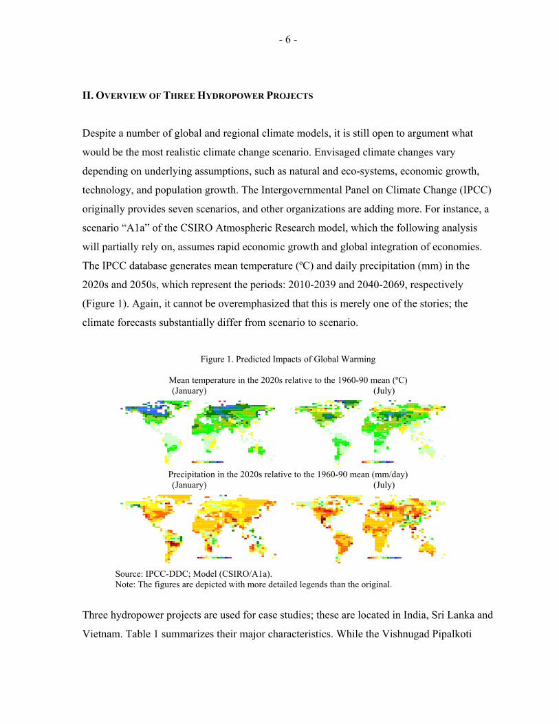
II. OVERVIEW OF THREE HYDROPOWER PROJECTS

Despite a number of global and regional climate models, it is still open to argument what

would be the most realistic climate change scenario. Envisaged climate changes vary

depending on underlying assumptions, such as natural and eco-systems, economic growth,

technology, and population growth. The Intergovernmental Panel on Climate Change (IPCC)

originally provides seven scenarios, and other organizations are adding more. For instance, a

scenario “A1a” of the CSIRO Atmospheric Research model, which the following analysis

will partially rely on, assumes rapid economic growth and global integration of economies.

The IPCC database generates mean temperature (ºC) and daily precipitation (mm) in the

2020s and 2050s, which represent the periods: 2010-2039 and 2040-2069, respectively

(Figure 1). Again, it cannot be overemphasized that this is merely one of the stories; the

climate forecasts substantially differ from scenario to scenario.

Figure 1. Predicted Impacts of Global Warming

Mean temperature in the 2020s relative to the 1960-90 mean (ºC)

(January) (July) 4 3 2 1 1 1 1 1 1 1 1 1 1 2 13 17 3

4 4 4 3 1 2 1 1 2 1 1 1 1 1 13 3 8 2 2 1 1 1 0 6 2 2 2 2 2

3 2 3 4 5 4 2 2 1 1 4 1 2 4 4 4 3 3 2 2 2 2 2 3 2 2 2 2 2 2 23 3 2 2 3 3 3 3 3 3 3 4 5 2 2 2 2 0 1 2 2 2 3 3 2 3 3 3 3 3 3 3 3 3 2 2 2 2 2 2 1 2 2 1 0 0 1

6 3 4 3 2 2 3 3 3 3 3 3 3 3 6 11 1 1 1 2 0 1 0 1 2 3 3 3 3 3 3 3 3 3 3 3 3 2 2 2 2 1 1 1 2 2 2 1 1 1 22 3 2 2 2 4 3 3 3 4 3 3 2 0 1 1 1 2 2 2 3 3 3 2 2 2 2 2 2 2 2 2 2 2 1 1 1 2 2 3 6 1 2

2 2 3 3 3 4 4 3 3 4 2 2 1 2 2 2 3 3 3 2 2 2 2 2 2 2 2 2 2 2 2 2 2 2 21 2 2 3 3 3 3 3 3 4 4 2 2 1 2 2 2 2 3 3 3 2 2 2 2 2 1 1 2 2 2 2 2 2 3 2

2 2 2 2 3 3 3 3 3 3 2 2 1 1 2 2 2 2 2 2 2 3 3 3 2 2 2 2 1 1 1 2 2 2 2 2 3 9 11 2 2 2 2 2 2 2 2 2 2 1 2 2 1 2 2 2 1 2 2 2 3 3 2 3 2 2 2 1 1 1 1 2 2 1 2

2 1 2 2 2 2 2 2 2 2 2 2 1 1 1 2 1 1 1 1 2 3 3 1 2 2 3 2 1 1 1 1 1 1 11 2 1 1 1 2 2 1 1 1 2 1 1 1 1 2 2 3 0 2 2 1 1 1 1 1 1 1 1 1

1 2 1 1 1 2 1 1 1 1 1 1 1 1 1 1 2 2 2 0 0 1 1 1 2 2 2 1 11 1 1 1 1 1 1 0 2 2 1 1 2 1 1 2 2 2 2 0 1 2 1 2 2 2 2 0 0

1 1 0 1 1 1 2 2 2 1 1 2 2 2 2 2 2 2 2 0 2 2 2 2 2 21 1 1 1 2 2 2 2 1 1 1 1 2 2 1 1 2 2 2 1 1 1 1 1 1 2 11 1 2 2 2 2 1 1 1 1 1 2 2 1 1 1 2 1 1 1 1 1 1 1 0

1 2 2 2 2 1 1 1 1 1 2 2 2 1 2 2 1 0 1 1 1 01 1 2 2 2 2 2 2 1 1 1 1 1 1 1 1 0 1 1

1 1 2 1 1 1 1 1 1 1 1 1 1 1 1 1 0 1 01 1 1 1 1 1 1 1 1 1 1 1 1 0 1 01 1 1 1 1 1 1 1 1 1 1 1 1 1 1 1 1 0 1

1 1 1 1 1 1 1 1 1 1 1 1 1 0 01 1 1 1 1 1 1 0 0 1 1 1 1

1 1 1 1 1 1 1 0 0 1 1 0 1 1 10 1 1 1 1 1 1 1 1 1 1 1 1 0 1 1 1 11 1 1 1 1 1 1 0 1 1 1 0 0 1 1 1

1 1 1 1 1 1 0 1 1 1 0 0 11 1 1 1 1 1 0 1 1 1 0 1 01 1 1 1 1 1 1 1 1 0 0 1 1 0

1 1 2 1 1 1 1 0 0 0 1 1 0 1 11 1 1 1 1 1 1 1 1 1 2 1 0 0 1 21 1 1 1 1 1 1 1 1 1 0 1 2 11 1 1 1 1 1 1 1 1 1 1 1 1 11 1 1 1 1 1 0 1 1 1 11 1 1 1

0 1 0 0 10 1 10 1 10 0 -2 -1 -.5 0- 0.5- 1- 1.5- 2- 2.5- 3- 4- 5- 6-0

0

0 1 1 5 6 6 3 2 2 2 2 2 2 1 3 2 -00 0 0 0 1 1 4 2 3 2 2 2 2 0 1

3 1 2 2 2 2 2 2 1 2 2 2 2 2 21 1 1 2 1 2 4 1 2 1 2 1 1 1 1 1 1 1 1 2 2 1 1 1 1 1 1 0 1 0 0

1 1 1 1 3 1 2 1 1 1 1 1 0 1 2 1 1 -1 0 1 1 1 1 1 1 1 1 1 1 1 1 1 2 2 1 1 1 1 1 1 1 1 1 0 0 1 21 -1 -0 1 -0 -0 -0 1 -0 -0 -0 -0 -1 -1 1 1 1 1 1 3 0 1 -1 -0 0 0 -0 -0 -0 0 0 0 0 1 1 0 0 0 -0 -0 -0 -1 -1 -1 -1 -0 -1 -1 -0 0 0

2 -1 1 1 1 -1 -1 -1 -1 -0 0 -1 -1 0 1 -1 -1 2 0 0 0 0 -0 -0 -0 0 1 1 1 1 0 0 -0 -1 -0 -1 -1 -1 -1 -1 1 0 21 1 0 0 -0 0 0 1 0 0 0 1 1 0 1 1 1 1 1 1 0 1 1 2 2 1 1 1 1 1 0 0 0 0 0

1 1 1 1 2 2 2 2 2 2 1 1 2 1 2 2 2 3 3 3 3 2 2 0 3 3 2 2 2 2 2 2 2 1 2 22 2 2 2 2 2 2 2 2 2 2 2 1 1 1 1 2 2 2 2 3 3 3 2 2 2 3 3 2 2 2 2 2 2 2 1 2 -0 22 2 2 2 2 3 3 3 2 2 2 2 1 1 1 1 2 2 1 2 2 2 3 2 2 2 3 2 2 2 2 2 2 2 2 1 1

2 2 2 2 2 3 3 2 2 2 2 1 1 1 1 2 1 1 1 3 2 2 2 3 2 2 2 2 1 2 1 1 1 1 12 2 2 2 2 2 2 2 2 2 2 1 2 2 3 2 2 2 2 1 2 2 1 1 1 1 1 1 1 1

2 2 2 2 2 2 1 1 1 1 1 1 1 2 2 2 2 2 2 2 1 1 2 2 1 1 1 1 11 2 2 1 1 1 1 1 1 2 2 1 2 2 2 2 2 2 2 1 1 3 1 1 1 0 1 1 1

1 2 1 0 0 1 2 2 2 1 1 2 1 2 2 2 2 1 2 2 1 1 1 0 0 12 1 1 1 2 2 2 1 1 1 2 2 2 2 1 1 2 1 1 1 1 1 1 1 0 0 12 1 1 2 1 1 1 1 2 2 2 2 1 2 1 1 1 0 0 0 1 1 1 1 1

1 2 2 2 1 1 1 2 2 2 2 2 2 2 0 -0 0 0 1 1 1 11 1 1 2 1 1 1 2 2 2 1 2 2 1 -0 0 0 1 1

1 1 1 1 1 1 1 1 2 2 2 2 1 1 0 0 1 1 11 1 1 1 1 1 1 1 1 1 1 1 1 1 1 01 1 1 1 1 1 1 1 1 1 1 1 1 1 1 1 1 0 1

1 1 1 1 1 1 1 1 1 1 1 1 1 0 11 1 1 1 1 1 1 1 1 1 1 1 1

1 1 1 1 1 1 1 1 1 1 1 1 1 0 11 1 1 1 1 1 1 1 1 1 1 1 1 1 0 0 1 11 1 1 1 1 1 1 1 1 1 1 1 1 1 1 1

1 1 1 1 1 1 1 1 1 1 1 1 01 1 1 1 1 1 1 1 1 1 1 1 11 1 1 1 1 1 0 1 1 1 1 1 0 0

1 1 1 1 1 1 1 1 1 1 1 0 0 1 11 1 1 1 1 1 1 1 1 1 1 1 1 1 1 12 1 1 1 1 1 1 1 1 1 1 1 1 11 1 1 1 1 1 1 1 1 1 1 1 1 11 1 0 1 1 1 0 1 1 1 11 1 0 0

1 1 1 0 11 1 11 1 11 1 -2 -1 -.5 0- 0.5- 1- 1.5- 2- 2.5- 3- 4- 5- 6-1

0 Precipitation in the 2020s relative to the 1960-90 mean (mm/day)

(January) (July) -0 -0 -0 -0 -0 -0 -0 -0 -0 -0 -0 -0 -0 -0 1 1 -0

-0 0 0 -0 -0 -0 -0 -0 -0 -0 -0 -0 -0 -0 -0-0 0 -0 -0 -0 -0 -0 -0 -0 0 -0 -0 -0 -0 -0

0 -0 0 0 0 0 -0 -0 -0 -0 0 -0 0 0 0 0 0 0 -0 -0 -0 -0 -0 -0 -0 -0 -0 -0 -0 -0 -00 0 0 0 0 0 0 0 0 0 -0 -0 0 -0 -0 0 0 -0 -0 0 0 0 0 0 0 0 0 0 0 0 0 0 0 -0 -0 -0 -0 -0 -0 -0 -0 -0 -0 -0 -0 -0 -0

1 0 0 0 0 0 0 0 0 0 0 0 0 0 0 1 -1 -1 -0 0 -0 -0 0 0 0 0 0 0 0 0 0 0 -0 0 0 0 0 0 -0 -0 -0 -0 -0 -0 -0 -0 -0 -0 -0 -0 -00 0 1 1 1 1 0 0 -0 0 0 0 -0 0 -0 0 0 0 0 0 0 0 0 -0 -0 -0 -0 -0 -0 0 0 0 -0 -0 -0 -0 -0 -0 -0 -0 0 -0 0

1 1 1 0 -0 0 0 0 0 -0 -0 -0 0 0 0 0 0 0 0 0 0 0 0 -0 -0 -0 0 0 0 -0 -0 -0 -0 -0 -00 -0 0 -0 -0 0 0 0 0 0 -0 -0 0 -0 0 0 0 0 0 0 0 0 0 0 -0 0 0 0 -0 -0 -0 -0 -0 -0 0 -0

-0 0 -0 -0 -0 -0 -0 -0 -0 -0 -0 -0 0 -0 -0 0 0 0 0 0 0 -0 0 0 -0 -0 0 0 0 0 -0 -0 -0 -0 -0 0 0 1 -0-0 0 0 -0 -0 -0 -0 -0 -0 -0 -0 -0 0 0 0 0 0 0 -0 -0 -0 -0 -0 -0 -0 -0 0 -0 -0 0 -0 -0 -0 -0 -0 0 0

-0 -0 -0 -0 -0 -0 -0 -0 -0 -0 -0 0 0 0 0 0 -0 -0 -0 -0 -0 -0 -0 -0 -0 -0 -0 0 -0 -0 -0 -0 -0 -0 -0-0 -1 -0 -0 0 -0 -0 -0 -0 -0 0 0 -0 -0 -0 -0 -0 -0 -0 -0 -0 -0 -0 -0 -0 -0 -0 -0 -0 -0

-1 -0 -0 -0 -0 -0 -0 -0 0 -0 -0 -0 -0 -0 -0 -0 -0 -0 -0 -0 -0 -0 -0 -0 -0 -0 -0 -0 -0-0 -0 -0 -0 -0 -0 -0 -0 -0 -0 -0 -0 -0 -0 -0 -0 -0 -0 -0 -0 -0 -0 -0 -0 -0 -0 -0 -1 -1

-0 -0 -0 -0 0 -0 -0 -0 -0 -0 -0 -0 -0 0 0 -0 -0 -0 -1 -1 -0 0 0 -0 -0 -0-0 -0 0 0 -0 -0 -0 -0 -0 -0 -0 -0 -0 0 0 -0 -0 -0 -0 -0 -0 -0 0 -0 -0 -0 -00 0 -0 -0 -0 -0 -0 -0 -0 -0 -0 -0 -0 -0 -0 -0 -0 0 0 0 0 0 0 0 -0

1 -0 -0 -0 -0 -0 -0 -0 -0 -0 -0 -0 -0 -0 0 0 -0 -0 0 -0 0 -01 0 -0 -0 -0 -0 -0 -0 -0 -0 -0 -0 -0 -0 0 -0 -1 -0 -0

-0 -0 -0 -0 -0 -0 -0 -0 -0 -0 -0 -0 -0 -0 0 -0 -0 -0 -0-0 -0 -0 -0 -0 -0 -0 -0 -0 -0 -0 -0 0 -0 0 1-0 0 -0 -0 -0 -0 -0 0 0 -0 -0 -0 -0 -0 -0 -0 1 1 1

0 -0 -0 -0 -0 0 0 0 0 0 0 0 -0 0 10 0 0 -0 -0 -0 0 0 -0 0 0 -0 0

0 0 -0 -0 0 0 0 0 -0 -1 0 0 0 -0 10 -0 0 0 0 0 0 1 -0 0 0 -0 0 0 -0 -0 2 10 -0 0 1 1 0 1 1 -0 1 0 1 0 -1 1 0

0 -0 0 0 0 0 1 -1 0 0 1 1 0-0 -1 -1 -0 0 0 1 0 0 0 1 0 2-0 -0 -1 -1 -1 -1 0 0 -0 0 1 0 0 1

-0 -1 -1 -1 -1 0 -1 0 0 0 -1 -0 1 1 0-0 -0 -0 -0 -0 -0 -0 -0 0 -0 -0 -0 0 1 0 0-0 0 0 0 -0 -1 -1 -0 -1 0 0 0 -0 -0-0 0 0 0 -0 -0 -1 -0 -0 -0 0 0 0 0-0 -0 -0 -0 -0 -0 -0 0 -0 0 0-0 -0 -0 -0

-0 -0 -0 -0 -00 -0 -.75 -.5 -0.2 0- .25- .5- .75- 1- 1.5- 2- 3- 4- 5- -00 -0 0

-0 -0-0

-0

-0 -0 -0 -0 -0 -0 0 0 0 0 0 0 0 0 0 0 00 0 -0 -0 -0 -0 -0 -0 -0 -0 -0 -0 0 -0 -0

0 -0 -0 -0 -0 -0 -0 -0 -0 0 0 -0 -0 -0 -00 0 0 0 -0 -0 -0 0 0 -0 -0 -0 -0 -0 0 0 1 0 0 0 -0 -0 -0 0 0 0 0 -0 0 0 0

0 0 0 0 0 0 0 -0 -0 1 0 -0 -0 -0 -0 0 0 -0 0 0 -0 0 0 0 -0 0 0 0 0 0 0 0 0 0 -0 -0 -0 0 0 0 0 1 1 0 0 0 0-0 0 0 0 0 0 0 0 0 0 1 0 0 -0 -0 -0 -0 -0 0 0 -0 -0 0 1 -0 -0 0 0 -0 0 0 0 -0 0 0 0 0 0 0 -0 -0 -0 0 0 0 1 1 0 0 0 0

-0 -0 -0 -0 0 0 0 0 0 1 0 0 0 1 -0 -0 0 0 -0 -0 -0 -0 -0 -0 0 0 0 0 -0 -0 -0 -0 -0 -0 -0 -0 -0 0 0 0 0 0 0-0 0 0 0 -0 -0 -0 0 0 0 0 1 0 0 -0 -1 -1 -1 -1 -1 -0 -0 -0 -0 -0 -0 -0 -0 -0 0 0 -0 0 0 -0

0 -0 -0 -0 -1 -0 -0 0 -0 -0 -0 0 0 0 -0 -1 -1 -1 -1 -1 -1 -0 -0 -0 -0 -0 0 0 -0 -0 -0 -0 -0 0 0 0-0 -0 -0 -0 -1 -1 -1 -0 -0 -0 -0 -0 -0 -0 0 0 0 -0 -0 -0 -0 -0 -0 -0 -0 -0 -0 -0 0 -0 -0 -0 -0 -0 -0 0 0 -0 -0-0 -0 -0 -0 -1 -1 -1 -1 -0 -0 0 0 -0 -0 -0 0 -0 -0 -0 -0 -0 -0 -0 -0 -0 -0 -0 0 -0 -1 -0 -0 -0 -0 -0 1 0

-0 -0 -0 -0 -0 -0 -0 -0 -0 0 0 -0 -0 -0 -0 -1 -0 -0 -0 -0 -0 -0 -0 -0 1 0 -0 -0 -0 -0 -0 -1 -0 0 0-0 -0 -0 -0 -0 -0 -0 -0 -0 -0 -0 -0 -0 -0 -1 -0 -0 -0 -0 -0 -0 -0 0 0 -0 -1 -0 -0 -0 0

-0 -0 -1 -0 -0 -0 0 0 -0 -0 -0 -0 -0 -0 -0 -0 -0 -0 -0 0 -0 0 1 0 -0 -1 -1 1 -0-0 -0 -1 1 0 0 0 0 -0 -0 -0 -0 -0 -0 -0 -0 -0 -0 -0 -0 0 1 0 -0 -1 0 0 1 -0

-0 -1 1 0 0 0 -0 -0 -0 -0 -0 -0 -0 -0 -0 -0 -0 -0 -0 -0 1 0 0 0 0 1-1 0 0 0 -0 -0 -0 -0 -0 -0 -0 -0 -0 -0 -0 -0 -0 -0 -0 0 0 0 0 1 1 0 1-1 -0 -0 -0 -0 -0 -0 -0 -0 -0 -0 -0 -0 -0 -0 -0 -0 0 1 1 1 0 1 1 0

-0 -0 -0 -0 -0 -0 -0 -0 -0 -0 -0 -0 -0 -0 0 -0 0 0 -0 -0 -0 1-0 -0 -0 -0 -0 -0 -0 -0 -0 -0 -0 -0 -0 -0 1 1 1 -0 -0

-1 -1 -0 -1 -0 -0 -0 0 -0 -0 -0 -0 -0 -0 0 0 -0 -0 -1-0 -0 -0 -0 -0 -0 -0 -0 -0 -0 -0 -0 -1 -1 -1 10 0 0 0 0 -0 -0 0 -0 -0 -0 -0 -0 -0 -0 -0 0 -0 0

0 0 0 -0 0 0 -0 -0 0 0 -0 -0 -0 -1 -0-0 -0 -0 0 0 -0 -0 -0 0 0 -0 -0 0

0 -0 -0 -0 -0 -0 -0 -0 0 0 -0 -0 -0 -0 0-0 -0 -0 -0 -0 -0 -0 -0 -0 -0 -0 -0 -0 -0 -0 -0 -0 0-0 -0 -0 -0 -0 -0 -0 -0 -0 -0 -0 -0 -0 -0 0 0

-0 -0 -0 -0 -0 -0 0 -0 -0 -0 -0 0 -1-0 -0 -0 -0 -0 -0 -0 -0 -0 -0 -0 0 -0-0 -0 -0 -0 -0 -0 -1 -0 -0 -0 -0 0 -0 -0

-0 -0 -0 -0 -0 -0 -0 -0 -0 -0 -0 -0 -0 -0 0-0 -0 -0 -0 -0 -0 -0 -0 -0 -0 0 -0 -0 -0 0 -0-0 -0 -0 -0 -0 -0 -0 0 0 -0 -0 -0 -0 -0-0 -0 -0 -0 -0 -0 -0 -0 -0 -0 -0 -0 -0 0-0 -0 -0 -0 -0 -0 -0 -0 -0 -0 -0-0 -0 -0 -0

0 0 -0 -0 00 0 -.75 -.5 -0.2 0- .25- .5- .75- 1- 1.5- 2- 3- 4- 5- -01 0 00 0

-0-0

Source: IPCC-DDC; Model (CSIRO/A1a). Note: The figures are depicted with more detailed legends than the original.

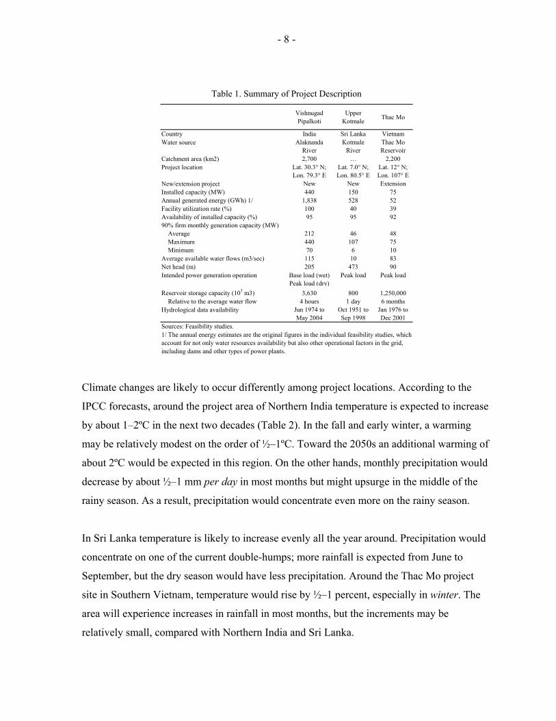
Three hydropower projects are used for case studies; these are located in India, Sri Lanka and

Vietnam. Table 1 summarizes their major characteristics. While the Vishnugad Pipalkoti

- 7 -

Hydro Electric Project (VPHEP) in India is still in preparation, the other two, the Upper

Kotmale Hydro Power Project (UKHPP) in Sri Lanka and the Thac Mo Hydropower Station

Extension Project (TMHSEP) in Vietnam, have already been launched.

The selected projects look very different in various aspects. The Vishnugad Pipalkoti project

will be a typical “run-of-river” station though it has a small storage capacity for diurnal

variations. On the other hand, the Upper Kotmale project includes a daily reservoir of

800,000 m3, which allows it to operate for peak load power generation. Correspondingly, its

plant utilization rate is assumed 40 percent. The Thac Mo project aims to extend the existing

generation capacity of 150 MW and relies for water resources on the existing large Thac Mo

Reservoir, which lies about 100 km north of Ho Chi Minh City.

How to operate a hydropower plant is largely dependent on the reservoir capacity. VPHEP is

expected to contribute to providing base load energy during the rainy season, which is

consistent with the basic fact that Northern India still lacks electricity in absolute terms,

possibly owing to the recent economic buoyancy. In the dry season it may supply peak load

energy using its attached hourly storage. The other two projects basically aim to operate on a

peak load basis. In Sri Lanka, the Upper Kotmale project is one of the last large-scale

hydropower projects. Most water resources have already been utilized in this country. The

extended part of the Thac Mo hydropower station will provide energy to meet the residual

demand that the existing plant cannot supply.

The three projects also differ in size and cost. While the VPHEP is intended to generate

about 1,800 GWh of energy per annum, the much smaller amount of energy will be delivered

by the UKHPP and TMHSEP. The Upper Kotmale project may cost about 300 million U.S.

dollars, but the total cost of the Thac Mo project was estimated at 50 million U.S. dollars

because it is a relatively small extension work and does not include any new storage

construction.

- 8 -

Table 1. Summary of Project Description

Vishnugad Pipalkoti

Upper Kotmale Thac Mo

Country India Sri Lanka VietnamWater source Alaknanda

RiverKotmale

RiverThac Mo Reservoir

Catchment area (km2) 2,700 … 2,200Project location Lat. 30.3° N;

Lon. 79.3° ELat. 7.0° N; Lon. 80.5° E

Lat. 12° N; Lon. 107° E

New/extension project New New ExtensionInstalled capacity (MW) 440 150 75Annual generated energy (GWh) 1/ 1,838 528 52Facility utilization rate (%) 100 40 39Availability of installed capacity (%) 95 95 9290% firm monthly generation capacity (MW) Average 212 46 48 Maximum 440 107 75 Minimum 70 6 10Average available water flows (m3/sec) 115 10 83Net head (m) 205 473 90Intended power generation operation Base load (wet)

Peak load (dry)Peak load Peak load

Reservoir storage capacity (103 m3) 3,630 800 1,250,000 Relative to the average water flow 4 hours 1 day 6 monthsHydrological data availability Jun 1974 to

May 2004Oct 1951 to Sep 1998

Jan 1976 to Dec 2001

Sources: Feasibility studies. 1/ The annual energy estimates are the original figures in the individual feasibility studies, which account for not only water resources availability but also other operational factors in the grid, including dams and other types of power plants.

Climate changes are likely to occur differently among project locations. According to the

IPCC forecasts, around the project area of Northern India temperature is expected to increase

by about 1–2ºC in the next two decades (Table 2). In the fall and early winter, a warming

may be relatively modest on the order of ½–1ºC. Toward the 2050s an additional warming of

about 2ºC would be expected in this region. On the other hands, monthly precipitation would

decrease by about ½–1 mm per day in most months but might upsurge in the middle of the

rainy season. As a result, precipitation would concentrate even more on the rainy season.

In Sri Lanka temperature is likely to increase evenly all the year around. Precipitation would

concentrate on one of the current double-humps; more rainfall is expected from June to

September, but the dry season would have less precipitation. Around the Thac Mo project

site in Southern Vietnam, temperature would rise by ½–1 percent, especially in winter. The

area will experience increases in rainfall in most months, but the increments may be

relatively small, compared with Northern India and Sri Lanka.

- 9 -

Table 2. IPCC Climate Projections around Project Sites

Avg. Proj. Avg. Proj. Avg. Proj. Avg. Proj. Avg. Proj. Avg. Proj.1961-90 2020s 1961-90 2020s 1961-90 2020s 1961-90 2020s 1961-90 2020s 1961-90 2020s

Jan 6.3 7.3 47 34 26.6 27.3 63 97 21.5 21.9 44 51Feb 7.2 8.0 55 47 26.9 27.6 71 68 22.5 22.7 26 38Mar 11.0 12.2 58 39 27.7 28.3 129 137 20.0 20.8 34 73Apr 15.5 17.2 35 6 28.2 28.8 255 252 25.5 26.1 48 61May 17.8 19.7 66 52 28.3 28.9 401 335 26.2 26.3 122 135Jun 18.6 20.0 138 135 27.9 28.7 179 187 26.5 26.4 154 167Jul 17.4 18.2 327 340 27.6 28.4 130 138 26.6 27.0 170 135Aug 17.0 17.4 293 332 27.5 28.3 92 111 26.8 27.2 160 168Sep 16.2 16.3 201 198 27.5 28.3 241 289 25.7 26.3 311 313Oct 14.3 15.1 43 56 27.0 27.6 382 379 25.1 25.7 363 397Nov 11.1 11.5 7 0 26.7 27.4 308 285 23.7 24.3 312 309Dec 8.4 9.6 24 27 26.6 27.2 170 156 22.2 23.1 110 113

Precipitation (mm/month)

Sources: IPCC DDC database and one of the SRES scenarios, CSIRO/A1a; and NOAA GHCN Monthly database version 2. Note that the estimated incremental changes are given by the IPCC model. The historical series are based on NOAA database for VPHEP and UKHPP. The Thac Mo case relies on IPCC DDC database for historical data as well.

Vishinugad Pipalkoti (India) Upper Kotmale (Sri Lanka) Thac Mo (Vietnam)

Temperature (°C)Precipitation (mm/month) Temperature (°C)

Precipitation (mm/month)Temperature (°C)

III. MODEL AND DATA

Following the existing literature (e.g., Salas, 1993; Mohammadi et al., 2006), a simple

multivariate stochastic model, VAR, is considered. Stationarity is a key requirement for

performing the VAR model. Hydrologic data defined on an annual time scale are generally

characterized stationary unless there are large-scale climate variability, natural disruptions

and human-induced changes such as reservoir construction (Salas, 1993). A typical

hydrologic process is composed of three parts: (i) a deterministic part resulting from natural

physical periodicities, (ii) an aperiodic deterministic part which is often referred to as trends,

and (iii) a stationary random component. Once detrending and adjusting seasonarity, the

remaining time series tends to be covariance stationary (Koutsoyiannis, 2006).

Our hydrological data seem to have strong seasonal regularities on an annual basis

(Figure 2). Outstanding hikes in water flow have been observed twice a year in the Sri

Lanka’s case and once a year in the rest of the cases. Another intuitive finding from the

figure is that while a water flow in the Kotmale River appears to have declined over the past

five decades, the Thac Mo discharge may have had an increasing steady tendency in recent

- 10 -

years. The feasibility sturdy recognizes the fact that the discharge at the Thac Mo Reservoir

has increased since the construction of the original dam. The Alaknanda River does not seem

to have a significant time trend component.

Figure 2. Observed Monthly Hydrology

(Vishnugad Pipalkoti, India) (Upper Kotmale, Sri Lanka)

010

0020

0030

00

Hyd

rolo

gy(m

il. m

3 pe

r mon

th)

1970m1 1975m1 1980m1 1985m1 1990m1 1995m1 2000m1 2005m1Year and month

050

100

150

200

Hyd

rolo

gy(m

il. m

3 pe

r mon

th)

1950m1 1960m1 1970m1 1980m1 1990m1 2000m1Year and month

(Thac Mo, Vietnam)

050

010

0015

00

Hyd

rolo

gy(m

il. m

3 pe

r mon

th)

1975m1 1980m1 1985m1 1990m1 1995m1 2000m1Year and month

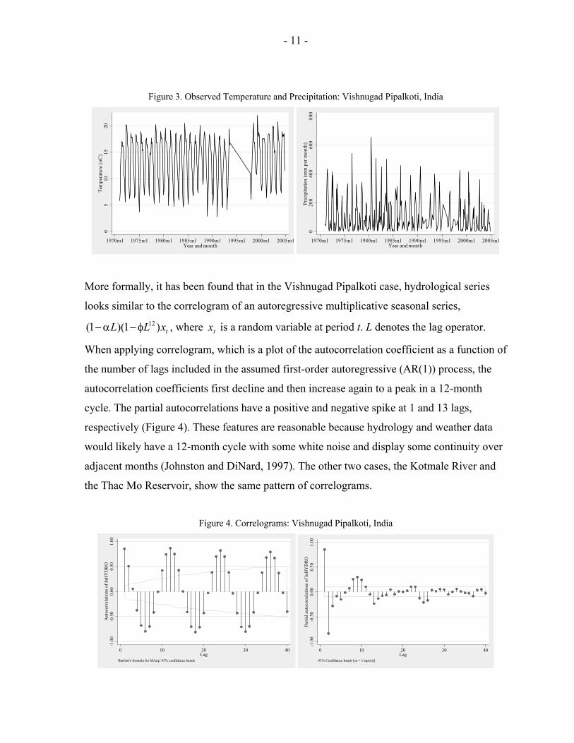
In addition to hydrology, both precipitation and temperature series are also apt to exhibit

considerable seasonality. However, it is common that the former has more irregularities than

the latter (Figure 3).2

2 In these time series borrowed from the NOAA database, some observations are missing in the 1990s.

- 11 -

Figure 3. Observed Temperature and Precipitation: Vishnugad Pipalkoti, India 0

510

1520

Tem

pera

ture

(oC

)


020

040

060

080

0Pr

ecip

itatio

n (m

m p

er m

onth

)


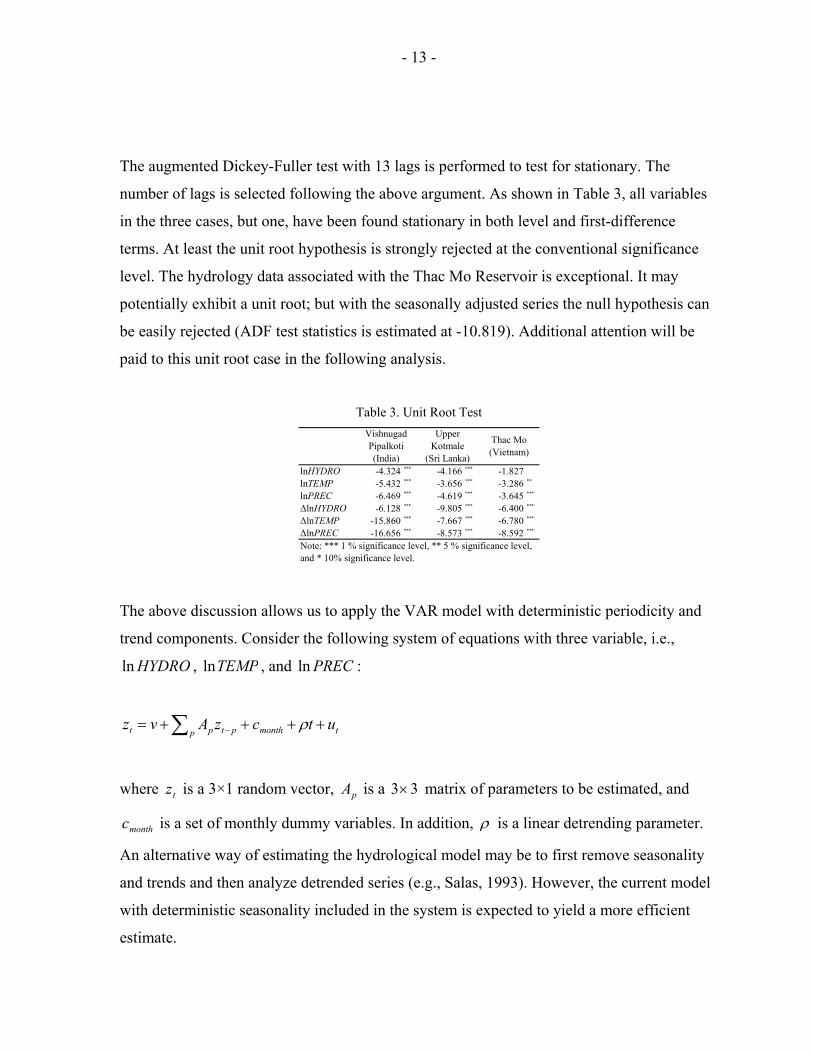
More formally, it has been found that in the Vishnugad Pipalkoti case, hydrological series

looks similar to the correlogram of an autoregressive multiplicative seasonal series,

txLL )1)(1( 12φ−α− , where tx is a random variable at period t. L denotes the lag operator.

When applying correlogram, which is a plot of the autocorrelation coefficient as a function of

the number of lags included in the assumed first-order autoregressive (AR(1)) process, the

autocorrelation coefficients first decline and then increase again to a peak in a 12-month

cycle. The partial autocorrelations have a positive and negative spike at 1 and 13 lags,

respectively (Figure 4). These features are reasonable because hydrology and weather data

would likely have a 12-month cycle with some white noise and display some continuity over

adjacent months (Johnston and DiNard, 1997). The other two cases, the Kotmale River and

the Thac Mo Reservoir, show the same pattern of correlograms.

Figure 4. Correlograms: Vishnugad Pipalkoti, India

-1.0

0-0

.50

0.00

0.50

1.00

Aut

ocor

rela

tions

of l

nHY

DR

O

0 10 20 30 40Lag

Bartlett's formula for MA(q) 95% confidence bands

-1.0

0-0

.50

0.00

0.50

1.00

Parti

al a

utoc

orre

latio

ns o

f lnH

YD

RO

0 10 20 30 40Lag

95% Confidence bands [se = 1/sqrt(n)]

- 12 -

When removing monthly periodicities in a deterministic manner, hydrologic and weather

series indeed come to exhibit clearer stationarity. Figure 5 depicts the seasonally adjusted

time series of the Vishnugad Pipalkoti case, for example. Some extreme observations—

compared with the long-term monthly mean—remain striking; however, the seasonality

disappears. Of particular note, in this case the seasonally adjusted precipitation series may

have a declining time trend especially in the past ten years, while no clear trend can be

detected graphically in hydrology and temperature series.3

Figure 5. Seasonally Adjusted Time Series: Vishnugad Pipalkoti, India

(Hydrology) (Temperature)

-100

00

1000

2000

Seas

onal

ly a

djus

ted

hydr

olog

y(m

il. m

3 pe

r mon

th)


05

1015

Seas

onal

ly a

djus

ted

tem

pera

ture

(oC

)


(Precipitation)

-200

020

040

0Se

ason

ally

adj

uste

d pr

ecip

itatio

n (m

m p

er m

onth

)


3 There might be a much longer term trend in climate time series, which is not taken into account in the current analysis. Goswami et al. (2006) show that India’s precipitation time series exhibits a long-term trend over the last 50 years.

- 13 -

The augmented Dickey-Fuller test with 13 lags is performed to test for stationary. The

number of lags is selected following the above argument. As shown in Table 3, all variables

in the three cases, but one, have been found stationary in both level and first-difference

terms. At least the unit root hypothesis is strongly rejected at the conventional significance

level. The hydrology data associated with the Thac Mo Reservoir is exceptional. It may

potentially exhibit a unit root; but with the seasonally adjusted series the null hypothesis can

be easily rejected (ADF test statistics is estimated at -10.819). Additional attention will be

paid to this unit root case in the following analysis.

Table 3. Unit Root Test

lnHYDRO -4.324 *** -4.166 *** -1.827lnTEMP -5.432 *** -3.656 *** -3.286 **

lnPREC -6.469 *** -4.619 *** -3.645 ***

ΔlnHYDRO -6.128 *** -9.805 *** -6.400 ***

ΔlnTEMP -15.860 *** -7.667 *** -6.780 ***

ΔlnPREC -16.656 *** -8.573 *** -8.592 ***

Vishnugad Pipalkoti (India)

Upper Kotmale

(Sri Lanka)

Thac Mo (Vietnam)

Note: *** 1 % significance level, ** 5 % significance level, and * 10% significance level.

The above discussion allows us to apply the VAR model with deterministic periodicity and

trend components. Consider the following system of equations with three variable, i.e.,

HYDROln , TEMPln , and PRECln :

∑ ++++= −p tmonthptpt utczAvz ρ

where tz is a 3×1 random vector, pA is a 33× matrix of parameters to be estimated, and

monthc is a set of monthly dummy variables. In addition, ρ is a linear detrending parameter.

An alternative way of estimating the hydrological model may be to first remove seasonality

and trends and then analyze detrended series (e.g., Salas, 1993). However, the current model

with deterministic seasonality included in the system is expected to yield a more efficient

estimate.

- 14 -

HYDRO is defined as the monthly discharge (in million cubic meters (m3)) of each river at

the project site. The data come from each of feasibility studies. Temperature and

precipitation data depend on the NOAA GHCN Monthly Database Version 2; the data from

the observatory closest to the project location are used.4 In the NOAA database, however,

there is no available comprehensive data for Southern Vietnam. Alternatively, the observed

regional weather time series provided by the IPCC Data Distribution Centre (DDC) are

borrowed.5 But unlike the NOAA database, these time series are available only up to 1990,

and may have poor spatial representation. Thus, when using them, we may risk

underestimating the most recent impacts of global warming. Whereas TEMP is defined as the

monthly average temperature converted to Fahrenheit in order to avoid taking logarithms of

negative numbers, PREC is total monthly rainfall measured in millimeters (mm).6 When

there is no precipitation in a particular month, it is set to a very small positive number, but

not zero.

How are these three variables related to each other? Table 4 shows simple correlations. The

extent to which hydrology is linked to climate differs among project locations. Precipitation

may be most relevant to hydrological series. However, temperature may be positively or

negatively associated with river flow. There is no serious multicollineality problem in our

data.

Table 4. Simple Correlation


Upper Kotmale

(Sri Lanka)

Thac Mo (Vietnam)

(lnHYDRO , lnTEMP ) 0.774 -0.360 0.465(lnHYDRO , lnPREC ) 0.271 0.285 0.849(lnTEMP , lnPREC ) 0.117 0.030 0.551No of obs. 295 496 240

4 The Mukteshwar observatory (lat. 29.5° north; long. 79.7° east) provides data to the Vishnugad Pipalkoti case; and data from Colombo (lat. 6.9° north; long. 79.9° east) are borrowed. 5 The latitude and longitude of the specified point are 12° north and 107° east, respectively. 6 The NOAA database provides precipitation time series per day, which is thus converted to monthly series in the Thac Mo case.

- 15 -

An important specification question in using the VAR-type model is how many lags should

be included in the system. When removing periodicities on a unilateral variable basis, the

correlograms of seasonally adjusted hydrologic series may suggest that in the Vishnugad

Pipalkoti case, for instance, the first three or four orders might be autocorrelated (Figure 6).

Formally, the Akaike’s information criterion (AIC) lag-order selection statistics is estimated

(Akaike, 1973). As shown in Table 5, the maximum number of lags to be included in the

model is 2 and 3 for the Vishnugad Pipalkoti and Upper Kotmale cases, respectively. In the

Thac Mo hydro case, only one lag may need including. These results are robust, regardless of

whether or not a time trend component is introduced in the model.

Figure 6. Correlograms of Seasonally Adjusted Hydrology: Vishnugad Pipalkoti, India

-0.2

00.

000.

200.

400.

600.

80

Aut

ocor

rela

tions

of s

easo

nally

adj

uste

d hy

drol

ogy

(mil.

m3

per m

onth

)

0 10 20 30 40Lag

Bartlett's formula for MA(q) 95% confidence bands

Table 5. Lag Selection Criteria

LagLog

likelihoodAIC

statisticsLog

likelihoodAIC

statisticsLog

likelihoodAIC

statisticsLog

likelihoodAIC

statisticsLog

likelihoodAIC

statisticsLog

likelihoodAIC

statistics0 -349.9 3.820 -339.0 3.743 110.1 -0.370 184.0 -0.723 673.8 -5.405 696.3 -5.5701 -215.8 2.582 -209.1 2.545 256.8 -1.056 279.7 -1.155 737.8 -5.871 ** 747.0 -5.924 **

2 -203.2 2.546 ** -197.5 2.520 ** 286.9 -1.162 299.4 -1.209 741.7 -5.828 749.5 -5.8693 -197.5 2.579 -192.3 2.558 303.5 -1.199 ** 311.2 -1.223 ** 751.2 -5.832 756.6 -5.8524 -191.3 2.607 -185.9 2.583 307.1 -1.172 315.0 -1.197 756.3 -5.799 761.0 -5.814

Note: *** 1 % significance level, ** 5 % significance level, and * 10% significance level.

Thac Mo (Vietnam)W/o trend With trendW/o trend

Vishnugad Pipalkoti (India)With trend

Upper Kotmale (Sri Lanka)W/o trend With trend

- 16 -

IV. ESTIMATION RESULTS

Estimated hydrology equation

Four VAR models are performed for each case. Table 6 shows the results of the Vishnugad

Pipalkoti case. Only the hydrology equation in question is reported; the other two equations

are omitted, though jointly estimated. It is found that hydrology would be reduced by higher

temperature and increased by more precipitation. One might think that it is intuitively

reasonable, because under the global warming scenario, some regions would suffer from

chronic droughts and heat waves simultaneously. Importantly, however, it is noteworthy that

the results presented in this paper cannot be overgeneralized. For instance, it is another likely

story that temperature is positively correlated with hydrology; some tropical areas may come

to have frequent downpours under high-temperature circumstances. But this is not the case in

the VPHEP area.

It is also found that the rapid flow season—which can statistically be defined as March to

August according to the estimated monthly coefficients—has a systematically different

hydrological flow from our baseline month, i.e., January. Particularly in May, June and July,

the Alaknanda River exhibits strong seasonality. On the other hand, the hydrological series

does not seem to be trending, even if a trend component is introduced in the equations. The

difference is minimal between the models with and without trends.

When a set of zero restrictions are imposed on the coefficients which are not significant in

the unrestricted models, the significance of the parameters in the system generally improves

while the key results remain unchanged. The restricted models are more reliable in the sense

that they have insignificant autocorrelation in the residuals and lower skewness. The

hypothesis of no autocorrelation cannot be rejected in the restricted models, and the

normality hypothesis will be accepted at the 1 percent significance level, though rejected at

the 5 percent level. Because of the maximum modulus of the eigenvalues being less than one,

all the eigenvalues in the system lie inside the unit circle. This means that the estimated

system is fairly stable.

- 17 -

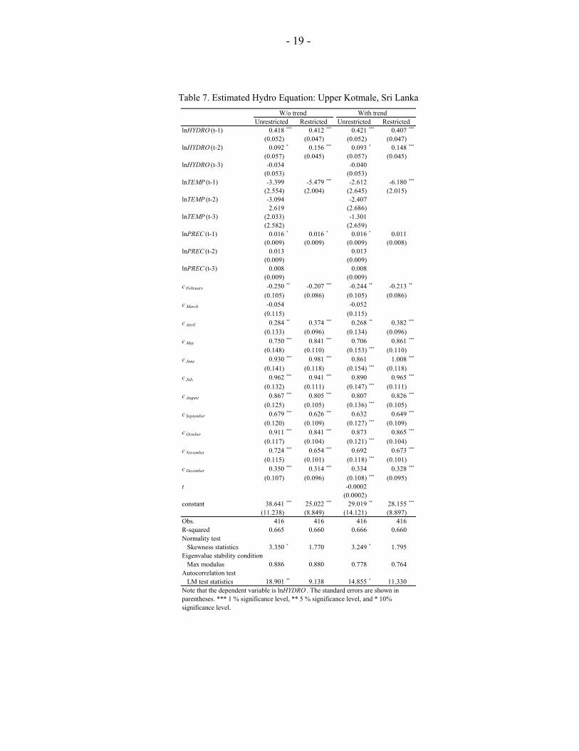
Tables 7 and 8 show the VAR estimates of the hydrological equation for the Upper Kotmale

and Thac Mo cases, respectively. Similar to the above, the hydrological discharge in the

Kotmale River would increase with rainfall and decrease with temperature. In this case,

however, temperature seems to have a much more powerful effect than precipitation. It is

also shown that the deterministic rainy season appears much long—from April to

December—at least when inferring from hydrology.

By contrast, the monthly discharge at the Thac Mo Reservoir may be less related to

temperature and precipitation in a statistical sense; both coefficients are insignificant. Rather,

the river flow is determined by only its own lagged values and deterministic seasonality.

Interestingly, in addition, the Ba River may have a positive time trend, meaning that the

amount of available water would become larger as time rolls on, in spite of seasonality and

stochastic changes.

- 18 -

Table 6. Estimated Hydro Equation: Vishnugad Pipalkoti, India

Unrestricted UnrestrictedlnHYDRO (t-1) 1.072 *** 1.093 *** 1.066 *** 1.094 ***

(0.064) (0.054) (0.065) (0.054)lnHYDRO (t-2) -0.209 *** -0.251 *** -0.212 *** -0.249 ***

(0.068) (0.059) (0.068) (0.059)lnTEMP (t-1) -0.817 ** -0.671 *** -0.849 *** -0.681 ***

(0.374) (0.238) (0.375) (0.238)lnTEMP (t-2) 0.236 0.204

(0.352) (0.354)lnPREC (t-1) -0.003 -0.003

(0.003) (0.003)lnPREC (t-2) 0.008 ** 0.007 ** 0.009 *** 0.007 **

(0.003) (0.003) (0.003) (0.003)c February 0.018 0.008

(0.087) (0.087)c March 0.233 ** 0.181 *** 0.218 *** 0.183 ***

(0.093) (0.069) (0.095) (0.069)c April 0.656 *** 0.590 *** 0.645 *** 0.594 ***

(0.104) (0.078) (0.104) (0.078)c May 1.168 *** 1.108 *** 1.168 *** 1.111 ***

(0.130) (0.100) (0.130) (0.100)c June 0.944 *** 0.908 *** 0.960 *** 0.911 ***

(0.162) (0.110) (0.162) (0.111)c July 0.810 *** 0.811 *** 0.834 *** 0.812 ***

(0.170) (0.091) (0.172) (0.091)c August 0.419 ** 0.442 *** 0.446 *** 0.441 ***

(0.168) (0.076) (0.171) (0.076)c September 0.077 0.104

(0.161) (0.164)c October -0.228 -0.205

(0.150) (0.152)c November 0.021 0.036

(0.127) (0.128)c December -0.079 -0.069

(0.093) (0.093)t 0.0001

(0.0001)constant 2.758 * 3.230 *** 3.020 * 3.254 ***

(1.674) (0.807) (1.697) (0.807)Obs. 238 238 238 238R-squared 0.951 0.946 0.951 0.946Normality test Skewness statistics 6.764 *** 4.900 ** 4.313 ** 5.053 **

Eigenvalue stability condition Max modulus 0.739 0.765 0.752 0.770Autocorrelation test LM test statistics 18.695 ** 10.293 20.031 ** 10.532Note that the dependent variable is lnHYDRO . The standard errors are shown in parentheses. *** 1 % significance level, ** 5 % significance level, and * 10% significance level.

Restricted RestrictedW/o trend With trend

- 19 -

Table 7. Estimated Hydro Equation: Upper Kotmale, Sri Lanka


(0.052) (0.047) (0.052) (0.047)lnHYDRO (t-2) 0.092 * 0.156 *** 0.093 * 0.148 ***

(0.057) (0.045) (0.057) (0.045)lnHYDRO (t-3) -0.034 -0.040

(0.053) (0.053)lnTEMP (t-1) -3.399 -5.479 *** -2.612 -6.180 ***

(2.554) (2.004) (2.645) (2.015)lnTEMP (t-2) -3.094 -2.407

2.619 (2.686)lnTEMP (t-3) (2.033) -1.301

(2.582) (2.659)lnPREC (t-1) 0.016 * 0.016 * 0.016 * 0.011

(0.009) (0.009) (0.009) (0.008)lnPREC (t-2) 0.013 0.013

(0.009) (0.009)lnPREC (t-3) 0.008 0.008

(0.009) (0.009)c February -0.250 ** -0.207 *** -0.244 ** -0.213 **

(0.105) (0.086) (0.105) (0.086)c March -0.054 -0.052

(0.115) (0.115)c April 0.284 ** 0.374 *** 0.268 ** 0.382 ***

(0.133) (0.096) (0.134) (0.096)c May 0.750 *** 0.841 *** 0.706 0.861 ***

(0.148) (0.110) (0.153) *** (0.110)c June 0.930 *** 0.981 *** 0.861 1.008 ***

(0.141) (0.118) (0.154) *** (0.118)c July 0.962 *** 0.941 *** 0.890 0.965 ***

(0.132) (0.111) (0.147) *** (0.111)c August 0.867 *** 0.805 *** 0.807 0.826 ***

(0.125) (0.105) (0.136) *** (0.105)c September 0.679 *** 0.626 *** 0.632 0.649 ***

(0.120) (0.109) (0.127) *** (0.109)c October 0.911 *** 0.841 *** 0.873 0.865 ***

(0.117) (0.104) (0.121) *** (0.104)c November 0.724 *** 0.654 *** 0.692 0.673 ***

(0.115) (0.101) (0.118) *** (0.101)c December 0.350 *** 0.314 *** 0.334 0.328 ***

(0.107) (0.096) (0.108) *** (0.095)t -0.0002

(0.0002)constant 38.641 *** 25.022 *** 29.019 ** 28.155 ***

(11.238) (8.849) (14.121) (8.897)Obs. 416 416 416 416R-squared 0.665 0.660 0.666 0.660Normality test Skewness statistics 3.350 * 1.770 3.249 * 1.795Eigenvalue stability condition Max modulus 0.886 0.880 0.778 0.764Autocorrelation test LM test statistics 18.901 ** 9.138 14.855 * 11.330Note that the dependent variable is lnHYDRO . The standard errors are shown in parentheses. *** 1 % significance level, ** 5 % significance level, and * 10% significance level.


- 20 -

Table 8. Estimated Hydro Equation: Thac Mo, Vietnam


(0.056) (0.030) (0.060) (0.030)lnTEMP (t-1) 2.145 0.849

(1.520) (1.607)lnPREC (t-1) 0.097 0.111

(0.145) (0.144)c February -0.158 -0.207

(0.175) (0.174)c March -0.124 -0.172

(0.241) (0.239)c April 0.057 -0.096

(0.232) (0.239)c May 0.713 *** 1.041 *** 0.728 *** 1.022 ***

(0.220) (0.093) (0.218) (0.093)c June 1.231 *** 1.581 *** 1.300 *** 1.575 ***

(0.178) (0.086) (0.179) (0.085)c July 1.517 *** 1.762 *** 1.648 *** 1.773 ***

(0.189) (0.088) (0.196) (0.088)c August 1.820 *** 1.958 *** 1.996 *** 1.981 ***

(0.206) (0.099) (0.217) (0.099)c September 1.525 *** 1.567 *** 1.747 *** 1.602 ***

(0.231) (0.113) (0.248) (0.113)c October 1.237 *** 1.271 *** 1.424 *** 1.307 ***

(0.242) (0.116) (0.253) (0.116)c November 0.478 ** 0.518 *** 0.630 *** 0.551 ***

(0.238) (0.112) (0.245) (0.112)c December 0.095 0.163

(0.188) (0.188)t 0.0008 ** 0.0007 **

(0.0003) (0.0003)constant -8.273 0.779 *** -2.804 0.634 ***

(6.550) (0.122) (6.907) (0.146)Obs. 239 239 239 239R-squared 0.947 0.943 0.948 0.944Normality test Skewness statistics 31.928 *** 21.081 *** 28.797 *** 19.477 ***

Eigenvalue stability condition Max modulus 0.536 0.657 0.471 0.642Autocorrelation test LM test statistics 7.404 16.901 * 4.209 12.995Note that the dependent variable is lnHYDRO . The standard errors are shown in parentheses. *** 1 % significance level, ** 5 % significance level, and * 10% significance level.


Long-term time trends

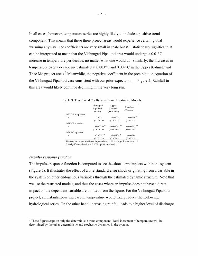
From the long-term perspective, it is of particular interest whether the system involves a time

trend component. Table 9 summarizes the trend coefficients in each unrestricted model. As

touched upon in the above, only the hydrological series at the Thac Mo Reservoir has a

positive and significant time trend among our sample projects.

- 21 -

In all cases, however, temperature series are highly likely to include a positive trend

component. This means that these three project areas would experience certain global

warming anyway. The coefficients are very small in scale but still statistically significant. It

can be interpreted to mean that the Vishnugad Pipalkoti area would undergo a 0.01°C

increase in temperature per decade, no matter what one would do. Similarly, the increases in

temperature over a decade are estimated at 0.003°C and 0.009°C in the Upper Kotmale and

Thac Mo project areas.7 Meanwhile, the negative coefficient in the precipitation equation of

the Vishnugad Pipalkoti case consistent with our prior expectation in Figure 5. Rainfall in

this area would likely continue declining in the very long run.

Table 9. Time Trend Coefficients from Unrestricted Models


Upper Kotmale

(Sri Lanka)

Thac Mo (Vietnam)

lnHYDRO equation: t 0.00011 -0.00021 0.00079 **

(0.00013) (0.00018) (0.00035)lnTEMP equation: t 0.000050 ** 0.000015 *** 0.000042 ***

(0.000023) (0.000004) (0.000014)lnPREC equation: t -0.00517 * -0.00178 * -0.00016

(0.00272) (0.00098) (0.00015)The standard errors are shown in parentheses. *** 1 % significance level, ** 5 % significance level, and * 10% significance level.

Impulse response function

The impulse response function is computed to see the short-term impacts within the system

(Figure 7). It illustrates the effect of a one-standard error shock originating from a variable in

the system on other endogenous variables through the estimated dynamic structure. Note that

we use the restricted models, and thus the cases where an impulse does not have a direct

impact on the dependent variable are omitted from the figure. For the Vishnugad Pipalkoti

project, an instantaneous increase in temperature would likely reduce the following

hydrological series. On the other hand, increasing rainfall leads to a higher level of discharge.

7 These figures capture only the deterministic trend component. Total increment of temperature will be determined by the other deterministic and stochastic dynamics in the system.

- 22 -

The system seems to have a relatively long adjustment process; a given shock will disappear

after more than one year.

The Kotmale River hydrology follows the same story. If it rains more, the water flow would

increase. If it is hotter than usual, then the river tends to be lean. In the case of the Thac Mo

hydropower project, the restricted models have no direct impact of climate changes on

hydrology. Accordingly, these impulse response functions are not presented.

- 23 -

Figure 7. Impulse Response Function

(Vishnugad Pipalkoti, India)

0

.5

1

1.5

0 10 20 30step

lnHYDRO->lnHYDRO

-1.5

-1

-.5

0

0 10 20 30step

lnTEMP->lnHYDRO

0

.5

1

0 10 20 30step

lnTEMP->lnTEMP

0

.005

.01

.015

0 10 20 30step

lnPREC->lnHYDRO

0

.001

.002

.003

0 10 20 30step

lnPREC->lnTEMP

(Upper Kotmale, Sri Lanka)

0

.5

1

0 10 20 30step

lnHYDRO->lnHYDRO

-10

-5

0

0 10 20 30step

lnTEMP->lnHYDRO

0

.5

1

0 10 20 30step

lnTEMP->lnTEMP

0

.01

.02

.03

0 10 20 30step

lnPREC->lnHYDRO

-.0006

-.0004

-.0002

0

0 10 20 30step

lnPREC->lnTEMP

(Thac Mo, Vietnam)

0

.5

1

0 10 20 30step

lnHYDRO->lnHYDRO

0

.02

.04

.06

.08

0 10 20 30step

lnHYDRO->lnPREC

0

.5

1

0 10 20 30step

lnTEMP->lnTEMP

0

1

2

3

0 10 20 30step

lnTEMP->lnPREC

-2.000e-18

0

2.000e-18

4.000e-18

0 10 20 30step

lnPREC->lnTEMP

-.5

0

.5

1

0 10 20 30step

lnPREC->lnPREC

- 24 -

Causality

Causality tests are one of the advantages of estimating a multivariate stochastic system; this

feature cannot be used when analyzing only a univariate hydrological time series or imposing

the meteorological or physical hydrologic relationship in advance. The conventional Granger

causality test can reveal what causes what. In the Vishnugad Pipalkoti case, temperature

Granger-causes water flow of the Alaknanda River (Table 10). The null hypothesis that

temperature is irrelevant in the hydro equation can be rejected at the 10 percent significance

level, and the hypothesis of hydrology being unimportant to determine temperature cannot be

rejected. In the same manner, rainfall also Granger-causes the river flow.

By contrast, at the Kotmale River, temperature seems to cause the water level, and vice

versa. The null hypothesis that temperature influences hydrology cannot be rejected, but at

the same time, the hypothesis of hydrological series being critical in the temperature equation

can also be accepted. Statistically, rainfall does not cause hydrology.

Finally, in the Thac Mo case there is no conclusive causal relationship between climate and

hydrology, though temperature Granger-causes precipitation in the region. In sum,

hydrological series are likely to be impacted on by climate changes, particularly temperature.

However, it may vary on a case-by-case basis.

Table 10. Causality Test

Null hypothesislnTEMP => lnHYDRO 4.789 * 11.508 *** 1.990lnPREC => lnHYDRO 6.935 ** 5.788 0.450lnHYDRO => lnTEMP 4.046 6.485 * 0.003lnPREC => lnTEMP 4.077 3.816 0.321lnHYDRO => lnPREC 0.427 1.364 1.928lnTEMP => lnPREC 2.159 1.554 12.665 ***

*** 1 % significance level, ** 5 % significance level, and * 10% significance level.


Upper Kotmale

(Sri Lanka)

Thac Mo (Vietnam)

Chi2 statistics

Chi2 statistics

Chi2 statistics

- 25 -

V. DISCUSSION

Hydrological forecasts

What does the above mean from a hydropower project perspective? First, it means that future

hydrological series may be different from what one envisages at the project preparation stage.

In ex ante assessing a hydropower project, it is broadly common that the 90 percent

dependable hydrological level—which is referred to as a baseline hereinafter—is used as a

forecast of water flow available in the future. It is a very conservative approach, which is

high-principled for cautious project preparation purposes. However, it is worth recalling that

this is just one of the univariate nonparametric point estimates, leaving most hydrological

information unused.8

As shown in Figure 8, the hydrological forecasts in 2025 based on our empirical results in

fact look very different from data in the conventional 90 percent dependable year. The figure

includes two types of forecasts: One is the dynamic forecasts, which are calibrated from the

last observation in the sample, following the estimated system of equations. The other is one-

step-ahead projections, which are calculated by fitting a set of values for the estimated

equations to obtain the predicted values in the next period. In this regard the IPCC forecasts

presented in Table 2 are adopted as a reference point.9

In both Vishnugad Pipalkoti and Thac Mo cases, the rainy season would have higher levels

of water than the baselines.10 However, in the lean season water resources may become even

more limited. For the Upper Kotmale project, the river would have a greater flow of water

almost all the year around. Our dynamic forecasts look more prone to be greater than the

one-step-ahead projections. The reason is that the long-run calibration is very sensitive to

8 It is a separate question whether the past hydrological time series contain useful information. 9 The dynamic forecasts tend to have much large standard errors, due to the nature of the estimation method. Since we are computing the 240-period-ahead projections, the standard errors are amplified quickly. 10 Again, the baseline is a conservative assumption, which is the 10th percentile estimate. On the other hand, our dynamic estimate is, roughly speaking, calculated on a mean basis, as usual.

- 26 -

changes in parameter estimates; a small change in the coefficients could yield a very different

picture of the future. Notably, however, the difference between the dynamic forecasts and

one-step-ahead projections is relatively tolerable in any time series.

Figure 8. Monthly Hydrological Forecasets, 2025

(Million m3 per month)

(Vishnugad Pipalkoti, India) (Upper Kotmale, Sri Lanka)

0

200

400

600

800

1000

1200

Jun Jul Aug Sep Oct Nov Dec Jan Feb Mar Apr May

90% dependable yearDynamic forecastsOne-step-ahead projections (based on IPCC)

0

10

20

30

40

50

60

70

Oct Nov Dec Jan Feb Mar Apr May Jun Jul Aug Sep


(Thac Mo, Vietnam)

0

100

200

300

400

500

600

700

800

Jan Feb Mar Apr May Jun Jul Aug Sep Oct Nov Dec


Impacts on power generation

To focus on the effect of climate changes while controlling for the existing difference in

project design, objective and operation, suppose that all plants provide base load energy,

meaning that they always operate as long as water resources are available. The individual

- 27 -

physical characteristics of plants hold constant, such as installed capacity and net head. The

baseline scenario also assumes that there is no major storage capacity.11

Without large storage capacity, just like the Vishnugad Pipalkoti project, the implication of

changing hydrological series is direct. If the level of river flow is above the maximum design

water discharge of the power station, there is no impact at least in terms of the amount of

energy generated.12 For instance, the design discharge of VPHEP is 224 m3 per second or

about 580 million m3 per month. Thus, the possible large increase in hydrology from June to

August in 2025 could not be exploited for power generation purposes. Rather, in the lean

season the power station would likely be faced with a severer water constraint.

Table 11 shows the predicted impacts of climate changes on electricity generation. The

amount of energy is calculated on a monthly basis in each scenario, and annual energy is the

summation of monthly values. Due to increased river discharges during the early and late

rainy season, the Vishnugad Pipalkoti power station would be able to generate more energy

in 2025. However, this increment may be relatively modest at about 7.5 percent. The impact

of decreased water in the lean flow season would be marginal, because the baseline scenario

has already taken into account the fact that the Alaknanda River even now has the very low

level of water flow during the lean season. Because of lack of sufficient storage capacity, the

Vishnugad Pipalkoti power station will not fully take advantage of water resources available

in the high-water season.

In the Upper Kotmale case, a projected increase in water flow may allow to generate about

45 percent more energy than the baseline level. Significantly, this is because the installed

capacity is large enough to absorb increasing water flow. Still, the load factor will be

estimated at about 40 percent. Although the large installed capacity of the Upper Kotmale

11 For simplicity, it is also assumed that the total utilization rate of installed capacity is 95 percent. In addition, the combined turbine and generator efficiency is commonly assumed 93 percent. 12 Extreme events induced by increased variability and seasonality are a different issue and beyond the scope of this sturdy. This paper is analyzing hydrological series merely on the monthly mean level.

- 28 -

hydropower station is intended to supply peak energy given storage for a few days, it might

have the additional advantage of exploiting increased hydrological resources for power

generation.13 It will also exhibit certain resistance to increased variability in water flow and

extreme events.

Provided that the large-scale reservoir is not used, annual energy generated by the Thac Mo

power station might decline given the 2025 hydrological dynamic forecasts. The expected

water flow has a large volatility and cannot be absorbed by its relatively small installed

capacity of 75 MW. The negative impact of lower water levels in the dry season would be

dominant in this case.

In reality, however, these hydro stations have storage capacities to a greater or lesser extent.

Only the Thac Mo project has a large-scale reservoir of 1,250 million m3 for about six

months. Recall that the station is intended to supply peak load energy. The Upper Kotmale,

which also aims at providing three-hour peak energy, has only a daily storage. The

Vishnugad Pipalkoti project has an hourly storage.

The benefit from a large-scale reservoir is apparent in our monthly-based analytical

framework. Under the assumption of the maximum use of the existing storage capacity, the

Thac Mo hydropower station would be able to increase to 524 GWh from 383 GWh of the

baseline case.14 This implies that having a storage capacity is useful for accommodating

increased seasonality in hydrological series. The Vishnugad Pipalkoti project does not benefit

from such seasonal variation adjustment, because its storage capacity is small. The Upper

Kotmale hydropower plant does not benefit either; but this is because its installed capacity is

large enough to use all the flow of the Kotmale River, even if it increases.

13 Note that the storage capacity attached to the Upper Kotmale power station is too small to influence the current discussion. 14 The assumed operating rule of the storage capacity is this: extra water is stored in a reservoir whenever the available water flow exceeds the hydroplant deign discharge. When the available water is insufficient, the stored water is used for generation as long as there is water.

- 29 -

Table 11. Impact of Changes in Hydrology on Electricity Generation

Baseline Dynamic forecast (2025)



Dynamic forecast (2025)

Annual energy (GWh) 1,768 1,898 357 522 383 331 524Storage capacity assumption No No No No No No Yes

Memorandum items: Installed capacity (MW) 440 440 150 150 75 75 75Monthly available capacity (MW)

Average 212 280 46 67 48 44 62Maximum 440 440 107 94 75 75 75Minimum 70 63 6 24 10 5 5

Average available water flows (m3/sec) 115 156 10 14 83 88 81Net head (m) 205 205 473 473 90 90 90Intended power generation operations Base Base Base Base Base Base Base

Source: Author's estimates. Note: The baseline scenario assumes hydrological series in a 90 percent dependable year.


Upper Kotmale (Sri Lanka)

Thac Mo (Vietnam)

Impacts on project viability assessment

As annual energy changes, the economic and financial project viability might also change.

Table 12 presents the internal rate of return (IRR) corresponding to each scenario. For

simplicity, it is assumed that the project cost is distributed evenly for the first five years

before the following 30-year operation. Annual operation and maintenance costs are set at

1.5 percent of total project costs. The price (or benefit) of energy generated is assumed 7 U.S.

cents per kWh in all cases, despite the fact that it varies across countries and across types of

customers. This is just for comparison purposes. It is worth noting that peak load energy

should be estimated to be economically more valuable in reality. No other economic benefits

and costs are accounted for. Finally, the climate change scenario assumes that the baseline

hydro energy is used for the first 10 years of operation, and the estimated dynamic forecasts

are applied afterwards.

The economic effect of changes in energy generated has been found relatively small contrary

to prior expectations. This is mainly attributable to our assumption that climate changes

would realize 10 years after the power station commissioning. For the Vishnugad Pipalkoti

project, climate changes would increase the IRR by only 0.3 percentage points. In the Thac

Mo case, a changing climate might lower the IRR, but with its attached reservoir the rate of

- 30 -

return would increase from 28.8 percent to 29.6 percent. However, provided that climate

changes affect hydrology from the beginning of the plant operation, the rate of return to the

Thac Mo project would rise to about 35 percent. This may indicate a pitfall in assessing a

hydropower project in economic terms; the future climate change impacts are generally

underestimated in the IRR calculation, even though they are environmentally and socially

significant.

In the Upper Kotmale case, a substantial increase in electricity production could be expected

because of its margin of installed capacity, resulting in a higher IRR of 6.4 percent. The

existing daily storage does not directly affect this result. These pieces of evidence suggest

that having larger installed capacity and some storage capacity might be well worth

consideration.

Table 12. Impact of Changes in Hydrology on Internal Rate of Return

Without storage

With current storage Baseline Dynamic

forecasts (2025)

Vishnugad Pipalkoti (India) 15.8% 16.1% 16.1% 10.9% 11.9%Upper Kotmale (Sri Lanka) 4.7% 6.4% 6.4% 1.2% 3.2%Thac Mo (Vietnam) 29.0% 28.8% 29.6% 21.9% 22.6%Source: Author's estimates.

50% additional project cost

Note: The baseline scenario assumes hydrological series in a 90 percent dependable year without major storage capacity.

Original project costDynamic forecasts (2025)

Baseline

for a 6-month storage capacity

Importantly, the above discussion does ignore the likely implication on the cost side. Larger

installed capacity must of necessity bring about higher construction costs. If a large-scale

storage capacity is planned, the additional costs would be enormous not only financially but

also socially. For example, consider a 50 percent increase in total project costs for

constructing a six month storage capacity. The optimal size of reservoir ranges from several

hours to over a year, depending on geological and environmental conditions and operational

objectives. The storage capacity selected here is roughly equivalent to the gross storage at the

full reservoir level of the Thac Mo Reservoir. Note that in the Thac Mo case the project cost

does not include any fraction of past investment in the original Thac Mo Reservoir; thus, this

additional cost scenario may still be meaningful even in the Thac Mo case.

- 31 -

As shown in the last two columns of Table 12, the project viability is much more sensitive to

the presumed cost increase rather than changing hydrological flows. An additional

investment cost would dramatically lower the IRRs. For instance, the rate of return for the

Vishnugad Pipalkoti project drops by 5 percentage points under the baseline assumption.

Given our estimated hydrological forecasts, the project viability could improve to a certain

extent, thanks to the leveled hydrological series by the additional storage capacity. However,

such benefits may not be fully justifiable from the IRR perspective. It depends on the cost.

Notably, in fact, such a large-scale reservoir has been found overinvestment in the Vishnugad

Pipalkoti case; probably a 2-3 month reservoir might be sufficient to follow our hypothetical

operating rule of the storage. Thus, larger generation and storage capacities may be a

measure against uncertain climate changes; but these options may be expensive, and the

potential environmental and social costs could also be considerable.15 A broad and consistent

evaluation will be needed for further assessment.

Limitation of the model

The above discussion has several limitations. First of all, the hydrological projections might

be underestimated, because they are essentially estimated based on the past climate and

hydrological time series. Including more time series observation contributes to improving

statistical reliability but risks underestimating the recent trend in river runoff and climate

variables.

15 The development of international support mechanisms for climate change adaptation seems to be lagging behind climate change mitigation. Adaptation measures are mostly considered private goods, while mitigation efforts can be rewarded through the growing carbon market, due to their perceived positive global externalities. In the case of hydropower, however, there are synergies between the adaptation and mitigation agendas: additional installed generation or reservoir capacities could help to adapt to expected changes in river flows and also result in increased production of electricity with low/zero carbon emissions, replacing carbon-intensive power generation.

- 32 -

Second, despite their potential significance, the impact of extreme events is not captured in

the above model because of both data and methodological limitations. As shown in Figure 5,

for example, the Alaknanda hydrological series appears to have become more volatile in

recent years. However, the analysis based on monthly data cannot explain extreme events,

such as flash floods and rain floods caused by extremely heavy precipitation in a few days.16

Any econometric technique is more or less designed to measure an average effect, ignoring

outliers like floods and droughts.

Notably, though, the above projections are still considered suggestive. For example, it can be

shown that in the Vishnugad Pipalkoti case the skewness of a monthly water flow

distribution is likely to increase from 0.74 to 1.02 by the 2020s. Generally, Figure 8 also

indicates a considerable increase in water flows particularly during the rainy season in all

cases. Especially for the Vishnugad Pipalkoti hydropower project, in comparison with the

designed capacity the projected surge in river discharge may not be ignorable from the point

of view of flood and sediment risk management.

Third, one might question whether the stochastic model is generally suitable for this type of

study. It is open to discussion. The above analysis finds the hydrological series at the Thac

Mo Reservoir may exhibit a unit root and thus not be applicable to the VAR technique.17

When detrended data are used, the result has been found quite similar to the result presented

above. Nonetheless, even if the model is appropriate, there is another level of problem. For

example, Wong et al. (2007) claims that the assumption of a river flow linearly depending on

its lagged values is questionable. Our VAR model does not rely on the linearity restriction,

but it is simply a log-linear model, which still imposes certain restrictions on the system, e.g.,

constant elasticity.

16 Technically, it may be somewhat meaningful to predict the extreme river flows based on our estimated standard error. For instance, the predicted flows at the 90 percent dependable level—meaning an upper bound of the less significant interval—could be interpreted as a very unlikely flood event in a statistical sense. 17 If all time series in the system contain a unit root, the vector error-correction model is more appropriate.

- 33 -

In addition, some variables that are critically related to hydrological flows may be omitted

from our model. Bergström et al. (2001) point out that a key to successful hydrological

modeling is to properly account for soil moisture, which is not included in the above model.

There are possibly other omitted variables. In the context of Northern India, for instance, the

retreating Himalayan glaciers may have to be taken into consideration.18 However, there may

be a tradeoff; more variables will involve more uncertainty. Particularly, evapotranspiration

in a future clime may involve serious uncertainty to be modeled (Bergström et al., 2001).

Mountain areas where hydropower projects are often located may be more complicated

because mountains are among the most fragile environments; the rate of warming in

mountain systems is expected to be two to three times higher than that recorded during the

20th century (Nogués-Bravo et al., forthcoming).

There is a piece of evidence to support the validity of the used stochastic model. When

comparing our dynamic forecasts of temperature and precipitation with the IPCC projections,

temperature forecasts seem well comparable (Figure 9). On the other hand, precipitation

forecasts are broadly consistent but may be underestimated in some cases, such as the

Vishnugad Pipalkoti project. The difference may be attributed to the factors that the IPCC

model accounts for and our VAR model does not. Obviously, again, the IPCC projections, as

such, may have to be interpreted with some caution.

18 The Himalayan glaciers are currently retreating at a speed of 10-15 meters a year (WWF Nepal Program, 2005).

- 34 -

Figure 9. Predicted Climate Changes, Comparing between IPCC and Dynamic Forecasts, 2025

Vishnugad Pipalkoti, India

(Temperature; °C) (Precipitation; mm/month)

0

5

10

15

20

25

30

35


Dynamic forecastsIPCC projections

0

50

100

150

200

250

300

350

400

450



Upper Kotmale, Sri Lanka


0

5

10

15

20

25

30

35



0

50

100

150

200

250

300

350

400

450



Thac Mo, Vietnam


0

5

10

15

20

25

30

35



0

50

100

150

200

250

300

350

400

450



- 35 -

Finally, the climate forecasts may need refining furthermore in terms of spatial

representation. The above discussion partly depends on the global climate change model for

one-step-ahead climate projections. Ideally, however, the basin-level climate forecasts would

be more appropriate input (e.g., Kothyari and Singh, 1996; Pant and Kumar, 1997; Lal and

Aggarwal, 2001). The above analytical framework implicitly assumes that temperature and

precipitation data at or close to the project site could represent all climate conditions over the

upper basin—e.g., surface water, groundwater and soil moisture—that would result in flow at

the dam location. This may not always hold. At the same time, however, if all the

relationship were modeled in a physical hydrologic manner, there would be no room where

the statistical hydrology approach could be performed, because there would be no degree of

freedom. In other words, a missing gap that should be bridged is, to my best knowledge, the

comparison between those two approaches. A further research will be needed to answer

whether or not they are compatible and which is better if not.

VI. CONCLUSION

The world economy is now faced with considerable risk and uncertainty caused by climate

changes. Increasing attention has been paid to hydropower generation in recent years,

because it is renewable energy. However, hydropower is one of the industries that would be

most likely to be affected by changes in global and regional climate. The paper applies a

hydrological model using a VAR technique to three hydropower projects in India, Sri Lanka

and Vietnam.

The possible climate change impacts have rarely been evaluated in an explicit manner when a

hydropower project is ex ante assessed in economic terms. Conventionally, the 90 percent

dependable hydrological level is used as a forecast of water flow in the future. However, it is

shown that the hydrological forecasts calibrated from the empirical VAR models are very

different from the conventional projections.

- 36 -

The climate change impacts in principal differ from location to location; but as far as the

selected three projects are concerned, hydrological discharges tend to increase with rainfall

and decrease with temperature. It is also shown that the rainy season would likely have

higher water levels, but in the lean season water resources would become even more limited.

The resultant effect on project viability may be modest at best, largely because of the

calculus nature of discounting possible costs and benefits in the future. However, when

comparing the three cases, it is indicated that having larger installed capacity might be useful

to exploit increased hydrological resources for power generation. Also, hydropower stations

with some storage capacities may have the advantage of accommodating increased

seasonality in hydrological series. However, these may not be able to be overgeneralized,

because the paper investigates only three cases. More case studies are necessary for drawing

general implications, such as hydropower design alternatives.

Nonetheless, these mitigation measures against uncertain climate changes must have a cost

implication in economic and social terms. Hence, a broad and consistent assessment will be

needed at the project preparation stage.

- 37 -

REFERENCE

Akaike, Hirotugu. 1973. Information theory and an extension of the maximum likelihood principle, in Second International Symposium on Information Theory, eds. by B. N. Petrov and F. Csaki, pp. 267-281, Académiai Kiadó, Budapest.

Bergström, Sten, Bengt Carlsson, Marie Gardelin, Göran Lindeström, Anna Pettersson, Markku Rummukainen. 2001. Climate change impacts on runoff in Sweden—assessments by global climate models, dynamical downscaling and hydrological modeling. Climate Research, Vol. 16, pp. 101-112.

Bhunya, P.K., R. Berndtsson, C.S.P. Ojha, S.K. Mishra. 2007. Suitability of gamma, chi-square, weibull, and beta distributions as synthetic unit hydrographs. Journal of Hydrology, Vol. 334, pp. 28-38.

Goswami, B.N., V. Venugopal, D. Sengupta, M.S. Madhusoodanan, P.K. Xavier. 2006. Increasing trend of extreme rain events over India in a warming environment. Science, Vol. 314, pp. 1442-1445.

Kay, Alison, Richard Jones, Nicholas Reynard. 2006. RCM rainfall for UK flood frequency estimation. II. Climate change results. Journal of Hydrology, Vol. 318, pp. 163-172.

Khaliq, M.N., T.B.M.J. Ouarda, J.-C. Ondo, P. Gachon, B. Bobée. 2006. Frequency analysis of a sequence of dependent and/or non-stationary hydro-meteorological observations: a review. Journal of Hydrology, Vol. 329, pp. 534-442.

Koutsoyiannis, Demetris. 2006. Nonstationarity versus scaling in hydrology. Journal of Hydrology, Vol. 324, pp. 239-254.

Lettenmaier, Dennis, Eric Wood. 1993. Hydrologic forecasting, in Handbook of Hydrology, eds. by David Maidment, pp. 19.1-19.72, McGraw-Hill, Inc., New York.

Malamud, Bruce, Donald Turcotte. 2006. The applicability of power-law frequency statistics to floods. Journal of Hydrology, Vol. 322, pp. 168-180.

O’Connell, Daniel. 2005. Nonparametric Bayesian flood frequency estimation. Journal of Hydrology, Vol. 313, pp. 79-96.

Salas, Jose. 1993. Analysis and modeling of hydrologic time series, in Handbook of Hydrology, eds. by David Maidment, pp. 19.1-19.72, McGraw-Hill, Inc., New York.

Samaniego, Luis, András Bárdossy. 2007. Relating macroclimatic circulation patterns with characteristics of floods and droughts at the mesoscale. Journal of Hydrology, Vol. 335, pp. 109-123.

Shalizi, Zmarak. 2007. Energy and emissions: local and global effects of the rise of China and India. Policy Research Working Paper No. 4209, the World Bank.

Stedinger, Jery, Richard Vogel, Efi Foufoula0Georgiou. 1993. Frequency analysis of extreme events, in Handbook of Hydrology, eds. by David Maidment, pp. 18.1-18.66, McGraw-Hill, Inc., New York.

- 38 -

World Bank. 2007. Addressing climate change-driven increased hydrological variability in environmental assessments for hydropower projects—a scoping study. Mimeograph.

Wong, Heung, Wai-cheung Ip, Riquan Zhang, Jun Xia. 2007. Hon-parametric time series models for hydrologic forecasting. Journal of Hydrology, Vol. 332, pp. 337-347.

Documents

Estimating Global Climate Change Impacts on Hydropower