Embed Size (px)
Citation preview

2004
TRC9804
ERSA Wheel-Track Testing for
Rutting and Stripping
Stacy G. Williams, Kevin D. Hall
Final Report


FINAL REPORT
TRC-9804
ERSA Wheel Track Testing for Rutting and Stripping
by
Stacy G. Williams and Kevin D. Hall
Conducted by
Department of Civil Engineering University of Arkansas
In cooperation with
Arkansas State Highway and Transportation Department
US Department of Transportation Federal Highway Administration
University of Arkansas Fayetteville, Arkansas 72701
March 2004
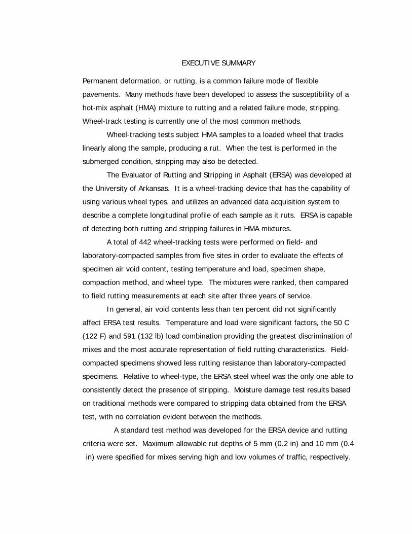
EXECUTIVE SUMMARY
Permanent deformation, or rutting, is a common failure mode of flexible
pavements. Many methods have been developed to assess the susceptibility of a
hot-mix asphalt (HMA) mixture to rutting and a related failure mode, stripping.
Wheel-track testing is currently one of the most common methods.
Wheel-tracking tests subject HMA samples to a loaded wheel that tracks
linearly along the sample, producing a rut. When the test is performed in the
submerged condition, stripping may also be detected.
The Evaluator of Rutting and Stripping in Asphalt (ERSA) was developed at
the University of Arkansas. It is a wheel-tracking device that has the capability of
using various wheel types, and utilizes an advanced data acquisition system to
describe a complete longitudinal profile of each sample as it ruts. ERSA is capable
of detecting both rutting and stripping failures in HMA mixtures.
A total of 442 wheel-tracking tests were performed on field- and
laboratory-compacted samples from five sites in order to evaluate the effects of
specimen air void content, testing temperature and load, specimen shape,
compaction method, and wheel type. The mixtures were ranked, then compared
to field rutting measurements at each site after three years of service.
In general, air void contents less than ten percent did not significantly
affect ERSA test results. Temperature and load were significant factors, the 50 C
(122 F) and 591 (132 lb) load combination providing the greatest discrimination of
mixes and the most accurate representation of field rutting characteristics. Field-
compacted specimens showed less rutting resistance than laboratory-compacted
specimens. Relative to wheel-type, the ERSA steel wheel was the only one able to
consistently detect the presence of stripping. Moisture damage test results based
on traditional methods were compared to stripping data obtained from the ERSA
test, with no correlation evident between the methods.
A standard test method was developed for the ERSA device and rutting
criteria were set. Maximum allowable rut depths of 5 mm (0.2 in) and 10 mm (0.4
in) were specified for mixes serving high and low volumes of traffic, respectively.

TABLE OF CONTENTS
List of Tables ................................................................................................. ix
List of Figures............................................................................................... xii
List of Acronyms ..........................................................................................xvii
Chapter 1 – Introduction .................................................................................1
Introduction ...........................................................................................2
Asphalt Mixture Design ...........................................................................3
Marshall Mixture Design ..................................................................3
Hveem Mixture Design....................................................................5
Superpave......................................................................................6
Chapter 2 – Background................................................................................ 11
Flexible Pavement Distresses................................................................. 12
Low Temperature Cracking ........................................................... 12
Fatigue Cracking........................................................................... 15
Permanent Deformation ................................................................ 21
Permanent Deformation Tests ....................................................... 30
Moisture Susceptibility .................................................................. 34
Moisture Susceptibility Tests.......................................................... 38
Wheel-Tracking Tests............................................................................ 48
Hamburg Wheel-Tracking Device................................................... 49
French Rut Tester......................................................................... 52
Georgia Loaded Wheel Test .......................................................... 53
Asphalt Pavement Analyzer ........................................................... 55

Accelerated Loading Facility .......................................................... 58
Model Mobile Load Simulator......................................................... 59
Superfos Construction Rut Tester .................................................. 60
PURWheel.................................................................................... 61
SWK/UN....................................................................................... 62
OSU Wheel Tracker ...................................................................... 62
Utah DOT Wheel Tracker .............................................................. 62
ERSA ........................................................................................... 63
Road Tests................................................................................... 65
Chapter 3 – Literature Review ....................................................................... 67
Permanent Deformation ........................................................................ 68
Rutting Tests................................................................................ 68
Moisture Susceptibility........................................................................... 87
Visual Tests.................................................................................. 87
Aggregate Tests ........................................................................... 87
Strength Tests.............................................................................. 88
Conditioning................................................................................. 88
Survey of States ........................................................................... 90
The Environmental Conditioning System ........................................ 90
Wheel-Tracking Tests ................................................................... 91
Comparison of Test Methods ......................................................... 94
Chapter 4 – Objectives .................................................................................. 95
Testing Parameters............................................................................... 96

Air Void Content ........................................................................... 96
Temperature ................................................................................ 96
Load ............................................................................................ 98
Specimen Shape........................................................................... 98
Compaction Method.................................................................... 100
Wheel Type................................................................................ 101
Moisture Damage Testing.................................................................... 103
Standard Test Method and Criteria....................................................... 104
Mixture Characteristics ........................................................................ 105
Chapter 5 – Procedures............................................................................... 106
Sample Selection ................................................................................ 107
Obtaining Samples...................................................................... 108
Laboratory-Compacted Samples .................................................. 109
Field-Compacted Samples ........................................................... 114
Sawing Cylindrical Specimens...................................................... 114
ERSA Sample Preparation............................................................ 115
Field Rutting Data....................................................................... 116
Chapter 6 – Interpretation of ERSA Data ...................................................... 118
Interpretation of ERSA Data ................................................................ 119
Chapter 7 – Analysis and Results ................................................................. 126
Organization of Data........................................................................... 127
Effect of Location Within Job ............................................................... 128
ERSA Testing...................................................................................... 130
Air Void Content ......................................................................... 130
Temperature and Load ............................................................... 133
Sample Shape ............................................................................ 136
Compaction Method.................................................................... 141
APA Testing........................................................................................ 144
Manual versus Automatic Measurement ....................................... 144
Air Void Content ......................................................................... 146
Wet versus Dry........................................................................... 146
Temperature .............................................................................. 149
ELWT Testing ..................................................................................... 151
Specimen Shape......................................................................... 151
Compaction Method.................................................................... 151
Comparison of Wheel Type.................................................................. 153
Field Rutting Data............................................................................... 157
Mix Rankings ...................................................................................... 158
ERSA Laboratory Samples ........................................................... 160
ERSA Field Samples .................................................................... 163
APA Samples .............................................................................. 164
ELWT Samples ........................................................................... 165
Moisture Damage Testing............................................................ 166
Standard Test Method and Criteria....................................................... 168
Standard Specification ................................................................ 168
Criteria....................................................................................... 168
Mixture Characteristics ........................................................................ 170
ERSA ......................................................................................... 170
The APA..................................................................................... 173
Chapter 8 – Summary and Conclusions ........................................................ 177
Performance Testing........................................................................... 178
ERSA ................................................................................................. 180
Testing Plan ....................................................................................... 181
ERSA Testing...................................................................................... 182
Air Void Content ......................................................................... 182
Temperature and Load ............................................................... 182
Sample Shape ............................................................................ 182
Compaction Method.................................................................... 183
APA Testing........................................................................................ 184
Measurement Method ................................................................. 184
Wet versus Dry........................................................................... 184
ELWT Testing ..................................................................................... 185
Specimen Shape......................................................................... 185
Compaction Method.................................................................... 185
Comparison of Wheel Type.................................................................. 186
Mix Rankings ...................................................................................... 187
Standard Test Method and Criteria....................................................... 189
Mixture Characteristics ........................................................................ 190
ERSA ......................................................................................... 190

APA ........................................................................................... 191
Conclusion ......................................................................................... 192
Bibliography ............................................................................................... 193
Tables ................................................................................................. 206
Figures ................................................................................................. 254
Appendix A................................................................................................. 343
Appendix B................................................................................................. 351

ix
LIST OF TABLES Table 1. Summary of Test Parameters for Wheel-Tracking Devices
Table 2. Summary of APA Test Criteria from APA User-Group Meeting
Table 3. Data Recorded for Each ERSA Wheel-Tracking Test
Table 4. Summary of Asphalt Mixtures Tested
Table 5. Surface Area Factors for Aggregate Surface Area Calculation
Table 6. Summary Statistics for Analysis of the Effect of Station Within Mix
Table 7. Summary Statistics for the Effect of Air Voids on SGC-Compacted
Samples Tested in ERSA at 50 C and 132 lb Load
Table 8. Summary Statistics for the Effects of Temperature and Load on
SGC-Compacted Samples Tested in ERSA
Table 9. Summary Statistics for the Effect of Sample Shape on Samples
Tested in ERSA at 50 C and 132 lb Load
Table 10. Summary Statistics for the Effect of Sawn Faces
Table 11. Summary Statistics for the Effect of Slab Width
Table 12. Summary Statistics for the Effect of Compaction Type on Samples
Tested in ERSA at 50 C and 132 lb Load
Table 13. Summary Statistics for the Effect of Air Voids of SGC-Compacted
Samples Tested in the APA at 50 C
Table 14. Summary Statistics for the Effect of Wet vs. Dry Testing on SGC-
Compacted Samples Tested in the APA at 50 C

x
Table 15. Summary Statistics for the Effect of Automatic vs. Manual
Measurement Method on SGC-Compacted Samples Tested Wet in
APA at 50 C
Table 16. Summary Statistics for the Effect of Temperature (based on TEM)
on SGC-Compacted Samples Tested Wet in the APA
Table 17. Summary Statistics for the Effect of Samples Shape on Samples
Tested in the ELWT at 50 C
Table 18. Summary Statistics for the Effect of Compaction Method on
Samples Tested in the ELWT at 50 C
Table 19. Summary Statistics for the Effect of Wheel Type on Laboratory-
Compacted Samples Tested at 50 C (based on automatic APA
measurements)
Table 20. Summary Statistics for the Effect of Wheel Type on Laboratory-
Compacted Samples Tested at 50 C (based on manual APA
measurements)
Table 21. Summary Statistics for the Effect of Wheel Type on Laboratory-
Compacted Samples – ERSA and ELWT Samples Tested at 50 C and
APA Samples at 64 C (based on TEM and automatic APA
measurements)
Table 22. Summary Statistics for the Effect of Wheel Type on Laboratory-
Compacted Samples – ERSA and ELWT Samples Tested at 50 C and
APA Samples at 64 C (based on TEM and manual APA
measurements)

xi
Table 23. Summary of Comparison of APA and ELWT
Table 24. Field Rutting Data
Table 25. ERSA Rankings Relative to Rut Depth at 20,000 Cycles
Table 26. ERSA Rankings Relative to Rut Depth at 10,000 Cycles
Table 27. ERSA Rankings Relative to Rutting Slope
Table 28. ERSA Rankings Relative to Initial Consolidation
Table 29. ERSA Rankings Relative to Stripping Slope
Table 30. ERSA Rankings Relative to Stripping Inflection Point
Table 31. ERSA Rankings Relative to Rut Depth at Stripping Inflection Point
Table 32. ERSA Field Sample Rankings
Table 33. APA Rankings Relative to Rut Depth at 8,000 Cycles
Table 34. ELWT Laboratory-Compacted Sample Rankings
Table 35. ELWT Field Sample Rankings
Table 36. Mix Rankings by Various Moisture Sensitivity Tests

xii
LIST OF FIGURES
Figure 1. Plot of Compaction Slope as Obtained by the SGC
Figure 2. Typical Marshall Gradation Requirements for 19-mm NMAS
Figure 3. Superpave Gradation Requirements for 19-mm NMAS
Figure 4. Diagram of Indirect Tensile Stress
Figure 5. Diagram of Pavement Stresses
Figure 6. Relationship of Viscous and Elastic Material Behavior
Figure 7. Rutting of the Roadway
Figure 8. Transverse Profile of Rutting Due to Subgrade Failure
Figure 9. Transverse Profile of Rutting Due to Heave
Figure 10. Transverse Profile of Rutting Due to Surface Shear Failure
Figure 11. Transverse Profile of Rutting Due to Base Shear Failure
Figure 12. The Hamburg Wheel-Tracking Device (HWTD)
Figure 13. Placement of Cylindrical Specimens in Sample Tray
Figure 14. Schematic of Typical HWTD Data
Figure 15. The French Rutting Tester (FRT)
Figure 16. Early Version of the Georgia Loaded Wheel Tester (GLWT)
Figure 17. Asphalt Pavement Analyzer (APA)
Figure 18. Schematic of Typical APA Wheel-Tracking Data
Figure 19. Model Mobile Load Simulator (MMLS3)
Figure 20. Evaluator of Rutting and Stripping in Asphalt (ERSA)
Figure 21. Schematic of Samples Placement With and Without Sawn Faces
Figure 22. Locations of Sampling Sites

xiii
Figure 23. Sample Testing Configuration
Figure 24. Cutting Field Cores
Figure 25. Cutting and Trimming Field Slabs
Figure 26. Laboratory Sample Preparation
Figure 27. The Wire Line Principle
Figure 28. Typical Profile of Homogeneous Slab Sample
Figure 29. Typical Profile of Homogeneous Core Sample
Figure 30. Typical Profile of Non-Homogeneous Slab Sample
Figure 31. Typical Profile of Non-Homogeneous Core Sample
Figure 32. Profile of Cylindrical Specimens with Stable Interface
Figure 33. Profile of Cylindrical Specimens with Unstable Interface
Figure 34. Profile of Sawn Cylindrical Specimens
Figure 35. Profile Data Points Retained When Testing Slab Samples
Figure 36. Profile Data Points Retained When Testing Cylindrical Samples
Figure 37. Profile Data Points Retained When Testing Sawn Cylindrical
Samples
Figure 38. Sample ERSA Data
Figure 39. Rut Depth at 20,000 Cycles vs. Air Voids for AR22
Figure 40. Rut Depth at 20,000 Cycles vs. Air Voids for AR45
Figure 41. Rut Depth at 20,000 Cycles vs. Air Voids for I30B
Figure 42. Rut Depth at 20,000 Cycles vs. Air Voids for I30S
Figure 43. Rut Depth at 20,000 Cycles vs. Air Voids for I40B
Figure 44. Rut Depth at 20,000 Cycles vs. Air Voids for I40S

xiv
Figure 45. Rut Depth at 20,000 Cycles vs. Air Voids for US71B
Figure 46. Rut Depth at 10,000 Cycles vs. Air Voids for AR22
Figure 47. Rut Depth at 10,000 Cycles vs. Air Voids for AR45
Figure 48. Rut Depth at 10,000 Cycles vs. Air Voids for I30B
Figure 49. Rut Depth at 10,000 Cycles vs. Air Voids for I30S
Figure 50. Rut Depth at 10,000 Cycles vs. Air Voids for I40B
Figure 51. Rut Depth at 10,000 Cycles vs. Air Voids for I40S
Figure 52. Rut Depth at 10,000 Cycles vs. Air Voids for US71B
Figure 53. Rutting Slope vs. Air Voids for AR22
Figure 54. Rutting Slope vs. Air Voids for AR45
Figure 55. Rutting Slope vs. Air Voids for I30B
Figure 56. Rutting Slope vs. Air Voids for I30S
Figure 57. Rutting Slope vs. Air Voids for I40B
Figure 58. Rutting Slope vs. Air Voids for I40S
Figure 59. Rutting Slope vs. Air Voids for US71B
Figure 60. Initial Consolidation vs. Air Voids for AR22
Figure 61. Initial Consolidation vs. Air Voids for AR45
Figure 62. Initial Consolidation vs. Air Voids for I30B
Figure 63. Initial Consolidation vs. Air Voids for I30S
Figure 64. Initial Consolidation vs. Air Voids for I40B
Figure 65. Initial Consolidation vs. Air Voids for I40S
Figure 66. Initial Consolidation vs. Air Voids for US71B
Figure 67. Stripping Slope vs. Air Voids for AR22
xv
Figure 68. Stripping Inflection Point vs. Air Voids for AR22
Figure 69. Rut Depth at Stripping Inflection Point vs. Air Voids for AR22
Figure 70. Effect of Temperature and Load on Rut Depth at 20,000 Cycles
Figure 71. Effect of Temperature and Load on Rut Depth at 10,000 Cycles
Figure 72. Effect of Temperature and Load on Rutting Slope
Figure 73. Effect of Temperature and Load on Initial Consolidation
Figure 74. Effect of Temperature and Load on Stripping Slope
Figure 75. Effect of Temperature and Load on Stripping Inflection Point
Figure 76. Effect of Temperature and Load on Rut Depth at Stripping
Inflection Point
Figure 77. Comparison of Wheel Type – Testing Laboratory-Compacted
Cylindrical Specimens (APA Tests at 50 C Based on Automatic
Measurements)
Figure 78. Comparison of Wheel Type – Testing Laboratory-Compacted
Cylindrical Specimens (APA Tests at 50 C Based on Manual
Measurements)
Figure 79. Comparison of Wheel Type – Testing Laboratory-Compacted
Cylindrical Specimens (APA Tests at 64 C by TEM Based on
Automatic Measurements)
Figure 80. Comparison of Wheel Type – Testing Laboratory-Compacted
Cylindrical Specimens (APA Tests at 64 C by TEM Based on Manual
Measurements)

xvi
Figure 81. Relationship of VMA and Rut Depth at 20,000 Cycles in ERSA
Testing Laboratory-Compacted Cores at 50 C and a 132 lb Load
Figure 82. Relationship of Binder Content and Rut Depth at 20,000 Cycles in
ERSA Testing Laboratory-Compacted Cores at 50 C and a 132 lb
Load
Figure 83. Relationship of Compaction Slope and Rut Depth at 20,000 Cycles
in ERSA Testing Laboratory-Compacted Cores at 50 C and a 132 lb
Load
Figure 84. Relationship of Film Thickness and Rut Depth at 20,000 Cycles in
ERSA Testing Laboratory-Compacted Cores at 50 C and a 132 lb
Load
Figure 85. Relationship of PG Binder Grade and Rut Depth at 20,000 Cycles in
ERSA Testing Laboratory-Compacted Cores at 50 C and a 132 lb
Load
Figure 86. Relationship of VMA and Rut Depth at 8,000 Cycles in the APA
Testing Laboratory-Compacted Cores at 64 C
Figure 87. Relationship of PG Binder and Rut Depth at 8,000 Cycles in the APA
Testing Laboratory-Compacted Cores at 64 C
Figure 88. Relationship of NMAS and Rut Depth at 8,000 Cycles in the APA
Testing Laboratory-Compacted Cores at 64 C

xvii
LIST OF ACRONYMS AAPA Australian Asphalt Pavement Association
AASHO American Association of State Highway Officials
AASHTO American Association of State Highway and Transportation Officials
AHTD Arkansas Highway and Transportation Department
AI Asphalt Institute
ALF Accelerated Loading Facility
ANOVA Analysis of Variance
APA Asphalt Pavement Analyzer
ARAN Automatic Road Analyzer
ASTM American Society for Testing and Materials
AUSTROADS Association of Australian State Road Authorities
AVMS Automated Vertical Measurement System
BBR Bending Beam Rheometer
CBR California Bearing Ratio
COE Corps of Engineers
DSR Dynamic Shear Rheometer
DTT Direct Tension Tester
DNS Did Not Strip
DOT Department of Transportation
ECS Environmental Conditioning System
ELWT ERSA Loaded Wheel Test
ERSA Evaluator of Rutting and Stripping in Asphalt

xviii
ESAL Equivalent Single Axle Load
FHWA Federal Highway Administration
FRT French Rut Tester
FSCH Frequency Sweep test at Constant Height
FWD Falling Weight Deflectometer
GEPI Gyratory Elastoplastic Index
GLWT Georgia Loaded Wheel Tester
GTM Gyratory Testing Machine
HMA Hot-Mix Asphalt
HWTD Hamburg Wheel-Tracking Device
IDT Indirect Tensile Tester
ITS Indirect Tensile Strength
LCPC Laboratoire Central des Ponts et Chausees
LVDT Linear Variable Differential Transducer
LWT Loaded Wheel Test
MBV Methylene Blue Value
MMLS3 One-third scale Model Mobile Load Simulator
MR Resilient Modulus
MRR Resilient Modulus Ratio
NAPA National Asphalt Pavement Association
NAT Net Adsorption Test
NCAT National Center for Asphalt Technology
NCHRP National Cooperative Highway Research Program
xix
NMAS Nominal Maximum Aggregate Size
OSU Oregon State University
PAV Pressure Aging Vessel
PG Performance Graded
PRS Performance-Related Specification
PTI Pavement Technology, Inc.
QC/QA Quality Control/Quality Assurance
RLA Repeated Load Axial
RSCH Repeated Shear test at Constant Height
RSCSR Repeated Shear at Constant Stress Ratio
RTFO Rolling Thin Film Oven
SCRT Superfos Construction Rut Tester
SGC Superpave Gyratory Compactor
SGI Gyratory Stability Index
SHRP Strategic Highway Research Program
SIP Stripping Inflection Point
SMA Stone-Matrix Asphalt
SSCH Simple Shear test at Constant Height
SST Superpave Shear Tester
TRB Transportation Research Board
TEM Temperature Effects Model
TSR Tensile Strength Ratio
TxMLS Texas Mobile Load Simulator

xx
UN University of Nottingham
UTDOT Utah Department of Transportation
VFA Voids Filled with Asphalt
VMA Voids in the Mineral Aggregate

1
CHAPTER 1
INTRODUCTION

2
INTRODUCTION
Permanent deformation, or rutting, is a primary failure mode of hot-mix
asphalt (HMA) pavements. Failure due to moisture damage, or stripping, is also a
major concern. These two failure modes result in a loss of serviceability of the
HMA pavement, and can pose certain safety risks as well. A variety of laboratory
test methods have been developed in order to gain a better prediction of these
performance characteristics of pavements. Some of the methods have been used
for many years, while others are still in the developmental stage. One of the
newer methods is wheel tracking. Wheel-tracking devices subject asphalt
pavement samples to repeated loadings by a moving wheel in order to estimate
the anticipated permanent deformation characteristics of the pavement. By
performing the test in the submerged state, a measure of moisture susceptibility
for the mixes can also be assessed.
The University of Arkansas has developed a wheel-tracking device called
the Evaluator of Rutting and Stripping in Asphalt (ERSA). It is similar to one
created in Europe, known as the Hamburg Wheel-Tracking Device (HWTD). ERSA
is comparable to the HWTD in many ways, but has several features that make it
more adaptable to a variety of testing modes. The purpose of the ERSA device is
to gain a clearer understanding of the susceptibility of flexible pavements to
rutting and stripping. Such testing in the laboratory would enable potentially poor
mixes to be identified while still in the design phase. Thus, a mix that is
susceptible to the failure modes of rutting and/or stripping could be detected prior
to investing the substantial cost for constructing a pavement.

3
ASPHALT MIXTURE DESIGN
As early as the 1860s, asphalt has been used in roadway construction.
Since that time, roadway designers have desired to design and build flexible
pavements that would not succumb to common distresses such as rutting,
shoving, cracking, bleeding, and raveling. One way of attempting to prevent such
failures was by properly designing the HMA mixtures. It was felt that the right
combination of asphalt cement binder and of aggregates, properly proportioned,
would result in a stable and acceptable mix (1).
HMA mix designs were developed with the intent of increasing a flexible
pavement’s resistance to permanent deformation, fatigue, low temperature
cracking, and moisture susceptibility. Workability, durability, and skid resistance
were also desired mix characteristics. To meet these goals, several mixture design
procedures were developed in which constituent materials were volumetrically
proportioned, and strength tests were used to validate the mixture product.
The most common early mixture design methods were the Marshall
method and the Hveem method. According to a 1984 survey, 38 states reported
the use of some version of the Marshall Method, while 10 states reported the use
of the Hveem method. The Hveem method was the predominant method used in
the western United States. Texas reported the use of the Texas mix design
method, and Massachusetts reported the use of the gradation method (2).
Marshall Mixture Design
The Marshall method was first developed in 1939 by Bruce Marshall, a
bituminous engineer for the Mississippi Department of Transportation. The
4
procedure was further refined by the Army Corps of Engineers and subsequently
standardized by the American Society for Testing and Materials (ASTM) for
laboratory design and field control of HMA (1, 3). The two principal features of
the Marshall method are a density-voids analysis and a stability-flow test of
compacted specimens. The Marshall method employs impact compaction of
laboratory test specimens by a free-fall “Marshall Hammer” from 0.457 m (18 in)
above the specimen with 35, 50, or 75 blows to each face, depending on the
expected traffic levels for the mix. The cylindrical test specimens are 100 mm (4
in) in diameter and approximately 63 mm (2.5 in) in height (1, 4). Calculations
are performed and graphs prepared in order to compare binder content to six
different mix characteristics. The six characteristics are unit weight, percent air
voids, percent of voids in the mineral aggregate (VMA), percent of voids filled with
asphalt (VFA), stability, and flow. The first four characteristics are associated with
weight-volume relationships. Stability and flow are related to the anticipated
shear resistance of the mixture. Limits are set by the Marshall method for each
level of compactive effort for determining an acceptable mix design. The optimum
design level of air voids is 4.0 percent, which is the level desired in the field after
several years of traffic. Mixes that consolidate to less than 3.0 percent air voids
can be expected to rut and shove over time (1).
Advantages of the Marshall method include equipment that is relatively
inexpensive and portable, making it applicable for quality control operations in the
field. A disadvantage of the method involves the impact compaction method,
which may not truly simulate compaction as it occurs in the field. Additionally, it is

5
felt that the Marshall stability test does not adequately measure the shear strength
of a mix, making it very difficult to estimate a pavement’s resistance to distress (1,
5).
Hveem Mixture Design
In the 1920s, Francis Hveem began working with “oil mixes” in California.
As advancements in paving construction were made, Hveem continued to refine
his method of mixture design until it evolved into its final form in 1959. The
Hveem method is much like the Marshall method in that it places restrictions on
the weight-volume relationships of the aggregate and binder. One major
difference is that the Hveem method employs the California Kneading Compactor
for specimen preparation. The relationship between aggregate gradation and
surface area is used as a method of determining optimum asphalt binder content.
The method also requires the determination of a centrifuge kerosene equivalent as
a method of accounting for differences in aggregate surface texture and
absorption.
It was felt that more testing was needed to ensure proper mixture
performance. The Hveem stabilometer was developed to evaluate the stability of
the mix, or the ability to resist shear failure. A second device, called a
cohesiometer, was designed to measure the cohesive strength across the diameter
of the compacted specimen. The Hveem stabilometer has been shown to be a
poor predictor of performance (6).
These mix design procedures offered little assistance in distinguishing
between mixes of high, moderate, or low rutting resistance (7). A growing

6
dissatisfaction with these methods led to the development of the Superpave
mixture design procedure.
Superpave
In the spring of 1987, the United States Congress passed legislation to
provide five years of funding for the Strategic Highway Research Program (SHRP),
which represents the single largest highway research effort in history. The
primary focus of the research was asphalt materials and mixtures, with the specific
objective of improving durability and performance of roadways in the U. S.
Approximately one third of the $150 million research funding was used to create a
performance based asphalt design specification to relate laboratory analysis
directly to field performance. In 1991, the term Superpave, which stands for
Superior Performing Asphalt Pavements, was created to refer to the performance
based specifications, test methods, equipment, testing protocols, and a mixture
design system. The premise behind Superpave was to create asphalt mixtures
that possess more desirable characteristics relative to field performance and to be
able to characterize these properties in the laboratory prior to field placement (5,
8).
Many of the procedures and criteria contained in Superpave volumetric
design are very similar to the Marshall design method. However, Superpave has a
more extensive procedure for aggregate selection, and includes aggregate
properties as an integral part of the mix design process. Volumetric design
requirements are outlined in the AASHTO Provisional Standard PP28-00, “Standard
Practice for Superpave Volumetric Design for Hot-Mix Asphalt (HMA)”. Superpave
7
also goes beyond volumetric design by including procedures and criteria for
performance tests, which predict a pavement’s response to factors causing major
distresses such as low temperature cracking, fatigue cracking, and permanent
deformation, or rutting (9).
One of the major new features of Superpave is that it requires a different
compaction device, known as the Superpave Gyratory Compactor (SGC). Samples
are subjected to a gyrating motion and a pressure of 600 kPa (87 psi) while tilted
at an angle of 1.25 degrees (8). This motion is an attempt to simulate the
compaction of an asphalt mat by a roller in the field. It stands to reason that if
the laboratory procedures closely mimic the field procedures, a design can more
properly be implemented in the field.
The gyratory compaction curve is a plot of the percent of theoretical
maximum density (%Gmm) versus the log of the number of gyrations (log N), as
shown in Figure 1. Criteria must be met for the %Gmm at specific numbers of
gyrations, termed N initial (Nini), N design (Ndes), and N maximum (Nmax). The Ndes
value is based on the level of traffic volume and the design temperature at the site
of the actual project (10). The slope of the gyratory compaction curve, m, is
calculated using C, the %Gmm after Nini, Ndes, and Nmax gyrations. The slope of the
densification curve, m, is calculated from the best-fit line of all data points
assuming that the gyratory compaction curve is approximately linear. The slope
calculation is given in Equation 1 (10). Compaction slopes of Superpave mixes
have been shown to be twice as large as that of the Marshall mix (11). Studies
have also shown that the densification curve can be used to estimate the

8
resistance of mixtures to densification by approximating energy as an alternative
way to measure shear resistance (12).
m = (log Nmax – log Nini) Equation 1 ( Cmax - Cini )
Several changes from traditional methods have been implemented with
regard to aggregate gradation. Traditional mixes used a band gradation criteria,
such that there is a band on the “0.45 Power Chart” within which blend gradations
must fall (4). This type of criteria is shown in Figure 2. In contrast, Superpave
gradation specifications include the maximum density line, control points, and a
restricted zone. The maximum density line is a straight line drawn between 100
percent passing the maximum aggregate size and the origin, representing the
densest possible aggregate gradation. Control points are located at the 0.075-mm
(#200) sieve, the 2.36-mm (#8) sieve, and at the nominal maximum sieve size
(NMAS). The nominal maximum aggregate size is one sieve size larger than the
first sieve that retains more than ten percent; the maximum aggregate size is one
sieve size larger than the nominal maximum sieve size. Superpave gradation sizes
are designated by the nominal maximum aggregate size. The criteria are such
that the gradation curve must pass between the control points, but should not
pass through the restricted zone (8). The gradation requirement for a 19.0-mm
aggregate blend is given in Figure 3. The restricted zone requirement was created
as an aid in the prevention of low stability mixtures, which are prone to rutting
(13). Prior to Superpave, most states designed mixes with gradations that would
pass through or above the restricted zone (14), however Superpave originally

9
recommended that blend gradations pass below the restricted zone in order to
improve mixture performance (8).
Superpave also includes a binder specification in which binder grade is
determined by various measures of binder stiffness at specific combinations of
load duration and temperature. The binder grade should be chosen according to
the design pavement temperature in the particular geographic area, but a higher
grade may be selected if the traffic conditions are to be severe, such as high
volumes of traffic, or intersection traffic patterns. Design pavement temperatures
for various geographic areas have been determined based on the highest seven-
day average pavement temperature and the lowest pavement temperature in a
year. The grades of asphalt are termed accordingly. For example, an asphalt
binder PG 64-16 is “performance graded” and would meet the specification for a
design high pavement temperature of 64 degrees C and a design low temperature
of –16 degrees C (15).
Although binder testing can yield much beneficial information for the
design of asphalt mixtures, the fundamental properties of the binder/aggregate
mixture must also be considered. Once the volumetric properties have been
determined, the Superpave design method recommends further testing for mix
designs serving high traffic volumes in order to characterize the performance
properties of the mix. The original intention of the Superpave mix design method
was to accomplish this task by incorporating additional performance testing of
mixes when expected traffic levels exceed one million equivalent single axle loads
(ESALs). These tests involve both performance-based and performance-related

10
properties. Performance-based properties directly impact the response of the
asphalt pavement under load, while performance-related properties are indirectly
related to pavement performance. Testing is performed in a staged manner such
that an intermediate level of analysis is suggested for expected traffic levels of up
to ten million ESALs, and a complete analysis is recommended for traffic levels in
excess of ten million ESALs (5, 8). New equipment was designed for the purpose
of measuring the fundamental characteristics of a pavement related to low
temperature cracking, fatigue cracking, and permanent deformation. The two
new devices are the Indirect Tensile Tester (IDT) and the Superpave Shear Tester
(SST).
Both the IDT and the SST have come under a great deal of scrutiny and
are in the process of being refined. Both are relatively expensive, and very few
mix designers actually use the two as a part of standard design procedures.
Instead, most agencies and designers have implemented some form of “proof”
testing as a surrogate method for determining performance characteristics. Proof
testing is more empirical in nature than the Superpave performance tests, but
even these empirical methods may be the most efficient and beneficial way
available for determining a measure of anticipated performance for asphalt
mixtures.
Wheel-tracking tests are among the most common of the proof tests.
Although these devices are empirical in nature, they have been proven to provide
valuable pavement performance information at a reasonable price.

11
CHAPTER 2
BACKGROUND
12
FLEXIBLE PAVEMENT DISTRESSES
Flexible pavement distresses are numerous and varied, but careful
selection of materials and conscientious construction practices can help to
decrease the effects of such distresses. HMA pavements are susceptible to a
number of cracking distresses including fatigue cracking, block cracking,
longitudinal cracking, and transverse cracking. Severe cracking may lead to
potholes. Surface deformations may appear in the form of rutting or shoving.
Other surface defects may also occur such as bleeding, polishing, or raveling (16).
Each of these distresses is displeasing to the driver, causes some loss of
serviceability, and in some cases, creating unsafe driving conditions. The most
notable of the flexible pavement distresses are low temperature cracking, fatigue
cracking, permanent deformation, and moisture damage.
Low Temperature Cracking
Low temperature cracking, or thermal cracking, is primarily a function of
the asphalt cement binder. As the pavement temperature decreases, the
pavement shrinks and tensile stresses are created in the pavement layer. In the
field, low temperature cracking is detected by the presence of evenly spaced
transverse cracks. Hard asphalt binders are more prone to cracking in cold
weather than soft asphalt binders. It would seem that using a soft asphalt binder
would be an obvious solution, but a binder that is too soft can cause a pavement
to be susceptible to a variety of other problems, such as rutting and shoving. The
best way to avoid low temperature cracking is to use an asphalt binder that is
13
appropriate for the pavement temperature range of the geographic area.
Superpave binder testing procedures address these issues (15).
The Superpave binder specification is contained in the AASHTO Provisional
Standard MP1-98, “Standard Specification for Performance Graded Asphalt
Binder”. This specification imposes requirements on various binder properties as
an attempt to limit the asphalt binder’s contribution to the typical failure modes of
HMA. Requirements for properties of each binder grade must be met at the
designated temperatures in order to validate the use of the binder for HMA
mixture design. Thus, an adequate binder can be selected for any given
geographic region.
The Superpave binder specification requires a host of binder tests,
including dynamic shear, creep stiffness, and direct tension tests. Tests for
stiffness and strength are used to address issues associated with low temperature
cracking. Creep stiffness is measured using a bending beam rheometer (BBR),
which applies a small creep load to an aged binder beam specimen while
measuring its resistance to the load. The BBR measures how much a binder
creeps under a constant load at a constant temperature, the test temperature
being related to the pavement’s lowest service temperature (17). This procedure
is outlined in AASHTO TP1-98, “Standard Test Method for Determining the Flexural
Creep Stiffness of Asphalt Binder Using the Bending Beam Rheometer (BBR)”.
Creep stiffness, s, is the resistance of the binder to creep loading; creep rate, m, is
the change in stiffness during loading. If the creep stiffness is too high, the binder

14
will be brittle and more likely to crack. Therefore, creep stiffness is restricted to a
maximum of 300 MPa.
A less stiff (more pliable) binder is more resistant to low temperature
cracking, but this type of material could lack the strength to withstand the tensile
stresses that occur during contraction of the pavement as temperatures decrease.
The BBR cannot model a binder’s ductility, or ability to stretch before breaking.
Therefore an additional requirement must be met relative to low temperature
cracking. The direct tension tester (DTT) is used to test a binder after aging. Two
methods of aging are used, which represent short-term and long-term aging in the
field. Short-term aging, as experienced by a newly placed HMA, is simulated by
the Rolling Thin Film Oven (RTFO). The Pressure Aging Vessel (PAV) is used to
simulate long-term aging within the pavement over time (17). Testing in the DTT
is performed on binders after aging in both the RTFO and the PAV. In this test, a
binder sample is pulled at a slow, constant rate such that it elongates and then
finally fails. Failure strain (εf) is calculated as the change in length (∆L) divided by
the effective gauge length (Le). Details of the test method are given in AASHTO
TP3-00, “Standard Test Method for Determining the Fracture Properties of Asphalt
Binder in Direct Tension (DT)”. In order to meet the criteria set forth by the
Superpave binder specification, the failure strain must be at least 1.0 percent at
failure, where failure is defined as the load at which the stress is maximized.
Binder testing is important, but it cannot be used as a sole measure of a
pavement’s resistance to distress. Aggregate/binder interactions can also play a
significant role and should be tested as well. The Indirect Tensile Tester (IDT) is

15
one of the new devices developed by the SHRP research effort. It is intended to
be used for intermediate and complete analysis for high traffic volume mixtures.
The IDT is made up of a closed-loop electrohydraulic, servohydraulic, or
mechanical screw system that can apply relatively low static loads. The loading
mechanism applies a compressive load, thereby indirectly creating a tensile stress
within the sample, as shown in Figure 4. The IDT is primarily intended for the
determination of properties associated with mixture behavior at low temperatures.
Two tests are performed using the IDT in order to model creep and strength at
low temperatures. These methods are given in AASHTO TP9-96, “Test Method for
Determining the Creep Compliance and Strength of Hot Mix Asphalt (HMA) Using
the Indirect Tensile Test Device”. Test parameters are varied based on whether
an intermediate or complete analysis is being performed.
Fatigue Cracking
Fatigue cracking is largely a function of the pavement structure. Repeated
traffic loads create deflections at the pavement surface as well as tensile strains at
the bottom of a pavement structure. This concept is illustrated in Figure 5. If a
pavement layer is too thin, or if the supporting layers are too weak, large
deflections may result, leading to increased tensile strain, even to the point of
failure. Also, as the HMA ages, it oxidizes and becomes brittle. An old, brittle
pavement is more susceptible to fatigue failures. Severe fatigue cracking is often
referred to as “alligator” cracking because the crack pattern resembles the rough
texture of an alligator’s back. Proper binder selection can increase a pavement’s
ability to withstand surface deflections, but even the best asphalt mixture cannot

16
perform properly if it is not adequately supported. Thus, the structural design of a
pavement has a greater impact on fatigue performance than the design of the
asphalt mixture (8).
The first pavement design methods were empirical. Empirical pavement
design attempts to correlate factors in such a way that will produce acceptable
pavement performance. For instance, very early pavement designs used a
subgrade soil classification system to estimate required pavement thickness (18).
It was believed that a thinner pavement layer would be capable of producing
acceptable performance if the underlying soil was considered good. On the other
hand, a poor subgrade soil would require a thicker pavement structure in order to
resist distress. While this concept is logical, no fundamental relationships exist,
and estimations of pavement thickness must be determined for all types of
subgrade soils and all types of pavement structures.
In 1929, the California Highway Department began using a design method
in which pavement thickness was related to a strength test – the California
Bearing Ratio (CBR). This method was studied further by the Corps of Engineers,
and gained considerable popularity after World War II. While soil strength is a
better property upon which to base pavement design thicknesses, fundamental
properties are still not being measured, and thus the method is empirical.
Empirical models have worked well in many instances, but the disadvantage of this
type of relationship is that it does not account for varying conditions of materials,
traffic, and climate (18). If conditions change, the empirical design is no longer
17
valid and a new relationship must be established, often by method of trial and
error.
Traditional test methods that have been used to evaluate fatigue
characteristics include the Benkelman beam test, Falling Weight Deflectometer
(FWD), and other non-destructive tests (19). These tests provide a means of
estimating some fundamental characteristic of the pavement structure. For
example, the FWD test measures the deflection caused by a falling weight. The
deflection values at various distances from the weight are used to back-calculate a
resilient modulus value. The resilient modulus is considered to be a fundamental
characteristic of the pavement layer that can then be used in pavement distress
models for structural pavement design. The advantage of the FWD method is that
deflection is relatively easy to measure in the field, but unfortunately it is
excessive stresses and strains, not deflections, that cause pavement failures (18).
Mechanistic pavement design uses material properties, traffic, and climatic
conditions to develop a structural model based on pavement responses. Traffic
conditions are typically based on ESALs. Transfer functions, or distress models,
are used to relate the material, traffic, and climate components to an estimate of
distress, which is then used as a measure of pavement performance. Iterations of
the design process and associated reliability levels are then used to produce a final
design (19).
Purely mechanistic design procedures are difficult to establish, and
therefore most mechanistic procedures contain some sort of empirical component.
Field calibrations must be applied to mechanistic design models in order to more

18
accurately relate the model predictions to actual field performance. This adds the
empirical component to the mechanistic-empirical pavement design procedures.
Field calibrations can be done in two ways. The first is to apply a shift factor that
will reconcile the differences between actual and predicted distresses. The second
involves a direct correlation between structural response calculations and field
distress measurements (19). Road tests have been used extensively to create
regression equations that correlate fundamental material properties to pavement
performance. The AASHO Road Test, among others, provided a substantial
quantity of information regarding flexible pavement characteristics and distresses.
The usefulness of this type of design aid is limited because, much like empirical
design, the relationships developed apply only to the specific materials and
conditions used in developing them (18).
Many structural models are available. Kentucky first presented its
mechanistic based design curves in 1968. The Asphalt Institute (AI) has also
published a set of design curves, which have been widely used. Shell created a
design method similar the AI method. Illinois researchers developed a computer-
based model known as ILLI-PAVE, which incorporates finite element analysis for
flexible pavements. Regression equations are used to predict responses for typical
flexible pavements. By incorporating resilient modulus and failure criteria for
granular materials and fine-grained soils with the Mohr-Coulomb theory of failure,
the radial strain at the bottom of the HMA, vertical strain on the top of the
subgrade, subgrade deviator stress, surface deflection, and subgrade deflection
are predicted (18, 19).
19
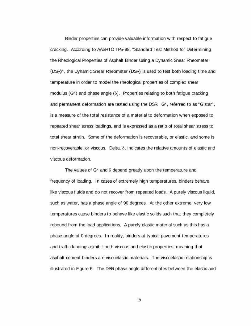
Binder properties can provide valuable information with respect to fatigue
cracking. According to AASHTO TP5-98, “Standard Test Method for Determining
the Rheological Properties of Asphalt Binder Using a Dynamic Shear Rheometer
(DSR)”, the Dynamic Shear Rheometer (DSR) is used to test both loading time and
temperature in order to model the rheological properties of complex shear
modulus (G*) and phase angle (δ). Properties relating to both fatigue cracking
and permanent deformation are tested using the DSR. G*, referred to as “G star”,
is a measure of the total resistance of a material to deformation when exposed to
repeated shear stress loadings, and is expressed as a ratio of total shear stress to
total shear strain. Some of the deformation is recoverable, or elastic, and some is
non-recoverable, or viscous. Delta, δ, indicates the relative amounts of elastic and
viscous deformation.
The values of G* and δ depend greatly upon the temperature and
frequency of loading. In cases of extremely high temperatures, binders behave
like viscous fluids and do not recover from repeated loads. A purely viscous liquid,
such as water, has a phase angle of 90 degrees. At the other extreme, very low
temperatures cause binders to behave like elastic solids such that they completely
rebound from the load applications. A purely elastic material such as this has a
phase angle of 0 degrees. In reality, binders at typical pavement temperatures
and traffic loadings exhibit both viscous and elastic properties, meaning that
asphalt cement binders are viscoelastic materials. The viscoelastic relationship is
illustrated in Figure 6. The DSR phase angle differentiates between the elastic and

20
viscous components of the asphalt binder. G* and δ are both required for
adequately describing material behavior (15, 17).
Relative to fatigue cracking, G* and δ are combined in the calculated term
G*sin δ. According to AASHTO MP1-98, “Standard Specification for Performance
Graded Asphalt Binder”, the value of G*sin δ is restricted to a maximum value of
5000 kPa. DSR tests are performed on binders that have been aged in both the
RTFO and the PAV. Low values of both G* and δ are preferable, and therefore an
elastic binder will provide the best resistance to fatigue cracking. A low G* value
means that the binder has a low resistance to deformation, (i.e. it will “give”)
when subjected to repeated loadings. The low δ value means that the binder is
more elastic, and will “rebound” from the repeated loadings.
Again, modeling the properties of only the binder is not sufficient for
characterizing the pavement’s response to fatigue distress. The aggregate/binder
interactions must be considered. This assessment is accomplished through the
use of the Superpave Shear Tester (SST).
The SST is a shear testing device developed at the University of California
at Berkeley. A photo is given in Figure 5 (20). The SST is a closed-loop feedback,
servo-hydraulic system that was developed to determine the susceptibility of a
pavement to permanent deformation (5, 8). The apparatus includes an extremely
rigid reaction frame and a shear table such that precise displacement
measurements can be obtained as shear loads are applied to the test specimen.
Six tests can be performed using the SST. They are the volumetric test, uniaxial
strain test, repeated shear test at constant stress ratio, repeated shear test at

21
constant height, simple shear test at constant height, and frequency sweep test at
constant height. The results of these tests are used along with a set of
mathematical models in order to predict pavement performance. Performance
prediction involves a material property model, an environmental effects model, a
pavement response model, and a pavement distress model.
The volumetric test and uniaxial strain test use confining pressure in order
to analyze permanent deformation and fatigue cracking in the complete analysis.
The simple shear test at constant height and frequency sweep test at constant
height are used to analyze permanent deformation and fatigue cracking in both
the intermediate and complete analyses. Test parameters vary according to the
extent of the analysis. The repeated shear test at constant height is described
fully in AASHTO TP7-94, “Test Method for Determining the Permanent
Deformation and Fatigue Cracking Characteristics of Hot Mix Asphalt (HMA) Using
the Simple Shear Tester (SST) Device”.
Permanent Deformation
Permanent deformation, or rutting, is the accumulation of small
deformations caused by repeated heavy loads. An example of rutting is given in
Figure 7. Years ago, rutting was not a significant problem. The problem has been
exacerbated by the substantial increase in truck tire inflation pressures (21).
Truck tire pressures have been reported as high as 140 psi (22). One type of
rutting is a structural problem, and can be the result of an under-designed
pavement section or a subgrade that has been weakened by moisture (23). The
other type of rutting is a mixture problem, and is the result of accumulated

22
unrecoverable strain in the asphalt layers due to either densification and/or
repeated shear deformations under applied wheel loads. This type of deformation
is caused by consolidation, lateral movement, or both, of the HMA under traffic
(24). In either case, permanent deformation appears as longitudinal depressions
in the wheel paths of the roadway. Rutting is also a safety issue in that water can
collect in the depressions, increasing the potential for hydroplaning and other
associated wet-weather accidents (25).
There have been many attempts to predict the rutting characteristics of a
pavement, and two basic methods exist. The first is to use failure criterion based
on correlations with road tests or actual field performance. The other is to
compute expected rut depths directly by using empirical relationships or
theoretical computations based on the permanent deformation parameters of each
component layer (18). A number of mathematical relationships have been
developed in order to predict rutting based on stress and/or strain information
derived from laboratory tests. Some use creep tests, some use repeated load
tests, and some use both.
Permanent deformation can be modeled by an empirical equation such that
permanent strain increases at a rate that is dependent on the mixture properties.
The rate of accumulation of permanent strain decreases over time and finally
becomes asymptotic to a value that is also dependent on the mixture properties.
This process is called “strain hardening” because the mixture appears to increase
in stiffness over time. If a mix does not exhibit strain-hardening behavior, it may

23
actually have an increasing rate of accumulation of permanent strain and fall
victim to excessive, or “tertiary” damage (26).
Transverse Profiles
The transverse profile of a pavement contains valuable information that
can be used to determine the contribution of each pavement layer to the observed
total measure of rutting (27). By characterizing the entire transverse profile rather
than simply measuring rut depth, the magnitude, as well as the source of the
rutting can be determined. Thus, rehabilitation needs can be more appropriately
assessed. Also, transverse profile measurements provide greater repeatability
than traditional rut depth measurement methods (28), and can therefore be used
in the calibration of permanent deformation prediction models (27). Research
performed in both Europe and the United States has shown significant
mathematical relationships between transverse profile of the failed pavement and
the cause of failure (27, 28, 29).
The basic idea behind using transverse profile measurements to identify
the source of rutting is that compactive deformation can occur in all layers, and is
characterized by the downward vertical movement of the pavement structure.
Alternatively, plastic deformation involves shifting of the upper HMA pavement
layers such that the deformed surface are higher than the original pavement
surface, often referred to as “heave” (18).
The shape and dimensions of the deformations at the pavement surface
may be used to categorize the pavement into on of four possible types, which are
demonstrated in Figures 8 - 11. The first type is rutting due to the subgrade.
24
Subgrade rutting is characterized by an entirely negative area, meaning that in a
comparison of the original and current transverse profiles, the entire current
profile is at a lower elevation than the original profile. Rutting due to heave is
entirely positive, and is due to an increase in subgrade volume due to
environmental conditions. Base and surface rutting are somewhat similar, having
both positive and negative areas. An overall marginally positive are would be
considered surface rutting, and a marginally negative area would be considered
base rutting. Base rutting is characterized by the appearance of depressions, or
negative area in the wheel paths, and uplift, or positive area between the wheel
paths. Surface rutting is similar, having depressions in the wheel paths and uplift
between the wheel paths, but uplift also appears outside the wheel paths (28).
Permanent Deformation in the Pavement Structure
Mechanistic-empirical design methods exist for pavement design with
respect to permanent deformation. As previously stated, the goal of the
mechanistic-empirical procedures is to determine sufficient layer thickness, based
on fundamental properties, in order to limit pavement distresses.
Mechanistic modeling can either apply to rutting in the subgrade layer
(referred to as the subgrade strain model approach), or to the permanent
deformation within each layer of the pavement. The second approach has not
been widely used (30). In cases where the HMA layers are primarily responsible
for rutting, mechanistic-empirical design is uncertain. The transfer functions that
relate pavement responses to pavement performance are weak because HMA
rutting is not fully understood. Mechanistic-empirical design addresses only the

25
rutting of the entire pavement structure, not the type of rutting that occurs due to
shear failure in HMA surface layers.
Thickness does not necessarily help to prevent rutting near the surface of
the HMA. Therefore material selection and laboratory tests such as repeated
loading and/or creep can help to assess or rank mixes according to their rutting
potential (19). Most methods for measuring permanent deformation employ a
repeated load test, which is similar to a resilient modulus test.
Many prediction models exist for the purpose of predicting accumulated
permanent strain. Rutting is predicted as the accumulation of permanent strain in
the pavement layers under repeated loading. Laboratory tests provide a measure
of the accumulated permanent strain, and mathematical models relate the
measured value to an anticipated level of rutting throughout the design life of the
pavement. Barksdale developed a permanent deformation test procedure in 1972
that involved a repeated triaxial test on a range of granular materials. The
procedure utilized a hyperbolic relation for static stress-strain to model permanent
deformation behavior based on nonlinear elastic layer theory. The model was
used to predict rut depth based on the predicted permanent strain for various
pavement layers given a number of load repetitions, such that the sum of the
permanent strain for the layers was equal to the total rut depth. Barksdale then
defined the rut index as “the sum of the plastic strain in the center of the top and
bottom half of the (granular) base multiplied by 10,000” (31).
Ohio State University developed a permanent strain accumulation
prediction model that includes experimental constants to characterize the material

26
and the state of stress conditions. The proposed permanent strain accumulation
relation is given in Equation 2:
εp / N = ANm Equation 2
where εp is the plastic strain at N number of cycles, N is the number of repeated
load applications, A is an experimental constant depending on material and state
of stress conditions, and m is an experimental constant depending on material
type. Obviously this relationship is only valid for appropriate determinations of the
constants A and m. Extensive research was done relative to the determination of
these constants. Log transformations of the data were useful in calibrating the
model based on field performance (19).
A similar model was developed during the NCHRP 1-10B study (32). The
investigation found that the rate of rutting could be related to surface deflection
and to vertical stress on the surface directly beneath the HMA. A series of
equations were developed based on pavement thickness.
Model calibration is a critical part of mechanistic-empirical modeling. Road
test data has been used in numerous cases to validate mathematical models. In a
1993 study (33), rutting rate analysis was performed on AASHO Road Test flexible
pavements. The results indicated that pavement rutting trends could be
reasonably correlated to the estimated subgrade stress ratio, which is a ratio of
the deviator stress to the unconfined strength of the subgrade.
The Asphalt Institute mechanistic-empirical model has been used
extensively in pavement design as a way to ascertain permanent deformation
characteristics. This model assumes that rutting takes place in the subgrade, and

27
that rutting in the other pavement layers is negligible. This model is given in
Equation 3:
Np = 1.365 * 10-9 * εc-4.477 Equation 3
such that Np is the number of load repetitions to failure due to permanent
deformation based on the vertical compressive strain at the subgrade surface, εc.
A permanent deformation damage ratio is calculated based on an arbitrary failure
criteria. As long as proper compaction of the pavement layers is obtained and the
HMA mixture is properly designed, the use of Equation 3 should not result in more
than 13 mm (0.5 in) of rut depth for the design traffic (18).
A 1998 study (30) compared the AI model with field rutting performance
and found that the AI damage ratio is not a good predictor of rut depth. This is
likely due to the fact that the AI model presumes that the pavement layers above
the subgrade do not contribute much to rutting, which in effect, excludes the
upper pavement layers from the analysis. Field-measured rut depths include
rutting from all sources. The report also stated that because the AI model does
not indicate rutting behavior over time, it cannot account for changes in the rate
of deformation typically experienced by a pavement. A model similar to the AI
model was developed by Shell. This model performs about as well as the AI
model, but produces lower damage estimates. Like the AI model, it neglects
upper pavement contributions to rutting, and cannot model a rate of deformation.
Therefore, neither model is a good predictor of rut depth.
Due to the deficiencies of the AI and Shell models, a new model was
developed, based on the assumption that the relationship between plastic and

28
elastic strains is linear for all pavement layers. It also assumes that this
relationship is nonlinearly related to the number of load repetitions, thereby
allowing for a changing rate of deformation. When the model was calibrated, it
reasonably correlated with field rutting data (30).
Permanent Deformation in the Asphalt Layers
Permanent deformation in the asphalt layers is typically due to either
compactive deformation or plastic deformation. Compactive deformation, or
mixture densification, is a localized, one-dimensional vertical deformation in the
HMA layers. Plastic deformation is due to a lack of resistance to shear failure.
This type of failure occurs along the shear plane of the surface layer such that the
material in the wheel path is displaced laterally from its original location. In other
words, this type of rutting occurs when the shear strength of the asphalt mat is
not great enough to withstand the load of vehicles traversing it. In general, this
type of failure occurs in the top 75-100 mm (3-4 in) of the HMA (34). The shear
deformation in this region is much more significant than rutting due to volume
change (densification). In fact, volume loss in the top 75-100 mm (3-4 in) of the
HMA can account for about 1-2 mm (0.04-0.08 in) of the rut at most, and
therefore the majority of most rutting is due to shear failure (35). Evaluations
relating to shear failure should be made using samples that best represent the
upper portion of the HMA layer, both in terms of aggregate structure and level of
compaction. For these reasons, the top two layers of HMA can be the most
critical. A properly designed HMA mixture possessing a strong interlocking

29
aggregate structure combined with a binder of adequate stiffness can significantly
reduce a pavement’s susceptibility to this type of rutting failure (8).
Many factors can affect the shear resistance of a mix. Experience shows
that stiff binders with large aggregates typically are more resistant to rutting than
mixes containing finer aggregates and higher binder content (13). Natural
(rounded) sands increase a mixture’s susceptibility to rutting (36). The rounded
particles can function as ball-bearings, reducing the stability of the mix. Coarse
aggregates provide the skeleton of the mixture, and since larger aggregate
particles are considered to be stronger than fine aggregate particles, a coarse-
graded aggregate blend should provide a rut-resistant mix structure. Binder
content is also important. Binder film thickness should be adequate for coating
the aggregate and providing cohesion, but too much binder can actually have a
lubricating effect, creating an unstable mix (36).
Air voids play a significant role in a mixture’s resistance to shear failure.
HMA mixes are typically most stable at some air void content between 3 and 7
percent. In-place air void contents below about 3 percent have been shown to
greatly increase the probability of premature rutting (34, 36). High air voids
(above 7 percent) can also increase the likelihood of rutting. At high air void
contents, poorly compacted mixes can experience considerable shear flow. To
avoid this phenomenon, the HMA should be compacted to a void content well
above 3.0 percent, (in the range of approximately 5 to 7 percent) using an
adequately high compactive effort so that the voids remain above 3.0 percent
even under expected traffic. In general, rutting resistance can be increased
30
through the use of angular aggregates, appropriate binder contents, and by
keeping the air void content at an appropriate level.
Permanent Deformation Tests
Marshall and Hveem mixture design methods sought to address this type
of distress through volumetric relationships and a measurement of stability.
However, these stability tests did not always adequately predict the rutting
resistance of the mix (35, 37, 38, 39).
Superpave Shear Tester
Superpave recommends the use of the SST for the assessment of mixtures
with respect to shear resistance. In fact, all six tests mentioned by Superpave for
use in the SST relate to rutting. During each of these tests, axial and shear loads
and deformations are measured and recorded. G*/sin δ is again the parameter
used to evaluate a mixture’s resistance to shear failure. A well-compacted mix
with a good aggregate structure will develop a high axial stress at small shear
strain levels. Poor mixes can generate similar levels of axial stresses but require
much higher shear strains to do so. The rate of permanent deformation is related
directly to the magnitude of the shear strain (20).
In a complete Superpave analysis, the volumetric test and uniaxial strain
test use confining pressure in order to analyze permanent deformation
characteristics. Repeated shear at constant stress ratio (RSCSR) is used as a
screening test for tertiary rutting, which is severe plastic flow of the mix which
occurs when the air void content becomes very low – less than 2 or 3 percent.

31
The simple shear test at constant height (SSCH) and frequency sweep test
at constant height (FSCH) are used to analyze permanent deformation in both the
intermediate and complete levels of analysis. The FSCH test is the only SST
method that uses dynamic loading (11). The resulting G* and δ values from the
FSCH can be converted to complex creep compliances. The FSCH characterizes
the viscoelastic behavior of asphalt/aggregate mixtures, similar to the DSR test
that is performed on binders. The results of these tests are intended for use with
the material property, environmental effects, pavement response, and
environmental effects models. The phase angle, δ, is highly temperature and
frequency dependent. At high frequencies and low temperatures, δ is affected
primarily by the asphalt binder. At low frequencies and high temperatures, it is
affected more by the aggregate structure (40).
The repeated shear test at constant height (RSCH) is not required by
Superpave, but can be used to estimate rut depths. It can also aid in determining
the optimum binder content of a mixture. This test method is described fully in
AASHTO TP7-94, “Test Method for Determining the Permanent Deformation and
Fatigue Cracking Characteristics of Hot Mix Asphalt (HMA) Using the Simple Shear
Tester (SST) Device”. The RSCH method has recently gained popularity as a
measure of shear resistance of HMA mixtures (41). The main advantage to this
method is that it obtains properties in useful engineering units, which can be used
in performance prediction models (20). It also has proven to be a better predictor
of permanent deformation characteristics than traditional devices, such as the
Hveem stabilometer (35). However, direct measurements of G* have shown that

32
it may be nonlinear with respect to frequency, temperature, and strain level. Its
greatest variability occurs at low temperatures and high frequencies (42).
Dynamic creep testing has also been used to evaluate mixes with respect
to cumulative residual strain as a function of time (43). However, it has been
suggested that repeated loads, rather than creep loading, should be used to
determine the susceptibility of a mix to rutting (20).
The SST is a valuable tool for analyzing permanent strain parameters of an
HMA mixture. However, it is relatively expensive and not readily available to all
mix designers. Several other methods have been developed as a means for a
relatively quick and less expensive determination of rutting susceptibility.
Superpave Binder Specification
The Superpave binder specification addresses shear resistance through
DSR testing. The complex shear modulus, G*, and phase angle, δ, are the two
DSR values used in AASHTO MP1-98 used to indicate rutting resistance.
Requirements are placed on the calculated value of G*/sin δ at the test
temperature both before and after aging in the RTFO. G*/sin δ must be a
minimum of 1.0 kPa before aging, and a minimum of 2.20 kPa after aging in the
RTFO. In order to minimize rutting, high G* values and low δ values are helpful,
meaning that stiff, elastic binders help to address problems associated with
permanent deformation (37).
Gyratory Load-Cell-Plate-Assembly
Another of these methods involves a device known as the Gyratory Load-
Cell-Plate-Assembly (GLPA). This device was developed to measure the shear

33
resistance of HMA during compaction. The device is inserted on top of the
mixture inside the compaction mold during the typical compaction procedure. The
GLPA provides a continuous measurement of the resistance to shear under the
gyratory loading at a fixed angle, providing immediate results (12). The greatest
advantage of this device is that it can be used with the gyratory compactor during
compaction providing quick results. This method appears to have the potential to
provide information regarding the shear resistance and stability of HMA, although
more research is needed to relate laboratory results to field performance.
Gyratory Ratio
Another method is used to determine shear resistance is known as the
gyratory ratio. The gyratory ratio is the ratio of the number of gyrations required
to achieve 2 percent voids to the number of gyrations required to achieve 5
percent voids. The underlying assumption is that a stable mix will have similar or
increased shear strength at 2 percent voids as compared to 5 percent voids. In
fact, if a gyratory ratio is less than 4, then the mix might be expected to be
unstable (44). Because it requires no equipment in addition to the SGC, this idea
could prove be a useful screening tool for HMA mixtures.
Gyratory Testing Machine
The Corps of Engineers (COE) Gyratory Testing Machine (GTM) is a
combination compaction and plane strain shear testing machine that applies
stresses simulating pavement conditions. Shear susceptibility can be assessed
using the static shear strength (Sg), gyratory stability index (SGI), gyratory
elastoplastic index (GEPI), and refusal air voids level. The SGI is the ratio of the
34
maximum angle that occurs at the end of the test to the minimum intermediate
angle. It measures the shear susceptibility at the refusal density. The GEPI is the
ratio of the minimum intermediate angle to the initial machine angle set by the
operator (37).
Proof Tests
Proof tests have emerged as one of the most acceptable options available
to most mix designers as a method for determining rutting susceptibility. Wheel
tracking tests are the most popular type of proof test. In these tests, asphalt
mixture samples are subjected to moving wheel loads in order to determine if they
are susceptible to rutting or a related failure mode, stripping. These types of tests
attempt to recreate situations found in the field by performing accelerated tests to
estimate actual field performance. Wheel-tracking tests will be discussed in full
detail in subsequent sections of this paper.
Moisture Susceptibility
Moisture susceptibility, or stripping, is defined as the weakening or
eventual loss of the adhesive bond mainly due to the presence of moisture and/or
moisture vapor between the aggregate surface and the asphalt cement in an HMA
pavement or mixture (1). Often, water is trapped at the bottom of the asphalt
layer, so the failure begins at the bottom of the asphalt and gradually progresses
upward to the surface (45). As the asphalt binder is separated from the
aggregate particles, the aggregate is no longer held in place. It begins to shift
and condense, causing a depression in the surface of the pavement, and often
appears as rutting. Stripping in the field can be differentiated from rutting by an

35
experienced pavement engineer. Traffic-induced stripping appears as rutting
where the rise and flow from shear failure is centered on the wheel path but has
an irregular width. It may also appear as a localized shear failure that is centered
on the wheel path (46). In extreme cases of stripping, bare aggregate particles
are actually visible at the surface. Ultimately raveling occurs, meaning that the
loose particles are forced from the surface by the action of traffic loadings.
Some stripping relates to a physio-chemical incompatibility of the
asphalt/aggregate system. However all asphalt mixes may fail as a result of the
cyclic hydraulic stress physically scouring the asphalt binder from the aggregate.
The presence of water, high stress, and high temperatures promote stripping.
Some moisture is always present in HMA, and in wet seasons the pavements may
become saturated. Cyclic pore water pressure is generated by traffic. Neither
saturation nor traffic can be prevented, and therefore stripping is a possible
outcome. This type of stripping is a mechanical failure of the asphalt (47).
Stripping due to physio-chemical incompatibilities may be associated with
two mechanisms – loss of adhesion and loss of cohesion. Loss is adhesion is due
to water getting between the asphalt and aggregate, thus stripping away the
asphalt film. Loss of cohesion is due to a softening of the asphalt cement in the
presence of water. This weakens the bond between the asphalt cement and the
aggregate. Water is then able to get between the asphalt and aggregate because
the aggregate has a greater attraction to water than to asphalt cement. These
two mechanisms are interrelated such that moisture damage may be the result of
a combination of both cohesion and adhesion losses (48).

36
Moisture damage due to mechanical failures may be a function of several
factors such as the characteristics of the asphalt mixture, the environment, and
construction practices. Asphalt concrete factors include the nature of the
aggregate, the nature of the asphalt cement, and the type of mixture. Clean
aggregates with a rough surface texture and low surface moisture combined with
asphalt binders of high viscosity are more resistant to moisture damage.
Environmental factors include climate and traffic loadings. Extreme weather
conditions, especially freeze-thaw action, combined with heavy traffic loadings
tend to cause the most moisture damage. Compaction level and weather
conditions during construction also affect resistance to moisture damage. In-place
air void content is generally thought to be the most important construction factor
(48).
Stripping was studied as early as the 1950s, but research efforts began to
intensify during the mid-1970s (49). In the 1970s, several developments occurred
that could have inadvertently aided in the production of more moisture damage
susceptible HMA mixtures. The 1972 Clean Air Act resulted in baghouse fines
being collected and to some extent added back to the mix. These fine particles,
which can negatively affect moisture susceptibility, were previously not a part of
the mix. Also, vibratory rollers became more common, and the use of pneumatic
tire rollers for intermediate compaction was mostly phased out. These rollers
were believed to help “seal” the surface of the HMA, preventing the entrance of
moisture into the mat, and thus reducing the potential for stripping. The use of
siliceous aggregates, which are somewhat prone to stripping, were promoted for

37
their advantage of increased skid resistance. Siliceous aggregate have been
classified as “hydrophilic” and tend to strip more readily than limestone
aggregates, which are classified as “hydrophobic” (50). Thus, the use of siliceous
aggregates to achieve skid resistance may have compromised HMA aggregate
quality relative to stripping. Finally, film thicknesses decreased. Film thicknesses
that are too large have a tendency to lubricate the aggregate, thereby promoting
permanent deformation. The decrease in film thickness was used as a way to
mitigate the rutting susceptibility of HMA mixes (47).
If an HMA mix is determined to be stripping susceptible, antistripping
additives may by added to the mix. The two main types of antistripping additives
are chemical liquid agents and hydrated lime (49). Chemical additives decrease
the surface tension of the asphalt and can also help to form a chemical bond
between the asphalt and silica component of the aggregate, which is known to be
prone to stripping (48). Hydrated lime is added either to damp aggregate or as a
slurry. It is suggested that hydrated lime reacts strongly with the carboxylic acids
of the asphalt, so that fewer are adsorbed by the aggregate surfaces, creating a
stronger asphalt-aggregate bond (51). One survey indicated that treating
aggregate with hydrated lime is the most effective additive for the prevention of
moisture damage (48).
Several fine aggregate characteristics can promote moisture susceptibility.
A coating of dust or clay particles may prevent adequate adhesions between the
asphalt binder and coarse aggregate particles. Also, smooth aggregate particles
do not adhere to asphalt cement as well as aggregate particles with angular or
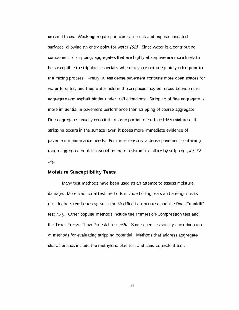
38
crushed faces. Weak aggregate particles can break and expose uncoated
surfaces, allowing an entry point for water (52). Since water is a contributing
component of stripping, aggregates that are highly absorptive are more likely to
be susceptible to stripping, especially when they are not adequately dried prior to
the mixing process. Finally, a less dense pavement contains more open spaces for
water to enter, and thus water held in these spaces may be forced between the
aggregate and asphalt binder under traffic loadings. Stripping of fine aggregate is
more influential in pavement performance than stripping of coarse aggregate.
Fine aggregates usually constitute a large portion of surface HMA mixtures. If
stripping occurs in the surface layer, it poses more immediate evidence of
pavement maintenance needs. For these reasons, a dense pavement containing
rough aggregate particles would be more resistant to failure by stripping (49, 52,
53).
Moisture Susceptibility Tests
Many test methods have been used as an attempt to assess moisture
damage. More traditional test methods include boiling tests and strength tests
(i.e., indirect tensile tests), such the Modified Lottman test and the Root-Tunnicliff
test (54). Other popular methods include the Immersion-Compression test and
the Texas Freeze-Thaw Pedestal test (55). Some agencies specify a combination
of methods for evaluating stripping potential. Methods that address aggregate
characteristics include the methylene blue test and sand equivalent test.
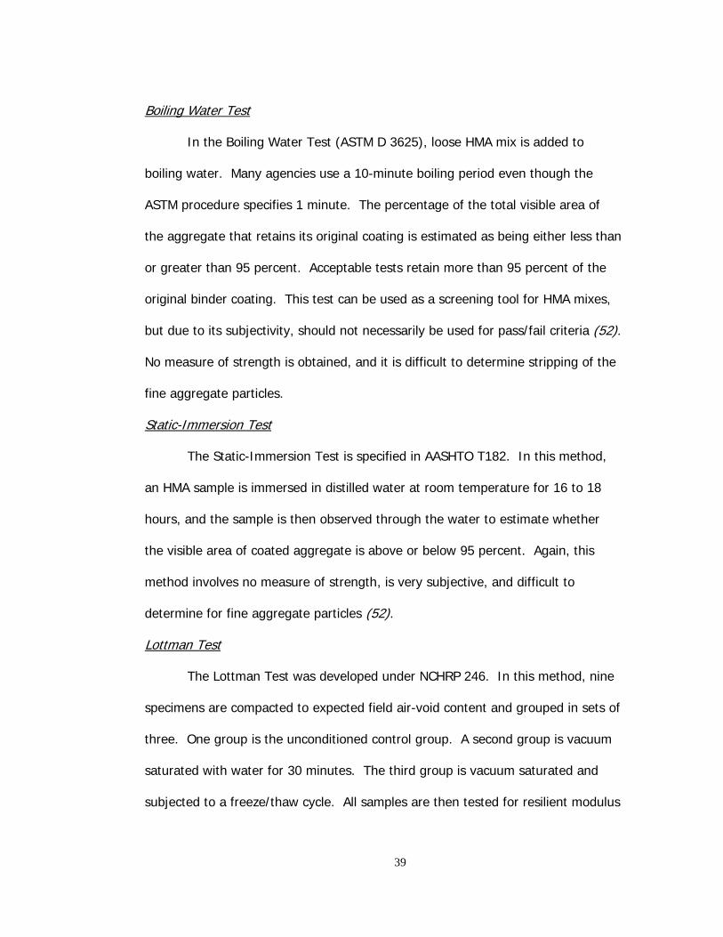
39
Boiling Water Test
In the Boiling Water Test (ASTM D 3625), loose HMA mix is added to
boiling water. Many agencies use a 10-minute boiling period even though the
ASTM procedure specifies 1 minute. The percentage of the total visible area of
the aggregate that retains its original coating is estimated as being either less than
or greater than 95 percent. Acceptable tests retain more than 95 percent of the
original binder coating. This test can be used as a screening tool for HMA mixes,
but due to its subjectivity, should not necessarily be used for pass/fail criteria (52).
No measure of strength is obtained, and it is difficult to determine stripping of the
fine aggregate particles.
Static-Immersion Test
The Static-Immersion Test is specified in AASHTO T182. In this method,
an HMA sample is immersed in distilled water at room temperature for 16 to 18
hours, and the sample is then observed through the water to estimate whether
the visible area of coated aggregate is above or below 95 percent. Again, this
method involves no measure of strength, is very subjective, and difficult to
determine for fine aggregate particles (52).
Lottman Test
The Lottman Test was developed under NCHRP 246. In this method, nine
specimens are compacted to expected field air-void content and grouped in sets of
three. One group is the unconditioned control group. A second group is vacuum
saturated with water for 30 minutes. The third group is vacuum saturated and
subjected to a freeze/thaw cycle. All samples are then tested for resilient modulus
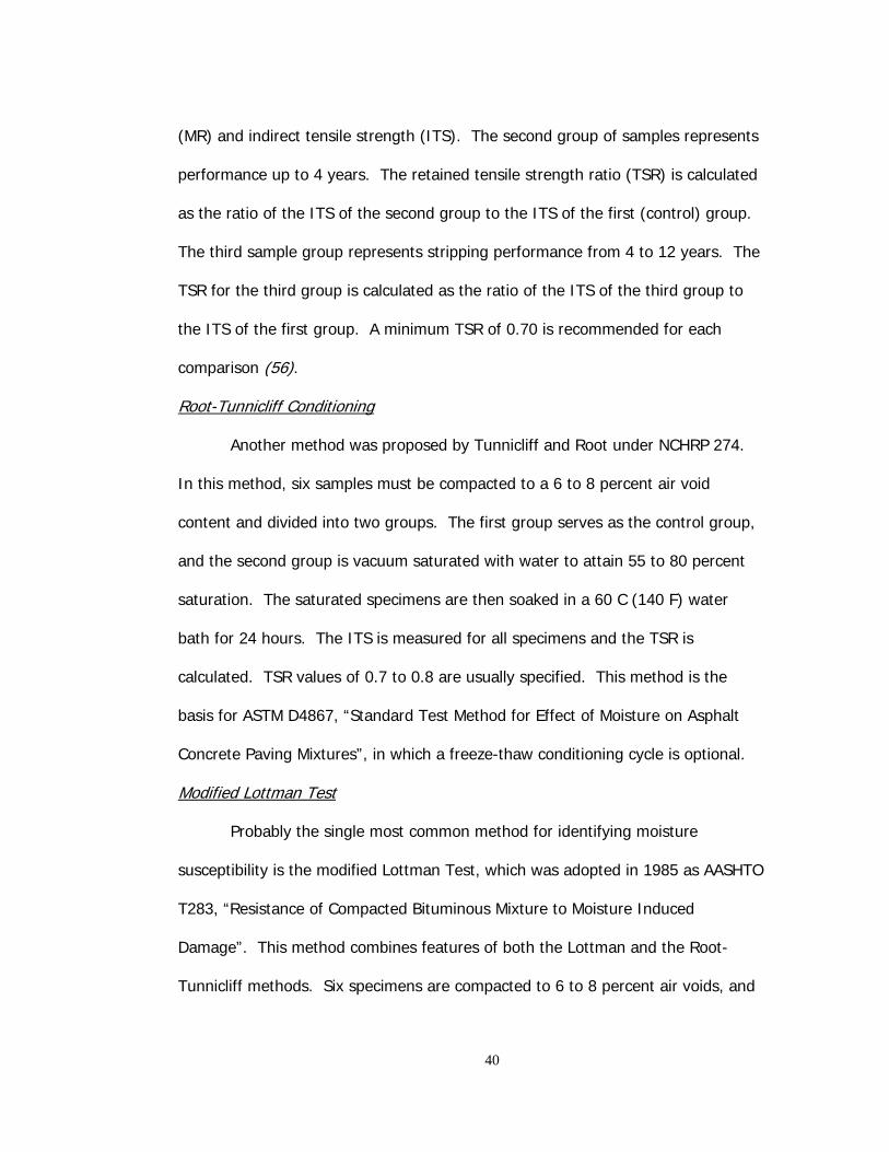
40
(MR) and indirect tensile strength (ITS). The second group of samples represents
performance up to 4 years. The retained tensile strength ratio (TSR) is calculated
as the ratio of the ITS of the second group to the ITS of the first (control) group.
The third sample group represents stripping performance from 4 to 12 years. The
TSR for the third group is calculated as the ratio of the ITS of the third group to
the ITS of the first group. A minimum TSR of 0.70 is recommended for each
comparison (56).
Root-Tunnicliff Conditioning
Another method was proposed by Tunnicliff and Root under NCHRP 274.
In this method, six samples must be compacted to a 6 to 8 percent air void
content and divided into two groups. The first group serves as the control group,
and the second group is vacuum saturated with water to attain 55 to 80 percent
saturation. The saturated specimens are then soaked in a 60 C (140 F) water
bath for 24 hours. The ITS is measured for all specimens and the TSR is
calculated. TSR values of 0.7 to 0.8 are usually specified. This method is the
basis for ASTM D4867, “Standard Test Method for Effect of Moisture on Asphalt
Concrete Paving Mixtures”, in which a freeze-thaw conditioning cycle is optional.
Modified Lottman Test
Probably the single most common method for identifying moisture
susceptibility is the modified Lottman Test, which was adopted in 1985 as AASHTO
T283, “Resistance of Compacted Bituminous Mixture to Moisture Induced
Damage”. This method combines features of both the Lottman and the Root-
Tunnicliff methods. Six specimens are compacted to 6 to 8 percent air voids, and

41
separated into two groups. The first group serves as the control group. The
second group is subjected to vacuum saturation as well as a freeze/thaw cycle.
Conditioned samples are to reach 55 to 80 percent saturation. The TSR is
determined as the ratio of the ITS of the conditioned group to the ITS of the
control group. Specified minimum TSR values range from 0.70 to 0.85 (52, 57,
58). AASHTO T283 has gained prominence in recent years due to the fact that it
was the method chosen by SHRP researchers as the test for moisture damage in
Superpave mixture design, with a minimum TSR of 0.80 (57). This method has
not, however, been calibrated for used with mix samples produced using the SGC
(59).
Most highway agencies use a wet-to-dry cutoff ratio for moisture damage
of 0.7 for resilient modulus testing or 0.75 for indirect tensile strength. In 1990,
Lottman recommended new ratios of 0.80 and 0.85 in order to control moisture
susceptibility for both fatigue cracking and for wheel path rutting (60). Both
resilient modulus cut-of ratio AND tensile strength ratio are to be used for fatigue
cracking tests, while the MR ratio is necessary to control wheel path rutting
distress. Both are needed to control both distresses. Most state agencies use
indirect tension tests, which are used to derive resilient modulus ratios (MRR) and
tensile splitting strength ratios (TSR).
Immersion-Compression Test
The Immersion-Compression Test is detailed in AASHTO T165. In this
method, six specimens are compacted with a double plunger at a pressure of 20.7
MPa (3,000 psi) for two minutes to approximate seven percent air voids. The

42
specimens are grouped in two sets of three. The first set is the control group.
The second group is subjected to submersion in water at 49 C (120 F) for four
days or at 60 C (140 F) for one day. All specimens are tested for unconfined
compressive strength. The retained compressive strength is determined, and is
usually required to be at least 70 percent. This test has been reported to lack
precision (52).
Texas Freeze-Thaw Pedestal Test
The Texas Freeze-Thaw Pedestal test involves placing compacted and
cured specimens on a pedestal in a water bottle. Samples are subjected to freeze-
thaw cycles until cracking appears. This test is very subjective, requiring visual
examination. There is only a fair correlation between field and lab results, and
only cohesion is measured (48).
Net Adsorption Test
A Net Adsorption Test (NAT) was developed under SHRP A-003B and
completed by the National Center for Asphalt Technology. It is a preliminary
screening test to be used for matching mineral aggregates and asphalt cement.
The method is based on principles of adsorption and desorption (61). A solution
of asphalt cement and toluene is combined in a reaction column with the
aggregate sample. Once the temperature has been stabilized, 4 ml of solution is
removed and the absorbance is determined with a spectrophotometer. Next, 40
grams of aggregate passing the 4.75-mm (#4) sieve is added to the column, and
the solution circulated for 6.5 hours. The absorbance is again determined, and

43
the difference in the two readings is used to determine the amount of asphalt that
has been removed from the solution by adsorption.
Environmental Conditioning System
The Environmental Conditioning System (ECS) was developed during SHRP
Project A-003A (52). In this method, HMA samples are compacted to 7.5 ± 0.5
percent air voids, and then placed in a latex membrane and secured with silicone.
Samples are required to be 102 ± 2 mm in both diameter and height. Air
permeability and dry resilient modules (MR) of the specimen are measured soon
after the sample is placed in the ECS loading frame. Next the specimen is vacuum
saturated and the water permeability determined. The sample is then subjected
to a six hour “hot cycle” while subjected to a cyclic loading. Then the specimen is
cooled to approximately room temperature. Two repetitions of the
heating/loading and cooling cycles are applied, and in some regions, a six-hour
freeze cycle may be inserted into the test pattern. The hot-cold cycling represents
actual field exposure, and the repeated loading simulates traffic.
At the end of each cycle, the conditioned MR is recorded and a ratio to the
unconditioned MR is calculated. If the ratio is less than 0.70, then the sample is
considered to be moisture susceptible (62). At the completion of the test, the
indirect tensile strength of the sample can be measured. Samples can also broken
apart in order to visually determine the severity of stripping.
ECS testing is intended to use resilient modulus testing, which is better
than indirect tensile strength (ITS). MR testing is preferred because it is
nondestructive, so the conditioned and unconditioned MRs can be tested on the

44
same specimen (62). ITS, on the other hand, are destructive tests, and some
material variability can be present in the multiple specimens used for the testing.
The ECS is a less severe test than AASHTO T283 (63). Overall, it appears to be a
versatile system, but it is expensive (52).
Ultrasonic Method
The ultrasonic moisture accelerated conditioning process is a new method
being researched in Nevada for the purpose of quantifying the moisture sensitivity
of an asphalt mixture (64). Samples are placed in a water bath that is maintained
at a constant temperature of 60 C (140 F). A repeated cycle of compression then
cavitation accelerates the detachment and displacement of the asphalt binder from
the aggregate surface. Cavitation is the formulation and then collapse of
microscopic vacuum bubbles created by the pressure waves within the water bath.
The results of the ultrasonic test for stripping are similar to that obtained by
AASHTO T283 after 18 cycles of freeze-thaw conditioning.
Methylene Blue Test
The type of material passing the 0.075-mm (#200) sieve has a significant
impact on the susceptibility of an HMA pavement to moisture damage (65).
Plastic fines can be detrimental to the stripping performance of HMA mixes (66).
Thus, special aggregate tests can be used as a method of detection for moisture
susceptibility of an HMA mix. Methylene blue and sand equivalent tests are
required in France, and can be used to predict moisture susceptibility. These tests
target the characteristics of the fine material passing the 0.075-mm (#200) sieve.

45
In the methylene blue test, 1 g of material passing the 0.075-mm (#200)
sieve is mixed with 30 g of distilled water. A solution of methylene blue is added
in increments, and stirred continuously. After one minute, a small drop of the
aggregate solution is placed on filter paper. If a halo does not form around the
drop, then another increment of methylene blue is added. The process is
repeated until a halo around the drop is evident. This test identifies the presence
of smectite, a poor quality clay, which is an undesirable component in fine
aggregate. The test also identifies a level of surface activity of the aggregate.
The lesser the concentration of methylene blue causing the halo to appear, the
more active the aggregate surface. Active fines are less susceptible to moisture
damage than inactive fines. Thus, low methylene blue values (MBVs) are
expected to correlate with increased resistance to moisture damage (67).
Sand Equivalent Test
The sand equivalent test is performed according to AASHTO T176, and
determines how “clean” the material is that passes the 4.75-mm (#4) sieve. In
this test, an aggregate is placed in a graduated cylinder with flocculating solution
and agitated. This action loosens clay particles from the surfaces of larger
aggregate. The non-clay material is allowed to settle, and the heights of both the
suspended clay and the sand sediment are measured. The sand equivalent is a
ratio of the height of sand to the height of clay. A higher ratio indicates cleaner
material. In the United States, required values for this test method are in the
range of 40 to 50. Higher values are required in Europe (67).

46
Dust Coating Measurement
Because dust coating on aggregates can prevent adequate bonding
between the aggregate and asphalt cement binder, dust coatings on coarse
aggregates can be detrimental to a pavement’s performance with respect to
moisture damage. In one study, the dust coating was measured by taking a
sample of material retained on the 4.75-mm (#4) sieve by dry sieving. Next, the
material was washed over a 4.75-mm (#4) sieve and dried. The difference in
mass of material before and after washing was defined as the dust coating,
expressed as a percentage. If the dust coating exceeds 3 percent, the aggregate
may be susceptible to moisture damage (67).
Rigden Voids Index
Stiffness is known to affect both fatigue and thermal cracking
characteristics of a pavement, but it can also affect moisture susceptibility. As
dust, or aggregate passing the 0.075-mm (#200) sieve, is combined with asphalt
binder, the mixture stiffens. As the binder stiffness increases, the resistance to
moisture damage should also increase. The Rigden voids index test can be used as
a measure of stiffening, and is an estimation of the volume of free asphalt cement
binder in a dust-asphalt mixture, expressed as a percentage of total mixture
volume. Higher levels of free asphalt binder are desirable (67). Minimum values
of 40 and 50 percent have been recommended (65, 68, 69).
Stiffening power can also be measured as the difference in the ring and
ball softening point temperatures of the neat asphalt binder and the asphalt binder
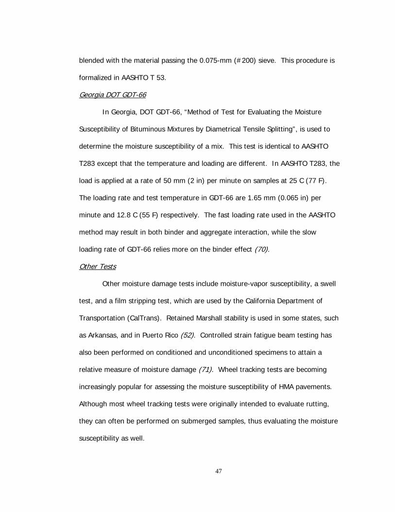
47
blended with the material passing the 0.075-mm (#200) sieve. This procedure is
formalized in AASHTO T 53.
Georgia DOT GDT-66
In Georgia, DOT GDT-66, “Method of Test for Evaluating the Moisture
Susceptibility of Bituminous Mixtures by Diametrical Tensile Splitting”, is used to
determine the moisture susceptibility of a mix. This test is identical to AASHTO
T283 except that the temperature and loading are different. In AASHTO T283, the
load is applied at a rate of 50 mm (2 in) per minute on samples at 25 C (77 F).
The loading rate and test temperature in GDT-66 are 1.65 mm (0.065 in) per
minute and 12.8 C (55 F) respectively. The fast loading rate used in the AASHTO
method may result in both binder and aggregate interaction, while the slow
loading rate of GDT-66 relies more on the binder effect (70).
Other Tests
Other moisture damage tests include moisture-vapor susceptibility, a swell
test, and a film stripping test, which are used by the California Department of
Transportation (CalTrans). Retained Marshall stability is used in some states, such
as Arkansas, and in Puerto Rico (52). Controlled strain fatigue beam testing has
also been performed on conditioned and unconditioned specimens to attain a
relative measure of moisture damage (71). Wheel tracking tests are becoming
increasingly popular for assessing the moisture susceptibility of HMA pavements.
Although most wheel tracking tests were originally intended to evaluate rutting,
they can often be performed on submerged samples, thus evaluating the moisture
susceptibility as well.

48
WHEEL TRACKING TESTS
Due to the relatively great expense and variable testing results, Superpave
performance testing equipment has not been overwhelmingly accepted by the
HMA industry. Wheel tracking tests are quickly becoming the most common type
of laboratory equipment used for the determination of rutting susceptibility (24).
With respect to moisture damage, many test methods have been used, but none
have been superior in determining stripping susceptibility. Wheel tracking could
be the answer to this question as well. Wheel track testing has even been used to
assess fatigue response of HMA mixes (72, 73).
The loaded wheel test (LWT) offers an excellent device for quantitatively
comparing the relative rutting susceptibility of one HMA mix with another. The
two main advantages of the LWT are that 1) the stress state applied to the sample
is somewhat similar to that which occurs in the field, and 2) it is relatively
inexpensive and easy to operate. The disadvantage is that no fundamental
property, such as resilient modulus, is obtained from this test for use in
mechanistic-empirical design models (74).
All LWTs operate under the same general premise – a loaded moving
wheel travels along the sample lengthwise while applying a load to the sample in
order to simulate rutting. Depressions, or ruts, are created in the sample. The
magnitudes of the rut depths are measured and recorded. LWT data can be used
to rank the performance of a variety of mixes, or pass/fail criteria can be applied
for mixture acceptance. The parameters of air voids and test temperature are
usually specified, while other parameters, such as sample type, pressure, load,

49
and length of test can be variable and must be determined based on experience or
manufacturer recommendations.
The Europeans have taken the lead in developing accelerated pavement
testing devices (7). In September of 1990, a group of individuals representing the
American Association of State Highway and Transportation Officials (AASHTO),
Federal Highway Administration (FHWA), National Asphalt Pavement Association
(NAPA), Strategic Highway Research Program (SHRP), Asphalt Institute (AI), and
the Transportation Research Board (TRB) participated in a two-week tour of six
European countries to survey the types of performance-related testing equipment
being used in Europe. Since that time, there have been a number of studies
conducted to develop information on the various types of LWTs. The states of
Colorado, Texas, and Georgia, among others, have been leaders in promoting the
use of LWTs for predicting both rutting and moisture susceptibility. Table 1
provides a comparison of several types of wheel tracking devices.
Hamburg Wheel Tracking Device
The Hamburg Wheel-Tracking Device (HWTD), shown in Figure 12, was
developed in the 1970s by Esso A.G. of Hamburg, Germany (75). It is based on a
similar British device using a rubber tire. The HWTD is currently marketed by
Helmut-Wind Incorporated of Hamburg, Germany. It is used as a specification
requirement for some of the most traveled roadways in Germany with regard to
rutting and stripping (76). The HWTD was originally used to measure rutting
susceptibility. The test required 9540 wheel passes at temperatures of 40 C (104
F) and 50 C (122 F). The test was then lengthened to 19,200 passes, and it was
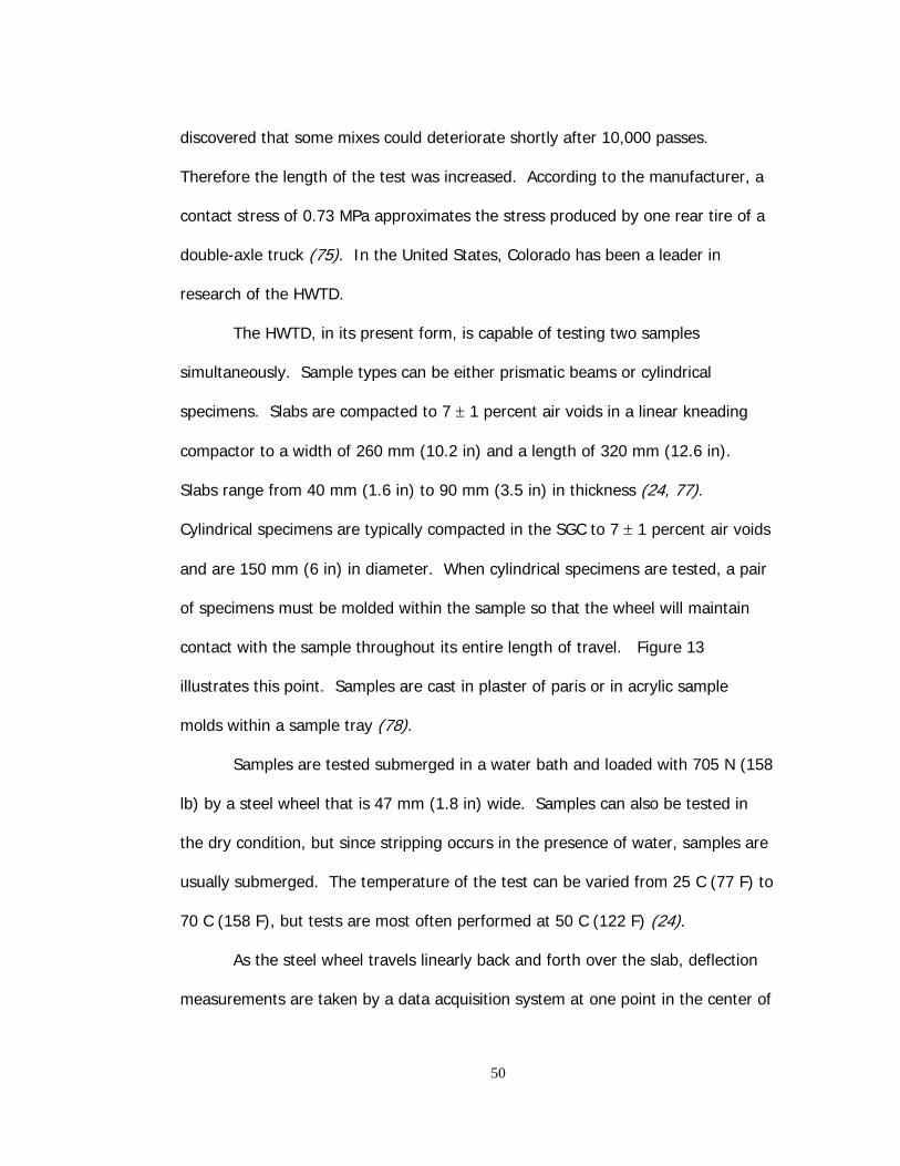
50
discovered that some mixes could deteriorate shortly after 10,000 passes.
Therefore the length of the test was increased. According to the manufacturer, a
contact stress of 0.73 MPa approximates the stress produced by one rear tire of a
double-axle truck (75). In the United States, Colorado has been a leader in
research of the HWTD.
The HWTD, in its present form, is capable of testing two samples
simultaneously. Sample types can be either prismatic beams or cylindrical
specimens. Slabs are compacted to 7 ± 1 percent air voids in a linear kneading
compactor to a width of 260 mm (10.2 in) and a length of 320 mm (12.6 in).
Slabs range from 40 mm (1.6 in) to 90 mm (3.5 in) in thickness (24, 77).
Cylindrical specimens are typically compacted in the SGC to 7 ± 1 percent air voids
and are 150 mm (6 in) in diameter. When cylindrical specimens are tested, a pair
of specimens must be molded within the sample so that the wheel will maintain
contact with the sample throughout its entire length of travel. Figure 13
illustrates this point. Samples are cast in plaster of paris or in acrylic sample
molds within a sample tray (78).
Samples are tested submerged in a water bath and loaded with 705 N (158
lb) by a steel wheel that is 47 mm (1.8 in) wide. Samples can also be tested in
the dry condition, but since stripping occurs in the presence of water, samples are
usually submerged. The temperature of the test can be varied from 25 C (77 F) to
70 C (158 F), but tests are most often performed at 50 C (122 F) (24).
As the steel wheel travels linearly back and forth over the slab, deflection
measurements are taken by a data acquisition system at one point in the center of

51
the specimen. Rut depths are recorded every 100 passes, and are accurate to
0.01 mm (54, 78). A test is complete when a total of 20,000 wheel passes have
been applied or the sample accumulates 20 mm (0.8 in) of rut depth. The wheel
makes 50 passes over each sample per minute. The maximum velocity of the
wheel is 34 cm/sec (1.1 ft/sec) in the center of the sample. At this rate, a HWTD
test takes approximately 6.5 hours (24, 79).
Recorded rut depths are plotted against the number of passes. A typical
data plot is given in Figure 14. A typical sample will experience some initial
consolidation, or post-compaction, then deform at a rate known as the creep
slope, or rutting slope. Results from the HWTD include the rutting slope, stripping
slope, and stripping inflection point. The rutting slope relates to rutting from
plastic flow. It is defined as the inverse of the rate of deformation in the linear
region of the deformation curve, after initial consolidation effects have ended and
before the onset of stripping. In other words, it is the number of passes after the
initial consolidation required to create a 1-mm rut. The stripping slope is the
inverse of the rate of deformation in the linear region of the deformation curve,
after stripping begins and until the end of the test. It is the number of passes
required to create a 1-mm impression from stripping. The stripping slope is
related to the severity of moisture damage. The stripping inflection point is the
number of passes at the intersection of the rutting slope and the stripping slope.
It is the point where rutting begins to be dominated by moisture damage, and is
related to the resistance of the HMA to moisture damage (79).

52
Failure, according to the German specification, is defined as having a rut
depth greater than 4 mm (0.16 in) after 20,000 wheel passes (77). This criteria
was considered to be too harsh for many pavements in the U.S. The state of
Colorado currently uses a maximum rut depth criteria of 10 mm (0.4 mm) (80).
The repeatability of this device is reported to be acceptable (81).
French Rut Tester
The French have developed what is known as the French Rut Tester (FRT).
The FRT, shown in Figure 15, was developed in the 1970s and 1980s at the
Laboratoire Central des Ponts et Chausees (LCPC). It was first developed for a
practical mix design study tool, and is used on an empirical basis during HMA
mixture design in France (78). The test method is detailed in the French Standard
AFNOR Standard 98253, which has been in place since 1991. As of 1993, 72 FRT
devices were in service, 45 of which were in France (36).
The FRT is capable of testing two samples simultaneously within an
environmental chamber that encloses the specimens. Samples are usually
prismatic beams, which are compacted in the LCPC plate compactor. The LCPC
compactor was developed specifically for the purpose of compacting specimens for
the FRT. The LCPC compactor and the FRT are typically sold together as a set.
Slab samples are typically 180 mm (7.1 in) wide, 500 mm (19.7 in) long, and 20 to
100 mm (0.8 to 3.9 in) thick. During testing, a pneumatic tire inflated to 600 kPa
(87 psi) travels back and forth over the sample, applying a load of 5000 N (1124
lb) at a rate of two passes per second. A pair of slabs can be tested in
approximately 9 hours. The tire has a diameter of 415 mm (16 in) and a width of

53
109 mm (4.3 in). The wheel travels at a speed of 1.6 m/s (5.2 ft/s). A 60 C (140
F) testing temperature is recommended for wearing courses, and a 50 C (122 F)
test temperature is recommended for base courses. The device has the capability
of testing at any temperature between 35 C (95 F) and 60 C (140 F) (77, 78, 82,
83, 84).
At the beginning of the FRT test, a “zero” rut depth is established by
loading the sample at ambient temperature for 1,000 cycles. All subsequent rut
depth measurements are based on the zero as established. Rut depths in the FRT
are accurate to 0.1 mm, and are measured after 100, 300, 1000, 3000, 10,000,
30,000, and possibly 100,000 cycles. A cycle is defined as the forward and
backward stroke of the wheel such that one cycle is equal to two wheel passes.
Rut depths are recorded as a grid of fifteen points, measured at five locations
along the length and three locations across the width of the sample. The average
of the fifteen are then expressed as a percentage of the original sample thickness
(83). The French define failure as having a rut depth greater than 10 percent of
the slab thickness after 30,000 cycles (85). The shape of the curve can be used to
evaluate both rutting and stripping susceptibility. The repeatability for the test is
reported to be about 10 percent of the rut obtained (83).
Georgia Loaded Wheel Test
The Georgia Loaded Wheel Test was first developed by the Georgia
Department of Transportation (DOT) and Georgia Tech in 1985 under Georgia
DOT Research Project No. 8503 “Development of a Simplified Test Method to
Predict Rutting Characteristics of Asphalt Mixes” (86). The purpose of the
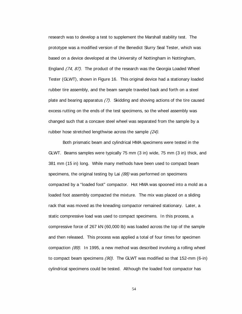
54
research was to develop a test to supplement the Marshall stability test. The
prototype was a modified version of the Benedict Slurry Seal Tester, which was
based on a device developed at the University of Nottingham in Nottingham,
England (74, 87). The product of the research was the Georgia Loaded Wheel
Tester (GLWT), shown in Figure 16. This original device had a stationary loaded
rubber tire assembly, and the beam sample traveled back and forth on a steel
plate and bearing apparatus (7). Skidding and shoving actions of the tire caused
excess rutting on the ends of the test specimens, so the wheel assembly was
changed such that a concave steel wheel was separated from the sample by a
rubber hose stretched lengthwise across the sample (24).
Both prismatic beam and cylindrical HMA specimens were tested in the
GLWT. Beams samples were typically 75 mm (3 in) wide, 75 mm (3 in) thick, and
381 mm (15 in) long. While many methods have been used to compact beam
specimens, the original testing by Lai (88) was performed on specimens
compacted by a “loaded foot” compactor. Hot HMA was spooned into a mold as a
loaded foot assembly compacted the mixture. The mix was placed on a sliding
rack that was moved as the kneading compactor remained stationary. Later, a
static compressive load was used to compact specimens. In this process, a
compressive force of 267 kN (60,000 lb) was loaded across the top of the sample
and then released. This process was applied a total of four times for specimen
compaction (89). In 1995, a new method was described involving a rolling wheel
to compact beam specimens (90). The GLWT was modified so that 152-mm (6-in)
cylindrical specimens could be tested. Although the loaded foot compactor has

55
been used to compact cylindrical specimens, the SGC is used most often for
preparing this type of specimen (91).
Samples tested in the GLWT were tested in the dry condition, so no
moisture damage information could be obtained from this test. The steel concave
wheel applied a load of 445 N (100 lb) to the sample, and the rubber hose was
pressurized to 690 kPa (100 psi). Test specimens were tracked back and forth,
allowing the stationary wheel to apply the load. Testing temperatures range from
30 C (86 F) to 60 C (140 F). Original work by Lai (88) was performed at 35 C (95
F), which was selected because it was the mean summer air temperature in
Georgia. The most common test temperature, however, was 40 C (104 F) (92).
Subsequent GLWT test temperatures have continued to increase (24).
The GLWT was typically conducted to a total of 8000 cycles, where one
cycle is equal to two wheel passes. A slotted template and micrometer was used
to measure deflection at seven to thirteen locations along the length of the sample
before and after the test. Final rut depth was defined as the average difference in
specimen profile before and after testing (24). Rut depths were compared with
maximum rut depth criteria of either 4.0 mm (0.16 in) or 7.5 mm (0.3 in) (92).
Asphalt Pavement Analyzer
The Asphalt Pavement Analyzer (APA) is a modification of the GLWT, first
manufactured in 1996 by Pavement Technology, Inc. The APA, shown in Figure
17, has been used to test for not only rutting, but also fatigue and moisture
damage. Unlike the GLWT, samples in the APA can be submerged during testing.
Another major difference is that in the APA, samples remain stationary with a

56
pressurized hose placed on top of each sample, and the wheels travel back and
forth across the samples (24). The APA is the primary LWT used in the
southeastern United States.
In the APA, three samples can be tested simultaneously. Either beams or
pairs of cylindrical specimens can be tested, and are usually compacted to a target
air void content of either 4.0 or 7.0 percent (91). Beams may be compacted with
either a vibratory or kneading compactor, and are typically 125 mm (5 in) wide,
300 mm (12 in) long, and 75 mm (3 in) thick. Cylindrical specimens are
compacted in the SGC to a height of 75 mm (3 in) and a diameter of 150 mm (6
in) (24). Field-compacted specimens can also be tested if trimmed to the
appropriate dimensions. Samples are secured within form-fitting acrylic blocks
during testing.
The APA typically uses the same wheel load and hose pressure as the
GLWT, which is a wheel load of 445 N (100 lb) and a hose pressure of 690 kPa
(100 psi). However, hose pressures can reach as high as 120 psi (828 kPa) and a
load as great as 1112 N (250 lb) can be accommodated. The wheel travels at a
speed of 0.6 m/s (1.97 ft/s), so an 8000 cycles test last approximately 2.5 hours
(83, 93).
In order to test for moisture susceptibility, samples must be tested for
rutting in both the wet and dry condition. Samples tested in the wet condition are
to be pre-conditioned in accordance with AASHTO T283 before being tested for
rutting (94).

57
APA test temperatures are now typically at or slightly above expected high
pavement temperatures rather than air temperatures (78). In fact, many states
use the standard high pavement temperature as recommended in the Superpave
design procedure for the particular geographic region. For most of the
southeastern U.S., the test temperature is 64 C (147 F) (72).
During testing, data is collected by the Automated Vertical Measurement
System (AVMS) of the APA. Twenty-five cycles are used to “seat” the wheel and
establish a zero reference point for subsequent measurements. During the test,
average rut depth is plotted versus the number of cycles. A typical plot of
resulting data from the APA appears as a smooth curve, unlike the typical HWTD
data plot. A typical data plot from the GLWT is shown in Figure 18.
Manual measurements are also taken using a slotted template and
micrometer to measure deflection before and after testing. For beam samples,
five points along the longitudinal profile of the sample are measured, and for pairs
of cylindrical samples, four points are measured. The average rut depth at the
end of the test is calculated and compared with maximum rut depth criteria.
Users have discovered some discrepancy between the automatic and manual
measurement (72). One study reported the difference in measurement methods
of approximately 2 percent (95).
Agencies are currently using maximum rut depth criteria from as little as
3.0 mm (0.12 in) to as much as 8.0 mm (0.32 in). The criteria are sometimes
dependant on the expected level of traffic for the mix (72). The repeatability of
the APA has been reported to be both acceptable (7) and unacceptable (23).
58
Accelerated Loading Facility
In the late 1980s, the Association of Australian State Road Authorities
(AUSTROADS) joined the asphalt industry in a joint research program through the
Australian Asphalt Pavement Association (AAPA) to improve the performance
quality of asphalt mixtures. An accelerated loading facility (ALF) was used to help
improve the rut resistance of HMA. In addition to the Australia, ALFs also operate
in the United States and China (96).
The ALF used by FHWA is a duplicate of the Australian model. It is a full-
scale pavement testing facility with programmable load distribution to simulate
actual unidirectional, non-uniform traffic patterns. ALF is a mobile, relocatable
road testing machine that applies full-scale rolling wheel loads to a 9.8 m (32.2 ft)
long test pavement (84). The load, which can be varied in 10 kN (1 ton)
increments between 40 and 80 kN (4 and 8 tons), tracks linearly and is guided by
the structural frame. The load is applied in one direction only, with the wheel
being lifted off the pavement at the end of the cycle and supported by the frame
upon its return. The structural frame is 29 m (95.1 ft) in length, containing a
moving wheel assembly that is capable of applying either dual-wheel or single-
wheel half single axle loading. The wheel loading can either be channelized or
applied over a normal transverse distribution 1.4 m (4.6 ft) or 1.0 m (3.3 ft) wide.
This distribution incorporates the aspect of wheel wander in order to more
realistically simulate field wheel load patterns. In most cases, ALF operates with
the narrow transverse loading distribution, which is ± 150 mm (6 in) of wheel
wander from the centerline (96).

59
The wheel travels at a speed of 18 km/hr (11.2 mi/hr) such that
approximately 380 load cycles can be applied each hour, and about 50,000 wheel
passes can be applied per week (84, 96). A rut depth of 20 mm (0.8 in) is defined
as the failure point (84).
Due to the considerable size and expense of an ALF, it is not a practical for
use in a laboratory for routine mixture design or quality control. It may, however,
be a valuable tool for validating the use of laboratory-scale LWTs.
Model Mobile Load Simulator
The one-third scale Model Mobile Load Simulator (MMLS3) was recently
developed in South Africa for testing HMA mixes either in the laboratory or in the
field. This device is similar to the full-scale Texas Mobile Load Simulator (TxMLS),
but scaled in size and load. The MMLS3, shown in Figure 19, is a unidirectional,
vehicle-load simulator for accelerated testing of model or full-scale, dry and wet
pavements. Six MMLS3 machines are currently operational, and have been used
in the United States, South Africa, and Switzerland (97).
The MMLS3 is 2.4 m (7.8 ft) long by 0.6 m (2 ft) wide by 1.2 m (4 ft) high.
It tests slab samples that are approximately 1.2 m (47 in) in length and 240 mm
(9.5 in) in width. The MMLS3 applies a scaled load on 300 mm (12 in) diameter
pneumatic tires that are about one-third the diameter of standard truck tires. It
has four wheels with a distance between centerlines of 1.05 m (3.4 ft). The wheel
load is approximately one-ninth the load of one wheel of a dual tire standard
single axle (97). Wheel wander can be incorporated into the test.

60
An environmental chamber can be placed around the device for control of
climatic conditions. Dry tests have been performed at 50 C (122 F) and 60 C (140
F), and wet tests have been performed at 30 C (86 F) (24). A maximum of 7200
single-wheel loads can be applied per hour, which equates to approximately 21
km/hr (13 mi/hr). Transverse profile rut depth measurements are used to
evaluate rutting potential. Criteria for the device are currently being developed
(97).
Superfos Construction Rut Tester
A device similar to the HTWD has been built by a private sector company.
The Superfos Construction Rut Tester (SCRT) was developed by Superfos
Construction, U.S. (previously Couch, Inc.) (81). The SCRT tests beam specimens
with dimensions similar to that tested in the HWTD. The primary difference
between the HWTD and the SCRT is the loading mechanism. The SCRT applies an
82.6 kg (180 lb) vertical load onto a solid rubber wheel with a diameter of 194 mm
(7.6 in) and a width of 46 mm (1.8 in). The result of this loading configuration is
a contact pressure of approximately 940 kPa (140 psi) and a contact area of 8.25
cm2 (1.28 in2). The wheel speed is approximately 556 mm/sec (21.8 in/sec). Test
temperatures in the SCRT range from 45 C (113 F) to 60 C (140 F), the most
recent research being performed at a temperature of 60 C (140 F) (98). Results
of the SCRT test include are creep slope, stripping slope, and stripping inflection
point.

61
PURWheel
PURWheel was developed at Purdue University as a tool to evaluate rutting
potential and/or moisture sensitivity. PURWheel is very similar to the HWTD, but
it can incorporate wheel wander into the testing. This feature is unique among
this type of laboratory-scale wheel tracking devices in the Unites States (24).
PURWheel tests slabs that have either been cut from the roadway or
compacted in the laboratory. Laboratory-compacted samples are compacted using
a linear compactor also developed at Purdue University. The slab compactor is
similar to the typical linear kneading compactor, but can compact larger
specimens. Typical slabs tested in PURWheel are 290 mm (11.4 in) wide by 310
mm (12.2 in) long. Sample thicknesses vary according to mix type. A sample
thickness of 38 mm (1.5 in) is used to test surface mixes, 51 mm (2 in) is used to
test binder mixes, and 76 mm (3 in) to test base mixes. Samples are compacted
to a target air void content of 7 ± 1 percent (24).
PURWheel employs a pneumatic tire at a pressure of 793 kPa (115 psi) to
apply a load of 175 kg (385 lb). The resulting contact pressure is approximately
620 kPa (90 psi). The wheel travels at a rate of 332 mm/sec (13 in/sec); and
samples can be tested either dry or submerged. A typical test lasts 20,000 wheel
passes or until 20 mm (0.8 in) of rut depth has accumulated.
Both rutting and stripping data can be obtained from the PURWheel device.
Moisture sensitivity is defined as the ratio of the number of cycles to 12.7 mm (0.5
in) of rutting in a wet condition to the number of cycles to 12.7 mm (0.5 in) of

62
rutting in the dry condition. The 12.7-mm (0.5-in) rut depth is used to
differentiate between good and bad performing mixes with respect to rutting (99).
SWK/UN
The SWK Pavement Engineering/University of Nottingham (SWK/UN)
wheel-tracking program uses a steel wheel similar to the HWTD that is 201.6 mm
(7.9 in) in diameter and 50.4 mm (2 in) in width. No preconditioning load is
applied, but the test itself lasts 500,000 passes with a wheel loaded at 181 N (41
lb). Fifty wheel passes per minute are applied to samples being tested submerged
in water at a temperature of 40 C (104 F) (100).
OSU Wheel Tracker
Oregon State University owns a LWT that loads the sample with a
pneumatic tire, similar to that of the FRT. A preconditioning load of 50 wheel
passes is applied, and then the actual test begins. Samples are tested for 10,000
wheel passes under a 726-kg (1600-lb) load, which creates approximately 690 kPa
(110 psi) of actual contact pressure. The wheel applies 60 cycles per minute,
which is equivalent to 120 wheel passes per minute. Tests are performed at 40 C
(105 F) (100).
Utah DOT Wheel Tracker
The Utah Department of Transportation (UTDOT) has obtained a wheel
tracking device that is very similar to the HWTD. This device was purchased from
Copper Unlimited located in England (101).
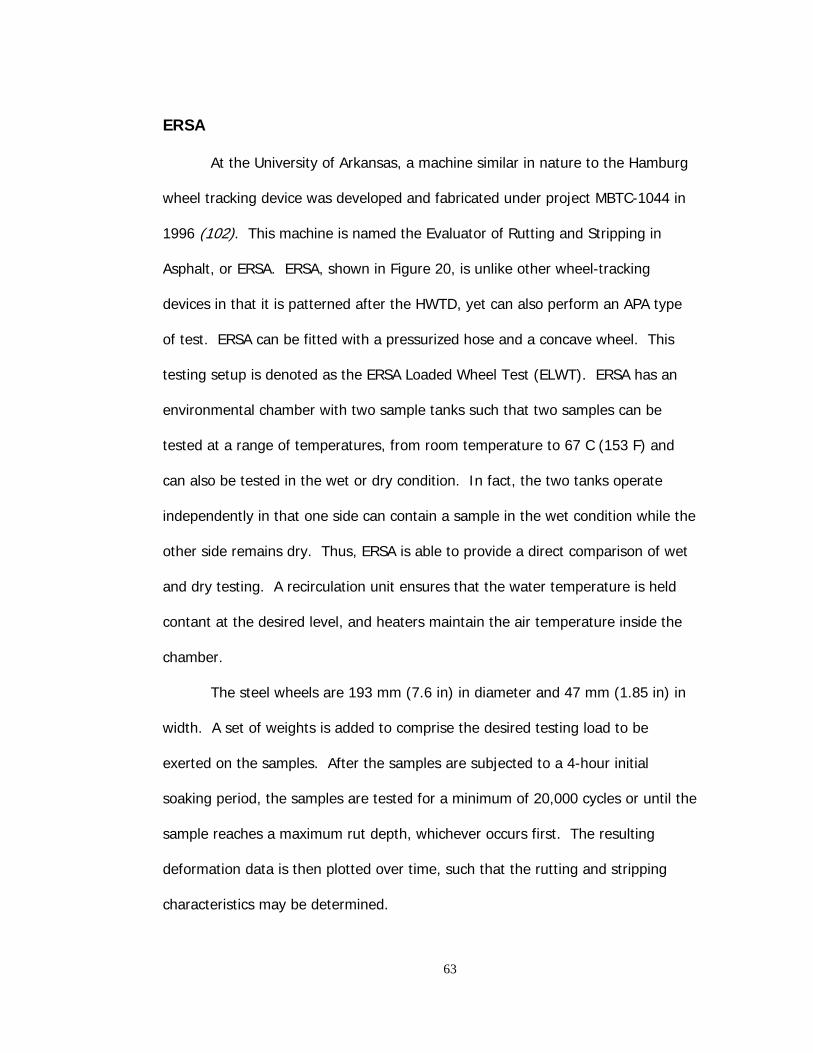
63
ERSA
At the University of Arkansas, a machine similar in nature to the Hamburg
wheel tracking device was developed and fabricated under project MBTC-1044 in
1996 (102). This machine is named the Evaluator of Rutting and Stripping in
Asphalt, or ERSA. ERSA, shown in Figure 20, is unlike other wheel-tracking
devices in that it is patterned after the HWTD, yet can also perform an APA type
of test. ERSA can be fitted with a pressurized hose and a concave wheel. This
testing setup is denoted as the ERSA Loaded Wheel Test (ELWT). ERSA has an
environmental chamber with two sample tanks such that two samples can be
tested at a range of temperatures, from room temperature to 67 C (153 F) and
can also be tested in the wet or dry condition. In fact, the two tanks operate
independently in that one side can contain a sample in the wet condition while the
other side remains dry. Thus, ERSA is able to provide a direct comparison of wet
and dry testing. A recirculation unit ensures that the water temperature is held
contant at the desired level, and heaters maintain the air temperature inside the
chamber.
The steel wheels are 193 mm (7.6 in) in diameter and 47 mm (1.85 in) in
width. A set of weights is added to comprise the desired testing load to be
exerted on the samples. After the samples are subjected to a 4-hour initial
soaking period, the samples are tested for a minimum of 20,000 cycles or until the
sample reaches a maximum rut depth, whichever occurs first. The resulting
deformation data is then plotted over time, such that the rutting and stripping
characteristics may be determined.

64
ERSA is capable of accommodating a variety of sample types. The two
primary shapes are cylindrical cores and prismatic beams, or slabs. One beam or
slab can be tested in a sample tray. If 150-mm (6-in) cylindrical cores are used,
then two are placed next to each other lengthwise (See Figure 13). Regardless of
specimen configuration, ERSA sample trays are able to receive samples up to 175
mm (7 in) in depth, 380 mm (15 in) in length, and 300 mm (12 in) in width. This
is considerably larger than most other laboratory-scale wheel tracking devices.
A complete test of 20,000 cycles lasts just over 18 hours. The sequence of
specimen preparation, submerging and heating, and finally the actual test, dictates
a testing schedule of 3 days per test (consisting of two samples). Assuming that
the stages of specimen preparation and sample testing overlap, one ERSA test can
be performed each day.
A computer-based data acquisition system employs linear variable
differential transducers (LVDTs) to collect vertical deformation measurements at
75 locations along the profile of the sample. The frequency of data recording can
be adjusted to any desired interval. ERSA currently records deformation data at
thirty-minute intervals, which allows the volume of data to be reduced to a
manageable size while allowing adequate information to develop a deformation
curve over time as well as sample profiles. The plot of deformation versus
number of cycles results in a plot similar to that of the HWTD data, which is given
in Figure 14. The data resulting from an ERSA test includes initial consolidation,
rut depth, rutting slope, stripping slope, and stripping inflection point.

65
Road Tests
Because wheel-tracking tests are empirical, they must be calibrated to
agree with actual field performance. This can be done by comparing wheel-
tracking results to field rutting measurements. While this would be a reliable
method, it takes many years to develop long term performance data. A preferable
option is to compare wheel-tracking test results to pavement performance road
tests. Road tests are pavement sections that are loaded at an accelerated rate so
that long term results can be obtained in a short amount of time. Traffic loading
and environmental conditions are realistic, and pavement responses are carefully
monitored. The materials and construction conditions are known, so the
responses can be related to the original conditions. One advantage of a road test
is that a tremendous amount of data can be collected. The disadvantage is that
the correlations that develop are only valid for the materials and conditions at that
particular site. A benchmark road test for flexible pavement design was the
AASHO Road Test, performed in the early 1960s near Ottawa, Illinois (18).
Recently, the National Center for Asphalt Technology (NCAT) Test Track was built
in Alabama (103). The 2.8 km (1.7 mi) oval track contains 46 pavement sections,
each one 61 m (200 ft) in length. Other road tests include a circular test track in
Nantes, France, and WesTrack in Nevada.
WesTrack
The Federal Highway Administration (FHWA) and the National Cooperative
Highway Research Program (NCHRP) sponsored the WesTrack project, which is a
$15 million, full-scale test track facility located in northern Nevada. Its purpose is

66
to further the development of performance-related specification (PRS) systems for
flexible pavements (104). WesTrack consists of 26 HMA test sections that were
used to simulate typical construction variability and its effect on pavement
performance. Gradation, binder content, air-void content, and the percent passing
the 0.075 mm (#200) sieve were varied for an angular aggregate source mixed
with a PG 64-22 binder, and compacted to a six-inch thickness. Models were
developed that include the performance characteristics of fatigue cracking,
permanent deformation, and thermal cracking, among others. Neither empirical
nor mechanistic models were sufficient, so mechanistic-empirical models are the
most likely candidates; however, the models may be too complicated for use in
the PRS (105).

67
CHAPTER 3
LITERATURE REVIEW

68
PERMANENT DEFORMATION
Rutting due to shear failure has not been adequately modeled in the past.
Superpave performance-related tests were intended to be a solution to this
problem. In the SHRP–A/IR-91-104 report (106), the repeated load simple shear
test was given the highest ranking as compared to the other methods tested for
assessing resistance to permanent deformation. Wheel-tracking tests were not
ranked well. However, the SHRP performance models have not proven to provide
reasonable performance predictions (107). Continued research is being performed
using the SST and other similar devices to develop permanent deformation
relationships. Tests such as the triaxial (or axial) and simple shear tests are
considered more fundamental than laboratory-scale wheel-tracking tests (35).
However, until such relationships are developed, wheel-tracking tests are being
used as an empirical method for predicting relative rutting performance. Wheel-
tracking tests have the advantages that the stress state applied to the sample is
similar to that occurring in the field, and it is relatively inexpensive and easy to
operate. The disadvantage is that no resilient modulus is obtained from the test
(74).
Rutting Tests
Before wheel-tracking tests can be correlated with actual field
performance, the effects of critical test parameters must be established. It may
be assumed that because all LWTs operate under the same basic principle, the
effects of various test parameters and material constituents should be similar to
each (24). However, the loading mechanisms and testing configurations of the

69
LWTs are all slightly different, so this assumption may be false. Test parameters
and materials that may affect the results of the LWT tests include air void content,
temperature, load, sample shape, compaction method, and mixture
characteristics. Similar parameters could also affect more fundamental tests, such
as those performed in the SST.
Air Void Content
The air void content of samples to be tested in LWTs is usually specified by
the test method to be either 4 or 7 percent. Specified air void contents are usually
based on one of two ideas. Some are in favor of 7 percent because it is more
representative of the density of a newly constructed pavement. Others favor 4
percent air voids, because shear failure of mixes has been shown to occur in
pavements of less than 3 percent air voids (34, 36, 108). In general, LWT rut
depths increase as air voids increase (91, 109). Air void content is typically a very
significant factor influencing a material’s sensitivity to rutting. Generally, a
material is most stable at some air void content between 3 and 7 percent. Below
3 percent and above 7 percent, the likelihood of rutting increases. To avoid this
phenomenon, the HMA should be compacted to an air void content above 3
percent, preferrably 5 to 7 percent, using an adequately high compactive effort so
that the voids remain above 3 percent even under expected traffic. The degree to
which such air voids affect rutting susceptibility is a function fo the stability of the
material.
This concept is illustrated by tests performed in North Carolina based on
known field performance (110). Field cores were cut from the roadway, broken

70
down, then recompacted by the Marshall hammer. The recompacted samples of
mixes showing field rutting contained air voids of less than 3 percent, which is
outside the specification limits of 3 to 5 percent. Field cores from mixes showing
field rutting also contained less than 3 percent air voids in the wheel path. Field
cores from mixes showing no field rutting contained slightly more than 3 percent
air voids in the wheel path.
In the APA, samples should be compacted to 7 ± 1 percent air voids. The
ruggedness study found that the APA is very sensitive to air void content (109). It
has since been suggested that the target sample air void tolerance be reduced,
such that samples should be compacted to 7 ± 0.5 percent air voids (72).
Air voids was supected to be a significant factor in the HWTD. However,
for the mixes tested by the Colorado DOT, the rutting slope remained essentially
the same for different air voids contents. Some tests indicated that for air void
contents greater than ten percent, the stripping inflection point occurred at a
smaller number of passes than for samples compacted to six or seven percent air
voids. The resulting recommendation was that samples for the HWTD should be
compacted to an air void content of 6 ± 1 percent, because the stripping inflection
point was not significantly impacted by air voids in this range (79).
Repeated load axial (RLA) tests were performed using the Nottingham
Asphalt Tester (111). No consistent effect of a wide range of air voids on the
accumulated strain was evident for any of the materials tested.

71
Temperature
Test temperature is usually one of the parameters specified for a
permanent deformation test. Due to the change in behavior of asphalt binders at
different temperatures, it would be expected that temperature is a significant
factor with regard to laboratory rutting performance. It is logical that as the
temperature increases, rut depth would also increase. This hypothesis has been
proven to be true in several studies (37, 91, 92).
Temperature has been a popular topic of discussion with regard to the
GLWT and APA tests. Original work done by Lai (88, 112) was performed at 35 C
(95 F), which was selected because it is the mean summer air temperature in
Georgia. Since that time, test temperatures in the GLWT have continued to
increase. APA test temperatures are now typically at or slightly above expected
high pavement temperatures, as opposed to air temperatures (78). The SHRP
environmental effects model allows pavement temperatures to be accurately
determined from air temperatures. According to the model, pavement
temperatures are approximately 30 to 35 C (54 to 63 F) higher than air
temperatures on hot summer days. The original GLWT testing was performed
based on air temperatures, but should more accurately model field conditions if
tested at actual pavement temperatures. Research in Wyoming indicated that a
40.6 C (105 F) test temperature may not be severe enough to predict pavement
rutting. The test temperature was increased to 46.1 C (115 F) in order to
correlate with field performance (7). Current test temperatures being used in the
southeastern U.S. are in the neighborhood of 64 C (147 F) (72, 113).

72
Because so much rutting data had been collected from GLWT tests at lower
temperatures, a temperature effects model (TEM) was developed as a method for
predicting test results at a different temperature and number of loading cycles
than was actually used (92). As a result, historical data for mixes tested at lower
temperatures can be converted to useful data based on current test temperature
recommendations. Also, an abbrebiated test can be performed and the results
predicted as if the full-length test had been completed, thereby shortening the
testing time for each sample. Five dense-graded HMA mixes and two stone-matrix
apshalt (SMA) mixes were used to develop the TEM. One type of binder was used
and only beam samples were tested. In order to normalize the model for a variety
of mix parameters, an asphalt mixture characteristics parameter (RO) was
introduced. This factor accounts for the actual rutting for that particular mix at its
particular test parameters. The basic model is given in Equation 4:
[R/RO] = [T/TO]α [N/NO]β Equation 4
where R = predicted rut depth,
RO = reference rut depth obtained from the GLWT test at the
reference conditions TO and NO,
T and N = temperature and number of load cycles at which the
rut depth is sought,
TO and NO = reference temperature and load cycles at the RO,
α, β = statistically determined coefficients.
The test parameters established for dense-graded HMA in the TEM were α
= 2.625 and β = 0.276. Only 7 out of 170 predicted values deviated from

73
measured values by more than 0.8 mm, the maximum deviation being 1.1 mm.
The test parameters established for the SMA mixes were α = 2.860 and β =
0.313. Only 2 out of 64 predicted values deviated from measured values by more
than 0.8 mm, the maximum deviation being 1.0 mm. Based on the equations, it
appears that SMA mixtures are more sensitive to temperatures and load
repetitions than that of the dense-graded HMA. The SMA mixtures exhibited much
less rutting than the dense-graded HMA used in this study.
Temperature in the HWTD and FRT has also been determined to be a
significant factor. A study in Colorado determined that test temperature was
significant with respect to both rutting and stripping in the HWTD (79). A later
study was performed in the HWTD using a variety of asphalt binders having a
range of stiffness properties (76). The HWTD test results were compared to
actual field performance. Depending on climate, softer or stiffer binders may be
recommended. It was suggested that test parameters should be chosen such that
the wheel-tracking test would not penalize softer binders in colder regions. The
environmental conditions for the HMA mixture should be considered when the
testing temperature is chosen. In general, for each grade increase of binder, the
test temperature should increase by about 6 C in order to effect the same
stripping inflection point. The temperature differential required by the HWTD to
produce equivalent stripping performance in different binder grades was almost
identical to that measured by the DSR (76). In order to correlate with the German
procedure, the high temperature performance asphalt cement grade of 64 or 70
should be tested at 50 C (122 F), and binders with a high temperature grade of 76
74
should be tested at 55 C (131 F) (79). Research in Texas suggests that a test
temperature of 50 C (122 F) may too severe for mixtures containing AC-20
binders. The AC-20 classification of binder is roughly equivalent to a performance
graded binder of PG 64-22 (17).
Temperature was found to have a significant effect in the FRT as well.
When a relatively rut-resistant mix was tested at 50 C (122 F) and at 60 C (140 F),
equivalent rut depths were noted at a number of cycles that differed by a factor of
ten. In other words, the percentage of rutting at 50 C (122 F) and 100,000 cycles
was the same as for a test temperature of 60 C (140 F) and 10,000 cycles. A less
rut resistant material may exhibit this same type of characteristic for even smaller
variations in temperature, such as 5 C (9 F) (36). Research was performed to
compare the FRT predictions to pavements of known performance. The typical
test temperature of 60 C (140 F) for the FRT was considered too severe for typical
pavements in Colorado (85). Therefore, it was recommended that the severity of
the test be lessened in order to better correlate with field performance in colder
regions (82).
Results of another study indicate that G* increases with decreased
temperature. However, this relationship was shown to be nonlinear, such that the
variability in G* is largest at low temperatures (42).
Load
Similar to expectations for increases in temperature, it would be expected
that increasing the load in a LWT would increase the resulting rut depths. For
significant increases in load, this theory was proven to be true for the APA test

75
(88). However, small changes in the magnitude of the load did not produce
significantly different rut depth results (109). Some studies have suggested that
increasing the typical 445 N (100 lb) load to 533 N (120 lb) increases the
discrimination of the APA test (78). In an ongoing NCHRP study, the effects of
increasing various parameters in the APA are being analyzed, including a higher
load of 533 N (120 lb), a higher hose pressure of 828 kPa (120 psi), and even a
larger hose diameter of 38 mm (1.5 in) (72). Nothing was found in the literature
regarding variations in test load for the HWTD or FRT methods.
Sample Shape
Most LWTs were developed to test beam specimens, but since the
Superpave mix design specifies the use of the SGC for compacting laboratory
samples, it seems that testing 150 mm (6 in) cylindrical specimens could be a
more efficient process. Also, not all mix design laboratories possess a slab
compactor. Using SGC specimens would reduce the expense related to LWT
testing.
A Florida research team (23) investigated the effect of specimen shape for
laboratory-compacted samples tested in the APA. The results indicated that the
magnitude of rut depth for the two shapes were not statistically similar, but that
they did provide equivalent rankings of the mixes. When rut depths were less
than 10 mm (0.4 in), the gyratory-compacted samples were less resistant to
rutting.
Other studies have supported this conclusion. A ruggedness study of the
APA included results regarding compaction method of sample specimens (109). A

76
study in Texas involving the HWTD also addressed this issue (54). In both
studies, slab and cylindrical specimens ranked mixes similarly, but did not
necessarily produce equivalent rut depths and stripping inflection points. The
Texas study stated that performance for slabs and cylinders was statistically
similar with regard to rut depth, but not stripping inflection point. The SGC
specimens were more resistant to moisture damage. Also, the slab samples
exhibited a higher variability than the SGC specimens. These results do not imply
that one method of compaction is better than another, but simply that a
compaction method should be specified if results are to be compared directly.
The difference in performance of laboratory-compacted slabs and
cylindrical specimens is likely due to the difference in compaction mechanisms
used to create the two sample shapes. The method of compaction influences the
density gradient and aggregate orientation within the samples, thereby creating
different levels of rutting resistance (114). If one compaction method can be
proven to better correlate with field results, it should be the method specified.
However, nothing in the literature has addressed this idea.
Another consideration regarding sample shape involves the use of paired
cylindrical specimens in HWTD testing. The width of the steel wheel is such that it
does not maintain complete contact with the HMA specimens at the intersection of
the two cylinders. To correct this, flat faces can be sawn on the specimens so
that they “butt” up against each other, as shown in Figure 21. Testing in Texas
indicates that HWTD test results from the two configurations rank mixes similarly
(54). Cut and uncut specimens were also tested in the RSCH test (42). No trend

77
was apparent regarding the specimen configuration relative to the number of
repetitions to a given permanent shear strain.
Compaction Method
Since slab and cylindrical specimens may produce different test results with
regard to permanent deformation and the only real difference between the two
sample types is method of compaction, it would seem reasonable that the
compaction method would be a significant factor. In fact, this is the case. Studies
have compared laboratory-compacted specimens to field-compacted specimens
(42, 76). In one study, rutting performance was tested by the RSCH method in
the SST. Another study tested samples in the HWTD. Both assessments indicate
that laboratory-compacted specimens are more resistant to permanent
deformation than field-compacted cores. SGC-compacted specimens produce
different aggregate and voids structures between the internal portion and outer
edges of the specimen (115). Thus, aggregate orientation and distribution, as
well as interactions between the binder and aggregate are probably responsible.
Another possibility for the difference in lab and field compaction is that even
though average air void contents for the laboratory and field specimens may
match, the densely compacted central portion of the SGC specimens may be
providing increased rutting resistance (42). Permanent shear resistance increases
considerably with increased compaction.
In addition to compaction method, compaction temperature may also be
significant. Using the HWTD, it was determined that higher compaction
temperatures were related to increased rut resistance. However, this could be

78
due to the fact that all samples in the study, regardless of compaction
temperature, were compacted to the same air void content. Therefore, greater
compactive effort was required to achieve density at lower temperatures. When
this happens, aggregates may break, microcracks can develop in the HMA, or the
air voids could be interconnected (76). A similar study in the APA was performed
by Pavement Technology, Inc. (PTI) (116). In this study, a range of temperatures
from 93 C (200 F) to 149 C (300 F) were used, but not all samples possessed the
same air void content. Compaction level was held constant such that as the
compaction temperature decreased, the air void content increased. The test
results showed that as compaction temperature increases and air void content
decreases, the rutting resistance of the mix increases. Rut depths in the APA are
known to be sensitive to sample air void content (109). Therefore it is unknown
whether the change in rutting resistance is due to the compaction temperature or
the air void content of the samples.
Samples tested in the FRT are typically in the form of slabs. The slabs can
be compacted by a variety of compactors. Testing results showed that samples
compacted with the linear kneading compactor gave slightly better results than
samples compacted with the French plate compactor, which compacts the sample
using a pneumatic tire (76).
Test Type
For virtually all forms of LWTs, there is some level of useful correlation
between LWT test results and mixture rutting potential. LWT devices provide a
ranking or a pass/fail recommendation based on set criteria rather than predicting

79
a specific measure of future rut depth (24). Because empirical relationships are
used, test results must be correlated with field performance and/or accelerated
pavement testing results.
In a 1997 study, a laboratory-scale wheel track tester was validated using
the ALF (96). There was a reasonable correlation and it was concluded that LWTs
could be used as a surrogate method for the ALF. In the same study, G*/sin δ of
the mixture was compared to the ALF. No clear correlation was determined
between the two. In fact, “tan δ” was a better indicator of performance in the
ALF. In another study, the FRT, GLWT, and HWTD were tested in comparison to
the ALF (117). The LWTs did not always rank the mixtures in the same manner as
the ALF. One of these studies concluded, “No laboratory mixture test clearly stood
out as the best test based on comparisons to the statistical ranking for ALF
pavement performance…” (117).
In a joint study by FHWA and the Virginia Transportation Research Council,
results from the same three LWTs (HWTD, APA, and FRT) were compared to the
performance of pavements at WesTrack (78). The APA was performed at a 533 N
(120 lb) load and a hose pressure of 828 kPa (120 psi) in order to improve the
discrimination of the test. There was a strong relationship for all three of the
LWTs, the HWTD having the highest correlation (R2=0.91), the APA having the
next highest correlation (R2=0.90), and finally the FRT (R2=0.83). These
correlations are considered to be excellent, and are quite higher than those
reported in a previous study (118). Previously, the correlations were 76.2 percent
for the HWTD, 43.6 percent for the APA, and 57.4 percent for the FRT. The

80
MMLS3 has also been reported to provide accurate pavement rankings based on
WesTrack performance (97).
A recent study compared the evaluations of mixes with respect to
permanent deformation as determined by the SST and the HWTD (11). Mashall
and Superpave mixes containing a PG 64-22 binder and a sandstone aggregate
were used. RSCH and HWTD (at 40 C) tests were performed. The results showed
that the Superpave mixes were less susceptible to permanent deformation than
the Marshall mixes. Also, the results of the HWTD tests were consistent with the
RSCH tests. Creep characteristics were evaluated by the FSCH test. The creep
compliances for the mixes tested could not successfully predict the pavement
performance in comparison with the RSCH and HWTD. Another source also
suggests that repeated loads, rather than creep loading, should be used to
determine the susceptibility of a mix to rutting (20). The dynamic creep tests
were, however, able to rank mixes similar to the FRT according to performance on
the circular test track of the LCPC (43).
RSCH test results have also been compared with APA results. Three
aggregates with varying gradations were tested. The shear strain obtained from
the SST does not appear to be as sensitive to gradation differences as the APA,
but similar indications were obtained with regard to rut depth (13).
The SST has been reported to provide valuable information regarding the
rutting resistance of HMA mixes. The SST, however, is expensive to own and
operate. The rapid triaxial tester, when compared to the SST, was better able to

81
distinguish between mixes. Test results also compared well to field rutting
behavior after three years of service (119).
In a Texas study, four WesTrack mixes were ranked according to
performance in the RSCH, HWTD, APA, and static creep test. The RSCH and
HWTD were able to correctly rank the mixes, but the APA and static creep tests
did not (97).
In North Carolina, the RSCH at Superpave 50 percent reliability
temperatures, the FRT at 60 C (140 F), and the GLWT at 40.6 C (105 F) were
used to test field samples of known performance (110). The RSCH most closely
matched field rutting measurements. Performing the GLWT at a higher
temperature could possibly improve its relationship with field performance.
Criteria
The criteria set by the Germans for the HWTD device is a maximum rut
depth of 4 mm (0.16 in) after 20,000 wheel passes. This criteria was considered
too severe for Colorado pavements. Thus, a choice of two criteria was proposed.
The first was a maximum allowable rut depth of 10 mm (0.4 in) at 20,000 passes,
and the second was a maximum allowable rut depth of 4 mm (0.16 in) at 10,000
passes (120). The criteria currently used in most cases by the Colorado DOT is a
maximum allowable rut depth of 10 mm (0.4 in) at 20,000 passes (80).
Based on WesTrack performance, an arbitrary acceptable performance in
the HWTD would exhibit deformation at a rate of 0.001 mm per wheel pass. This
is equivalent to a rutting slope of 1000 passes/mm rut depth, meaning that no less
than 1000 wheel passes should create a 1-mm (0.04-in) rut depth. Based on

82
WesTrack information, this equates to approximately a 5.82-mm rut depth after
the application of 582,000 10-kip (44.48-kN) ESALs (78). Acceptable field rut
depths have been reported as small as 5 mm (0.2 in) and as large as 20 mm (0.8
in) (108, 30).
Criteria in the GLWT and APA vary according to the specifying agency.
One of the first measures of failure was defined as more than 7.6 mm (0.3 in) of
rutting after 8000 cycles (84). The states of Maryland and Utah have both used a
more limiting specification, such that the maximum allowable rut depth is 5.0 mm
(0.2 in) (113). At the 2000 APA User-Group meeting, maximum allowable rut
depths as low as 3.0 mm (0.12 in) were reported. Some states use a tiered
system in which the maximum allowable rut depth is related to the traffic volume
level for the mix, such that the specification is relaxed for lower traffic volume
mixes. A summary of criteria for participating states is contained in Table 2 (72).
Repeatability
The repeatability of the HWTD is acceptable, as this test method has been
established in Europe for several years. In 1998, a round robin study was
coordinated by the Texas Department of transportation to study the repeatability
of testing with the Hamburg and other similar wheel tracking devices (81). The
University of Arkansas participated in this study using ERSA. Samples of a gravel
mix and a limestone mix were each compacted to 7 ± 1 percent air voids, and
then tested submerged at a temperature of 50 C (122 F). It was determined that
for the gravel mix, which was a good performer, the repeatability among the
different laboratories was good. For the limestone mix, which was a poor

83
performer, the results from different laboratories held more variation. In general,
the Hamburg and similar devices were determined to have acceptable
repeatability, but those who used the device marketed by Helmut-Wind, Inc.,
exhibited a higher level of repeatability. Although previous research by the Texas
DOT indicated otherwise, one other conclusion of the round robin study was that
either cylindrical samples compacted in the SGC or slabs compacted in the
laboratory may be used to predict a level of performance. This was true for both
the gravel and the limestone mix (81, 101). It has also been shown that HWTD
tests are very repeatable when six replicates are used. There is no statistical
advantage to using more than six replicates (54, 78).
In order to determine the repeatability of the GLWT, a round robin study
was conducted. The results were affected by a difference in sample densities,
meaning that the air void content of the sample is a significant factor. Although
there was a difference in air voids, the overall reproducibility standard deviation
was 0.128 (121). The difference in air voids posed a problem in analyzing data
which suggested that laboratory-compacted cores and beams behave similarly in
the LWT (91, 122). Increased variability is exhibited for samples with poorer
performance. This is true for all types of LWTs. Although many have deemed the
GLWT and/or APA an acceptable laboratory tool (89, 124, 123, 124), the beam-to-
beam variability needs to be reduced (125), especially when rut depths exceed 10
mm (0.4 in) (109). Some feel that the APA testing variability is still too significant
to be used as a pass/fail criteria at the present time (23).

84
Mixture Characteristics
A number of studies have been performed to analyze the effects of asphalt
mixture properties on rutting performance. Asphalt binders can affect rutting
resistance. A binder content that is too high can reduce the effectiveness of the
aggregate skeleton and cause premature rutting. A binder content that is too low
can leave the aggregates thinly coated, making the HMA susceptible to stripping.
Intermediate course mixes may experience a decrease in rutting with an increase
in film thickness (126).
Binder grade can also affect rutting performance. In general, the higher
the binder grade, the stiffer the binder, and the greater the rutting resistance as
defined by G*/sin δ from the DSR test (37, 124). Several studies have indicated
that LWTs can differentiate between asphalt binder grades (37, 91).
The gradation of the aggregate blend in the HMA mixture can play a
significant role in resistance to permanent deformation. Specifically, the
percentage of aggregate passing the No. 40 sieve and the No. 80 sieve can
influence rutting. When a hump appears in this region of the gradation curve, the
mix is considered tender, or susceptible to premature rutting (58, 127).
Aggregate gradations passing through the restricted zone may be acceptable in
terms of rutting resistance even though the purpose of the restricted zone was to
minimize the likelihood of rutting (13). One study concluded that the Superpave
restricted zone should only be observed when a proof test is not available to
predict rutting performance (128). No clear trends have been found relative to
the type of gradation (i.e., above or below the restricted zone) (126).

85
Nominal maximum aggregate size can affect LWT results; typically mixes
with larger aggregates are more resistant to rutting (88, 123). In a study
involving the ALF and several laboratory-scale LWTs, only the ALF was able to
distiguish between mixes of different aggregate sizes (117).
Coarse and angular particles help to resist rutting. Coarse aggregate
angularity, measured as having two or more crushed faces, can increase rutting
resistance (34). Also, higher percentages of crushed aggregate can significantly
aid in rutting prevention (95).
Fine aggregates can increase the rutting susceptibility of a mixture, but
controlling the type of fine aggregate can maintain the rutting resistance of a mix
(129). Natural (rounded) sands increase a mixture’s susceptibility to rutting, but
angular fines can increase mix stability. A Missouri study using the GLWT
determined that rutting resistance can often be increased by increasing the
amount of fine aggregate passing the 0.300-mm (#50) and 0.150-mm (#100)
sieves (124).
In some cases, the rutting resistance of a mix can be enhanced more by
strengthening the aggregate gradation than by chaning the grade or amount of
binder (36). Stiff binders combined with large aggregates are optimal for creating
shear resistance (13).
Compaction characteristics can also provide information relative to a
pavement’s resistance to permanent deformation. In theory, the greater the
compactive effort required to compact a sample, the greater its shear resistance.

86
The concept of the gyratory ratio (the ratio of the number of gyrations required to
achieve two percent voids to the number of gyrations required to achieve five
percent voids) suggests that if a gyratory ratio is less than 4 then the mix might
be unstable (44). Nini and Nmax criteria have been specified by Superpave in order
to avoid tender mixes and mixes prone to rutting, respectively. If the density is
within 0.1 to 0.2 percent of 98 percent of Gmm at Nmax, rutting may be more
pronounced (126).
87
MOISTURE SUSCEPTIBILITY
Moisture damage has been tested by many methods, but none have
proven superior at predicting field moisture susceptibility (52). Common problems
reported with traditional moisture damage testing are that the pass/fail criterion is
qualitative, many determinations are subjective, field conditions are not simulated,
and there is low correlation with field data. For stripping due to the physio-
chemical incompatibility of the asphalt/aggregate system, it has been suggested
that classical moisture sensitivity tests are relevant. However stripping due to a
mechanical failure of the mix occurs when cyclic hydraulic stress physically scours
the asphalt binder from the aggregate. Classical moisture sensitivity test are not
relevant for this type of stripping (47). Stripping in wheel-tracking tests may be
due to the hydraulic scouring mechanism and/or excessive pore pressure caused
by the moving wheel (46). Since all mixes can fail due to mechanical stripping,
this type of test may be the most applicable for testing the moisture susceptibility
of a mix.
Visual Tests
Visual tests for moisture damage, such as the boiling water test and the
static-immersion test, have been used for many years. One study reported that
the boiling test criterion was too severe (63). These tests are not recommended
due to their subjectivity and lack of correlation with field performance (48).
Aggregate Tests
Because stripping can be a function of the aggregate, primarily plastic
fines, aggregate tests such as the methylene blue, sand equivalent, and dust
88
evaluations can provide valuable information regarding stripping. Two studies
reported that the MBVs correlated well with field stripping performance, although
marginal performers may not be detected (63, 67). Sand equivalent values did
not correlate with field performance. This study suggests that a combination of
aggregate tests including the methylene blue test, dust coating percentage, and a
measure of stiffening power could be useful in determining the cause of stripping.
If an HMA mix fails a performance-related stripping test, such as the HWTD, then
aggregate testing may provide some indication of the cause of stripping (67). The
sand equivalent and MBVs do not correlate well with TSR values (130).
Strength Tests
Strength tests such as the Modified Lottman, Lottman, and Root-Tunnicliff
methods subject a set of samples to a moisture conditioning process, and then
compare the strength of the set of conditioned samples to a corresponding set of
unconditioned control samples. Criteria can be based on either a measure of
retained tensile strength, retained resilient modulus, or a combination of the two
(49, 24). The Modified Lottman test (AASHTO T283) is thought to be fairly
successful at identifying very good and very poor performing mixtures, but it is not
necessarily capable of identifying marginal performers (63, 71).
Conditioning
Because stripping occurs in the presence of moisture, HMA samples
prepared in the laboratory must be conditioned before testing. Conditioning
samples is a way to model the environmental effects of moisture in the field. In
AASHTO T283, samples are subjected to a vacuum saturation process, and an

89
optional freeze thaw cycle. The target saturation level to be achieved in the
vacuum saturation process is 55 to 80 percent. If over-saturation results, the
samples may be damaged and must be discarded. However, in case histories
involving stripped aggregates, samples were near 100 percent saturation, not the
55 to 80 percent recommended by AASHTO T283 (47). Additionally, one study
determined that over-saturation did not damage samples. In fact, the
discrimination of the test was improved by using a 30 minute vacuum saturation
to create a higher level of saturation (131).
There is a relatively strong correlation between the saturation level and
measured TSRs in the AASHTO T283 test. Specifically, TSRs, decrease as the
saturation level increases. The optional freeze-thaw cycle also has a significant
effect on TSR values. AASHTO T283 was reported to have more potential for
predicting stripping potential if the saturation level is above 90 percent and a
freeze-thaw cycle is used. Also, stripping may be sensitive to air void content
such that as air voids increase, tensile strength decreases (71). Therefore the
requirement for test specimen compaction should be tightened to 7 ± 0.5 air voids
rather than 7 ± 1 percent (57).
In a study by FHWA, moisture sensitivities were predicted by ASTM D4867,
then compared to field performance. The study concluded that if the laboratory
samples had less than 6 percent air voids, they were not damaged enough in the
laboratory test, even if lower air void contents were measured in the field. The
same conclusion is true the AASHTO T283 (132). Correlations relating air voids to
stripping based on the Root-Tunnicliff test were very poor (49).

90
Survey of States
A 1989 survey of state highway agencies indicated that states are
concerned with stripping (48). Of 46 responding agencies, 34 indicated that
moisture damage is a significant problem. Arkansas and Utah reported an
estimated 20 to 30 percent of pavements experiencing moisture-related distress.
Only four states (Arizona, Idaho, Louisiana, and South Carolina) reported greater
percentages. The largest percentage of agencies responding indicated the use of
a retained tensile strength as an assessment of moisture damage.
The Environmental Conditioning System
AASHTO T283 is probably the most common measure of moisture damage
in the United States. More and more agencies moved to this method when the
SHRP research group chose it as the preferred moisture damage test in Superpave
mixture design. The Environmental Conditioning System (ECS) was developed
during SHRP in order to provide a quantitative measure of moisture susceptibility
while modeling field conditions (62). Validation testing showed the ECS to have a
reasonable correlation with field performance for a range of HMA mixes, but the
relationships were not as strong as had been hoped (130, 133). A study of
AASHTO T283 and the ECS were tested for accuracy and precision, and the results
were compared to known field performance (55). AASHTO T283 was reported to
yield more precise (repeatable) results as compared to the ECS procedure.
However, neither test was able to accurately discriminate between good and poor
performing mixes. Thus, the ECS was determined to be an reliable method.
Improvements were suggested involving the modification of the ECS conditioning

91
procedure and the resilient modulus measurement setup. The lack of severity in
the conditioning process and a lack of precision of the resilient modulus
measurements were identified as major weaknesses (55). Several modifications
have since been made to the ECS setup and testing method. In order to increase
the accuracy of the measurements, the rigidity of the frame was increased to
allow for a higher loading capacity. To create a more plausible conditioned state,
the vacuum saturation at room temperature was replaced with static saturation at
60 C (140 F), the confining pressure during conditioning was reduced, and the
three conditioning cycles were replaced by a continuous 18-hour conditioning cycle
including a 12 to 24 hour cooling period (62, 134). A separate evaluation of
conditioning cycles indicated that mix rankings after one 6-hour conditioning cycle
was not sufficient, and does not correlate with rankings after three conditioning
cycles (100).
Wheel-Tracking Tests
Tests similar to the ECS and wheel-tracking tests have potential for
detecting stripping because the tests are performed under saturated conditions.
Wet testing can cause additional rutting as compared to the same test conducted
in the dry condition. Test data from the HWTD provides a way to quantify
stripping, rather than simply examining it in the qualitative sense (46). The
stripping slope and stripping inflection point provide information about the
stripping susceptibility of the mix. A steeper stripping slope and an earlier
stripping inflection point indicate greater susceptibility to moisture damage.

92
Several studies have proven that the HWTD is capable of determining the
susceptibility of a mix to moisture damage (11, 54, 76, 130).
In 1994, a study was performed by the Colorado DOT to compare HWTD
results to field pavements of known stripping performance. This study determined
that the stripping slope was not sensitive to the various levels of field stripping
performance, but that the stripping inflection point did correlate with the various
levels of pavement performance. It was also suggested that pavement with a
stripping inflection point of greater than 14,000 passes may indicate good field
performance with an expected life of ten to fifteen years. A pavement with a
stripping inflection point in the range of 6000 to 10,000 passes may indicate likely
maintenance problems, and that a pavement with a stripping inflection point at
less than 3000 passes may suggest that the pavement will not perform well –
possibly having a life of less than 3 years. It was further suggested that the
stripping inflection point could possibly be correlated with traffic level (120). A
1995 study stated that the HWTD appears to be sensitive to stripping caused by
aggregates having clay content, high dust-to-asphalt ratios, and dust coatings
(76).
The APA has also been shown to identify moisture susceptible mixtures
(24). However, considerable evidence also suggests the opposite (72, 130).
Stripping is difficult, if not impossible to detect from the graphs produced during
the APA test, even when stripping is evident by visual inspection. Since no direct
measurement regarding moisture damage is indicated by data in the APA, a
comparison of tests performed in the wet and dry conditions must be used in
93
order to test for moisture susceptibility. It is recommended that samples tested in
the submerged condition be pre-conditioned in accordance with AASHTO T283
before the APA procedure is performed (94). A recent study was performed to
evaluate the effects of four different types of sample pre-conditioning (130).
Method 1 for pre-conditioning involved a 40 C (104 F) temperature dry for 4
hours. Method 2 soaked the samples in a 40 C (104 F) water bath for 4 hours.
The samples were then tested in 40 C water. Method 3 subjected samples to
vacuum saturation according to AASHTO T283. Samples were subsequently
placed in a 60 C (140 F) water bath for 24 hours, then placed in a 40 C (104 F)
water bath for 2 hours before testing in 40 C water. Method 4 was the same as
method 3 but included the one freeze-thaw cycle. Conclusions of the study
indicate that while the method of preconditioning did prove to be a significant
factor, special pre-conditioning methods are not necessary. The more severely
conditioned samples (methods 3 and 4) produced lesser rut depths than those
that were soaked (method 2). It was hypothesized that for severely pre-
conditioned samples, excess pore water pressure could develop, helping to
support the load of the wheel and preventing a true accumulation of rut depth.
PURWheel has been demonstrated to identify mositure damage in mixes
containing aggregates known to be susceptible to stripping. Four mixes were
tested, containing limestone and dolomite aggregates. Stripping susceptibility was
determined in PURWheel despite the fact that all four mixes obtained acceptable
TSRs by AASHTO T283 according to a 0.80 ratio criteria (46).

94
Comparison of Test Methods
The Superpave mix design procedure dictates a 0.80 TSR criteria for
moisture damage testing performed in accordance with AASHTO T283. Therefore,
T283 is often used as the “yardstick” by which to judge other moisture damage
test methods. For instance, both APA and HWTD have been compared to AASHTO
T283 results. One source states that the HWTD test performed at 40 C (104 F)
correlates well with AASHTO T283 (11). Another indicates that while the
correlation between the APA and AASHTO T283 was fair, a better correlation was
developed between the APA and GDT-66 (a method similar to AASHTO T283, but
applying a slower loading rate at a lower temperature) (70). The source of the
moisture damage can also affect correlations between LWTs and AASHTO T283.
If plastic fines contribute to asphalt emulsification, LWT (dynamic) tests seem to
be the most effective method for predicting the resulting moisture damage. TSR
(static) tests do not appear to identify moisture damage caused by agents known
to emulsify asphalt. In these situations, TSR and LWT results do not agree (17).
Relationships between LWTs and AASHTO T283 should be considered with
caution. Several sources have reported a poor correlation between AASHTO T283
and actual field performance (63, 71). The most appropriate way to interpret LWT
data is through correlations with actual field performance. More research should
be performed to establish LWT relationships with field stripping performance.
Although LWT tests may be a good tool for evaluating the moisture susceptibility
of a mix, no standard tests methods or specifications have been developed (54,
130).

95
CHAPTER 4
OBJECTIVES

96
TESTING PARAMETERS
Due to the wide variety of sample types, testing configurations, and test
parameters, it is desirable to converge upon a standard testing protocol for ERSA
that will produce the most valuable information relative to the performance
characteristics of an asphalt mixture. Results from experiments performed in
ERSA, the ELWT, and the APA are used to examine the effects of a variety of
testing parameters.
Air Void Content
Next, the effect of air void content is investigated. The literature suggests
that in HWTD testing, deformation of the sample is not very sensitive to the air
void content of the specimen (79). However, research using the APA seems to
indicate otherwise (109). The sensitivity of rutting characteristics as they relate to
air void content are investigated relative to ERSA testing. If the air void content is
not a significant factor, then a more relaxed requirement relating to sample
preparation may be acceptable for this parameter.
Adequate materials were not available to test all mixes at a wide variety of
air void contents. As available, extra samples were compacted within a range of
3.6 and 11.3 percent air voids.
Temperature
A wide range of testing temperatures have been selected for previous
wheel-tracking test research. Testing in the HWTD is most commonly performed
at 50 C (122 F) (24). It has been suggested that testing temperature in the
HWTD be correlated with the average high pavement design temperature for the

97
performance graded binder such that binders with a high temperature
performance grade of 64 or 70 should be tested at 50 C (122 F) and binders with
a high temperature performance grade of 76 should be tested at 55 C (131 F)
(79).
Samples tested in the GLWT/APA were originally tested at temperatures
corresponding with average high air temepratures (88). Since that time, test
temperatures have continued to increase, and are now often correlated with
average high pavement temperatures (72, 78). In Arkansas, the average high
pavement temperature is 64 C (147 F).
Experiments in this research address the effect of testing temperature for
the ERSA wheel-tracking test method. To explore the idea of correlating test
temperature with average high pavement design temperatures, samples were
tested in ERSA at both 50 C (122 F) and 64 C (147 F). Limited testing was
performed at 55 C (131 F). The appropriate temperature is that which best
relates laboratory testing results with field rutting performance.
Once a standard test temperature was chosen for ERSA testing, that same
temperature was then used for testing in the ELWT and the APA in order to
provide a direct comparison of other testing parameters. The Temperature Effects
Model (TEM) for dense-graded HMA mixtures (92) was used to derive rut depths
in the APA for an equivalent test temperature of 64 C (147 F). In this manner,
some comparisons of performance at a higher testing temperature are made
possible.

98
Load
Load is also an adjustable variable for testing. A heavier load is expected
to create greater specimen deformations. But again, the load condition creating
sample deformations that best model actual field rutting is the best choice. The
standard load for the Hamburg device is 705 N (158 lb). No information was
found in the literature regarding the effect of loading in the HWTD. The results of
ERSA testing are used to compare the effects of a similar load, 716 N (160 lb), to
that of a lesser load, 591 N (132 lb). Although recent research has suggested the
use of a higher load of 533 N (120 lb) and hose pressure of 828 kPa (120 psi) in
the APA (78), loading parameters for the ELWT and APA are not varied in this
experiment.
Specimen Shape
Some level of variation may be attributed to the shape of the specimen. In
this study, field-compacted slabs and cores are compared. Additionally, plant-
produced HMA is used to compact both slabs and cylindrical specimens in the
laboratory, thus providing a two-fold comparison of specimen shape. Relative to
field-compacted specimens, if there is not a significant difference between the two
sample shapes, then the tedious task of cutting field slabs may be eliminated. If
there is also no difference for laboratory-compacted slabs and cylindrical
specimens, then laboratories not possessing a laboratory slab compactor may use
SGC-compacted specimens to obtain accurate wheel-tracking test results.
It is important to note that only field-compacted samples can truly
compare the effect of specimen shape, because both are compacted in the same

99
manner. When considering laboratory-compacted slabs and cylindrical specimens
there is the added variable of compaction method. Slabs and cylinders cannot be
compacted using the same laboratory device, and therefore a direct measure of
the effect of shape may not be appropriate.
Slab Width
Another issue to investigate is the effect of slab width. HWTD testing is
typically performed on slabs that are 260 mm (10.2 in) in width, but slabs tested
in the APA are only 125 mm (5 in) wide (24, 77). It is hypothesized that if
cylindrical specimens 150 mm (6 in) in diameter are acceptable for testing, slabs
of this width should be acceptable as well. If there is no significant effect of slab
width, then some flexibility can be allowed concerning sample width. This could
prove to be most beneficial for the procurment of field slabs. If there is a
significant effect, a minimum width for rectangular samples should be specified.
Slabs ranging in width from 150 mm (6 in) to 260 mm (10.2 in) were tested in this
experiment.
Sawing Cylindrical Specimens
When testing cylindrical specimens, two 150-mm (6-in) cores must be
tested in tandem such that the sample is long enough to support the entire travel
length of the testing wheel. Faces can be sawn on these specimens in order to
ensure that the entire width of the wheel maintains contact with the specimen,
primarily at the point of intersection of the two cylinders. A diagram of the testing
configurations for cylindrical specimens with and without sawing is given in Figure
21. While the intersection of the sawn sample faces allows the wheel to maintain

100
contact with the sample, the action of sawing may also create weak areas or even
points of entry for moisture due to the fresh exposure of bare aggregate. It is
necessary to first determine if there is a significant difference in the two testing
configurations – sawn and not sawn – and second, to determine which
configuration best represents pavement behavior in the field. If sawing is not
advantageous, then this step in sample preparation can be eliminated. In this
experiment, samples of both configurations were tested from each mix using
laboratory-compacted specimens. When an adequate number of field-compacted
cores were obtained from a job, the analysis was repeated for the field cores.
Compaction Method
One of the primary purposes of wheel-tracking tests is to predict pavement
performance in the laboratory during the design of the HMA mix. An accurate
prediction could prevent a poor performer from being placed in the field. For
wheel-tracking tests of this purpose, laboratory-compacted samples must be used.
Wheel-tracking tests also have potential for use in quality control and quality
assurance (QC/QA) efforts during the placement of an HMA mix. Because QC/QA
tests are used as a method to evaluate the in-place characteristics of the
pavement, field-compacted samples may be desirable for wheel-tracking tests of
this purpose.
Method of compaction could play a role in wheel-tracking test results. The
Superpave Gyratory Compactor (SGC) was designed to recreate field conditions
during compaction, yet it is impossible to perfectly simulate field conditions within
a laboratory. Thus, it is necessary to determine the effect, if any of the two types

101
of compaction. If there is no difference in results due to compaction, then
laboratory-compacted specimens can be used during the mixture design process,
and field specimens can be used for QC/QA. If there is a significant difference,
then either laboratory-compacted samples must be used, or a relationship must be
established in order to correlate the two. It should also be determined which
type of specimen best models field performance. Previous research has indicated
that compaction method is a significant factor (42, 76). It is anticipated that ERSA
test results will reveal similar conclusions. Therefore, this project attempts to
define the most beneficial compaction method for ERSA testing. From each of the
seven mixes, samples compacted by each method were tested in order to
determine the effect of compaction type.
Wheel Type
It is anticipated that wheel type plays a significant role in laboratory wheel-
tracking results due to the vast difference in the type of materials that actually
into contact with the sample to cause the deformations. The ERSA test and
HWTD test are expected to create largest deformations due to the use of a steel
wheel. The application of the steel wheel to the HMA sample is a rather torturous
test. From the round robin study coordinated by the Texas Department of
Transportation, it is known that ERSA correlates reasonable well with other
Hamburg-type tests (101).
The ELWT and APA tests utilize a rubber hose as a buffer between the
wheel and the sample. The ELWT has not previously been compared to the APA
type of test. A correlation between the two types of tests would be very beneficial

102
for general interpretation of wheel-tracking test data. A significant correlation
between the two test types would provide evidence that the ERSA device can
adequately perform both the HWTD and APA types of tests.
This study investigates the relationships between the different types of
wheels, as well as correlations between test results and field rutting performance.
The most important relationship is that which predicts actual field performance.
Samples from each mix were tested in ERSA, the ELWT, and the APA to determine
the effect of this factor.

103
MOISTURE DAMAGE TESTING
A major difference between the HWTD and APA types of tests is the ability
to provide information concerning moisture damage. ERSA and HWTD data
provide results (stripping slope and stripping inflection point) that relate directly to
moisture damage. ELWT and APA testing may also be able to predict a level of
moisture damage, but multiple tests are required to provide such information.
Historically, moisture damage testing was often performed using AASHTO
method T283, but with limited success. In Arkansas, a similar method utilizing
retained Marshall stability is the specified method. By performing wheel-tracking
tests in the submerged condition, it may be possible to predict both rutting and
stripping characteristics. A solid correlation with field data could make wheel-
tracking the answer to questions surrounding both failure modes.
In this study, moisture damage was quantified using four methods. They
were 1) retained tensile strength as determined by AASHTO T283, 2) retained
Marshall stability as reported on the design for each mix, 3) stripping response
variables calculated from ERSA test data, and 4) a comparison of wet and dry
testing in the APA.

104
STANDARD TEST METHOD AND CRITERIA
Once the significant factors and predictor variables are identified, a
standard testing method for ERSA should be established. All variables which
affect test results should be restricted to its most appropriate condition. This
ensures testing consistency and will provide for the most valuable test results.
Next, a set of criteria should be stated for the purpose of determining
whether or not an asphalt mixture will pass or fail the design process on the basis
of predicted field performance. The criteria should be strict enough that those
mixes having a high potential for rutting and/or stripping will be detected, yet not
so strict that acceptable mixes will fail. Also, it seems reasonable that a high
traffic volume interstate mix might need to meet tougher requirements than a low
traffic volume mix. Thus, criteria should be based on factors that best correlate
with actual field performance for the intended function of the pavement. This may
require a tiered system of criteria based on traffic level.
Also, the most sensitive response variables should be used in the criteria.
For instance, rutting slope may prove to be a better predictor of field performance
than rut depth. Or, the stripping inflection point may provide the greatest insight
relative to stripping. The most accurate and consistent response variable should
be used such that a substantial correlation between laboratory test results and
actual field performance is identified.
The APA User-Group has formulated a draft specification for a test method
using the APA (72). No such document exists for a steel-wheeled device. One
product of this research is a draft specification for testing HMA samples in ERSA.

105
MIXTURE CHARACTERISTICS
Several mixture characteristics are known to contribute to rutting.
Rounded aggregate particles can act as ball bearings, promoting shear failure.
Binder contents that are too high can cause the asphalt cement to function as a
lubricant, thereby promoting shear failures. The rate of densification during
laboratory compaction may also be an indicator of shear resistance. Though many
factors are known to contribute to rutting, the precise relationships of
aggregate/binder interactions and rutting characteristics are still unknown. Many
HMA mix characteristics are known for each sample subjected to wheel-tracking
tests. Correlations are sought to better understand their relationship to rutting.
Sample properties such as VMA, VFA, NMAS, binder content, percent of the
aggregate blend passing the 0.075-mm (#200) sieve, aggregate surface area,
binder film thickness, and binder performance grade were used in an attempt to
correlate sample properties to rut depth in wheel-tracking tests. A complete listing
of these properties is contained in Table 3.

106
CHAPTER 5
PROCEDURES
107
SAMPLE SELECTION
In order to answer these and other questions, many samples must be
tested from mixes possessing a variety of properties such as nominal maximum
aggregate size, binder grade, and compaction level. Seven mixes from five
locations were identified by the Arkansas Highway and Transportation Department
(AHTD) for research in the ERSA wheel-tracking device. The mixes were
constructed during 1997 and 1998. A map showing the location of each of these
mixes is given in Figure 22. A summary of properties for each mix design is
included in Appendix A.
Interstate 40 from Morgan to Interstate 430, hereafter referred to as I40,
carries large volumes of commuter traffic into Little Rock. Interstate 30, referred
to as I30, is located in Little Rock, and handles significant traffic volumes as well.
U. S. Highway 71B in Springdale (US71B) is a well-traveled roadway, servicing
moderate traffic volumes within the Northwest Arkansas area. Arkansas Highway
45 (AR45) is a low-volume rural highway in western Arkansas near the Oklahoma
border, and Arkansas Highway 22 (AR22) is a state route servicing relatively low
traffic volumes in the Lake Dardanelle area.
From each mix, several different stations were sampled during
construction. Properties of these mixes, including location, mix type, nominal
maximum aggregate size, binder grade, compaction level, and number of stations
sampled are listed in Table 4.
Five of the mixes are 12.5 mm (0.5 in) surface mixes; two of the mixes are
25.0 mm (1 in) binder mixes that correspond with two of the surface mixes.

108
Because shear failures typically occur only in the top 75-100 mm (3-4 in) of a
pavement, no 37.5 mm (1.5 in) mixes were tested, as they are typically located in
a lower level of the pavement structure. The selected mixes represent a variety of
expected traffic levels. Two locations are interstates carrying high traffic volumes,
one location is a U.S. highway route subjected to a moderate level of traffic, and
two are state highways in rural areas having low traffic volumes. Binder grades
for the mixes vary according to traffic level. The mixes on interstate routes
contain PG 76-22 binder, the mix with moderate traffic levels containes PG 70-22
binder, and the two low traffic routes contain PG 64-22 binder.
Obtaining Samples
From each location, mix was obtained from the asphalt plant during the
construction of the pavement. Samples of loose mix were collected prior to trucks
leaving the plant. Samples were taken to the laboratory for compaction in the
SGC. The trucks that were sampled were then followed and the exact locations or
stations of field placement of the mix were recorded for future reference. After
the construction of the pavement was completed, field cores and field slabs were
obtained from the designated locations. Thus, there is a direct correlation
between the laboratory-compacted specimens and field-specimens with the
exception of the binder mixes. Field-compacted binder mixes were not directly
tested in ERSA. Although field samples were obtained from the binder mix
sampling locations, the binder mixes were covered with the surface mix before
construction was complete, and thus all field binder samples tested in ERSA had a
12.5-mm (0.5-in) nominal maximum aggregate size surface mixture on top. Since

109
binder mixes are not often exposed directly to traffic, testing samples that include
both the binder and surface layers is considered to be more realistic.
Laboratory-Compacted Samples
Laboratory samples were compacted from the field mix sampled at the
asphalt plant. The laboratory procedure involves reheating the mix and splitting it
from each bucket into 4000-g (8.8-lb) representative samples. This material
weight produces a sample that is approximately 100 mm (4 in) in height. Since
shear failures typically occur in the upper 75-100 mm (3-4 in) (34), this sample
size is considered adequate. Also from each station, samples were
representatively split for the purpose of determining the maximum theoretical
specific gravity, which is one of the required values for calculating air voids.
The process of reheating the mix increases the time of short-term aging,
which may have a significant relationship to mixture performance. One study
reports that as short-term aging time increases, the samples become more
resistant to moisture damage. However, this relationship has not been adequately
defined (76). A separate study investigating the effect of compaction method
used reheated mix for laboratory-compacted specimens. While it was recognized
that the aging of the binder may affect sample performance, it was assumed that
the effect of reheating was not responsible for all of the differences noted for the
two methods of compaction (42).
The SGC specimens were compacted to a target of 7.0 percent air voids.
This value was chosen based on the fact that in-place field densities for Arkansas
HMA mixtures are required to be between 92 and 96 percent (135). In most
110
cases, actual in-place densities are in the lower portion of that range (136). In
order to determine the level of compaction needed to create this air void content,
two samples from each station are compacted to Nmax in order to establish a
compaction curve. Then, a desired density of 93 percent is used in conjunction
with the maximum theoretical specific gravity (Gmm) in order to back-calculate a
desired bulk specific gravity (Gmb), according to Equation 5:
Gmb = Gmm * 0.93 Equation 5
The desired Gmb is used in conjunction with the height data recorded by the SGC.
Based on a height ratio involving the Gmb at Nmax and a calculated Gmb at 93
percent density, a target height is calculated according to Equation 6:
Ht93% = [HtNmax *Gmb-93% / Gmb-Nmax] Equation 6
The number of gyrations to obtain the target height at 93 percent density is then
chosen from the height data of the sample compacted to Nmax. Two samples are
used to obtain an average target number of gyrations, and all subsequent samples
are compacted to that level. Typically, samples in the SGC are compacted to a
designated number of gyrations, but the device can also be set such that the
sample will continue to be compacted until the desired height is reached.
Compacting to a desired height will produce samples of a consistent height, but if
the sample weights vary by a slight amount, the resulting densities could be
significantly affected. The ERSA testing setup does not require a specific sample
height, meaning that density, or air void content, is probably more critical to the

111
test than sample height. Therefore, the number of gyrations method is used to
estimate the target air void content.
The sample testing configuration is shown in Figure 23. From each station,
a set of eight SGC specimens was compacted to a target of 7.0 percent air voids.
The eight specimens were then arranged into four pairs, which comprised four
ERSA samples. Two samples were tested to explore the sawn vs. not sawn
phenomenon. The other two samples were tested to compare the ERSA wheel to
the ELWT wheel. Six additional specimens were paired for testing in the APA, for
a total of three APA samples per station. A set of six additional samples were
compacted from each station for moisture damage testing according to AASHTO
T283. To study the effects of temperature and load, a set of six samples (twelve
specimens) were compacted from each mix for testing at different temperature
and loading combinations in ERSA. When mixture quantities allowed, additional
specimens were compacted to a variety of air void contents for testing regarding
relationships between air void content and pavement deformation characteristics.
For each cylindrical specimen compacted in the SGC, many characteristics
were determined. Some characteristics are based on the mixture design and
some apply to each individual specimen. A summary of these characteristics is
included in Table 3. Characteristics applying to the design of the mixture include
binder content, binder grade, aggregate type, gradation information, aggregate
surface area, and binder film thickness. Surface area is calculated according to
the Hveem method using the percentage passing various sieves in conjunction
with surface area factors for each sieve. The total percent passing each sieve is

112
multiplied by its surface area factor (3). This product is calculated for each sieve,
and then the sum of the products for all sieves is the calculated surface area of
the aggregate. Table 5 provides surface area factors for various sieve sizes.
Surface area is then used in the calculation for film thickness according to
Equation 7 (1):
TF = Vasp * 304,800 Equation 7 SA x W
where TF is the average film thickness in microns, Vasp is the effective volume of
the asphalt cement in cubic feet, SA is the surface area of the aggregate in square
feet per pound, and W is equal to the weight of the aggregate in pounds.
Properties applying to individual samples include (but are not limited to)
Gmb, Gmm, air voids, sample height, compaction slope, actual VMA (VMAact), and
effective VMA (VMAeff). According to Superpave mixture design procedures, VMA
is calculated using the bulk specific gravity of the aggregate (Gsb) according to
Equation 8 (8):
VMA = 100 – [(Gmb * Ps) / Gsb] Equation 8
where VMA is the percent voids in the mineral aggregate, Gmb is the bulk specific
gravity of the compacted specimen, Ps is the percent aggregate in the mix, and Gsb
is the bulk specific gravity of the aggregate. In Arkansas, VMA is calculated based
on the effective specific gravity of the aggregate (Gse) according to Equation 9
(135):
VMAeff = 100 – [(Gmb * Ps) / Gse] Equation 9

113
where VMAeff is the effective percent voids in the mineral aggregate, Gmb is the
bulk specific gravity of the compacted specimen, Ps is the percent aggregate in the
mix, and Gse is the effective specific gravity of the aggregate. The difference in
VMA and VMAeff is the VMA Correction Factor. Values for voids filled with asphalt
(VFA) are calculated as the percent of VMA that is filled with asphalt. The actual
VFA (VFAact) is calculated based on VMAact, and the effective VFA (VFAeff) is
calculated based on VMAeff. Equation 10 gives the general form of the VMA
calculation:
VFA = 100 * [(VMA – Va) / VMA] Equation 10
where VFA is the percent of voids filled with asphalt, VMA is the percent voids in
the mineral aggregate, and Va is the percent air voids in the compacted specimen.
These values are used in an attempt to develop correlations between mixture
properties and performance relative to permanent deformation.
Laboratory-compacted slabs were compacted in a linear kneading
compactor. In this process, the amount of mix required to produce a 40-mm (1.8-
in) thick sample at 7.0 percent voids was estimated and placed in the compactor.
Samples are compacted by a rolling wheel pressing down on a series of metal
spacer plates, thus creating the kneading action. Because the University of
Arkansas does not own a laboratory slab compactor, very few samples of this type
were prepared. Koch Materials, Inc., in Wichita, Kansas kindly offered the use of
their laboratory equipment for the preparation of these samples.

114
Field-Compacted Samples
In order to obtain field samples, the newly constructed pavement must be
cut or cored. Since it is not desirable to mutilate a newly paved roadway, a limited
number of field specimens were tested. Field cores are preferable since they
make smaller holes in the roadway. Field-compacted cores are cut from the newly
completed roadway by using a core rig, producing a 150-mm (6-in) diameter
specimen, which can be extruded from the pavement. This procedure, shown in
Figure 24, is often used in quality control testing, and is very common. Obtaining
field slabs, on the other hand, is not a routine task. In order to cut the field slabs,
a concrete saw is used to make four linear cuts in the finished roadway, roughly a
0.6-m (2-ft) by 0.6-m (2-ft) square. A flat bladed jackhammer is used to carefully
loosen the slab from the underlying pavement structure. The slab is then lifted
from the pavement using pry bars, and placed on flat plywood boards for
transportation to the laboratory. Once in the laboratory, the edges of the slab are
trimmed and cut into rectangular specimens of approximately 300-mm (12-in) in
length, and a minimum of 150-mm (6-in) in width. Four to six samples can
usually be cut from one slab, depending on the quality of the edges of the slab.
Figure 25 demonstrates the process of obtaining field slabs. Field samples were
obtained as allowed by the AHTD.
Sawing Cylindrical Specimens
One analysis examines the effect of sawing flat faces on cylindrical
specimens. In order for the entire width of the steel wheel to maintain contact
with the sample at all times, samples were cut as shown in Figure 21. A wet

115
concrete saw is used to place a linear cut along one edge of each specimen. This
process removes approximately 12.5 mm (0.5 in) of width from each specimen,
effectively shortening the length of the total sample by 25 mm (1 in). The shorter
sample length is accounted for in the data analysis procedure.
ERSA Sample Preparation
All samples are cast in plaster of paris such that the volume not consumed
by the sample is filled with the plaster material. Plaster provides support for the
sample so that deterioration due to edge effects is reduced. During preparation,
samples are wired to a steel plate that rests on the edges of the sample tray,
ensuring that the surface of the sample is flush and level with the sample tray
edges. Plaster is then poured into the voids around the sample and allowed to
cure, usually overnight. High density polyethylene blocks are used as spacers to
reduce the consumption of plaster, but the blocks to not actually contact the
specimens. After the curing process is complete, the steel plates are removed and
the samples are set into the environmental chamber, submerged in water, and
heated to the desired temperature. The sample preparation process is shown in
Figure 26.
Samples are typically submerged for 4 to 6 hours, which allows adequate
time for the internal temperature of the sample to reach the desired testing
temperature. To establish this period of conditioning, a thermocouple was
mounted to the interior of molded specimens, and placed in the water bath. In
just under 4 hours, the samples reached testing temperature. A 6-hour sample
conditioning time was recommended for dry APA testing, but no recommendation

116
was given relative to wet conditioning (109). Thus, a 4 to 6 hour sample
conditioning interval was established for ERSA. Relative to the type of saturation,
a static soak is considered to adequate for this test. It is assumed that a static
soak combined with the action of the steel wheel on the sample is severe enough
to induce stripping in moisture-susceptible mixtures.
Field Rutting Data
Field rutting data is one of the most important portions of the research
project. Volumes of ERSA data are not effective unless useful correlations
between the laboratory and the field can be identified. All field rutting
measurements are performed according to the wire line method. Rut depth is the
maximum distance in millimeters in each wheelpath between the rut bar and the
surface of the pavement. In studies that compare various types of rut bar data
collection systems, the wire line method is typically used as the the control, or
reference method (25). In general, the 1.8-m (6-ft) rut bar and the wire line rut
depths provide the same measure of rutting (29). The wireline method is
described as placing a straight line such that it touches only the high points, or
peaks of the pavement surface. The rut depth is the distance between the wire
and the pavement surface, which is determined for each half-lane, or wheel path
(29). The wire line concept is illustrated in Figure 27.
Rut depths for all mixes were obtained after approximately three years of
service. The locations of the field rutting measurements corresponded to the sites
sampled in the original sampling phase of the project.

117
For the low-traffic mixes (AR22 and AR45), rut depths were measured
manually, using a 1.8-m (6-ft) rut bar. This method is detailed in ASTM E1703.
The 1.2-m (4-ft) rut bar has been shown to have limited repeatability (28), so only
the 1.8-m (6-ft) rut bar was used in this study.
The issue of traffic control prevented the manual measurement of rut
depths at the medium and high traffic mixes (US71B, I30, and I40). For these
three sites, rut depths were measured using the AHTD’s Automatic Road Analyzer
(ARAN). The ARAN calculates rut depths in real time using the Smart Bar
computer Ultrasonic software. Rut depths are calculated based on the
perpendicular distances from the Smart Bar to the road surface. Smart bar
sensors are spaced 100 mm (4 in) apart, and can be configured for widths of 1.8
to 3.6 m (6 to 12 ft). Rut depths are calculated according to the wire principle.
The deepest ruts to the right and left of the central ultrasonic sensor are selected
as rut depths (137, 138).

118
CHAPTER 6
INTERPRETATION OF ERSA DATA

119
INTERPRETATION OF ERSA DATA
The automatic data collection system used by ERSA is unique in that it
collects deformation data along the entire length of wheel travel in both directions.
The LVDTs are used to measure depth of deformation created by the wheel,
measured in volts. The voltage readings are then converted to millimeters of
deformation. A total of 150 measurements are recorded during one cycle of the
wheel. Thus, 75 points are recorded as the wheel travels in the forward direction,
and another 75 points as it travels in the backward direction. Because the forward
and backward measurements are redundant, only the forward measurements are
retained. The length of travel in one direction is approximately 300 mm (12 in),
so the 75 measurements are taken at 4-mm (0.16-in) intervals. The
measurements, when plotted, represent the longitudinal profile of the sample
surface. The zero point represents deflection at the rear of the sample, and point
75 represents deflection at the front of the sample. Data is currently recorded at
30-minute intervals, meaning that a new sample profile is available every 30
minutes. The time interval of data collection is variable and can be set as desired.
As profiles are collected over time, they can be compiled to display the changes in
profile characteristics as the sample yields to deformation. A typical sample profile
series is given in Figure 28.
Sample profiles are important because it gives insight as to the
homogeneity of the sample. By using data from the profile, a rut depth that is
more representative of the entire sample can be obtained. Rut depth data in the
HWTD is based on a singular point at the middle of the sample. If that particular
120
point is not representative of the entire sample, false conclusions may be drawn
regarding the rutting susceptibility of the mix. This is especially critical when
testing paired cylindrical specimens. Manual rut depth measurements in the APA
are based on either 4 or 5 points, 4 for cylindrical specimens, and 5 for beam
specimens. The automatic measurements in the APA are based on an average of
no more than 5 rut depth measurements along the length of the sample (139).
Based on the sample profile, much can be learned about the manner in
which an HMA sample fails. Some samples appear very homogeneous in that the
entire length of the sample deforms at a uniform rate. Figures 28 and 29
demonstrate this behavior for a slab sample and for a pair of cylindrical
specimens, respectively. Others samples exhibit erratic behavior in different
sections of the sample, having some areas that seem to consolidate easily and
other areas that may be supported by large aggregate particles and do not quickly
yield to the wheel load. This type of profile is shown for a slab in Figure 30 and
for cylindrical specimens in Figure 31. Thus, it is evident that in order to properly
characterize a sample’s rutting behavior, an adequate number of points along the
sample profile must be collected.
For many samples, it often appeared that the ends of the samples behaved
differently than the central portion, displaying increased amounts of rutting at the
ends of the sample. This is most likely caused by the slowing of the wheel as it
reaches the end of its travel and changes direction. As speed increases, strains in
a pavement decrease. Speed is directly related to the duration of loading. A
slower wheel speed results in an increased duration of loading, thereby causing an

121
increased load at the ends of the sample. Therefore, data used for the
computation of rutting characteristics is limited such that end sections are
excluded. For rectangular specimens, 15 points are eliminated from each end of
the profile data. This number was sufficient to account for end effects as well as
any variation of specimen placement within the sample tray.
When studying the profiles of cylindrical specimen pairs, additional effects
are noted at the intersection of the two specimens. In some cases the
intersection of the two specimens appeared more resistant to rutting than the rest
of the sample, and in other cases it seemed to be a “soft” spot, lacking stability. A
profile of paired cylindrical specimens possessing a stable intersection is given in
Figure 32. Figure 33 demonstrates an unstable intersection. Regardless of the
orientation of such behavior, the area of the intersection of the two cylindrical
specimens is often not representative of the rest of the sample. Therefore, in
addition to removing the end sections of the profile data, a portion of data in the
central section of the sample is removed as well. Resulting profile data includes
only points in the interior representative portions of each specimen.
For cylindrical specimens with sawn faces, the points are adjusted slightly
due to the shortening of sample length. By sawing flat faces, approximately 25-
mm (1-in) of total length is removed, creating a 275-mm (11-in) sample to be
tested under a 300-mm (12-in) wheel travel length. The samples are mounted in
the sample tray such that the front of the sample is always a consistent distance
from the edge of the sample tray. Therefore the wheel rolls off of the sawn
samples at the rear of the wheel stroke. Figure 34 illustrates a shortened sawn

122
sample. Approximately the first 20 profile data points are actually indicative of the
wheel rolling off the back of the sample. These points do not appear
representative of the rest of the profile. Because it is known that the sample was
shortened, the proper profile sections can be used for calculating the response
variables for the rut test. Again, resulting profile data points should include only
sections which are representative of the sample. The portions of data retained for
slab samples, cylindrical specimens, and sawn cylindrical specimens are given in
Figures 35, 36, and 37, respectively.
All data is compared to the original profile of the sample. Approximately
10 – 15 cycles of the wheel are exerted in order to “seat” the wheel. Then the
recording begins. The profile of the first cycle is set to zero, which normalizes all
further profile data as an increase in deformation from its original condition. Next,
the appropriate data is extracted from the recording, and the average deformation
of each profile is calculated and plotted versus time, or number of cycles, where
one cycle is equivalent to two wheel passes. The resulting graph will exhibit some
level of initial consolidation. A linear portion of the curve will then characterize the
rutting slope. If the sample strips, the slope will change, providing information
about the stripping characteristics of the sample. The general pattern of data
follows the same concept as the HWTD data, previously presented in Figure 14.
Several items are calculated in order to characterize rutting and stripping behavior.
Initial consolidation is simply the densification of the mixture. This amount
of deformation, or deflection, usually happens at a higher rate than the actual
rutting, and typically occurs during the first hour of testing. The measured

123
amount of initial consolidation can be fairly subjective, but is easily detected by
the practiced eye.
After the initial consolidation, the sample will deform due to plastic flow at
some rate, which is quantified by the rutting slope. According to HWTD analysis,
rutting slope is defined as the number of passes required to create a 1-mm (0.04-
in) rut depth, measured in the linear portion of the curve. Because ERSA
measures cycles rather than passes, the rutting slope in ERSA is defined as the
number of cycles required to create a 1-mm (0.04-in) rut depth. This is actually
calculated as the inverse of the slope of the rutting line, and reported as cycles
per millimeter of rut depth. Rut slope measurements were compared using two
methods. The first method of calculation is based on the actual cycle numbers
and deflection measurements. The second is computation of the inverse of the
slope of a linear trendline applied to the appropriate portion of the data.
Trendlines are applied using EXCEL software, but result in few significant digits.
The inverse of the slope of the trendline, then, also contained limited significant
digits, and was therefore thought to be inaccurate.
To test the two rut slope calculation methods, a paired t-test was applied
to 340 results to determine if the mean difference of the two methods was
statistically similar to zero. The difference was quite significant, meaning that the
two methods do not yield comparable results. The calculated t value was 10.73
and the critical t was 1.96 at a 95 percent level of significance, indicating that the
difference in means of the two datasets is definitely not equal to zero. Because

124
the first method involving direct calculations contains more significant digits, it was
deemed to be the preferred rut slope calculation method.
After the stripping inflection point (SIP), if present, the deterioration of the
sample becomes dominated by moisture damage. The stripping slope in ERSA is
defined as the number of cycles required to create a 1-mm (0.04-mm) rut depth in
the linear part of the curve after the stripping inflection point. For reasons
discussed regarding calculation of the rutting slope, stripping slope calculations
were based on actual deflection data, not trendline data. The SIP in ERSA is
defined as the number of cycles at which the rutting slope and stripping slope
intersect, to the nearest 100 cycles.
Other information recorded and/or calculated from the ERSA data includes
the final rut depth at 20,000 cycles, the rut depth at 10,000 cycles, and if the
sample stripped, the rut depth at the SIP. Rut depth at 10,000 cycles was
recorded because 10,000 cycles in ERSA is equivalent to 20,000 passes in the
HWTD.
Figure 38 provides an example of data obtained by ERSA. Initial
consolidation occurs within about the first 500 cycles, then deformation due to
rutting occurs at a rate quantified by the rutting slope. This sample experienced
1.81 mm of initial consolidation. The rutting slope is the inverse slope of the
linear portion of the deformation curve. In this example, it occurs between
approximately 1000 and 6500 cycles. The difference in cycles divided by the
difference in rut depths at the appropriate cycle is the rutting slope. Calculated
values are based on the actual data points used to create the curve. In this case,

125
the rutting slope is calculated to be 1444 cycles per millimeter. Next, the stripping
slope is calculated. The stripping slope is calculated in the same manner as the
rutting slope, but using the linear portion of the curve after stripping begins to
dominate deformation. Again, calculated values are based on the actual data
points used to create the deformation curve. The stripping slope is calculated to
be 228 cycles per millimeter. A smaller value for slope indicates that it takes
fewer cycles to produce a 1-mm deformation; in other words, the sample ruts
more quickly. Therefore, the stripping slope will always be a smaller value than
the rutting slope. The SIP is the point of intersection of the rutting slope and
stripping slope. Rutting and stripping slope lines are notated on the graph in
Figure 38. For this sample the SIP, or number of cycles corresponding with the
intersection of these two lines, is 7000. At approximately 10,000 cycles, this
sample reached a maximum deformation. Rut depths at various points during
testing can be determined by interpolation based on the actual recorded data. For
this sample, the rut depth at 10,000 cycles is 17.84 mm, the rut depth at 20,000
cycles is 18.24 mm, and the rut depth at the SIP is 7.11 mm. Details of all ERSA
and ELWT samples tested in this research are contained in Appendix B.

126
CHAPTER 7
ANALYSIS AND RESULTS

127
ORGANIZATION OF DATA
The data resulting from the testing in this project was analyzed using
statistically sound methods. Many sample characteristics were calculated for each
mix and specimen. Properties characterizing the mix design and individual
samples are listed in Table 3. The response variables calculated for each ERSA
and ELWT wheel-tracking test include initial consolidation, rut depth at 10,000
cycles, rut depth at 20,000 cycles, rutting slope, stripping slope, stripping
inflection point (SIP), and rut depth at SIP. Only one response variable, final rut
depth, was obtained for each APA test.
All of the sample characteristics for each of 442 wheel-tracking tests were
combined into one data set for statistical analysis. The appropriate subset of the
large dataset was then used for each separate analysis. SAS® programming
language was employed for the majority of the analyses.

128
EFFECT OF LOCATION WITHIN JOB
Because different stations were sampled for each mix, it is important to
determine whether significant differences exist in rutting and stripping
performance results based on sampling location. If this factor were not
considered, then construction and material variability could be mistakenly
attributed to testing variability. Some level of mixture and construction variability
exists in all jobs. Whether or not this variability is significant in terms of the
response variables is evaluated using analysis of variance (ANOVA).
In this analysis, all samples were tested in ERSA under equivalent
conditions with replication. Samples include laboratory-compacted cores, not
sawn, that were submerged in ERSA at 50 C (122 F) and a 591-N (132-lb) load.
Because the same stations are not tested for all mixes, station is a random nested
factor within each mix. The treatment in question is station, which was varied at
the number of sampling locations for each mix. The response variables used were
rut depth at 20,000 cycles, rut depth at 10,000 cycles, rutting slope, and initial
consolidation. The null hypothesis is that the effect of station within mix is not
significant.
The P-values are used in conjunction with a 5 percent level of significance
(α=0.05). A P-value is the smallest level of significance that would lead to
rejection of the null hypothesis. For a 5 percent level of significance, a P-value of
less than 0.05 indicates that the particular treatment in question is significant.
The results of the station analysis are given in Table 6. The table contains the mix

129
identification, the number of samples used in each analysis (N), and P-values for
the response variables related to rutting.
The analysis revealed only one mix in which station is a statistically
significant effect. The Least Squares procedure in SAS® determined which
station(s) are responsible for the difference. Station 102+50 from Arkansas
Highway 45 was statistically different from the other stations in this mix with
respect to rutting at 20,000 cycles and rutting at 10,000 cycles. Upon close
inspection of the sample data from that station, one sample was probably an
outlier, and the corresponding data was therefore removed from the dataset.
After the data was removed, the P-value corresponding with rut depth at 20,000
cycles for the AR45 mix was 0.0920, and that for rut depth at 10,000 cycles was
0.4177. Therefore, station was not a significant factor for any of the mixes at a
five percent level of significance.

130
ERSA TESTING
Because station was determined to be an insignificant factor, all samples
tested in ERSA are now grouped according to testing parameters. The effects of
various ERSA testing parameters such as air voids, temperature, load, sample
shape, and method of compaction are considered in this section.
Air Void Content
Due to a variety of air void contents in samples tested in ERSA, it is
necessary to determine if rutting characteristics are significantly affected by
differences in air void content. A typical assumption is that a higher air void
content produces greater rut depths, as well as a faster rate of rutting. For some
mixes, ample material was available to compact specimens to a wide range of air
void contents. For the others, air voids were analyzed based on the range created
while attempting to produce samples at the target air void content. Samples used
in the analysis included unsawn laboratory-compacted cores, tested in ERSA at a
temperature of 50 C (122 F) and a load of 591 N (132 lb). Because air void
content is a continuous variable, linear regression analysis was used to determine
whether air voids could be a significant predictor of the seven response variables
of rut depth at 20,000 cycles, rut depth at 10,000 cycles, rutting slope, initial
consolidation, stripping slope, stripping inflection point, and rut depth at the
stripping inflection point. A summary of mixes, number of samples, air void
ranges, and calculated statistics are listed in Table 7. This information is given in
graphical form in Figures 39 through 69.

131
The results of the analysis indicate that small ranges of air void content do
not significantly affect rutting characteristics. In other words, the slope of the line
relating air voids to rutting is not significantly different from zero. In some cases
where a wide range of air voids were tested, rutting characteristics were
significantly affected. For instance, rut depth at 20,000 cycles and rut depth at
10,000 cycles are significantly affected by air voids for the Interstate 40 binder
mix. Plots including the predicted regression lines are shown in Figures 43 and
50. As air voids increase, rut depths also increase. However, the range of rut
depths is quite small (less than approximately 2 mm), suggesting that the
relationship is of little practical significance. For the U.S. Highway 71B mix at
Springdale, a wide range of air voids was tested, but no significant relationship
was noted for any of the response variables. Plots of rutting response variables
versus air voids for this mix are given in Figures 45, 52, and 66.
The Interstate 30 surface mix was also tested at a wide range of air void
contents, some significantly lower than the target 7.0 percent. None of the rutting
response variables were significantly affected by air void content.
Arkansas Highway 45 at Hartford was the other mix tested at a wide range
of air voids, including several values above ten percent. A significant relationship
was evident between air voids and rut depth at 20,000 cycles, rut depth at 10,000
cycles, and initial consolidation. Plots of these response variables versus air voids
are given in Figures 40, 47, and 61. From the results of this mix, it is evident that
samples with air void contents greater than approximately ten percent may
behave differently than samples at lower air void contents. This is consistent with

132
the findings reported by the Colorado DOT. (79) Therefore, all samples greater
than or equal to 10.0 percent air voids were removed from the data set to be used
for further analysis. After removing these samples from the AR45 dataset, none of
the response variables were significantly affected by air void content.
Only one mix exhibited stripping behavior. Therefore only one mix could
be analyzed regarding the effect of air void content on stripping characteristics.
Six of the eight samples tested from the AR22 mix stripped. The statistical
summary for the stripping behavior of this mix is contained in Table 7. The
statistics indicate that there is not a significant relationship between air void
content and stripping behavior; however, the air void range for this mix was
relatively small. Therefore, no conclusion is made regarding the relationship of air
voids and stripping behavior for SGC-compacted samples.
In general, when samples contain between 3.5 and 10.0 percent air voids,
the rutting response variables produced by ERSA are not sensitive to air void
content. A study in Colorado found that air void contents of less than 10 percent
do not significantly affect rutting behavior as measured by the HWTD (79). Since
ERSA applies a similar loaded steel wheel to samples during testing, it is believed
that this conclusion relative to ERSA is consistent with the findings of previous
research.
In Arkansas and many other states, field mix is compacted in the
laboratory for QC/QA purposes, and acceptable samples contain air void contents
in the range of 3 to 5 percent. Field densities are required to meet a minimum
criteria of 92 percent, which corresponds with 8 percent air voids. Samples in the

133
laboratory and the field should not contain greater than 10 percent air voids.
Thus, ERSA rutting characteristics for typical samples should not be significantly
affected by air void content.
This analysis was repeated for field-compacted samples, yielding the same
general conclusion.
Temperature and Load
Temperature and load are two factors that are adjustable in the ERSA
testing setup. Because higher temperatures create more plastic flow in asphalt
pavements and higher loads exert more force on the pavement, a high
temperature and load combination should increase the susceptibility of a
pavement to rutting and stripping. In order to determine the effects of these two
properties, a factorial design of experiments was used.
Two levels of temperature, 50 C (122 F) and 64 C (147 F), and two levels
of loading 591 N (132 lb) and 716 N (160 lb) were selected. The 50 C (122 F)
temperature was chosen because it is the typical temperature used in the HWTD.
Much of the HWTD research has been performed in Colorado, which has a cooler
climate than Arkansas. The question arose as to the applicability of a higher
testing temperature, perhaps that matching the high temperature performance
grade of the asphalt cement for Arkansas. Thus, 64 C (147 F) was chosen as the
high end of the temperature range.
The 716 N (160 lb) load was chosen because of its similarity to the
traditional Hamburg testing setup. However, the Hamburg was first developed for
rather extreme conditions, which were deemed too severe according to research

134
in Colorado and at WesTrack (78, 120). Therefore, a lesser load may prove to be
more appropriate for roadways with typical truck and passenger car traffic. The
lesser load chosen was 589 N (132 lb). All four combinations of these factors
were tested and analyzed.
ANOVA was used to analyze the effects of temperature and load. The
statistical analysis included test results from unsawn laboratory-compacted core
samples tested in ERSA that contained less than 10 percent air voids. The
analysis was performed for each mix, such that temperature and load were each
varied at two levels with respect to rutting and stripping characteristics.
The results indicated that temperature and load are significant factors.
There was, however, significant interaction between temperature and load in
several cases, meaning that the two main effects cannot be judged individually.
As temperature increased, rut depth increased. As load increased, rut depth
increased. When both temperature and load increased, rut depth increased by a
greater amount than with either of the individual effects, meaning that the two
factors are interrelated. In some cases where a significant interaction of
temperature and load was not detected, the individual effects were determined to
be statistically significant.
Because the ANOVA results indicated the significance of the two factors,
regression analysis was employed to determine if the factors could be
mathematically related in such a manner that would predict rutting and stripping
characteristics. The general model is given in Equation 11:
Response = A + B*Temperature + C*Load Equation 11
135
where A = intercept,
B = temperature coefficient, and
C = load coefficient.
This analysis provided estimates for the intercept, the coefficient of
temperature, and the coefficient of load. These results are included in Table 8,
and are subdivided according to response variable. In all cases, the correlations
involving rut depth at 20,000 cycles and rut depth at 10,000 cycles were
significant. Based on R-squared values, the correlation is often quite good. Rut
depths at 20,000 cycles appear to be the most sensitive to changes in temperature
and load. Rutting slope and initial consolidation are generally affected by
temperature and load, but correlations are not as strong. Figures 70 through 73
provide a graphical comparison of the effect of the different testing combinations.
Stripping characteristics were analyzed by the same methods. Only the
AR22 mix exhibited stripping potential in all four testing combinations. Therefore
a complete analysis could only be completed this mix. The I40B mix did not strip
in any of the testing combinations. The other mixes showed increased stripping
potential as temperature and loading increased, but data was insufficient for a
complete analysis of the relationships of the variables. Stripping characteristics for
the various testing combinations are given in Figures 74 through 76.
Sums of squares produced during the regression analysis were used as an
attempt to discover the relative importance of temperature and load. Type 2 sum
of squares, or partial sum of squares, explains the value of each factor after
everything else in the model has been explained. In other words, the values for
136
sum of squares is not dependent on the order of the variables in the model. The
higher the sum of squares value, the greater the effect of the factor on the model.
So when temperature has the higher partial sum of squares, temperature is the
more important variable in the model to predict rut depth. Temperature was more
critical in six of the seven mixes.
The Colorado DOT suggests applying a temperature of 55 C for mixes
containing high temperature binder grades of 76 C. (79) For each of two mixes
containing PG 76-22 binders, two additional ERSA samples were tested at 55 C
(131 F) and a 591-N (132-lb) load. In both cases, rut depths of the samples
tested at 55 C (131 F) were statistically very similar (and on average less than)
those tested at 50 C (122 F). While temperature is a significant testing parameter,
the test temperature for PG 76 binders, as suggested by Colorado, may not be
adequate for producing significantly greater rut depths in mixes of higher binder
grades.
The results show that the resistance of a mix to rutting and stripping
decreases as temperature and load increase. This is consistent with intuitive
expectations, as well as other research findings (79). A standard temperature and
load combination should be selected for routine testing such that the test results
provide the best representation of field performance. This issue is addressed in
subsequent sections of this chapter.
Sample Shape
Both prismatic beam specimens and cylindrical specimens can be tested in
ERSA. Previous research has indicated that there is a significant difference in the

137
rutting and stripping properties of the two shapes; (23, 54) however, this
research is based exclusively on laboratory-compacted specimens. It is possible
that the observed difference is actually due to the different mechanisms used to
compact the specimens rather than the actual shape. No literature was found
which evaluated the effect of shape while compaction method remained constant.
In this analysis, field-compacted cores and field-compacted slabs were
compared. The method of compaction was the same; the only difference was
specimen shape. In this comparison, field samples from four of the five sites were
considered. No field slabs were obtained from US71B, and thus no assessment
could be made regarding shape for this mix.
ANOVA computations are used to evaluate the treatment of shape, which is
varied at 2 levels – slab and core. The null hypothesis is that there is no
significant effect due to sample shape. Summary statistics, including the number
of samples included in the analysis and P-values for all seven response variables,
are contained in Table 9.
In most cases, the null hypothesis is true. Sample shape is not a
significant factor. For rut depth at 20,000 cycles, shape is not significant in any of
the mixes. For rut depth at 10,000 cycles and rutting slope, shape is significant in
the AR45 mix. Initial consolidation is significant for only the AR22 mix. Relative to
stripping properties, only those mixes that exhibited stripping (AR22, AR45, and
I30S) are included in the analysis. Stripping slope was not affected by sample
shape, but stripping inflection point and rut depth at the stripping inflection point
were affected in the AR45 mix. The AR22 and I30S mixes were not significantly

138
affected by sample shape. This difference noted in the AR45 mix can probably be
attributed to the underlying layers of the mix. Field cores were tested with
approximately 150 mm (6 in) of the underlying pavement layers intact, while the
field slabs were tested using only the surface layer. In some cases, this layer was
less than 37.5 mm (1.5 in) in thickness. This discrepancy was not experienced in
field samples from the other mixes.
One mix (I30S) was tested using laboratory-compacted samples.
Cylindrical specimens were compacted in the SGC, while slabs were compacted
using a linear kneading compactor. Of 13 samples, shape was not significant for
any of the rutting response variables. No analysis could be performed relative to
stripping because none of the 13 samples stripped.
Sawn Faces on Cylindrical Specimens
Cylindrical specimens with and without sawn faces were tested to
determine whether this action produces significantly different ERSA test results.
The original reason for testing sawn samples was to determine if the narrow
intersection of the usawn samples was detrimental to the performance of the
sample. Sawing the samples allowed them to be configured in such a way that
the steel wheel maintained full contact with the surface of the sample.
Multiple laboratory-compacted sawn and unsawn samples were tested from
each mix. Field cores were tested for this effect only when the number of samples
was adequate for a valid comparison. Sufficient field cores were available for the
AR22, AR45, and US71B mixes. Therefore only these mixes were analyzed with
respect to field samples.

139
In the statistical analysis, ANOVA was employed to analyze the effect of
the treatment of sawing, which is varied at 2 levels (sawn and unsawn), on
response variables relating to rutting and stripping. Summary statistics are
contained in Table 10.
In general, sawing faces does not significantly affect the rutting and
stripping performance of laboratory-compacted cores in ERSA. Significant
differences were noted for only the US71B mix, and a marginal difference is noted
for the AR22 mix. One possible cause for the difference in the US71B mix is that
one of the sawn samples stripped. The sawing process creates bare aggregate
faces, leaving the aggregate/binder interface weakened. This allows water to
enter and promote stripping behavior. If this behavior extends into the central
portion of the specimens, rutting and stripping data could be significantly affected.
Since stripping data is not available for both sawn and unsawn cores, this
suspicion cannot be substantiated by a quantitative analysis, but is supported by
the fact that only sawn samples from this mix stripped.
Field-compacted samples were more affected by the sawing action.
Significant differences were noted for at least one response variable in each mix.
Subsequent sections of this paper will provide evidence that laboratory-compacted
samples are more resistant to rutting and stripping than field-compacted samples.
Poorer performance has often been associated with higher variability (81), which
could also account for some of the differences.
Because the response variables are determined based on segments of data
from the longitudinal profile, a question arose as to the behavior of the samples at

140
the specimen intersection. No trends were noted relative to this behavior for sawn
and unsawn specimens. For each sample type (sawn and unsawn) some samples
exhibited increased rutting resistance at the specimen intersection, while others
exhibited decreased rutting resistance at this location.
In the majority of cases, sawing flat faces on samples did not produce a
significant difference in results with regard to rutting and stripping. However, this
difference was significant in some cases such that the unsawn samples displayed
better performance characteristics than the sawn samples. Thus, when there was
an effect, sawn samples did not exhibit increased performance. The original
assumptions based on the sawing process were not founded and this process did
not improve test performance. Therefore flat faces should not be sawn on
cylindrical specimens.
Slab Width
Many slab specimen widths are used in the various wheel-tracking tests,
and ERSA is capable of testing a sample width of up to 381 mm (15 in). In order
to determine if rutting and stripping properties were significantly affected by
sample width, a range of widths was tested. ANOVA procedures provided the
summary statistics necessary to evaluate this issue. Field-compacted slabs for two
mixes were tested, AR22 and AR45. Laboratory-compacted slabs were tested for
the I30S mix. Sample widths ranged from 150 mm (6 in) to 260 mm (10.2 in).
Summary statistics are given in Table 11.
Slab width was not significant relative to any of the response variables for
any of the sample types tested. The smallest slab width tested was 150 mm (6

141
in), which is the same transverse dimension provided by cylindrical specimens.
Thus, it is concluded that a 150 mm (6 in) width is adequate for providing
consistent data relative to the rutting and stripping properties of an asphalt
mixture.
Compaction Method
Because rutting can be largely affected by the interlocking aggregate
structure of the asphalt mixture, compaction method may play a role in rutting
characteristics based on the orientation of aggregate particles due to compaction.
In this analysis, a comparison of compaction method was performed on unsawn
samples tested in ERSA at 50 C (122 F) and a 591 N (132 lb) load. Samples
compacted in the SGC were compared to samples compacted in the field. Five
mixes were used in the analysis because field samples were obtained only from
the surface mixes.
The statistical analysis employed ANOVA as a means to evaluate the effect
of the treatment (compaction method) varied at two levels (laboratory and field)
on the rutting and stripping response variables. The results of the analysis are
given in Table 12.
In virtually all cases, field compaction is significantly different from
laboratory compaction with respect to rutting characteristics. Stripping
characteristics are also significantly affected, but only one mix (AR22) provided
data suitable for this comparison. Field samples from AR45, I30S, and US71B
stripped, while the laboratory samples did not. Thus, it is evident that field

142
samples are more susceptible to stripping, but no quantitative analysis is
presented for this conclusion.
Laboratory-compacted samples exhibit a higher level of resistance to
rutting and stripping than field-compacted samples. The mean values for each
response variable are separated by mix and compaction type in Table 11. In all
cases, laboratory sample performance is superior to that of the field samples.
One possible reason for this phenomenon is that in order to obtain field
samples, the pavement must be cut, which exposes bare aggregate faces. This
creates greater potential for water to enter into the aggregate/binder interface,
promoting stripping. Aggregate particles in laboratory-compacted samples are
coated with binder, so there is less opportunity for moisture to weaken the
sample. Since in-place pavements contain coated aggregate, laboratory-
compacted samples may provide a better representation of the rutting and
stripping behavior that occurs in the field. Although the process of obtaining field
samples may contribute to stripping behavior, it is believed that the effects of
compaction method (aagregate structure and orientation) play the larger role in
the observed difference in rutting and stripping behavior. Uncoated aggregates
are located only at the edges of the field-compacted specimens, and data points
from these areas are not extracted from the longitudinal profile for the
computation of the response variables used in the analysis. Thus, this effect is
minimized during data interpretation.
Because the two compaction methods provide different test results, it is
preferable at this point to choose SGC-compacted samples for use in ERSA. In

143
order to use ERSA as a design tool, laboratory-compacted samples must be used.
The objective is to obtain a measure of expected performance before the mix is
accepted for field placement. Field samples truly only have potential for use in
QC/QA testing purposes. If future use of ERSA for QC/QA efforts involves testing
of field-compacted samples, this differrence must be accounted for through
correlation factors or criteria adjustments. Alternatively, plant-produced field mix
could be compacted in the laboratory, providing QC/QA test samples that are
compacted by a method consistent with that used during the mixture design
phase.

144
APA TESTING
Testing in the APA was performed for each station of each mix on SGC
specimens compacted to a target air void content of 7.0 percent. The wheel load
was 445 N (100 lb) and the hose pressure was 690 kPa (100 psi). Most tests were
performed in the wet testing configuration. Samples were conditioned in the same
manner as ERSA, including a four- to six-hour static soak in water at the desired
testing temperature. APA samples were tested at 50 C (122 F) in order to provide
a direct comparison to performance in both ERSA and the ELWT. To provide a
very basic comparison of wet and dry testing in the APA, one sample from each
mix was tested in the dry condition. Dry samples were subjected to a four-hour
preheating cycle before the start of the test.
The temperature effects model (TEM) discussed in Chapter 3 was used to
calculate rut depths at 64 C (147 F). Measurements for all tests are based on the
automated measurement system. However, manual measurements were taken
before and after the test to provide a comparison of the methods. All APA tests
were ended after the completion of 8000 cycles.
Manual versus Automatic Measurement
Before the development of the automated vertical measurement system
(AVMS), APA users relied solely on manual rut depth measurements for test
results. Newer APA devices are equipped with the AVMS. Both automatic and
manual measurements were recorded for each sample in this study, such that a
direct comparison between the two methods can be performed.
145
For wet testing, replicate samples were tested at each station. Therefore,
ANOVA was used to evaluate the effect of measurement method, varied at two
levels (automatic and manual), on rut depths at 8000 cycles in the APA. In five of
seven cases, the two measurement methods were statistically different. The
summary statistics are contained in Table 15. In all seven cases, the mean
manual measurement was greater than the mean automatic measurement.
For the dry samples, there was no replication. Therefore a paired t-test
was used in the evaluation of dry samples. A paired t-test applies to pairs of data,
and is a way to determine if the difference in means of the two sample
populations is equal to zero. The t-test is not as robust as an analysis of variance,
but it does provide a measure of the significance of a given variable.
The t-test produces a calculated t-value based on the mean and standard
deviation of the differences of each pair. The calculated t-value is then compared
with a critical t-value. If the calculated value is greater than the critical value for a
given level of significance, then the null hypothesis (that the difference in means is
equal to zero) is not true. In other words, if the calculated t is greater than the
critical t, the effect is considered to be significant.
In the analysis of method of measurement for dry samples tested in the
APA, a five percent level of significance was used. The calculated t was 6.34,
while the critical t was just 2.179. Thus, the difference in means is not equal to
zero, and manual and automatic measurements are not statistically similar.
Overall, the automatic and manual methods of measurement do not
provide statistically similar rut depth measurements. In 87 of 102 tests

146
(approximately 85 percent of tests), values obtained by the manual method were
larger. Although the methods provide different results, one method is not
considered to be superior to the other from the standpoint of accuracy. The key
issue is that there is a difference, so test results should be consistently based on
one method or the other. If the automatic measurement system is used, the
AVMS calibration procedures should be followed as specified by the manufacturer.
Air Void Content
In this study, samples were compacted to a target air void content of 7.0
percent. Since only one sample per mix was tested in the dry condition, the
analysis of the effect of air voids is limited to only samples tested in the wet
condition. Regression analysis was used to determine the effect of air voids on
final rut depth. The summary statistics are provided in Table 13.
For the mixes and air void ranges tested, air voids does not appear to be a
significant factor; however the ranges are relatively small. To provide a more
complete analysis of this effect, a wider range of air void contents should be
tested. This was done in a ruggedness study of the APA, where it was determined
that air voids do significantly affect sample rut depths (109). In fact, the effect
was significant enough that the study recommended the target air void content of
7 ± 1 percent be replaced by a target of 7 ± 0.5 percent in order to improve
repeatability.
Wet versus Dry
The format of the data produced by testing in the APA does not readily
yield information regarding stripping of HMA samples. In order to test for this

147
type of failure, two APA tests must be performed – one in the wet condition and
one in the dry condition. A comparison of the two results may reveal significant
effects due to the presence of moisture. If the samples are resistant to failure by
stripping, then the wet sample should perform as well as the dry samples. If the
samples are moisture susceptible, then the wet samples will have increased rut
depths at the end of the test, which is evidence of increased sample deterioration
due to moisture sensitivity. The review of literature revealed mixed conclusions
relative to the adequacy of this test to produce consistent results. In many cases,
including extensive research by the AHTD, dry rut depths were shown to be
greater than wet rut depths (72). This does not seem logical. Therefore the
ability of the APA to predict moisture susceptibility is questionable.
Most samples tested in the APA were tested in the wet condition at 50 C
(122 F). In order to provide a crude comparison, a small number of dry samples
were tested at the same temperature. In fact, only one sample of each mix was
tested in the dry condition.
An ANOVA procedure was used to assess the effect of wet versus dry
testing in the APA. The analysis is provided for both automatic and manual
measurements. Samples were evaluated based on rut depth at 8000 cycles, which
is the only response variable produced by the APA. The treatment, moisture
condition, was varied at two levels, wet and dry. The results, including P-values,
mean values for each condition, and corresponding air void contents are contained
in Table 14.

148
The wet samples tested for this analysis were conditioned using a four-
hour static soak at 50 C (122 F). The current APA procedure recommends a
vacuum saturation conditioning procedure. Although it might be assumed
otherwise, research has shown the static soak to be a more severe conditioning
procedure than vacuum saturation (130).
In three of the seven mixes, moisture condition is a significant factor. But
contrary to logical expectation, the dry rut depth is greater than the wet rut depth
in each significant case. In fact, for all seven mixes, the dry rut depth was greater
than the average wet rut depth. This lends support to the possibility of positive
pore water pressure creating additional rutting resistance during wet testing (130).
However, upon closer inspection, the air void content of the dry samples was
greater than that of the wet samples in each of the three significant cases.
Although air void content was not significant for the small range tested in this
research (as discussed in the previous section), other research has provided
evidence that it is a significant factor. For cases where the air void content of the
dry sample was outside the range of that used in wet testing, air voids may have
contributed to the significant differences in rut depths.
Of the four mixes that did not show significant differences based on wet
and dry testing, three of the four comparisons involved dry samples at a lower air
void content than the wet samples. Even then, the dry samples had higher rut
depths than the wet samples. Therefore, air void content should not be wholly
responsible for the difference.

149
In general, the moisture condition of samples tested in the APA can be a
significant factor, though it is not clear that the information is useful in the
determination of moisture susceptibility. In order to make more definitive
conclusions regarding this topic, additional samples should be tested such that an
equivalent number of samples are tested for each treatment, and the air void
contents of the samples are held within an acceptable range.
Temperature
All samples were tested in the APA at 50 C (122 F) in order to provide a
direct correlation to ELWT tests conducted at that temperature. However, current
APA procedures recommend that the testing temperature be set to the high
temperature of the standard Superpave binder performance grade for the
specifying agency. Therefore the temperature effects model (TEM) for dense
graded asphalt mixtures as described in chapter 3 was used to convert rut depths
incurred at 50 C (122 F) to corresponding rut depths at 64 C (147 F). It is
unknown whether the TEM is appropriate for the materials tested in this study.
However, the model may provide a rough approximation of rut depths at 64 C
(147 F).
The ANOVA analysis included all samples tested in the APA in the wet
condition. Separate evaluations were performed for automatic and manual
measurement methods. The summary statistics are given in Table 16. For all
mixes, the resulting rut depths were significantly affected by temperature, such
that the higher temperature produced higher rut depths.

150
Because samples were not actually tested at both temperatures, no
analysis is made regarding temperature in the APA. However, this data will be
used for further analysis in subsequent sections of this paper.

151
ELWT TESTING
Due to the sample testing matrix, a relatively small number of samples
were tested in the ELWT. All ELWT testing was performed at 50 C (122 F) in the
wet condition. A load of 445 N (100 lb) was applied and a hose pressure of 690
kPa (100 psi) was maintained during testing. Rutting response variables obtained
in the ELWT test are rut depth at 20,000 cycles, rut depth at 10,000 cycles, rutting
slope, and initial consolidation. Although stripping response variables can be
calculated from the data, this test did not identify stripping in the mixes tested.
ELWT testing was performed on laboratory-compacted samples from all mixes. If
available, tests were performed on field samples, as well. The primary intention of
this testing was to provide a comparison with the APA test results.
Specimen Shape
For two mixes (AR22 and AR45), field-compacted cores and field-
compacted slabs were tested, allowing for a comparison of specimen shape. The
results of the analysis are contained in Table 17. The ANOVA computations were
based on one treatment (shape) which was varied at two levels (core and slab).
For the mixes tested, sample shape does not significantly affect the performance
of field-compacted specimens, based on the four rutting response variables. No
analysis was performed relative to stripping characteristics because like the APA,
the ELWT data does not consistently detect the presence of stripping.
Compaction Method
Field-compacted specimens for three of the mixes were available for
testing in the ELWT. Thus a comparison of compaction method could be made.

152
ANOVA was used to test the effect of one treatment (compaction method) which
was varied at two levels (field and laboratory). In general, field-compacted
samples show less resistance to rutting than laboratory-compacted samples. This
is consistent with the findings of a similar analysis in ERSA. However, the ANOVA
results did not always indicate that the difference in compaction method was
significant. Summary statistics are contained in Table 18.
Rut depth at 20,000 cycles and rut depth at 10,000 cycles were
significantly affected by compaction method for two of the three mixes tested.
Rutting slope was significant for only one mix. Initial consolidation was not
sensitive to compaction type for any of the mixes.
While the trends in ERSA and the ELWT are similar relative to compaction
type, the ELWT test results are not as sensitive to compaction type as ERSA test
results.
153
COMPARISON OF WHEEL TYPE
Because different agencies use different types of wheel-tracking devices, it
is desirable to know whether different wheel types produce similar test results.
This analysis utilized ANOVA to determine the effect of wheel type on final rut
depths measured by the wheel-tracking devices. If significant differences were
noted, a least square procedure was used to determine which wheel type(s) were
responsible for the difference. Sample groups are given rankings such that all
samples given the same letter name have statistically similar data.
Samples included in the analysis have consistent properties with respect to
testing temperature, moisture condition, and compaction type. Laboratory-
compacted specimens tested at 50 C (122 F) in the submerged condition are used
for the evaluation. The only response variable provided by the APA is rut depth at
the conclusion of the test. Rut depths at the conclusion of the ELWT and ERSA
tests were compared to this value. This allows for a comparison of test results
based on the complete test by each wheel type. A separate analysis is performed
for each measurement method of the APA, one using automatic measurements,
and one using manual measurements.
Table 19 contains summary information regarding the comparison of ERSA,
ELWT, and APA rut depth measurements based on the automatic measurement
system. In six of seven cases, the APA data is equivalent to that of the ELWT.
Also in six of seven instances, the ERSA data is statistically different from that of
the APA. In general, the APA provides the smallest rut depth, ERSA provides the
largest, and the ELWT falls somewhere in between. In three of seven cases, there

154
is overlap in the data such that the ELWT data is statistically similar to both the
APA and ERSA, while the APA and ERSA are statistically dissimilar. A graphical
comparison is given in Figure 77.
If the same ERSA and ELWT data are compared with APA testing at 50 C
measured by the manual method, there is somewhat better correlation between
the three wheel types, though lesser agreement is noted between the ELWT and
the APA. The summary statistics are given in Table 20, and a comparison is
shown graphically in Figure 78. In this comparison, all three methods provide
statistically similar rut depths in three of seven instances. In another three
instances, the ELWT data is statistically different from the APA data. In five of
seven cases, ELWT data is equivalent to that of ERSA.
Based on the assumption that the FHWA-developed TEM for dense-graded
HMA mixes is applicable to the materials tested in this study, all rut depths
measured at 50 C (122 F) in the APA were converted to 64 C (147 F) rut depths.
These rut depths in the APA were then compared to the ERSA and ELWT rut
depths measured at a 50 C (122 F) test temperature. Thus, a complete test in
ERSA at the most common temperature for a steel-wheeled device was compared
to a complete test in the APA at the testing temperature currently specified in
Arkansas. These comparisons showed a fair correlation among the three test
types, having four of seven mixes that exhibit no statistical difference with respect
to testing methods. All three methods were statistically different for the US71B
mix, and the APA was different from both the ELWT and ERSA for the remaining
two mixes. In general, the APA produced the largest rut depths while the ELWT

155
produced the smallest. Summary statistics are contained in Table 21 and a
graphical comparison is given in Figure 79.
A fourth comparison of wheel type involved the same measurements for
ERSA and the ELWT, but APA measurements were based on manual rut depth
measurements at a 64 C (147 F) temperature as derived by the TEM calculation.
Again, the APA typically produced the largest rut depths, and the ELWT usually
produced the smallest. In this comparison, the APA data appeared to be more
statistically separated from the data provided by the other two devices. All three
measurements were statistically similar in only one case. More often than not, the
ERSA and ELWT rut depth measurements were more closely related than any
other paired combination. Summary statistics are given in Table 22, and a
graphical representation is shown in Figure 80.
Overall, it appears that EWLT rut depth measurements most closely match
that of the APA when using the AVMS and testing at 50 C. ERSA results correlate
best with the APA data when measured by the AVMS and converted to a 64 C (147
F) testing temeprature. In an appreciable number of cases, there were significant
differences noted regarding wheel type. Therefore, additional testing is needed to
validate the relationships before one test can be used as a substitute for another.
It is not clear whether the ELWT and APA have any potential for detecting
stripping in HMA mixes. At the completion of either test, some stripping of fines
was often evident. However, this small amount of stripping may be attributed to
the “rubbing” action of the hose on the sample. The ERSA test is able to
definitively evaluate stripping performance. Therefore, for stripping susceptible
156
mixes, APA-type test methods should not be used as a surrogate for ERSA. It is
cautioned, however, that additional stripping susceptible mixes should be tested in
order to validate this conclusion.
The original purpose of the ELWT test was to evaluate rutting
characteristics in a manner similar to that of the APA. A similar wheel is applied
and equivalent levels of loading and hose pressure are used in the two tests. The
two tests can also be performed in the same temperature and moisture conditions.
The most obvious difference in the two methods is the wheel speed. The ELWT
wheel travels at a slower pace than the APA wheel. Also, the ELWT test continues
for a total of 20,000 cycles while the APA test lasts just 8000 cycles. If wheel
speed is ignored, then it is possible that the rut depth measured in the ELWT at
10,000 cycles would better correlate with APA results at the end of the test.
In fact, this was the case when rut depths in the APA were based on
automatic measurement. In order to gain a sense of comparison, the mean rut
depth for the APA at 8000 cycles was compared to the mean ELWT rut depth at
both 10,000 and 20,000 cycles for each mix. These values are given in Table 23.
Although the statistical groupings were similar to those in Table 19, the mean
difference in the two methods decreased when ELWT rut depths were based on
measurements at 10,000 cycles. When the analysis was based on manual APA
measurements, however, the opposite was true. Manual APA measurements were
more closely correlated with ELWT rut depths at 20,000 cycles. Therefore, if only
comparing the APA to the ELWT, the measurement method in the APA should be
considered.

157
FIELD RUTTING DATA
Field rutting data was collected for each of the five sites. Table 24
contains the average rut depth measurements for each site. The table is divided
into sections based on traffic volume level. The heavily travelled interstate mixes
obviously are subjected to a much greater number of traffic loadings than the low
traffic sections in rural areas. To directly compare field data from these sites
would be an unfair assessment. Also, the field data for the low traffic mixes was
collected using a 1.8-m (6-ft) rut bar, while the data for the other mixes was
obtained from ARAN data. While the two methods have generally been shown to
produce similar results (29), it may be prudent to consider the two measurement
methods separately.
After three years of service, all HMA sections appear to be performing very
well. Traditional failure criteria for field rutting range anywhere from 5 mm (0.2
in) to 19 mm (0.75 in), the average being approximately 12.5 mm (0.5 in). All
mixes are performing well according to this criteria.
In the low traffic volume category, both AR22 and AR45 exhibit good
performance. AR22 has minimal rutting, and AR45 has virtually no rutting at all.
In fact, rut depths were nonexistent in several of the positions measured. ARAN
data revealed small amounts of rutting for the US71B mix, which is alone in the
medium traffic volume category. In the high traffic volume category, Interstate 30
appears to be performing better than Interstate 40, but both are acceptable.

158
MIX RANKINGS
Many testing combinations have been analyzed in order to determine the
effect of various testing parameters. The effects of air voids, temperature, and
loading have been analyzed, as well as the effects of sample shape and sample
compaction method. The significant effects for ERSA testing include temperature
and loading combinations and sample compaction method. For each combination
of significant effects, seven resonse variables are produced by the ERSA data.
Rutting response variables are rut depth at 20,000 cycles, rut depth at 10,000
cycles, rutting slope, and initial consolidation. Stripping response variables include
stripping slope, stripping inflection point, and rut depth at the stripping inflection
point.
Historically, wheel-tracking data has been used to provide a relative
measure of performance in terms of rutting and stripping. Mixes are usually
ranked according to performance. In choosing the testing setup that best models
actual pavement performance, several ideas should be considered. First, the
accuracy of the rankings with respect to actual field performance should be
evaluated. The wheel-tracking test should properly rank mixes according to long-
term performance data. However, in many cases, this type of data is not readily
available.
Second, the discrimination of the test is very important. A test method
may be able to correctly rank the mixes, but if it cannot distinguish the differences
by a significant margin, the test may have difficulty separating mediocre mixes
from poor ones. Sometimes the discrimination of the test can be improved by

159
increasing the severity of the test parameters, such as changing the temperature
and/or load applied to the samples during testing. Increasing the length of the
test may also create improved discrimination.
Finally, the chosen wheel-tracking test should provide as much information
as possible relative to the performance data for the pavement failure modes in
question. The most beneficial test method will provide information relative to both
rutting and stripping.
Tables 25 through 35 give mix rankings based on each significant
combination of testing parameters for all applicable response variables. For
example, in Table 25, rankings are given relative to rut depth at 20,000 cycles.
The top section of the table applies to unsawn laboratory-compacted cylindrical
specimens tested in ERSA at 50 C (122 F) and a 591-N (132-lb) load. The mixture
identification, summary statistics, and ranking are included. The value of N is the
number of samples used to produce the mean and standard deviation for each
grouping. When ranking mixes, it is important not only to order them according to
performance (accuracy), but also to determine which mixes are considered to be
significantly different from the others (discrimination).
ANOVA procedures were used to determine whether a significant
difference existed between the mixes, and a least squares procedure was used to
determine which mixes were statistically different from one another. The rankings
are arranged by letter name such that mixes possessing the same letter ranking
are statistically similar. In cases where a mix ranking contains two letters, there is
overlap in the data. For example, in the top section of Table 25, the I40B rank is

160
A, the AR45 rank is AB, and the I40S rank is B. This means that AR45 is
statistically similar to both I40B and I40S, but I40B is not statistically similar to
I40S. Letter A rankings indicate that the mix is a member of the highest ranking
category. As the discrimination of the test improves, more letter name categories
are present.
ERSA Laboratory Samples
Table 25 provides rankings in ERSA based on rut depth at 20,000 cycles.
The top section of the table applies to unsawn laboratory-compacted cores tested
at 50 C (122 F) and a 589 N (132 lb) load. Good discrimination is indicated by the
rankings such that the I40B mix is ranked best and the AR22 mix is ranked worst.
The second section involves sawn samples. Rankings are similar to those
for unsawn specimens. Previous sections of this paper concluded that sawing
cylindrical specimens was unnecessary. Therefore, the rankings of sawn samples
will not be discussed further.
The third section refers to rankings of laboratory-compacted cores tested
in ERSA at 50 C (122 F) and a 716 N (160 lb) load. Good discrimination is also
seen here, but the resulting rut depths appear to be quite severe compared to
actual field performance. The AR22 mix would fail the 10-mm (0.4 in) maximum
allowable rut depth as specified by Colorado, though it appears to be an
acceptable performer thus far in the field.
The fourth section of rankings applies to laboratory-compacted cores
tested in ERSA at 64 C (147 F) and a 591 N (132 lb) load. There are several
significantly different letter names used in the rankings, which indicates good
161
discrimination. However, there is a considerable amount of overlap in the data,
which detracts from the test discrimination.
The fifth section of rankings refers to laboratory-compacted cores tested in
ERSA at 64 C (147 F) and a load of 716 N (160 lb). This is the most severe
combination of temperature and load testing parameters. The mixes are ranked in
an order similar to the other rankings, but there is no discrimination at all between
mixes. This indicates that this temperature and loading combination is much too
severe to provide accurate mix rankings. According to the 10-mm (0.4 in)
maximum allowable rut depth as specified in Colorado, most of these mixes would
fail, even though they are performing well in the field.
The sixth section of the table provides information relative to the few
samples tested at 55 C (131 F). The mean values can be compared to those of
other testing temperatures; however the data is inadequate to provide rankings.
Table 26 provides the same type of information as that found in Table 25,
but rankings are based on rut depth at 10,000 cycles. Test results for the
laboratory-compacted cores tested in ERSA at 50 C (122 F) and a 591 N (132 lb)
load provide the best discrimination. However, the magnitudes of mean rut depth
at 10,000 cycles are quite small. As temperature and load are increased, the
discrimination of the test quickly disappears, indicating that the higher
temperature and load combinations are too severe for predicting actual field
performance.
Rankings relating to rutting slope in ERSA are contained in Table 27.
Rutting slope does not appear to discriminate as well as the previous ranking

162
variables. For laboratory-compacted cores tested at 50 C (122 F) and a 591 N
(132 lb) load, only two ranking categories are produced, and there is considerable
overlap.
Table 28 includes ranking data relative to initial consolidation. The level of
discrimination is fair, but this variable does not appear to be a good predictor
variable. It was anticipated that this variable may be affected by the air void
content of the sample, especially high air void contents. This did not prove to be
true; therefore initial consolidation may not be considered to be a useful reponse
variable.
Tables 29, 30, and 31 apply to the stripping characteristics of the mixes for
laboratory-compacted cores tested in ERSA. For most cases, the mixes did not
strip, and therefore no valuable rankings could be determined. By increasing the
temperature and/or load during the test, the severity of the test was increased,
thereby inducing stripping behavior. Therefore, conclusions relative to stripping
based on mix rank will only apply to samples tested at 64 C (147 F) and a 716 N
(160 lb) load.
Relative to stripping slope, stripping is induced at the high temperature
and load combination. Rankings are somewhat similar to those shown in previous
tables, except that the AR45 mix is lower in the ranking list. The I40B mix is the
only one that did not strip under these conditions, so it receives the highest rank.
The discrimination produced by stripping slope is nearly nonexistent. Also, it has
already been determined that the high temperature and load combination creates

163
a test that is too severe. Therefore, no conclusions relative to stripping slope are
made at this time.
Similar findings are evident relative to the stripping inflection point. The
I40B mix is the only mix that did not strip at the high temperature and load
combination. I40B receives the highest ranking. Stripping inflection point does
not provide adequate discrimination based on the high temperature and load
combination. Again, these testing conditions are considered to be too severe, so
no conclusions are made relative to rankings based on stripping inflection point.
Rut depth at the stripping inflection point is considered in Table 31. Again,
the level of discrimination provided in this ranking is inadequate. Also, the order
of the rankings is not consistent with any of the other rankings. Therefore it is
concluded that the rut depth at stripping inflection point should not be used as a
quantitative response variable.
ERSA Field Samples
Field samples from each of the five test sites were ranked according to
field-compacted sample performance. All field samples were tested at the low
temperature and load combination, so only one grouping of results is provided.
Table 32 contains the mix rankings with respect to each of the seven response
variables.
Rut depth at 20,000 cycles provides a greater level of discrimination than
rut depth at 10,000 cycles, rutting slope, or initial consolidation. However, if field
sample final rut depths are compared to the 10-mm (0.4 in) maximum rut depth
specified by Colorado, AR22 and AR45 would fail. Actual measured field

164
performance indicates that both mixes are performing well. Laboratory-
compacted samples have been shown to be significantly more resistant to rutting
than field-compacted samples. Also, laboratory samples appear to more
accurately predict field performance if judged by the Colorado standard.
Therefore, field-compacted samples may not be the best option for use in judging
expected field performance of asphalt mixes.
With respect to stripping, stripping slope and stripping inflection point both
have good levels of discrimination. However, the accuracy of this prediction is
questioned because thus far, none of the mixes in the field appear to be suffering
from the effects of stripping. Again, laboratory-compacted samples may provide a
more accurate prediction of actual field performance than field-compacted
samples.
APA Samples
Test results obtained from samples tested in the APA provide only one
response variable – rut depth at the end of the test. Therefore, only this variable
was analyzed with regard to mix rankings. Rankings, given in Table 33, were
compiled for the APA with respect to each measurement method (automatic and
manual) and each temperature (50 and 64 C). Rut depths at 64 C (147 F) were
calculated using the TEM for dense-graded asphalt mixtures. Because the test
results at 64 C (147 F) were based on a calculation involving linear relationships,
the rankings and level of discrimination are the same for each subset of data.
Only the magnitudes of the rut depths change. Rankings and level of
discrimination based on manual measurements are similar to those based on

165
automatic measurements, even though the magnitude of the rut depths are
significantly different between the two methods.
Overall, the level of discrimination provided by the APA test method is
good. In fact, it is slightly better than that obtained by ERSA test results based on
rut depth at 20,000 cycles. However, this is most likely due to the fact that a
greater number of replicate specimens were tested in the APA.
Rankings provided by the APA are not equivalent to those based on ERSA
testing. Specifically, the biggest difference is that the APA places the AR45 mix
near the bottom of the list. ERSA, on the other hand, places the AR45 near the
top of the list. In the field, this mix has experienced almost no rutting. Therefore,
ERSA may provide the more accurate indication.
ELWT Samples
The ELWT test produces the same seven response variables as the ERSA
test. However, the ELWT test did not cause any of the samples to strip.
Therefore only four of the response variables are analyzed with respect to mix
rankings. Samples tested in the ELWT were subjected to a 445 N (100 lb) load, a
hose pressure of 690 kPa (100 psi), and a temperature of 50 C (122 F).
Laboratory samples were tested for all seven mixes. Table 34 contains the
summary data. The rankings with respect to rut depth at 20,000 cycles were
somewhat similar to that of ERSA, except that the US71B received a higher
ranking in the ELWT. The AR22 was clearly the lowest ranking mix.
Discrimination with respect to this response variable was poor, suggesting that the
ERSA test may provide a more suitable means for ranking mixes. It is noted,

166
however, that a smaller number of samples were tested in the ELWT, possibly
causing the overlap in data.
Rankings based on rut depth at 10,000 cycles were similar to those based
on rut depth at 20,000 cycles. The AR22 mix was ranked last, all other mixes
having rut depths of a fairly small magnitude. Discrimination was poor for this
response variable, again suggesting that the ERSA wheel may provide more
valuable information relative to mix rankings.
Rankings based on rutting slope were not equivalent to those of the other
response variables. Discrimination of the test based on this variable was poor.
Rankings based on initial consolidation were equivalent to that of rut depth
at 10,000 cycles, however, the discrimination of the test was poor. Again, the
relatively small number of samples used for this analysis may have contributed to
the poor level of discrimination.
Field-compacted samples were available for testing in the ELWT for only
three mixes. For each rutting response variable, the AR22 mix received the lowest
ranking. For three of four rutting response variables, the AR22 mix was
statistically different from the other two mixes. These rankings exhibit fair
discrimination, and again, the field-compacted samples appear to be more
susceptible to rutting than the laboratory-compacted samples. A summary is
given in Table 35.
Moisture Damage Testing
To test for moisture susceptibility, the mixes were evaluated using three
tests methods. The Marshall stability test, which is used for routine moisture
167
susceptibility testing during mixture design in Arkansas, was evaluated based on
retained Marshall stability values as reported on each original mix design.
Samples from each station of each mix were also tested according to the
procedures specified in AASHTO T283, without the optional freeze/thaw cycle.
The third test used to evaluate stripping susceptibility was the stripping inflection
point as determined by the ERSA wheel-tracking test when induced by the high
temperature and load combination.
A comparison of rankings by the three methods is given in Table 36. It is
quickly evident that the three methods do not provide the same rankings. In fact,
no trends among the three tests are noted. It is necessary to point out the fact
that all mixes met the 80 percent retained strength as required by the AASHTO
T283 method and the Arkansas Marshall stability test. This means that none of
the mixes should be stripping susceptible. This is similar to findings based on
ERSA testing at the low temperature and load combination in ERSA. However,
these ERSA results indicate that the samples from the AR22 mix stripped.
Therefore, the AR22 mix may be considered stripping susceptible, which is not
indicated by either of the other tests.

168
STANDARD TEST METHOD AND CRITERIA
Based on the comparisons of rankings by ERSA with varied test
parameters, it appears that the unsawn laboratory-compacted specimens tested in
ERSA tested at 50 C (122 F) and a 591-N (132-lb) load provide the most accurate
mixture rankings relative to rutting performance. The discrimination of the test is
best when judging the mixes according to rut depth at 20,000 cycles. Therefore,
the standard ERSA test method and criteria should be based on this knowledge.
Standard Specification
A draft specification for determining the rutting and stripping susceptibility
of HMA mixes using ERSA is included in Appendix B. This specification includes a
description of the necessary apparatus for the test, procedures, calculations, and
calibrations. No other document currently outlines a wheel-tracking test method
for a steel wheel test.
Criteria
Criteria for rutting in ERSA should be based on relationships between
laboratory data and actual field performance. After three years of service, all
mixes in this study are performing well. Criteria for a steel wheeled wheel-
tracking test has been set by Colorado, specifying a maximum allowable rut depth
of 10 mm (0.4 in), and the German specification, which allows only a 4-mm (0.16
in) rut depth.
Based on the rut depths attained in ERSA and the field rutting
performance, it is felt that a tiered system should be instituted. A maximum
allowable rut depth of 5 mm (0.2 in) after 20,000 cycles in ERSA is proposed for

169
interstate and heavily trafficked roadways. A maximum allowable rut depth of 10-
mm after 20,000 cycles is proposed for pavements subjected to medium and low
traffic volumes.
Relative to stripping in wheel-tracking devices, no known criteria is
currently used for steel wheeled devices. A tiered approach is again proposed. It
is felt that interstates and other roadways servicing heavy traffic volumes should
not exhibit any stripping tendencies during the 20,000 cycle ERSA test. Mixtures
produced to serve lower traffic volumes may be better suited to a more relaxed
criteria. However, due to the lack of field data indicating a presence of stripping,
no criteria is suggested. Further research should be performed in order to
determine acceptable stripping criteria.
170
MIXTURE CHARACTERISTICS
There are many mixture characteristics relating to the performance of an
HMA mixture. For example, it is known that a binder content that is too high can
create increased rutting susceptibility. It has been suspected that the rate of
compaction, expressed as compaction slope, could also be related to the
performance of the mixture relative to rutting. The percentage of material passing
the 0.075-mm (#200) sieve, the nominal maximum aggregate size (NMAS), and
the binder grade may also play a role in the rutting susceptibility of a mix. Many
mixture and sample characteristics (predictor variables), as given in Table 3, have
been recorded for each sample of the seven mixes tested.
ERSA
Regression analysis was employed as a means to determine which HMA
characteristics play significant roles in rutting performance in ERSA. When all 34
numeric predictor variables were included, the model did not have enough
degrees of freedom. Therefore, subsets of predictor variables were grouped in
order to determine which types of variables are most significant. Even then, the
dimensionality of the data was such that multicollinearity was present.
Multicollinearity problems occur when one or more variables can be described as a
linear combination of other variables in the model. Because many of the predictor
variables are mathematically related to each other in some way, multicollinearity
was a problem. To remove this problem, the dimensionality of the data was
reduced.

171
Groups of predictors were chosen so that if variables, such as percent of
material passing the 0.075-mm (#200) sieve and binder content were included,
then variables mathematically related to them, such as fines to asphalt ratio, were
eliminated. This aided in avoiding multicollinearity problems with the data.
The underlying assumptions for the regression analysis were tested. The
normality assumption was met, and the variance was homogeneous. No serial
correlation of the data was noted, and the independence assumption was met.
Thus, all necessary assumptions for regression analysis were met. A detailed
description of these assumptions is given by Draper and Smith (140).
Stepwise regression, backward regression, and the R-square selection
methods were used to determine which variables have the greatest significance on
rutting performance in ERSA. Stepwise regression uses R2 criteria to addvariables
to the regression model. The first variable chosen is the one that provides the
greatest prediction of the response variable when used alone. Then, a second
predictor variable is chosen that adds the most value (in terms of R2) to the
model. This process continues until no more variables are able to produce
significant increases in R2. This method is valuable, but depending on the
entrance criteria, important variables can sometimes be omitted from the model.
Backward regression is similar to stepwise regression, except that all
variables are included initially, then removed one by one. With each iteration, the
variable least valuable to the model is removed. The process continues until no
more variables can be removed according to the R2 criteria. This method can
sometimes include too many predictor variables in the model.
172
The best R2 approach provides a summary of R2 values for various
numbers of combinations of variables. For example, if the best three R2 values
are requested for a dataset containing four predictor variables, then the
combination of variables resulting in the best three R2 values is determined for
each of four cases, where one, two, three, and four predictor variables are
included in the model, respectively. This allows for a choice of not only the best
R2 value, but also a comparison of models based on the number of variables
included in the model. For a thorough evaluation, all three procedures should be
examined.
Various combinations of predictor variables were used to relate sample
characteristics to rutting performance. The best attainable R2 value was obtained
by using a combination of six predictor variables, including VMA, compaction
slope, Ndes, PG Grade, percent passing the 0.075-mm (#200) sieve, and film
thickness. However, several different combinations of predictor variables also
produced comparable R2 values, meaning that no single combination of variables
was superior in explaining rutting characteristics as measured by ERSA.
Transformations of the data were unsuccessful in improving the relationships.
Further analysis was conducted involving the pure error and error due to
lack of fit. This assessment revealed that the lack of fit was significant, which
means that the model is not capable of providing accurate rut depth predictions
for ERSA testing. This conclusion also seems reasonable given the fact that
several variables, when used individually as predictor variables, appear to explain
approximately 70 percent of the variability of the rut depth data. The most

173
notable of these are VMA, binder content, compaction slope, film thickness, and
PG Grade. Plots of these factors and their individual effects on rut depth at
20,000 cycles in ERSA are plotted in Figures 81 through 85.
The overall conclusion of this analysis was that while many factors play a
role in the rutting characteristics of HMA samples, none are able to adequately
predict rutting behavior according to ERSA. Even combinations and
transformations of data are not able to accurately predict rutting characteristics as
measured by ERSA. Thus rutting measured by ERSA remains a property that is
difficult to explain mathematically using HMA mixture characteristics.
The APA
Data was provided for research conducted by the AHTD involving a total of
343 HMA mixes that were tested in the APA. Rut depth at 8000 cycles was
recorded as the response variable. Regression analysis similar to that performed
for the ERSA data was used to determine which volumetric mixture design
properties were most influential in rutting performance of HMA. Nine mixture
characteristics were known for each mix. These characteristics (predictor
variables) included the following:
• Nominal maximum aggregate size (NMAS)
• Maximum number of gyrations (Nmax)
• Optimum binder content
• High temperature performance grade of the binder (PG grade)
• Voids in the mineral aggregate (VMA)
• Voids filled with asphalt (VFA)

174
• Fines to asphalt ratio
• Surface area of the aggregate blend
• Film thickness
First the underlying assumptions for the regression analysis were tested. The
normality assumption was met, the variance was homogeneous, and no serial
correlation of the data was noted. Thus, the necessary assumptions were met.
Regression analysis was used to include all nine of the known variables.
The model was significant, but was not a good fit, having an R2 value of only 0.46.
This process was repeated setting the intercept to zero. This requirement helped
the fit of the model considerably, raising the R2 to 0.87. The next step was to
check the data for multicollinearity. Dependency was a problem for several
dimensions of the data, meaning that the model was ill-conditioned, and
multicollinearity was present. The dimensionality of the data had to be reduced,
which meant removing one or more variables from the model.
The next step was to decide which of the predictor variables should be
removed. Stepwise regression was used to select the variables most valuable to
the model. This procedure indicated that six variables should be included in the
model. They were VMA, PG Grade, NMAS, Fines to Asphalt Ratio, Nmax, and binder
content. VMA appeared to be the most significant predictor variable. In fact,
when VMA alone was used to predict rut depth at 8000 cycles in the APA, the R2
was 0.81. When PG Grade and NMAS were added to the model, the R2 increased
to a value of 0.86. Adding the other three variables to the model only increased
the R2 by one percentage point. Backward regression yielded similar results.

175
While all six variables could have been used in the model to predict rut
depth, only three were needed to provide an optimized R2 value. It was felt that
simplification of the model could be more advantageous than slightly increasing
the R2 value. The best R2 procedure was used to determine the three variables
most valuable to the model. As a result, the factors VMA, PG Grade, and NMAS
were included in the model. Transformations of the data relative to these and
other variables were attempted, but without success. None of the combinations of
transformed variables produced a significant improvement in the fit of the model.
At this point, it appeared that the rut depth at 8000 cycles in the APA could be
predicted by an equation relating VMA, PG Grade, and NMAS. However, further
analysis involving the pure error and error due to lack of fit indicated that the lack
of fit was still significant, and therefore the model is not capable of providing
accurate predictions.
The regression model is not considered to be acceptable for practical
application of rut depth prediction. However, several important trends were
noted. VMA seems to be the most influential property such that as VMA increases,
rut depth also increases. A plot of this trend is given in Figure 86.
Relative to PG Grade, as PG Grade increase, rut depths decrease. This is
consistent with logical assumptions because the higher PG grades are polymer-
modified in order to improve performance. A plot of this trend is given in Figure
87.
As NMAS increases, rut depth decreases. A plot of this trend is given in
Figure 88. This trend seems reasonable because larger aggregates should be

176
stronger, therefore providing added shear strength to the mixture. However, this
does not appear to be a strong relationship. It is likely that the interaction of
particles in the total gradation may also play a significant role.

177
CHAPTER 8
SUMMARY AND CONCLUSIONS
178
PERFORMANCE TESTING
Many methods have been devised as an attempt to model pavement
rutting due to shear failure. Many of these types of tests rely on some measure of
fundamental properties the mix and then attempt to mathematically predict rutting
based on the effects of traffic and environmental conditions.
None of these methods have proven to be accurate, practical, and efficient
for standard laboratory procedures used during the design of HMA mixtures.
Wheel-tracking tests are quickly becoming the most popular surrogate method for
evaluating the rutting and stripping susceptibility of an asphalt mix.
Moisture damage, a failure mode related to rutting, is also a primary cause
for concern with respect to the performance of apshalt pavements. Most
traditional moisture tests involve some measure of retained strength. Aggregate
tests have also been used as an indicator of moisture susceptibility, but no single
test has demonstrated the ability to consistently detect moisture damage due to
different causes. Wheel-tracking tests are also being used to evaluate this
problem.
Although wheel-tracking test methods are empirical in nature, they provide
a relative ranking of the performance of a mix. Several wheel-tracking devices
possessing a variety of characteristics are available today. Among the most
notable are the Hamburg wheel-tracking device (HWTD), the Asphalt Pavement
Analyzer (APA), and the French Rutting Tester (FRT). The HWTD utilizes a steel
wheel, the APA uses a concave wheel that tracks along a pressurized hose, and

179
the FRT uses a pneumatic tire to induce sample failures. Each type has
advantages and disadvantages.

180
ERSA
The Evaluator of Rutting and Stripping in Asphalt (ERSA) was developed at
the University of Arkansas. It is similar to the Hamburg, but can be retrofitted so
that it is similar to the testing scenario as described for the APA. (This test setup
is referred to as the ELWT test.) This feature, among others, is unique in ERSA.
Such features offer many advantages.
The automated data acquisition system is superior to that of other LWTs in
that rut depth information corresponding to 75 locations along the longitudinal
profile of the sample are recorded. The Hamburg records only one point in the
middle of the specimen, and the APA records a maximum of five points along the
length of the specimen.
Also, ERSA has the capability of testing samples in both the wet and dry
conditions, such that a wet and a dry sample can be tested at the same time.
ERSA is capable of maintaining a wide range of temperatures from 20 C (68 F) to
65 C (149 F). Each test consists of the application of 20,000 cycles to submerged
samples. A final advantage of ERSA is that like the HWTD, it provides stripping
data as well as rutting data.

181
TESTING PLAN
Seven mixes from five sites, as shown in Figure 22, were tested at multiple
stations. Laboratory-compacted samples were prepared using the Superpave
gyratory compactor (SGC). From each station, comparison tests were performed
to examine the effects of wheel type (ERSA vs. ELWT) and sawn faces. Pairs of
laboratory-compacted samples were tested in ERSA at four different combinations
of high and low temperatures, and high and low loads.
Field-compacted samples were cut from the finished pavements after
construction in the shapes of both cores and slabs. In general, field samples were
not plentiful enough to run the entire matrix of testing setups, in which case
testing was limited to the ERSA steel wheel at the lower load and temperature.
Laboratory-compacted samples from each station were also tested in the
APA. Measurements were recorded for each test based on both automatic and
manual measurements. All APA testing was performed at 50 C (122 F), but a
temperature effects model (TEM) was used to convert the rut depths to values
corresponding to a test at 64 C (147 F), which is currently the APA testing
temperature used in Arkansas.
Additional samples were tested for moisture damage according to AASHTO
T 283. These samples were compacted in the laboratory using the SGC.

182
ERSA TESTING
Several testing parameters are variable in ERSA testing, including air void
content of the test specimens, temperature and load applied during the test,
compaction method of samples, and the shape of the samples tested. These
factors were evaluated relative to the significance of their effect on rutting and
stripping behavior.
Air Void Content
For both field- and laboratory-compacted specimens, air void contents
between approximately 3.5 and 10.0 percent do not significantly affect rutting
behavior.
Temperature and Load
By increasing the temperature and/or load applied to the samples during
testing, a more severe condition is applied. Temperature and load are significant
factors in that as they increase, rut depths also increase. Additionally, the
potential for stripping is also increased. The combination of 50 C (122 F) and a
591-N (132-lb) load correlated best with actual field rutting performance. The
higher temperature and load combinations are considered too severe.
Sample Shape
Both cylindrical specimens and prismatic beams (slabs) were tested in
ERSA. When compaction type was held constant, specimen shape did not
significantly affect the rutting and stripping behavior of the sample.
Sawn faces were cut on some of the cylindrical specimens. This was done
so that the entire width of the steel wheel could maintain contact with the sample
183
at all times. For laboratory-compacted cores, the effect of this action was not
significant. In some cases, it was significant for field-compacted cores, such that
the sawn specimens were less resistant to rutting and stripping. However, the
process of sawing was performed as a way to improve the performance of the
sample at the interface of the two cylindrical specimens comprising the test
sample. Since this did not happen, the process of sawing flat faces on cylindrical
specimens is not recommended.
Slabs having widths ranging from 150 mm (6 in) to 260 mm (10.2 in) were
tested in ERSA. The effect of slab width was clearly insignificant. Therefore, a
minimum slab width of 150 mm (6 in) is acceptable.
Compaction Method
Compaction method is a significant factor. Field-compacted specimens
demonstrated less resistance to rutting and stripping than laboratory-compacted
specimens. The laboratory-compacted specimens provided the better correlation
with field performance. Thus, ERSA testing should be performed using laboratory-
compacted specimens. This is a critical finding when considering the use of ERSA
as a design tool. Design testing is done prior to field construction, and thus
laboratory-compacted specimens must be used.

184
APA TESTING
Testing in the APA was performed on laboratory-compacted cylindrical
specimens. The test temperature was 50 C (122 F), the load was 445 N (100 lb),
and the hose pressure was 690 kPa (100 psi).
Measurement Method
The method of measurement in the APA can be either automatic or
manual. Many APA users rely on the automatic test results, but older machines do
not have this capability. Thus, those users must depend on manual
measurements. Both measurements were recorded for all tests performed in the
APA. There was a significant difference in the two methods such that the manual
method provided the greater rut depths.
Wet versus Dry
The data produced by an APA test does not indicate the presence of
stripping in a sample. Therefore, to test for moisture damage, samples must be
tested in both the wet and dry conditions. One would expect that the wet rut
depths would be greater than the dry rut depths; however the contrary was
discovered. Most APA testing was performed in the wet condition. Only a few
samples were tested in the dry condition. Despite some discrepancies in the
evaluation of the data due to variable air void contents, the APA was not shown to
be capable of providing a consistent measure of moisture susceptibility.

185
ELWT TESTING
Samples test in the ELWT setup were subjected to 20,000 test cycles at a
temperature of 50 C (122 F), a load of 445 N (100 lb) and a hose pressure of 690
kPa (100 psi). Due to limited test specimens, only the factors of specimen shape
and compaction type were analyzed in the ELWT. Although the data acquisition
system is the same for the ELWT as it is for ERSA, the pattern of failure created by
the ELWT allows only rutting information to be obtained from the test results.
Specimen Shape
For field-compacted samples of two shapes (core and slab), sample shape
did not appear to be a significant factor. Only field-compacted specimens were
evaluated relative to this variable.
Compaction Method
Field-compacted specimens from three of the five sites were available for
testing in the ELWT. In general, field-compacted specimens exhibited a lower
resistance to rutting than did laboratory-compacted specimens. This is consistent
with the findings based on ERSA testing. However, this difference was not always
statistically significant.

186
COMPARISON OF WHEEL TYPE
Three types of wheel-tracking devices were used in this study. In order to
further evaluate the abilities of the devices to produce valuable results, the ERSA
and ELWT results were compared to the APA data as measured by both the
automatic and manual measurement systems, and for the temperatures of both 50
C (122 F) and 64 C (147 F). Samples included in the analysis are consistent with
respect to sample compaction and moisture condition.
Automatic-measured rut depths at the end of the APA test were most
closely related to rut depth measurements in the ELWT, especially those measured
at 10,000 cycles. When the automatic APA rut depths were converted to rut
depths at 64 C (147 F) using the TEM, they most closely matched the final rut
depths in ERSA obtained at 50 C (122 F). It is important to note that the 64 C
(147 F) rut depth measurements for the APA were based on a mathematical model
that may or may not be appropriate for the HMA mixtures tested in this study.
It was unclear whether the ELWT or APA may have any potential for
detecting stripping in HMA mixes. Some stripping of fines was visually detected
directly beneath the hose upon the completion of the tests. However, this may be
attributed to the “rubbing” action of the hose on the sample. ERSA is the only test
method capable of definitively quantifying stripping behavior in test samples.
187
MIX RANKINGS
Based on each category of testing factors, mixes were ranked according to subsets
of data. The significant findings relative to the rankings are:
(1) The accuracy of the ERSA rutting data relative to determining whether
a mix has acceptable or unacceptable field performance is adequate.
(2) The rut depth at 20,000 cycles in ERSA for unsawn laboratory-
compacted cores provides the greatest discrimination among rutting
response variables, and should therefore be used relative to any
criteria developed for this test method.
(3) ERSA is the only test capable of quantifying stripping performance in
HMA mixtures.
(4) The I40B mix was consistently ranked as one of the best mixes, and
the AR22 mix was consistently ranked as the worst.
(5) Increasing the discrimination of the test method can sometimes be
accomplished by increasing the severity of the test. This is not true
for the high temperature and load combination in ERSA. By increasing
the severity of the test method, the test was actually too harsh to
effectively discriminate between mixes. Therefore, ERSA testing
should be performed at a 50 C (122 F) temperature and a 591-N (132-
lb) load.
(6) Field samples tested in ERSA at 50 C (122 F) exhibit a greater
propensity for rutting and stripping than is actually documented for
the performance of the in-place field mixes.

188
(7) ELWT data does not provide adequate discrimination of mixture
behavior. Increasing the test temperature or the number of replicate
tests performed could improve this characteristic of the ELWT test.
(8) The APA, while ranking the mixes differently than ERSA, did produce
an adequate level of discrimination among mixtures.
(9) Rankings according to traditional moisture damage testing methods
did not rank mixes in the same way as the wheel-tracking devices.
(10) Correlations between stripping performance in ERSA and known field
performance should be studied further. All mixes tested in this study
currently are performing very well. Thus, no measure of stripping can
be correlated with field performance for these mixes.

189
STANDARD TEST METHOD AND CRITERIA
A standard test method for the use of ERSA using the steel wheel is given
in Appendix B. This method specifies the use of laboratory-compacted specimens
to be tested at a 50 C (122 F) temperature while a 591 N (132 lb) is applied to
each sample.
The criteria suggested by the study recommends a maximum allowable rut
depth of 5 mm for all interstate and high traffic roadways. For medium and low
traffic roadways, a maximum allowable rut depth of 10 mm is proposed. Relative
to stripping, it is recommended that interstate and high traffic roadways be
required to exhibit no stripping during the course of the 20,000 cycle test.
Stripping criteria relative to medium and low traffic roadways has not yet been
developed.

190
MIXTURE CHARACTERISTICS
Many characteristics of HMA mixes are related to its performance.
Regression analysis was utilized to try and quantify these relationships in a
manner that would provide rut depth predictions in both ERSA and the APA. Data
from this project was used for the analysis regarding ERSA. Data provided by the
Arkansas Highway and Transportation Department (AHTD) containing data for
over 340 mixes was used for the analysis with respect to the APA.
In both analyses, it was evident that many factors possess a significant
relationship to rutting, but not in such a way that the values for a combination of
properties would reliably predict rut depth. However, there were several trends
noted.
ERSA
In the ERSA analysis, as VMA increased, so did rut depth. This implies that
higher VMA may not be desirable for the mixes involved in the analysis with
respect to rutting performance.
As binder content increased, so did rut depth. This is expected because
too much binder can actually lubricate the aggregate particles, allowing them to
shift more than they should.
As compaction slope increased, so did rut depth. A steeper compaction
slope is indicative of small compactive forces creating larger changes in density.
Therefore, the more compactive effort it takes to compact a sample to a given
density, the greater resistance to rutting it may have.

191
As film thickness increases, rut depth also increases. This is very similar to
the concept as expressed for binder content. Too much film thickness causes the
aggregate to be more likely to move.
Finally, as the PG binder grade increases, rut depths decrease. This is
reasonable. The higher grades of binder are polymer modified in order to increase
performance. This increase in performance can translate to a decrease in rutting
susceptibility.
APA
For samples tested in the APA, similar trends are noted for VMA and PG
binder grade. An additional trend is noted in that the rutting resistance of a mix
increases as the nominal maximum size of the aggregate increases. Larger stones
possess greater stability, and therefore may be less susceptible to failure by
rutting.

192
CONCLUSION
ERSA shows great potential for use as a laboratory tool in the design of
rutting-resistant HMA mixes. The ability to characterize the entire profile of the
sample can be extremely useful in identifying specimen inconsistencies, and
providing a better evaluation of the average behavior of the sample. Testing
mixes in ERSA at 50 C (122 F) with a 591 N (132 lb) load is a reasonable measure
of relative field rutting performance. These conditions may be used as a screening
tool to test laboratory-compacted specimens during mixture design. Based on this
research, higher traffic volume mixes should exhibit rut depths at 20,000 testing
cycles of less than 5 mm (0.2 in); lower traffic volume mixes should exhibit rut
depths at 20,000 testing cycles of less than 10 mm (0.4 in).
ERSA also shows promise as a tool for measuring a mixture’s potential for
moisture damage. In order to set reasonable laboratory criteria, more research
should be done on mixes that are known to have poor field performance related to
this type of distress.

193
BIBLIOGRAPHY
1. Roberts, F.L., Kandhal, P.S., Brown, E.R., Kennedy, T.W., and Lee, D.Y.,
Hot Mix Asphalt Materials, Mixture Design and Construction, First Edition, NAPA Education Foundation, Lanham, Maryland, 1996.
2. Kandhal, P.S., and Koehler, W.S., “Marshall Mix Design Method: Current
Practices”, Proc., Association of Asphalt Paving Technologists, Vol. 54, 1985.
3. Asphalt Institute, “Mix Design Methods for Asphalt Concrete and Other
Hot-Mix Types”, Manual Series No. 2 (MS-2), Sixth Edition, The Asphalt Institute, Lexington, Kentucky, 1995.
4. Asphalt Institute, “The Asphalt Handbook”, Manual Series No. 4 (MS-4),
1989 Edition, Lexington, Kentucky, 1989. 5. McGennis, R.B., Anderson, R.M., Kennedy, T.W., and Solaimanian, M.,
“Background of Superpave Asphalt Mixture Design and Analysis”, National Asphalt Training Center Demonstration Project 101, Publication No. FHWA-SA-95-003, 1995.
6. Harvey, J., and Popescu, L., “Accelerated Pavement Testing of Rutting
Performance of Two Caltrans Overlay Strategies”, Transportation Research Record 1716, TRB, National Research Council, Washington, D.C., 2000.
7. Miller, T., Ksaibati, K., and Farrar, M., “Using Georgia Loaded-Wheel Tester
to Predict Rutting”, Transportation Research Record 1473, TRB, National Research Council, Washington D.C., 1995.
8. Asphalt Institute, “Superpave Mix Design”, Superpave Series No. 2 (SP-2),
Lexington, Kentucky, 1996. 9. Cominsky, R.J., Huber, G.A., Kennedy, T.W., and Anderson, M., “The
Superpave Mix Design Manual for New Construction and Overlays”, Report SHRP-A-407, The Strategic Highway Research Program, national Research Council, Washington, D.C., 1994.
10. Cominsky, R.J., Killingsworth, B.M., Anderson, R.M., Anderson, D.A., and
Crockford, W.W., “Quality Control and Acceptance of Superpave-Designed Hot Mix Asphalt”, NCHRP Report 409, TRB, National Research Council, Washington, D.C., 1998.

194
11. Wang, J.N., Yang, C.K., and Luo, T.Y., “Mechanistic Analysis of Asphalt Pavements Using Superpave Shear Tester and Hamburg Wheel-Tracking Device”, Transportation Research Record, TRB, National Research Council, Washington, D.C., 2001.
12. Guler, M., Bahia, H.U., and Bosscher, P.J., “Development of a Device for
Measuring Shear Resistance of HMA in the Gyratory Compactor”, Transportation Research Record 1723, TRB, National Research Council, Washington, D.C., 2000.
13. Kandhal, P.S., and Mallick, R.B., “Effect of Mix Gradation on Rutting
Potential of Dense Graded Asphalt Mixtures”, Transportation Research Record, TRB, National Research Council, Washington, D.C., 2001.
14. Kandhal, P.S., “Marshall Mix Design Methods: Current Practices”, Proc.,
Association of Asphalt Paving Technologists, Vol 54, 1985. 15. Asphalt Institute, “Performance Graded Asphalt Binder Specification and
Testing”, Superpave Series No. 1 (SP-1), Lexington, Kentucky, 1994. 16. SHRP, “Distress Identification Manual for the Long-Term Pavement
Performance Project”, SHRP-P-338, Strategic Highway Research Program, National Research Council, Washington, D.C., 1993.
17. Blankenship, P.B., Myers, A.H., Clifford, A.S., Thomas, T.W., King, H.W.,
and King, G.N., “Are All PG 70-22s the Same? Lab Tests on KY I-64 Field Samples”, Proc., Association of Asphalt Paving Technologists, Vol. 67, 1998.
18. Huang, Y.H., Pavement Analysis and Design, Prentice-Hall, Inc., Englewood
Cliffs, New Jersey, 1993. 19. University of Illinois at Urbana-Chanpaign Construction Technology
Laboratories and the Asphalt Institute, “Calibrated Mechanistic Structural Analysis Procedures for Pavements”, NCHRP 1-26, Final Report, National Cooperative Highway Research Program, Transportation Research Board, National Research Council, Washington D.C., 1990.
20. Sousa, J.B., Tayebali, A., Harvey, J., Hendricks, P., and Monismith, C.L.,
“Sensitivity of Strategic Highway Research Program A-003A Testing Equipment of Mix Design Parameters for Permanent Deformation and Fatigue”, Transportation Research Record 1384, TRB, National Research Council, Washington, D.C., 1993.
195
21. Kim, O. and Bell, C.A., “Measurement and Analysis of Truck Tire Pressure in Oregon”, Transportation Research Record 1207, TRB, National Research Council, Washington, D.C., 1988.
22. Hudson, S.W., and Seeds, S.B., “Evaluation of Increased Pavement
Loading and Tire Pressures”, Transportation Research Record 1207, TRB, National Research Council, Washington, D.C., 1988.
23. Choubane, B., Page, G.C., and Musselman, J.A., “Investigation of the
Suitability of the Asphalt Pavement Analyzer for Predicting Pavement Rutting”, Transportation Research Record 1723, National Research Council, Washington, D.C., 2000.
24. Cooley Jr., L.A., Kandhal, P.S., Buchanan, M.S., Fee, F., and Epps, A.,
“Loaded Wheel Testers in the United States: State of the Practice”, Transportation Research E-Circular, Number E-C016, Transportation Research Board, July, 2000.
25. Richter, C., “Adequacy of Rut Bar Data Collection”, FHWA-RD-01-027,
Federal Highway Administration, McLean, Virginia, 2001. 26. Bhairampally, R.K., Lytton, R.L., and Little, D.N., “A Numerical and
Graphical Method to Assess Permanent Deformation Potential for Repeated Compressive Loading of Asphalt Mixtures”, Transportation Research Record 1723, TRB, National Research Council, Washington, D.C., 2000.
27. Ali, H.A., and Tayabji, S.D., “Computation of Plastic Deformation
Parameters for Asphalt Concrete Pavements Using Transverse Profile Data”, Transportation Research Record 1716, TRB, National Research Council, Washington, D.C., 2000.
28. Simpson, A.L., Daleiden, J.F., and Hadley, W.O., “Rutting Analysis From a
Different Perspective”, Transportation Research Record 1473, TRB, National Research Council, Washington D.C., 1995.
29. Simpson, A.L., “Characterization of Transverse Profiles”, FHWA-RD-01-024,
Federal Highway Administration, McLean, Virginia, 1998. 30. Ali, H.A., and Tayabji, S.D., “Mechanistic Evaluation of Test Data from LTPP
Flexible Pavement Test Sections”, FHWA-RD-98-012, 1998. 31. Barksdale, R.D., “Laboratory Evaluation of Rutting in Base Course
Materials”, Proc., Third International Conference on the Structural Design of Asphalt Pavements, London, 1972.

196
32. Finn, F., “Development of Pavement Structural Subsystems”, NCHRP Report 291, National Cooperative Highway Research Program, Transportation Research Board, 1986.
33. Thompson, M. and Nauman, D., “Rutting Rate Analyses of the AASHO
Road Test Flexible Pavements”, Transportation Research Record 1384, TRB, National Research Council, Washington, D.C., 1993.
34. Brown, E.R., and Cross, S.A., “A National Study of Rutting in Hot-Mix
Asphalt (HMA) Pavements”, Proc., Association of Asphalt Paving Technologists, Vol. 61, 1992.
35. Harvey, J. Weissman, S, Long, F., Monismith, C.L., “Tests to Evaluate the
Stiffness and Permanent Deformation Characteristics of Asphalt/Binder-Aggregate Mixes, and Their Use in Mix Design and Analysis”, Association of Asphalt Paving Technologists, Preprint from the Annual Meeting and Technical Sessions, March 19-21, 2001.
36. Brosseaud, Y., Delorme, J.L. and Hiernaux, R., “Use of LPC Wheel-Tracking
Rutting Tester to Select Asphalt Pavements Resistant to Rutting”, Transportation Research Record 1384, TRB, National Research Council, Washington, D.C., 1993.
37. Stuart, K.D. and Izzo, R.P., “Correltation of Superpave G*/sin δ with
Rutting Susceptibility from Laboratory Mixture Tests”, Transportation Research Record 1492, TRB, National Research Council, Washington, D.C., 1995.
38. Harvey, J., and Monismith, C.L., “Effects of Laboratory Asphalt Concrete
Specimen Preparation Variables on Fatigue and Permanent Deformation Test Results Using SHRP-A-003A Testing Equipment”, Transportation Research Record 1417, TRB, National Research Council, Washington, D.C., 1993.
39. Van de Loo, P.J., “Creep Testing, A Simple Tool to Judge Asphalt Mix
Stability”, Proc., Association of Asphalt Pavement Technologists, Vol. 43, 1974.
40. Alavi, S.H., and Monismith, C.L., “Time and Temperature Dependent
Properties of Asphalt Concrete Mixes Tested as Hollow Cylinders and Subjected to Dynamic Axial and Shear Loads”, Proc., Association of Asphalt Paving Technologists, Vol. 63, 1994.
41. Sousa, J.B., “Asphalt-Aggregate Mix Design Using the Repetitive Simple
Shear Test (Constant Height)”, Proc., Association of Asphalt Paving Technologists, Vol. 64, 1995.

197
42. Harvey, J., Guada, I., and Long, F., “Effects of Material Properties, Specimen Geometry, and Specimen Preparation Variables on Asphalt Concrete Tests for Rutting”, Proc., Association of Asphalt Paving Technologists, Vol. 69, 2000.
43. Corte, J.F., Brosseaud, Y., Simoncelli, J.P., and Caroff, G., “Investigation of
Rutting of Asphalt Surface Layers: Influence of Binder and Axle Loading Configuration”, Transportation Research Record 1436, TRB, National Research Council, Washington, D.C., 1994.
44. Mallick, R.B. “Use of Superpave Gyratory Compactor to Characterize Hot-
Mix Asphalt”, Transportation Research Record 1681, TRB, National Research Council, Washington, D.C., 1999.
45. Fromm, H.J., “The Mechanisms of Asphalt Stripping from Aggregate
Surfaces”, Proc., Association of Asphalt Pavement Technologists, Vol. 43, 1974.
46. Pan, C., and White, T.D., “Evaluation of Stripping for Asphalt Concrete
Mixtures Using Accelerated Testing Methods”, Transportation Research Record 1630, TRB, National Research Council, Washington, D.C., January, 1998.
47. Kandhal, P.S., and Rickards, I.J., “Premature Failure of Asphalt Overlays
from Stripping: Case Histories”, Association of Asphalt Paving Technologists, Preprint from the Annual Meeting and Technical Sessions, March 19-21, 2001.
48. Hicks, R.G., “NCHRP Synthesis of Highway Practice 175: Moisture Damage
in Apshalt Concrete”, TRB, National Research Council, Washington, D.C., 1991.
49. Maupin Jr., G.W., “Evaluation of Stripping in Virginia’s Pavements”,
Transportation Research Record 1681, TRB, National Research Council, Washington, D.C., 1999.
50. Taylor, M.A., and Khosla, N.P., “Stripping of Asphalt Pavements: State of
the Art”, Transportation Research Record 911, TRB, National Research Council, Washington, D.C., 1983.
51. Plancher, H.S., Dorrence, S.M., and Peterson, J.C., “Identification of
Chemical Types in Asphalt Strongly Absorbed at the Asphalt Aggregate Interface and Their Relative Displacement by Water”, Proc., Association of Asphalt Paving Technologists, Vol. 46, 1977.

198
52. Kandhal, P.S., “Field and Laboratory Investigation of Stripping in Asphalt Pavements: State of the Art Report”, Transportation Research Record 1454, TRB, National Research Council, Washington, D.C., 1994.
53. Seddik, Hoda and Emery, John, “Moisture Damage of Asphalt Pavements”,
Paper prepared for presentation at the Pavements Poster Session of the 1997 XIIIth IRF World Meeting, Toronto, Ontario, Canada, 1997.
54. Izzo, R.P., and Tahmoressi, M., “Use of the Hamburg Wheel-Tracking
Device for Evaluating Moisture Susceptibility of Hot-Mix Asphalt”, Transportation Research Record 1681, TRB, National Research Council, Washington, D.C., 1999.
55. Tandon, V., Vemuri, N., Nazarian, S., and Tahmoressi, M., “A
Comprehensive Evaluation of Environmental Conditioning System” Proc., Association of Asphalt Paving Technologists, Vol. 66, 1997.
56. Lottman, R.P., Laboratory Test Method for Predicting Moisture-Induced
Damage to Asphalt Concrete”, Transportation Research Record 843, TRB, National Research Council, Washington, D.C., 1982.
57. Choubane, B., Page, G.C., and Musselman, J.A., “Effects of Different Water
Saturation Levels on the Resistance of Compacted HMA Samples to Moisture Induced Damage”, Transportation Research Record 1723, TRB, National Research Council, Washington, D.C., 2000.
58. Sebaaly, P.E., Ridolfi, D., Gangavaram, R.S., and Epps, J.A., “Selecting
Most Desirable Hot-Mix Asphalt Mixtures”, Transportation Research Record 1590, TRB, National Research Council, Washington, D.C., 1997.
59. D’Angelo, J., “T283 Test Being Tailored to Superpave”, Roads and Bridges,
Volume 36, Issue 7, July, 1998. 60. Lottman, R.P., and Brejc, S., “Moisture Damage Cutoff Ratio Specifications
for Asphalt Concrete”, Transportation Research Record 1269, TRB, National Research Council, Washington D.C., 1990.
61. Curtis, C.W., K.Ensley, and Epps, J., “Fundamental Properties of Asphalt-
Aggregate Interactions Including Adhesion and Absorption”, SHRP Report A-003B, Strategic Highway Research Program, 1991.
62. Alam, M.M., Tandon, V., and Nazarian, S., “Identification of Moisture
Susceptible Asphalt Concrete Mixes Using a Modified Environmental Conditioning System”, Transportation Research Record 1630, TRB, National Research Council, Washington, D.C., 1998.
199
63. Aschenbrener, T., McGennis, R.B., and Terrel, R.L., “Comparison of Several Moisture Susceptibility Tests to Pavements of Known Field Performance”, Proc., Association of Asphalt Paving Technologists, Vol. 64, 1995.
64. McCann, M., and Sebaaly, P., “A Quantitative Evaluation of Stripping
Potential in Hot Mix Asphalt Using Ultrasonic Energy for Moisture Accelerated Conditioning”, Transportation Research Record, National Research Council, Washington, D.C., 2001.
65. Kandhal, P.S., “Evaluation of Baghouse Fines in Bituminous Paving
Mixtures”, Proc., Association of Asphalt Paving Technologists, Vol. 50, 1981.
66. Kandhal, P.S., Lynn, C.Y., and Parker, F., “Tests for Plastic Fines in
Aggregates Related to Stripping in Asphalt Paving Mixtures”, NCAT Report No. 98-3, National Center for Asphalt Technology, 1998.
67. Aschenbrener, R. and Zamora, R., “Evaluation of Specialized Tests for
Aggregates Used in Hot Mix Asphalt Pavements in Colorado”, Transportation Research Record 1486, TRB, National Research Council, Washington, D.C., 1995.
68. Anderson, D.A., “Guidelines for Using Dust in Hot-Mix Asphalt Concrete
Mixtures”, Proc., Association of Asphalt Paving Technologists, Vol. 56, 1987.
69. Anderson, D.A., and Chrismer, S.M., “Evaluation of Tests for Characterizing
the Stiffening Potential of Baghouse Dust in Asphalt Mixes”, Transportation Research Record 968, TRB, National Research Council, Washington, D.C., 1984.
70. Collins, R., Johnson, A., Wu, Y.P., and Lai, J., “Evaluation of Moisture
Susceptibility of Compacted Asphalt Mixtures by Asphalt Pavement Analyzer”, presented at the 1997 Annual Meeting of the Transportation Research Board, Washington, D.C., 1997.
71. Shatnawi, S., Nagarajaiah, M., and Harvey, J., “Moisture Sensitivity
Evaluation of Binder-Aggregate Mixtures”, Transportation Research Record 1492, TRB, National Research Council, Washington, D.C., 1995.
72. Hall, K.D., Minutes of the APA User-Group Meeting, Jackson, Mississippi,
September, 2000. 73. Rowe, G.M., and Brown, S.F., “Validation of the Fatigue Performance of
Asphalt Mixtures with Small Scale Wheel Tracking Experiments”, Proc., Association of Asphalt Paving Technologists, Vol. 66, 1997.

200
74. Barksdale, R.D., Mirocha, R.J., and Sheng, J., “A Test Device for Evaluating Rutting of A.C. Mixes”, Transportation Research Record 1418, TRB, National Research Council, Washington, D.C., 1993.
75. Romero, P., and Stuart, K., “Evaluating Accelerated Rut Testers”, Public
Roads, August, 1998. 76. Aschenbrener, T., “Evaluation of Hamburg Wheel-Tracking Device to
Predict Moisture Damage in Asphalt”, Transportation Research Record 1492, TRB, National Research Council, Washington, D.C., 1995.
77. Aschenbrener, T., and Stuart, K., “Description of the Demonstration of
European Testing Equipment for Hot Mix Asphalt Pavement”, CDOT-DTD-R-92-10, Colorado Department of Transportation, Denver, Colorado, 1992.
78. Williams, R.C., and Prowell, B.D., “Comparison of Laboratory Wheel-
Tracking Test Results with WesTrack Performance”, Transportation Research Record 1681, TRB, National Research Council, Washington, D.C., 1999.
79. Aschenbrener, T., and Currier, G., “Influence of Testing Variables on the
Results from the Hamburg Wheel-Tracking Device”, CDOT-DTD-R-93-22, Colorado Department of Transportation, Denver, Colorado, December 1993.
80. Aschenbrener, T. and Far, N., “Influence of Compaction Temperature and
Anti-Stripping Treatment on the Results from the Hamburg Wheel-Tracking Device”, CDOT-DTD-R-94-9, Colorado Department of Transportation, Denver, Colorado, July, 1994.
81. Izzo, R. and Tahmoressi, M., “Laboratory Repeatability of the Hamburg
Wheel-Tracking Device and Replicating Wheel-Tracking Devices”, Proc., Association of Asphalt Paving Technologists, Vol. 68, 1999.
82. Aschenbrener, T., “Comparison of Results Obtained from the French
Rutting Tester With Pavements of Known Field Performance”, CDOT-DTD-R-92-11, Colorado Department of Transportation, Denver, Colorado, 1992.
83. Bonnot, J., “Asphalt Aggregate Mixtures”, Transportation Research Record
1096, TRB, National Research Council, Washington, D.C., 1986. 84. Stuart, K.D. and Mogawer, W.S., “Effect of Compaction Method on Rutting
Susceptibility Measured by Wheel-Tracking Devices”, presented at the 1997 Annual Meeting of the Transportation Research Board, Washington, D.C., January, 1997.

201
85. Aschenbrener, T., “Comparison of Results Obtained from the LCPC Rutting Tester with Pavements of Known Field Performance”, Transportation Research Record 1454, TRB, National Research Council, Washington, D.C., 1994.
86. Lai, J.S., “Development of a Simplified Test Method to Predict Rutting
Characteristics of Asphalt Mixes”, GDOT Research Project 8503, Georgia Department of Transportation, July, 1986.
87. Collins, R., Watson, D., and Campbell, B., “Development and Use of the
Georgia Loaded Wheel Tester”, Transportation Research Record 1492, TRB, National Research Council, Washington, D.C., 1995.
88. Lai, J.S., “Evaluation of Rutting Characteristics of Asphalt Mixes Using
Loaded-Wheel Tester”, GDOT Research Project 8609, Georgia Department of Transportation, December, 1986.
89. West, R.C., Page, G., and Murphy, K., “Evaluation of the Loaded Wheel
Tester”, Research Report FLDOT/SMO/91-391, December, 1991. 90. Lai, J.S., and Shami, H., “Development of Rolling Compaction Machine for
Preparation of Asphalt Beam Samples”, Transportation Research Record 1492, TRB, National Research Council, Washington, D.C., 1995.
91. Collins, R., Shami, H., and Lai, J.S., “Use of the Georgia Loaded Wheel
Tester to Evaluate Rutting of Asphalt Samples Prepared by Superpave Gyratory Compactor”, Transportation Research Record 1545, TRB, National Research Council, Washington, D.C., 1996.
92. Shami, H., Lai, J.S., D’Angelo, J., and Harman, T.P., “Development of
Temperature Effect Model for Predicting Rutting of Asphalt Mixtures Using Georgia Loaded Wheel Tester”, Transportation Research Record 1590, TRB, National Research Council, Washington, D.C., 1997.
93. Brock, J.D., Collins, and Lynn, C., “Performance Related Testing with the
Asphalt Pavement Analyzer”, Technical Paper T-137, Pavement Technology, Inc., and Astec Company, January, 1998.
94. Lynn, Cynthia, “The Development of the Asphalt Pavement Analyzer 1985
to 1998”, Published by Pavement Technology Inc., an Astec Company, 1998.
95. Fernandes, A.D.M., “Laboratory Investigation of the Rutting Characteristics
of ODOT’s Asphalt Mixes”, Master of Science, University of Cincinnati, 1992.

202
96. Oliver, J.W.H., Jameson, G.W., Sharp, K.G., Vertessy, N.J., Johnson-Clarke, J.R., and Alderson, A.J., “Evaluation of Rut-Resistant Properties of Asphalt Mixes Under Field and Laboratory Conditions”, Transportation Research Record 1590, TRB, National Research Council, Washington, D.C., 1997.
97. Epps, A.L., Ahmed, T., Little, D.C., and Mikhail, M.Y., “Performance
Assessment with the MMLS3 at WesTrack”, Association of Asphalt Paving Technologists, Preprint from the Annual Meeting and Technical Sessions, March 19-21, 2001.
98. Huber, G.A., Jones, J.C., Messersmith, P.E., and Jackson, N.M.,
“Contribution of Fine Aggregate Angularity and Particle Shape to Superpave Mixture Performance”, Transportation Research Record 1609, TRB, national Research Council, Washington D.C., 1998.
99. Pan, C., and White, T.D., “Conditions for Stripping Using Accelerated
Testing”, FHWA/IN/JTRP-97/13, Joint Transportation Research Program, Purdue University, West Lafayette, Indiana, 1999.
100. Scholz, T.V., Terrel, R.L., Al-Joaib, A., and Bea, J., “Water Sensitivity:
Binder Validation”, SHRP-A-402, Strategic Highway Research Program, National Research Council, Washington, D.C., 1994.
101. Izzo, R., and Tahmoressi, M., “Round Robin Evaluation of the Hamburg
Wheel-Tracking Device”, Bituminous Branch, Construction Division, Texas Department of Transportation, June, 1998.
102. Hall, K.D., and Williams, S.G., “Acquisition and Evaluation of Hamburg
Wheel-Tracking Device”, MBTC FR-1044, 1998. 103. National Center for Asphalt Technology, www.pavetrack.com, NCAT Test
Track, August 2001. 104. Prowell, B.D., “Evaluation of WesTrack Field Samples with the Asphalt
Pavement Analyzer”, Virginia Transportation Research Council Publication. 105. Seeds, S.B., Basavaraju, R., Epps, J.A., and Weed, R.M., “Development of
Performance-Related Specifications for Hot-Mix Asphalt Pavements Through WesTrack”, Transportation Research Record 1575, TRB, National Research Council, Washington, D.C., 1997.
106. Sousa, J.B., Craus, J., and Monismith, C.L., “Summary Report on
Permanent Deformation in Asphalt Concrete”, SHRP-A/IR-91-104, Strategic Highway Research Program, National Research Council, 1991.

203
107. Anderson, R.W., Bukowski, J.R., and Tuner, P.A., “Using Superpave Performance Tests to Evaluate Asphalt Mixtures”, Transportation Research Record 1681, TRB, National Research Council, Washington, D.C., 1999.
108. Aschenbrener, T., “Investigation of the Rutting Performance of Pavements
in Colorado”, CDOT-DTD-R-92-12, Colorado Department of Transportation, Denver, Colorado, October, 1992.
109. West, R.C., “A Ruggedness Study of the Asphalt Pavement Analyzer
Rutting Test”, APAC Materials Services, May, 1999. 110. Tayebali, A.A., Khosla, N.P., Malpass, G.A., and Waller, H.F., “Evaluation of
Superpave Repeated Shear at Constant Height Test to Predict rutting Potential of Mixes: Performance of Three Pavement Sections in North Carolina”, Transportation Research Record 1681, TRB, National Research Council, Washington, D.C., 1999.
111. Brown, S.F., and Gibb, J.M., “Validation Experiments for Permanent
Deformation Testing of Bituminous Mixtures”, Proc., Association of Asphalt Paving Technologists, Vol. 65, 1996.
112. Lai, J.S., and Lee. T.M., “Use of a Loaded-Wheel Testing Machine to
Evaluate Rutting of Asphalt Mixes”, Transportation Research Record 1269, TRB, National Research Council, Washington D.C., 1990.
113. Hall, K.D., Minutes of the APA User-Group Meeting, Atlanta, Georgia,
September, 1999. 114. Masad, E., Muhunthan, B., Shashidhar, N., and Harman, T., “Quantifying
Laboratory Compaction Effects on the Internal Structure of Asphalt Concrete”, Transportation Research Record 1681, TRB, National Research Council, 1999.
115. Harvey, J., Eriksen, K., Sousa, J., and Monismith, C., “Effects of Laboratory
Specimen Preparation on Aggregate-Asphalt Structure, Air-Void Content Measurement and Repeated Simple Shear Test-Constant Height Results”, Transportation Research Record 1454, TRB, National Research Council, Washington, D.C., 1994.
116. Pavement Technology, Inc., “Compaction Temperature Study Using the
Asphalt Pavement Analyzer (APA)”, Pavement Technology, Inc., 1999. 117. Stuart, K.D., and Mogawer, W.S., “Validation of Asphalt Binder and Mixture
Tests that Predict Rutting Susceptibility Using the FHWA ALF”, Proc., Association of Asphalt Paving Technologists, Vol. 66, 1997.

204
118. Williams, R.C., and Stuart, K.D., “Evaluation of Laboratory Accelerated Wheel Test Devices”, Proc., 9th Road Engineering Association of Asia and Australasia Conference (REAAA), Wellington, New Zealand, Vol. 2, 1998.
119. Berthelot, C., Crockford, B., and Lytton, R., “Comparison of Alternative
Asphalt Concrete Rut Characterization Methods”, Proceedings of the 1999 Canadian Technical Asphalt Association Annual Meeting, Quebec City, Quebec, Canaca, Novemeber, 1999.
120. Aschenbrener, T., Terrel, R., and Zomora, R., “Comparison of Hamburg
Wheel-Tracking Device and the Environmental Conditioning System to Pavements of Known Stripping Performance”, CDOT-DTD-R-94-1, Colorado Department of Transportation, Denver, Colorado, January, 1994.
121. Lai, J.S., “Results of Round-Robin Test Program to Evaluate Rutting of
Asphalt Mixes Using Loaded Wheel Tester”, Transportation Research Record 1417, TRB, National Research Council, Washington, D.C., 1993.
122. Haroon, S., “Evaluating Permanent Deformation in Asphalt Concrete Using
the Georgia Loaded Wheel Tester”, Doctor of Philosophy, Georgia Institute of Technology, April 1996.
123. Young, B., “Evaluation of Large Stone Hot Mix Asphalt”, GDOT Research
Project 9101, Georgia Department of Transportation, November, 1994. 124. Netemeyer, R.L., “Rutting Susceptibility of Bituminous Mixtures by the
Georgia Loaded Wheel Tester”, Missouri Department of Transportation, Field Office Investigation F.O. 95-06, SPR Study No. SPR 96-03, Jefferson City, Missouri, May, 1998.
125. Prowell, B.D., “Development of Rutting Criteria for the Asphalt Pavement
Analyzer”, paper presented at the 1999 International Conference on Accelerated Pavement Testing, 1999.
126. Kandhal, P.S., Mallick, R.B., “Evaluation of Asphalt Pavement Analyzer for
HMA Mix Design”, NCAT Report No. 99-4, National Center for Asphalt Technology, 1999.
127. Carpenter, S.H., and Enockson, L., “Field analysis of Rutting in Overlays of
Concrete Interstate Pavements in Illinois. Transportation Research Record 1136, TRB, National Research Council, Washington, D.C., 1987.
128. Watson, D.E., Johnson, A., and Jared, D., “The Superpave Gradation
Restricted Zone and Performance Testing with the Georgia Loaded Wheel Tester”, Transportation Research Record 1583, TRB, National Research Council, Washington, D.C., 1997.
205
129. Lai, J.S., “Evaluation of the Effect of Gradation of Aggregate on Rutting Characteristics of Asphalt Mixes”, GDOT Research Project 8706, Georgia Department of Transportation, August, 1988.
130. Cross, S.A., and Voth, M.D., “Effects of Sample Preconditioning of Asphalt
Pavement Analyzer (APA) Wet Rut Depths”, Transportation Research Record, TRB, National Research Council, Washington, D.C., 2001.
131. Aschenbrener, T., and McGennis, R.B., “Investigation of AASHTO T 283 to
Predict the Stripping Performance of Pavements in Colorado”, Transportation Research Record 1469, TRB, National Research Council, Washington, D.C., 1994.
132. Stuart, K.D., “Evaluation of ASTM Test Method D 4867, Effect of Moisture
on Asphalt Concrete Paving Mixtures”, FHWA-RD-97-098, Final Report, Federal Highway Administration, McLean, Virginia, 1998.
133. Terrel, R.L., and Al-Swailmi, S., “Water Sensitivity of Asphalt-Aggregate
Mixes: Test Selection”, SHRP-A-403, Strategic Highway Research Program, National Research Council, Washington, D.C., 1994.
134. Tandon, V., Alam, M.M., Nazarian, S., and Vemuri, N., “Significance of
Conditioning Parameters Affecting Distinction of Moisture Susceptible Asphalt Concrete Mixtures in the Laboratory”, Proc., Association of Asphalt Paving Technologists, Vol. 67, 1998.
135. Standard Specifications for Highway Construction, Arkansas State Highway
and Transportation Department, Little Rock, Arkansas, 1996. 136. Cotton, J.A., “Evaluation of Arkansas Quality Control Specification for Hot-
Mix asphalt Construction”, Master’s Thesis, university of Arkansas, Fayetteville, Arkansas, May 2001.
137. Haas, R., Hudson, W.R., and Zaniewski, J., Modern Pavement
Management, Krieger Publishing Company, Malabar, Florida, 1994. 138. Roadware Corporation, ARAN Technical Reference Manual, Version 1.1,
Roadware Corporation, 1995. 139. Pavement Technology, Inc., “Asphalt Pavement Analyzer (APA) User’s
Guide”, Pavement Technology, Inc., 1998. 140. Draper, N.R., and Smith, H., Applied Regression Analysis, 3rd Edition, Wiley
and Sons, 1998.

206
TABLES
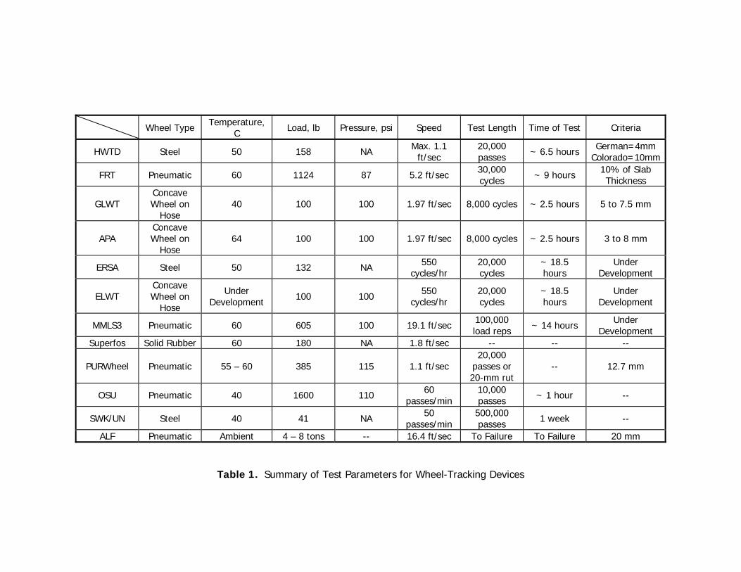
Wheel Type Temperature, C Load, lb Pressure, psi Speed Test Length Time of Test Criteria
HWTD Steel 50 158 NA Max. 1.1 ft/sec
20,000 passes ~ 6.5 hours German=4mm
Colorado=10mm
FRT Pneumatic 60 1124 87 5.2 ft/sec 30,000 cycles ~ 9 hours 10% of Slab
Thickness
GLWT Concave Wheel on
Hose 40 100 100 1.97 ft/sec 8,000 cycles ~ 2.5 hours 5 to 7.5 mm
APA Concave Wheel on
Hose 64 100 100 1.97 ft/sec 8,000 cycles ~ 2.5 hours 3 to 8 mm
ERSA Steel 50 132 NA 550 cycles/hr
20,000 cycles
~ 18.5 hours
Under Development
ELWT Concave Wheel on
Hose
Under Development 100 100 550
cycles/hr 20,000 cycles
~ 18.5 hours
Under Development
MMLS3 Pneumatic 60 605 100 19.1 ft/sec 100,000 load reps ~ 14 hours Under
Development Superfos Solid Rubber 60 180 NA 1.8 ft/sec -- -- --
PURWheel Pneumatic 55 – 60 385 115 1.1 ft/sec 20,000
passes or 20-mm rut
-- 12.7 mm
OSU Pneumatic 40 1600 110 60 passes/min
10,000 passes ~ 1 hour --
SWK/UN Steel 40 41 NA 50 passes/min
500,000 passes 1 week --
ALF Pneumatic Ambient 4 – 8 tons -- 16.4 ft/sec To Failure To Failure 20 mm
Table 1. Summary of Test Parameters for Wheel-Tracking Devices

208
State Test Temp.
Target Air Voids
Used as a Specification? Criteria
Alabama 67 4 ± 1 Yes <4.5 mm TRZ*
Arkansas 64 4 ± 1 Yes Tiered (3, 5, 8 mm) TRZ*
Delaware 67 7 ± 0.5 No <3 mm Florida 64 7 ± 0.5 No None Georgia 49 6 ± 1 Yes <5 mm Illinois 64 7 ± 1 No None Kansas <PG 7 ± 1 No To be developed
Kentucky 64 7 ± 1 No <5 mm Louisiana 64 7 ± 1 No <6 mm Michigan PG 4 – 7 No To be developed
Mississippi 64 7 ± 1 No <10 mm Missouri 64 7 ± 1 No Evaluating
New Jersey 60 4/7 ± 1 No Evaluating N. Carolina 64 7 ± 1 No Evaluating Oklahoma 64 7 ± 1 No <tiered (5, 6, 7 mm) S. Carolina 64 7 ± 1 Yes <5 mm Tennessee 64 7 ± 1 No <5-6 mm
Texas 64 7 ± 1 No Evaluating Utah 64 7 ± 1 Yes <5 mm
W. Virginia 60 7 ± 1 No <6 mm Wyoming 52/60 6 ± 1 No Evaluating
Clark Co., NV 60 6 ± 1 No <4 mm Connecticut PG 7 ± 1 No <5 mm
*TRZ = only for gradations through the restricted zone
Table 2. Summary of APA Test Criteria from 2000 APA User-Group Meeting

209
Mixture Design Information Sample Characteristics
Location Location Mix ID Sample ID
Job Number Filename Maximum # of Gyrations, Nmax Temperature
Design # of Gyrations, Ndes Load Initial # of Gyrations, Nini Channel (Right or Left)
Binder Content Wheel Type PG Grade Sample Numbers
Nominal Max. Aggregate Size Air Voids Primary Aggregate Type Gmb
Binder Specific Gravity, Gb Gmm Design Air Void Content Compaction Slope
Design Gmm Number of Gyrations Design VMA Sample Height
VMA Correction Compaction Type Design VFA Sample Shape
Fines to Asphalt Ratio Sample Width Retained Marshall Stability Sawn Faces? (Yes or No) Retained Tensile Strength VMA
Film Thickness VMAeff Design Gsb VFA Design Gse VFAeff
Percent Passing #4 Sieve Initial Consolidation* Percent Passing #8 Sieve Rutting Slope*
Percent Passing #200 Sieve Rut Depth at 10,000 Cycles* % Natural Sand Rut Depth at 20,000 Cycles* Gradation Type Stripping Slope*
Aggregate Surface Area Stripping Inflection Point (SIP)* Percent Insoluble Rut Depth at SIP*
*Response Variables Determined at Conclusion of Test
Table 3. Data Recorded for Each ERSA Wheel-Tracking Test
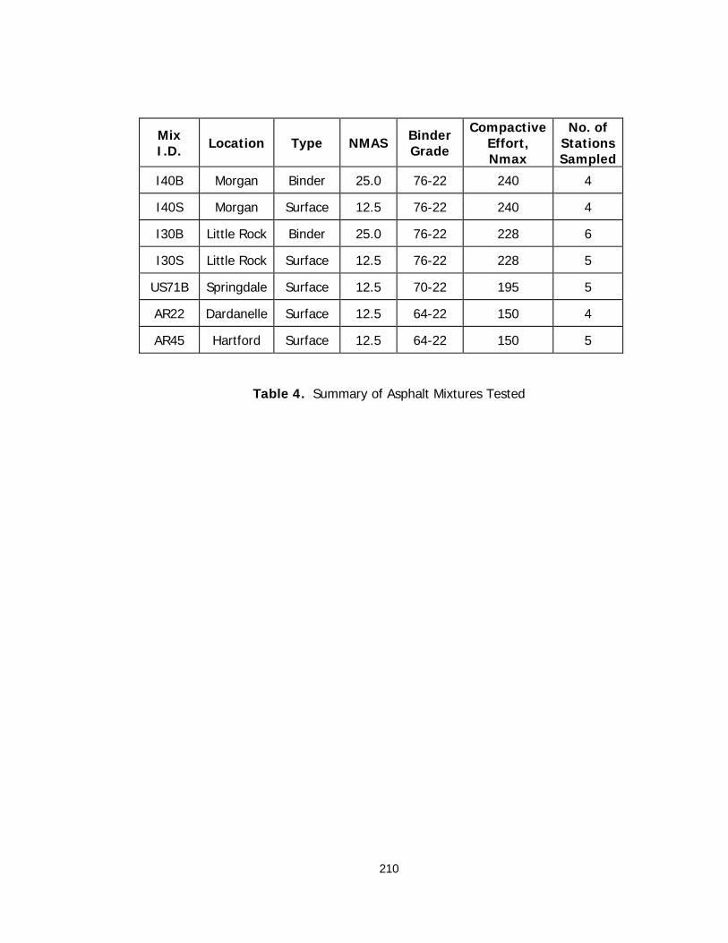
210
Table 4. Summary of Asphalt Mixtures Tested
Mix I.D. Location Type NMAS Binder
Grade
Compactive Effort, Nmax
No. of Stations Sampled
I40B Morgan Binder 25.0 76-22 240 4
I40S Morgan Surface 12.5 76-22 240 4
I30B Little Rock Binder 25.0 76-22 228 6
I30S Little Rock Surface 12.5 76-22 228 5
US71B Springdale Surface 12.5 70-22 195 5
AR22 Dardanelle Surface 12.5 64-22 150 4
AR45 Hartford Surface 12.5 64-22 150 5

211
Percent Passing this sieve… Multiply by this Factor…
Sieve Size, standard
Sieve Size, mm
Surface Area Factor, m2/kg
Surface Area Factor, ft2/lb
Maximum Maximum 0.41 2
#4 4.75 0.41 2
#8 2.36 0.82 4
#16 1.18 1.64 8
#30 0.6 2.87 14
#50 0.3 6.14 30
#100 0.15 12.29 60
#200 0.075 32.77 160
Surface Area = Sum of Products for All Sieves in Table
Table 5. Surface Area Factors for Aggregate Surface Area Calculation (3)
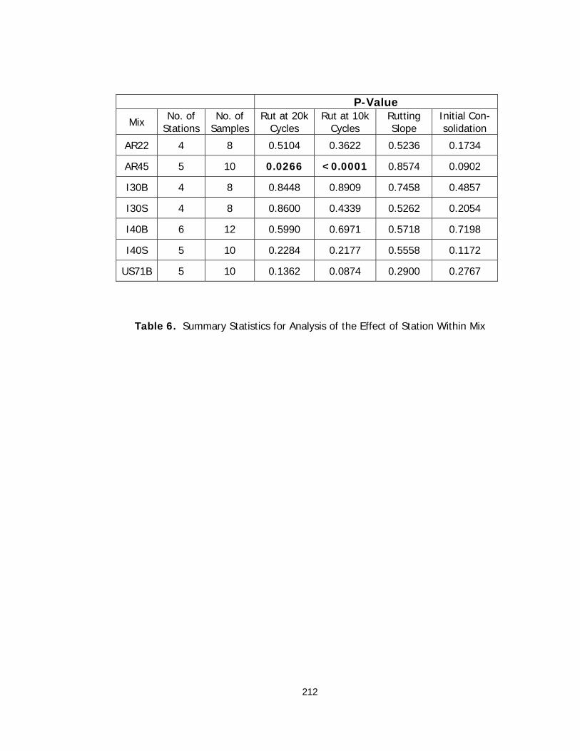
212
P-Value
Mix No. of Stations
No. of Samples
Rut at 20k Cycles
Rut at 10k Cycles
Rutting Slope
Initial Con-solidation
AR22 4 8 0.5104 0.3622 0.5236 0.1734
AR45 5 10 0.0266 <0.0001 0.8574 0.0902
I30B 4 8 0.8448 0.8909 0.7458 0.4857
I30S 4 8 0.8600 0.4339 0.5262 0.2054
I40B 6 12 0.5990 0.6971 0.5718 0.7198
I40S 5 10 0.2284 0.2177 0.5558 0.1172
US71B 5 10 0.1362 0.0874 0.2900 0.2767
Table 6. Summary Statistics for Analysis of the Effect of Station Within Mix
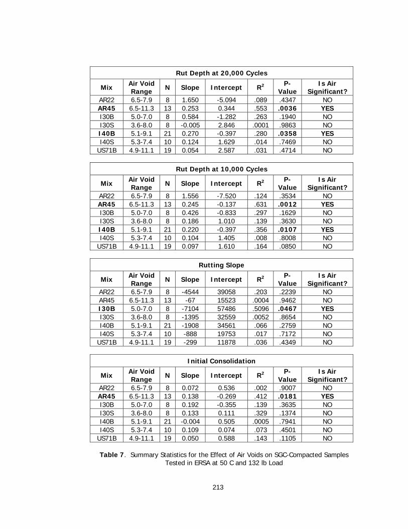
213
Rut Depth at 20,000 Cycles
Mix Air Void Range N Slope Intercept R2 P-
Value Is Air
Significant? AR22 6.5-7.9 8 1.650 -5.094 .089 .4347 NO AR45 6.5-11.3 13 0.253 0.344 .553 .0036 YES I30B 5.0-7.0 8 0.584 -1.282 .263 .1940 NO I30S 3.6-8.0 8 -0.005 2.846 .0001 .9863 NO I40B 5.1-9.1 21 0.270 -0.397 .280 .0358 YES I40S 5.3-7.4 10 0.124 1.629 .014 .7469 NO
US71B 4.9-11.1 19 0.054 2.587 .031 .4714 NO
Rut Depth at 10,000 Cycles
Mix Air Void Range N Slope Intercept R2 P-
Value Is Air
Significant? AR22 6.5-7.9 8 1.556 -7.520 .124 .3534 NO AR45 6.5-11.3 13 0.245 -0.137 .631 .0012 YES I30B 5.0-7.0 8 0.426 -0.833 .297 .1629 NO I30S 3.6-8.0 8 0.186 1.010 .139 .3630 NO I40B 5.1-9.1 21 0.220 -0.397 .356 .0107 YES I40S 5.3-7.4 10 0.104 1.405 .008 .8008 NO
US71B 4.9-11.1 19 0.097 1.610 .164 .0850 NO
Rutting Slope
Mix Air Void Range N Slope Intercept R2 P-
Value Is Air
Significant? AR22 6.5-7.9 8 -4544 39058 .203 .2239 NO AR45 6.5-11.3 13 -67 15523 .0004 .9462 NO I30B 5.0-7.0 8 -7104 57486 .5096 .0467 YES I30S 3.6-8.0 8 -1395 32559 .0052 .8654 NO I40B 5.1-9.1 21 -1908 34561 .066 .2759 NO I40S 5.3-7.4 10 -888 19753 .017 .7172 NO
US71B 4.9-11.1 19 -299 11878 .036 .4349 NO
Initial Consolidation
Mix Air Void Range N Slope Intercept R2 P-
Value Is Air
Significant? AR22 6.5-7.9 8 0.072 0.536 .002 .9007 NO AR45 6.5-11.3 13 0.138 -0.269 .412 .0181 YES I30B 5.0-7.0 8 0.192 -0.355 .139 .3635 NO I30S 3.6-8.0 8 0.133 0.111 .329 .1374 NO I40B 5.1-9.1 21 -0.004 0.505 .0005 .7941 NO I40S 5.3-7.4 10 0.109 0.074 .073 .4501 NO
US71B 4.9-11.1 19 0.050 0.588 .143 .1105 NO
Table 7. Summary Statistics for the Effect of Air Voids on SGC-Compacted Samples Tested in ERSA at 50 C and 132 lb Load

214
Stripping Slope
Mix Air Void Range N Slope Intercept R2 P-
Value Is Air
Significant? AR22 6.5-7.9 6 -1261 11170 .552 .0906 NO
Stripping Inflection Point
Mix Air Void Range N Slope Intercept R2 P-
Value Is Air
Significant? AR22 6.5-7.9 6 -3850 37150 .361 .2076 NO
Rut Depth at Stripping Inflection Point
Mix Air Void Range N Slope Intercept R2 P-
Value Is Air
Significant? AR22 6.5-7.9 6 0.237 0.737 .021 .7833 NO
Rut Depth at 20,000 Cycles
Mix Air Void Range N Slope Intercept R2 P-
Value Is Air
Significant? AR45 6.5-7.8 8 -0.357 4.672 .255 .2016 NO
Rut Depth at 10,000 Cycles
Mix Air Void Range N Slope Intercept R2 P-
Value Is Air
Significant? AR45 6.5-7.8 8 -0.201 3.020 .207 .2572 NO
Rutting Slope
Mix Air Void Range N Slope Intercept R2 P-
Value Is Air
Significant? AR45 6.5-7.8 8 2348 -1203 .109 .4244 NO
Initial Consolidation
Mix Air Void Range N Slope Intercept R2 P-
Value Is Air
Significant? AR45 6.5-7.8 8 -0.055 1.076 .034 .6618 NO
Table 7. (Cont.) Summary Statistics for the Effect of Air Voids on SGC-
Compacted Samples Tested in ERSA at 50 C and 132 lb Load
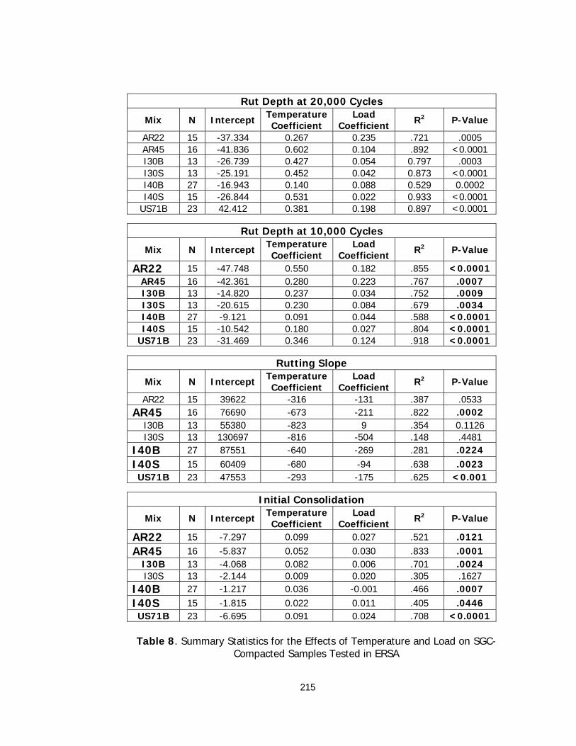
215
Rut Depth at 20,000 Cycles
Mix N Intercept Temperature Coefficient
Load Coefficient R2 P-Value
AR22 15 -37.334 0.267 0.235 .721 .0005 AR45 16 -41.836 0.602 0.104 .892 <0.0001 I30B 13 -26.739 0.427 0.054 0.797 .0003 I30S 13 -25.191 0.452 0.042 0.873 <0.0001 I40B 27 -16.943 0.140 0.088 0.529 0.0002 I40S 15 -26.844 0.531 0.022 0.933 <0.0001
US71B 23 42.412 0.381 0.198 0.897 <0.0001
Rut Depth at 10,000 Cycles
Mix N Intercept Temperature Coefficient
Load Coefficient R2 P-Value
AR22 15 -47.748 0.550 0.182 .855 <0.0001AR45 16 -42.361 0.280 0.223 .767 .0007 I30B 13 -14.820 0.237 0.034 .752 .0009 I30S 13 -20.615 0.230 0.084 .679 .0034 I40B 27 -9.121 0.091 0.044 .588 <0.0001I40S 15 -10.542 0.180 0.027 .804 <0.0001
US71B 23 -31.469 0.346 0.124 .918 <0.0001
Rutting Slope
Mix N Intercept Temperature Coefficient
Load Coefficient R2 P-Value
AR22 15 39622 -316 -131 .387 .0533 AR45 16 76690 -673 -211 .822 .0002
I30B 13 55380 -823 9 .354 0.1126 I30S 13 130697 -816 -504 .148 .4481
I40B 27 87551 -640 -269 .281 .0224 I40S 15 60409 -680 -94 .638 .0023 US71B 23 47553 -293 -175 .625 <0.001
Initial Consolidation
Mix N Intercept Temperature Coefficient
Load Coefficient R2 P-Value
AR22 15 -7.297 0.099 0.027 .521 .0121 AR45 16 -5.837 0.052 0.030 .833 .0001
I30B 13 -4.068 0.082 0.006 .701 .0024 I30S 13 -2.144 0.009 0.020 .305 .1627
I40B 27 -1.217 0.036 -0.001 .466 .0007 I40S 15 -1.815 0.022 0.011 .405 .0446 US71B 23 -6.695 0.091 0.024 .708 <0.0001
Table 8. Summary Statistics for the Effects of Temperature and Load on SGC-
Compacted Samples Tested in ERSA

216
Stripping Slope
Mix N Intercept Temperature Coefficient
Load Coefficient R2 P-Value
AR22 12 13048 -117 -37 .766 .0014 AR45 4 .172 .5854
I30B 1 NA NA I30S 3 .0004 .9877
I40B 0 NA NA
I40S 3 1.00 .0027 US71B 4
Model is not full rank. No parameter estimates available.
.468 .3160
Stripping Inflection Point
Mix N Intercept Temperature Coefficient
Load Coefficient R2 P-Value
AR22 12 52000 -546 109 .736 .0025 AR45 4 .266 .4846
I30B 1 NA NA I30S 3 .470 .5193
I40B 0 NA NA
I40S 3 .168 .7313 US71B 4
Model is not full rank. No parameter estimates available.
.027 .8365
Rut Depth at Stripping Inflection Point
Mix N Intercept Temperature Coefficient
Load Coefficient R2 P-Value
AR22 12 -4.602 0.012 0.053 .125 .5481
AR45 4 .035 .8136 I30B 1 NA NA I30S 3 .296 .6337
I40B 0 NA NA
I40S 3 .515 .4903 US71B 4
Model is not full rank. No parameter estimates available.
.178 .5787
Table 8. (Cont.) Summary Statistics for the Effects of Temperature and Load on SGC-Compacted Samples Tested in ERSA

217
Field Compacted Samples
P-Values
Mix N Rut at 20k Cycles
Rut at 10k Cycles
Rutting Slope
Initial Consolidation
AR22 11 0.4167 0.5576 0.1356 .0352 AR45 21 0.6799 0.0032 0.0211 0.1449 I30B 0 - - - - I30S 30 0.5059 0.7447 0.7011 0.7011 I40B 0 - - - - I40S 18 0.1526 0.1584 0.1090 0.3636
US71B 0 - - - -
Field Compacted Samples P-Values
Mix N Stripping Slope Stripping Inflection Point
Rut Depth at SIP
AR22 10 0.0708 0.2292 0.3077 AR45 20 0.9530 0.0021 0.0312 I30B 0 - - - I30S 14 0.3804 0.2814 0.7911 I40B 0 - - - I40S 0 - - -
US71B 0 - - -
Lab Compacted Samples P-Values
Mix N Rut at 20k Cycles
Rut at 10k Cycles
Rutting Slope
Initial Consolidation
AR22 0 - - - - AR45 0 - - - - I30B 0 - - - - I30S 13 0.3588 0.3471 0.3453 0.9149 0I40B 0 - - - - I40S 0 - - - -
US71B 0 - - - -
Table 9. Summary Statistics for the Effect of Sample Shape on Samples Tested in ERSA at 50 C and 132 lb Load
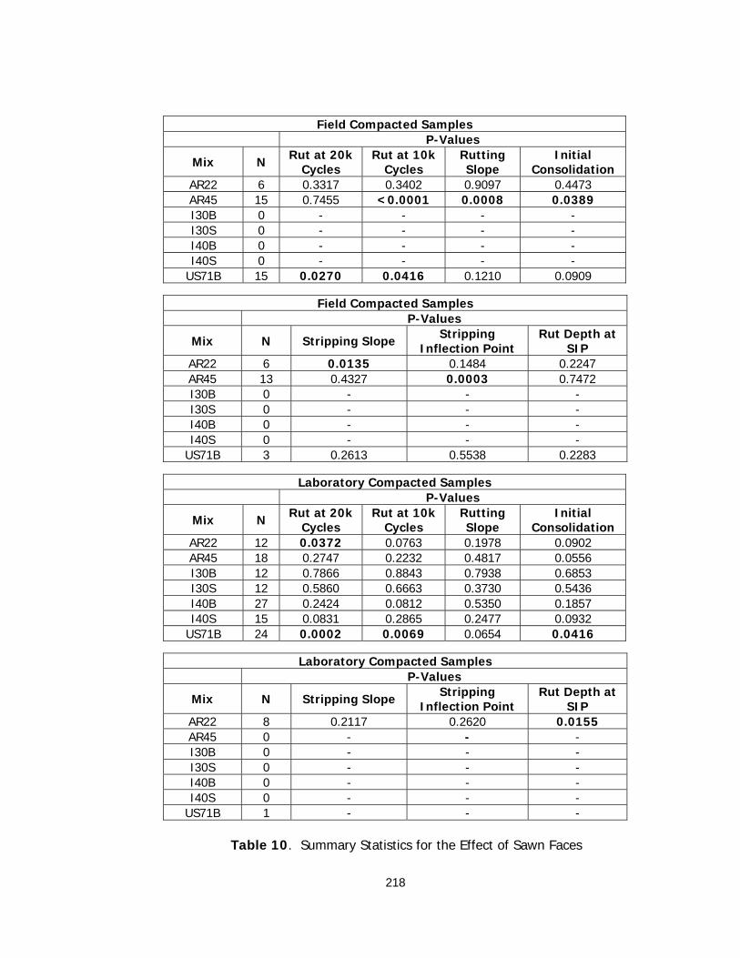
218
Field Compacted Samples
P-Values
Mix N Rut at 20k Cycles
Rut at 10k Cycles
Rutting Slope
Initial Consolidation
AR22 6 0.3317 0.3402 0.9097 0.4473 AR45 15 0.7455 <0.0001 0.0008 0.0389 I30B 0 - - - - I30S 0 - - - - I40B 0 - - - - I40S 0 - - - -
US71B 15 0.0270 0.0416 0.1210 0.0909
Field Compacted Samples P-Values
Mix N Stripping Slope Stripping Inflection Point
Rut Depth at SIP
AR22 6 0.0135 0.1484 0.2247 AR45 13 0.4327 0.0003 0.7472 I30B 0 - - - I30S 0 - - - I40B 0 - - - I40S 0 - - -
US71B 3 0.2613 0.5538 0.2283
Laboratory Compacted Samples P-Values
Mix N Rut at 20k Cycles
Rut at 10k Cycles
Rutting Slope
Initial Consolidation
AR22 12 0.0372 0.0763 0.1978 0.0902 AR45 18 0.2747 0.2232 0.4817 0.0556 I30B 12 0.7866 0.8843 0.7938 0.6853 I30S 12 0.5860 0.6663 0.3730 0.5436 I40B 27 0.2424 0.0812 0.5350 0.1857 I40S 15 0.0831 0.2865 0.2477 0.0932
US71B 24 0.0002 0.0069 0.0654 0.0416
Laboratory Compacted Samples P-Values
Mix N Stripping Slope Stripping Inflection Point
Rut Depth at SIP
AR22 8 0.2117 0.2620 0.0155 AR45 0 - - - I30B 0 - - - I30S 0 - - - I40B 0 - - - I40S 0 - - -
US71B 1 - - -
Table 10. Summary Statistics for the Effect of Sawn Faces

219
P-Values
Mix N Rut at
20k Cycles
Rut at 10k
Cycles
Rutting Slope
Initial Consolidation
AR22 12 0.4397 0.5160 0.6353 0.0450 AR45 11 0.4846 0.5507 0.9518 0.8336 I30B Not Tested
I30S - Lab 5 0.7715 0.8617 0.5165 0.4916 I40B Not Tested I40S Not Tested
US71B Not Tested
P-Values
Mix N Stripping Slope Stripping Inflection Point
Rut Depth at SIP
AR22 11 0.6927 0.7295 0.6801 AR45 11 0.2757 0.7210 0.6478 I30B Not Tested
I30S - Lab Did Not Strip I40B Not Tested I40S Not Tested
US71B Not Tested
Table 11. Summary Statistics for the Effect of Slab Width

220
Rut Depth at 20,000 Cycles
Mix N P-Value Mean of Field Samples (mm)
Mean of Lab Samples (mm)
AR22 25 <0.0001 13.09 6.56 AR45 34 <0.0001 10.95 2.49 I30B No Field Samples Tested I30S 43 <0.0001 7.55 3.11 I40B No Field Samples Tested I40S 28 0.0021 4.76 2.41
US71B 29 <0.0001 5.40 3.00
Rut Depth at 10,000 Cycles
Mix N P-Value Mean of Field Samples (mm)
Mean of Lab Samples (mm)
AR22 25 <0.0001 12.83 3.48 AR45 34 <0.0001 5.86 1.95 I30B No Field Samples Tested I30S 43 <0.0001 4.21 2.27 I40B No Field Samples Tested I40S 28 0.0103 3.27 2.06
US71B 29 0.0002 3.44 2.35
Rutting Slope
Mix N P-Value Mean of Field Samples (cyc/mm)
Mean of Lab Samples (cyc/mm)
AR22 25 <0.0001 717 6949 AR45 34 <0.0001 2612 14954 I30B No Field Samples Tested I30S 43 0.1009 7809 18977 I40B No Field Samples Tested I40S 28 0.0021 7735 14177
US71B 29 0.0056 6246 9605
Initial Consolidation
Mix N P-Value Mean of Field Samples (mm)
Mean of Lab Samples (mm)
AR22 25 0.0002 2.30 1.05 AR45 34 0.0799 1.13 0.90 I30B No Field Samples Tested I30S 43 0.0022 1.26 0.88 I40B No Field Samples Tested I40S 28 0.0083 1.14 0.76
US71B 29 0.0282 1.25 0.97
Table 12. Summary Statistics for the Effect of Compaction Type on Samples Tested in ERSA at 50 C and 132 lb Load

221
Stripping Slope
Mix N P-Value Mean of Field Samples (cyc/mm)
Mean of Lab Samples (cyc/mm)
AR22 21 <0.0001 321 2490 AR45 Lab Samples Did Not Strip I30B No Field Samples Tested I30S Lab Samples Did Not Strip I40B No Field Samples Tested I40S Samples Did Not Strip
US71B Lab Samples Did Not Strip
Stripping Inflection Point
Mix N P-Value Mean of Field Samples (cyc)
Mean of Lab Samples (cyc)
AR22 21 <0.0001 3067 10650 AR45 Lab Samples Did Not Strip I30B No Field Samples Tested I30S Lab Samples Did Not Strip I40B No Field Samples Tested I40S Samples Did Not Strip
US71B Lab Samples Did Not Strip
Rut Depth at Stripping Inflection Point
Mix N P-Value Mean of Field Samples (mm)
Mean of Lab Samples (mm)
AR22 21 <0.0001 5.86 2.37 AR45 Lab Samples Did Not Strip I30B No Field Samples Tested I30S Lab Samples Did Not Strip I40B No Field Samples Tested I40S Samples Did Not Strip
US71B Lab Samples Did Not Strip
Table 12. (Cont.) Summary Statistics for the Effect of Compaction Type on Samples Tested in ERSA at 50 C and 132 lb Load

222
Automatic APA Rut Depth Measurements at 8,000 Cycles
Mix Air Void Range N Slope Intercept R2 P-
Value Is Air
Significant? AR22 6.4-8.2 12 -0.309 5.383 .031 .5834 NO AR45 7.1-8.4 15 0.303 -0.201 .101 .2483 NO I30B 5.9-7.2 12 0.027 1.332 .002 .9007 NO I30S 6.2-7.9 8 -0.226 3.228 .158 .3289 NO I40B 5.2-8.1 18 -0.007 .962 .001 .8862 NO I40S 5.7-8.1 15 -0.076 1.589 .001 .9204 NO
US71B 6.2-8.2 15 -0.147 3.051 .038 .4854 NO
Manual APA Rut Depth Measurements at 8,000 Cycles
Mix Air Void Range N Slope Intercept R2 P-
Value Is Air
Significant? AR22 6.4-8.2 12 -0.366 6.541 .085 .3595 NO AR45 7.1-8.4 15 0.713 -2.440 .106 .2354 NO I30B 5.9-7.2 12 -0.287 3.923 .038 .5442 NO I30S 6.2-7.9 8 0.017 1.773 .001 .9614 NO I40B 5.2-8.1 18 0.049 0.823 .017 .6086 NO I40S 5.7-8.1 15 0.225 0.198 .074 .3269 NO
US71B 6.2-8.2 15 0.021 2.287 .001 .9099 NO
Table 13. Summary Statistics for the Effect of Air Voids of SGC-Compacted Samples Tested in the APA at 50 C

223
Automatic Measurement of Rut Depth in APA Average Rut Depth
(mm) Average Air Void
Content (%) Mix N P-Value Dry Wet Dry Wet
AR22 13 .3624 3.985 3.090 8.8 7.4 AR45 16 .3305 2.483 2.096 6.4 7.6 I30B 13 .0004 2.885 1.508 8.3 6.5 I30s 13 .5217 1.899 1.638 6.8 7.0
I40B 19 <0.0001 1.913 0.913 9.5 6.9 I40S 16 .3987 1.874 1.475 6.0 6.8
US71B 16 .0051 3.349 1.970 8.6 7.4
Manual Measurement of Rut Depth in APA Average Rut Depth
(mm) Average Air Void
Content (%) Mix N P-Value Dry Wet Dry Wet
AR22 13 .0649 5.213 3.823 8.8 7.4 AR45 16 .9826 2.985 2.965 6.4 7.6 I30B 13 .0370 3.508 2.064 8.3 6.5 I30s 13 .5377 2.268 1.896 6.8 7.0
I40B 19 <0.0001 2.893 1.158 9.5 6.9 I40S 16 .5079 2.180 1.742 6.0 6.8
US71B 16 .0002 4.230 2.442 8.6 7.4
Table 14. Summary Statistics for the Effect of Wet vs. Dry Testing on SGC-Compacted Samples Tested in the APA at 50 C

224
Mix N Mean Rut Depth for Automatic
Mean Rut Depth for Manual
P-Value
Is Method Significant?
AR22 24 3.090 3.823 .0327 YES AR45 30 2.096 2.965 .0012 YES I30B 24 1.508 2.064 .0067 YES I30S 24 1.638 1.896 .2837 NO
I40B 36 0.913 1.158 .0081 YES I40S 30 1.475 1.742 .1877 NO
US71B 30 1.970 2.442 .0019 YES
Table 15. Summary Statistics for the Effect of Automatic vs. Manual Measurement Method on SGC-Compacted Samples Tested Wet in APA at 50 C

225
Automatic Measurement Method
Mix N Mean Rut Depth for
50 C
Mean Rut Depth for
64 C P-Value
Is Temperature Significant?
AR22 24 3.090 5.907 <0.0001 YES AR45 30 2.096 4.006 <0.0001 YES I30B 24 1.508 2.884 <0.0001 YES I30S 24 1.638 3.132 <0.0001 YES I40B 36 0.913 1.746 <0.0001 YES I40S 30 1.475 2.820 <0.0001 YES
US71B 30 1.970 3.766 <0.0001 YES
Manual Measurement Method
Mix N Mean Rut Depth for
50 C
Mean Rut Depth for
64 C P-Value
Is Temperature Significant?
AR22 24 3.823 7.309 <0.0001 YES AR45 30 2.965 5.669 <0.0001 YES I30B 24 2.064 3.945 <0.0001 YES I30S 24 1.896 3.624 0.0009 YES I40B 36 1.158 2.214 <0.0001 YES I40S 30 1.742 3.330 <0.0001 YES
US71B 30 2.442 4.668 <0.0001 YES
Table 16. Summary Statistics for the Effect of Temperature (based on TEM) on SGC-Compacted Samples Tested Wet in the APA.

226
Field Compacted Samples
P-Values
Mix N Rut at 20k Cycles
Rut at 10k Cycles
Rutting Slope
Initial Consolidation
AR22 6 .2287 .1642 .6670 .1838 AR45 16 .1830 .1253 .8535 .0866 I30B 0 - - - - I30S 0 - - - - I40B 0 - - - - I40S 0 - - - -
US71B 0 - - - -
Table 17. Summary Statistics for the Effect of Sample Shape on Samples Tested in the ELWT at 50 C
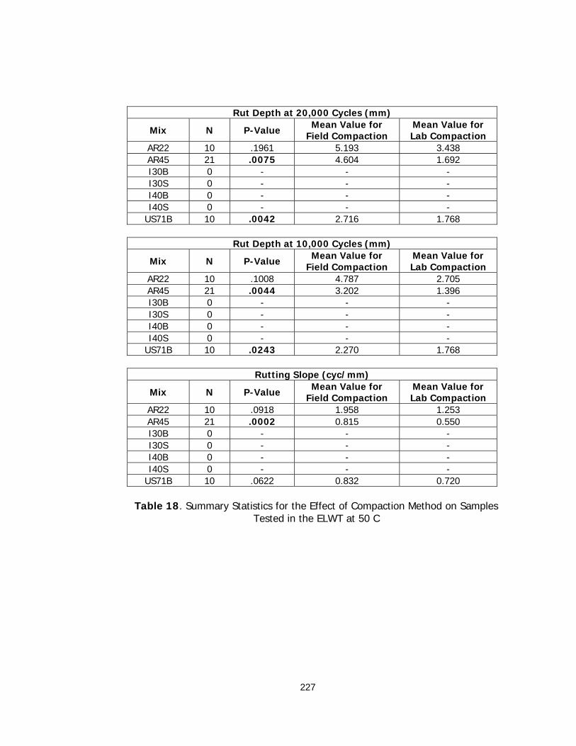
227
Rut Depth at 20,000 Cycles (mm)
Mix N P-Value Mean Value for Field Compaction
Mean Value for Lab Compaction
AR22 10 .1961 5.193 3.438 AR45 21 .0075 4.604 1.692 I30B 0 - - - I30S 0 - - - I40B 0 - - - I40S 0 - - -
US71B 10 .0042 2.716 1.768
Rut Depth at 10,000 Cycles (mm)
Mix N P-Value Mean Value for Field Compaction
Mean Value for Lab Compaction
AR22 10 .1008 4.787 2.705 AR45 21 .0044 3.202 1.396 I30B 0 - - - I30S 0 - - - I40B 0 - - - I40S 0 - - -
US71B 10 .0243 2.270 1.768
Rutting Slope (cyc/mm)
Mix N P-Value Mean Value for Field Compaction
Mean Value for Lab Compaction
AR22 10 .0918 1.958 1.253 AR45 21 .0002 0.815 0.550 I30B 0 - - - I30S 0 - - - I40B 0 - - - I40S 0 - - -
US71B 10 .0622 0.832 0.720
Table 18. Summary Statistics for the Effect of Compaction Method on Samples Tested in the ELWT at 50 C
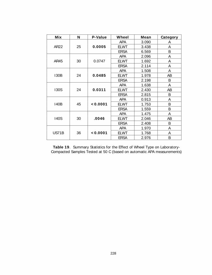
228
Mix N P-Value Wheel Mean Category
APA 3.090 A ELWT 3.438 A AR22 25 0.0005
ERSA 6.569 B APA 2.096 A
ELWT 1.692 A AR45 30 0.0747 ERSA 2.114 A APA 1.508 A
ELWT 1.978 AB I30B 24 0.0485 ERSA 2.198 B APA 1.638 A
ELWT 2.430 AB I30S 24 0.0311 ERSA 2.815 B APA 0.913 A
ELWT 1.753 B I40B 45 <0.0001 ERSA 1.559 B APA 1.475 A
ELWT 2.046 AB I40S 30 .0046 ERSA 2.408 B APA 1.970 A
ELWT 1.768 A US71B 36 <0.0001 ERSA 2.976 B
Table 19. Summary Statistics for the Effect of Wheel Type on Laboratory-
Compacted Samples Tested at 50 C (based on automatic APA measurements)

229
Mix N P-Value Wheel Mean Category
APA 3.823 A ELWT 3.438 A AR22 25 0.0023 ERSA 6.569 B APA 2.965 A
ELWT 1.692 B AR45 30 0.0015 ERSA 2.114 B APA 2.064 A
ELWT 1.978 A I30B 24 0.8567 ERSA 2.198 A APA 1.896 A
ELWT 2.430 A I30S 24 0.1270 ERSA 2.815 A APA 1.158 A
ELWT 1.753 B I40B 45 0.0155 ERSA 1.559 B APA 1.742 A
ELWT 2.046 A I40S 30 0.0955 ERSA 2.408 A APA 2.442 A
ELWT 1.768 B US71B 36 <0.0001 ERSA 2.976 C
Table 20. Summary Statistics for the Effect of Wheel Type on Laboratory-Compacted Samples Tested at 50 C (based on manual APA measurements)

230
Mix N P-Value Wheel Mean Category
APA 5.907 A ELWT 3.438 A AR22 25 0.0551
*marginal ERSA 6.569 A APA 4.006 A
ELWT 1.692 B AR45 30 <0.0001 ERSA 2.114 B APA 2.884 A
ELWT 1.978 B I30B 24 0.0323 ERSA 2.198 B APA 3.132 A
ELWT 2.430 A I30S 24 0.4507 ERSA 2.815 A APA 1.746 A
ELWT 1.753 A I40B 45 0.4553 ERSA 1.559 A APA 2.800 A
ELWT 2.046 A I40S 30 0.1708 ERSA 2.408 A APA 3.766 A
ELWT 1.768 B US71B 36 <0.0001 ERSA 2.976 C
Table 21. Summary Statistics for the Effect of Wheel Type on Laboratory-
Compacted Samples - ERSA and ELWT Samples Tested at 50 C and APA Samples at 64 C (based on TEM and automatic APA measurements)
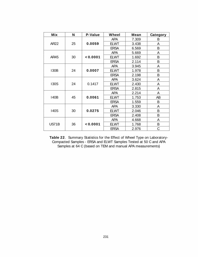
231
Mix N P-Value Wheel Mean Category
APA 7.309 B ELWT 3.438 A AR22 25 0.0059 ERSA 6.569 B APA 5.669 A
ELWT 1.692 B AR45 30 <0.0001 ERSA 2.114 B APA 3.945 A
ELWT 1.978 B I30B 24 0.0007 ERSA 2.198 B APA 3.624 A
ELWT 2.430 A I30S 24 0.1417 ERSA 2.815 A APA 2.214 A
ELWT 1.753 AB I40B 45 0.0061 ERSA 1.559 B APA 3.330 A
ELWT 2.046 B I40S 30 0.0275 ERSA 2.408 B APA 4.668 A
ELWT 1.768 B US71B 36 <0.0001 ERSA 2.976 C
Table 22. Summary Statistics for the Effect of Wheel Type on Laboratory-
Compacted Samples - ERSA and ELWT Samples Tested at 50 C and APA Samples at 64 C (based on TEM and manual APA measurements)
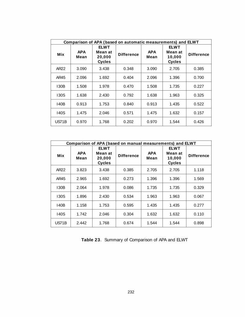
232
Comparison of APA (based on automatic measurements) and ELWT
Mix APA Mean
ELWT Mean at 20,000 Cycles
Difference APA Mean
ELWT Mean at 10,000 Cycles
Difference
AR22 3.090 3.438 0.348 3.090 2.705 0.385
AR45 2.096 1.692 0.404 2.096 1.396 0.700
I30B 1.508 1.978 0.470 1.508 1.735 0.227
I30S 1.638 2.430 0.792 1.638 1.963 0.325
I40B 0.913 1.753 0.840 0.913 1.435 0.522
I40S 1.475 2.046 0.571 1.475 1.632 0.157
US71B 0.970 1.768 0.202 0.970 1.544 0.426
Comparison of APA (based on manual measurements) and ELWT
Mix APA Mean
ELWT Mean at 20,000 Cycles
Difference APA Mean
ELWT Mean at 10,000 Cycles
Difference
AR22 3.823 3.438 0.385 2.705 2.705 1.118
AR45 2.965 1.692 0.273 1.396 1.396 1.569
I30B 2.064 1.978 0.086 1.735 1.735 0.329
I30S 1.896 2.430 0.534 1.963 1.963 0.067
I40B 1.158 1.753 0.595 1.435 1.435 0.277
I40S 1.742 2.046 0.304 1.632 1.632 0.110
US71B 2.442 1.768 0.674 1.544 1.544 0.898
Table 23. Summary of Comparison of APA and ELWT
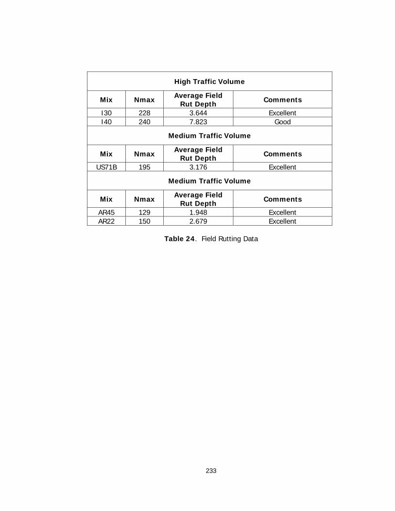
233
High Traffic Volume
Mix Nmax Average Field Rut Depth Comments
I30 228 3.644 Excellent I40 240 7.823 Good
Medium Traffic Volume
Mix Nmax Average Field Rut Depth Comments
US71B 195 3.176 Excellent
Medium Traffic Volume
Mix Nmax Average Field Rut Depth Comments
AR45 129 1.948 Excellent AR22 150 2.679 Excellent
Table 24. Field Rutting Data

234
ERSA Lab Cores – 50 C – 132 lb Load – Not Sawn
Mix N Mean Standard Deviation Rank
I40B 21 1.559 0.610 A AR45 10 2.114 0.313 AB I30B 8 2.198 0.945 AB I40S 10 2.408 0.712 B I30S 8 2.815 1.157 B
US71B 16 2.976 0.618 B AR22 8 6.569 2.620 C
ERSA Lab Cores – 50 C – 132 lb Load – Sawn
Mix N Mean Standard Deviation Rank
I40B 6 1.880 0.4307 A I30B 4 2.060 0.302 A AR45 5 3.016 1.401 A I30S 4 3.313 1.955 AB I40S 5 3.374 1.315 AB
US71B 5 4.982 1.617 B AR22 4 10.333 0.435 C
ERSA Lab Cores – 50 C – 160 lb Load – Not Sawn
Mix N Mean Standard Deviation Rank
I30B 2 1.785 0.134 A AR45 2 3.910 NA AB I40B 2 4.445 2.906 AB I30S 2 4.475 0.742 AB I40S 1 4.580 NA AB
US71B 2 7.235 0.262 B AR22 2 15.540 0.552 C
ERSA Lab Cores – 64 C – 132 lb Load – Not Sawn
Mix N Mean Standard Deviation Rank
I40B 2 3.940 0.127 A I30B 1 4.700 NA AB
US71B 2 7.015 0.686 ABC AR45 2 9.925 3.570 BCD I30S 2 10.030 NA BCD I40S 2 10.700 1.131 CD AR22 2 12.700 0.354 D
Table 25. ERSA Rankings Relative to Rut Depth at 20,000 Cycles
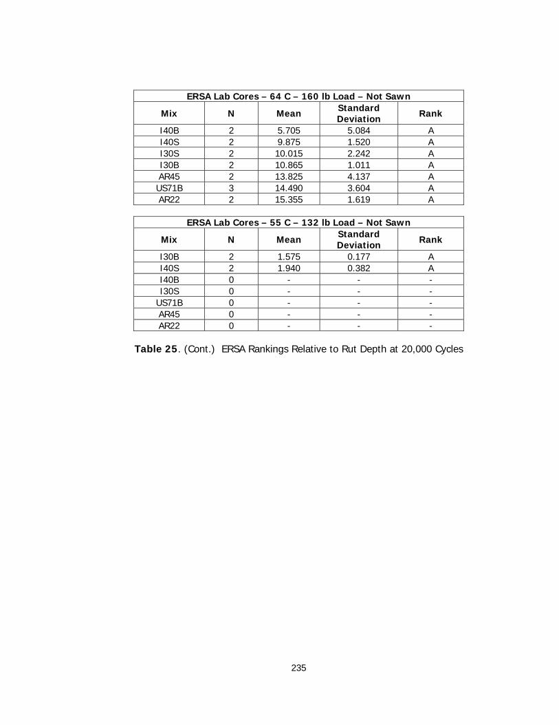
235
ERSA Lab Cores – 64 C – 160 lb Load – Not Sawn
Mix N Mean Standard Deviation Rank
I40B 2 5.705 5.084 A I40S 2 9.875 1.520 A I30S 2 10.015 2.242 A I30B 2 10.865 1.011 A AR45 2 13.825 4.137 A US71B 3 14.490 3.604 A AR22 2 15.355 1.619 A
ERSA Lab Cores – 55 C – 132 lb Load – Not Sawn
Mix N Mean Standard Deviation Rank
I30B 2 1.575 0.177 A I40S 2 1.940 0.382 A I40B 0 - - - I30S 0 - - -
US71B 0 - - - AR45 0 - - - AR22 0 - - -
Table 25. (Cont.) ERSA Rankings Relative to Rut Depth at 20,000 Cycles

236
ERSA Lab Cores – 50 C – 132 lb Load – Not Sawn
Mix N Mean Standard Deviation Rank
I40B 21 1.196 0.442 A AR45 10 1.575 0.196 AB I30B 8 1.706 0.649 AB I40S 10 2.060 0.764 B I30S 8 2.094 0.797 B
US71B 16 2.299 0.456 B AR22 8 3.479 2.100 C
ERSA Lab Cores – 50 C – 132 lb Load – Sawn
Mix N Mean Standard Deviation Rank
I40B 6 1.573 0.471 A I30B 4 1.653 0.413 AB I30S 4 2.375 1.442 AB AR45 5 2.480 1.261 AB I40S 5 2.552 0.900 AB
US71B 5 3.092 0.679 B AR22 4 6.233 2.053 C
ERSA Lab Cores – 50 C – 160 lb Load – Not Sawn
Mix N Mean Standard Deviation Rank
I30B 2 1.730 0.042 A I40B 2 2.640 0.820 A I40S 1 2.910 NA A AR45 2 3.200 NA A I30S 2 3.800 NA A
US71B 2 4.660 0.085 A AR22 2 10.060 2.644 B
ERSA Lab Cores – 64 C – 132 lb Load – Not Sawn
Mix N Mean Standard Deviation Rank
I40B 2 2.670 0.311 A AR45 2 2.930 2.410 A I30B 1 3.340 NA A I30S 1 4.160 NA A I40S 2 4.630 0.665 A
US71B 2 6.040 2.065 A AR22 2 12.680 0.318 B
Table 26. ERSA Rankings Relative to Rut Depth at 10,000 Cycles
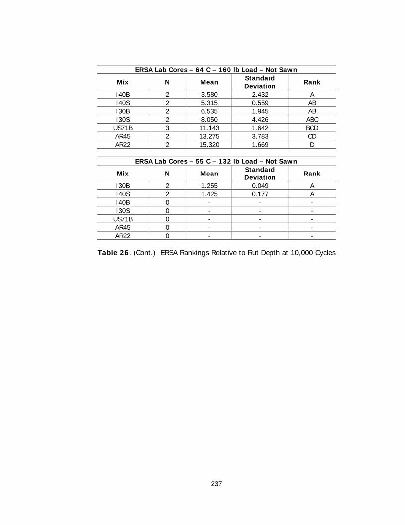
237
ERSA Lab Cores – 64 C – 160 lb Load – Not Sawn
Mix N Mean Standard Deviation Rank
I40B 2 3.580 2.432 A I40S 2 5.315 0.559 AB I30B 2 6.535 1.945 AB I30S 2 8.050 4.426 ABC
US71B 3 11.143 1.642 BCD AR45 2 13.275 3.783 CD AR22 2 15.320 1.669 D
ERSA Lab Cores – 55 C – 132 lb Load – Not Sawn
Mix N Mean Standard Deviation Rank
I30B 2 1.255 0.049 A I40S 2 1.425 0.177 A I40B 0 - - - I30S 0 - - -
US71B 0 - - - AR45 0 - - - AR22 0 - - -
Table 26. (Cont.) ERSA Rankings Relative to Rut Depth at 10,000 Cycles

238
ERSA Lab Cores – 50 C – 132 lb Load – Not Sawn
Mix N Mean Standard Deviation Rank
I30S 8 24414 31018 A I40B 21 20598 8639 A AR45 10 15642 3151 AB I30B 8 15130 8257 AB I40S 10 14177 4542 AB
US71B 16 9951 3002 B AR22 8 6949 4787 B
ERSA Lab Cores – 50 C – 132 lb Load – Sawn
Mix N Mean Standard Deviation Rank
I40B 6 18151 7164 A AR45 5 16955 3154 AB I30B 4 13926 4441 AB I40S 5 10713 6505 B I30S 4 9539 4045 BC
US71B 5 6868 2227 C AR22 4 2979 1234 C
ERSA Lab Cores – 50 C – 160 lb Load – Not Sawn
Mix N Mean Standard Deviation Rank
I30B 2 16911 7501 A I40S 1 9278 NA A I40B 2 7372 1123 A AR45 2 5917 NA A I30S 2 5146 2799 A
US71B 2 3965 281 A AR22 2 1259 324 A
ERSA Lab Cores – 64 C – 132 lb Load – Not Sawn
Mix N Mean Standard Deviation Rank
I30B 1 6363 NA A I40B 2 5932 573 A
US71B 2 4761 1022 AB AR45 2 4098 1403 AB I30S 1 3713 NA AB I40S 2 3420 303 B AR22 2 502 235 C
Table 27. ERSA Rankings Relative to Rutting Slope

239
ERSA Lab Cores – 64 C – 160 lb Load – Not Sawn
Mix N Mean Standard Deviation Rank
I40B 2 8780 8620 A I30B 2 2948 1277 A I40S 2 2841 392 A I30S 2 1976 1246 A AR45 3 1593 646 A US71B 2 1479 299 A AR22 2 160 25 A
ERSA Lab Cores – 55 C – 132 lb Load – Not Sawn
Mix N Mean Standard Deviation Rank
I30B 2 20471 3972 A I40S 2 16363 3876 A I40B 0 - - - I30S 0 - - -
US71B 0 - - - AR45 0 - - - AR22 0 - - -
Table 27. (Cont.) ERSA Rankings Relative to Rutting Slope

240
ERSA Lab Cores – 50 C – 132 lb Load – Not Sawn
Mix N Mean Standard Deviation Rank
I40B 21 0.479 0.193 A AR45 10 0.683 0.132 AB I40S 10 0.761 0.273 BC I30B 8 0.791 0.428 BC I30S 8 0.886 0.371 BC
US71B 16 0.966 0.266 BC AR22 8 1.046 0.699 C
ERSA Lab Cores – 50 C – 132 lb Load – Sawn
Mix N Mean Standard Deviation Rank
I40B 6 0.595 0.142 A I30B 4 0.698 0.144 A I30S 4 0.738 0.421 A I40S 5 1.014 0.210 AB
US71B 5 1.222 0.169 ABC AR45 5 1.738 1.387 BC AR22 4 2.070 1.183 C
ERSA Lab Cores – 50 C – 160 lb Load – Not Sawn
Mix N Mean Standard Deviation Rank
I40B 2 0.340 0.283 A I30B 2 0.925 0.191 A I40S 1 1.480 NA A AR45 2 1.520 NA A I30S 2 1.780 0.721 A
US71B 2 1.885 0.078 A AR22 2 2.290 0.849 A
ERSA Lab Cores – 64 C – 132 lb Load – Not Sawn
Mix N Mean Standard Deviation Rank
I40B 2 0.875 0.064 A I40S 2 1.290 0.071 A AR45 2 1.415 0.191 A I30S 1 1.600 NA AB I30B 1 1.890 NA ABC
US71B 2 2.495 0.841 BC AR22 2 2.930 0.198 C
Table 28. ERSA Rankings Relative to Initial Consolidation

241
ERSA Lab Cores – 64 C – 160 lb Load – Not Sawn
Mix N Mean Standard Deviation Rank
I40B 2 1.030 0.339 A I40S 2 1.245 0.417 A I30B 2 1.375 0.601 A I30S 2 2.115 0.417 A AR45 2 2.240 0.849 A US71B 3 2.783 1.144 A AR22 2 2.850 1.626 A
ERSA Lab Cores – 55 C – 132 lb Load – Not Sawn
Mix N Mean Standard Deviation Rank
I30B 2 0.555 0.007 A I40S 2 0.620 0.057 A I40B 0 - - - I30S 0 - - -
US71B 0 - - - AR45 0 - - - AR22 0 - - -
Table 28. (Cont.) ERSA Rankings Relative to Initial Consolidation

242
ERSA Lab Cores – 50 C – 132 lb Load – Not Sawn
Mix N Mean Standard Deviation Rank
I30B 0 - - DNS I30S 0 - - DNS I40B 0 - - DNS I40S 0 - - DNS AR45 0 - - DNS US71B 0 - - DNS AR22 8 2490 674 A
ERSA Lab Cores – 50 C – 132 lb Load – Sawn
Mix N Mean Standard Deviation Rank
I30B 0 - - DNS I30S 0 - - DNS I40B 0 - - DNS I40S 0 - - DNS AR45 0 - - DNS AR22 4 1787 67 A US71B 1 746 NA B
ERSA Lab Cores – 50 C – 160 lb Load – Not Sawn
Mix N Mean Standard Deviation Rank
I30B 0 - - DNS I30S 0 - - DNS I40B 0 - - DNS I40S 0 - - DNS AR45 0 - - DNS US71B 0 - - DNS AR22 2 851 287 A
ERSA Lab Cores – 64 C – 132 lb Load – Not Sawn
Mix N Mean Standard Deviation Rank
I30B 0 - - DNS I40B 0 - - DNS I30S 1 1309 NA A I40S 2 1279 2 A
US71B 1 841 NA B AR45 2 510 117 C AR22 2 247 25 D
Table 29. ERSA Rankings Relative to Stripping Slope
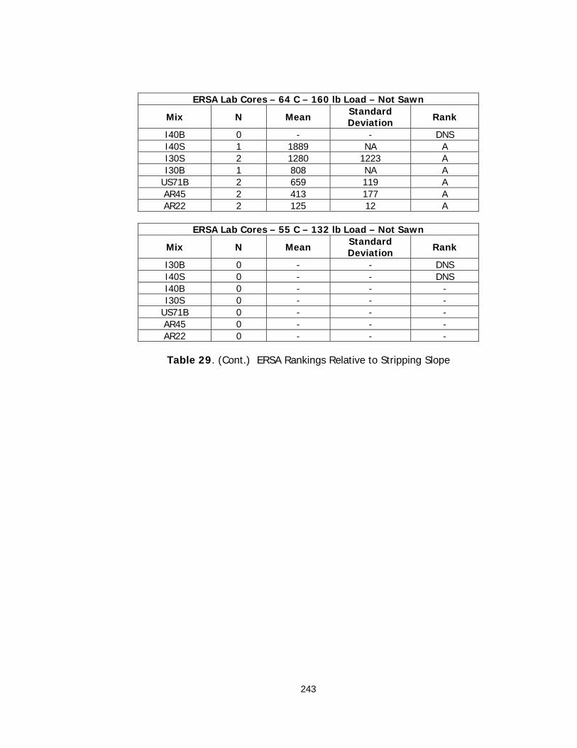
243
ERSA Lab Cores – 64 C – 160 lb Load – Not Sawn
Mix N Mean Standard Deviation Rank
I40B 0 - - DNS I40S 1 1889 NA A I30S 2 1280 1223 A I30B 1 808 NA A
US71B 2 659 119 A AR45 2 413 177 A AR22 2 125 12 A
ERSA Lab Cores – 55 C – 132 lb Load – Not Sawn
Mix N Mean Standard Deviation Rank
I30B 0 - - DNS I40S 0 - - DNS I40B 0 - - - I30S 0 - - -
US71B 0 - - - AR45 0 - - - AR22 0 - - -
Table 29. (Cont.) ERSA Rankings Relative to Stripping Slope

244
ERSA Lab Cores – 50 C – 132 lb Load – Not Sawn
Mix N Mean Standard Deviation Rank
I30B 0 - - DNS I30S 0 - - DNS I40B 0 - - DNS I40S 0 - - DNS AR45 0 - - DNS US71B 0 - - DNS AR22 8 10650 2546 A
ERSA Lab Cores – 50 C – 132 lb Load – Sawn
Mix N Mean Standard Deviation Rank
I30B 0 - - DNS I30S 0 - - DNS I40B 0 - - DNS I40S 0 - - DNS AR45 0 - - DNS US71B 1 18800 NA A AR22 4 8300 141 B
ERSA Lab Cores – 50 C – 160 lb Load – Not Sawn
Mix N Mean Standard Deviation Rank
I30B 0 - - DNS I30S 0 - - DNS I40B 0 - - DNS I40S 0 - - DNS AR45 0 - - DNS US71B 0 - - DNS AR22 2 6200 5798 A
ERSA Lab Cores – 64 C – 132 lb Load – Not Sawn
Mix N Mean Standard Deviation Rank
I30B 0 - - DNS I40B 0 - - DNS I30S 1 13300 NA A I40S 2 10800 2546 A AR45 2 9700 5515 A US71B 1 8000 NA A AR22 2 1600 1556 A
Table 30. ERSA Rankings Relative to Stripping Inflection Point

245
ERSA Lab Cores – 64 C – 160 lb Load – Not Sawn
Mix N Mean Standard Deviation Rank
I40B 0 - - DNS I30B 1 16100 NA A I40S 1 9400 NA A I30S 2 7350 5162 A
US71B 2 7300 2587 A AR45 2 6350 778 A AR22 2 650 354 A
ERSA Lab Cores – 55 C – 132 lb Load – Not Sawn
Mix N Mean Standard Deviation Rank
I30B 0 - - - I40S 0 - - - I40B 0 - - - I30S 0 - - -
US71B 0 - - - AR45 0 - - - AR22 0 - - -
Table 30. (Cont.) ERSA Rankings Relative to Stripping Inflection Point

246
ERSA Lab Cores – 50 C – 132 lb Load – Not Sawn
Mix N Mean Standard Deviation Rank
I30B 0 - - DNS I30S 0 - - DNS I40B 0 - - DNS I40S 0 - - DNS AR45 0 - - DNS US71B 0 - - DNS AR22 8 2.365 0.646 A
ERSA Lab Cores – 50 C – 132 lb Load – Sawn
Mix N Mean Standard Deviation Rank
I30B 0 - - DNS I30S 0 - - DNS I40B 0 - - DNS I40S 0 - - DNS AR45 0 - - DNS AR22 4 3.985 0.148 A US71B 1 4.640 NA A
ERSA Lab Cores – 50 C – 160 lb Load – Not Sawn
Mix N Mean Standard Deviation Rank
I30B 0 - - DNS I30S 0 - - DNS I40B 0 - - DNS I40S 0 - - DNS AR45 0 - - DNS US71B 0 - - DNS AR22 2 6.150 3.168 A
ERSA Lab Cores – 64 C – 132 lb Load – Not Sawn
Mix N Mean Standard Deviation Rank
I30B 0 - - DNS I40B 0 - - DNS I40S 2 4.830 0.396 A AR22 2 4.850 2.899 A I30S 1 5.360 NA A
US71B 1 5.500 NA A AR45 2 5.740 2.319 A
Table 31. ERSA Rankings Relative to Rut Depth at Stripping Inflection Point

247
ERSA Lab Cores – 64 C – 160 lb Load – Not Sawn
Mix N Mean Standard Deviation Rank
I40B 0 - - DNS AR22 2 2.850 1.626 A I30S 2 4.905 0.573 A I40S 1 5.330 NA A AR45 2 6.275 1.605 A I30B 1 7.380 NA A
US71B 3 7.493 2.628 A
ERSA Lab Cores – 55 C – 132 lb Load – Not Sawn
Mix N Mean Standard Deviation Rank
I30B 0 - - DNS I40S 0 - - DNS I40B 0 - - - I30S 0 - - -
US71B 0 - - - AR45 0 - - - AR22 0 - - -
Table 31. (Cont.) ERSA Rankings Relative to Rut Depth at Stripping
Inflection Point

248
Rut Depth at 20,000 Cycles – 50 C – 132 lb Load – Not Sawn
Mix N Mean Standard Deviation Rank
I30B 0 - - - I40B 0 - - - I40S 18 4.758 2.096 A
US71B 10 5.401 1.649 AB I30S 32 7.551 3.208 B AR45 21 10.947 2.291 C AR22 16 13.087 3.776 D
Rut Depth at 10,000 Cycles – 50 C – 132 lb Load – Not Sawn
Mix N Mean Standard Deviation Rank
I30B 0 - - - I40B 0 - - - I40S 18 3.268 1.252 A
US71B 10 3.441 0.921 A I30S 32 4.208 1.466 A AR45 21 5.859 2.411 B AR22 16 12.828 3.566 C
Rutting Slope – 50 C – 132 lb Load – Not Sawn
Mix N Mean Standard Deviation Rank
I30B 0 - - - I40B 0 - - - I30S 32 7809 17513 A I40S 18 7735 4897 AB
US71B 10 6246 2712 ABC AR45 21 2612 1063 BC AR22 16 717 315 C
Initial Consolidation – 50 C – 132 lb Load – Not Sawn
Mix N Mean Standard Deviation Rank
I30B 0 - - - I40B 0 - - - AR45 21 1.129 0.337 A I40S 18 1.139 0.364 A
US71B 10 1.248 0.408 A I30S 32 1.264 0.372 A AR22 16 2.296 0.653 B
Table 32. ERSA Field Sample Rankings
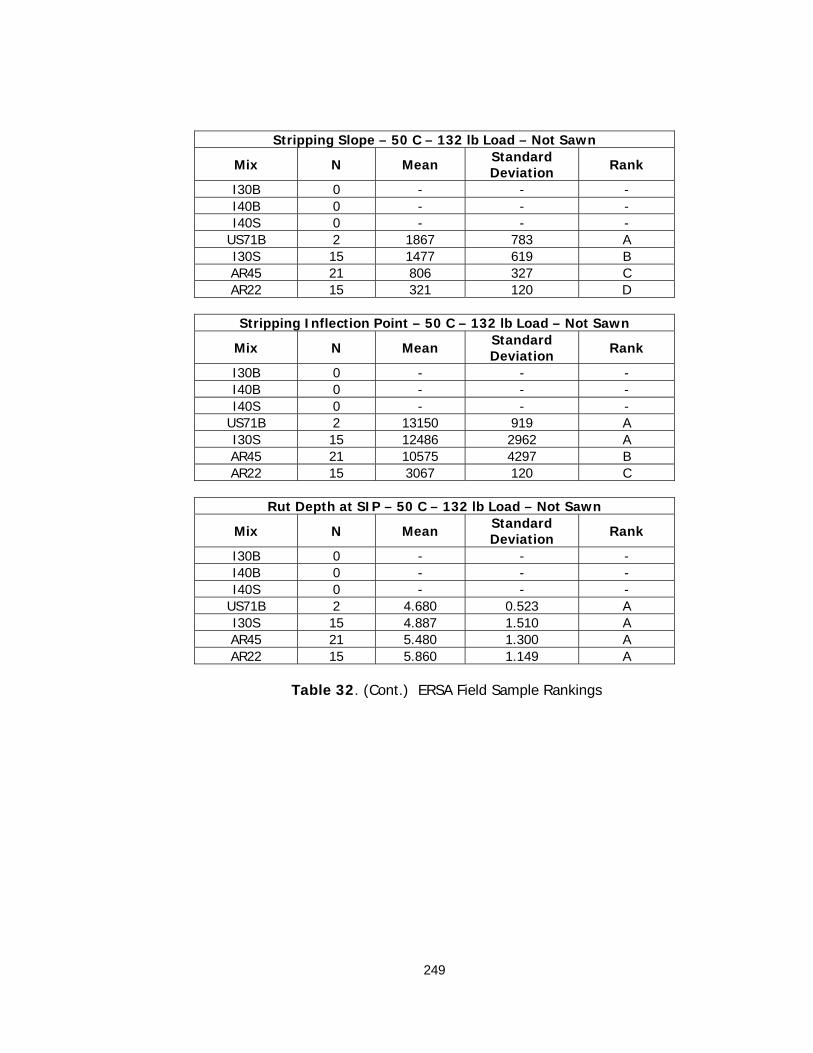
249
Stripping Slope – 50 C – 132 lb Load – Not Sawn
Mix N Mean Standard Deviation Rank
I30B 0 - - - I40B 0 - - - I40S 0 - - -
US71B 2 1867 783 A I30S 15 1477 619 B AR45 21 806 327 C AR22 15 321 120 D
Stripping Inflection Point – 50 C – 132 lb Load – Not Sawn
Mix N Mean Standard Deviation Rank
I30B 0 - - - I40B 0 - - - I40S 0 - - -
US71B 2 13150 919 A I30S 15 12486 2962 A AR45 21 10575 4297 B AR22 15 3067 120 C
Rut Depth at SIP – 50 C – 132 lb Load – Not Sawn
Mix N Mean Standard Deviation Rank
I30B 0 - - - I40B 0 - - - I40S 0 - - -
US71B 2 4.680 0.523 A I30S 15 4.887 1.510 A AR45 21 5.480 1.300 A AR22 15 5.860 1.149 A
Table 32. (Cont.) ERSA Field Sample Rankings
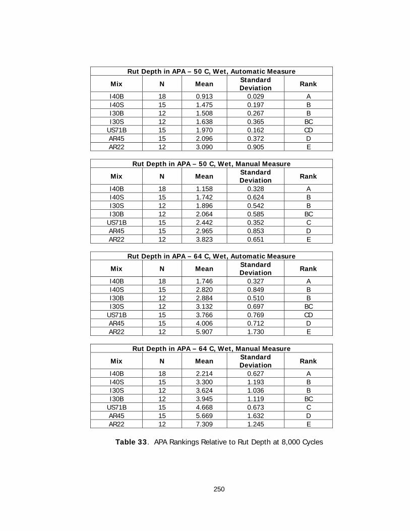
250
Rut Depth in APA – 50 C, Wet, Automatic Measure
Mix N Mean Standard Deviation Rank
I40B 18 0.913 0.029 A I40S 15 1.475 0.197 B I30B 12 1.508 0.267 B I30S 12 1.638 0.365 BC
US71B 15 1.970 0.162 CD AR45 15 2.096 0.372 D AR22 12 3.090 0.905 E
Rut Depth in APA – 50 C, Wet, Manual Measure
Mix N Mean Standard Deviation Rank
I40B 18 1.158 0.328 A I40S 15 1.742 0.624 B I30S 12 1.896 0.542 B I30B 12 2.064 0.585 BC
US71B 15 2.442 0.352 C AR45 15 2.965 0.853 D AR22 12 3.823 0.651 E
Rut Depth in APA – 64 C, Wet, Automatic Measure
Mix N Mean Standard Deviation Rank
I40B 18 1.746 0.327 A I40S 15 2.820 0.849 B I30B 12 2.884 0.510 B I30S 12 3.132 0.697 BC
US71B 15 3.766 0.769 CD AR45 15 4.006 0.712 D AR22 12 5.907 1.730 E
Rut Depth in APA – 64 C, Wet, Manual Measure
Mix N Mean Standard Deviation Rank
I40B 18 2.214 0.627 A I40S 15 3.300 1.193 B I30S 12 3.624 1.036 B I30B 12 3.945 1.119 BC
US71B 15 4.668 0.673 C AR45 15 5.669 1.632 D AR22 12 7.309 1.245 E
Table 33. APA Rankings Relative to Rut Depth at 8,000 Cycles

251
Rut Depth at 20,000 Cycles - 50 C – 100 lb Load – Not Sawn
Mix N Mean Standard Deviation Rank
AR45 5 1.692 0.306 A I40B 6 1.753 0.492 A
US71B 5 1.768 0.382 A I30B 4 1.978 0.238 A I40S 5 2.046 0.959 A I30S 4 2.430 0.559 A AR22 4 3.438 1.174 B
Rut Depth at 10,000 Cycles – 50 C – 100 lb Load – Not Sawn
Mix N Mean Standard Deviation Rank
AR45 5 1.396 0.240 A I40B 6 1.435 0.550 A
US71B 5 1.544 0.490 A I40S 5 1.632 0.869 A I30B 4 1.735 0.196 A I30S 4 1.963 0.410 AB AR22 4 2.705 0.994 B
Rutting Slope – 50 C – 100 lb Load – Not Sawn
Mix N Mean Standard Deviation Rank
AR45 5 26431 7619 A I40B 6 24601 19316 A
US71B 5 24507 11440 A AR22 4 22963 26930 A I40S 5 19129 8677 A I30B 4 13204 3043 A I30S 4 11541 3360 A
Initial Consolidation – 50 C – 100 lb Load – Not Sawn
Mix N Mean Standard Deviation Rank
AR45 5 0.550 0.144 A I40B 6 0.680 0.292 A
US71B 5 0.720 0.259 A I40S 5 0.656 0.193 A I30B 4 0.713 0.022 A I30S 4 0.823 0.213 A AR22 4 1.253 0.920 A
Table 34. ELWT Laboratory-Compacted Sample Rankings
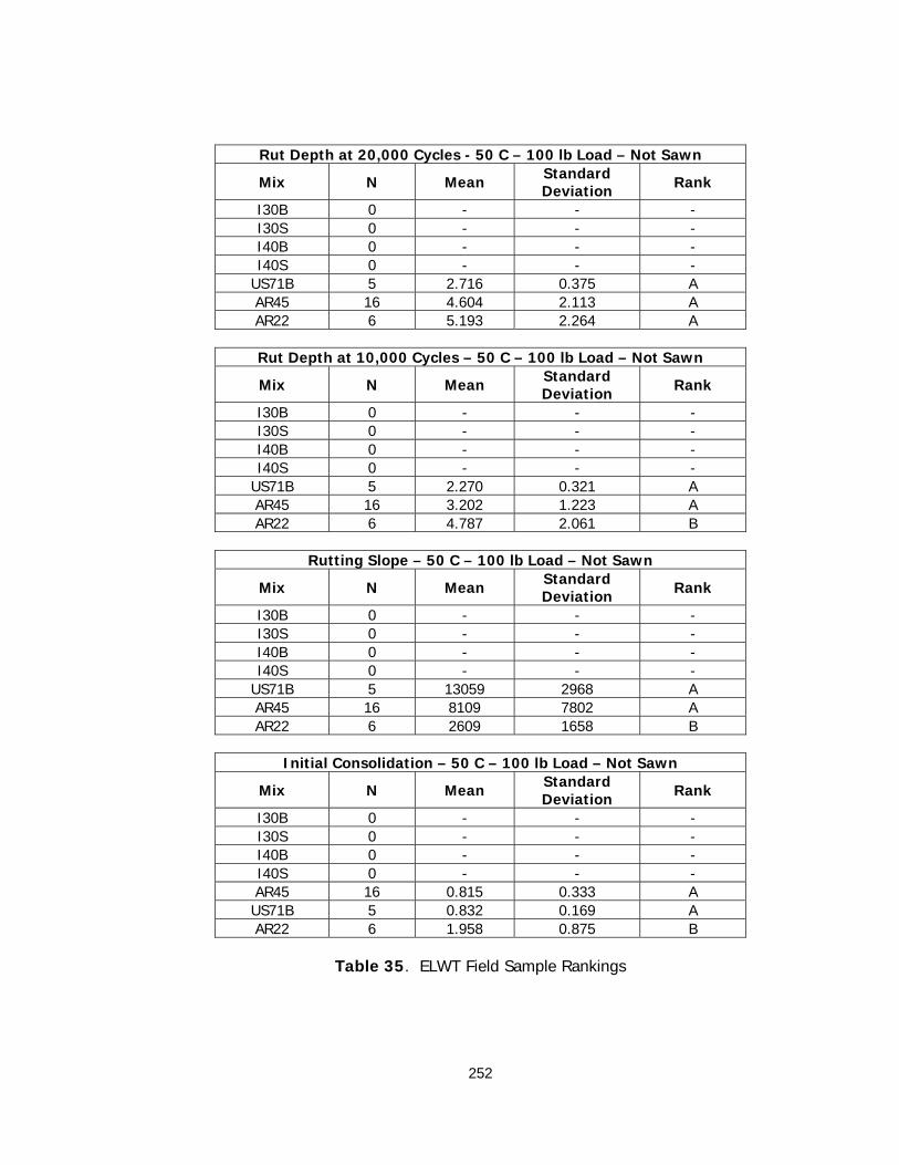
252
Rut Depth at 20,000 Cycles - 50 C – 100 lb Load – Not Sawn
Mix N Mean Standard Deviation Rank
I30B 0 - - - I30S 0 - - - I40B 0 - - - I40S 0 - - -
US71B 5 2.716 0.375 A AR45 16 4.604 2.113 A AR22 6 5.193 2.264 A
Rut Depth at 10,000 Cycles – 50 C – 100 lb Load – Not Sawn
Mix N Mean Standard Deviation Rank
I30B 0 - - - I30S 0 - - - I40B 0 - - - I40S 0 - - -
US71B 5 2.270 0.321 A AR45 16 3.202 1.223 A AR22 6 4.787 2.061 B
Rutting Slope – 50 C – 100 lb Load – Not Sawn
Mix N Mean Standard Deviation Rank
I30B 0 - - - I30S 0 - - - I40B 0 - - - I40S 0 - - -
US71B 5 13059 2968 A AR45 16 8109 7802 A AR22 6 2609 1658 B
Initial Consolidation – 50 C – 100 lb Load – Not Sawn
Mix N Mean Standard Deviation Rank
I30B 0 - - - I30S 0 - - - I40B 0 - - - I40S 0 - - - AR45 16 0.815 0.333 A US71B 5 0.832 0.169 A AR22 6 1.958 0.875 B
Table 35. ELWT Field Sample Rankings

253
AASHTO T-283 TSR (%)
Marshall Stability Ret. Stability (%)
ERSA SIP for 64C-160lb (cyc.)
Mix Mean Mix Design Mix Mean
AR45 95.4 I30S 100 I40B DNS
I40S 91.0 US71B 95.5 I30B 16100
US71B 89.0 AR22 90.4 I40S 9400
I40B 87.5 I30B 90.1 I30S 7350
AR22 85.1 AR45 81.8 US71B 7300
I30S 84.2 I40B - AR45 6350
I30B 82.7 I40S - AR22 650
Table 36. Mix Rankings by Various Moisture Sensitivity Tests

254
FIGURES

255
Figure 1. Plot of Compaction Slope as Obtained by the SGC
Per
cen
t of
Max
imu
m
Theo
reti
cal D
ensi
ty
Log Gyrations
Nmax Nini Ndes
%Gmm @ Nmax
%Gmm @ Ndes
%Gmm @ Nini
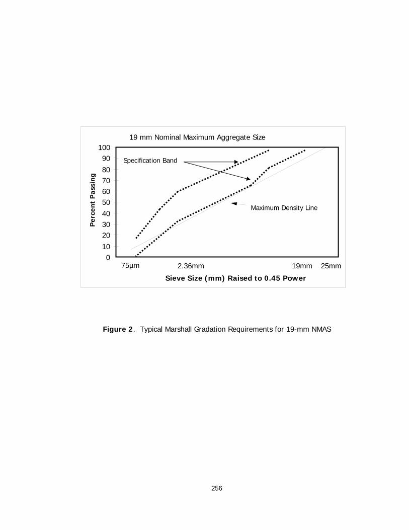
256
Figure 2. Typical Marshall Gradation Requirements for 19-mm NMAS
19 mm Nominal Maximum Aggregate Size
0
10
20 30
40
50
60
70
80
90
100
Sieve Size (mm) Raised to 0.45 Power
Per
cen
t P
assi
ng
2.36mm 19mm 25mm75µm
Maximum Density Line
Specification Band
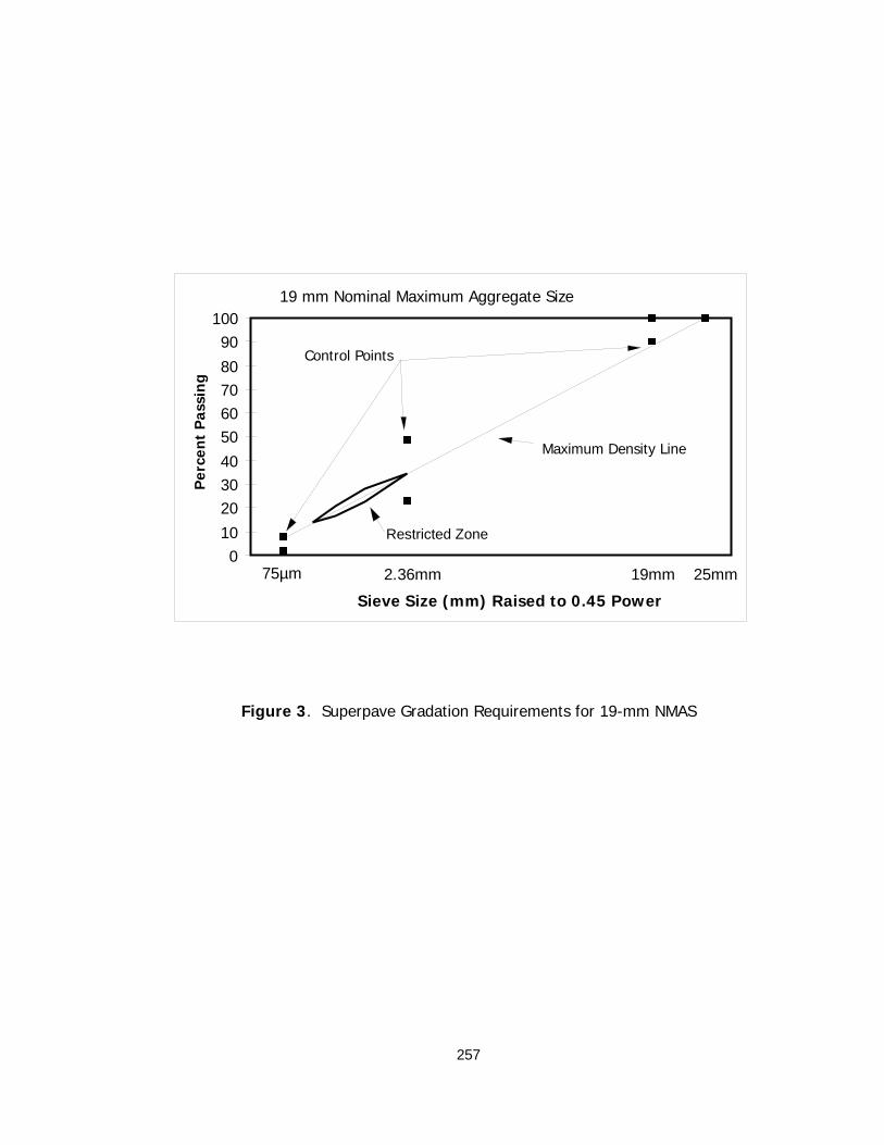
257
Figure 3. Superpave Gradation Requirements for 19-mm NMAS
19 mm Nominal Maximum Aggregate Size
0
10
20 30
40
50
60
70
80
90
100
Sieve Size (mm) Raised to 0.45 Power
Per
cen
t P
assi
ng
2.36mm 19mm 25mm75µm
Maximum Density Line
Control Points
Restricted Zone

258
Figure 4. Diagram of Indirect Tensile Stress
Induced Tensile Stress
Applied Compressive Force
Fracture Occurs Here
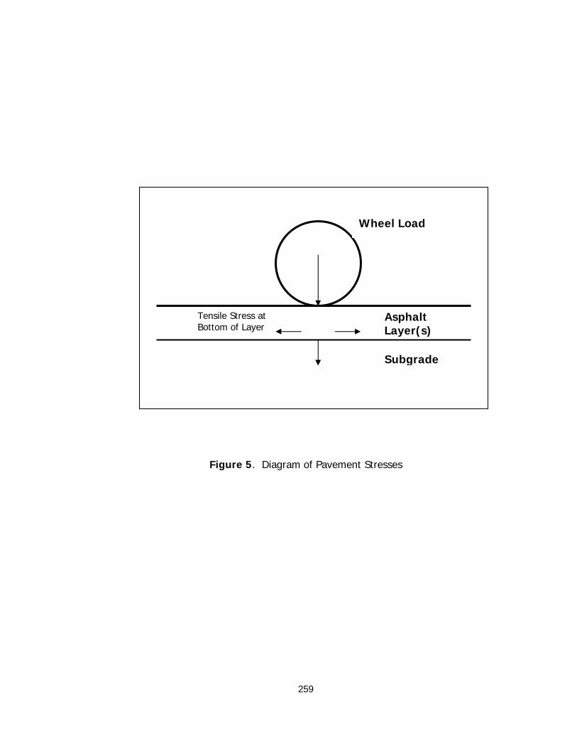
259
Figure 5. Diagram of Pavement Stresses
Subgrade
Wheel Load
Asphalt Layer(s)
Wheel Load
Tensile Stress at Bottom of Layer

260
Figure 6. Relationship of Viscous and Elastic Material Behavior
V1
V2
G*1
δ1
G*2
E1 E2
δ2
Viscous Behavior
Elastic Behavior

261
Figure 7. Rutting of the Roadway

262
Figure 8. Transverse Profile of Rutting Due to Subgrade Failure
Transverse Sample Profile
Original P ofile
Failed Profile
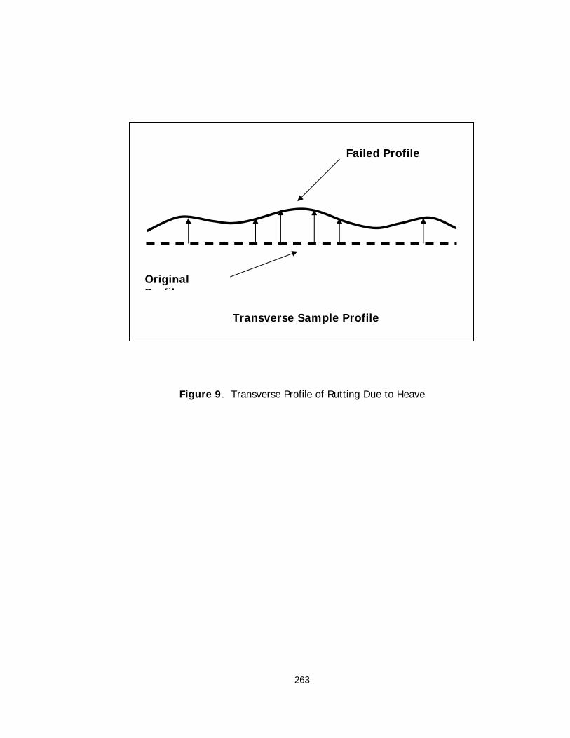
263
Figure 9. Transverse Profile of Rutting Due to Heave
Transverse Sample Profile
Original P ofile
Failed Profile
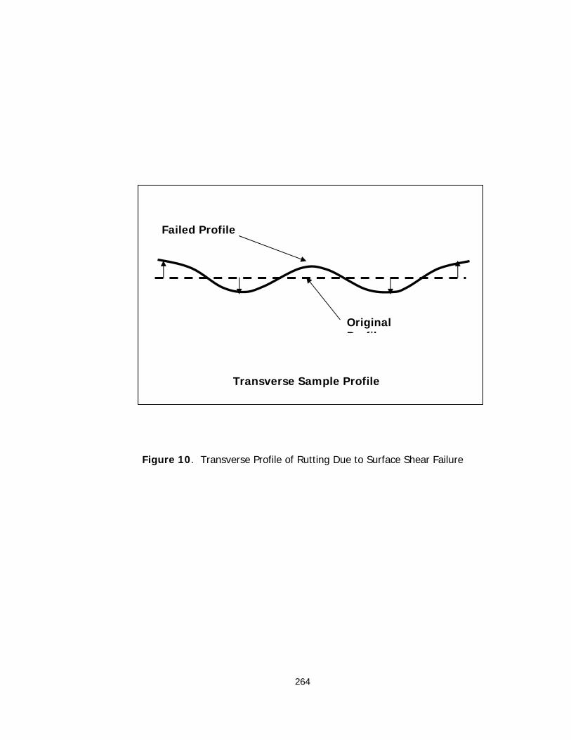
264
Figure 10. Transverse Profile of Rutting Due to Surface Shear Failure
Transverse Sample Profile
Original P ofile
Failed Profile

265
Figure 11. Transverse Profile of Rutting Due to Base Shear Failure
Transverse Sample Profile
Original P ofile
Failed Profile
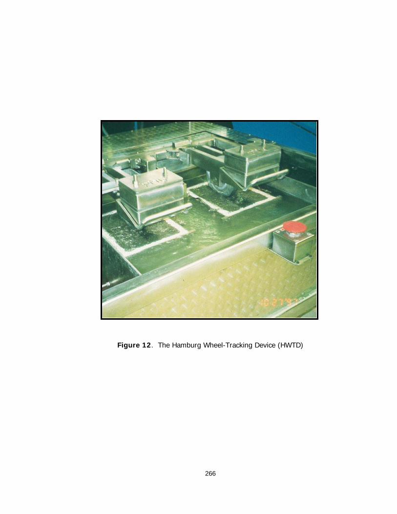
266
Figure 12. The Hamburg Wheel-Tracking Device (HWTD)

267
Figure 13. Placement of Cylindrical Specimens in Sample Tray
Core Core #2
Wheel Path

268
Figure 14. Schematic of Typical HWTD Data
Rutting Slope
Stripping Slope
Stripping Inflection Point
Initial Consolidation
Rut
Dep
th
Number of Passes
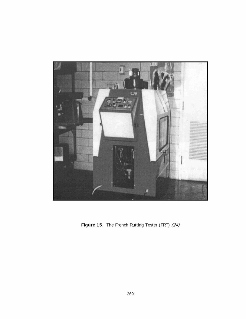
269
Figure 15. The French Rutting Tester (FRT) (24)
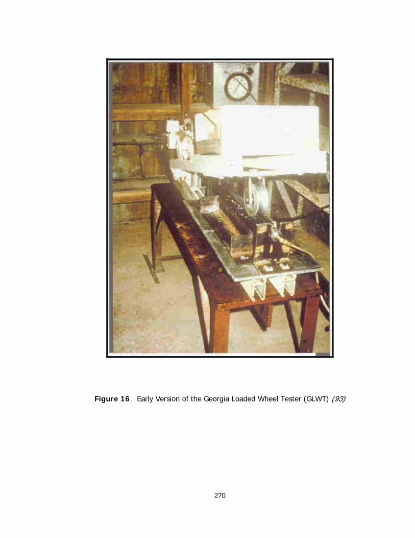
270
Figure 16. Early Version of the Georgia Loaded Wheel Tester (GLWT) (93)

271
Figure 17. Asphalt Pavement Analyzer (APA)

272
Figure 18. Schematic of Typical APA Wheel-Tracking Data
Number of Passes
Ru
t D
epth

273
Figure 19. Model Mobile Load Simulator (MMLS3) (24)

274
Figure 20. Evaluator of Rutting and Stripping in Asphalt (ERSA)

275
Figure 21. Schematic of Sample Placement With and Without Sawn Faces
No Sawn Faces Sawn Faces

276
Figure 22. Locations of Sampling Sites
ϑ
ϑϑ
ϑϑ
US71B Springdale
AR45 Hartford
AR22 Dardanelle
I-40 Morgan
I-30 Little Rock

277
Figure 23. Sample Testing Configuration
1 2 3 4 5 6
1 2 3 4
5 6 7 8
3 4
Sawn vs.
Unsawn
ERSA vs.
ELWT
1 2 3 4 5 6
T-283
APA Dry
1 2
Air Voids
X X
1 2 3 4 5 6
50 C / 160 lb 64 C / 132 lb 64 C / 160 lb
For Each Mix
For Each Mix
APA

278
Figure 24. Cutting Field Cores

279
Figure 25. Cutting and Trimming Field Slabs

280
Figure 26. Laboratory Sample Preparation

281
Figure 27. The Wire Line Principle
Wire Line Principle
Transverse Profile
Wire
Measure the maximum distance between the wire and pavement surface for
each wheel path.
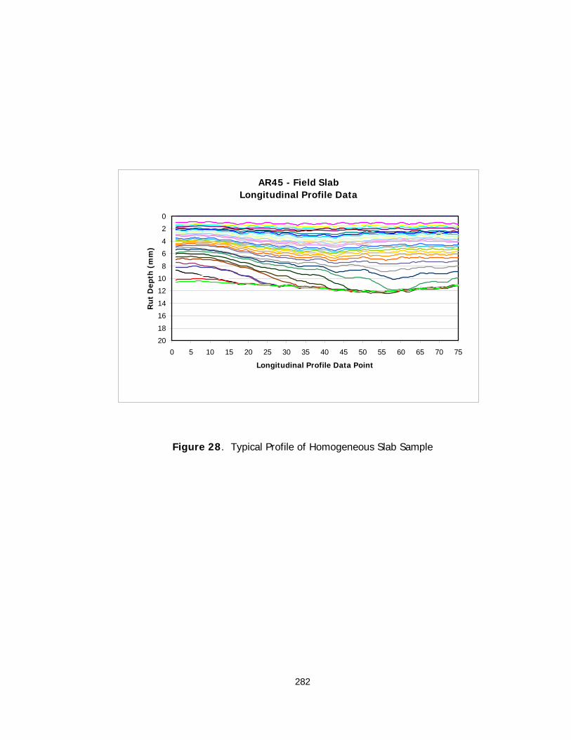
282
AR45 - Field SlabLongitudinal Profile Data
0
2
4
6
8
10
12
14
16
18
200 5 10 15 20 25 30 35 40 45 50 55 60 65 70 75
Longitudinal Profile Data Point
Ru
t D
epth
(m
m)
Figure 28. Typical Profile of Homogeneous Slab Sample

283
AR45 - Field CoresLongitudinal Profile Data
0
2
4
6
8
10
12
14
16
18
200 5 10 15 20 25 30 35 40 45 50 55 60 65 70 75
Longitudinal Profile Data Point
Rut
Dep
th (
mm
)
Figure 29. Typical Profile of Homogeneous Core Sample

284
I30 - Field SlabLongitudinal Profile Data
0
2
4
6
8
10
12
14
16
18
200 5 10 15 20 25 30 35 40 45 50 55 60 65 70 75
Longitudinal Profile Data Point
Ru
t D
epth
(m
m)
Figure 30. Typical Profile of Non-Homogeneous Slab Sample

285
US71B - Field CoresLongitudinal Profile Data
0
2
4
6
8
10
12
14
16
18
200 5 10 15 20 25 30 35 40 45 50 55 60 65 70 75
Longitudinal Profile Data Point
Rut
Dep
th (
mm
)
Figure 31. Typical Profile of Non-Homogeneous Core Sample

286
AR22 - SGC CoresLongitudinal Profile Data
0
2
4
6
8
10
12
14
16
18
200 5 10 15 20 25 30 35 40 45 50 55 60 65 70 75
Longitudinal Profile Data Point
Ru
t D
epth
(m
m)
Figure 32. Profile of Cylindrical Specimens with Stable Interface

287
AR45 - SGC CoresLongitudinal Profile Data
0
2
4
6
8
10
12
14
16
18
200 5 10 15 20 25 30 35 40 45 50 55 60 65 70 75
Longitudinal Profile Data Point
Rut
Dep
th (
mm
)
Figure 33. Profile of Cylindrical Specimens with Unstable Interface

288
AR22 - Sawn SGC SampleLongitudinal Profile Data
0
2
4
6
8
10
12
14
16
18
200 5 10 15 20 25 30 35 40 45 50 55 60 65 70 75
Longitudinal Profile Data Point
Rut
Dep
th (
mm
)
Figure 34. Profile of Sawn Cylindrical Specimens
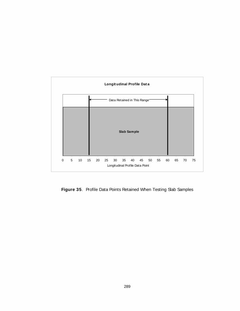
289
Longitudinal Profile Data
0 5 10 15 20 25 30 35 40 45 50 55 60 65 70 75
Longitudinal Profile Data Point
Data Retained in This Range
Slab Sample
Figure 35. Profile Data Points Retained When Testing Slab Samples
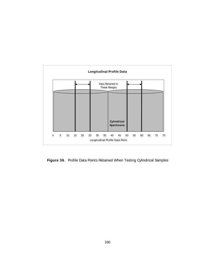
290
Longitudinal Profile Data
0 5 10 15 20 25 30 35 40 45 50 55 60 65 70 75
Longitudinal Profile Data Point
Data Retained in These Ranges
Cylindrical Specimens
Figure 36. Profile Data Points Retained When Testing Cylindrical Samples

291
Longitudinal Profile Data
0 5 10 15 20 25 30 35 40 45 50 55 60 65 70 75
Longitudinal Profile Data Point
Data Retained in These Ranges
SawnCylindrical Specimens
Figure 37. Profile Data Points Retained When Testing Sawn Cylindrical Samples

292
AR22 - Dardanelle - Sample B3 - 2ERSA - 50 C and 132 lb Load - Field Slab
0
2
4
6
8
10
12
14
16
18
200 2000 4000 6000 8000 10000 12000 14000 16000 18000 20000 22000
Number of Cycles
Rut D
epth
(mm
)
Rutting Slope
Stripping Slope
SIP
Figure 38. Sample ERSA Data

293
AR22 - Dardanelle - ERSA Lab CoresNot Sawn, 50 C and 132 lb Load
y = 1.6504x - 5.0937R2 = 0.0893
0
2
4
6
8
10
12
2 3 4 5 6 7 8 9 10 11 12
Air Voids (%)
Rut
Dep
th a
t 20
,000
Cyc
les
(mm
)
Figure 39. Rut Depth at 20,000 Cycles vs. Air Voids for AR22

294
AR45 - Hartford - ERSA Lab CoresNot Sawn, 50 C and 132 lb Load
y = 0.2525x + 0.3441R2 = 0.5525
0
2
4
6
8
10
12
2 3 4 5 6 7 8 9 10 11 12
Air Voids (%)
Rut
Dep
th a
t 20
,000
Cyc
les
(mm
)
Figure 40. Rut Depth at 20,000 Cycles vs. Air Voids for AR45

295
I-30 Binder - ERSA Lab CoresNot Sawn, 50 C and 132 lb Load
y = 0.5836x - 1.2822R2 = 0.2627
0
2
4
6
8
10
12
2 3 4 5 6 7 8 9 10 11 12
Air Voids (%)
Rut
Dep
th a
t 20
,000
Cyc
les
(mm
)
Figure 41. Rut Depth at 20,000 Cycles vs. Air Voids for I30B

296
I-30 Surface - ERSA Lab Cores Not Sawn, 50 C and 132 lb Load
y = -0.0053x + 2.8458R2 = 5E-05
0
2
4
6
8
10
12
2 3 4 5 6 7 8 9 10 11 12
Air Voids (%)
Rut
Dep
th a
t 20
,000
Cyc
les
(mm
)
Figure 42. Rut Depth at 20,000 Cycles vs. Air Voids for I30S

297
I-40 Binder - ERSA Lab CoresNot Sawn, 50 C and 132 lb Load
y = 0.2698x - 0.3927R2 = 0.2803
0
2
4
6
8
10
12
2 3 4 5 6 7 8 9 10 11 12
Air Voids (%)
Rut
Dep
th a
t 20
,000
Cyc
les
(mm
)
Figure 43. Rut Depth at 20,000 Cycles vs. Air Voids for I40B

298
I-40 Surface - ERSA Lab CoresNot Sawn, 50 C and 132 lb Load
y = 0.124x + 1.629R2 = 0.0138
0
2
4
6
8
10
12
2 3 4 5 6 7 8 9 10 11 12
Air Voids (%)
Rut
Dep
th a
t 20
,000
Cyc
les
(mm
)
Figure 44. Rut Depth at 20,000 Cycles vs. Air Voids for I40S

299
US71B - Springdale - ERSA Lab CoresNot Sawn, 50 C and 132 lb Load
y = 0.0543x + 2.5869R2 = 0.0309
0
2
4
6
8
10
12
2 3 4 5 6 7 8 9 10 11 12
Air Voids (%)
Rut
Dep
th a
t 20
,000
Cyc
les
Figure 45. Rut Depth at 20,000 Cycles vs. Air Voids for US71B

300
AR22 - Dardanelle - ERSA Lab CoresNot Sawn, 50 C and 132 lb Load
y = 1.5565x - 7.5202R2 = 0.1236
0
2
4
6
8
10
12
2 3 4 5 6 7 8 9 10 11 12
Air Voids (%)
Rut
Dep
th a
t 10
,000
Cyc
les
(mm
)
Figure 46. Rut Depth at 10,000 Cycles vs. Air Voids for AR22

301
AR45 - Hartford - ERSA Lab CoresNot Sawn, 50 C and 132 lb Load
y = 0.2453x - 0.137R2 = 0.6314
0
2
4
6
8
10
12
2 3 4 5 6 7 8 9 10 11 12
Air Voids (%)
Rut
Dep
th a
t 10
,000
Cyc
les
(mm
)
Figure 47. Rut Depth at 10,000 Cycles vs. Air Voids for AR45
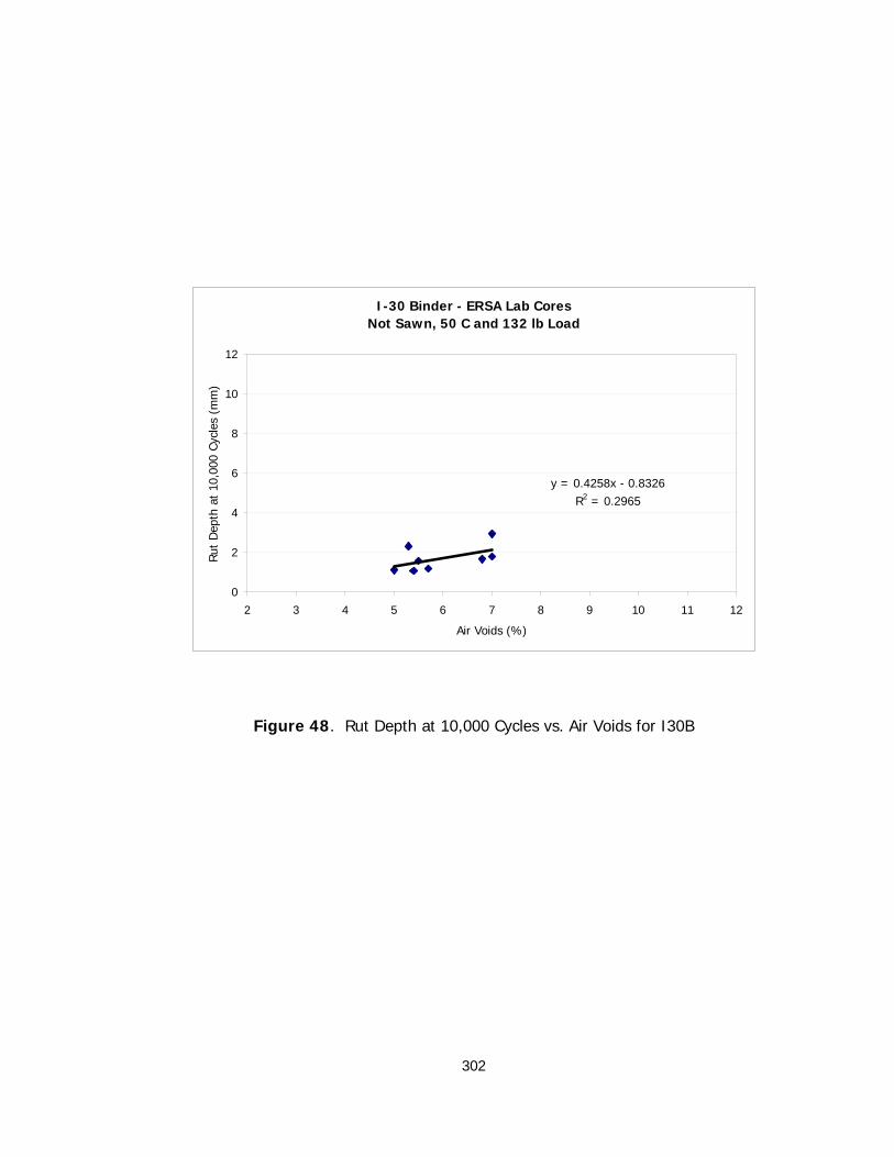
302
I-30 Binder - ERSA Lab CoresNot Sawn, 50 C and 132 lb Load
y = 0.4258x - 0.8326R2 = 0.2965
0
2
4
6
8
10
12
2 3 4 5 6 7 8 9 10 11 12
Air Voids (%)
Rut
Dep
th a
t 10
,000
Cyc
les
(mm
)
Figure 48. Rut Depth at 10,000 Cycles vs. Air Voids for I30B
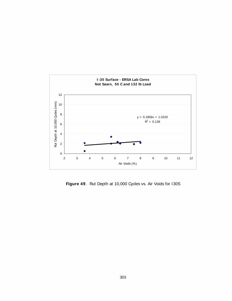
303
I-30 Surface - ERSA Lab Cores Not Sawn, 50 C and 132 lb Load
y = 0.1856x + 1.0102R2 = 0.139
0
2
4
6
8
10
12
2 3 4 5 6 7 8 9 10 11 12
Air Voids (%)
Rut
Dep
th a
t 10
,000
Cyc
les
(mm
)
Figure 49. Rut Depth at 10,000 Cycles vs. Air Voids for I30S

304
I-40 Binder - ERSA Lab CoresNot Sawn, 50 C and 132 lb Load
y = 0.2203x - 0.397R2 = 0.3556
0
2
4
6
8
10
12
2 3 4 5 6 7 8 9 10 11 12
Air Voids (%)
Rut
Dep
th a
t 10
,000
Cyc
les
(mm
)
Figure 50. Rut Depth at 10,000 Cycles vs. Air Voids for I40B
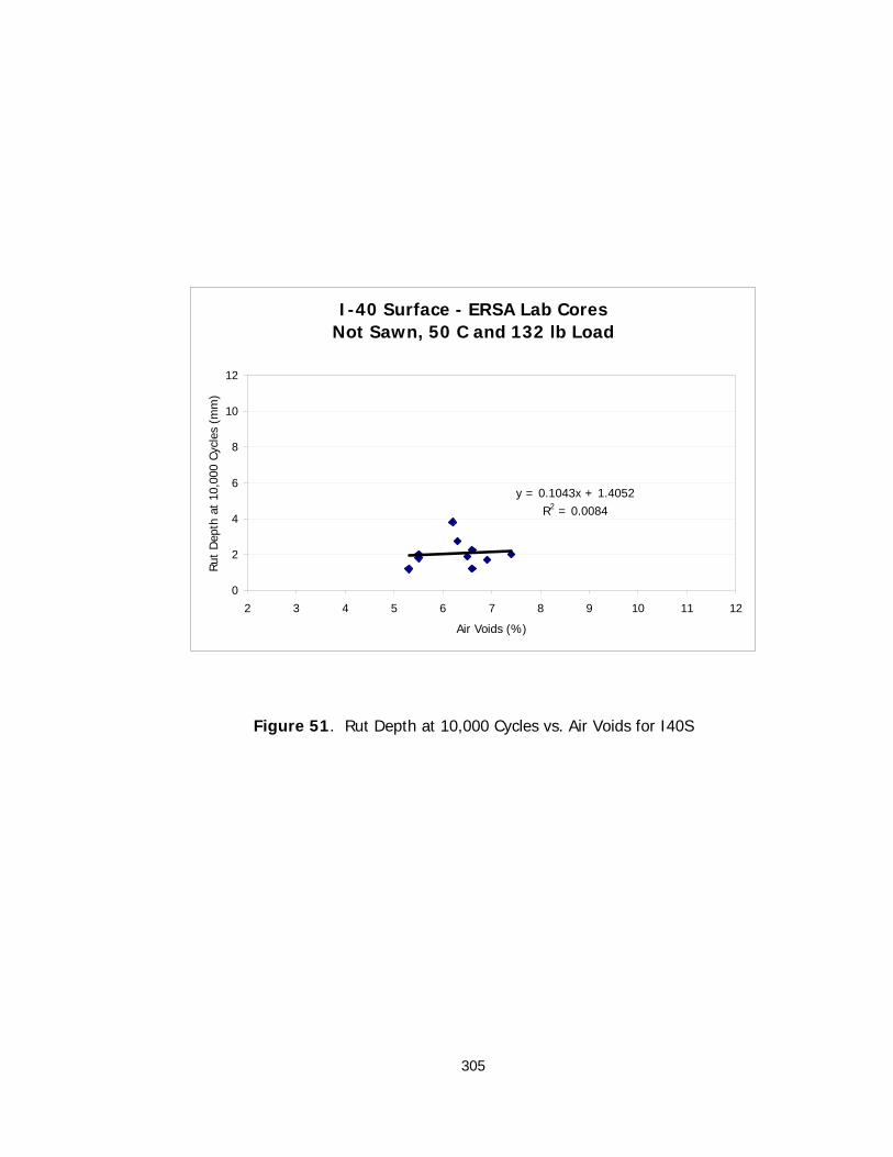
305
I-40 Surface - ERSA Lab CoresNot Sawn, 50 C and 132 lb Load
y = 0.1043x + 1.4052R2 = 0.0084
0
2
4
6
8
10
12
2 3 4 5 6 7 8 9 10 11 12
Air Voids (%)
Rut
Dep
th a
t 10
,000
Cyc
les
(mm
)
Figure 51. Rut Depth at 10,000 Cycles vs. Air Voids for I40S

306
US71B - Springdale - ERSA Lab CoresNot Sawn, 50 C and 132 lb Load
y = 0.0971x + 1.6102R2 = 0.1644
0
2
4
6
8
10
12
2 3 4 5 6 7 8 9 10 11 12
Air Voids (%)
Rut
Dep
th a
t 10
,000
Cyc
les
Figure 52. Rut Depth at 10,000 Cycles vs. Air Voids for US71B

307
AR22 - Dardanelle - ERSA Lab CoresNot Sawn, 50 C and 132 lb Load
y = -4543.8x + 39058R2 = 0.2028
0
5000
10000
15000
20000
25000
30000
2 3 4 5 6 7 8 9 10 11 12
Air Voids (%)
Rut
ting
Slop
e (c
yc/m
m)
Figure 53. Rutting Slope vs. Air Voids for AR22

308
AR45 - Hartford - ERSA Lab CoresNot Sawn, 50 C and 132 lb Load
y = -66.91x + 15523R2 = 0.0004
0
5000
10000
15000
20000
25000
30000
2 3 4 5 6 7 8 9 10 11 12
Air Voids (%)
Rut
ting
Slop
e (c
yc/m
m)
Figure 54. Rutting Slope vs. Air Voids for AR45

309
I-30 Binder - ERSA Lab CoresNot Sawn, 50 C and 132 lb Load
y = -7103.7x + 57486R2 = 0.5096
0
5000
10000
15000
20000
25000
30000
2 3 4 5 6 7 8 9 10 11 12
Air Voids (%)
Rutt
ing
Slop
e (c
yc/m
m)
Figure 55. Rutting Slope vs. Air Voids for I30B

310
I-30 Surface - ERSA Lab Cores Not Sawn, 50 C and 132 lb Load
y = -1395.3x + 32559R2 = 0.0052
0
5000
10000
15000
20000
25000
30000
2 3 4 5 6 7 8 9 10 11 12
Air Voids (%)
Rut
ting
Slop
e (c
yc/m
m)
Figure 56. Rutting Slope vs. Air Voids for I30S

311
I-40 Binder - ERSA Lab CoresNot Sawn, 50 C and 132 lb Load
y = -1907.5x + 34561R2 = 0.0656
0
5000
10000
15000
20000
25000
30000
2 3 4 5 6 7 8 9 10 11 12
Air Voids (%)
Rut
ting
Slop
e (c
yc/m
m)
Figure 57. Rutting Slope vs. Air Voids for I40B
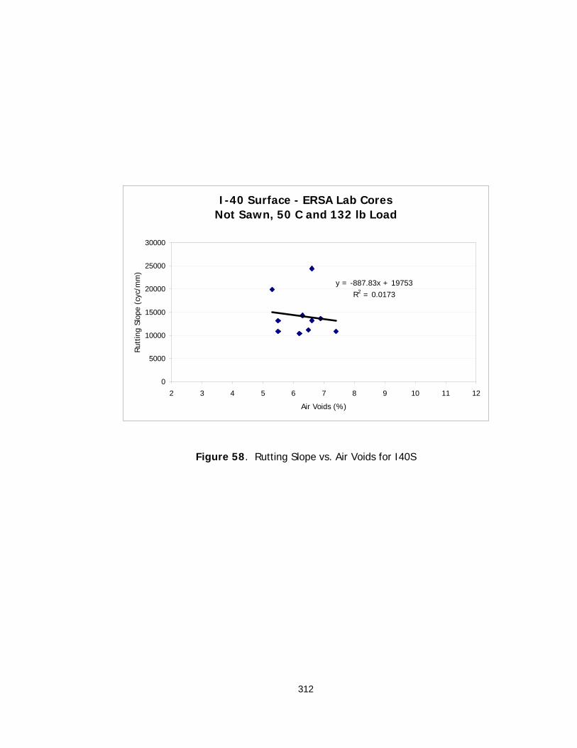
312
I-40 Surface - ERSA Lab CoresNot Sawn, 50 C and 132 lb Load
y = -887.83x + 19753R2 = 0.0173
0
5000
10000
15000
20000
25000
30000
2 3 4 5 6 7 8 9 10 11 12
Air Voids (%)
Rutt
ing
Slop
e (c
yc/m
m)
Figure 58. Rutting Slope vs. Air Voids for I40S
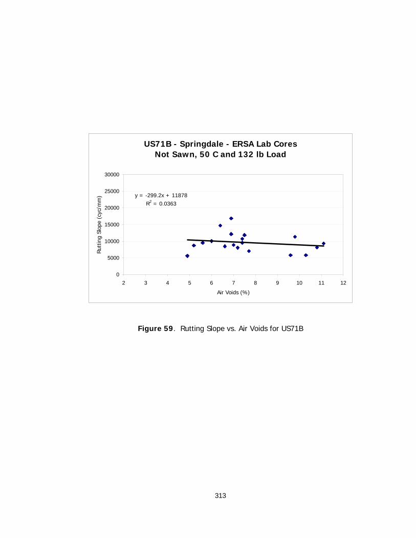
313
US71B - Springdale - ERSA Lab CoresNot Sawn, 50 C and 132 lb Load
y = -299.2x + 11878R2 = 0.0363
0
5000
10000
15000
20000
25000
30000
2 3 4 5 6 7 8 9 10 11 12
Air Voids (%)
Rutt
ing
Slop
e (c
yc/m
m)
Figure 59. Rutting Slope vs. Air Voids for US71B

314
AR22 - Dardanelle - ERSA Lab CoresNot Sawn, 50 C and 132 lb Load
y = 0.072x + 0.5365R2 = 0.0024
0
1
2
3
4
5
6
2 3 4 5 6 7 8 9 10 11 12
Air Voids (%)
Initi
al C
onso
lidat
ion
(mm
)
Figure 60. Initial Consolidation vs. Air Voids for AR22

315
AR45 - Hartford - ERSA Lab CoresNot Sawn, 50 C and 132 lb Load
y = 0.1376x - 0.2696R2 = 0.4117
0
1
2
3
4
5
6
2 3 4 5 6 7 8 9 10 11 12
Air Voids (%)
Initi
al C
onso
lidat
ion
(mm
)
Figure 61. Initial Consolidation vs. Air Voids for AR45

316
I-30 Binder - ERSA Lab CoresNot Sawn, 50 C and 132 lb Load
y = 0.1922x - 0.355R2 = 0.1388
0
1
2
3
4
5
6
2 3 4 5 6 7 8 9 10 11 12
Air Voids (%)
Initi
al C
onso
lidat
ion
(mm
)
Figure 62. Initial Consolidation vs. Air Voids for I30B
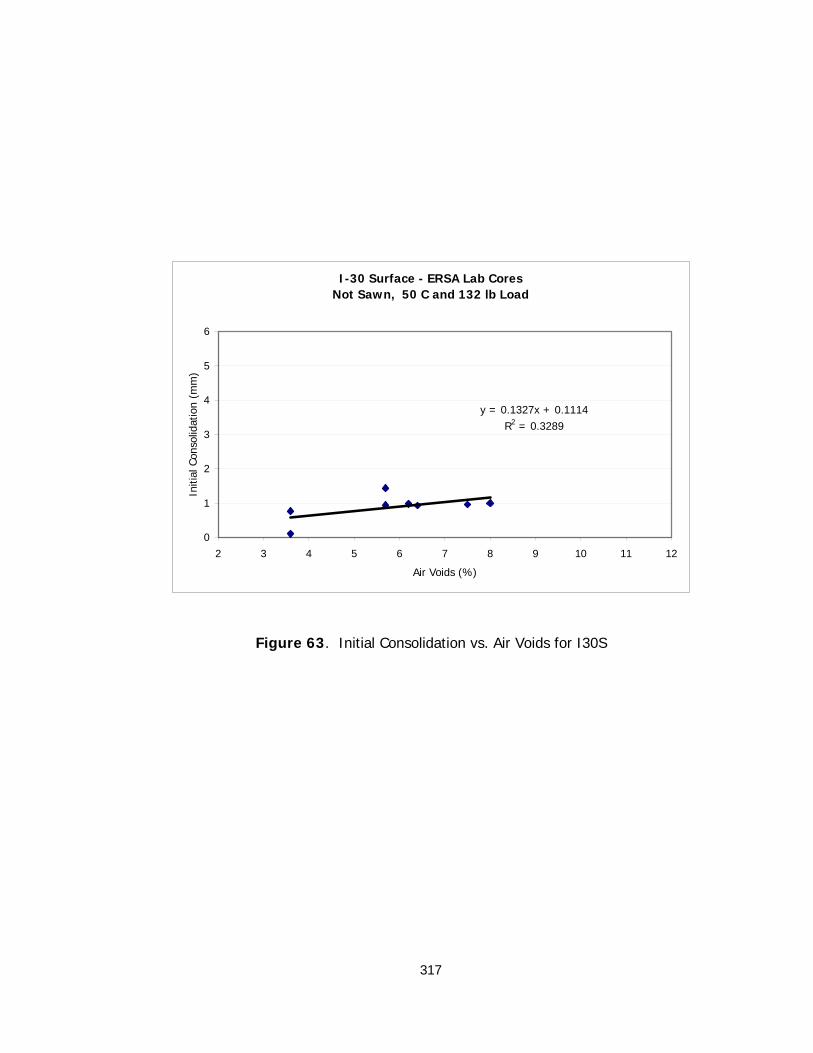
317
I-30 Surface - ERSA Lab Cores Not Sawn, 50 C and 132 lb Load
y = 0.1327x + 0.1114R2 = 0.3289
0
1
2
3
4
5
6
2 3 4 5 6 7 8 9 10 11 12
Air Voids (%)
Initi
al C
onso
lidat
ion
(mm
)
Figure 63. Initial Consolidation vs. Air Voids for I30S

318
I-40 Binder - ERSA Lab CoresNot Sawn, 50 C and 132 lb Load
y = -0.0035x + 0.5046R2 = 0.0005
0
1
2
3
4
5
6
2 3 4 5 6 7 8 9 10 11 12
Air Voids (%)
Initi
al C
onso
lidat
ion
(mm
)
Figure 64. Initial Consolidation vs. Air Voids for I40B

319
I-40 Surface - ERSA Lab CoresNot Sawn, 50 C and 132 lb Load
y = 0.1095x + 0.0735R2 = 0.073
0
1
2
3
4
5
6
2 3 4 5 6 7 8 9 10 11 12
Air Voids (%)
Initi
al C
onso
lidat
ion
(mm
)
Figure 65. Initial Consolidation vs. Air Voids for I40S

320
US71B - Springdale - ERSA Lab CoresNot Sawn, 50 C and 132 lb Load
y = 0.05x + 0.5885R2 = 0.1429
0
1
2
3
4
5
6
2 3 4 5 6 7 8 9 10 11 12
Air Voids (%)
Initi
al C
onso
lidat
ion
(mm
)
Figure 66. Initial Consolidation vs. Air Voids for US71B
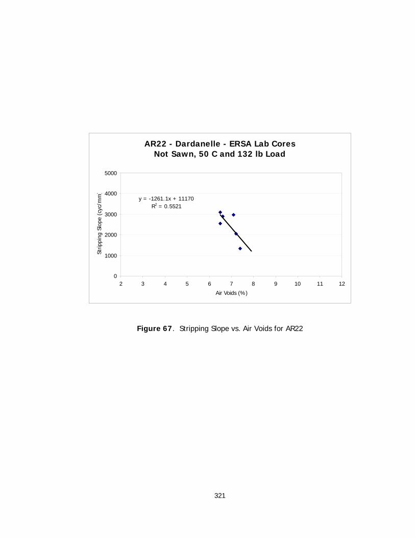
321
AR22 - Dardanelle - ERSA Lab CoresNot Sawn, 50 C and 132 lb Load
y = -1261.1x + 11170R2 = 0.5521
0
1000
2000
3000
4000
5000
2 3 4 5 6 7 8 9 10 11 12
Air Voids (%)
Strip
ping
Slo
pe (
cyc/
mm
)
Figure 67. Stripping Slope vs. Air Voids for AR22

322
AR22 - Dardanelle - ERSA Lab CoresNot Sawn, 50 C and 132 lb Load
y = -3849.9x + 37150R2 = 0.3605
0
5000
10000
15000
20000
2 3 4 5 6 7 8 9 10 11 12
Air Voids (%)
Strip
ping
Inf
lect
ion
Poin
t (c
yc)
Figure 68. Stripping Inflection Point vs. Air Voids for AR22

323
AR22 - Dardanelle - ERSA Lab CoresNot Sawn, 50 C and 132 lb Load
y = 0.072x + 0.5365R2 = 0.0024
0
1
2
3
4
5
6
7
8
2 3 4 5 6 7 8 9 10 11 12
Air Voids (%)
Rut
Dep
th a
t SI
P (m
m)
Figure 69. Rut Depth at Stripping Inflection Point vs. Air Voids for AR22

324
0
2
4
6
8
10
12
14
16
18
20
Rut
Dep
th a
t 20
,000
Cyc
les
(mm
)
AR22 AR45 I30B I30S I40B I40S US71B
Mix Identification
Effect of Temperature and Load on Rut Depth at 20,000 Cycles
T=50 CL=132 lb
T=50 CL=160 lb
T=64 CL=132 lb
T=64 CL=160 lb
Figure 70. Effect of Temperature and Load on Rut Depth at 20,000 Cycles

325
0
2
4
6
8
10
12
14
16
18
20
Rut
Dep
th a
t 10
,000
Cyc
les
(mm
)
AR22 AR45 I30B I30S I40B I40S US71BMix Identification
Effect of Temperature and Load on Rut Depth at 10,000 Cycles
T=50 CL=132 lbT=50 CL=160 lbT=64 CL=132 lbT=64 CL=160 lb
Figure 71. Effect of Temperature and Load on Rut Depth at 10,000 Cycles

326
0
5000
10000
15000
20000
25000
30000
Rut
ting
Slop
e (c
yc/m
m)
AR22 AR45 I30B I30S I40B I40S US71BMix Identification
Effect of Temperature and Load on Rutting Slope
T=50 CL=132 lbT=50 CL=160 lbT=64 CL=132 lbT=64 CL=160 lb
Figure 72. Effect of Temperature and Load on Rutting Slope
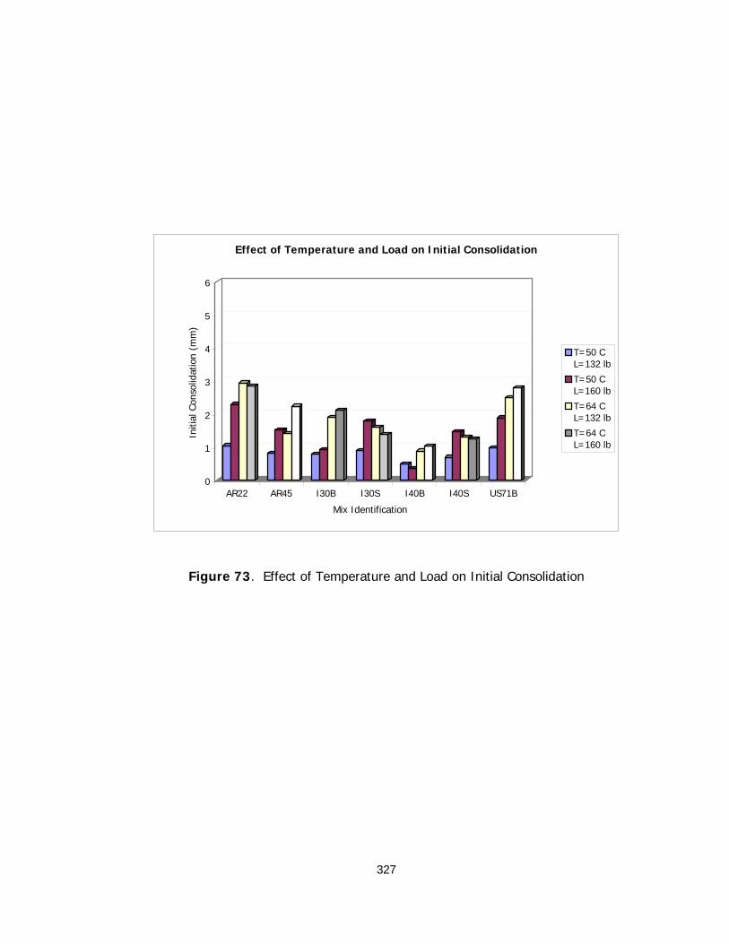
327
0
1
2
3
4
5
6
Initi
al C
onso
lidat
ion
(mm
)
AR22 AR45 I30B I30S I40B I40S US71B
Mix Identification
Effect of Temperature and Load on Initial Consolidation
T=50 CL=132 lb
T=50 CL=160 lb
T=64 CL=132 lb
T=64 CL=160 lb
Figure 73. Effect of Temperature and Load on Initial Consolidation

328
0
1000
2000
3000
4000
5000
Strip
ping
Slo
pe (
cyc/
mm
)
AR22 AR45 I30B I30S I40B I40S US71B
Mix Identification
Effect of Temperature and Load on Stripping Slope
T=50 CL=132 lb
T=50 CL=160 lb
T=64 CL=132 lb
T=64 CL=160 lb
Figure 74. Effect of Temperature and Load on Stripping Slope

329
0
5000
10000
15000
20000
Strip
ping
Inf
lect
ion
Poin
t (c
yc)
AR22 AR45 I30B I30S I40B I40S US71BMix Identification
Effect of Temperature and Load on Stripping Inflection Point
T=50 CL=132 lbT=50 CL=160 lbT=64 CL=132 lbT=64 CL=160 lb
Figure 75. Effect of Temperature and Load on Stripping Inflection Point

330
0
1
2
3
4
5
6
7
8
Rut
Dep
th a
t SI
P (m
m)
AR22 AR45 I30B I30S I40B I40S US71BMix Identification
Effect of Temperature and Load on Rut Depth at SIP
T=50 CL=132 lbT=50 CL=160 lbT=64 CL=132 lbT=64 CL=160 lb
Figure 76. Effect of Temperature and Load on Rut Depth at Stripping Inflection Point

331
0
1
2
3
4
5
6
7
8
9
10
Fina
l Rut
Dep
th (
mm
)
AR22 AR45 I30B I30S I40B I40S US71B
Mix Identification
Comparison of Wheel TypeLab-Compacted Cylindrical Specimens
APA - 50 CAuto Meas.
ELWT - 50 C
ERSA - 50 C
Figure 77. Comparison of Wheel Type - Testing Laboratory-Compacted Cylindrical Specimens (APA Tests at 50 C Based on
Automatic Measurements)
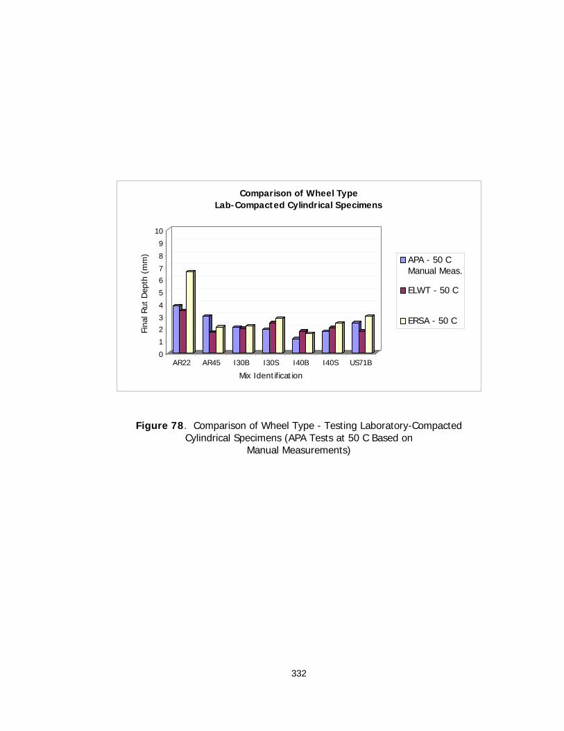
332
0
1
23
4
5
67
8
9
10
Fina
l Rut
Dep
th (
mm
)
AR22 AR45 I30B I30S I40B I40S US71B
Mix Identification
Comparison of Wheel TypeLab-Compacted Cylindrical Specimens
APA - 50 CManual Meas.
ELWT - 50 C
ERSA - 50 C
Figure 78. Comparison of Wheel Type - Testing Laboratory-Compacted Cylindrical Specimens (APA Tests at 50 C Based on
Manual Measurements)

333
0
1
2
3
4
5
6
7
8
9
10
Fina
l Rut
Dep
th (
mm
)
AR22 AR45 I30B I30S I40B I40S US71B
Mix Identification
Comparison of Wheel TypeLab-Compacted Cylindrical Specimens
APA - 64 CAuto Meas.
ELWT - 50 C
ERSA - 50 C
Figure 79. Comparison of Wheel Type - Testing Laboratory-Compacted Cylindrical Specimens (APA Tests at 64 C by TEM Based on
Automatic Measurements)

334
0
12
3
4
56
7
8
910
Fina
l Rut
Dep
th (
mm
)
AR22 AR45 I30B I30S I40B I40S US71B
Mix Identification
Comparison of Wheel TypeLab-Compacted Cylindrical Specimens
APA - 64 CManual Meas.
ELWT - 50 C
ERSA - 50 C
Figure 80. Comparison of Wheel Type - Testing Laboratory-Compacted Cylindrical Specimens (APA Tests at 64 C by TEM Based on
Manual Measurements)

335
Rut Depth vs. VMA (%)ERSA Lab Cores Tested at 50 C and 132 lb Load
0
2
4
6
8
10
12
14
16
18
20
12 14 16 18 20 22 24
VMA (%)
Rut
Dep
th (
mm
)
Figure 81. Relationship of VMA and Rut Depth at 20,000 Cycles in ERSA Testing Laboratory-Compacted Cores at 50 C and a 132 lb Load

336
Rut Depth vs. Binder Content (%)ERSA Lab Cores Tested at 50 C and 132 lb Load
0
2
4
6
8
10
12
14
16
18
20
3 3.5 4 4.5 5 5.5 6 6.5 7
Binder Content (%)
Rut
Dep
th (
mm
)
Figure 82. Relationship of Binder Content and Rut Depth at 20,000 Cycles in ERSA Testing Laboratory-Compacted Cores at 50 C and a 132 lb Load

337
Rut Depth vs. Compaction SlopeERSA Lab Cores Tested at 50 C and 132 lb Load
0
2
4
6
8
10
12
14
16
18
20
0.04 0.06 0.08 0.1 0.12 0.14
Compaction Slope
Rut
Dep
th (
mm
)
Figure 83. Relationship of Compaction Slope and Rut Depth at 20,000 Cycles in ERSA Testing Laboratory-Compacted Cores at 50 C and a 132 lb Load

338
Rut Depth vs. Film Thickness (µm)ERSA Lab Cores Tested at 50 C and 132 lb Load
0
2
4
6
8
10
12
14
16
18
20
6 8 10 12 14 16 18
Film Thickness (µm)
Rut
Dep
th (
mm
)
Figure 84. Relationship of Film Thickness and Rut Depth at 20,000 Cycles in ERSA Testing Laboratory-Compacted Cores at 50 C and a 132 lb Load

339
Rut Depth vs. PG GradeERSA Lab Cores Tested at 50 C and 132 lb Load
0
2
4
6
8
10
12
14
16
18
20
58 64 70 76 82
PG Grade
Rut
Dep
th (
mm
)
Figure 85. Relationship of PG Binder Grade and Rut Depth at 20,000 Cycles in ERSA Testing Laboratory-Compacted Cores at 50 C and a 132 lb Load

340
Rut Depth vs. VMA (%)Laboratory-Compacted Cores Tested in the APA at 64 C
0
2
4
6
8
10
12
14
16
18
20
10.0 11.0 12.0 13.0 14.0 15.0 16.0 17.0 18.0
VMA (%)
Rut
Dep
th (
mm
)
Figure 86. Relationship of VMA and Rut Depth at 8,000 Cycles in the APA Testing Laboratory-Compacted Cores at 64 C
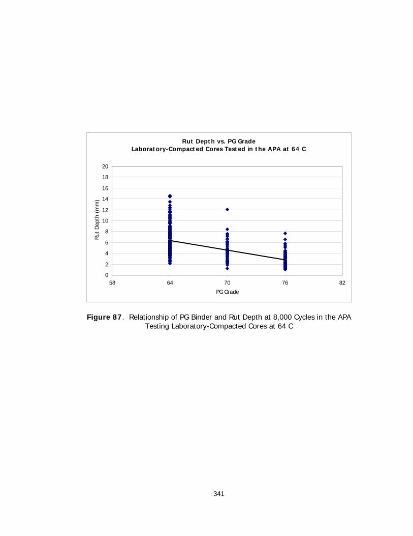
341
Rut Depth vs. PG GradeLaboratory-Compacted Cores Tested in the APA at 64 C
0
2
4
6
8
10
12
14
16
18
20
58 64 70 76 82
PG Grade
Rut
Dep
th (
mm
)
Figure 87. Relationship of PG Binder and Rut Depth at 8,000 Cycles in the APA Testing Laboratory-Compacted Cores at 64 C

342
Rut Depth vs. NMASLaboratory-Compacted Cores Tested in the APA at 64 C
0
2
4
6
8
10
12
14
16
18
20
5.0 7.5 10.0 12.5 15.0 17.5 20.0 22.5 25.0 27.5 30.0 32.5 35.0 37.5 40.0
NMAS
Rut
Dep
th (
mm
)
Figure 88. Relationship of NMAS and Rut Depth at 8,000 Cycles in the APA Testing Laboratory-Compacted Cores at 64 C

APPENDIX A

Mix Design Summary
Highway: Interstate 30 West
Location: Little Rock
Job Number: 060802 Sampling Date:
Nmax: 228 September 1997
Ndes: 139
Nini: 9
Binder Content: 5.5%
PG Grade: 76-22
NMAS: 12.5 mm
Primary Agg. Type: Syenite
Gb: 1.033 Design Gsb: 2.589
Design Air Voids: 4.0% Design Gse: 2.629
Design Gmm: 2.423 % Passing #4: 57
Design VMA: 14.7% % Passing #8: 37
VMA Correction: 1.3% % Passing #200: 3.2
Design VFA: 75.0% % Natural Sand: 0
Design F/A Ratio: 0.65 Gradation Type: BRZ
Marshall Stability: 100.0% Surface Area
(ft2/lb): 20.64
Avg. AASHTO T 283 TSR: 84.2% Percent Insoluble: 100
Film Thickness (µm) 11.9

Design Summary
Highway: Interstate 30 West
Location: Little Rock
Job Number: 060802 Sampling Date:
Nmax: 228 September 1997
Ndes: 139
Nini: 9
Binder Content: 4.2%
PG Grade: 76-22
NMAS: 25.0 mm
Primary Agg. Type: Syenite
Gb: 1.033 Design Gsb: 2.609
Design Air Voids: 4.0% Design Gse: 2.626
Design Gmm: 2.466 % Passing #4: 28
Design VMA: 13.1% % Passing #8: 21
VMA Correction: 0.5% % Passing #200: 3.2
Design VFA: 69.3% % Natural Sand: 0
Design F/A Ratio: 0.81 Gradation Type: BRZ
Marshall Stability: 90.1% Surface Area
(ft2/lb): 17.02
Avg. AASHTO T 283 TSR: 82.7% Percent Insoluble: 100
Film Thickness (µm) 11.5

Design Summary
Highway: Interstate 40
Location: Morgan
Job Number: 060592 Sampling Date:
Nmax: 240 April 1998
Ndes: 146
Nini: 9
Binder Content: 5.2%
PG Grade: 76-22
NMAS: 12.5 mm
Primary Agg. Type: Syenite
Gb: 1.030 Design Gsb: 2.588
Design Air Voids: 4.0% Design Gse: 2.631
Design Gmm: 2.434 % Passing #4: 59
Design VMA: 14.4% % Passing #8: 38
VMA Correction: 1.4% % Passing #200: 4.8
Design VFA: 72.0% % Natural Sand: 0
Design F/A Ratio: 0.72 Gradation Type: BRZ
Marshall Stability: NA Surface Area
(ft2/lb): 25.52
Avg. AASHTO T 283 TSR: 91.0% Percent Insoluble: 100
Film Thickness (µm) 9.0
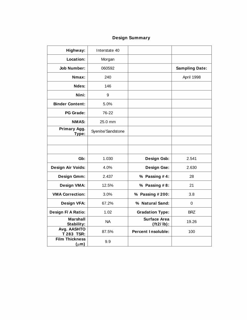
Design Summary
Highway: Interstate 40
Location: Morgan
Job Number: 060592 Sampling Date:
Nmax: 240 April 1998
Ndes: 146
Nini: 9
Binder Content: 5.0%
PG Grade: 76-22
NMAS: 25.0 mm
Primary Agg. Type: Syenite/Sandstone
Gb: 1.030 Design Gsb: 2.541
Design Air Voids: 4.0% Design Gse: 2.630
Design Gmm: 2.437 % Passing #4: 28
Design VMA: 12.5% % Passing #8: 21
VMA Correction: 3.0% % Passing #200: 3.8
Design VFA: 67.2% % Natural Sand: 0
Design F/A Ratio: 1.02 Gradation Type: BRZ
Marshall Stability: NA Surface Area
(ft2/lb): 19.26
Avg. AASHTO T 283 TSR: 87.5% Percent Insoluble: 100
Film Thickness (µm) 9.9

Design Summary
Highway: US Highway 71B
Location: Springdale
Job Number: 040274 Sampling Date:
Nmax: 195 June 1998
Ndes: 121
Nini: 9
Binder Content: 6.2%
PG Grade: 70.22
NMAS: 12.5 mm
Primary Agg. Type: Limestone/Sandstone
Gb: 1.016 Design Gsb: 2.527
Design Air Voids: 4.0% Design Gse: 2.603
Design Gmm: 2.373 % Passing #4: 42
Design VMA: 15.5% % Passing #8: 29
VMA Correction: 2.4% % Passing #200: 3.1
Design VFA: 73.0% % Natural Sand: 0
Design F/A Ratio: 0.62 Gradation Type: BRZ
Marshall Stability: 95.5% Surface Area
(ft2/lb): 17.26
Avg. AASHTO T 283 TSR: 89.0% Percent Insoluble: 100
Film Thickness (µm) 15.1

Design Summary
Highway: Arkansas Hwy. 45
Location: Hartford
Job Number: R40129 Sampling Date:
Nmax: 129 July 1998
Ndes: 83
Nini: 7
Binder Content: 6.3%
PG Grade: 64-22
NMAS: 12.5 mm
Primary Agg. Type: Sandstone
Gb: 1.031 Design Gsb: 2.533
Design Air Voids: 4.0% Design Gse: 2.621
Design Gmm: 2.389 % Passing #4: 54
Design VMA: 15.3% % Passing #8: 29
VMA Correction: 2.8% % Passing #200: 5.8
Design VFA: 73.8% % Natural Sand: 0
Design F/A Ratio: 1.19 Gradation Type: BRZ
Marshall Stability: 81.8% Surface Area
(ft2/lb): 26.50
Avg. AASHTO T 283 TSR: 95.4% Percent Insoluble: 100
Film Thickness (µm) 9.6

Design Summary
Highway: Arkansas Hwy. 22
Location: Dardanelle
Job Number: 080124 Sampling Date:
Nmax: 150 August 1998
Ndes: 95
Nini: 8
Binder Content: 5.8%
PG Grade: 64-22
NMAS: 12.5 mm
Primary Agg. Type: Sandstone
Gb: 1.033 Design Gsb: 2.560
Design Air Voids: 4.0% Design Gse: 2.652
Design Gmm: 2.431 % Passing #4: 60
Design VMA: 14.3 % Passing #8: 36
VMA Correction: 3.0% % Passing #200: 3.2
Design VFA: 72.0% % Natural Sand: 0
Design F/A Ratio: 0.71 Gradation Type: BRZ
Marshall Stability: 90.4% Surface Area
(ft2/lb): 20.14
Avg. AASHTO T 283 TSR: 85.1% Percent Insoluble: 100
Film Thickness (µm) 11.2

APPENDIX B

Standard Test Method for DETERMINING RUTTING AND STRIPPING SUSCEPTIBILITY USING THE
EVALUATOR OF RUTTING AND STRIPPING IN ASPHALT (ERSA)
1. SCOPE
1.1 This method covers the procedure for testing the rutting and stripping susceptibility of hot mix asphalt (HMA) mixtures using the Evaluator of Rutting and Stripping in Asphalt (ERSA).
1.2 The units stated for values are to be regarded as the standard. The values given in parentheses are for information only.
1.3 This standard does not purport to address all of the safety concerns, if any, associated with its use. It is the responsibility of the user of this standard to establish appropriate safety and health practices and to determine the applicability of regulations prior to use.
2. REFERENCED DOCUMENTS 2.1 AASHTO Standards: PP2 Short- and Long-Term Aging of Bituminous Mixes
TP4 Preparation of Compacted Specimens o Modified and Unmodified Hot Mix Asphalt by Means of the SHRP Gyratory Compactor
T166 Bulk Specific Gravity of Compacted Bituminous Mixtures Using Saturated Surface-Dry Specimens
T168 Standard Practice for Sampling Bituminous Paving Mixtures T209 Theoretical Maximum Specific Gravity and Density of Bituminous
Paving Mixtures T269 Percent air Voids in Compacted Dense and Open Bituminous
Paving Mixtures 3. APPARATUS
3.1 Evaluator of Rutting and Stripping in Asphalt (ERSA) – A thermostatically controlled device designed to test the rutting susceptibility of hot mix asphalt by applying repetitive linear loads to compacted test specimens by a steel wheel.
3.1.1 ERSA shall be thermostatically controlled to maintain the test temperature in the testing chamber at any setting between 20 C and 65 C, accurate to 1 C.
3.1.2 ERSA shall be capable of maintaining a constant temperature in two recirculating water baths at settings in the range of 20 C to 65 C, accurate to 1 C. The water recirculation unit shall be capable of continuously monitoring the temperature of the water in the water baths.
3.1.3 ERSA shall be capable of independently applying loads up to 705 N (158 lb) to each wheel. The loads shall be calibrated to the desired test load by a load cell.
3.1.4 ERSA shall contain at least two sample trays and be capable of testing at least two samples simultaneously.
3.1.5 ERSA shall have a master cycle counter.

3.1.6 ERSA shall have an automated data acquisition system for the purpose of collecting cycle number and vertical deformation information for the entire profile of each sample. Rut depth measurements shall be accurate to 0.01 mm.
3.2 Balance, 6,000 gram capacity, accurate to 0.1 gram. 3.3 Mixing utensils (bowls, spoon, spatula) 3.4 Ovens for heating aggregate and asphalt cement. 3.5 Compaction device and molds.
4. PREPARATION OF TEST SPECIMENS
4.1 Number of test specimens – Each ERSA test will consist of four cylindrical specimens (150 mm in diameter), comprising two ERSA samples. Sample height should be at least 75 mm and not more than 175 mm. Samples should be compacted to contain 7.0 ± 1.0 percent air voids.
4.2 Laboratory Prepared Mixtures 4.2.1 Mixture proportions are batched in accordance to the desired Job
Mix Formula. 4.2.2 The asphalt binder and aggregates shall be mixed and compacted
in accordance with AASHTO TP4. 4.2.3 Test samples shall be aged in accordance with the short-term
aging procedure in AASHTO PP2. 4.3 Plant Produced Mixtures
4.3.1 Samples of plant-produced mixtures shall be obtained in accordance with AASHTO T169. Representative samples should be split from the sampled quantity such that the desired sample height will be obtained following specimen compaction.
4.3.2 Specimens shall be compacted in accordance with AASHTO TP4. 5. DETERMINATION OF AIR VOID CONTENT
5.1 Determine the bulk specific gravity of the test specimens in accordance with AASHTO T166.
5.2 Determine the maximum specific gravity of the test mixture in accordance with AASHTO T209.
5.3 Determine the air void content of each test specimen in accordance with AASHTO T269.
5.4 Pair specimens such that two cylindrical specimens will comprise one ERSA test sample.
6. MOLDING SPECIMENS
6.1 Wire the specimens lengthwise to a non-flexible plate, such that the plate will span the length of the sample tray.
6.2 Place acrylic spacer blocks to occupy mold volume not needed for the sample. The spacer blocks should not touch the HMA samples when molded.
6.3 Place HMA sample such that its top surface is flush with the plane of the top of the sample mold.
6.4 Mix plaster of paris according to manufacturer instructions, and fill all voids in the sample mold.

NOTE: A plastic membrane place in the bottom the sample mold may help to prevent leaks.
6.5 Allow the plaster to cure until sufficiently hardened to prevent deformation. 6.6 Remove the lengthwise plate and place molded sample in ERSA.
7. TEST TEMPERATURE, SPEED, AND LOAD
7.1 The test shall be performed at a temperature of 50 C in the submerged condition.
7.2 The wheel speed shall be set such that approximately 550±50 cycles are applied to the sample each hour.
7.3 The load applied to the sample shall be 132 lb (589 N). 8. SPECIMEN PREHEATING
8.1 Samples shall be subjected to a static soak conditioning period in the temperature calibrated ERSA water bath. The conditioning period should last a minimum of four hours and a maximum of eight hours.
9. PROCEDURE
9.1 Apply the 132 lb load to each test sample. 9.2 Provide a unique filename for the file containing sample data. 9.3 Prepare the data acquisition system for the test. 9.4 Apply 10 to 15 cycles to seat the samples prior to the initial deformation
measurement. 9.5 Apply 20,000 cycles to the samples.
10. CALCULATIONS
10.1 Use the average of ten profile points at the interior of each cylindrical specimen making up the test sample as the basis for all calculations. Average rut depth shall be plotted graphically against number of cycles.
10.2 Calculate the rut depth as the difference in the final and initial rut depth measurements, in millimeters.
10.3 Initial consolidation is determined as the depth of compaction experienced by the sample prior to the start of the rutting slope.
10.3.1 Initial consolidation should occur within the first hour of testing. 10.4 The rutting slope is the inverse of the slope of the linear portion of the
rutting response curve, prior to the onset of stripping. 10.4.1 Rutting slope is presented as the number of cycles required to
create a 1-mm rut depth. 10.5 The stripping slope, if present, is the inverse of the slope of the linear
portion of the stripping response curve, after the onset of stripping. 10.5.1 Stripping slope is presented as the number of cycles required to
create a 1-mm rut depth. 10.6 The stripping inflection point, if present, is the point of intersection of the
rutting slope and stripping slope. 10.6.1 Stripping inflection point is presented as the number of cycles
corresponding to the intersection of the rutting and stripping slopes.
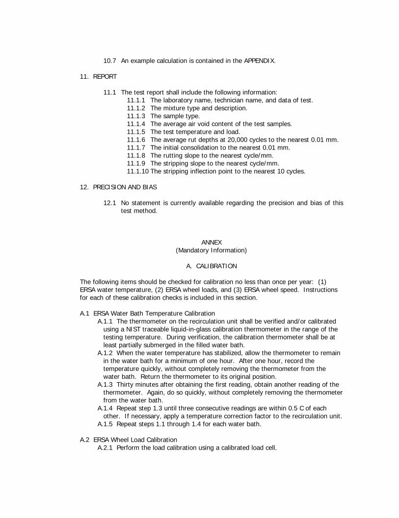
10.7 An example calculation is contained in the APPENDIX. 11. REPORT
11.1 The test report shall include the following information: 11.1.1 The laboratory name, technician name, and data of test. 11.1.2 The mixture type and description. 11.1.3 The sample type. 11.1.4 The average air void content of the test samples. 11.1.5 The test temperature and load. 11.1.6 The average rut depths at 20,000 cycles to the nearest 0.01 mm. 11.1.7 The initial consolidation to the nearest 0.01 mm. 11.1.8 The rutting slope to the nearest cycle/mm. 11.1.9 The stripping slope to the nearest cycle/mm. 11.1.10 The stripping inflection point to the nearest 10 cycles.
12. PRECISION AND BIAS
12.1 No statement is currently available regarding the precision and bias of this test method.
ANNEX (Mandatory Information)
A. CALIBRATION
The following items should be checked for calibration no less than once per year: (1) ERSA water temperature, (2) ERSA wheel loads, and (3) ERSA wheel speed. Instructions for each of these calibration checks is included in this section. A.1 ERSA Water Bath Temperature Calibration
A.1.1 The thermometer on the recirculation unit shall be verified and/or calibrated using a NIST traceable liquid-in-glass calibration thermometer in the range of the testing temperature. During verification, the calibration thermometer shall be at least partially submerged in the filled water bath.
A.1.2 When the water temperature has stabilized, allow the thermometer to remain in the water bath for a minimum of one hour. After one hour, record the temperature quickly, without completely removing the thermometer from the water bath. Return the thermometer to its original position.
A.1.3 Thirty minutes after obtaining the first reading, obtain another reading of the thermometer. Again, do so quickly, without completely removing the thermometer from the water bath.
A.1.4 Repeat step 1.3 until three consecutive readings are within 0.5 C of each other. If necessary, apply a temperature correction factor to the recirculation unit.
A.1.5 Repeat steps 1.1 through 1.4 for each water bath. A.2 ERSA Wheel Load Calibration
A.2.1 Perform the load calibration using a calibrated load cell.

A.2.2 Position the load cell directly beneath the center of the wheel in its lowered position.
A.2.3 Zero the load cell. A.2.4 Lower the wheel and apply the normal testing load. A.2.5 Allow the load cell reading to stabilize. Record the load. A.2.6 Repeat steps 2.2 through 2.5 for each ERSA wheel.
A.3 ERSA Wheel Speed Calibration A.3.1 Using a stopwatch, record the number of wheel cycles completed in one
minute. Multiply this value by 60. If the result is not within the specified tolerance, adjust the speed of the motor.
A.3.2 Repeat this process until three consecutive readings are acceptable.
APPENDIX (Nonmandatory Information)
X1. Calculation of Test Data
X1.1 Inverse of linear slope (cycles/mm) = (C2 – C1) / (R2 – R1) Where C1 = Number of Cycles at Beginning of Linear Portion C2 = Number of Cycles at End of Linear Portion R1 = Rut Depth at Beginning of Linear Portion (mm) R2 = Rut Depth at End of Linear Portion (mm) X1.2 Sample Data Plot
AR22 - Dardanelle - Sample B3 - 2ERSA - 50 C and 132 lb Load - Field Slab
0
24
6
8
1012
14
1618
200 2000 4000 6000 8000 10000 12000 14000 16000 18000 20000 22000
Number of Cycles
Rut D
epth
(mm
)
Rutting Slope
Stripping Slope
SIP


![Empresa Ersa[1]](https://img.dokumen.tips/doc/110x75/55d5763ebb61eb8b0d8b45cb/empresa-ersa1.jpg)