Embed Size (px)
Citation preview

GEOSTATISTICAL ANALYSIS OF A SOILSALINITY DATA SET
G. Bourgault,r A. G. Joumel,’ J. D. Rhoades,z D. L. Cot-win,2 andS. M. Lesch2
iGeological and Environmental Sciences Department,Stanford University, Stanford, California 94305
WSDA-ARS, U.S. Salinity Laboratory,450 Big Springs Road, Riverside, California 92507
I. IntroductionA. Broadview Salinity Data Set
II. Exploratory Data AnalysisA. Electrical Conductivity DataB. Electromagnetic DataC. Soil Type DifferentiationD. Spatial and Variogram Analysis
III. Mapping the EC, DistributionA. Comments on ResultsB. Influence of EMi, Data
IV. Filtering StructuresV Spatial Cluster Analysis
VI. Stochastic ImagingA. Simulation Algorithm
VII. Assessment of Spatial UncertaintyVIII. Ranking of Stochastic Images
IX. ConclusionsReferences
I. INTRODUCTION
Rather than relating a specific case study with specific goals, this study aims atpresenting a range of potential applications of modem geostatistics to soil surveyproblems using a real data set. Typical of the development of geostatistics, adiscipline led by engineers, many new algorithms, although well published in
241
Advances in Agronomy, Volume 58Copyright 6 1997 by Academic Press, Inc. All rights of reproduction in any form reserved.

242 G. BOURGAULT ET AL.
their field of inception (mining and petroleum), have not yet found their way intomainline statistical books; hence, they may not be readily accessible to profes-sionals outside the extractive industry (Deutsch and Joumel, 1992; Dimit-rakopoulos, 1993; Isaaks and Srivastava, 1989; Soares, 1993). It is hoped thatthis presentation may raise enough interest among soil scientists so that they findit worth their time to learn more about modem geostatistical concepts of dataanalysis, estimation, uncertainty assessment, and stochastic imaging. All resultspresented in this study were obtained using standard mapping routines and thepublic-domain GSLIB software (Deutsch and Joumel, 1992). FORTRAN sourcecode of the latter is public domain; hence, it is available to whomever wishes tounderstand the details of any particular algorithm and/or to modify it to fit anyparticular problem at hand.
A common denominator of many soil sciences data sets is the sparsity of“hard” or direct measurements of the primary variable of interest, usually bal-anced by the prevalence of “soft” or indirect information related to the primaryvariable. Examples of hard data are core measurements and more generally ex-pensive field-based data as opposed to soft data obtained, e.g., from remotesensors. Geographical information systems (GIS) and geostatistics pursue a simi-lar objective-that of providing tools for the integration of different objectives,and that of providing tools for the integration of different information sourceswith varying relevance/reliability to build maps that summarize and expand theoriginal hard data set. Geostatistics propose to add to the GIS toolbox variousspatial data analysis tools to explore and model patterns of space/time depen-dence between the data available. The resulting numerical models, e.g., vario-grams or conditional distributions, can then be put to use for various mappingpurposes and an assessment of the reliability of such maps.
Just as there is no unique or optimal sequence in using GIS tools, such asconcatenation, intersection, or interpolation, there is no unique geostatisticalapproach to spatially distributed data. Many alternative covariance/variogrammodels can be fitted to the same data set depending on ancillary informationavailable to the operator (including his or her own prior experience); there aremany different kriging algorithms (generalized least squares regression) that canbe used toward the same mapping goal depending on which particular aspect ofthe data one wishes to capitalize on. What may be lost to statistical objectivity(an extremely debatable concept) is gained in flexibility and ability to handlesoft, yet essential information of various types. It is better to have a somewhatsubjective but accurate assessment that accounts for all relevant information thana supposedly objective assessment that misses critical aspects of the problem.This chapter will illustrate the toolbox aspect of geostatistics, presenting severalalternative ways to reach the same goal and proposing cross-validation exercisesto help the operator in his or her decision.

GEOSTATISTICAL ANALYSIS OF A SOIL SALINITY DATA SET 243
A. BROADVIEW SALINITY DATA SET
As mentioned previously, the data set used in the following study is more asupport for demonstration of geostatistical algorithms than the data base of anactual case study. For such demonstrative purposes, the name of the locationinvolved and even the measurement units of the data could have been omitted,and coordinate values could have been changed by any one-to-one monotonictransform leaving unchanged the relative patterns of spatial variability of thevarious attributes.
The actual and complete Broadview salinity data base and its statistical analy-sis are presented in various papers and reports of the U.S. Salinity Laboratory(Lesch et al., 1995a,b). The reader is referred to these papers for any questionrelated to sampling and salinity assessment in the Broadview water district. Theresults of the present study are based on a limited data set ignoring, in particular,such critical variable as soil water saturation: they should only be used to assessthe worth of adding geostatistical tools to GIS and other toolboxes available tothe soil scientist.
The Broadview data set covers approximately 6 0 0 0 acres and comprises thefollowing:
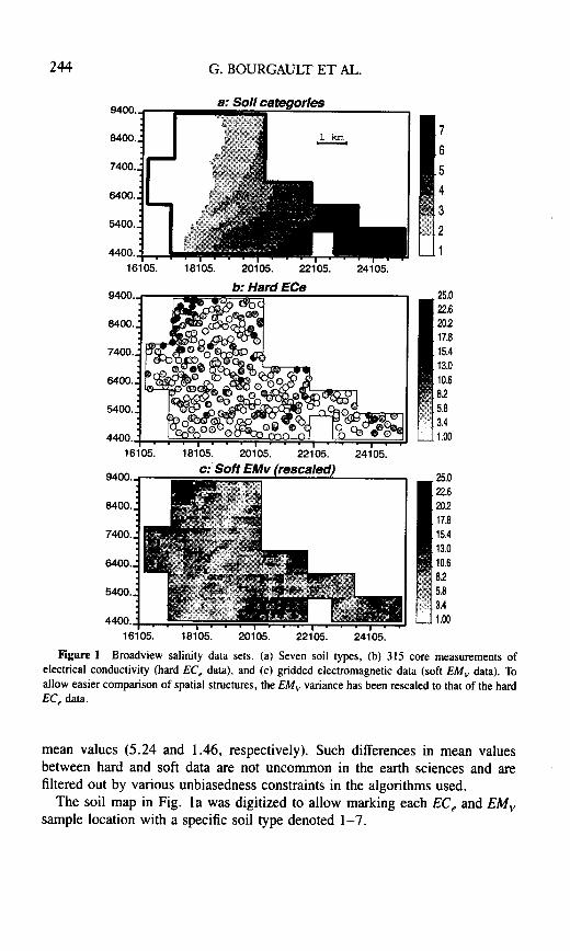
l a soil map digitized into 7 soil types (see Fig. la).l 315 soil core measurements of electrical conductivity (EC,), taken at four
depths (O-l, 1-2, 2-3, and 3-4 ft) (see Fig. lb). Unit is dS/m.l 2385 measurements of soil vertical (EM,) and horizontal (EM,) electromag-
netic response (see Fig. lc). Unit is dS/m. Each measurement is deemedrepresentative of the vadose zone (upper 4 ft of soil). The extent of thatelectromagnetic information delineates the study area, as shown in Figs. la-1c.
For the purpose of this study, core EC, values are considered hard data directlyrelated to soil salinity and represent the primary variable to be evaluated through-out the vadose zone. The electromagnetic induction readings represent a second-ary variable less directly related to soil salinity; they are considered soft data usedto complement the hard EC, data. With little loss of location accuracy, electro-magnetic data have been relocated to the nodes of a 2D regular grid 100 X 100m. The few grid nodes with no electromagnetic sample within a radius of 50 mwere left uninformed. Another option could have been to interpolate the fewmissing nodal values. The grid includes 2385 EM, measurements. To allowstandardization of the grayscales, the EM, data plotted in Fig. lc have beenrescaled by a factor equal to the ratio of the standard deviations of original EC,and EM, data.
Although measured in the same unit (dS/m), EC, and EM, data have different
GEOSTATISTICAL ANALYSIS OF A SOIL SALINITY DATA SET 245
II. EXPLORATORY DATA ANALYSIS
The aim of an exploratory data analysis (EDA) is to acquire an overall famil-iarity with the data, their interrelations, statistical grouping, spatial distribution,clustering, etc. At this stage, the operator should not be constrained by anyspecific goal but rather he or she should be attentive to any clue the data may givethat may prove useful in later interpretations. Because geostatistics deals withspatial data, extensive use should be made of isopleth maps and GIS-relatedroutines depicting the relations between data values and their space/time coordi-nates. Beware that random sampling (random drawing of sample coordinates)does not make the data values independent inasmuch as it is the physical generat-ing process that makes the data dependent and not the human decision aboutwhere samples are taken.
A. ELECTRICAL CONDUCTIVITY DATA
Figure 2 shows the succession of four grayscale EC, maps corresponding tothe four measurement depths. The vertically averaged map is that shown in Fig.lb. There appears to be a gradual increase in soil salinity with depth, corrobo-rated by the histograms shown on the right in Fig. 2.
A diagonal transect Nl20”E crosscutting the N30“E elongation of the sevensoil categories shown in Fig. la was defined, then EC, data values were plottedagainst their coordinate value along that transect (see Fig. 3). At each depthlevel, the n = 315 EC, data were ranked from r(i) = 1 to rC@ = 315 and theirstandardized ranks v(i) = fii)ln, or uniform scores distributed in [0,l], are gray-scale plotted in Fig. 3. This uniform score transform allows identifying eachlevel-specific EC, data set to the same uniform [O,l] distribution. This transformthus filters out the vertical trend previously observed and allows comparison ofthe strictly horizontal structures. The four Nl20”E grayscale transects of uniformscores shown on the left in Fig. 3 show similarity of the horizontal variability ofEC, data over the four depth levels. This is confirmed by the EC, uniform score(uscore) semivariograms calculated along the N120”E direction and given on theright in Fig. 3. Therefore, these uscores-standardized variograms can be pooledtogether into a single model valid for all four depth levels.
The rank (or uscores) correlations between two vertically consecutive EC, data(thus with the same horizontal coordinates) are 0.64 for l-2 ft, 0.80 for 2-3 ft,and 0.89 for 3-4 ft. Therefore, except for the first transition from 1 to 2 ft, theEC, data are quite redundant from one level to the next one: there is little gain tobe expected from a 3D interpolation versus a much simpler 2D exercise usingonly data from the level being estimated.


248 G. BOURGAULT ET AL.
For the remainder of that study and for reason of conciseness, only the ver-tically averaged EC, data (see Fig. 1 b) were considered together with the corre-sponding 2D-distributed electromagnetic data (see Fig. lc).
Note that the uniform score transform x -+ F,(x), where F,(a) is the cumula-tive distribution function (cdf) of random variable X, is the first step of a normalscore transform (Deutsch and Joumel, 1992, p. 138). Unless properties specificto the Gaussian distribution are to be called for, there is no need for going beyondthe standardized rank transform F,(a). This rank transform, by definition, pre-serves the rank of the data as does the commonly used, albeit somewhat arbitrary,log transform. From the histograms of Fig. 2, the EC, data appear neither nor-mal nor lognormal distributed; this was confirmed by probability graph plots(Deutsch and Joumel, 1992, p. 201) not shown here.
B. ELECTROMAGNETIC DATA
Figure 4a shows an extreme redundancy between the two secondary data,vertical (EM,) and horizontal (EM,) electromagnetic measurements. This redun-dancy was confirmed by maps and variograms analysis (not shown here). Be-cause EM, has slightly better correlation with colocated vertically averaged EC,(see Figs. 4b and 4c), only EM, was retained as a source of secondary data forthe rest of the study. The grayscale map of this EM, data was shown in Fig. lc.
Observe on Fig. 4b the nonlinear relation EC,-EM, To linearize that relationand capitalize on linear regression tools (such as kriging), a transform of thevariables is necessary. If the two variables were to be made Gaussian distributed,a normal score transform (Isaaks and Srivastava, 1989, p. 138) would be neces-sary. Because the histograms of the original EC, and EM, values are not lognor-mal, the log transform does not identify the normal score transform. In any case,there is currently no need for any Gaussian assumption; hence, the rank trans-form (uniform scores) is enough.
Figure 4d shows the scattergram of the uniform score transforms of EC, andEM, data. Note how the rank transform has succeeded in linearizing the originalregression between EC, and EM, data (see Fig. 4b). The linear rank regressionremains though heteroscedastic, in the sense that higher ranks of EC, are betterpredicted by corresponding high EM, ranks than are lower ranks. These rankregressions will be fine-tuned later using soil type information.
C. SOIL TYPE DIFFERENTIATION
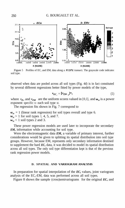
The 3 15 vertically averaged EC, data values were plotted against their coordi-nates along the N120”E transect and grayscale coded for soil type (see Fig. 5a).Figure 5b provides a similar profile for the 2385 EM, data.

GEOSTATISTICAL ANALYSIS OF A SOIL SALINITY DATA SET 249
3.0 a: EMh - EMv
2.5
c: ECe - EMh .21.3 . Number of data 315
x variable: m ean1 .01std. dev.. 0.40
Y Variable: mean 5.2416.3 std. dev. 3.32.
* correlationa. rank correlation
8 .70.66. _
EMh
25.0 b: ECe-EMvNumber of data 315
. x Variable: mean 1 . 4 7.
20.01std. dev. 0.52
V Variable: mean 5.24std. dev. 3.32
EMv
d : Uscores ECe-EMv _
0.0 -... - _ . . .
02 012 014 016 016
uscEMv
Figure 4 Scattergrams. (a) Soft EM, versus soft EM, data; (b) hard EC, versus soft EM, data;(c) hard EC, versus soft EM, data; and (d) uniform scores of ECe versus EMv data.
Except for soil types 1 and 6 (the latter being nonrepresentative because oflack of data), the ranges of EC, values appear homogeneous across soil types.This is confirmed by the EC, histograms per soil type (not shown).
The histograms of EMI, data per soil type (Fig. 6) would lead one to differenti-ate the following two groups based on mean EM, value:
l A first group including soil types 1, 4, 5, and 7 with a mean EM, valuearound 1.6
l A second group including soil types 2, 3, and 6 with a lower mean EM,value around 1.2
Note that these two groups are intermingled in space.EM, data considered to be exhaustively sampled, are used to inform un-
sampled primary EC, values. To investigate how soil type influences the relation,EC,-EM, the seven soil-specific rank scattergrams of uscores of colocated EC,and EM, data are shown in Fig. 7. It appears that the linear rank regression
250 G. BOURGAULT ET AL.
25.0a: ECe
J 00
20.0
O.O’.,. ,.. .,. ,., ..r14000. 16000 18000 20000 22000 24000
X (N120E)
b: EMv
0.00 1 . . . .14000 1 6 0 0 0 1 8 0 0 0 20000 22000 24
X (N120E)
I.
Figure 5 Profiles of EC, and EM, data along a N120”E transect. The grayscale code indicatessoil type.
observed when data are pooled across all soil types (Fig. 4d) is in fact constitutedby several different regressions better fitted by power models of the type,
vEc< = ]VEM J”n (1)where v,, and vemv, are the uniform scores valued in [0,l], and o,, is a powerexponent specific t o each soil type st.
The regression fits shown in Fig. 7 correspond to
US, = 1 (linear rank regression) for soil types overall and type 6.o,, > 1 for soil types 1, 4, 5, and 7.w,, < 1 soil types 2 and 3.
These power regression models are used later to incorporate the secondaryEM, information while accounting for soil type.
Were the electromagnetic data EM, a variable of primary interest, furtherconsiderations would be given to splitting its spatial distribution into soil typegroups. However, because EM, represents only secondary information destinedto supplement the hard EC, data, it was decided to model its spatial distributionacross all soil types. The only soil type differentiation kept is that of the previousrank regression power models.
D. SPATIAL AND VARIOGRAM ANALYSIS
In preparation for spatial interpolation of the EC, values, joint variogramanalysis of the EC,-EM, data was performed across all soil types.
Figure 8 shows the sample (cross)semivariograms for the original EC, and


254 G. BOURGAULT ET AL.
The solid lines in Fig. 8 show the fit by a model of coregionalization (Joumeland Huijbregts, 1978, p. 172; Isaaks and Srivastava, 1989, p. 390). That modelfeatures
l An isotropic nugget effect accounting for about one-third of the total spatialvariance of the EC, data
l A first isotropic structure of range 700 m accounting for another third of theEC, variance
l A second anisotropic structure of range 3000 m in the N120”E directionacross soil types and 16,000 m in the N3o”E direction along soil continuity
The model for EM, is similar although with lesser nugget effect due to thelarger definition volume (averaging effect) of the electromagnetic data.
The original EC, and EM, data were then normal score transformed (Deutschand Joumel, 1992, p. 138) so that both histograms identify a standard Gaussiandistribution, and the corresponding sample (cross)semivariograms were calcu-lated and modeled (see Fig. 9). The coregionalization model features the samecharacteristics as those fitted to the original data. Note that sampling fluctuationshave not been significantly reduced by the normal score transform; this wouldhave also been true had a log-transform been used.
The uniform scores of the EM, and EC, data used are shown in Figs. 10a andl0b. Compare these scores to the data in Fig;. lc and lb, respectively: except forthe different grayscales, they are essentially the same. Again, we prefer compar-ing data through the uniform standardization in [0,l] provided by the stan-dardized ranks (uniform scores). Figure 1Oc shows the location of 26 EC, ran-dom samples taken from the 3 15 original EC, data; this subsample is used later inthe cross-validation exercises.
III. MAPPING THE EC, DISTRIBUTION
To demonstrate the various geostatistical mapping algorithms, four differentapproaches and two sampling cases are considered. EC, estimation is performedat each node of the 100 X 100-m grid covering the study area as defined by thetemplate of electromagnetic data (see Fig. lc).
The three different approaches are
1. Simple kriging (SK) (Deutsch and Joumel, 1992, p. 62): EC, is estimatedby a linear combination of the neighboring EC, data plus the overall EC, samplemean, m = 5.24. No secondary information is used; thus, this approach repre-sents a base case.
2. Simple cokriging (coSK) (Deutsch and Joumel, 1992, p. 71): EC, is esti-


GEOSTATISTICAL ANALYSIS OF A SOIL SALINITY DATA SET 257
value is Gaussian with mean and variance identified to the simple kriging meanand variance. The Gaussian conditional cumulative distribution function ( c d f )can be denoted by
Prob {Y(u) : y ( neighboring y(u,) data} = G Y - YS*K(U)o,,(u) > (2)
where Y(u) is the normal score transform of EC, at grid location u, y&(u) andc&(u) are the simple kriging estimate and variance using neighboring normalscore EC, data (v(u,)); and the function G(e) is the standard normal cdf.
Let q(u;p) be the corresponding conditional quantile function or inverse of theprevious conditional cdf:
q(u; p) such that G ‘(” “,’ ju;IK(‘) = p E [O, 1]. (3)SK
Srivastava’s p-field approach (Srivastava, 1992) consists of simulating ap-field, that is, a set of spatially correlated uniformly distributed p,(u) values,then transforming them through the previous quantile function into simulatednormal score values JJ,~(u) for EC,:
Y,(U> = q(w,w) (4)
Because there may be several realizations (outcomes) for p,(u) at any locationu, there may be several “simulated” realizations y,(u), hence the subscript nota-tion s for simulation.
The variant proposed here consists of determining, at each location u, a singlevalue p(u) resulting in a single estimate y*(u) for the EC, normal score value:
y*w = qWW) (5)
with P(U) = bE,,,,,(u)Iw3,, as given by the power model in Eq. [I], and st is thesoil type prevailing at location u.
In words, the p-field value to be plugged into the conditional quantile functionq(u;p) is the p value obtained by the regression model [Eq. (1) and Fig. (7)]specific to the soil type prevailing at u and to the uniform score vEMV (II) of theelectromagnetic datum at u.
This p-field approach requires the Gaussian random function model to deter-mine the conditional cdf Eq. (2) from the only two parameters, mean and vari-ance, provided by simple kriging.
A final step back-transforms the normal score estimate y*(u) into EC, esti-mates expressed in the original EC, units.
Note : The three different approaches proposed here to interpolate EC, valuesdo not cover the range of different geostatistical algorithms that could be used for

258 G. BOURGAULT ET AL.
this purpose. The first two approaches proposed are the most straightforward andare likely to be familiar to many readers. The latter approach is a bit more in-volved; it is intended to give the reader a glimpse of the forefront of appliedgeostatistics in which new variants are constantly proposed to better match theproblem at hand and the specific data available.
For each of the previous three approaches, two sampling cases are considered:
1. All 315 hard EC, data are used together with the (exhaustive) EM” and soiltype information present at all nodes being estimated
2. A subsample of only 26 hard EC, data is used (see Fig. 10c) in addition tothe previous EM, and soil type information
This latter sampling case allows a model-validation exercise using the remain-der 289 hard EC, data. The problem with using such a small sample size (26) isthe difficulty of doing any reliable statistical inference. We have decided to setapart the two problems of statistical inference and model validation of the estima-tion approaches proposed. More precisely, for the latter sampling case, althoughonly 26 EC, data were retained for the various krigings, the statistics needed(histogram, variograms, and regression) are those established using all 3 15 harddata, i.e., the same statistics used for the first sampling case. This decisioncorresponds to the extractive industry practice of borrowing statistics from asimilar and better sampled field but using only field-specific data for local estima-tion.
The objective of this specific model validation exercise is twofold:
1. Observe the performance of each model or algorithm under data sparsity2. Evaluate the worth of the secondary information (EM,) under the same
conditions of data sparsity
Three approaches times two sampling cases result in six sets of results. Eachset of results given hereafter includes
l An estimated EC, map in the original EC’, unit.l The corresponding estimated EC, uniform score map, unit free and valued in[0, 1]. These uniform scores are the standardized ranks of the previous EC,estimates. Again, this standardization allows a visual comparison that is unitfree and free of color or grayscale effect.
l The semivariograms of the EC, estimated values plotted against the modelfitted to the (3 15) sample semivariograms. That model is the one depicted bythe continuous curves in the two top graphs in Fig. 8. This comparisonallows for the evaluation of the smoothing effect (Deutsch and Joumel,1992, pp. 17, 61) of the estimation algorithm considered.
l For the three sets of results corresponding to the second sampling case, the

GEOSTATISTICAL ANALYSIS OF A SOIL SALINITY DATA SET 259
Table 1
Summary of Result.@
Full sample (315) Crow. sample (289)
In uz m crz
Reference 5.24 11.00 5.30 11.02Simple kriging 5.15 4.54 5.34 (p = 0.21) 0.49Simple cokriging 5.21 8.29 5.43 (p = 0.76) 8.45P-field 5.31 13.32 5.57 (p = 0.75) 13.03
u The first two columns give the mean and variance of EC, estimates to be compared to thereference EC, sample used (size 315). The third and fourth columns give the mean and variance of289 reestimated EC, values and their linear correlation with the 289 actual values. For the latter, theEC, subsample size is 26.
cross-validation scattergram of the 289 “true” EC, values versus the corre-sponding estimated values
Table I provides a summary of the major results.
A. COMMENTS ON RESULTS
1. Simple Kriging
The results of the base case, simple kriging using only the full sample of hardEC, data (3 15), are shown in Fig. 11. The grayscale map of the EC, estimates(top map) reveals a severe smoothing effect: the variance of the estimates is only4.54 versus the 315 hard data variance of 11.00. This smoothing effect is a well-known shortcoming of all linear weighted average-type estimators includingkriging (Joumel and Huijbregts, 1978, p. 450): typically, the distribution ofestimates understates the actual proportions of extreme values, whether high orlow values. If detection of spatial patterns of extreme values is the goal of thestudy, then kriging is not an appropriate mapping algorithm (Joumel and Alabert,1988). Instead, one should consider one of the stochastic imaging algorithms,also known as conditional simulations (Deutsch and Joumel, 1992, p. 117),which aim to reproduce the patterns of spatial variability seen from the sampleand modeled through the variogram. Conditional simulations are the topic of thelatter part of this chapter (see Section VII).
The uniform score transform (middle map in Fig. 11) filters the effect ofsmoothing on the global variance and reveals N3O”E structures clearly associated

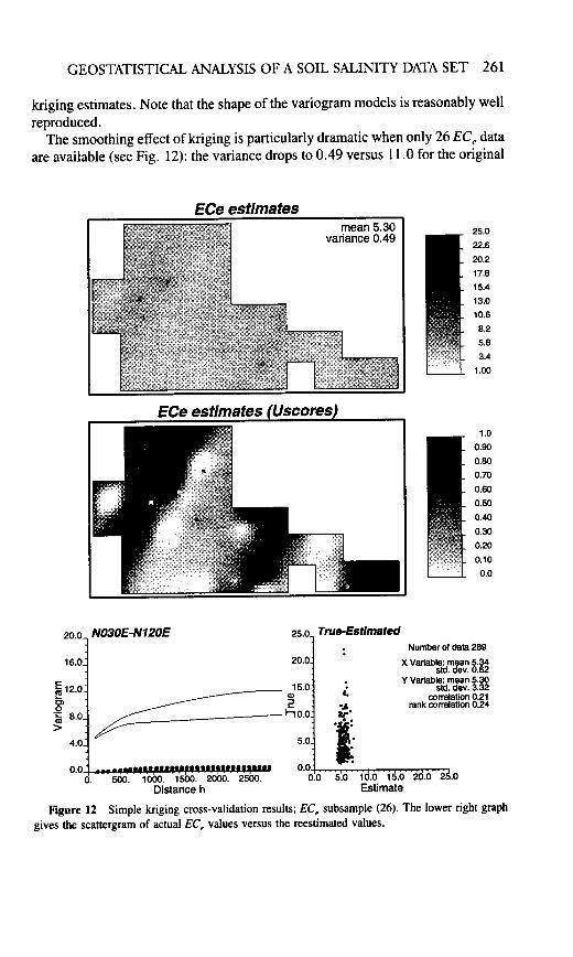

262 G. BOURGAULT ET AL.
sample data. Although globally unbiased, the distribution of the 289 reestimatedvalues fails badly in reflecting the actual proportions of nonmedian EC, datavalues outside the interval [4.0, 8.0] (see scattergram at the lower right in Fig.12). This is known, in geostatistical jargon, as conditional bias (Joumel andHuijbregts, 1978, p. 458).
2. Simple Cokriging
When using the densely sampled secondary (EM,) information, the smoothingof the EC, estimates is partially corrected to 8.29, a value still less than theoriginal sample variance of 11 .OO. The variograms of the cokriging estimatesapproach those of the model much better. The spatial structures of the cokrigingestimates closely reproduce those of the EM, data (compare the uscores maps ofFigs. 13 and 10a); this is as expected given the large EM, sample size and therelatively strong correlation (0.73) between colocated EC, and EM, data (seeFig. 4b).
The contribution of the dense EM, secondary information is more dramaticwhen only 26 hard EC, data are available (compare Figs. 12 and 14). Thescattergram of true versus reestimated EC, values (lower right graph in Fig. 14)indicates a substantial correction of the smoothing effect and related conditionalbias of the simple kriging estimates. In this cross-validation exercise, cokriging(using the secondary information) has raised the true-versus-estimate correlationfrom a low 0.21 to a reasonable 0.76.
3. P-Field Estimates
In addition to the secondary EM, data, the p-field approach implemented hereaccounts for the soil type information.
From the results of Fig. 15, it appears that the smoothing effect seen on thesimple kriging and cokriging estimates in Figs. 11 and 13 has been overcor-rected. The variance of the p-field estimates, 13.30, is now larger than that of theoriginal EC, sample values, 11 .OO; the overcorrection takes place in the N120“Edirection across soil continuity (see the lower right variograms in Fig. 15). Thesoil type information appears to have imposed too much of the soil discontinuityalong that direction.
The cross-validation results of Fig. 16 confirm the correction of the smoothingeffect: the variogram model is well reproduced in both N3O"E and N120”Edirections. The correlation true-versus-reestimated values is not significantlyimproved from the results of cokriging (Fig. 14). Note that the two dots departingmost from the 45” line of the scattergram in Fig. 16 are the same as those in Figs.12 and 14: no estimation algorithm can improve the estimation of outlier values,i.e., values departing significantly from the statistics of the data used. At best,


GEOSTATISTICAL ANALYSIS OF A SOIL SALINITY DATA SET 267
B. INFLUENCE OF EMv DATA
In the two latter estimation algorithms, the sheer density of soft information(one EM, datum at each location being estimated) coupled with the good EC,-EM, correlation (0.73) tend to overwhelm the few hard data available. Oneshould then wonder how much of the structures seen on the EC, estimated mapsin Figs. 13 and 15 pertain to EC, and how much is mere EM, import.
Figure 17 recalls the sample EC,-EM, scattergram as given in Fig. 4b, thengives the four scattergrams of EC, estimates versus colocated EM, values. Thecorrelation EC,-EM, is lowest (0.59) for simple kriging estimates, as expected.Accounting for EM, data increases that correlation to a level (0.86, 0.90) higherthan that of the original sample (0.73). This higher correlation indicates thatindeed there may be too much import of the EM, structures into the EC, mappingexercise. Note that the cokriging estimates show a linear relationship whenplotted against the secondary EM, data (Fig. 17c). The p-field estimates (Fig.17d) reproduce better the nonlinear relationship seen in the sample EC,-EM,scattergram (Fig. 17a).
At the limit, one may think of forfeiting altogether the EC, data and use theEM, map after proper rescaling to identify the sample EC, histogram (Joumeland Xu, 1994). The geostatistical toolbox offers one such algorithm that allowstransforming any data set, e.g., the grid of EM, values, with any given histo-gram H, into another set of values identifying a target histogram H,, with H,possibly quite different from H, . In addition to approximating the target histo-gram, this algorithm allows reproducing (freezing) a few original data values attheir specific locations. This algorithm is a generalization of the well-knownnormal score transform whose target histogram is the standard Gaussian distribu-tion (Deutsch and Joumel, 1992, p. 138).
Figure 18a shows the histogram of the 315 EC, data (the target histogram).Figure 18b shows the histogram of the 2385 EM, data transformed to match thetarget histogram: note the excellent histogram reproduction. These transformedEM, data, expressed in EC, units, are taken as estimates of EC, with their mapshown in Fig. 18c. Per definition of the transformation algorithm, the uscores ofthese EC, estimates identify exactly the EM, uscores (Fig. 10a). Figure 18eshows the scattergram of EC, estimates (actually transformed EM, values) ver-sus the original EM, values: this scattergram has a rank correlation 1 .OO reflect-ing the rank-preserving algorithm underlying the transform used. Recalling thescattergrams of Fig. 17, we have, indeed, gone all the way into importing allEM, structures into the EC, mapping exercise. This time, although there is agood linear correlation coefficient of 0.89 between the EC, estimates (EM,transformed) and the EM, data, the nonlinear relationship EC,-EM, is over-reproduced (cf. Figs. 18e and 17a). The EC, variogram model shape is not


270 G. BOURGAULT ET AL.
This model includes a large nugget effect, a first isotropic structure with range of700 m, and a second anisotropic structure with long range of 16,000 m in theN30”E direction of soil continuity and short range of 3000 m in the N120”Edirection across continuity. The factorial kriging algorithm (Deutsch and Joumel,1992, p. 68) allows filtering out from the simple kriging estimated map at the topof Fig. 11 (reproduced in Fig. 19a) the influence of both nugget effect and short-scale (700 m) structure, leaving the large-scale anisotropic structures (see Fig.19b). Alternatively, one can filter out the influence of the large-scale variogramcomponent leaving the short-scale structure (see Fig. 19c). The “sum” of Figs.19b and 19c plus the nugget effect values at sample locations (not shown) add upto the original simple kriging map of Fig. 19a.
Because the nugget effect and short-scale structure account for such a largeproportion of the EC, spatial variance, the impact of the previous filtering isbetter seen on the corresponding uscore maps (see Fig. 20). Recall that theuniform score transform standardizes all distributions (hence variances) to auniform distribution in [0,l].
Figures 19b and 20b depict the clear anisotropy of the large-scale structureassociated to the soil type distribution (cf. Fig. la). Conversely, Figs. 19c and2Oc zoom on shorter scale patterns of soil salinity possibly related to humanactivities: note the appearance of 1 X l-km quadrats delineating different soilusage (Lesch et al., 1995b). Recall that these maps are based on simple krig-ing-that is, ignoring the EM, information.
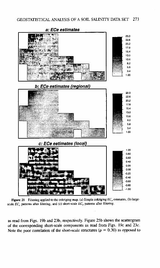
Instead of being integrated in the simple kriging system (Deutsch and Joumel,1992, p. 68), the factorial kriging algorithm can be used on any already availablemap such as the cokriging EC, map shown at the top of Fig. 13. Figures 2 1 and22 give for simple cokriging the same series of maps as given in Figs. 19 and 20for simple kriging, the difference being utilization of the secondary EM, infor-mation. As noted in the previous section, accounting for the dense EM" informa-tion adds considerable local resolution to the estimated EC, maps (cf. Figs. 21aand 19a).
After filtering, the EC, cokriging maps (Figs. 21b and 22b) depict the samelarge-scale structure (related to soil type) seen on the filtered simple kriging maps(Figs. 19b and 20b). However, the short-scales structures seen on the cokrigingmaps (Figs. 21c and 22c) differ markedly from those seen on the simple krigingmaps (Figs. 19c and 20c). To further investigate that difference in short-scalestructures, the EM, data rescaled to the EC, variance 11 .O were directly filtered(see Figs. 23 and 24, whose layouts are the same as those in Figs. 21 and 22). Itappears that the large-scale structure of the EM, data is indeed similar to thatobserved on both the simple kriging and the cokriging EC, estimates (cf. Figs.23b and 24b to Figs. 19b and 20b and to Figs. 21b and 22b). However, the short-scale structures of the EM, data (Figs. 23c and 24c) are clearly different fromthose of the simple kriging EC, estimates (Figs. 19c and 20c). The short-scaleEM, structures reveal a NS-EW lattice possibly linked to the layout of the


GEOSTATISTICAL ANALYSIS OF A SOIL SALINITY DATA SET 279
K X K standardized (cross)covariance functions pkk, (h) between any two RV’sZ,Ju) and Zk,(u + h) separated by vector h. h, = ui - ui is the vector separatingthe two samples i, j at locations ui, uj. Typically, the (K X K) weight matrix[okk,] is identified to the Mahalanobis distance: [ok,‘] = 2-t.
Spatial continuity, anisotropy, and cross-correlation are accounted for throughthe term r(h$ in the definition [Eq. (6)] of the similarity measure S,. Clusteranalysis using this measure will result in grouping of samples with similarattribute values (term sij) but also spatially close together [term r(h$].
The spatial cluster analysis algorithm is demonstrated using only the twodensely sampled electromagnetic attributes, EM, and EM,. No soil data wereused in order to check that cluster analysis using only electromagnetic data doesresult in groups consistent with soil type differentiation.
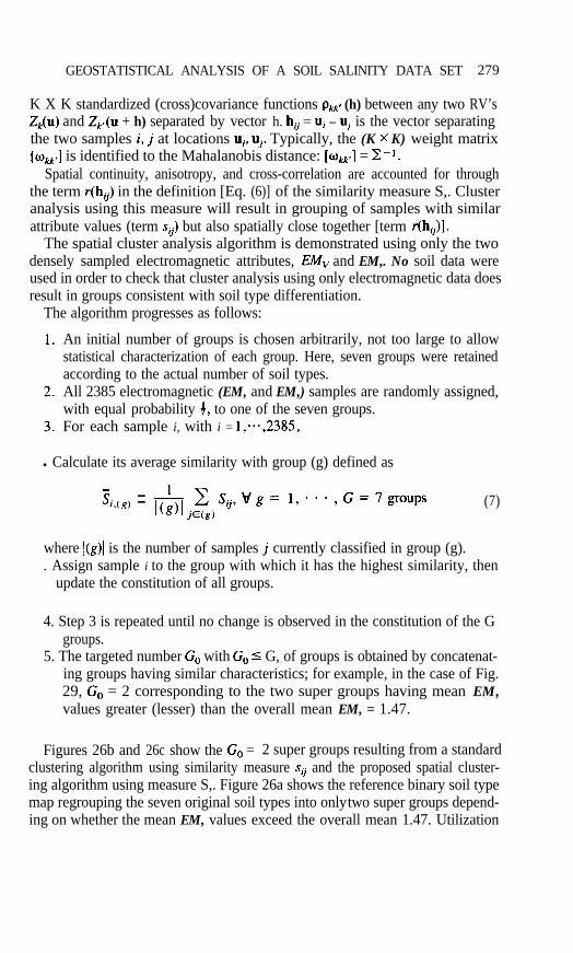
The algorithm progresses as follows:
An initial number of groups is chosen arbitrarily, not too large to allowstatistical characterization of each group. Here, seven groups were retainedaccording to the actual number of soil types.All 2385 electromagnetic (EM, and EM,) samples are randomly assigned,with equal probability f, to one of the seven groups.For each sample i, with i = 1;.*,2385,
l Calculate its average similarity with group (g) defined as
%,(g) = &,c S,,Vg= l;**,G=7groups (7)I%?)
where l(g)1 is the number of samples j currently classified in group (g).. Assign sample i to the group with which it has the highest similarity, then
update the constitution of all groups.
4. Step 3 is repeated until no change is observed in the constitution of the Ggroups.
5. The targeted number G, with G, d G, of groups is obtained by concatenat-ing groups having similar characteristics; for example, in the case of Fig.29, G, = 2 corresponding to the two super groups having mean EM,values greater (lesser) than the overall mean EM, = 1.47.
Figures 26b and 26c show the GO = 2 super groups resulting from a standardclustering algorithm using similarity measure sii and the proposed spatial cluster-ing algorithm using measure S,. Figure 26a shows the reference binary soil typemap regrouping the seven original soil types into only two super groups depend-ing on whether the mean EM, values exceed the overall mean 1.47. Utilization

280 G. BOURGAULT ET AL.
of spatial information results in a much cleaner image closer to the referenceimage obtained from soil type data.
VI. STOCHASTIC IMAGING
In the previous sections, various estimated EC, maps have been presented buttheir accuracy was not assessed. As opposed to mere interpolation algorithms,the main contribution of a geostatistical approach is to provide an assessment ofthe reliability of any given estimated value. What is the reliability of the EC,estimated value at any specific location u? What is the reliability of any clusterof, e.g., high EC, estimated values as seen on the estimated map of Fig. 13? Canthere be alternative estimated maps using the same information?
Besides the kriging estimated value, the solution of any kriging system yieldsa kriging variance-that is, the minimized error variance (Isaaks and Srivastava,1989, p. 286). Unfortunately, because this kriging variance is data values inde-pendent, it is a poor measure of estimation accuracy; instead, it is only a rankingindex of data configuration-the data configuration corresponding to a lesserkriging variance would yield on average (over all possible data values for thatconfiguration) a more accurate estimate.
Even if the kriging variance ai(u) was a measure of accuracy of the estimatedEC, value at location u, the two kriging variances a&(u) and ai would notprovide assessment of joint accuracy at the two locations u and u’. For example,these two kriging variances would not allow assessing the probability that thetwo unsampled values Z(u), Z(u’) be jointly above a given threshold zc.
The concept of stochastic simulation (stochastic imaging) was developed toanswer this need for a joint spatial measure of uncertainty (Deutsch and Joumel,1992, p. 17). As opposed to kriging or any other interpolation algorithm,stochastic simulation yields not one but many alternative equiprobable* imagesof the distribution in space of the attribute under study (in this case, EC,; see Fig.29). The difference between these alternative realizations, or stochastic images,provides a visual and numerical measure of uncertainty, whether involving asingle location u or many locations jointly.
Similar to kriging, there are many stochastic simulation algorithms (Deutschand Joumel, 1992, p. 117) depending on which particular feature (statistics) ofthe data ought to be reproduced. The first goal of geostatistical simulations is tocorrect for the smoothing effect observed in any (co)kriging estimated map.
2These stochastic images are equiprobable in the sense that, for a given simulation algorithm with
its specific computer code and choice of statistics, each image is uniquely indexed by a seed number
that starts the algorithm. The seed numbers are drawn from a probability distribution uniform in
[0,1]; hence. each image is equal likely to be drawn.

GEOSTATISTICAL ANALYSIS OF A SOIL SALINITY DATA SET 281
Hence, the simulated values have a similar spatial continuity (variogram) to thatof the sample data set used. In the following section, we present an indicatorsimulation algorithm modified to account for the soft information provided byelectromagnetic (EM,) data. The indicator simulation algorithm (Deutsch andJoumel, 1992, p. 146) allows the simulated values to display different spatialcontinuities (variograms) for different classes of values.
A. SIMULATION ALGORITHM
Any unsampled EC, value at location u is interpreted as a random variableZ(u). This random variable (RV) can be seen as a set of possible outcome valuesor realizations, z(‘)(u), 1 = 1, 2 ***.denoted Prob {Z(u) I z](n)}, where
characterized by a probability distribution,thee notation j(n) is read as “conditional to the
information set (n).” In the approach adopted here, this probability distribution ismodeled by a weighted linear combination of neighboring indicator data i(u,;z),which is set to 1 if the EC, datum value z(u,) at sample location u, does notexceed threshold z and set to zero otherwise:
nProb {Z(u) I z](n)} = c h,(z) * i(u,; z)
LX=1(8)
The weights h,(z) are given by an indicator kriging system specific to eachthreshold value z (Deutsch and Joumel, 1992, p. 150). The n indicators retainedcorrespond to the hard EC, sample values found in the neighborhood of locationu. Nine threshold values z corresponding to the nine deciles of the EC, samplehistogram (sample size is 3 15) were retained to discretize the range of variabilityof Z. In this case, the indicator simulation algorithm accounts for the spatialcontinuity specific to each decile of the EC, data values.
The model [Eq. (8)] accounts only for the hard data. Introduction of the softEM, information was done through the “external drift” concept (Deutsch andJoumel, 1992, p. 67) whereby the set of n weights h,(z) is constrained such as toensure that the expected value of the estimator [Eq. (8)] identifies a prior proba-bility deduced from the EM, information. More precisely, the constraint is
n
c X,(z) * PC& z) = m 2) (9)a=1
where p(u;z) = Prob {Z(u) 5 z]Y(u) = y(u)} is the prior probability of EC, valueZ(u) given the colocated EM, sample value y(u). The qualifier, “prior,” indicatesthat this probability value is obtained prior to using the neighboring values.


GEOSTATISTICAL ANALYSIS OF A SOIL SALINITY DATA SET 287
VII. ASSESSMENT OF SPATIAL UNCERTAINTY
The availability of the 50 equiprobable stochastic images of the distribution inspace of EC, values allows derivation of multiple measures of uncertainty be-yond a mere visual inspection of these images.
l Local uncertainty: The uncertainty about EC, at any location u can beassessed by any measure of spread of the 50 simulated EC, values at thatlocation, z(‘)(u), 1 = 1 ;**, 50. For example, one could consider the standarddeviation of these 50 values. The corresponding grayscale map is shown inFig. 30b. Note that as opposed to the kriging variance, a variance of simu-lated values is an estimation variance conditional to the data values retainedto simulate these values. At EC, sample locations, that conditional estima-tion variance is zero (white pixels in Fig. 30b). Elsewhere, that estimationvariance depends on the data values and not only on the data configuration;this property is known in statistics as heteroscedasticity. Here, the estimatedhigh E-type values are also the most uncertain in that the correspondingvariance between simulated values is larger (see the scattergram in Fig.3Oc).
l Probability maps: At each location u one can count the proportion of simu-lated values z(‘)(u) lesser (or greater) than any given threshold value z, thenmap these proportions. Figure 31 shows two such probability maps: (i) theprobability that EC, is no greater than the first decile zi = 2.18 of the sampleEC, histogram. Dark areas (high probability) on this map are areas whereEC, is surely low valued; and (ii) the probability that EC, exceeds the ninthdecile zg = 10.0 of the sample EC, histogram. Dark areas (high probability)on this map point to areas where EC, is surely high valued. Note thatprobability maps are unit free, valued in [0,l].
l Quantile maps: For some applications it is convenient to merge in a singlemap an “estimate” of the attribute value and the assessment of the accuracyof that estimate. Quantile maps provide such joint assessment.
Figure 32a provides a low (0.1) quantile map; more precisely, the map of theEC, value that is exceeded by 90% of the simulated values at the same locationu. Therefore, a location appearing high (dark) in Fig. 32a has a high probability(90%) to be actually higher. Dark areas on a low-quantile map are areas that aresurely high valued.
Conversely, Fig. 32b shows a high (0.9) quantile map; more precisely, the mapof the EC, value that is higher than 90% of the simulated values. Therefore, alocation appearing low (light gray) in Fig. 32b has a high probability (90%) to beactually even lower. Light gray spots on a high quantile map point to areas thatare surely low valued.


GEOSTATISTICAL ANALYSIS OF A SOIL SALINITY DATA SET 291
VIII. RANKING OF STOCHASTIC IMAGES
The various stochastic images can be ranked according to a criterion relevantto their usage. If the attribute value is a pollutant concentration, one may want torank the stochastic images according to their global mean concentration. If theconcentration z(u) is weighted by a “criticality” factor c(u), with c(u) high incritical zones such as playgrounds and c(u) low in less critical zones such asfenced industrial yards, one may consider the stochastic images of the newvariable c(u) x z(u) and rank them according to their global mean. Typically,such operation can be achieved with the help of GIS tools.
Figure 33a shows the histogram of the 50 simulated global mean EC, values.Figs. 33b and 33c show the corresponding two realizations with, respectively,the lowest and highest global EC, mean value.
IX. CONCLUSIONS
The aim of this study is not so much assessment of soil salinity but rather topresent a typical geostatistical analysis of a data set representative of the diversityand complexity of data sets handled through GIS. There is much more to geo-graphical (spatial) data analysis than performing elementary operations of over-lay, merge, and split and then merely mapping data with somewhat arbitrary,eye-pleasing, spline algorithms. The data talk when their geographic interdepen-dence is revealed; there is an essential third component to any two data valuestaken at two different locations in space or time-their relation is seen as afunction of the separation vector linking these two locations. Pictorial and nu-merical models of patterns of space/time dependence allow us to go far beyonddata locations into alternative (stochastic equiprobable) maps that depict the truecomplexity of the data while always preserving an assessment of uncertainty.Present GIS essentially fail to read between the lines of data.
When statistics is used, it is elementary statistics, which ignores data locationsand the relation of data with space and/or time. It is suggested that the mostrobust geostatistical tools, as presented in this study, be made available to soilscientists and users of geographical information systems. There cannot be effi-cient data utilization without data interpretation and modeling. When data aredistributed in space, such interpretation and modeling necessarily call for geo-statistics.

292 G. BOURGAULT ET AL.
R E F E R E N C E S
Bourgault, G., Marcotte, D., and Legendre, P. (1992). The multivariate (co)variogram as a spatialweighting function in classification methods. Math. Geol. 24, 463-478.
Deutsch, C. V., and Joumel, A. G. (1992). "GSLIB: Geostatistical Software Library and User’sGuide,” pp. 340. Oxford Univ. Press, London.
Dimitrakopoulos, R. (ed.) (1993). “Geostatistics for the Next Century,” pp. 497. Kluwer, Academic,Dordrecht.
Isaaks, E. H., and Srivastava, R. M. (1989). “Introduction to Applied Geostatistics,” pp. 561.Oxford Univ. Press, London.
Joumel, A. G. (1989). “Fundamentals of Geostatistics in Five Lessons. Short Course in Geology,”Vol. 8, pp. 40. American Geophys. Union Press, Washington DC.
Joumel, A. G., and Alabert, F. (1988). “Focusing on Spatial Connectivity of Extreme-ValuedAttributes: Stochastic Indicator Models of Reservoir Heterogeneities,” SPE paper No. 18324.Soc. of Pet. Eng.
Joumel. A. G., and Huijbregts, Ch. J. (1978). “Mining Geostatistics,” pp. 600. Academic Press, SanDiego.
Joumel, A. G., and Xu, W. (1994). Posterior identification of histograms conditional to local data.Math. Geol. 26, 323-360.
Lesch, S. M., Strauss, D. J., and Rhoades, J. D. (1995a). Spatial prediction of soil salinity usingelectromagnetic induction techniques. I. Statistical prediction models: A Comparison of multi-ple linear regression and cokriging. Water Resour. Res. 31, 373-386.
Lesch, S. M., Strauss, D. J.. and Rhoades, J. D. (1995b). Spatial prediction of soil salinity usingelectromagnetic induction techniques. 2. An efficient spatial sampling algorithm suitable formultiple linear regression model identification and estimation. Water Resour. Res. 31,387-398.
Sneath, P. H. A., and Sokal, R. R. (1973). “Numerical Taxonomy-The Principles and Practice ofNumerical Classification,” pp. 573. Freeman, San Francisco.
Soares, A. (ed.) (1993). Geostat Troia 1992. In “Proceedings of the 4th Geostatistical Congress,”Vols. l-2, pp. 1088. Kluwer, Academic, Dordrecht.
Srivastava, R. M. (1992). “Reservoir Characterization with Probability Field Simulation,” SPE paperNo. 24753. Soc. of Pet. Eng.


![Spatial Data Infrastructure (SDI) “[Spatial Data Infrastructure] provides a basis for spatial data discovery, evaluation, and application for users and](https://img.dokumen.tips/doc/110x75/56649d5f5503460f94a3f713/spatial-data-infrastructure-sdi-spatial-data-infrastructure-provides.jpg)