Embed Size (px)
Citation preview
Mining Spatial Data
Irena Yasnitsky
Xing Xiong
AgendaWhat is Spatial data
What makes spatial data mining different
Discovery of Spatial Association Rules by Krzysztof Koperski and Jiawei Han
Z-values, MBRs, R*-trees…
Efficient Polygon Amalgamation methodsby X. Zhou, D. Truffet, and J. Han
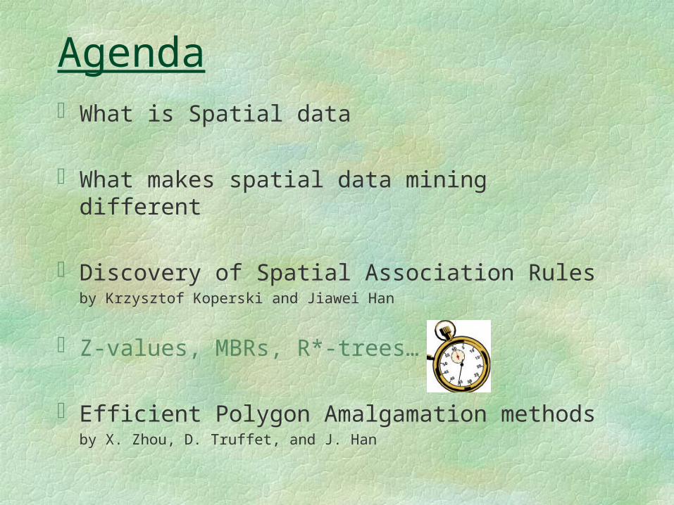
What is Spatial Data?
Objects of types: points lines polygons etc.
Used in/for: GIS - Geographic Information Systems
GPS - Global Positioning System
Environmental studies
etc …
What makes mining Spatial data different? Huge objects
Polygon (3 7.5, 12 -56, 1 2, 3 7.5) Very large object
Heavy computations intersect(Polygon1, line2) contain(Polygon1, Polygon2)
Usually maintain large index tables Z-value Each Spatial object can be indexed by one or
many Z-values
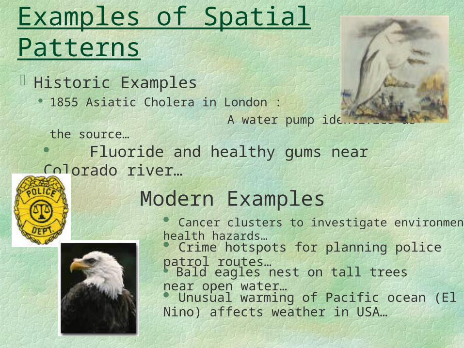
Examples of Spatial Patterns
Historic Examples 1855 Asiatic Cholera in London :
A water pump identified as the source… Fluoride and healthy gums near Colorado river…
Modern Examples Cancer clusters to investigate environment health hazards…
Crime hotspots for planning police patrol routes…
Bald eagles nest on tall trees near open water…
Unusual warming of Pacific ocean (El Nino) affects weather in USA…
Sources:
K. Koperski and J. Han.
[2] Discovery of Spatial Association Rules
In Geographic Information Databases
In Proc. 4th Int'l Symp. on Large Spatial Databases (SSD'95), pp. 47-66, Portland, Maine, Aug. 1995.
X. Zhou, D. Truffet, and J. Han
[3] Efficient Polygon Amalgamation Methods
for Spatial OLAP and Spatial Data Mining
In SSD'99, pp. 167-187, Hong Kong, Aug. 1999.
[1] Discovery of Spatial Association Rules In Geographic Information Databases
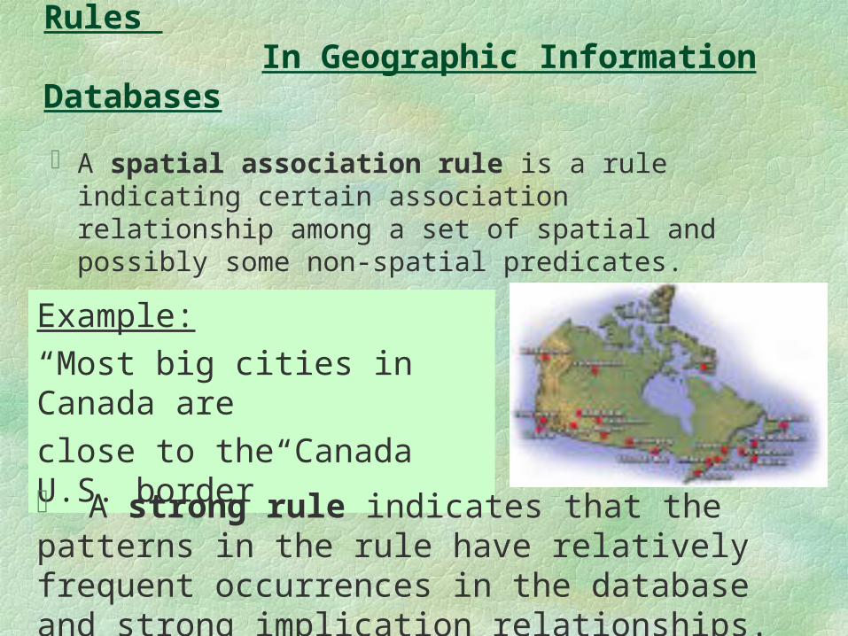
A spatial association rule is a rule indicating certain association relationship among a set of spatial and possibly some non-spatial predicates.
Example:
“Most big cities in Canada are
close to the Canada U.S. border”
A strong rule indicates that the patterns in the rule have relatively frequent occurrences in the database and strong implication relationships.
Discovery of Spatial Association Rules (cont.)More formally,
A spatial association rule is a rule in the form of P 1 … Pm Q 1 … Qn (c%) ,where at least one of the predicates P 1 ,…, Pm , Q 1 ,…, Qn is a spatial predicate, and c% is the confidence of the rule [which indicates that c% of objects satisfying the antecedent of the rule will also satisfy the consequent of the rule].
A set of predicates P is large in set S at level k if the support of P is no less than its minimum support threshold σ`k for level k, and all ancestors of P from the concept hierarchy are large at their corresponding levels.
The confidence of a rule “P Q/S” is high at level k if its confidence is no less than its corresponding minimum confidence threshold φ`k
A rule “P Q/S” is strong if predicate “P Q” is large in set S and the confidence of “P Q/S” is high.
Discovery of Spatial Association Rules (cont.)
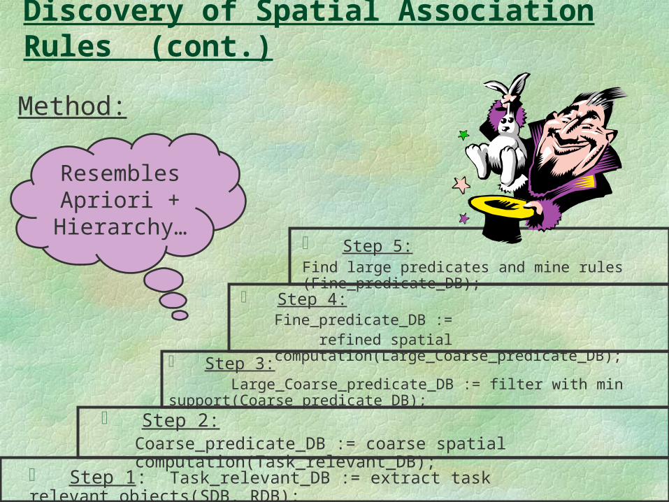
Method:
Step 2: Coarse_predicate_DB := coarse spatial computation(Task_relevant_DB);
Step 3: Large_Coarse_predicate_DB := filter with min support(Coarse predicate DB);
Step 4: Fine_predicate_DB := refined spatial computation(Large_Coarse_predicate_DB);
Step 5: Find large predicates and mine rules (Fine_predicate_DB);
Step 1: Task_relevant_DB := extract task relevant objects(SDB, RDB);
Resembles Apriori +
Hierarchy…
Discovery of Spatial Association Rules (cont.)
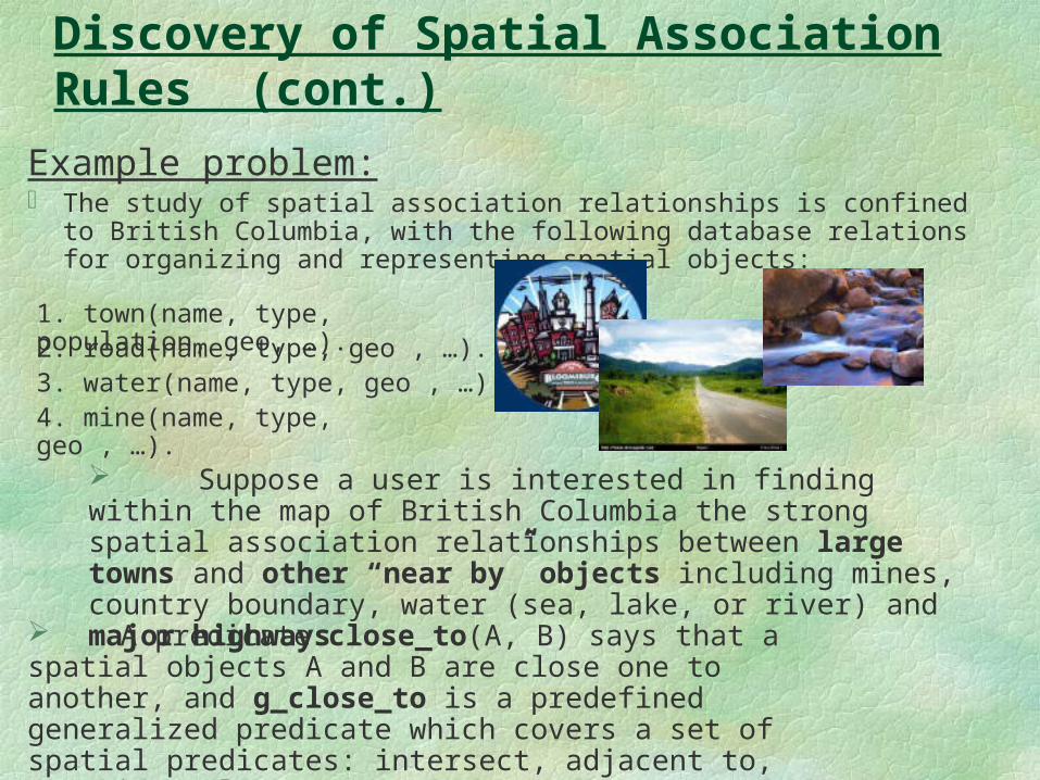
Example problem: The study of spatial association relationships is confined to British Columbia,
with the following database relations for organizing and representing spatial objects:
Suppose a user is interested in finding within the map of British Columbia the strong spatial association relationships between large towns and other “near by” objects including mines, country boundary, water (sea, lake, or river) and major highways
A predicate close_to(A, B) says that a spatial objects A and B are close one to another, and g_close_to is a predefined generalized predicate which covers a set of spatial predicates: intersect, adjacent to, contains, close_to.
1. town(name, type, population, geo, …). 2. road(name, type, geo , …). 3. water(name, type, geo , …). 4. mine(name, type, geo , …).
Discovery of Spatial Association Rules (cont.)
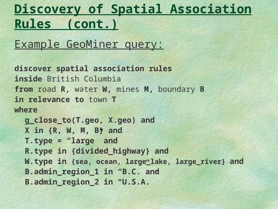
Example GeoMiner query:
discover spatial association rules inside British Columbia from road R, water W, mines M, boundary B in relevance to town T where
g_close_to(T.geo, X.geo) and X in {R, W, M, B} and T.type = “large” and R.type in {divided_highway} and W.type in {sea, ocean, large_lake, large_river} and B.admin_region_1 in “B.C.”and B.admin_region_2 in “U.S.A.”
Discovery of Spatial Association Rules (cont.)
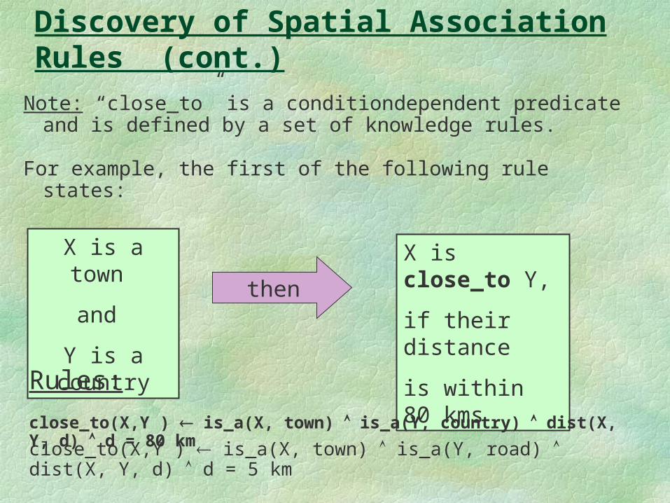
Note: “close_to” is a condition dependent predicate and is defined by a set of knowledge rules.
For example, the first of the following rule states:
X is a town
and
Y is a country
X is close_to Y,
if their distance
is within 80 kms
then
Rules:
close_to(X,Y ) is_a(X, town) is_a(Y, country) dist(X, Y, d) d = 80 km
close_to(X,Y ) is_a(X, town) is_a(Y, road) dist(X, Y, d) d = 5 km
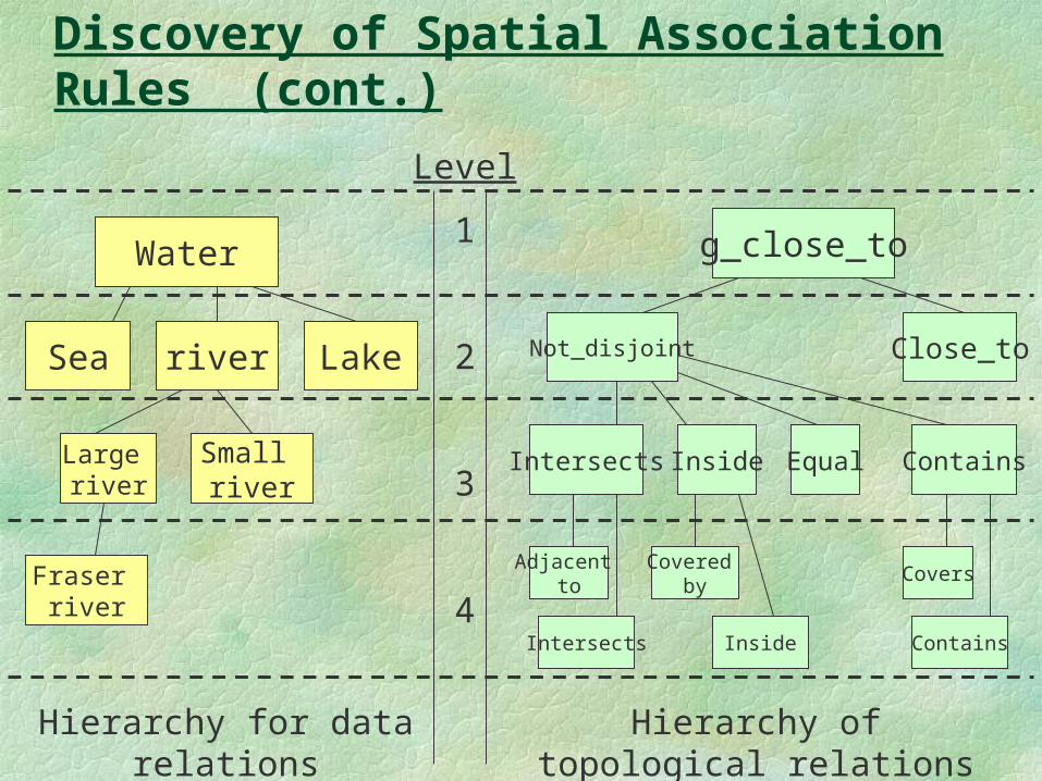
Discovery of Spatial Association Rules (cont.)
Water
riverSea Lake
Large river
Small river
Fraser river
Level
1
2
3
4
g_close_to
Not_disjoint Close_to
Intersects Inside
Adjacent to
Equal Contains
Intersects
Covered by
Inside
Covers
Contains
Hierarchy for data relations Hierarchy of topological relations
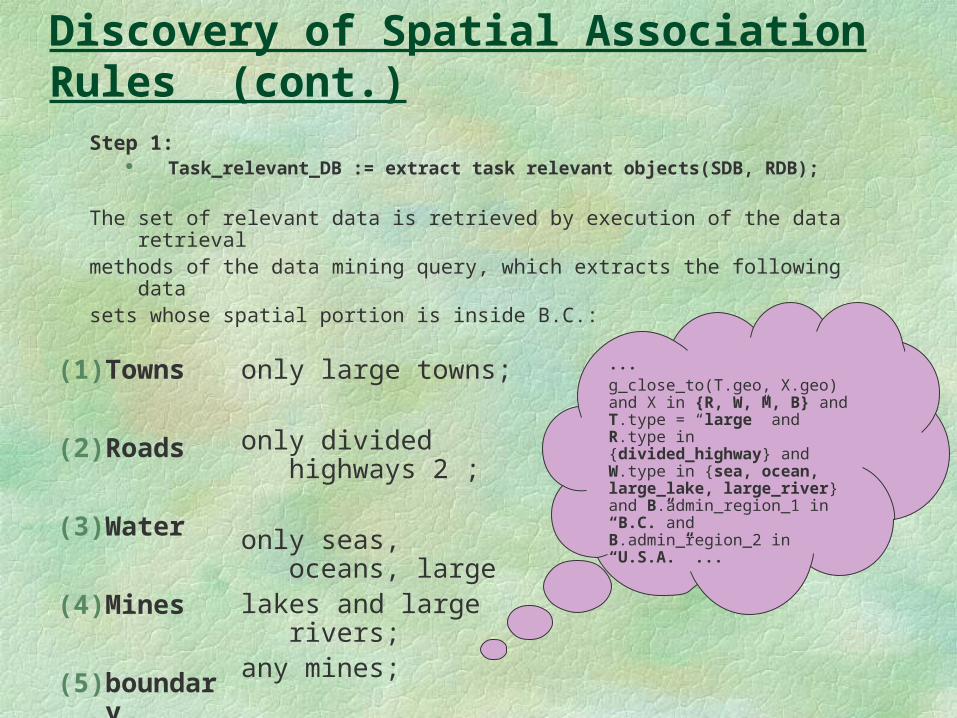
Discovery of Spatial Association Rules (cont.)Step 1:
Task_relevant_DB := extract task relevant objects(SDB, RDB);
The set of relevant data is retrieved by execution of the data retrievalmethods of the data mining query, which extracts the following data sets whose spatial portion is inside B.C.:
... g_close_to(T.geo, X.geo) and X in {R, W, M, B} and T.type = “large” and R.type in {divided_highway} and W.type in {sea, ocean, large_lake, large_river} and B.admin_region_1 in “B.C.”and B.admin_region_2 in “U.S.A.” ...
(1) Towns
(2) Roads
(3) Water
(4) Mines
(5) boundary
only large towns;
only divided highways 2 ;
only seas, oceans, large lakes and large rivers; any mines;
only the boundary of B.C., and U.S.A.
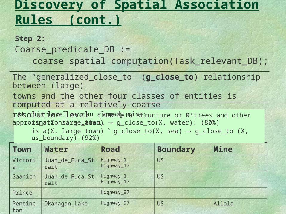
Discovery of Spatial Association Rules (cont.)Step 2:
Coarse_predicate_DB := coarse spatial computation(Task_relevant_DB);
Town Water Road Boundary MineVictoria Juan_de_Fuca_Strait Highway_1, Highway_17 US
Saanich Juan_de_Fuca_Strait Highway_1, Highway_17 US
Prince Highway_97
Pentincton Okanagan_Lake Highway_97 US Allala
… … … … …
At this level we can already mine:is_a(X, large_town) g_close_to(X, water): (80%) is_a(X, large_town) g_close_to(X, sea) g_close_to (X, us_boundary):(92%)
The “generalized_close_to” (g_close_to) relationship between (large) towns and the other four classes of entities is computed at a relatively coarse resolution level. [MBR data structure or R* trees and other approximations] – Later…
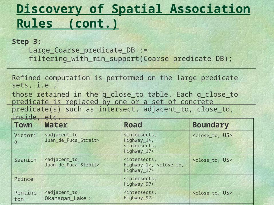
Discovery of Spatial Association Rules (cont.)Step 3:
Large_Coarse_predicate_DB := filtering_with_min_support(Coarse predicate DB);
Town Water Road BoundaryVictoria <adjacent_to, Juan_de_Fuca_Strait> <intersects, Highway_1>,
<intersects, Highway_17><close_to, US>
Saanich <adjacent_to, Juan_de_Fuca_Strait> <intersects, Highway_1>, <close_to, Highway_17>
<close_to, US>
Prince <intersects, Highway_97>
Pentincton <adjacent_to, Okanagan_Lake > <intersects, Highway_97> <close_to, US>
… … … …
Refined computation is performed on the large predicate sets, i.e., those retained in the g_close_to table. Each g_close_to predicate is replaced by one or a set of concrete predicate(s) such as intersect, adjacent_to, close_to, inside, etc.
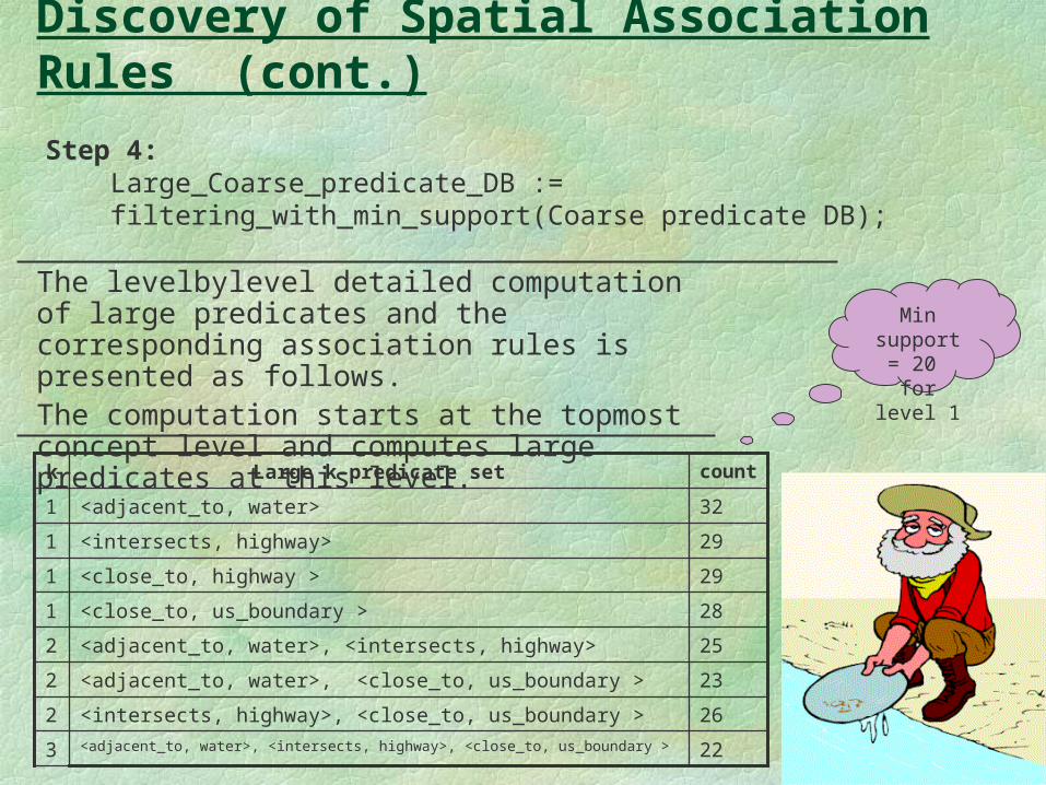
Discovery of Spatial Association Rules (cont.)
Step 4: Large_Coarse_predicate_DB :=
filtering_with_min_support(Coarse predicate DB);
23<adjacent_to, water>, <close_to, us_boundary >2
26<intersects, highway>, <close_to, us_boundary >2
29<intersects, highway>1
29<close_to, highway >1
28<close_to, us_boundary >1
countLarge k-predicate setk
32<adjacent_to, water>1
25<adjacent_to, water>, <intersects, highway>2
22<adjacent_to, water>, <intersects, highway>, <close_to, us_boundary >3
Min support = 20
for level 1
The level by level detailed computation of large predicates and the corresponding association rules is presented as follows. The computation starts at the top most concept level and computes large predicates at this level.
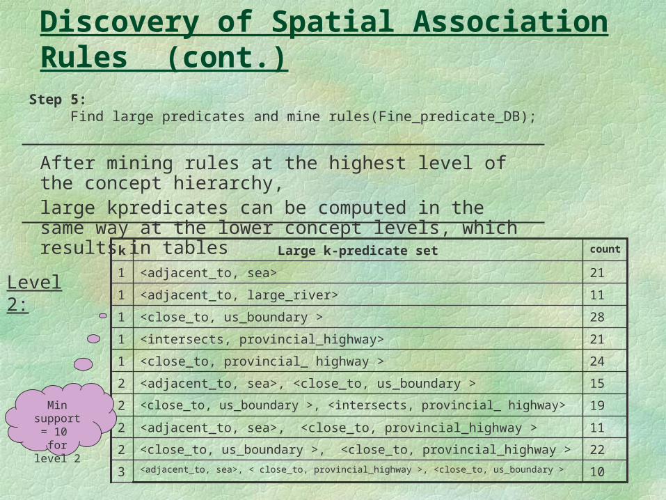
Discovery of Spatial Association Rules (cont.)Step 5:
Find large predicates and mine rules(Fine_predicate_DB);
24<close_to, provincial_ highway >1
11<adjacent_to, large_river>1
11<adjacent_to, sea>, <close_to, provincial_highway >2
22<close_to, us_boundary >, <close_to, provincial_highway >2
28<close_to, us_boundary >1
21<intersects, provincial_highway>1
15<adjacent_to, sea>, <close_to, us_boundary >2
countLarge k-predicate setk
21<adjacent_to, sea>1
19<close_to, us_boundary >, <intersects, provincial_ highway>2
10<adjacent_to, sea>, < close_to, provincial_highway >, <close_to, us_boundary >3
Min support = 10
for level 2
Level 2:
After mining rules at the highest level of the concept hierarchy, large k predicates can be computed in the same way at the lower concept levels, which results in tables
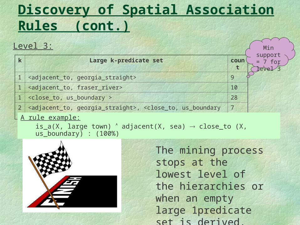
k Large k-predicate set count
1 <adjacent_to, georgia_straight> 9
1 <adjacent_to, fraser_river> 10
1 <close_to, us_boundary > 28
2 <adjacent_to, georgia_straight>, <close_to, us_boundary > 7
Discovery of Spatial Association Rules (cont.)Level 3: Min
support = 7 for level
3
The mining process stops at the lowest level of the hierarchies or when an empty large 1 predicate set is derived.
A rule example:is_a(X, large town) adjacent(X, sea) close_to (X, us_boundary) : (100%)
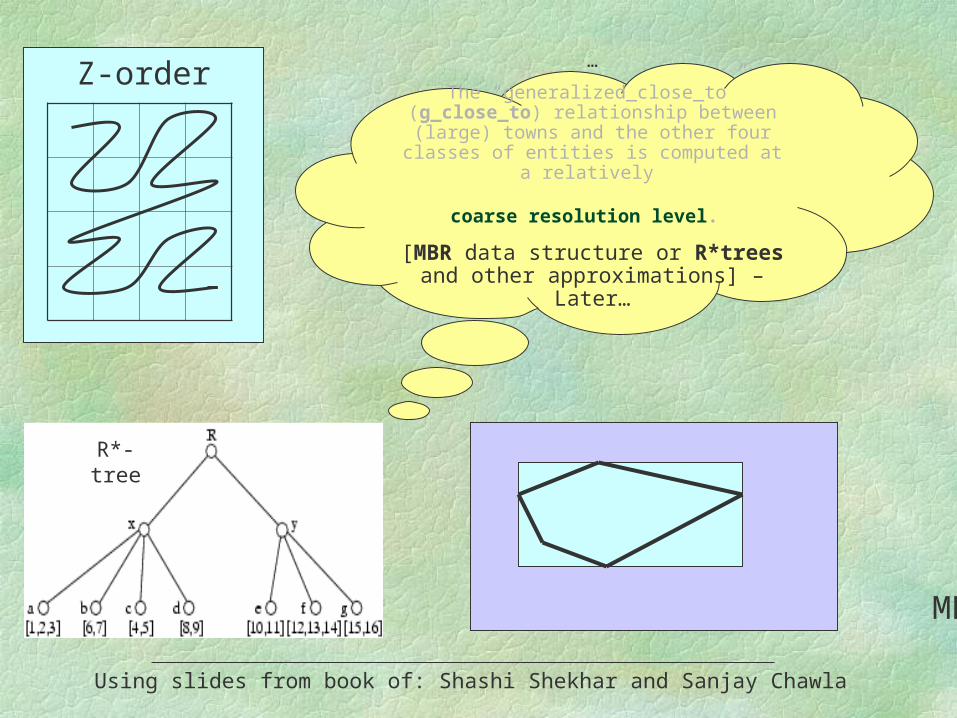
Z-order…
The “generalized_close_to” (g_close_to) relationship between (large) towns and the other
four classes of entities is computed at a relatively
coarse resolution level.
[MBR data structure or R* trees and other approximations] – Later…
Using slides from book of: Shashi Shekhar and Sanjay Chawla
MBR
R*-tree
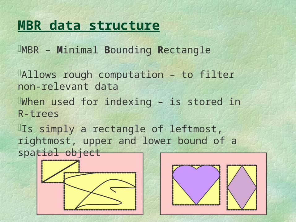
MBR data structure
MBR – Minimal Bounding Rectangle
Allows rough computation – to filter non-relevant data
When used for indexing – is stored in R-trees
Is simply a rectangle of leftmost, rightmost, upper and lower bound of a spatial object
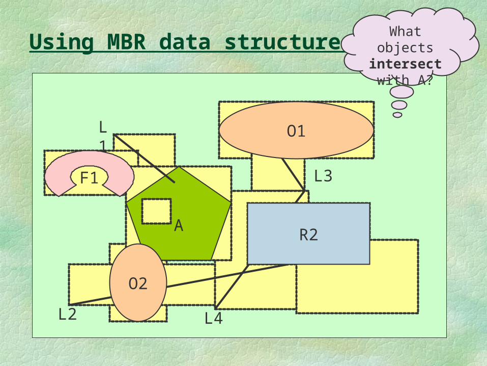
Using MBR data structure
A
R3
O1
O2
R1
L1
L2 L4
L3F1
What objects intersect with
A?
R2
R2
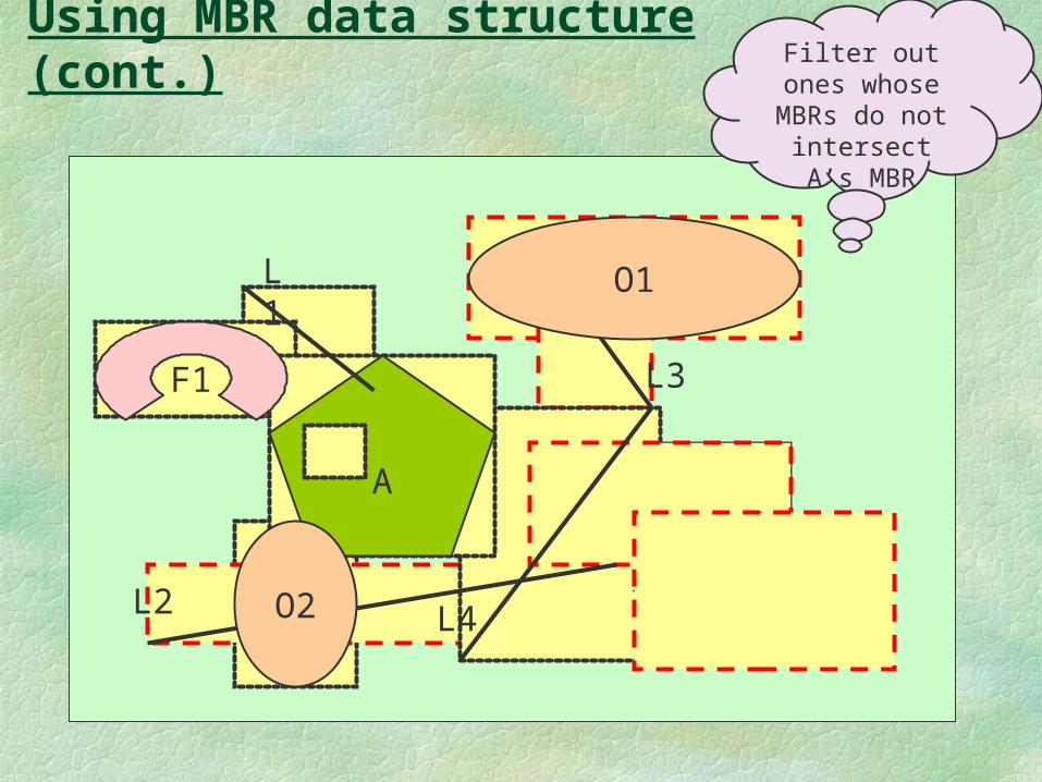
Using MBR data structure (cont.)
A
R3
O1
O2
R1
L1
L2 L4
L3F1
Filter out ones whose MBRs do not intersect A’s
MBR
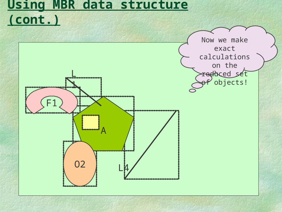
Using MBR data structure (cont.)
A
O2
R1
L1
L4
F1
Now we make exact calculations on the
reduced set of objects!
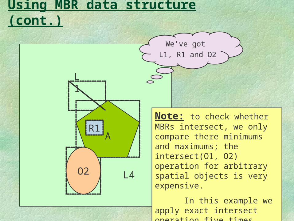
Using MBR data structure (cont.)
A
O2
R1
L1
L4
We’ve got
L1, R1 and O2
Note: to check whether MBRs intersect, we only compare there minimums and maximums; the intersect(O1, O2) operation for arbitrary spatial objects is very expensive.
In this example we apply exact intersect operation five times instead of ten.
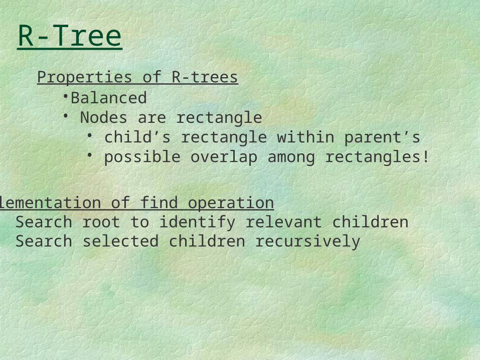
R-TreeProperties of R-trees
•Balanced • Nodes are rectangle
• child’s rectangle within parent’s• possible overlap among rectangles!
Implementation of find operationSearch root to identify relevant childrenSearch selected children recursively
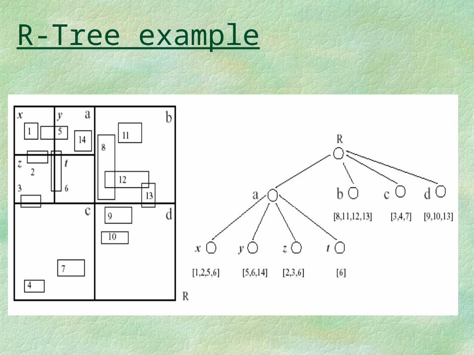
R-Tree example
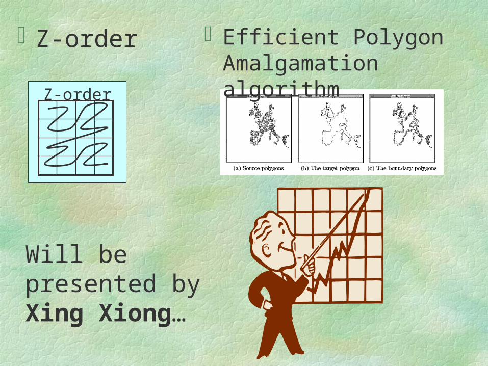
Z-order
Z-order
Will be presented by Xing Xiong…
Efficient Polygon Amalgamation algorithm
Efficient Polygon Amalgamation Methods for Spatial OLAP and Spatial Data Mining
--Xiaofang Zhou, David Truffet, And Jiawei Han
Introduction
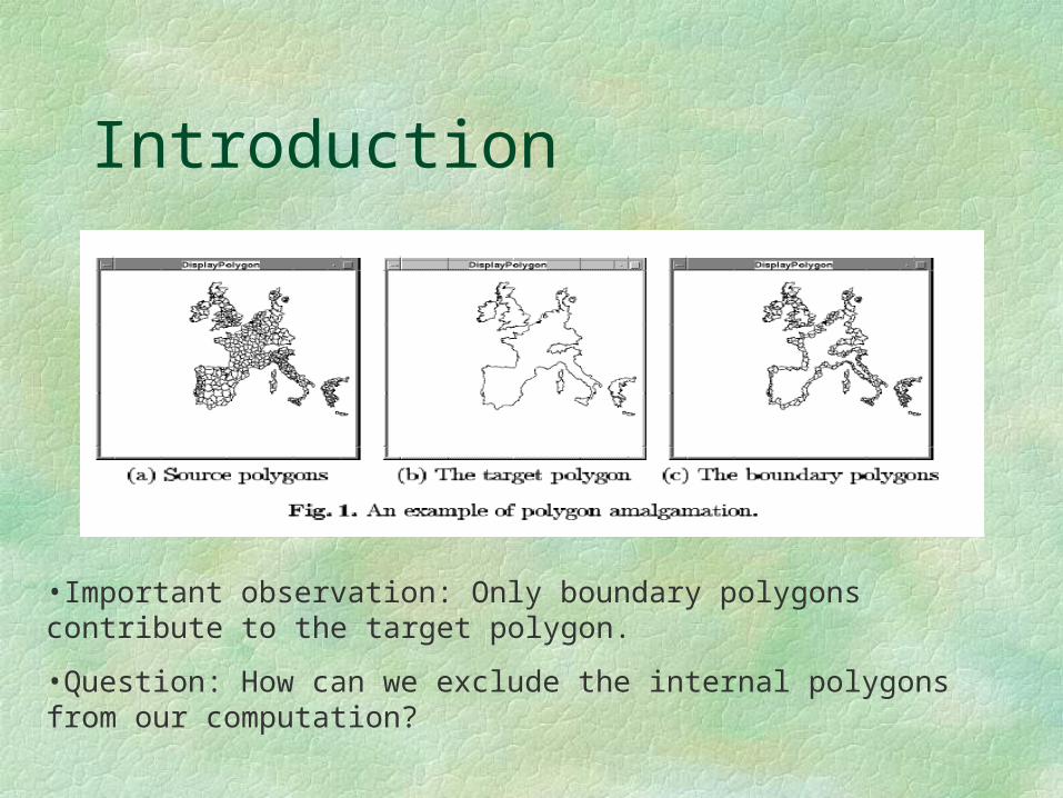
The polygon amalgamation operation computes the boundary of the union of a set of polygons.
This presentation will introduce two efficient polygon amalgamation methods.
Introduction
Why are we interested in amalgamation?It’s a fundamental operation for emerging new applications such as spatial OLAP and spatial data mining.
Example:Roll up operation in OLAP. Group similar spatial objects into clusters in data
mining.
Introduction
•Important observation: Only boundary polygons contribute to the target polygon.
•Question: How can we exclude the internal polygons from our computation?
Introduction
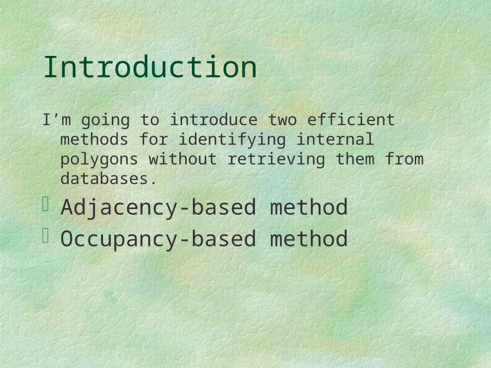
I’m going to introduce two efficient methods for identifying internal polygons without retrieving them from databases.
Adjacency-based methodOccupancy-based method
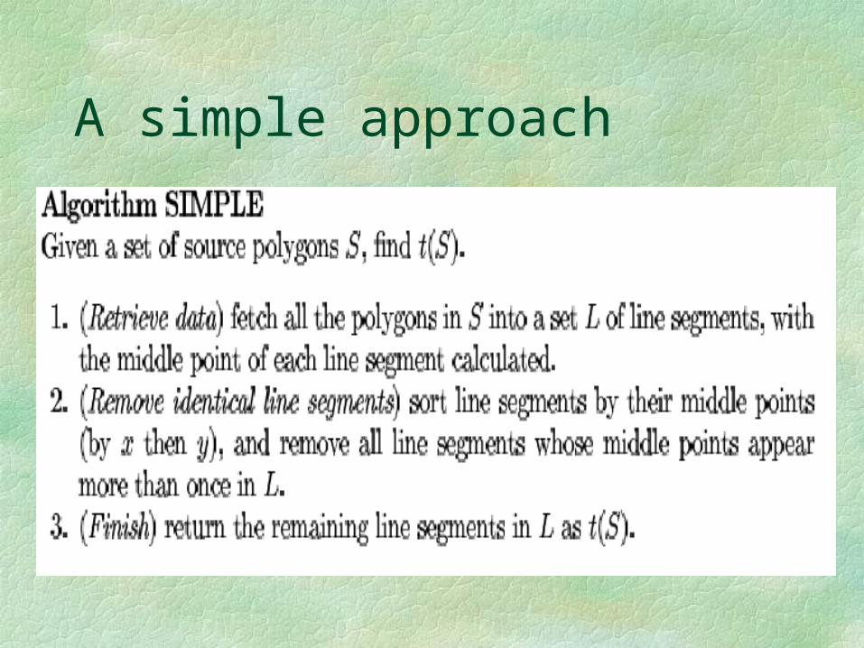
A simple approach
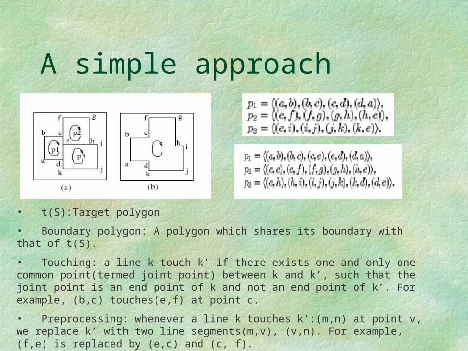
• t(S):Target polygon
• Boundary polygon: A polygon which shares its boundary with that of t(S).
• Touching: a line k touch k’ if there exists one and only one common point(termed joint point) between k and k’, such that the joint point is an end point of k and not an end point of k’. For example, (b,c) touches(e,f) at point c.
• Preprocessing: whenever a line k touches k’:(m,n) at point v, we replace k’ with two line segments(m,v), (v,n). For example, (f,e) is replaced by (e,c) and (c, f).
A simple approach
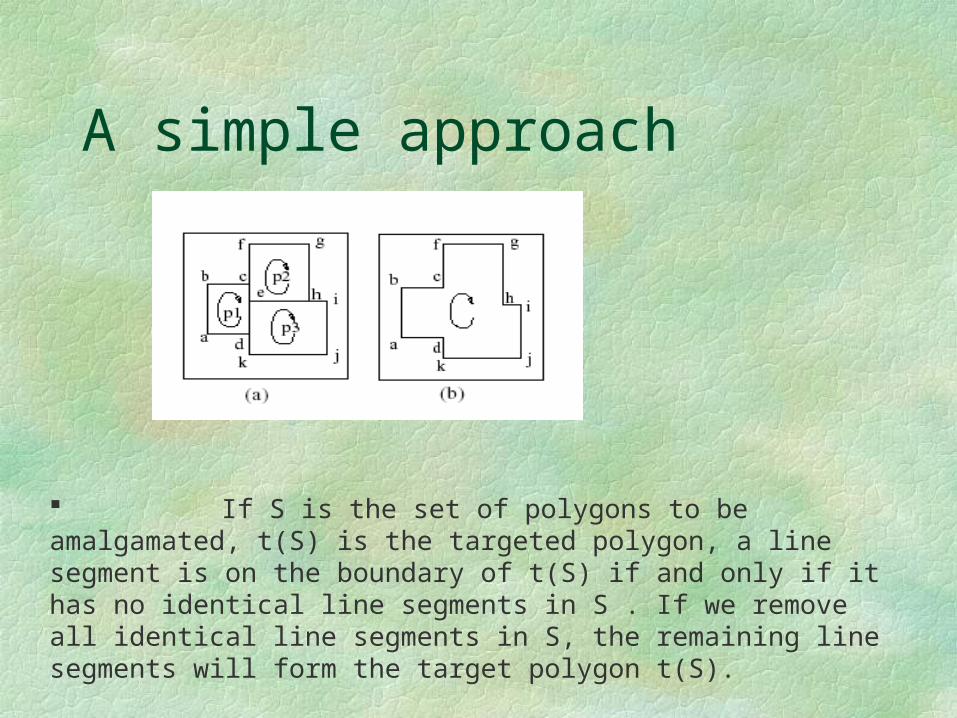
If S is the set of polygons to be amalgamated, t(S) is the targeted polygon, a line segment is on the boundary of t(S) if and only if it has no identical line segments in S . If we remove all identical line segments in S, the remaining line segments will form the target polygon t(S).
A simple approach
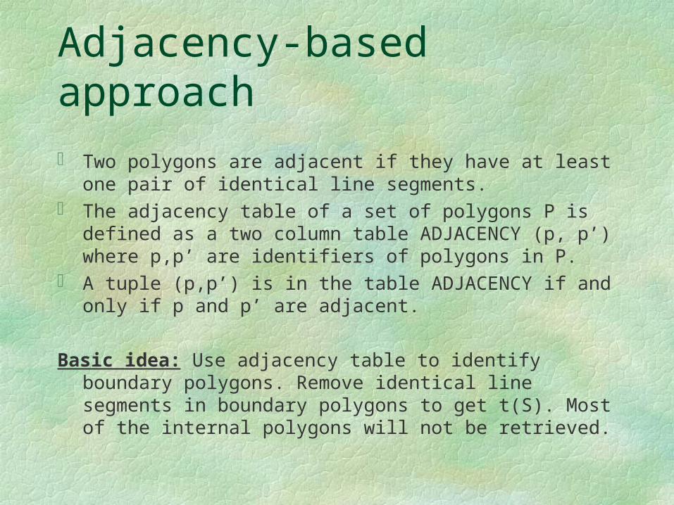
Adjacency-based approach
Two polygons are adjacent if they have at least one pair of identical line segments.
The adjacency table of a set of polygons P is defined as a two column table ADJACENCY (p, p’) where p,p’ are identifiers of polygons in P.
A tuple (p,p’) is in the table ADJACENCY if and only if p and p’ are adjacent.
Basic idea: Use adjacency table to identify boundary polygons. Remove identical line segments in boundary polygons to get t(S). Most of the internal polygons will not be retrieved.
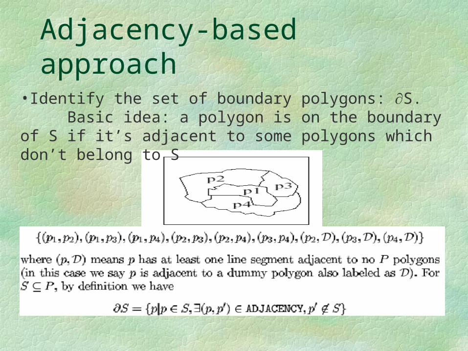
Adjacency-based approach•Identify the set of boundary polygons: S.
Basic idea: a polygon is on the boundary of S if it’s adjacent to some polygons which don’t belong to S
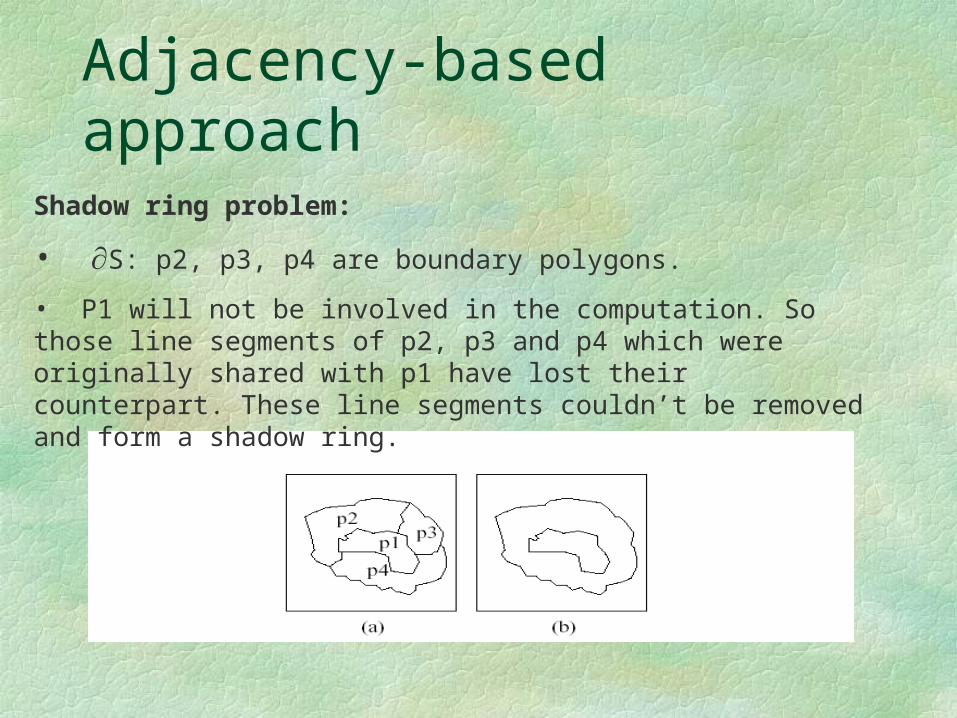
Adjacency-based approachShadow ring problem:
• S: p2, p3, p4 are boundary polygons.
• P1 will not be involved in the computation. So those line segments of p2, p3 and p4 which were originally shared with p1 have lost their counterpart. These line segments couldn’t be removed and form a shadow ring.
Adjacency-based approach
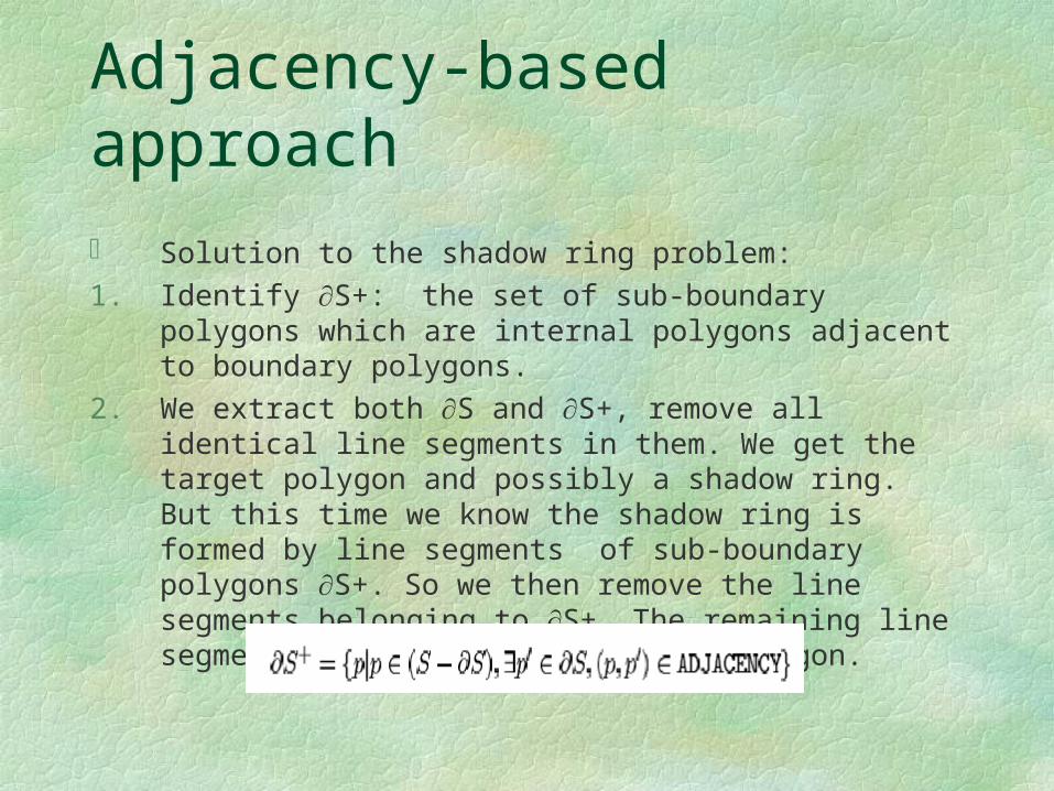
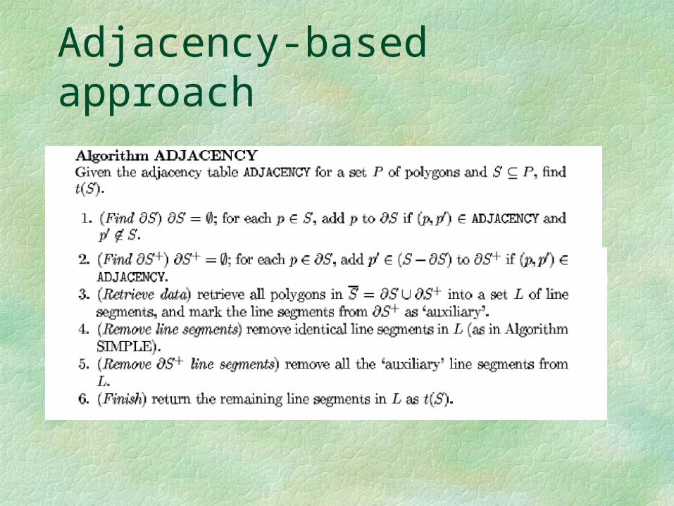
Solution to the shadow ring problem:
1. Identify S+: the set of sub-boundary polygons which are internal polygons adjacent to boundary polygons.
2. We extract both S and S+, remove all identical line segments in them. We get the target polygon and possibly a shadow ring. But this time we know the shadow ring is formed by line segments of sub-boundary polygons S+. So we then remove the line segments belonging to S+. The remaining line segments will form the boundary polygon.
Adjacency-based approach
Occupancy-based approach
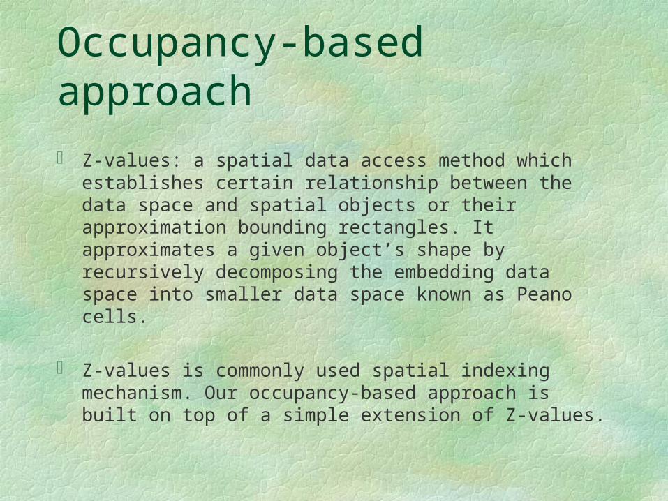
Z-values: a spatial data access method which establishes certain relationship between the data space and spatial objects or their approximation bounding rectangles. It approximates a given object’s shape by recursively decomposing the embedding data space into smaller data space known as Peano cells.
Z-values is commonly used spatial indexing mechanism. Our occupancy-based approach is built on top of a simple extension of Z-values.
Occupancy-based approach
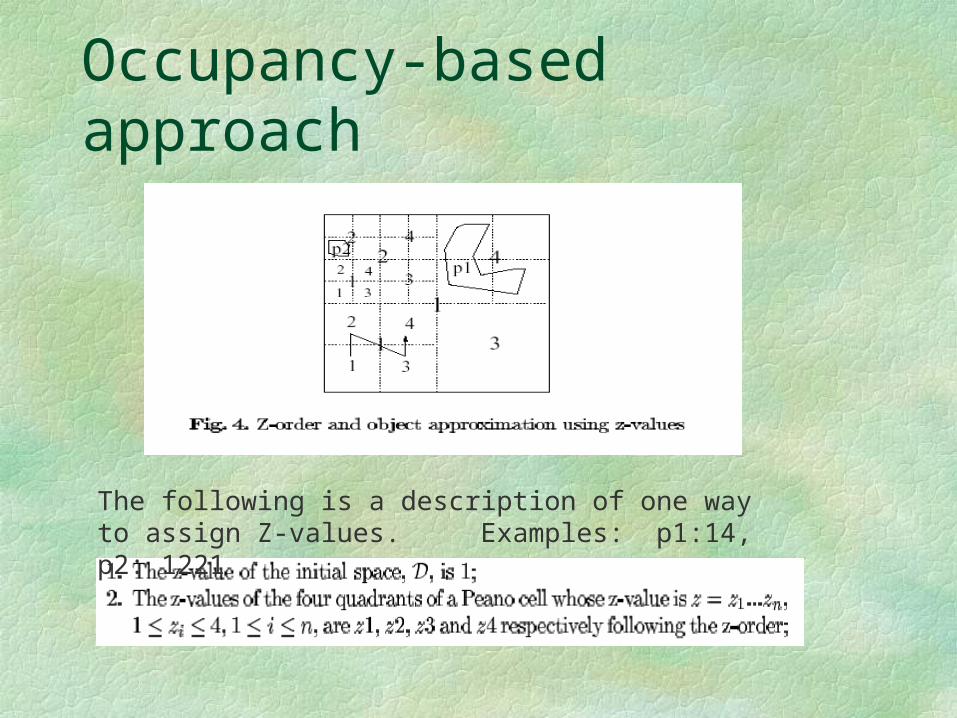
The following is a description of one way to assign Z-values. Examples: p1:14, p2: 1221
Occupancy-based approach
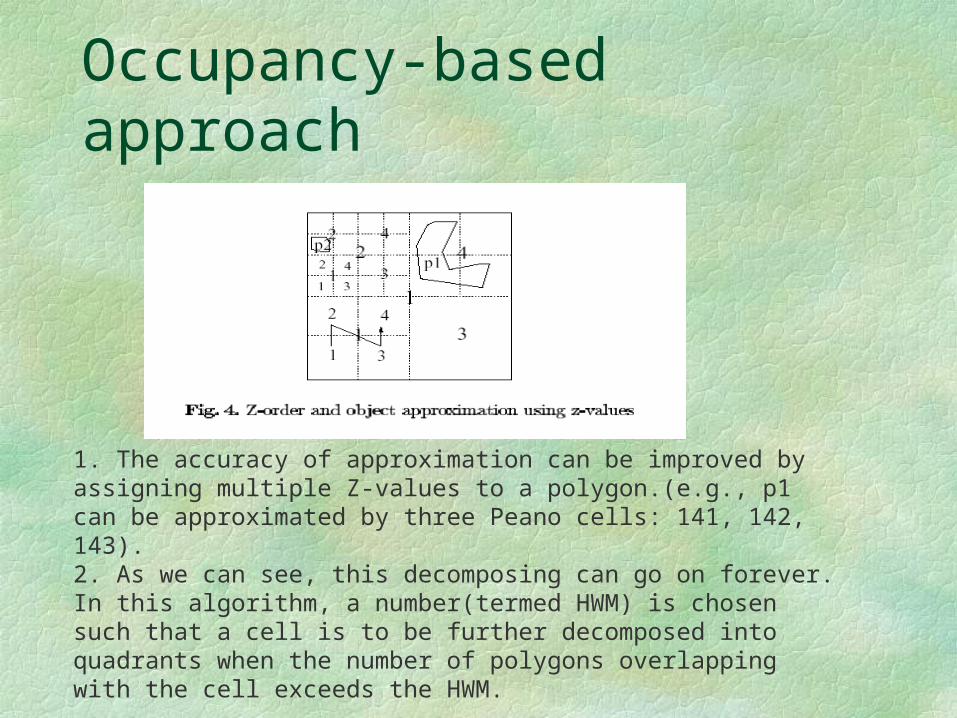
1. The accuracy of approximation can be improved by assigning multiple Z-values to a polygon.(e.g., p1 can be approximated by three Peano cells: 141, 142, 143).2. As we can see, this decomposing can go on forever. In this algorithm, a number(termed HWM) is chosen such that a cell is to be further decomposed into quadrants when the number of polygons overlapping with the cell exceeds the HWM.
Occupancy-based approach
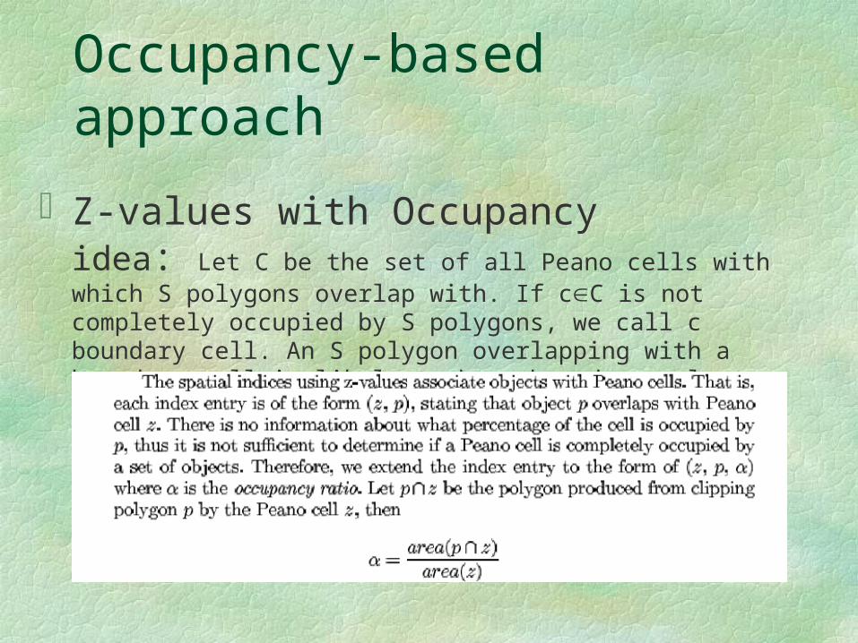
Z-values with Occupancyidea: Let C be the set of all Peano cells with which S polygons overlap with. If cC is not completely occupied by S polygons, we call c boundary cell. An S polygon overlapping with a boundary cell is likely to be a boundary polygon.
Occupancy-based approach
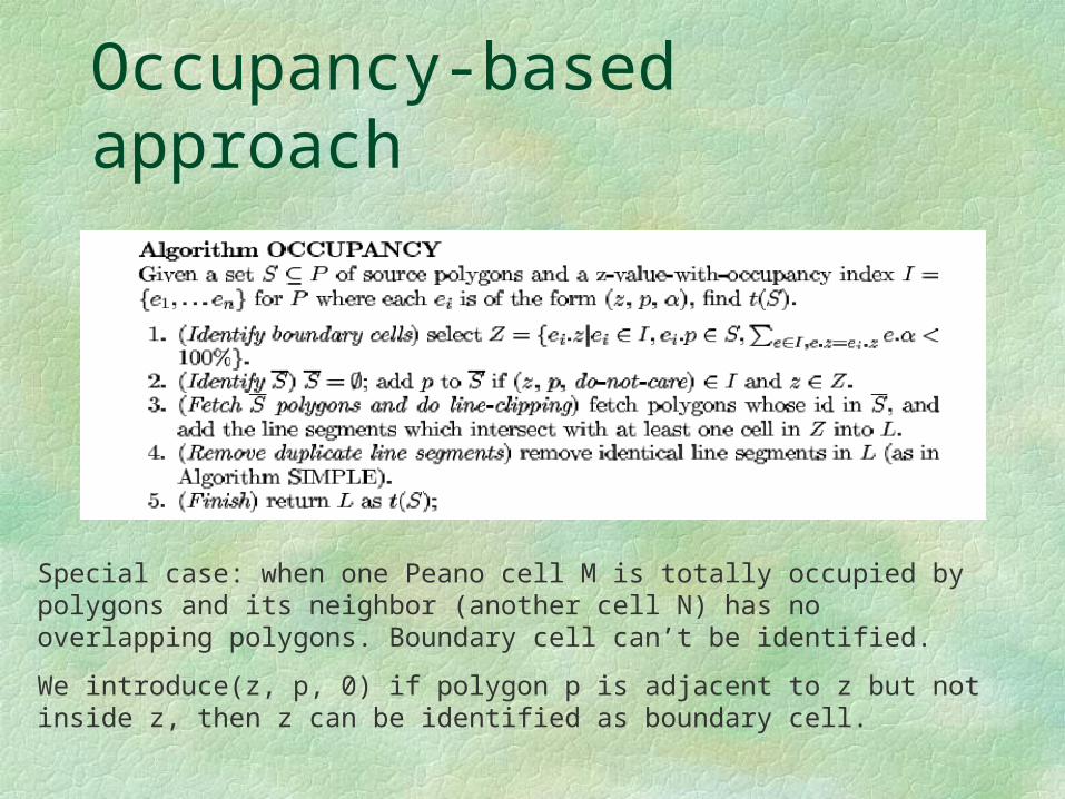
Special case: when one Peano cell M is totally occupied by polygons and its neighbor (another cell N) has no overlapping polygons. Boundary cell can’t be identified.
We introduce(z, p, 0) if polygon p is adjacent to z but not inside z, then z can be identified as boundary cell.
Occupancy-based approach
Two extra points: Occupancy-based approach will not produce shadow rings. Because:1. Any line segment which doesn’t overlap with boundary cells is not part of the
target polygon, and thus can be discarded.
2. Any line segment inside a boundary cell either is part of the target polygon, or its counterpart from another polygon must also be inside this boundary cell.
Fuzzy amalgamation.1. This is a desirable advantage of Occupancy-based method over two other
methods.
2. Instead of defining internal cells as those with 100% occupancy, we can adjust to a low threshold(e.g, 95%). This is useful when user wants to ignore data noises.
Performance
In comparison with SIMPLE algorithm which retrieves all the source polygons, both adjacency-based and occupancy-based algorithm fetch a smaller number of polygons.
SIMPLE algorithm processes all the line segments in the source polygons. Adjacency-based algorithm processes the line segments of the boundary and sub-boundary polygons. Occupancy-based algorithm just processes the line segments which intersects with boundary Peano cells.
Experimental results show that occupancy-based method has achieved a remarkably better overall performance, in particular with an HWM which puts an average of 5-7 polygons to a cell.

And now discussion
© Peter de Sève 1997