Indian Journal of Marine Sciences Vol. 34(2), June 2005, pp. 225-236

ENSO signature in the sea level along the coastline of the Indian subcontinent

K. Srinivas*, P.K. Dinesh Kumar & C. Revichandran National Institute of Oceanography, Regional Centre, P O Box No. 1913, Cochin 682 018, India

*(E-mail: srinivas_kantha@yahoo.co.in ) Received 3 November 2003; revised 9 March 2005

Evidence for the signature of El Nino-Southern Oscillation (ENSO) phenomenon in the monthly mean sea level at 8 tide gauge stations on the west coast and 7 stations on the east coast of the Indian subcontinent is presented. The Southern Oscillation Index (SOI, indicator of the ENSO phenomenon) available continuously from 1933 onwards, was utilized to examine the relationship between sea level and ENSO. The relationship between sea level and SOI is direct, with the sea level decreasing during El Nino years and increasing during La Nina years. The signature of ENSO is particularly conspicuous in the sea level records on the east coast as compared to those on the west coast. Reduced rainfall over the Indian subcontinent and resultant river discharges, remote forcing by interannual zonal winds along the equator and reduced Indonesian Throughflow could be the probable factors explaining the low sea level along the coastline of the Indian subcontinent during ENSO events. The interannual sea level along the coastline of the Indian subcontinent shows more or less synchronous movement-the rise and fall is nearly simultaneous. At low frequency, spatial coherence of sea level is very large.

[Key words: Sea level, El Nino-Southern Oscillation, Southern Oscillation Index, Indian coastline]

Introduction Monthly mean sea level can be used to monitor the large scale, low frequency circulation of the oceans1-4

and can also be used for predicting the seasonal rainfall5, a very important meteorological parameter for agriculture related activities. A major component of the climate of the Indian subcontinent is the summer monsoon, which is linked to global climate through planetary scale processes in the atmosphere and ocean. Shankar & Shetye6 showed that interdecadal sea level changes along the Indian coast and the variability of the monsoon rainfall are inter-connected. Das & Radhakrishna7 analysed the sea level records at Bombay, Cochin, Madras and Visakhapatnam, concluding that all the stations show both long period (50-60 year period), and shorter period fluctuations of 4.5 to 5.7 years. Perigaud & Delecluse8 have discussed Indian Ocean sea level variability using Geosat altimeter data of 4.5 years duration. They showed the signature of Rossby waves west of the Indo-Pacific throughflow region, in the southern tropical Indian Ocean. Clarke & Liu9 demonstrated that the atmospheric pressure corrected sea level is correlated along the northern Indian Ocean boundary. Murtugudde & Busalacchi10 examined the sea level records at some stations along the Indian coastline, in their study on the interannual variability of the dynamics and thermodynamics of

the tropical Indian Ocean, and the results are similar to Clarke & Liu9 with regard to the sea level variability. Shankar and Shetye11 showed that the mean sea level along the coast of India is higher in the Bay of Bengal than in the Arabian Sea, the difference in sea level between Visakhapatnam and Bombay being about 30 cm. Based on simulations from a one-and-half layer reduced gravity model, they attributed this difference to the mean, large-scale wind forced circulation (~60%) and the alongshore gradient in salinity (~40%). The largest non-tidal changes of sea level evident in the Pacific Ocean are due to ENSO events. During these ENSO events, approximately one metre of water column is transferred from the western equatorial Pacific to the South American coast, with changes clearly noticeable in tide gauge records4,12,13 and in satellite altimetry14. Several compilations on the subject of sea level and its relationship with ENSO are available in the literature2,3,9,12,15-21. The probable influence of ENSO events on the coastal sea level along the Indian subcontinent has not been reported in the literature. The main objective of the present study is to examine the relationship between Southern Oscillation Index (SOI) and the corresponding sea level records at different tide gauge stations along the coastline of the Indian subcontinent.

INDIAN J. MAR. SCI., VOL. 34, No. 2, JUNE 2005

226

Materials and Methods Tide gauge data on sea level collected at eight stations along the west coast of India (eastern Arabian Sea) viz. Cochin, Mangalore, Karwar, Mormugao, Bombay, Bhavnagar, Kandla, and Karachi (Pakistan) and seven stations along the east coast of India (western Bay of Bengal) viz. Tuticorin, Thangacchimadam, Nagapatnam, Madras, Visakhapatnam, Paradip and Sagar Island were utilized in this study (Fig. 1 and Table 1). For the west coast, a total of 276 station years of data were used, whereas for the east coast it was 214. Island stations far off from the main coastline were not considered in this study. Karachi is included in the present study, as it is situated just outside the Tropic of Cancer and is also the northernmost limit of the eastern Arabian Sea. The latitudinal distance between the extreme stations on the west coast (Cochin and Karachi) is 1650 km while on the east coast (Tuticorin and Sagar Island) it is 1430 km. The data used (Table 1) in this study were provided by the Permanent Service for Mean Sea Level (PSMSL), UK, which compiles and archives monthly and annual mean sea level data received from different national organisations throughout the world22. The Revised Local Reference (RLR) data of the PSMSL that are more accurate than the other data sets (e.g. metric data sets, also published by PSMSL)-were used in this analysis. The monthly mean values were computed by averaging hourly values of a tidal record for each month.

The dynamically relevant subsurface pressure near the water surface is the sum of pressure due to the measured sea level and the fluctuating atmospheric pressure. In an earlier study, Clarke & Liu9 showed that the amplitude of atmospheric pressure is only about 25% of that of sea level at Bombay, Mangalore, Madras and Visakhapatnam and that there is very little variation along the boundary. Since the atmospheric pressure record at Bombay is the longest, they used it to adjust the pressure at all the sea level stations. In the present study also this adjustment for atmospheric pressure was done using Bombay mean sea level atmospheric pressure data, published by Parthasarathy et al23. However, in a more recent study, the monthly mean sea level pressure series in a tabulated form, dating way back from 1796 at Madras is available24. The detrended anomaly of atmospheric pressure has an amplitude of about 18% of that of the detrended anomaly of observed sea level at Bombay (based on the ratio of the standard deviations). The sea level (cm) was corrected by adding the equivalent of atmospheric pressure in centimeters of water. This was done prior to any statistical processing (separation of anomalous components, trends, smoothening, etc.). In the following discussion, sea level will refer to the pressure-corrected sea level unless otherwise explicitly mentioned.

Fig. 1—Station location map

Table 1—Details of the sea level data used in the present study

Station 1 2 3

West coast

Karachi 1937 1947 11 Kandla 1950 1987 38 Bhavnagar 1937 1955 19 Bombay 1878 1988 111 Mormugao 1969 1980 12 Karwar 1970 1988 19 Mangalore 1961 1976 16 Cochin 1939 1988 50

Total - - 276

East coast

Tuticorin 1964 1980 17 Thangacchimadam 1969 1983 15 Nagapatnam 1971 1988 18 Madras 1952 1988 37 Visakhapatnam 1937 1988 52 Paradip 1966 1988 23 Sagar Island 1937 1988 52

Total - - 214

1—Starting year of data 2—Ending year of data 3—Total number of years

SRINIVAS et al.: ENSO SIGNATURE IN THE SEA LEVEL

227

The SOI [Southern Oscillation Index] series is the standardized pressure difference between Tahiti and Darwin25. The extreme values of SOI have received attention because of the association of strong negative values with occurrence of El Nino (warm) events and strong positive values with La Nina (cold) events. Continuous monthly time series data on SOI were available only from 1933 onwards, and the data prior to this year were discontinuous, with large gaps. For the 1933-1988 period, the highest positive value of 2.9 (La Nina) occurred during November, 1973 and the highest negative value of 4.6 (El Nino) occurred during February, 1983. Anomalies of the monthly mean sea level at various stations were determined by removing the mean seasonal cycle and then the series were detrended. These data were then smoothened with a 13-month moving average for the estimation of the correlation coefficients and associated statistical parameters (percentage variance accounted by the linear regression, slope, and standard error on slope of the regression line), with detrended and 13-month moving averages of SOI. The data were detrended to remove the secular trends. Smoothening with a 13-month moving average (functions as a low pass filter) involves the loss of 6 data points each at both ends of the data record i.e. a total of 12 data points, but it helps in removing irregular fluctuations. Only these smoothened data are discussed in the text.

The correlation coefficients between the detrended 13-month smoothened anomalies of sea level at each station against the other fourteen stations were also calculated. This was done to examine the spatial coherence of sea level along the Indian subcontinent. To determine whether there is any serial correlation in the time series26-27, Durbin-Watson “D” test was performed. The “D” statistic was less than 0.10 for all the stations, suggesting highly significant serial correlation in the data. Results and Discussion Statistics of the observed sea level and atmospheric pressure time series Much of the material presented in this section is from a study conducted with the same data, although in a different context28. However, the data in the present study pertain to pressure corrected sea level whereas the data used in the referred study were observed sea level. The standard deviation of the observed data and anomalies (de-seasonalised data) were generally found to be high along the east coast, as compared to the west coast, suggesting very energetic, seasonal as well as interannual signals along the east coast29,30 (Table 2). The monthly anomalies were determined by subtracting the mean

Table 2—Statistics of the sea level (cm) time series at various stations along the west and east coasts of the Indian subcontinent as well as that for the atmospheric pressure (mb) series at Bombay.

1 2 3 4 5 6 7 West coast

Karachi 6.0 11.6 3.4 4.9 32.8 27.0 58.7 Kandla 12.0 17.6 5.0 10.9 17.5 85.3 8.2 Bhavnagar 26.8 63.2 22.1 15.1 68.2 98.3 1.0 Bombay 6.7 11.8 3.4 5.8 26.1 23.0 47.4 Mormugao 7.4 18.1 6.2 4.0 70.5 91.4 3.3 Karwar 9.0 21.4 6.9 5.8 58.2 82.4 13.6 Mangalore 8.5 23.4 5.9 6.1 49.2 1.8 41.6 Cochin 8.1 18.4 6.0 5.4 55.3 84.0 8.1 Bombay – pressure 3.7 10.3 3.5 1.0 93.1 97.2 1.8

East coast Tuticorin 7.5 13.0 4.6 5.9 37.6 75.2 22.6 Thangacchimadam 17.5 47.1 15.5 8.1 78.3 83.4 12.5 Nagapatnam 13.3 38.5 12.0 5.7 81.5 55.3 40.4 Madras 11.1 30.2 8.9 6.6 64.2 46.2 48.8 Visakhapatnam 15.6 43.6 14.0 6.9 80.3 75.8 21.3 Paradip 16.9 40.7 15.2 7.4 81.1 91.5 7.0 Sagar Island 21.9 48.3 18.1 12.3 68.2 96.1 3.3

1—Standard deviation of the entire time series 2—Range of the mean seasonal cycle 3—Standard deviation of the mean seasonal cycle 4—Standard deviation of the anomaly time series 5—Seasonal variance (%) contained in the entire series given by:- 100*(1-Varres/Varobs), where Varres is the variance of

the residual time series (i.e. anomalies) and Varobs is the variance of the original time series 6—Contribution of the annual component to the total variance of the mean seasonal cycle (%) 7—Contribution of the semi-annual component to the total variance of the mean seasonal cycle (%)

INDIAN J. MAR. SCI., VOL. 34, No. 2, JUNE 2005

228

monthly sea level for each month from the corresponding month of the entire time series. Bhavnagar on the west coast appears to have the highest seasonal and interannual variations, probably due to the discharge of the Narmada and other rivers, as well as due to its unique location. The seasonal sea level variances (%) contained in the entire time series for the various stations show higher values at stations on the east coast than those on the west coast. The seasonal cycle is strong along the east coast as compared to the west coast, in terms of year-to-year variability. At least six stations (out of seven) have a value of more than 64%, along the east coast, whereas along the west coast only two (out of eight) have a value more than 64%. Along the west coast, the variance was maximum at Mormugao (70.5%) and minimum at Kandla (17.5%) whereas along the east coast, the variance was maximum at Nagapatnam (81.5%) and minimum at Tuticorin (37.6%). The seasonal cycle is complex and shows remarkable variability, even at closely spaced stations. This complexity seems to be more conspicuous along the west coast than on the east coast. In earlier studies on seasonal variability of sea level along the coastline of the Indian subcontinent, a few stations showed highly significant relationship with coastal alongshore current30. Reversals in the currents were clearly reflected in the sea level changes, thus suggesting that the sea level records at these stations would be useful for long term monitoring of the surface geostrophic flow along the coastline of India. The relationship between observed sea level and coastal alongshore current is due mainly to the Coriolis force, which is responsible for deflecting the mass. Due to the action of the Coriolis force, a slope is created perpendicular to the direction of the currents and hence a change in sea level along the coast accompanies the change in coastal currents. When looking in the direction of the flow in the northern hemisphere, the height of the sea level is greater on the right hand side and lower on the left hand side.

The seasonal variance of the coastal alongshore currents was found to be more off the east coast than off the west coast of India, indicating that the alongshore currents are more energetic along the east coast as compared to the west coast30. The western boundary currents are characteristically fast, deep and narrow while the eastern boundary currents are characteristically slow, shallow and wide. Currents driven by the alongshore density difference could be stronger along the east coast than off the west coast,

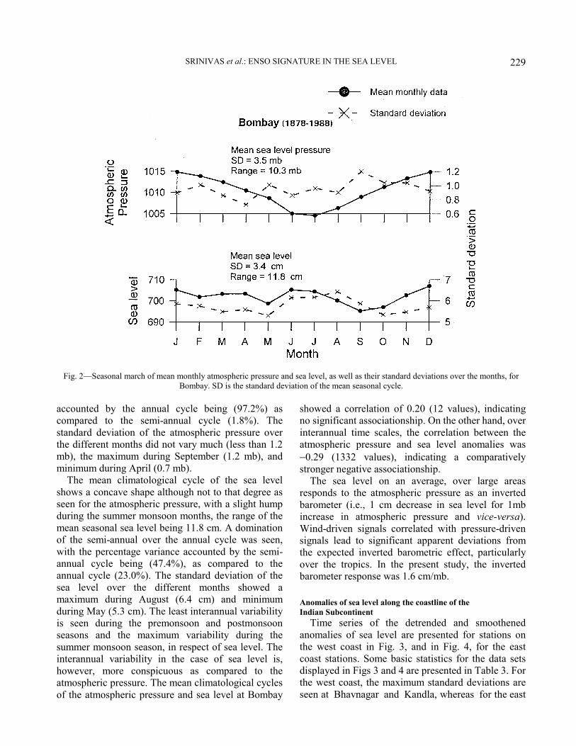
because of the substantial river discharge into the Bay of Bengal, which is more than four times that into the Arabian Sea. The stronger coastal currents could be the reason for higher ranges in sea level along the east coast. The interannual variability in sea level also shows a complex nature along the west coast, whereas along the east coast, the maximum interannual variability was consistently seen during November, probably due to the interannual variation in the rainfall over the Indian subcontinent and associated river discharge, during that month. The annual maximum in rainfall was also seen during that month for some of the stations30. The percentage variances explained by the annual, semi-annual and ter-annual components of the climatological mean seasonal cycle of the sea level and atmospheric pressure, which were determined by harmonic analysis, are presented in Table 2. These are presented to appreciate the dominance of the particular component (annual or semi-annual). A domination of the annual over the semi-annual cycle was seen at five out of eight stations along the west coast, whereas it was six out of seven stations, along the east coast. Further, out of the fifteen stations, a strong domination of the annual over the semi-annual cycle was seen at ten stations. In general, the annual component dominated the semi-annual component, for all the stations, except for Karachi, Bombay, Mangalore and Madras. At Mangalore, the ter-annual component28 was the most dominant one (44.8%), while the contribution by the annual component was hardly 2%. Bombay also showed a relatively high value of about 20% for the ter-annual component28. The ter-annual component was less than 4%, for all the east coast stations28. The seasonal variance (%) contained in the entire time series for the atmospheric pressure suggested very good seasonality (93.1). In other words, the seasonal cycle repeats itself year to year, in a more or less similar manner. It is the only series having strong seasonality among the ones presented in Table 2. To appreciate better the relationship between the seasonal and interannual variations of atmospheric pressure and sea level at Bombay, the march of the mean monthly data on the two parameters, as well as that of the standard deviations over a particular month, for the entire period of study are presented (Fig. 2). The mean climatological cycle of the atmospheric pressure shows a concave shape, the range being 10.3 mb. A very strong domination of the annual over the semi-annual cycle was seen, with the percentage variance

SRINIVAS et al.: ENSO SIGNATURE IN THE SEA LEVEL

229

accounted by the annual cycle being (97.2%) as compared to the semi-annual cycle (1.8%). The standard deviation of the atmospheric pressure over the different months did not vary much (less than 1.2 mb), the maximum during September (1.2 mb), and minimum during April (0.7 mb). The mean climatological cycle of the sea level shows a concave shape although not to that degree as seen for the atmospheric pressure, with a slight hump during the summer monsoon months, the range of the mean seasonal sea level being 11.8 cm. A domination of the semi-annual over the annual cycle was seen, with the percentage variance accounted by the semi-annual cycle being (47.4%), as compared to the annual cycle (23.0%). The standard deviation of the sea level over the different months showed a maximum during August (6.4 cm) and minimum during May (5.3 cm). The least interannual variability is seen during the premonsoon and postmonsoon seasons and the maximum variability during the summer monsoon season, in respect of sea level. The interannual variability in the case of sea level is, however, more conspicuous as compared to the atmospheric pressure. The mean climatological cycles of the atmospheric pressure and sea level at Bombay

showed a correlation of 0.20 (12 values), indicating no significant associationship. On the other hand, over interannual time scales, the correlation between the atmospheric pressure and sea level anomalies was −0.29 (1332 values), indicating a comparatively stronger negative associationship. The sea level on an average, over large areas responds to the atmospheric pressure as an inverted barometer (i.e., 1 cm decrease in sea level for 1mb increase in atmospheric pressure and vice-versa). Wind-driven signals correlated with pressure-driven signals lead to significant apparent deviations from the expected inverted barometric effect, particularly over the tropics. In the present study, the inverted barometer response was 1.6 cm/mb. Anomalies of sea level along the coastline of the Indian Subcontinent Time series of the detrended and smoothened anomalies of sea level are presented for stations on the west coast in Fig. 3, and in Fig. 4, for the east coast stations. Some basic statistics for the data sets displayed in Figs 3 and 4 are presented in Table 3. For the west coast, the maximum standard deviations are seen at Bhavnagar and Kandla, whereas for the east

Fig. 2—Seasonal march of mean monthly atmospheric pressure and sea level, as well as their standard deviations over the months, for Bombay. SD is the standard deviation of the mean seasonal cycle.

INDIAN J. MAR. SCI., VOL. 34, No. 2, JUNE 2005

230

Fig. 3—Detrended and 13-month moving averaged monthly mean sea level anomalies at different stations along the west coast of the Indian subcontinent. The y-axes scales are different. The bottom panel contains the detrended and 13-month moving averages of the SOI

Fig. 4—Detrended and 13-month moving averaged monthly mean sea level anomalies at different stations along the east coast of the Indian subcontinent. The y-axes scales are different. The bottom panel contains the detrended and 13-month moving averages of the SOI

SRINIVAS et al.: ENSO SIGNATURE IN THE SEA LEVEL

231

coast, it is at Sagar Island. The stations that showed an anomaly range over 25 cm, include Sagar Island, followed by Kandla and Bhavnagar. It is possible that the large range in anomalies seen for Sagar Island Table 3—Statistics of the smoothened anomalies of sea level (cm) Station Standard

deviation Minimum value of anomaly

Maximum value of anomaly

Range of anomaly

West coast Karachi 2.1 -7.2 2.9 10.1 Kandla 6.0 -12.7 14.3 27.0 Bhavnagar 6.6 -12.4 14.0 26.4 Bombay 2.4 -6.1 6.4 12.5 Mormugao 1.4 -3.1 2.5 5.6 Karwar 2.5 -7.2 6.4 13.6 Mangalore 2.2 -3.9 5.3 9.2 Cochin 3.3 -8.0 8.6 16.6

East coast

Tuticorin 3.9 -5.6 13.2 18.8 Thangacchimadam 3.3 -5.8 6.3 12.1 Nagapatnam 2.5 -4.8 6.6 11.4 Madras 3.1 -8.5 6.3 14.8 Visakhapatnam 3.3 -7.9 7.4 15.3 Paradip 3.7 -8.6 8.3 16.9 Sagar Island 8.7 -21.8 16.7 38.5

and Bhavnagar could be the result of freshwater discharge of rivers. The bottom curves in both the figures show the detrended and smoothened SOI. The drop in sea level associated with the drop in SOI is clearly seen at most of the stations. The drop associated with the events in the El Nino years of 1972-73, 1982-83 and 1987-88 are clearly brought out for both the coasts. This phenomenon is particularly conspicuous along the east coast. Table 4 shows the correlation coefficients (at zero lag) between the SOI and the sea level anomalies, together with the slopes of the corresponding regression lines and the percentage of variation explained by the correlation coefficients for individual stations. There was, however, no significant difference in correlation between the observed sea level (uncorrected for the effect of atmospheric pressure) and SOI/pressure corrected sea level and SOI. This suggests that the effect of atmospheric pressure variation on sea level at interannual time scales may not be that important along the coastline of the Indian subcontinent. Generally, a significant correlation exists between the anomalies of sea level and SOI (Table 4). With the exception of two stations on the west coast

Table 4—Correlation between the SOI and sea level anomalies at stations along the Indian subcontinent, for the data presented in Figures 3 and 4.

Station 1 2 3 4 5 6

West coast

Karachi 120 -0.265** 0.187 0.244 7.00 -0.752±0.66 Kandla 444 0.179** 0.096 0.125 3.19 1.556±1.06 Bhavnagar 216 0.110ns 0.136 0.178 1.21 - Bombay 660 0.188** 0.081 0.106 3.52 0.681±0.36 Mormugao 132 -0.124ns 0.173 0.226 1.54 - Karwar 216 0.461** 0.149 0.194 21.26 1.526±0.52 Mangalore 180 0.570** 0.169 0.221 32.51 1.984±0.56 Cochin 588 0.372** 0.088 0.114 13.82 1.735±0.46

East coast Tuticorin 192 0.191** 0.146 0.191 3.61 1.011±0.99 Thangacchimadam 168 0.154* 0.154 0.202 2.37 0.640±0.63 Nagapatnam 204 0.372** 0.148 0.194 13.82 1.257±0.57 Madras 432 0.487** 0.106 0.139 23.72 2.188±0.49 Visakhapatnam 612 0.539** 0.091 0.119 29.03 2.514±0.41 Paradip 264 0.597** 0.141 0.185 35.69 3.057±0.66 Sagar Island 612 0.256** 0.085 0.111 6.57 3.199±1.26

1 Number of months of data used 2 Correlation coefficient 3 95% confidence limits for correlation coefficient 4 99% confidence limits for correlation coefficient 5 Percentage variance explained by the correlation coefficient 6 Slope of the regression line ** 1% level of significance * 95% level of significance

Ns not significant

INDIAN J. MAR. SCI., VOL. 34, No. 2, JUNE 2005

232

(Bhavnagar and Mormugao), the correlation coefficients at all the stations were quite significant. Negative correlations were found for Karachi and Mormugao (in the latter case, the value was not significant). With these exceptions, broadly the sea level anomalies were positively and significantly correlated with SOI. On the east coast, excluding Thangacchimadam, which showed positive and significant correlation with SOI at 95% significance level, the rest of the stations showed a highly significant (at 99% level) positive relationship with the SOI. Mangalore and Paradip on the respective coasts appear to be particularly conspicuous in this respect, as the correlation coefficients explain the maximum percentage of variance at these two stations (32.5% and 35.7%, respectively). Normally 20-30% of the variance in sea level anomalies at the various stations appears to be associated with SOI. The slopes of the corresponding regression lines indicate the magnitude of variation in sea level anomalies that could be attributed to SOI. These slopes suggest that the sea level along the east coast is more influenced than that along the west coast through the variations in SOI. The negative correlation for Karachi is intriguing, however, this requires confirmation with additional data and analysis.

Figure 5 shows the cross-correlations at ± 60 lags (lags are in months) between the SOI and sea level. There is an indication that waves of approximate periodicity of about 50-60 months are present in the data. Furthermore, the SOI shows high negative relationship with sea level, at a lead of about 20 months, suggesting that it has a predictive potential. There are many studies supporting the present results. Clarke & Liu9 studied the sea level records for the coastlines of India and Pakistan to examine interannual sea level variability in the northern Indian Ocean. Their model study suggested that the interannual sea level signal occurs along more than 8000 km of the Indian Ocean coastline extending from Bombay to southern Java and is generated remotely by interannually varying zonal winds along the equator. Murtugudde & Busalacchi10 also showed a similar result. The modelled upper ocean transport anomalies across four sections along the east coast of India indicated large interannual variability, with a periodicity of 5-6 years31. This periodicity conforms to that of the ENSO phenomenon. ENSO events were earlier reported to have a periodicity of approximately 5 years, but from recent studies, it is becoming increasingly evident that they are occurring much more frequently32. It has been suggested that anthropogenic activities are also responsible for this aspect.

Fig. 5—Lagged correlation between the Southern Oscillation Index (SOI) and sea level for stations along the coastline of the Indian subcontinent. The y-axis is not to scale.

SRINIVAS et al.: ENSO SIGNATURE IN THE SEA LEVEL

233

Many workers have examined the relationship between the rainfall over the Indian region and the ENSO events33-37. The general conclusion from these studies is that Indian monsoon rainfall and ENSO phenomena are closely associated-the monsoon rainfall over India is poor during the years of El Nino occurrence. Shankar & Shetye6 suggested that interdecadal variability of sea level at Bombay mimicked the variability in rainfall over the Indian subcontinent. They hypothesized that the seasonal river outflows of the monsoon rainfall into the seas around India, and the dynamics of currents along the Indian coast, provide links between the rainfall over the Indian subcontinent and the sea level along the coast of India, with coastal salinity playing an intermediate role. Shankar & Shetye11 concluded from their studies that the spatio-temporal asymmetries associated with the monsoon determine the sea level difference between the Bay of Bengal and Arabian Sea coasts of India. They suggested that this difference could serve as an index of the impact of monsoon on the Indian Ocean. The reduced rainfall over the Indian subcontinent and resultant river discharge could possibly explain the lower sea levels during El Nino periods, seen in the present study. The influence of the Southern Oscillation on surface meteorological fields (sea surface temperature, air temperature, winds, atmospheric pressure and cloud cover) over the Indian Ocean has been reported in the scientific literature38-40. These studies cover data sets of 2 to 3 decades in length, but the 1982-'83 event was not included. As pointed out earlier, this event was one of the strongest events in the last century with the oceanographic effects clearly brought out. The percentage variance in residual adjusted sea level (explained by SOI) was reported to be less than 10% for both the coasts of the Indian subcontinent, based on tide gauge data constrained by space and time scales41. The strong associationship between the sea level and SOI is clearly brought out by the larger data set used in the present study. It is suggested that the anomalously low sea level observed during El Nino periods along the coastline of the Indian subcontinent may be due to a number of factors-reduced rainfall over the Indian subcontinent and resultant river discharge. In the Indian Ocean, minimum Indonesian throughflow occurs during El Nino episodes that could also be playing a role42,43. Allan & Pariwono44 suggested that inter-ocean water mass transport between the Pacific and Indian Ocean

is an important factor in northern Australian sea level fluctuations. Correlation coefficients (at zero lag) of the sea level at each station against the other fourteen stations are presented in Table 5. Thus, there are a total of 105 expected correlation coefficients. The contributions of each case i.e., +99%, +95%, not significant, −95%, −99% and no data (no synchronous time series data) to the total number : 105 (in percentage) are 57.0, 2.9, 15.2, 2.9, 6.7 and 15.3, respectively. The prefixes + and – for the significance limits refer to the nature of the relationship i.e. positive/negative. It is clear that the correlation at +99% level (i.e. 57.0 %) forms the major portion. In the following, only correlations at ±99% significance level are discussed. Out of the 67 sets having a significance of ±99% (Table 5), the number of sets with a percentage variance greater than or equal to 30% is 30. About 93% of the observations (with a significance of 99% and percentage variance above 30%) are due to a positive relationship and 7% are due to a negative relationship. Thus, positive correlation at 99% level forms a very high proportion of the observations. Out of the pairs with strong negative correlation (at 99% level), Tuticorin was involved in 4 out of the 7 cases. The only strong negative correlation at 99% level among the neighbouring stations is that between Cochin and Tuticorin (-0.29). The highest positive correlation was between Visakhapatnam and Paradip (+0.90) and highest negative correlation was between Tuticorin and Sagar Island (-0.71). The west coast stations are positively correlated among themselves. The east coast stations beyond Thangacchimadam are positively correlated among themselves. Out of the 7 strongly negative correlations, 4 are between west coast and east coast stations. They are Cochin-Tuticorin, Mormugao-Nagapatnam, Bhavnagar-Madras and Kandla-Sagar Island, respectively. The other 3 instances are because of strong negative relationships between Tuticorin versus Madras, Paradip and Sagar Island. The results suggest that the interannual sea level along the coastline of the Indian subcontinent show more or less synchronous movement. The rise and fall is nearly simultaneous. At low frequency, spatial coherence of sea level is very large 12,45,46. Steric effects will be far larger in magnitude than meteorological ones at very low frequencies. The negative relationship between interannual sea level at Tuticorin versus that at Cochin, Madras, Paradip and Sagar Island is interesting and intriguing. However, this requires confirmation with additional data.

INDIAN J. MAR. SCI., VOL. 34, No. 2, JUNE 2005

234

The model studies on sea level in the Bay of Bengal by Han & Webster47 also suggest the dominance of ENSO influence in the equatorial Indian Ocean. The spectral analysis of modelled sea level data, for a 41year (1958-98) period, revealed the dominance of 5 year cycles as compared to other cycles. Spectral analysis for a 32 year period (1958-89) using tide gauge data at Visakhapatnam also revealed the 5 year cycle. Understanding the dynamics that cause the interannual to decadal sea level oscillations in the Indian Ocean will not only contribute to predicting flooding (e.g. coastal regions of east coast of India and Bangladesh) on interannual to decadal timescales, but also improve our understanding of monsoon variability and therefore lead to improved monsoon prediction. Conclusion Most of the stations along the coastline of the Indian subcontinent have shown a significant positive relationship between the anomalies of sea level and the SOI. All the stations along the east coast and most of the stations on the west coast have shown that the ENSO phenomenon account for a high percentage of variability. The sea level relationship is one of lower (higher) than normal during El Nino (La Nina) periods. The anomalously low sea levels observed during El Nino periods along the coastline of India may be due to a number of factors-reduced rainfall over the Indian subcontinent and resultant river discharge, remote forcing by interannually varying zonal winds along the equator and reduced transport through the Indonesian Throughflow. Continuous and synchronous monitoring of sea level and associated meteorological and oceanographic parameters, using in-situ as well as remotely sensed data, in the Arabian Sea and Bay of Bengal will be of immense help for further studies on the effects of ENSO in the Indian Ocean. Acknowledgement The first author is indebted to the Council of Scientific and Industrial Research, New Delhi, for the award of a research fellowship, during the tenure of which this work was undertaken. Authors are also thankful to the Permanent Service for Mean Sea Level, UK, for the providing the sea level data used in the present study and to the International Research Institute for Climate Prediction, USA, for the SOI data. This is NIO contribution No. 3853.

SRINIVAS et al.: ENSO SIGNATURE IN THE SEA LEVEL

235

References 1 Wyrtki K & Leslie W G, The mean annual variation of

sea level in the Pacific Ocean, Report No. HIG-80-5 (Hawaii Institute of Geophysics, Hawaii, USA), 1980, pp. 159

2 Kawabe M, Mechanisms of interannual variations of equatorial sea level associated with El Nino, J. Phys. Oceanogr. , 24 (1994) 979-993.

3 Clarke A J & Van Gorder S, On ENSO coastal currents and sea levels, J. Phys. Oceanogr., 24 (1994) 661-680.

4 Johnston T M S and Merrifield M A, Interannual geostrophic current anomalies in the near-equatorial Pacific, J. Phys. Oceanogr., 30 (2000) 3-14.

5 Allan R J, Beck K & Mitchell W M, Sea level and rainfall correlations in Australia: tropical links, J. Climate, 3 (1990) 838-846.

6 Shankar D and Shetye S R, Are interdecadal sea level changes along the Indian coast influenced by variability of monsoon rainfall, J. Geophys. Res., 104C (1999) 26,031-26,042.

7 Das P K & Radhakrishna M, An analysis of Indian tide-gauge records, Proc. Indian Acad. Sci. (Earth Planet. Sci.), 100 (1991) 177-194.

8 Perigaud C & Delecluse P, Annual sea level variations in the southern tropical Indian Ocean from GEOSAT and shallow-water simulations, J. Geophys. Res., 97C (1992) 20,169-20,178.

9 Clarke A J & Liu X, Interannual sea level in the northern and eastern Indian Ocean, J. Phys. Oceanogr., 24 (1994) 1224-1235.

10 Murtugudde R and Busalacchi A J, Interannual variability of the dynamics and thermodynamics of the tropical Indian Ocean, J. Climate 12 (1999) 2300-2326.

11 Shankar D & Shetye S R, Why is the mean sea level along the Indian coast higher in the Bay of Bengal than in the Arabian Sea?, Geophys. Res. Lett., 28 (2001) 563-565.

12 Enfield D B & Allen J S, On the structure and dynamics of monthly mean sea level anomalies along the Pacific coast of North and South America, J. Phys. Oceanogr., 10 (1980) 557-578.

13 Wyrtki K, Water displacements in the Pacific and the genesis of El Nino cycles, J. Geophys. Res., 90C (1985) 7129-7132.

14 Miller L, Cheney R E & Douglas B C, GEOSAT altimeter observations of Kelvin waves and the 1986-87 El Nino, Science 239 (1988) 52-54.

15 Hickey B, The relationship between fluctuations in sea level, wind stress and sea surface temperature in the equatorial Pacific, J. Phys. Oceanogr., 5 (1975) 460-475.

16 Chelton D B & Davis R E, Monthly mean sea-level variability along the west coast of North America, J. Phys. Oceanogr., 12 (1982) 757-784.

17 Meyers G, Interannual variation in sea level near Truk Island-a bimodal seasonal cycle, J. Phys. Oceanogr., 12 (1982) 1161-1168.

18 Huyer A & Smith R L, The signature of El Nino off Oregon, 1982-1983, J. Geophys. Res., 90C (1985) 7133-7142.

19 Mitchum G T & Wyrtki K, Overview of Pacific sea level variability, Mar. Geodesy, 12 (1988) 235-245.

20 Burrage D M, Black K P & Steinberg C R, Long-term sea-level variations in the Central Great Barrier Reef, Cont. Shelf Res., 15 (1995) 981-1014.

21 Bell R G & Goring D G, Seasonal variability of sea level and sea-surface temperature on the North-East coast of New Zealand, Estuar. Coast. Shelf Sci. 46 (1998) 307-318.

22 Woodworth P L & Player R, The permanent service for mean sea level: an update to the 21st century, J. Coastal Res., 19 (2003) 287-295.

23 Parthasarathy B, Rupa Kumar K & Munot A A, Evidence of secular variations in Indian monsoon rainfall-circulation relationships, J. Climate, 4 (1991) 927-938.

24 Allan R J, Reason C J C, Carroll P & Jones P D, A reconstruction of Madras (Chennai) mean sea level pressure using instrumental records from the late 18th and early 19th centuries, Int. J. Climatol., 22 (2002) 1119-1142.

25 Website of the International Research Institute for Climate Prediction, USA (http://iri.columbia.edu/)

26 Pal S K, Statistics for geoscientists-techniques and applications, (Concept Publishing Company, New Delhi) 1998, pp. 610.

27 Chelton D B, Effects of sampling errors in statistical estimation, Deep-Sea Res., 30, (1983) 1083-1103.

28 Srinivas K, Kesava Das V & Dinesh Kumar P K, Statistical modelling of monthly mean sea level at coastal tide gauge stations along the Indian subcontinent, Indian J. Mar. Sci., 34 (2005) 212-224.

29 Shankar D, Seasonal cycle of sea level and currents along the coast of India, Curr. Sci., 78 (2000) 279-288.

30 Srinivas K, Seasonal and interannual variability of sea level and associated surface meteorological parameters at Cochin, Ph.D. thesis, Cochin University of Science and Technology, Cochin, India, 1999.

31 Behera S K, Salvekar P S, Ganer, D W & Deo A A, Interannual variability in simulated circulation along east coast of India, Ind. J. Mar. Sci., 27 (1998) 115-120.

32 Glantz M H, Currents of change: El Nino’s impact on climate and society, (Cambridge University Press, Cambridge) 1996, pp. 194.

33 Parthasarathy B & Pant G B, Seasonal relationships between Indian summer monsoon rainfall and the Southern Oscillation, J. Climatol., 5 (1985) 369-378.

34 Mooley D A & Munot A A, Variation in the relationship of the Indian summer monsoon with global factors, Proc. Indian Acad. Sci. (Earth Planet. Sci.), 102 (1993) 89-104.

35 Gopinathan C K, Impact of 1990-’95 ENSO/WEPO event on Indian monsoon rainfall, Indian J. Mar. Sci., 26 (1997) 258-262.

36 Mooley D A, Variation of summer monsoon rainfall over India in El-Ninos, Mausam, 48 (1997) 413-420.

37 Rao G N, Interannual variations of monsoon rainfall in Godavari river basin-connections with the Southern Oscillation, J. Climate, 11 (1998) 768-771.

38 Cadet D L & Diehl B C, Interannual variability of surface fields over the Indian Ocean during recent decades, Monthly Weather Review, 112 (1984) 1921-1935.

39 Cadet D L, The Southern Oscillation over the Indian Ocean, J. Climatol., 5 (1985) 189-212.

40 Ramesh Kumar M R & Sastry J S, Relationships between sea surface temperature, Southern Oscillation, position of the 500mb ridge along 75°E in April and the Indian monsoon rainfall, J. Meteorol. Soc. Japan, (1990) 741-745.

41 Bray N A, Hautala S, Chong J & Pariwono J, Large-scale sea level, thermocline, and wind variations in the Indonesian Throughflow region, J. Geophys. Res., 101C (1996) 12,239-12,254.

INDIAN J. MAR. SCI., VOL. 34, No. 2, JUNE 2005

236

42 Meyers G, Variation of the Indonesian throughflow and the El Nino-Southern Oscillation, J. Geophys. Res., 101C (1996) 12,255-12,263.

43 Potemra J T, Lukas R & Mitchum G T, Large-scale estimation of transport from the Pacific to the Indian Ocean, J. Geophys. Res., 102C (1997) 27,795-27,812.

44 Allan R J & Pariwono J I, Ocean-atmosphere interactions in low latitude Australasia, Int. J. Climatol., 10 (1990) 145-179.

45 Sturges W, Large-scale coherence of sea level at very low frequencies in Sea-level change, (National Academy of Sciences, Washington, D.C.) 1990, pp. 63-72.

46 Douglas B C, Global sea level acceleration, J. Geophys. Res., 97C (1992) 12,699-12,706.

47 Han W and Webster P J, Forcing mechanisms of sea-level interannual variability in the Bay of Bengal, J. Phys. Oceanogr., 32 (2002) 216-239.