Pattern Recognition 44 (2011) 454–470

Contents lists available at ScienceDirect

Pattern Recognition

0031-32

doi:10.1

� Corr

E-m

journal homepage: www.elsevier.com/locate/pr

Enhanced Local Subspace Affinity for feature-based motion segmentation

L. Zappella a,� , X. Llado a, E. Provenzi b, J. Salvi a

a Institut d’Inform �atica i Aplicacions, Universitat de Girona, Girona, Spainb Departamento de Tecnologıas de la Informacion y las Comunicaciones, Universitat Pompeu Fabra, Barcelona, Spain

a r t i c l e i n f o

Article history:

Received 9 July 2009

Received in revised form

22 July 2010

Accepted 10 August 2010

Keywords:

Motion segmentation

Manifold clustering

Model selection

Cluster number estimation

03/$ - see front matter & 2010 Elsevier Ltd. A

016/j.patcog.2010.08.015

esponding author.

ail address: zappella@eia.udg.edu (L. Zappella

a b s t r a c t

We present a new motion segmentation algorithm: the Enhanced Local Subspace Affinity (ELSA). Unlike

Local Subspace Affinity, ELSA is robust in a variety of conditions even without manual tuning of its

parameters. This result is achieved thanks to two improvements. The first is a new model selection

technique for the estimation of the trajectory matrix rank. The second is an estimation of the number of

motions based on the analysis of the eigenvalue spectrum of the Symmetric Normalized Laplacian

matrix. Results using the Hopkins155 database and synthetic sequences are presented and compared

with state of the art techniques.

& 2010 Elsevier Ltd. All rights reserved.

1. Introduction

Motion segmentation aims to identify moving objects in avideo sequence. It is a key step for many computer vision taskssuch as robotics, inspection, metrology, video surveillance, videoindexing, traffic monitoring, structure from motion, and manyother applications. The importance of motion segmentation isevident from reviewing its vast literature. However, the fact thatit is still considered a ‘‘hot’’ topic also testifies that there are manyproblems that have not yet been solved.

Based on their main underlying technique, motion segmenta-tion strategies could be classified into the following groups: imagedifference, statistical, optical flow, wavelets, layers, and manifoldclustering.

Image difference: image difference techniques are some of thesimplest and most used for detecting changes. They consistin thresholding the pixel-wise intensity difference of twoconsecutive frames [1,2]. Despite their simplicity they providegood results being able to deal with occlusions, multiple objects,independent motions, non-rigid, and articulated objects. The mainproblems of these techniques are the high sensitivity to noise andto light changes, and the difficulty to deal with moving camerasand temporary stopping, which is the ability to deal with objectsthat may stop temporarily and hence be mistaken as background.

Statistical: statistical theory is widely used in motion segmen-tation. Common statistical frameworks applied to motionsegmentation are Maximum A Posteriori Probability [3,4], Particle

ll rights reserved.

).

Filter [5] and Expectation Maximization [6]. Statistical approachesuse mainly dense-based representations; this means that eachpixel is classified, in contrast to feature-based representationtechniques that classify only some selected features. This group oftechniques works well with multiple motions and can deal withocclusions and temporary stopping. In general they are robust, aslong as the model reflects the actual situation, but they degradequickly as the model fails to represent reality. Moreover, most ofthe statistical approaches require some kind of a priori knowledge.

Wavelets: these methods exploit the ability of wavelets toanalyse the different frequency components of the images, andthen study each component with a resolution matched to its scale[7,8]. Wavelet solutions seem to provide overall good results butare limited to simple cases (such as translations in front of thecamera).

Optical flow (OF): OF can be defined as the apparent motion ofbrightness patterns in an image sequence. Like image difference,OF is an old concept greatly exploited in computer vision and usedalso for motion segmentation [9–11]. OF, theoretically, canprovide useful information to segment the motions. However,OF alone cannot deal with occlusions or temporary stopping.Moreover, in its simple version it is very sensitive to noise andlight changes.

Layers: the key idea of layer based techniques is to divide theimage into layers with uniform motion. Furthermore, each layer isassociated with a depth level and a ‘‘transparency’’ level thatdetermines the behaviour of the layers in the event of overlaps.Recently, new interest has arisen for this technique [12,13]. Layersare probably the most natural solution for occlusions. The maindrawback is the level of complexity of these algorithms and thetypically large number of parameters that have to be tuned.

L. Zappella et al. / Pattern Recognition 44 (2011) 454–470 455

Manifold clustering: these techniques aim at defining alow-dimensional embedding of the data points (trajectories inmotion segmentation) that preserves some properties of the high-dimensional data set, such as geodesic distance or local relation-ships. This class of solutions, usually based on feature points, caneasily tackle temporary stopping and provides overall good results. Acommon drawback to all these techniques is that they perform verywell when the assumptions of rigidity and independence of themotions are respected, but problems arise when one of theseassumptions fails. The intense work done on manifold clustering formotion segmentation led to satisfactory performances, which makethese solutions appealing. However, more work has to be done inorder to have a motion segmentation algorithm that is completelyautomatic and independent from a priori knowledge.

In this paper we present the Enhanced Local Subspace Affinity(ELSA), a motion segmentation algorithm based on manifoldclustering. ELSA is inspired by the Local Subspace Affinity (LSA)[14,15] technique introduced by Yan and Pollefeys. In contrast to LSA,ELSA is able to automatically tune its most sensitive parameter and itdoes not require previous knowledge of the number of motions. Sucha result is achieved thanks to two improvements. The first is a newmodel selection technique called Enhanced Model Selection (EMS).EMS is able to adjust automatically to different noise conditions anddifferent number of motions. A preliminary version of EMS was firstpresented in [16]. The second improvement introduced in this paperis an estimation of the number of motions based on finding,dynamically, a threshold for the eigenvalue spectrum of theSymmetric Normalized Laplacian matrix. By doing so, the finalsegmentation can be achieved by any spectral clustering algorithmwithout requiring any a priori knowledge about the number ofmotions. For all the other parameters we propose a fixed value thatwe use in all our experiments, showing that even without tuningthem, they lead to good results in most of the cases. If one wants, allthe parameters could be manually tuned in order to achieve evenbetter performance but we were not interested in obtaining ‘‘the bestresult’’ but rather in having a good behaviour in the majority of caseswithout requiring manual tuning. A full source code implementationof ELSA is available at http://eia.udg.edu/�zappella.

The rest of the paper is structured as follows. In Section 2 wereview the state of the art focusing on manifold clustering techniques.In particular, in Section 3, LSA [14,15] is analysed in detail. Our newproposed algorithm ELSA is presented in Section 4. The experimentalresults, shown in Section 5, are computed on the Hopkins1551

database [17], which is a reference database for motion segmentation.We use also noise perturbed versions of the Hopkins155 database inorder to test the behaviour of our algorithm with different noiselevels. Moreover, to test the behaviour with more than 3 motions weuse a synthetic database with 4 and 5 motions and controlled noiseconditions. The results of ELSA are compared with LSA in order to testthe new EMS. Furthermore, ELSA is compared with the recentlyproposed Agglomerative Lossy Compression (ALC) algorithm [18]which is, to the best of our knowledge, the best performing manifoldclustering algorithm without a priori knowledge. In Section 6conclusions are drawn, and future work is discussed.

2. Manifold clustering state of the art

This section provides a complete review on manifold clusteringalgorithms applied to motion segmentation. A comprehensive reviewon different motion segmentation techniques can be found in [19].

In general, manifold clustering solutions consist of clusteringdata that has common properties by, for example, fitting a set of

1 Available at http://www.vision.jhu.edu.

hyperplanes to the data. Frequently, when the ambient space isvery big they project the original data set into a smaller space.Most solutions assume an affine camera model, however, it ispossible to extend them to the projective case by an iterativeprocess as shown in [20].

Manifold clustering comprises a large number of differenttechniques, and a further classification can help in giving some order.Manifold clustering can be divided into: iterative solutions, statistical

solutions, Agglomerate Lossy Compression (ALC), factorization solu-tions, and subspace estimation solutions. The techniques revised hereare summarised in Table 1, which offers a compact at-a-glanceoverview of the manifold clustering category.

An iterative solution is presented in [21] where the RANdomSAmple Consensus (RANSAC) algorithm is used. RANSAC triesto fit a model to the data by randomly sampling n points,computing the residual of each point to the model and countingthe number of inliers, which are those points whose residual isbelow a threshold. The procedure is repeated until the numberof inliers is above a threshold, or enough samples have beendrawn. Another iterative algorithm called ‘‘K-SubspacesClustering’’ is presented in [22] for face clustering, however, thesame idea could be adopted to solve the motion segmentationproblem. K-Subspaces can be seen as a variant of K-means. K-Subspaces iteratively assigns points to the nearest subspace,updating each subspace by computing the new basis thatminimises the sum of the square distances to all the points ofthat cluster. The algorithm ends after a predefined number ofiterations. With a different strategy, the authors of [23] propose asubspace segmentation algorithm based on a Grassmannianminimisation approach. This technique consists in estimatingthe subspace with the maximum consensus (MCS), defined as themaximum number of data points that are inside the subspace.Then, the algorithm is recursively applied to the data inside thesubspace in order to look for smaller subspaces included within it.The MCS is efficiently built by a Grassmannian minimisationproblem.

Iterative solutions are in general robust to noise and outliers,and they provide good solutions if the number of clusters and thedimensions of the subspaces are known. This a priori knowledgecan be clearly seen as their limitation as this information is notalways available. Moreover, they require an initial estimation andare not robust against bad initializations and hence, are notguaranteed to converge.

The authors of [24] use a statistical framework for detectingdegeneracies of a geometric model. They use the geometricAkaikes information criterion (AIC) defined in [25] in order toevaluate whether two clouds of points should be merged or not.Another statistic based technique is presented in [26]. This workanalyses the geometric structure of the degeneracy of the motionmodel, and suggests a multi-stage unsupervised learning scheme,first using the degenerate motion model and then using thegeneral 3D motion model. The authors of [27] extend theExpectation Maximization algorithm proposed in [28] for thesingle object case, to multiple motions and missing data. In [29]the same authors further extend the method incorporating non-motion cues (such as spatial coherence) into the M-step of thealgorithm.

Statistical solutions have more or less the same strength andweaknesses of iterative techniques. They can be robust againstnoise whenever the statistic model is built taking the noiseexplicitly into account. However, when noise is not considered, oris not properly modeled, their performances rapidly degenerate.As previously mentioned statistical approaches are robust as longas the model reflects the actual situation.

A completely different idea is the basis of [18], which usesthe Agglomerative Lossy Compression (ALC) algorithm [30].

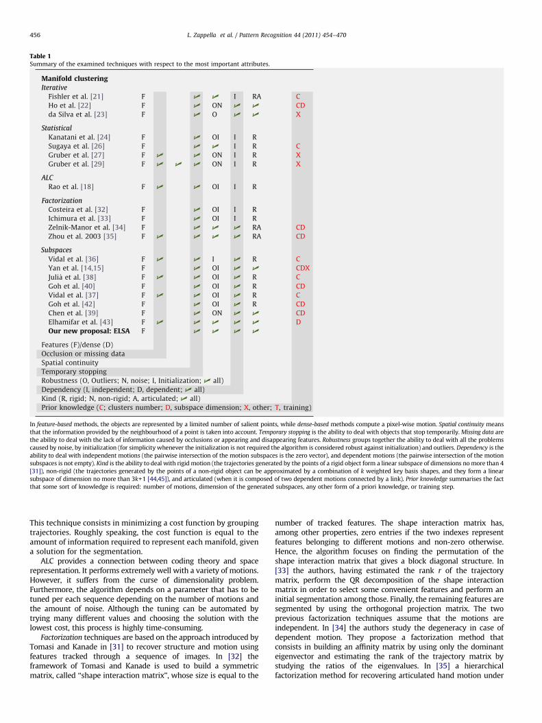
Table 1Summary of the examined techniques with respect to the most important attributes.

In feature-based methods, the objects are represented by a limited number of salient points, while dense-based methods compute a pixel-wise motion. Spatial continuity means

that the information provided by the neighbourhood of a point is taken into account. Temporary stopping is the ability to deal with objects that stop temporarily. Missing data are

the ability to deal with the lack of information caused by occlusions or appearing and disappearing features. Robustness groups together the ability to deal with all the problems

caused by noise, by initialization (for simplicity whenever the initialization is not required the algorithm is considered robust against initialization) and outliers. Dependency is the

ability to deal with independent motions (the pairwise intersection of the motion subspaces is the zero vector), and dependent motions (the pairwise intersection of the motion

subspaces is not empty). Kind is the ability to deal with rigid motion (the trajectories generated by the points of a rigid object form a linear subspace of dimensions no more than 4

[31]), non-rigid (the trajectories generated by the points of a non-rigid object can be approximated by a combination of k weighted key basis shapes, and they form a linear

subspace of dimension no more than 3k+1 [44,45]), and articulated (when it is composed of two dependent motions connected by a link). Prior knowledge summarises the fact

that some sort of knowledge is required: number of motions, dimension of the generated subspaces, any other form of a priori knowledge, or training step.

L. Zappella et al. / Pattern Recognition 44 (2011) 454–470456

This technique consists in minimizing a cost function by groupingtrajectories. Roughly speaking, the cost function is equal to theamount of information required to represent each manifold, givena solution for the segmentation.

ALC provides a connection between coding theory and spacerepresentation. It performs extremely well with a variety of motions.However, it suffers from the curse of dimensionality problem.Furthermore, the algorithm depends on a parameter that has to betuned per each sequence depending on the number of motions andthe amount of noise. Although the tuning can be automated bytrying many different values and choosing the solution with thelowest cost, this process is highly time-consuming.

Factorization techniques are based on the approach introduced byTomasi and Kanade in [31] to recover structure and motion usingfeatures tracked through a sequence of images. In [32] theframework of Tomasi and Kanade is used to build a symmetricmatrix, called ‘‘shape interaction matrix’’, whose size is equal to the

number of tracked features. The shape interaction matrix has,among other properties, zero entries if the two indexes representfeatures belonging to different motions and non-zero otherwise.Hence, the algorithm focuses on finding the permutation of theshape interaction matrix that gives a block diagonal structure. In[33] the authors, having estimated the rank r of the trajectorymatrix, perform the QR decomposition of the shape interactionmatrix in order to select some convenient features and perform aninitial segmentation among those. Finally, the remaining features aresegmented by using the orthogonal projection matrix. The twoprevious factorization techniques assume that the motions areindependent. In [34] the authors study the degeneracy in case ofdependent motion. They propose a factorization method thatconsists in building an affinity matrix by using only the dominanteigenvector and estimating the rank of the trajectory matrix bystudying the ratios of the eigenvalues. In [35] a hierarchicalfactorization method for recovering articulated hand motion under

L. Zappella et al. / Pattern Recognition 44 (2011) 454–470 457

weak perspective projection is presented. They consider each part ofthe articulated object as independent, and they use any techniqueable to deal with missing data to fill the gaps in the trajectorymatrix. In a second step, they guarantee that the extremities ofconsecutive objects are linked in the recovered motion.

Factorization techniques are based on a very simple andelegant framework. However, they are particularly sensitive tonoise and cannot deal very well with outliers. Moreover, most ofthe techniques assume rigid and independent motions.

The last category of manifold clustering is the subspace estimation

techniques. The work presented in [36] is one of them. First,exploiting the fact that trajectories of rigid and independent motiongenerate subspaces at maximum of dimension 4, they project thesetrajectories onto a five-dimensional space using PowerFactorization.Afterwards, the Generalized Principal Component Analysis (GPCA) isused to fit a polynomial of degree n, where n is the number ofsubspaces (i.e. the number of motions), to the data and estimate thebasis of the subspaces using the derivatives of the polynomial. Morerecently, the same authors extend in [37] the above-mentionedframework using RANSAC to perform the space projection in order todeal with outliers. Another well-known technique is the LocalSubspace Affinity (LSA) [14,15]. LSA is able to deal with differenttype of motion: independent, articulated, rigid, non-rigid, degenerateand non-degenerate. The key idea is that different motion trajectorieslie in different subspaces. Thus, the subspaces are estimated and anaffinity matrix is built using a measure based on principal angles. Thefinal segmentation is obtained by clustering the affinity matrix. One ofthe main limitation of LSA is that a full trajectory matrix withoutmissing data is assumed. In [38] a technique similar to LSA ispresented in order to deal with missing data. The idea is to fill themissing data so that the final matrix will have a frequency spectrumsimilar to the one of the input matrix. When a full trajectory matrix isobtained an affinity matrix is built and a cluster algorithm based onnormalized cuts is applied in order to provide the segmentation. In[39] the authors propose a generalization of LSA called SpectralCurvature Clustering (SCC). SCC differs from LSA for two mainreasons. The first reason is related to the affinity measure, as SCC usespolar curvature while LSA uses principal angles. The second reason ishow they select the points used to estimate the local subspaces: SCCuses an iterative random sampling, while LSA uses the nearestneighbours. A completely different strategy is presented in [40]where, starting from the Locally Linear Embedding algorithm [41],they propose the Locally Linear Manifold Clustering algorithm (LLMC).With LLMC the authors try to deal with linear and non-linearmanifolds. The same authors extended this idea to Riemannianmanifolds [42]. They project the data from the Euclidean space to aRiemannian space and reduce the clustering to a central clusteringproblem. More recently in [43] a new way for describing thesubspaces called Sparse Subspace Clustering (SSC) was presented. Theauthors exploit the fact that each point (in the union of subspaces)can be described with a sparse representation with respect to thedictionary composed of all the points. By using l1 optimisation, andunder mild assumptions, they estimate the subspaces and they builda similarity matrix which is used to obtain the final segmentation byspectral clustering.

Subspace estimation techniques can deal with intersection ofthe subspaces and do not need any initialization. However, allthese techniques suffer from common problems: curse ofdimensionality, a weak estimation of the number of motionsand of the dimension of the subspaces. The curse of dimension-ality is mainly solved in two ways: projection onto smallersubspaces or random sampling. Conversely, estimation of thenumber of motions and of the subspace dimension remain twopractical open issues.

Manifold clustering, specifically the group of subspace estima-tion, seems to be a good candidate for further investigation. This

group of techniques already provides a good performance interms of segmentation quality and it is naturally extended tostructure from motion algorithms. A quick glance at Table 1indicates that the price to pay for dealing with different kinds ofmotion and with dependent motions is a higher a priori knowl-edge (in particular about the dimension of the generatedsubspaces). Another common limitation that should be overcomeis the required knowledge about the number of motions in thescene.

Among the subspace estimation techniques reviewed,the Local Subspace Affinity method proposed by Yan and Pollefeys[14,15] appears a promising approach. As already concludedby Tron and Vidal in [17], for the case of non-missing dataLSA performs better than GPCA and a RANSAC based technique. Itis able to segment different types of motion (independent,dependent, articulated, rigid, non-rigid, degenerate and non-degenerate) as well as to deal with a limited amount ofmismatches in the tracked features. Furthermore, it is based ona relatively simple framework that can be easily extended toinclude more information and, despite its good performance,there is room for improvement, as explained in the next section.

3. Local Subspace Affinity (LSA)

The general idea of LSA is that trajectories that belong todifferent motions lie on different subspaces. Thus, the segmenta-tion can be obtained by grouping together all the trajectories thatgenerate similar subspaces. Following this idea, LSA estimates thesubspace generated by each trajectory and builds an affinitymatrix. The affinity measure between two trajectories is given bythe distance between the two generated subspaces. The finalsegmentation is obtained by clustering the affinity matrix.

3.1. The algorithm

LSA can be summarised in six fundamental steps:

1.

build a trajectory matrix W2f�p, where f is the number of framesof the input sequence and p is the number of tracked featurepoints;

2.

estimate the rank of W2f�p; this step is accomplished by amodel selection (MS) technique inspired by the work ofKanatani [46]:

r¼ argminr

l2rþ1Pr

i ¼ 1 l2i

þkr

!, ð1Þ

li being the i-th singular value of W2f�p, and k a parameter thatdepends on the noise of the tracked point positions: the higherthe noise level is, the larger the k should be [14];

3.

project every trajectory, which can be seen as a vector in R2f ,onto an Rr unit sphere by singular value decomposition (SVD)and truncation to the first r components of the right singularvectors;

4.

exploiting the fact that in the new space (global subspace)most points and their closest neighbours lie in the samesubspace, the local subspaces generated by each trajectory,and its nearest neighbours (NNs), are computed; this result canbe achieved by SVD, hence the estimation of the local subspacedimension is required again in order to truncate the SVDresult; such an estimation can be done by the same modelselection technique illustrated in formula (1);

5.

compute an affinity matrix A, where the affinity is a function ofthe distance between the local subspaces in terms of principalangles;

L. Zappella et al. / Pattern Recognition 44 (2011) 454–470458

6.

cluster A in order to have the final motion segmentation; anyclustering technique could be used, the authors suggestNormalized Cuts [47].

3.2. Problems

LSA provides an elegant solution for the manifold clusteringproblem, however, it is possible to identify some weaknesses ofthe algorithm.

The first weakness is that LSA is able to deal only with fulltrajectories, no missing data are allowed (step 1). This is animportant limitation, however, some authors have alreadypointed out possible solutions [38].

A second weakness is the fact that MS, formula (1), relies on aparameter k which has to be tuned depending on the noise leveland the number of motions (steps 2 and 4). Hence, MS requiresprevious knowledge regarding the amount of noise and thenumber of motions. Moreover, it is very sensitive to the parameterk, to the extent that Tron and Vidal, in their implementation ofLSA [17], claim that they had problems in finding a value for k thatwas good for all the sequences of the Hopkins155 database.Therefore, in [17] the authors avoided rank estimations andpreferred to fix the space size. They chose to fix the global spacedimension to 4n (step 2), where n is the number of motions. Theyalso fixed the dimension of the local subspaces generated by eachtrajectory to 4 (step 4). By doing so, only the number of motions isrequired. However, the ability of LSA to deal with different typesof motion is greatly reduced, in fact only rigid and non-degeneratemotions ensure a rank equal to 4 [31].

Another problem consists in the fact that Normalized Cutsdoes not provide a reliable instrument for estimating the numberof clusters (in the case of motions segmentation, a cluster isequivalent to a motion). Shi and Malik in [47] suggest to use theCheeger constant [48] or the cost of the last cut as an indication ofwhether or not it is worth to continue the cutting process.However, these two constants are highly sensitive to noise andthey require the use of thresholds that may change depending onthe input sequence. This is the reason why most of the availableimplementations of Normalized Cuts assume the final number ofclusters as known data.

4. Enhanced Local Subspace Affinity (ELSA)

Our proposed ELSA fixes the weaknesses of LSA as it findsautomatically a good value for k without requiring any a prioriknowledge, and introduces a robust estimation of the number ofmotions. In Section 4.1 the Enhanced Model Selection techniquefor rank estimation is presented and in Section 4.2 a robustnumber of motions estimation is described.

4.1. Enhanced Model Selection (EMS)

EMS automatically finds a good k value for formula (1), so thatthe amount of noise and the number of motions are not requiredas a priori knowledge. As formula (1) is used in steps 2 and 4 ofLSA, the estimated k for the global space (step 2) is called kg, whilethe k for the local subspaces (step 4) is called ks.

EMS is first applied to step 2 for the rank estimation of thematrix W2f�p. For the moment, the dimension of the local subspacegenerated by each trajectory is fixed to 4 (assuming the motionsare rigid), the extension of EMS to step 4 is explained later. Thekey idea of EMS lies in the relationship between the rank of W2f�p

estimated by MS (formula (1)), and the computed affinity matrix

A (step 5). To offer a pictorial understanding of such a relation-ship, an example is shown in Fig. 1(a)–(f), where the affinitymatrices, obtained after estimating the rank with different kg

values, are shown. A more rigorous explanation will be presentedin Section 4.1.1.

The sequence used in this example has three rigid motions(maximum rank is 12). When the rank of W2f�p is estimated usingan inappropriate kg value, the affinity matrix does not provide anyuseful information, as in Fig. 1(a) and (b) (rank overestimated)and Fig. 1(d)–(f) (rank underestimated). The best affinity matrix,visually speaking and knowing how many motions are in thescene, is obtained with kg¼10�7.5, which gives an estimated rankof 10, Fig. 1(c).

The relationship between the chosen kg and the computedaffinity matrix clarifies why a wrong choice of kg can greatly affectthe final segmentation. It is crucial for LSA to have a good rankestimation of the trajectory matrix in order to perform a correctsegmentation. On the other hand, this relationship is giving someinformation: by looking at the affinity matrix it is possible toassess the accuracy of the rank estimation. In Section 4.1.1 weanalyse why there is such a relationship, and in Section 4.1.2 weexplain that, without knowing the number of motions andwithout assuming any order of the tracked features, the entropycan be used as a measure of the ‘‘reliability’’ of the affinity matrix,and hence of the estimated rank. Moreover, in Section 4.1.3 aspeed up algorithm is proposed in order to quickly obtain anaffinity matrix with high entropy, avoiding an exhaustive searchamong a big range of kg values. Finally, the extension of EMS forthe estimation of the size of the local subspaces is presented inSection 4.1.4.

4.1.1. Affinity matrix as a function of the estimated rank

Before getting into details about how the relationship betweenthe affinity matrix and the estimated rank r (and hence the kg

value) could be exploited, let us analyse more deeply thebehaviour of the affinity matrix in relation to the estimated rankr. As there are many factors that influence the final affinity matrixit is easier to start with a simplified problem and extend it later tothe real case. Assume for the moment that there is no noise in thetracked feature positions, and that the ground truth set of NNs ofeach trajectory is known. Also, assume that the local subspacesgenerated by trajectories of different motions are orthogonal.

The affinity between two generic trajectories a and b dependson the distance between their local subspaces, which in LSA iscomputed through the principal angles. Let us recall that theprincipal angles between two subspaces SðaÞ and SðbÞ are definedrecursively as a series of angles 0ry1r , . . . ,ryM rp=2, whereM¼minfrankðSðaÞÞ,rankðSðbÞÞg [49]:

cosðy1Þ ¼ maxuASðaÞ,vASðbÞ

uT v¼ uT1v1, ð2Þ

while

cosðykÞ ¼ maxuA SðaÞ,vA SðbÞ

uT v¼ uTk vk, 8k¼ 2, . . .M, ð3Þ

s:t: : JuJ¼ JvJ¼ 1, uT uj ¼ 0, vT vj ¼ 0 8j¼ 1, . . . ,k�1:

The vectors u1, . . . ,uk and v1, . . . ,vk are the principal vectors. In theideal case and with a perfect rank estimation, the principal anglesyi between two local subspaces generated by trajectories of thesame motion should be 0. On the other hand, when a and b belongto different motions, yi should be close to p=2. Let us nowdiscuss the behavioural trend of the principal angles as a functionof r (the rank of the global subspace) in the cases of under andoverestimation.

The analysis in the case of underestimation is quite easy todevelop. In fact, in this case the components of the lost

Fig. 1. Affinity matrices computed with different kg values; real sequence 1R2RC from the Hopkins155 database, theoretical maximum rank of W is 12; black is minimum

affinity, white is maximum affinity and r is the estimated rank. (a) kg¼10�12; r¼57; (b) kg¼10�10; r¼21; (c) kg¼10�7.5; r¼10; (d) kg¼10�6; r¼6; (e) kg¼10�5; r¼5;

(f) kg¼10�4; r¼4.

L. Zappella et al. / Pattern Recognition 44 (2011) 454–470 459

dimensions are projected onto the remaining dimensions, artifi-cially forcing the two local subspaces towards each other to thepoint when they collapse onto exactly the same local subspace. Asa consequence, two local subspaces tend to become closer as r

decreases.On the other hand, the behaviour of principal angles when r is

an overestimation is less intuitive. In fact, in [50] it is explainedthat the problem of computing principal angles and principalvectors when the rank of the global space is overestimated is anill-posed problem. To the authors’ knowledge, the most helpfulmathematical result for the case under analysis is presented in[51]. The authors study the probability density function (pdf) ofthe largest principal angle between two subspaces chosen from auniform distribution on the Grassmann manifold of p-planesembedded in Rn. They show that, when n is appreciably biggerthan p (precisely n42p�1), the pdf is close to zero for smallangles and rapidly increases to reach a global maximum in p=2.

The resemblance between this abstract mathematical situationand the practical case under analysis is represented by the fact that,when the rank is overestimated, the extra component added to thetrajectory vectors (in the global space) are sampled from basisvectors of the null space of W. In fact, the projection onto the globalspace is done as follows. The matrix W2F�N is decomposed by SVDas: W¼ UDVT . Hence, if the rank of W is rreal, the first rreal columns ofV correspond to the basis of the row space of W whereas theremaining N�rreal columns of V correspond to the basis of the nullspace of W. In this new global subspace the first rreal components ofeach row i of V (for i¼[1,N]) represent the trajectory i in the globalsubspace. In Fig. 2(a) the meaning of each column and row of V issummarised in the case that the estimated rank of W is rest¼rreal.However, if the estimated rank of W is rest 4rreal, each trajectory i

will be represented by its true rreal components (taken from thefirst rreal components of row i of matrix V) plus rest�rreal extracomponents that are taken from row i of the rest�rreal basis of thenull space of W. These extra components are unrelated to thetrajectory i, hence they are random with respect to that trajectory.This second case is summarised in Fig. 2(b). Note that theprojection of the trajectories onto the global space is oblique, forthis reason the components that exceed the real rank are noteliminated and they act as random values.

Finally, note that all of the reasoning holds true even in thecase of no noise and it does not involve the selection of the NNs.Hence, when rest is sufficiently big the work of [51] applies to thecase under analysis. Therefore, the higher the overestimation, thecloser the resemblance to a uniform distribution.

From the result presented in [51], an overall increasing

behaviour of the principal angles as a function of the estimatedrank can be inferred.2 To support this inference, in Fig. 3(a)–(d) we

2 To the authors’ knowledge, no information is known about the precise

analytical behaviour of such functions.

present the trend of the largest principal angle of syntheticsequences with 2 rigid motions (hence the maximum rank is 8)and no noise. As the test is performed using the first part of theLSA algorithm the nearest neighbours (NNs) are estimated asexplained in step 4 of the LSA summary (Section 3.1). For eachsequence four angles are compared: two angles betweentrajectories of the same motion (blue lines) and two anglesbetween trajectories of different motions (red lines). These resultsare just a few samples of a large number of experimentsperformed on the whole synthetic database (see Section 5.1 fora detailed description of the 240 synthetic sequences) with 2, 3, 4and 5 rigid motions and an increasing noise level and on theHopkins155 database. All the experiments show the same pattern,i.e. when the rank is very small all principal angles tend towardszero, while when the rank is heavily overestimated all of theangles tend towards p=2. For simplicity, only the largest principalangle is shown in the examples. However, the smaller angles alsofollow the same trend. These experiments confirm the overallincreasing behaviour inferred from [51]. Moreover, from Fig. 3(a)to (d) it is possible to appreciate that when the estimation of therank is close to the correct rank, then the principal angles betweenlocal subspaces generated by trajectories of different motions arehigher than those between local subspaces generated by trajec-tories of the same motion.

From now on, we will refer to the behaviour of the principalangles yi with respect to r as the function yiðrÞ. Let us now analysehow this behaviour reflects on the affinity value between twofixed generic trajectories a and b, where the affinity is defined as

AðrÞ ¼ e�PM

i ¼ 1sin2ðyiðrÞÞ: ð4Þ

In the ideal case and with a perfect rank estimation, the affinitybetween trajectories of the same motion is maximum (i.e. 1),whereas the affinity between trajectories of different motions isminimum (i.e. close to 0). Similarly to what was done for theprincipal angles, it is interesting to understand the globalbehaviour of the function A(r). In order to do so, we study thefirst derivative of A(r):

dAðrÞ

dr¼�e�

PM

i ¼ 1sin2ðyiðrÞÞ

XMi ¼ 1

2sinðyiðrÞÞcosðyiðrÞÞyiuðrÞ: ð5Þ

All of the functions appearing in the derivative (5) are non-negative for all values of r, except for yiuðrÞ (the first derivative ofyiðrÞ). However, it has been shown that yiðrÞ is overall increasing,so yiuðrÞZ0 for the majority of the values of r. The presence of theminus sign implies that dAðrÞ=drr0 for the majority of the valuesof r, i.e. A(r) has an overall decreasing behavior. Specifically, whenr is an underestimation all the affinity values tend to themaximum value, whereas when r is an overestimation they tendto the minimum value. Fig. 3(i)–(l) shows the affinity values of thesame pairs of trajectories used in Fig. 3(a)–(d), confirming theresults of the analysis just performed.

Fig. 2. Pictorial description of what happens when the rank of the global space is estimated. traji stands for the ith trajectory. (a) Ideal case; (b) real case.

L. Zappella et al. / Pattern Recognition 44 (2011) 454–470460

So far we have considered the case without noise and withperfectly orthogonal local subspaces. The effect of the presence ofnoise and the estimation of the NNs is that there may beoscillations in the functions of the principal angles (as in Fig. 3(e)–(h)), and so, potentially, also in the affinity functions. However,we will show later in this subsection why this, in turn, does notlead to big oscillations of the affinity values (as in Fig. 3(m)–(p)).

The last simplification was to consider orthogonal localsubspaces. Usually, in real sequences the local subspaces are notperfectly orthogonal. The effect of non-perfect orthogonality isthat, even in the overestimation cases, some pairs of trajectoriesmay have low affinity but not exactly equal to zero. The effects ofnon-perfect orthogonality and of the estimation of the NNs can beseen in Fig. 3(a)–(d): despite the fact that there is no noise, it ispossible to notice small oscillations in the yiðrÞ.

Therefore, the main consequence of moving from an ideal to areal situation is that the yiðrÞ may have wider oscillations.However, such oscillations rarely lead to oscillations of theaffinity values. In fact, the oscillations of the principal anglesmay be compensated by the sum involved in the computation ofthe affinity, formula (4) (especially if the oscillation affects oneof the smallest angles). Moreover, the highly non-linear behaviourof the decreasing exponential used to define the affinity, tends tosmooth the effect of small changes. Even in the worst casescenario, it is very unlikely that all the affinities between the pairsof trajectories oscillate in correspondence to the same estimationof the rank. Hence, it is highly probable that the trend of A(r)remains overall decreasing. Let us stress that Fig. 3(m)–(p) testifythat, even when the presence of noise induces considerableoscillations in the yiðrÞ, the affinities are not dissimilar to those ofthe case without noise (Fig. 3(i)–(l)).

Summarising, even without the assumptions made at thebeginning, the affinity between every pair of trajectories ismaximum when the rank of the global subspace is highlyunderestimated and is minimum when the rank is highlyoverestimated. In between, the affinities have a decreasing trend.Specific pairs may present oscillations, but the majority of theaffinities remain, overall, decreasing functions of r.

4.1.2. How to choose a good affinity matrix

Now that the relationship between the affinity and theestimated rank has been clarified, it is necessary to find a measureof the ‘‘reliability’’ of the affinity matrix. The ideal criterion for theselection of the affinity would be to choose the one thatminimises the final misclassification rate. However, the groundtruth of the segmentation is not always known. In real cases a

convenient criterion could be to choose a high contrasted affinitymatrix, because the higher the contrast the higher the quantity ofinformation that can be used to compare the trajectories. A wellknown measure of contrast, and of quantity of information, is theentropy [52]:

EðAðrÞÞ ¼�X1

i ¼ 0

hAðrÞðiÞ log2ðhAðrÞðiÞÞ, ð6Þ

where hAðrÞðiÞ is the histogram count in the bin i (in ourexperiments we use 256 bins). As stated in the previous section,when r is an underestimation, all of the affinities tend to beclustered around 1, leading to a very low entropy value. As r

approaches the correct rank, the affinities between trajectories ofthe same motion tend to diverge from those between trajectories ofdifferent motions, hence the entropy increases. Note that it is notpossible to exclude that theoretically the entropy function can haveoscillations, but regardless we are more interested in its overallbehaviour. The more r is increased, becoming an overestimation,the more the affinities tend to converge around 0, consequently theentropy decreases again. Fig. 3(q)–(t) shows the trend of theentropy for the same synthetic sequences used to show yiðrÞ

(Fig. 3(e)–(h)) and A(r) (Fig. 3(m)–(p)) in the presence of noise.Similarly, Fig. 4 shows the entropy trend of the real sequence1R2RC (Hopkins155 database) used to compute the affinitymatrices shown in Fig. 1.

Notice that the entropy would not be maximum in the case of aperfect affinity matrix with only two values (maximum andminimum). However, such a situation is extremely rare in realsequences. Also in synthetic sequences with no noise a perfectaffinity matrix is obtained only when the motions are completelyindependent. In practical cases, without having a clear indicationabout which affinity matrix is the most suitable, the highestentropy choice has the interesting property of discarding uniform(and thus useless) affinity matrices. In the examples shown inFig. 3(q)–(t) the highest entropy always corresponds to a rankvalue where the affinities between trajectories of the samemotion are higher than those between trajectories of differentmotions (Fig. 3(m)–(p)). In the example of Fig. 4 the maximumcorresponds to the affinity matrix of Fig. 1(c), which is the onecorresponding to the rank estimation closest to the real rank. Wecall the Enhanced Model Selection (EMS) this new way ofestimating the rank as the one that leads to the affinity matrixwith the maximum entropy.

As stated before, it is not possible to ensure that the affinitymatrix with the maximum entropy corresponds to a perfect

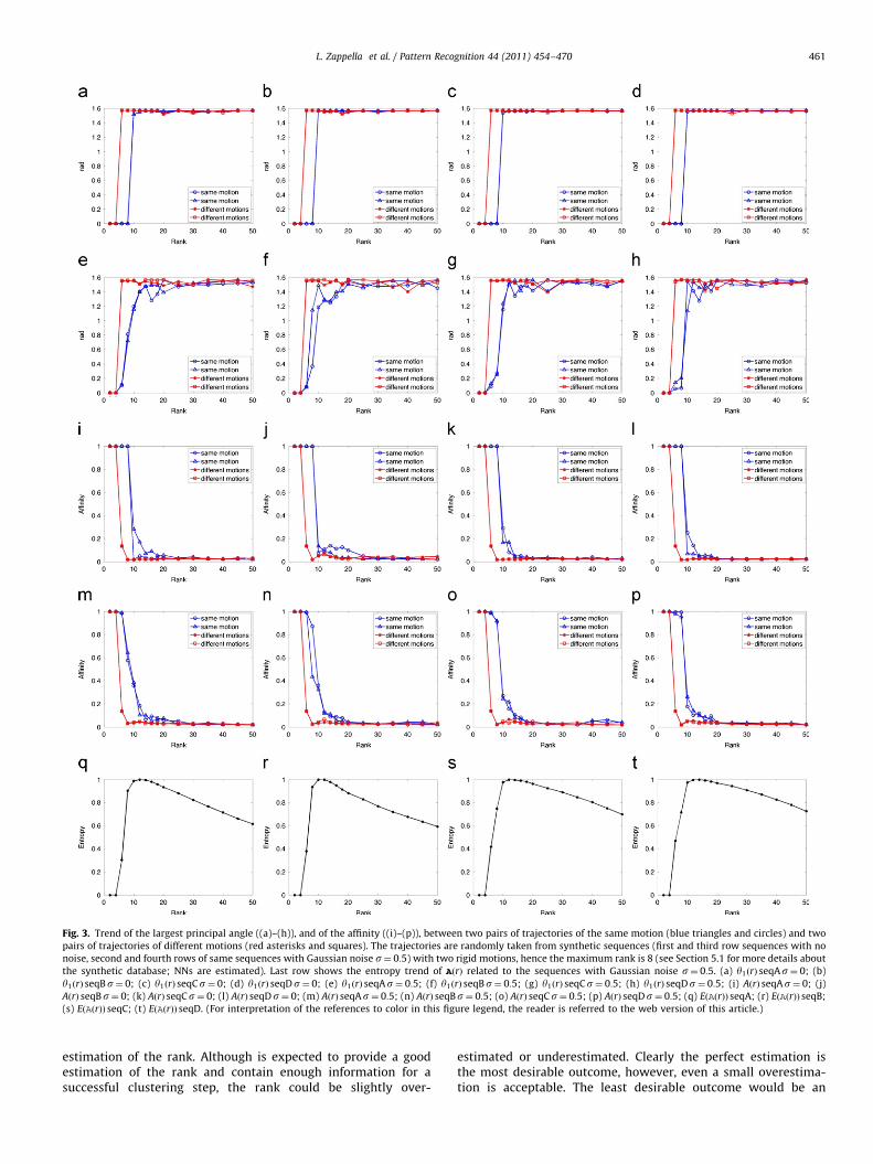
Fig. 3. Trend of the largest principal angle ((a)–(h)), and of the affinity ((i)–(p)), between two pairs of trajectories of the same motion (blue triangles and circles) and two

pairs of trajectories of different motions (red asterisks and squares). The trajectories are randomly taken from synthetic sequences (first and third row sequences with no

noise, second and fourth rows of same sequences with Gaussian noise s¼ 0:5) with two rigid motions, hence the maximum rank is 8 (see Section 5.1 for more details about

the synthetic database; NNs are estimated). Last row shows the entropy trend of AðrÞ related to the sequences with Gaussian noise s¼ 0:5. (a) y1ðrÞ seqAs¼ 0; (b)

y1ðrÞ seqBs¼ 0; (c) y1ðrÞ seqCs¼ 0; (d) y1ðrÞ seqDs¼ 0; (e) y1ðrÞ seqAs¼ 0:5; (f) y1ðrÞ seqBs¼ 0:5; (g) y1ðrÞ seqCs¼ 0:5; (h) y1ðrÞ seqDs¼ 0:5; (i) AðrÞ seqAs¼ 0; (j)

AðrÞ seqBs¼ 0; (k) AðrÞ seqCs¼ 0; (l) AðrÞ seqDs¼ 0; (m) AðrÞ seqAs¼ 0:5; (n) AðrÞ seqBs¼ 0:5; (o) AðrÞ seqCs¼ 0:5; (p) AðrÞ seqDs¼ 0:5; (q) EðAðrÞÞ seqA; (r) EðAðrÞÞ seqB;

(s) EðAðrÞÞ seqC; (t) EðAðrÞÞ seqD. (For interpretation of the references to color in this figure legend, the reader is referred to the web version of this article.)

L. Zappella et al. / Pattern Recognition 44 (2011) 454–470 461

estimation of the rank. Although is expected to provide a goodestimation of the rank and contain enough information for asuccessful clustering step, the rank could be slightly over-

estimated or underestimated. Clearly the perfect estimation isthe most desirable outcome, however, even a small overestima-tion is acceptable. The least desirable outcome would be an

Fig. 4. Example of the entropy trend experienced with all the sequences used in

the experiments. This specific example refers to the same sequence used to show

the affinity matrices in Fig. 1.

Fig. 5. Error of EMS rank estimation with different number of motions and noise

levels. Each point is given averaging the errors over 10 different sequences.

L. Zappella et al. / Pattern Recognition 44 (2011) 454–470462

underestimation as this corresponds to cutting important in-formation. In Fig. 3(i)–(p) it can be appreciated how all theaffinities go to 1 very quickly when the rank is underestimated.

In order to prevent a possible underestimation, or reduce itseffects, it may be safer to increase the estimated rank by a smallamount. Our experiments have shown that there is a correlationbetween the number of motions (or the amount of noise) and theposition of the maximum entropy: the greater the number ofmotions (or the higher the noise) the lower the estimation of therank. In Fig. 5 the error of the EMS rank estimation is shown inrelation to the number of motions and the noise level. Theseresults are computed on the synthetic database described inSection 5.1, each point in the plot corresponds to the average errorover 10 synthetic sequences for each number of motion and eachnoise level. As can be seen, when the number of motions increasesthe error of the EMS rank estimation tends towards negativevalues. Similarly, the higher the noise the lower the rankestimation. We leave as a matter of further investigation a properunderstanding of this behaviour. As a preliminary study, apossible way to correct the estimated rank could be to add 1size for each motion to the previously EMS estimated rank. Byadding only 1 size for each motion, even if the maximum wasalready an overestimation or a perfect estimate, the correctiondoes not introduce too much random information, whereas if themaximum was an underestimation some important informationis added.

EMS with correction is called EMS+, in Section 5 theperformances between EMS and EMS+ are compared.

4.1.3. How to speed up the choice

We propose here a speed up technique that can be used inorder to quickly find an affinity matrix with a high entropy. Inorder to have a fast but good estimation of the rank, we exploitthe concavity of the overall entropy behaviour. As explained in theprevious section, the entropy may have oscillations. However, bytaking opportune safety measures it is possible to quickly find anaffinity matrix with an entropy very close to the highest value.One can always renounce to speed in favor of a better estimation,however, in Section 5 we show that even with this approximated(but faster) choice good results are obtained.

Assuming that there may be small oscillations in the entropyfunction, in order to avoid to select a local maximum it issufficient to use a large sampling step (in our experiments thestep Dkg ¼ 1=

ffiffiffiffiffiffi10p

). Moreover, to establish the gradient of theentropy we do not choose only 2 samples but 3. By doing so, whena minimum is encountered we can extend the sampling towards

the two extremes until a choice can be made. Once the gradient isestablished, we shift our search towards the increasing gradientrepeating the sampling process until the maximum is found. Wewould like to remark that in our experiments when the entropywas sampled in the way just explained we have not found anyfluctuations in its trend. However, when the entropy is computedwith a finer sampling step, in some sequences a very smalloscillation may be found close to the maximum values. On thewhole Hopkins155 database an oscillation can be found only inthe following sequences: 1RT2TC_g13, 2R3RTCRT, 2T3RCTP,articulated, cars1 and cars8. As shown in Fig. 6 the oscillationsare very small and occur very close to the maximum entropyanyway. Hence, even if in these few cases our algorithm hadselected a local maximum, the built affinity matrices would havehad a very high entropy.

Of course, one can always argue that there may be aparticularly unlucky situation where the combination of badestimation of NNs and noise generates a very big oscillation, tothe point that even with the kind of sampling just described, ouralgorithm would choose a local maximum. However, the oscilla-tions are more likely to be around the correct rank, hence there isa chance that the selected affinity matrix can provide enoughinformation anyway. Moreover, in such extreme conditions theassumptions of the LSA framework would probably be violatedleading to bad segmentation even if the rank is perfectlyestimated.

4.1.4. Size estimation of the local subspaces

So far we have assumed that the size of the local subspaces(step 4) was fixed to 4. Once, the value kg has been found equal to1/10x, ks can be set to 1=

ffiffiffiffiffiffiffiffi10xp

. This corresponds to the choicemade by the authors of LSA. In fact, Yan and Pollefeys explain in[14] that when detecting the rank of the local subspaces, due to asmall number of samples, the noise level is higher, so it isdesirable that ks4kg .

In summary, EMS and EMS+, by exploiting the relationshipbetween the rank estimation of the trajectory matrix and theaffinity matrix, are able to automatically tune the value of k forthe global and local dimension estimation without requiringknowledge about the number of motions nor the amount of noise.Better rank estimations result in a better motion segmentationand, as EMS and EMS+ do not make any assumption regarding thetypes of motion, it can be used under any condition.

4.2. Number of motions estimation

Another weakness of LSA is related with the final segmentationof the affinity matrix. Yan and Pollefeys in [14] suggest to use

Fig. 6. The only entropy trend with oscillation found on the whole Hopkins155 database. In these plots the rank was sampled from 2 to 20 with a step of 2, from 20 to 50

with a step of 5. (a) 1RT2TC_g13; (b) 2R3RTCRT; (c) 2T3RCTP; (d) articulated; (e) cars1; (f) cars8.

L. Zappella et al. / Pattern Recognition 44 (2011) 454–470 463

Normalized Cuts [47]. Normalized Cuts is a good solution as longas the number of motions is known. When this information is notavailable, at every iteration the decision to terminate the processor not has to be taken. The authors of Normalized Cuts suggest touse the Cheeger constant [48] or the cost of the last cut in order totake this decision. The Cheeger constant and the cost of the lastcut are both clues of how difficult it is to split the graph byremoving a specific edge. When, after finding the minimum cut,one of these two values is high it means that it is not worthsplitting the graph and the process can stop. Therefore, theseindicators need a threshold to decide when the value is ‘‘highenough’’. The problem is that such a threshold is stronglyinfluenced by the noise level and the number of motions. Thisexplains why most of the Normalized Cuts implementationsrequire to know in advance the number of motions.

Having tested the difficulty of using the Cheeger constant or thecost of the last cut, we try a different way, exploiting some spectralgraph theory theorems. Specifically the following proposition.

Proposition 1 (Number of connected components). Let G be an

undirected graph with non-negative weights. Then, the multiplicity n

of the eigenvalue 0 of the Laplacian matrix equals the number of

connected components in the graph [54].

In [47] it is shown that finding the minimum cut for splittingthe graph, is equivalent to thresholding the values of the secondsmallest eigenvector of the Laplacian matrix L:

L¼ D�A, ð7Þ

where A is the adjacency matrix (specifically, in our case it is theaffinity matrix), and D is a p� p diagonal matrix, p being thenumber of tracked features. Every entry Dði,iÞ contains the sum ofthe weights that connect node i to all of the others. Hence, matrixL and Proposition 1 could be used in order to estimate the numberof motions. Proposition 1 refers to an ideal case where theeigenvalues that correspond to the connected components are

exactly equal to 0 (which means no noise and fully independentmotions). However, perturbation theory says that if there is not anideal situation the last n eigenvalues are not equal to 0,nevertheless they should be very close to those of the ideal case[54]. Naturally, in motion segmentation, especially with realsequences, the ideal situation is not expected, but theoretically itshould be possible to identify the threshold between theeigenvalues that correspond to the connected components andthe remaining eigenvalues.

Proposition 1 holds true also when using the eigenvaluespectrum of the Symmetric Normalized Laplacian matrix Lsym

[54,55] instead of the Laplacian matrix L:

Lsym ¼ D�1=2LD�1=2: ð8Þ

Fig. 7 shows the eigenvalues of L (first row) and of Lsym (secondrow) of a synthetic sequence with 3 motions and with anincreasing noise level. The last three eigenvalues, which shouldsuggest the number of motions, are plotted with a red filled circle.In the plots all the eigenvalues are normalized in order to allow aneasier comparison between L and Lsym. As can be seen, when thenoise increases the difference between the red filled eigenvaluesand the others decreases. However, the difference between thefourth to last and the third to last eigenvalues remains ratherlarge in the Lsym spectrum, while it becomes really small in the L

spectrum. In the next section the experimental results of theestimation of the number of motions using L and Lsym arecompared.

As was previously stated, when the Cheeger constant or the cost ofthe last cut are used, the main problem is the choice of a threshold.The same problem is present when using the spectrum of theeigenvalues, regardless of the choice of L or Lsym. However, while withthe Cheeger or the cost of the last cut there is not much informationthat can be used in order to take such a decision, with the eigenvaluesthe information of the whole spectrum can be used. Nevertheless, the

L. Zappella et al. / Pattern Recognition 44 (2011) 454–470464

threshold cannot be fixed as the noise greatly influences the distancebetween the eigenvalues, as shown in Fig. 7. In order to dynamicallyfind a threshold for every case we try different techniques. In general,estimating the number of motions using the eigenvalue spectrum canbe seen as a two class classification problem: class 1 is the class of theeigenvalues above the threshold while class 2 is the class of theeigenvalues below the threshold. The number of eigenvalues insideclass 2 is the estimation of the number of motions. The first techniquethat we test is the Fuzzy C-Means clustering (FCM) [56]. Thistechnique returns a probability of belonging to class 1 and to class 2for every element of the set. The second technique is Otsu’s method[57] which chooses the threshold to minimise the intra-class variance.As in this particular case it seems that the inter-class variance is alsoplaying an important role, we try to find a trade-off between theintra- and the inter-class variance. We take inspiration from theLinear Discriminant Analysis (LDA) which minimises the intra-classvariance while maximising the inter-class variance. With LDA thechosen threshold t is given as

argmaxt

Q1ðm1ðtÞ�mallÞ2þð1�Q1Þðm2ðtÞ�mallÞ

2

Q1s21ðtÞþð1�Q1Þs2

2ðtÞ, ð9Þ

where m1 and s1 are the mean and the variance of class 1 given acertain threshold t, m2 and s2 are the mean and the variance of class2, and mall is the mean of all the eigenvalues. In the originalformulation of LDA, Q1 is the probability of belonging to class 1.However, in this context this probability is unknown (knowing theprobability means knowing already the number of motions). At thesame time, not providing any weight for the two classes would meanthat both classes are equally likely even though this is not true.Therefore, Q1 should be seen as weight that has to favour class 1 overclass 2.

The nominator of formula (9) measures the inter-classdissimilarity, whereas the denominator measures the intra-class

Fig. 7. Eigenvalues spectrum of L (fist row) and of Lsym (second row) for a synthetic se

increasing Gaussian noise level. (a) L, snoise ¼ 0:0; (b) L, snoise ¼ 1:5; (c) L, snoise ¼ 3:0;

dissimilarity. Therefore, choosing the threshold that maximisesthis ratio is like choosing the threshold that maximises the inter-class dissimilarity and minimises the intra-class dissimilarity.

In the next session, one of the experiments presented is aboutthe estimation of the number of motions using the eigenvaluespectrum of L and of Lsym, and thresholding them with FCM, OTSUand LDA.

5. Experimental results

5.1. Databases

In order to evaluate ELSA, we perform different tests with realsequences. The database used is the Hopkins155 which is areference database for motion segmentation, composed of 155real video sequences: 120 with 2 motions and 35 with 3 motions.An example of two real sequences are shown in Fig. 8(a) and (b).Inside the Hopkins155 database there are different types ofsequences: checkboards, traffic and articulated/non-rigid. Thecheckboard is the main group (104 videos) thus it is likely that thetype and the amount of noise inside the database does not changemuch as most of the sequences are taken in the same environ-ment. For the purpose of testing the ELSA with bigger noisechanges, we create another six databases derived from theHopkins155 adding random Gaussian noise, with standarddeviations of 0.5, 1, 1.5, 2, 2.5 and 3 pixels, to the tracked pointpositions. The original database plus the six derived from itcompose a bigger database with 1085 video sequences.

Besides the Hopkins155 database, we also use a syntheticdatabase. Specifically, synthetic sequences composed of 50 frames,with rotating and translating cubes. Each cube has 56 trackedfeatures. An example of a synthetic frame (for plotting reasons withjust a few tracked features) is shown in Fig. 8(c). Similarly to what we

quence (similar to the one in Fig. 8(c)) with 3 rotating and translating cubes and

(d) Lsym , snoise ¼ 0:0; (e) Lsym , snoise ¼ 1:5; (f) Lsym , snoise ¼ 3:0.

L. Zappella et al. / Pattern Recognition 44 (2011) 454–470 465

did for the Hopkins155 we create also six derived databases addingnoise with different standard deviations (from 0.5 to 3 pixels) to theoriginal database for a total of 240 synthetic sequences. Syntheticsequences with 2 motions have been previously shown in Section4.1.1 in order to provide some examples of the trends of the principalangles, the affinity values and the entropy as functions of r. Sequenceswith 2, 3, 4 and 5 motions have been used in Section 4.1.2 in order toprovide some evidences of the correlation between the number ofmotions (or the noise level) and the rank estimated by EMS.Sequences with 3 motions have been used in Section 4.2 to showthe differences between the eigenvalue spectrum of L and Lsym.Finally, in Sections 5.3 and 5.5 we use sequences with 4 and 5motions to test the estimation of the number of clusters and ELSAalgorithm in a more challenging context.

5.2. Evaluation of the Enhanced Model Selection

In Section 4.1 it is explained how EMS is able to automaticallyadjust the parameter k to different noise conditions and differentnumber of motions in the sequence. In this section the results ofthe misclassification over the Hopkins155 database, and theHopkins155 database with extra noise, are shown. In these firstsets of experiments the knowledge about the number of motionsis assumed so that it is possible to assess the model selectiontechniques (MS, EMS and EMS+) independently from the accuracyof the estimation of the number of motions.

To evaluate the model selection the results of ELSA with EMSand ELSA with EMS+ are compared with the results obtainedwith: LSA fixing the global subspace size to 5 and 4n (where n isthe number of motions), LSA estimating the global subspace sizewith MS using the best k per each sequence (i.e. the k thatprovided the lowest misclassification rate per each sequence onthe original Hopkins155 database), and LSA with MS using theoverall best k (i.e. the k value, common for the whole database,that provided the lowest mean misclassification on the originalHopkins155 database). For all the algorithms the Recursive Two-Way Ncut [47] is used for the final clustering (this is why for 0extra noise level the LSA 5 and 4n results are slightly differentthan the ones in [17] where the clustering algorithm used was k-means with multiple restarts). We perform two set of experi-ments: the first is performed fixing the subspace sizes to 4, whilethe second is performed estimating both global and localsubspace sizes.

In Fig. 9 the results obtained fixing the subspace sizes to 4 areshown. With no additional noise (noise level equal to 0 in thegraphs, i.e. the original Hopkins155 database) the highest mis-classification is obtained when the global subspace size is fixed to5, this happens because a dimension of 5 corresponds for most ofthe global subspaces to a considerable underestimation of theirsize. The performances of LSA with best overall k, best k

per sequence, and fixing the global subspace to 4n are very similarto each other, however, when the noise increases the MS tends to

Fig. 8. Example of two input frames and the trajectories of real sequences from th

(b) checkboards; (c) synthetic.

fail (as it was tuned for the original Hopkins155) proving that MS isvery sensitive to noise. ELSA, both with EMS and EMS+, performsbetter than any other technique, with EMS+ proving to be moresolid than EMS when the number of motions increases. ELSAperforms better than MS with best k per sequence even on theoriginal database. This may seem counterintuitive as one wouldexpect that the best k per sequence leads to the best misclassifica-tion rate. However, it has to be remembered that the best k valueswere computed when also the local subspace sizes were estimatedand not fixed to 4. This small difference clearly changes which arethe best k values that have to be used and shows, once again, howunstable the MS is. When the noise level increases EMS and EMS+perform better than MS because they are able to adapt auto-matically to the different conditions. Moreover, ELSA performsbetter than LSA 4n because when the global subspace size is fixedto 4n the motions are considered rigid and fully independent evenwhen this is not true. Overall, this results show that a good modelselection allows to obtain better results than fixing the globalsubspace size. However, model selection is also very sensitive tothe noise and it requires a manual tuning in order to copesuccessfully with different noise levels.

The following set of experiments is obtained estimating alsothe local subspace sizes (as LSA 4n and 5 do not use anyinstrument to estimate the global subspace size they are notincluded in this set of experiments). The results are shown inFig. 10. As expected, with the original Hopkins155 database thelowest misclassification is obtained when the k is manually tunedfor each sequence. As expected, EMS and EMS+ perform worsethan MS with the best k per sequence, however, they do betterthan MS with the best overall k. As soon as extra noise is added,the misclassification of both MS strategies rises drasticallywhereas EMS and EMS+ are able to tune k automatically in orderto reduce the effects of the noise. As in the previous set ofexperiments, the misclassification rate of ELSA with EMS+ is lowerthan that of ELSA with EMS. With 2 motions the performances arevery similar. However, with 3 motions the compensation strategyplays an important role. In fact, without extra noise ELSA withEMS+ has performances very close to the one of LSA with best k

per sequence. In general ELSA with EMS+ misclassification rate isaround 6% lower than the misclassification of ELSA with pureEMS. If the plots of Figs. 9 and 10 are compared it is possible tonotice that, given a technique, the misclassification when the localsubspace sizes are estimated are almost always better than whenthe local subspace sizes are fixed to 4. Such a result shows thatalso a correct estimation of the size of the local subspaces plays a(minor) role in providing a better segmentation.

In summary, these results show that EMS and EMS+ are able toprovide a good estimation of the rank of the trajectory matrix inan automatic fashion. They do not require any a priori knowledgeand are able to deal successfully with different noise levels. As it isnot necessary for EMS and EMS+ to know in advance anysubspace dimension, they are able to deal with different types of

e Hopkins155 database and one frame from a synthetic sequence. (a) Traffic;

Fig. 9. Mean misclassification rate versus noise level for Hopkins155 databases (local subspace sizes are fixed to 4). (a) 2 motions; (b) 3 motions; (c) 2 and 3 motions.

Fig. 10. Mean misclassification rate versus noise level for Hopkins155 databases (local subspace sizes are estimated). (a) 2 motions; (b) 3 motions; (c) 2 and 3 motions.

L. Zappella et al. / Pattern Recognition 44 (2011) 454–470466

motion, which is not possible when the subspace size is fixed.Moreover, despite the fact that ELSA with EMS already providesvery good results, the simple correction strategy of EMS+ allowsto reach even better performances.

5.3. Estimation of the number of motions

The aim of ELSA is to be completely automatic withoutrequiring any a priori knowledge. Therefore, the next step is totest the estimation of the number of motions. As explained inSection 4.2, we test different thresholding techniques in order toperform the estimation exploiting the eigenvalues spectrum ofeither the Laplacian matrix L or the Symmetric NormalizedLaplacian Lsym. In both cases the Laplacian matrices are built afterEMS has been used in order to estimate the dimension of theglobal space. Concerning the setting of the thresholding algo-rithms, we tried different values and we present here the set thatobtains the best results on a random subset of the Hopkins155database (70 sequences). For the estimation using FCM, the bestresults are obtained by counting the eigenvalues with aprobability of belonging to class 2 equal to or greater than 0.9.For OTSU the best results are obtained using only the last 20eigenvalues. For LDA the best results are obtained with Q1¼0.8.

A first qualitative study suggests that Lsym is more robustagainst noise, as previously shown in Fig. 7. We run also aquantitative test estimating the number of motions on theHopkins155 database using both L and Lsym with the thresholdingtechniques explained in the previous section. Table 2 shows themean and variance of the error of the estimated number ofmotions for the tested thresholding techniques (the absolutevalue of the error is considered). As expected, regardless oftechnique, mean and variance are always considerably smallerwhen using Lsym than when using L. As the Symmetric Normal-

ized Laplacian spectrum seems to be more robust against noise,we choose Lsym in order to estimate the number of motions.

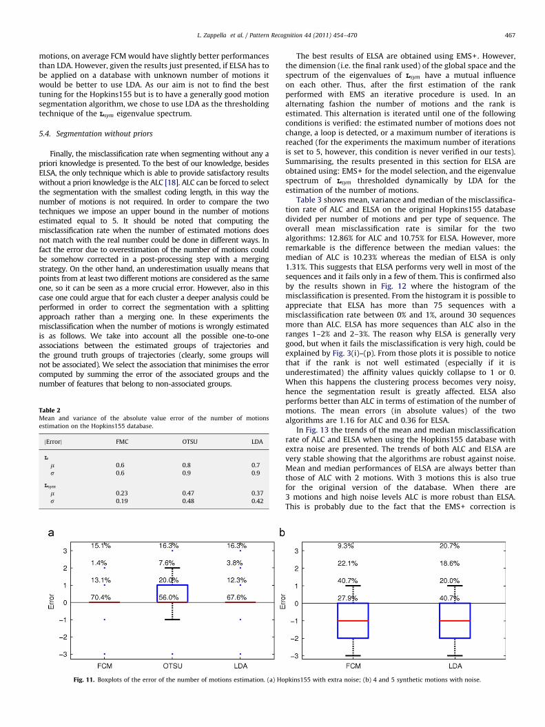
From the results of Table 2, OTSU seems to be the weakestmeasure. This is confirmed also when the same test is performedon the Hopkins155 with extra noise, as shown in Fig. 11. Thenumbers on each boxplot correspond to the percentage ofsequences where the error in the number of cluster estimationwas (from bottom to top) 0, 71, 72 or greater than 2 (inabsolute value). From these boxplots it is possible to see that FCMand LDA both have a very high percentage of perfect estimationand their first and second quartiles collapse on the median.

FCM and LDA have similar performances. A deeper analysisreveals that FCM is particularly good with 2 motions: on theoriginal database it has a percentage of perfect estimation equalto 84.2% against 75.0% of LDA. However, when the number ofmotions increases, FCM appears to be less robust than LDA: with 3motions the percentage of perfect estimation of FCM is equal to54.3% against 57.1% of LDA. The fact that the Hopkins155 databasehas more sequences with 2 motions tends to favour FCM. Asimilar conclusion can be drawn when the noise level increases, infact the difference between the perfect estimation of FCM andLDA drops from 6.4%, in the original Hopkins155 (considering allthe sequences), to only 1.3%, in the database with 3 pixels of noiselevel, despite that the sequences with 2 motions are stilloverrepresented in the Hopkins155 database.

In order to verify the reliability if these clues we perform anexperiment with synthetic sequences with 4 and 5 motions anddifferent noise levels and we compare the estimations about thenumber of motions obtained using FCM and LDA. The results ofthis experiment, shown in Fig. 11(b), confirm the conclusionsdrawn from the results on the Hopkins155 database and showthat LDA outperforms FCM in terms of percentage of perfectestimation (40.7% against 27.9%). If one wants to focus only on theHopkins155 database, which has a majority of sequences with 2

L. Zappella et al. / Pattern Recognition 44 (2011) 454–470 467

motions, on average FCM would have slightly better performancesthan LDA. However, given the results just presented, if ELSA has tobe applied on a database with unknown number of motions itwould be better to use LDA. As our aim is not to find the besttuning for the Hopkins155 but is to have a generally good motionsegmentation algorithm, we chose to use LDA as the thresholdingtechnique of the Lsym eigenvalue spectrum.

5.4. Segmentation without priors

Finally, the misclassification rate when segmenting without any apriori knowledge is presented. To the best of our knowledge, besidesELSA, the only technique which is able to provide satisfactory resultswithout a priori knowledge is the ALC [18]. ALC can be forced to selectthe segmentation with the smallest coding length, in this way thenumber of motions is not required. In order to compare the twotechniques we impose an upper bound in the number of motionsestimated equal to 5. It should be noted that computing themisclassification rate when the number of estimated motions doesnot match with the real number could be done in different ways. Infact the error due to overestimation of the number of motions couldbe somehow corrected in a post-processing step with a mergingstrategy. On the other hand, an underestimation usually means thatpoints from at least two different motions are considered as the sameone, so it can be seen as a more crucial error. However, also in thiscase one could argue that for each cluster a deeper analysis could beperformed in order to correct the segmentation with a splittingapproach rather than a merging one. In these experiments themisclassification when the number of motions is wrongly estimatedis as follows. We take into account all the possible one-to-oneassociations between the estimated groups of trajectories andthe ground truth groups of trajectories (clearly, some groups willnot be associated). We select the association that minimises the errorcomputed by summing the error of the associated groups and thenumber of features that belong to non-associated groups.

Table 2Mean and variance of the absolute value error of the number of motions

estimation on the Hopkins155 database.

jErrorj FMC OTSU LDA

L

m 0.6 0.8 0.7

s 0.6 0.9 0.9

Lsym

m 0.23 0.47 0.37

s 0.19 0.48 0.42

Fig. 11. Boxplots of the error of the number of motions estimation. (a) Ho

The best results of ELSA are obtained using EMS+. However,the dimension (i.e. the final rank used) of the global space and thespectrum of the eigenvalues of Lsym have a mutual influenceon each other. Thus, after the first estimation of the rankperformed with EMS an iterative procedure is used. In analternating fashion the number of motions and the rank isestimated. This alternation is iterated until one of the followingconditions is verified: the estimated number of motions does notchange, a loop is detected, or a maximum number of iterations isreached (for the experiments the maximum number of iterationsis set to 5, however, this condition is never verified in our tests).Summarising, the results presented in this section for ELSA areobtained using: EMS+ for the model selection, and the eigenvaluespectrum of Lsym thresholded dynamically by LDA for theestimation of the number of motions.

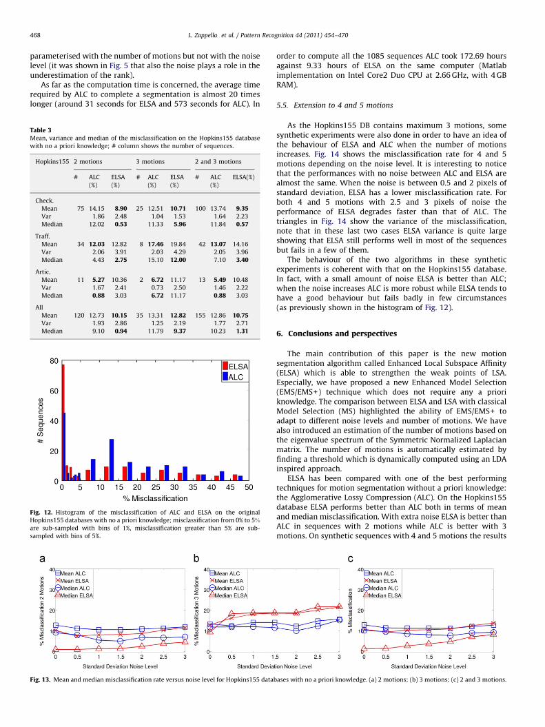
Table 3 shows mean, variance and median of the misclassifica-tion rate of ALC and ELSA on the original Hopkins155 databasedivided per number of motions and per type of sequence. Theoverall mean misclassification rate is similar for the twoalgorithms: 12.86% for ALC and 10.75% for ELSA. However, moreremarkable is the difference between the median values: themedian of ALC is 10.23% whereas the median of ELSA is only1.31%. This suggests that ELSA performs very well in most of thesequences and it fails only in a few of them. This is confirmed alsoby the results shown in Fig. 12 where the histogram of themisclassification is presented. From the histogram it is possible toappreciate that ELSA has more than 75 sequences with amisclassification rate between 0% and 1%, around 30 sequencesmore than ALC. ELSA has more sequences than ALC also in theranges 1–2% and 2–3%. The reason why ELSA is generally verygood, but when it fails the misclassification is very high, could beexplained by Fig. 3(i)–(p). From those plots it is possible to noticethat if the rank is not well estimated (especially if it isunderestimated) the affinity values quickly collapse to 1 or 0.When this happens the clustering process becomes very noisy,hence the segmentation result is greatly affected. ELSA alsoperforms better than ALC in terms of estimation of the number ofmotions. The mean errors (in absolute values) of the twoalgorithms are 1.16 for ALC and 0.36 for ELSA.

In Fig. 13 the trends of the mean and median misclassificationrate of ALC and ELSA when using the Hopkins155 database withextra noise are presented. The trends of both ALC and ELSA arevery stable showing that the algorithms are robust against noise.Mean and median performances of ELSA are always better thanthose of ALC with 2 motions. With 3 motions this is also truefor the original version of the database. When there are3 motions and high noise levels ALC is more robust than ELSA.This is probably due to the fact that the EMS+ correction is

pkins155 with extra noise; (b) 4 and 5 synthetic motions with noise.

L. Zappella et al. / Pattern Recognition 44 (2011) 454–470468

parameterised with the number of motions but not with the noiselevel (it was shown in Fig. 5 that also the noise plays a role in theunderestimation of the rank).

As far as the computation time is concerned, the average timerequired by ALC to complete a segmentation is almost 20 timeslonger (around 31 seconds for ELSA and 573 seconds for ALC). In

Table 3Mean, variance and median of the misclassification on the Hopkins155 database

with no a priori knowledge; # column shows the number of sequences.

Hopkins155 2 motions 3 motions 2 and 3 motions

# ALC

(%)

ELSA

(%)

# ALC

(%)

ELSA

(%)

# ALC

(%)

ELSA(%)

Check.

Mean 75 14.15 8.90 25 12.51 10.71 100 13.74 9.35Var 1.86 2.48 1.04 1.53 1.64 2.23

Median 12.02 0.53 11.33 5.96 11.84 0.57

Traff.

Mean 34 12.03 12.82 8 17.46 19.84 42 13.07 14.16

Var 2.06 3.91 2.03 4.29 2.05 3.96

Median 4.43 2.75 15.10 12.00 7.10 3.40

Artic.

Mean 11 5.27 10.36 2 6.72 11.17 13 5.49 10.48

Var 1.67 2.41 0.73 2.50 1.46 2.22

Median 0.88 3.03 6.72 11.17 0.88 3.03

All

Mean 120 12.73 10.15 35 13.31 12.82 155 12.86 10.75Var 1.93 2.86 1.25 2.19 1.77 2.71

Median 9.10 0.94 11.79 9.37 10.23 1.31

Fig. 12. Histogram of the misclassification of ALC and ELSA on the original

Hopkins155 databases with no a priori knowledge; misclassification from 0% to 5%

are sub-sampled with bins of 1%, misclassification greater than 5% are sub-

sampled with bins of 5%.

Fig. 13. Mean and median misclassification rate versus noise level for Hopkins155 datab

order to compute all the 1085 sequences ALC took 172.69 hoursagainst 9.33 hours of ELSA on the same computer (Matlabimplementation on Intel Core2 Duo CPU at 2.66 GHz, with 4 GBRAM).

5.5. Extension to 4 and 5 motions

As the Hopkins155 DB contains maximum 3 motions, somesynthetic experiments were also done in order to have an idea ofthe behaviour of ELSA and ALC when the number of motionsincreases. Fig. 14 shows the misclassification rate for 4 and 5motions depending on the noise level. It is interesting to noticethat the performances with no noise between ALC and ELSA arealmost the same. When the noise is between 0.5 and 2 pixels ofstandard deviation, ELSA has a lower misclassification rate. Forboth 4 and 5 motions with 2.5 and 3 pixels of noise theperformance of ELSA degrades faster than that of ALC. Thetriangles in Fig. 14 show the variance of the misclassification,note that in these last two cases ELSA variance is quite largeshowing that ELSA still performs well in most of the sequencesbut fails in a few of them.

The behaviour of the two algorithms in these syntheticexperiments is coherent with that on the Hopkins155 database.In fact, with a small amount of noise ELSA is better than ALC;when the noise increases ALC is more robust while ELSA tends tohave a good behaviour but fails badly in few circumstances(as previously shown in the histogram of Fig. 12).

6. Conclusions and perspectives

The main contribution of this paper is the new motionsegmentation algorithm called Enhanced Local Subspace Affinity(ELSA) which is able to strengthen the weak points of LSA.Especially, we have proposed a new Enhanced Model Selection(EMS/EMS+) technique which does not require any a prioriknowledge. The comparison between ELSA and LSA with classicalModel Selection (MS) highlighted the ability of EMS/EMS+ toadapt to different noise levels and number of motions. We havealso introduced an estimation of the number of motions based onthe eigenvalue spectrum of the Symmetric Normalized Laplacianmatrix. The number of motions is automatically estimated byfinding a threshold which is dynamically computed using an LDAinspired approach.

ELSA has been compared with one of the best performingtechniques for motion segmentation without a priori knowledge:the Agglomerative Lossy Compression (ALC). On the Hopkins155database ELSA performs better than ALC both in terms of meanand median misclassification. With extra noise ELSA is better thanALC in sequences with 2 motions while ALC is better with 3motions. On synthetic sequences with 4 and 5 motions the results

ases with no a priori knowledge. (a) 2 motions; (b) 3 motions; (c) 2 and 3 motions.

Fig. 14. Mean misclassification rate and variance versus noise level for synthetic experiments with no a priori knowledge. (a) 4 motions; (b) 5 motions.

L. Zappella et al. / Pattern Recognition 44 (2011) 454–470 469

where coherent with the ones obtained on the Hopkins155database: ELSA performs better than ALC with low noise levelsbut ALC is more robust when the noise increases. The maindrawback of ALC is the computation time, which is almost 20times longer than that required for ELSA.

To conclude, we discuss now some future directions ofresearch. As for future work connected with ELSA, we pointedout that we found a correlation between the number of motions,the noise and the position of the maximum entropy. It seems thatthe higher the number of motions and the noise level, the morethe entropy maximum tends to occur with a lower r. This hasbeen already shown with synthetic sequences and confirmed bythe fact that EMS+ performs better than EMS. However, a deeperstudy could reveal more useful ways of exploiting such acorrelation.

Nowadays the misclassification rates, assuming the number ofmotions is known, are already good. Despite the fact that themisclassification rates could be further improved we believe thatfuture work should focus on the ability to estimate the number ofmotions in a more efficient way. ALC and ELSA already providesatisfactory results without having this information, however,there is room for improvement especially when the motionsbecomes dependent. In general, feature-based techniques, such asmanifold clustering, have the advantage over dense-basedapproaches of reducing dramatically the computation. However,feature-based techniques have to rely on the ability of the trackerto find salient points and track them successfully throughout thevideo sequence. Nowadays, such an assumption is not tooconstraining but it is important to develop algorithms able todeal with only a few points (ideally from 5 to 7) per motioninstead of requiring lots of them. Moreover, another feature thatwe believe is very important in order to have a complete motionsegmentation system, useful in real time applications, is theability to work incrementally. An ideal incremental algorithmshould be able to refine the segmentation at every new frame (orevery small group of frames) without recomputing the wholesolution from the beginning.

Acknowledgements

This work has been supported by the Spanish Ministry ofScience projects DPI2007-66796-C03-02 and DPI2008-06548-C03-03/DPI. L. Zappella is supported by the Catalan governmentscholarship 2009FI_B1 00068. E. Provenzi acknowledges theRamon y Cajal fellowship by Ministerio de Ciencia y Tecnologıade Espana. The authors would like to thank the reviewers for theirvaluable and crucial comments.

Appendix A. Supplementary data

Supplementary data associated with this article can be foundin the online version at doi:10.1016/j.patcog.2010.08.015.

References

[1] A. Cavallaro, O. Steiger, T. Ebrahimi, Tracking video objects in clutteredbackground, IEEE Trans. Circuits Syst. Video Technol. 15 (4) (2005) 575–584.

[2] A. Colombari, A. Fusiello, V. Murino, Segmentation and tracking of multiplevideo objects, Pattern Recogn. 40 (4) (2007) 1307–1317.

[3] D. Cremers, S. Soatto, Motion competition: a variational approach topiecewise parametric motion segmentation, Int. J. Comput. Vision. 62 (3)(2005) 249–265.

[4] H. Shen, L. Zhang, B. Huang, P. Li, A map approach for joint motion estimation,segmentation, and super resolution, IEEE Trans. Image Process. 16 (2) (2007)479–490.

[5] N. Vaswani, A. Tannenbaum, A. Yezzi, Tracking deforming objects usingparticle filtering for geometric active contours, IEEE Trans. Pattern Anal.Machine Intell. 29 (8) (2007) 1470–1475.

[6] R. Stolkin, A. Greig, M. Hodgetts, J. Gilby, An em/e-mrf algorithm for adaptivemodel based tracking in extremely poor visibility, Image Vision Comput. 26(4) (2008) 480–495.

[7] L. Wiskott, Segmentation from motion: combining Gabor- and Mallat-wavelets to overcome aperture and correspondence problem, Lecture Notesin Computer Science, vol. 1296, 1997, pp. 329–336.

[8] M. Kong, J.-P. Leduc, B. Ghosh, V. Wickerhauser, Spatio-temporal continuouswavelet transforms for motion-based segmentation in real image sequences,IEEE Image Proc. 2 (1998) 662–666.

[9] L.M. Jos, A. Zuloaga, C. Cuadrado, J. Lzaro, U. Bidarte, Hardware implementa-tion of optical flow constraint equation using fpgas, Comput. Vis. Image Und.98 (3) (2005) 462–490.

[10] A. Bugeau, P. Perez, Detection and segmentation of moving objects incomplex scenes, Comput. Vis. Image Und. 113 (2009) 459–476.

[11] B. Ommer, T. Mader, J.M. Buhmann, Seeing the objects behind the dots:recognition in videos from a moving camera, Int. J. Comput. Vision 83 (2009)57–71.

[12] M.P. Kumar, P.H. Torr, A. Zisserman, Learning layered motion segmentationsof video, Int. J. Comput. Vision 76 (3) (2008) 301–319.

[13] C. Min, G. Medioni, Inferring segmented dense motion layers using 5dtensor voting, IEEE Trans. Pattern Anal. Machine Intell. 30 (9) (2008)1589–1602.

[14] J. Yan, M. Pollefeys, A general framework for motion segmentation:independent, articulated, rigid, non-rigid, degenerate and non-degenerate,Lecture Notes in Computer Science, vol. 3954, 2006, pp. 94–106.

[15] J. Yan, M. Pollefeys, A factorization-based approach for articulated nonrigidshape, motion and kinematic chain recovery from video, IEEE Trans. PatternAnal. Machine Intell. 30 (5) (2008) 865–877.

[16] L. Zappella, X. Llado, J. Salvi, Rank estimation of trajectory matrix in motionsegmentation, Electron. Lett. 45 (11) (2009) 540–541.

[17] R. Tron, R. Vidal, A benchmark for the comparison of 3-d motionsegmentation algorithms, in: Proceedings of CVPR IEEE, 2007, pp. 1–8.

[18] S.R. Rao, R. Tron, R. Vidal, Y. Ma, Motion segmentation via robust subspaceseparation in the presence of outlying, in: Proceedings of CVPR IEEE, 2008,pp. 1–8.

[19] L. Zappella, X. Llado, J. Salvi, New trends in motion segmentation, In-TECH(Ed.), Intechweb.org, 2009, pp. 31–46.

[20] T. Li, V. Kallem, D. Singaraju, R. Vidal, Projective factorization of multiplerigid-body motions, in: Proceedings of CVPR IEEE, 2007, pp. 1–6.

L. Zappella et al. / Pattern Recognition 44 (2011) 454–470470

[21] M.A. Fischler, R.C. Bolles, Ransac random sample consensus: a paradigm formodel fitting with applications to image analysis and automated cartogra-phy, Commun. ACM 24 (1981) 381–395.

[22] J. Ho, M.-H. Yang, J. Lim, K.-C. Lee, D. Kriegman, Clustering appearances ofobjects under varying illumination conditions, Proceedings of CVPR IEEE, vol.1, 2003, pp. 11–18.

[23] N.P. da Silva, J.P. Costeira, Subspace segmentation with outliers: a Grass-mannian approach to the maximum consensus subspace, in: Proceedings ofCVPR IEEE, 2008, pp. 1–6.

[24] K. Kanatani, C. Matsunaga, Estimating the number of independent motionsfor multibody motion segmentation, Proceedings of the Fifth ACCV, vol. 1,2002, pp. 7–12.

[25] K. Kanatani, Statistical optimization and geometric visual inference, in:Lecture Notes in Computer Science, 1997, pp. 306–322.

[26] Y. Sugaya, K. Kanatani, Geometric structure of degeneracy for multi-body motion segmentation, in: Lecture Notes in Computer Science, 2004,pp. 13–25.

[27] A. Gruber, Y. Weiss, Multibody factorization with uncertainty andmissing data using the em algorithm, Proceedings of CVPR IEEE, vol. 1,2004, pp. 707–714.

[28] A. Gruber, Y. Weiss, Factorization with uncertainty and missing data:exploiting temporal coherence, NIPS, vol. 16, MIT Press, Cambridge, MA, 2004.

[29] A. Gruber, Y. Weiss, Incorporating non-motion cues into 3d motionsegmentation, in: Lecture Notes in Computer Science, 2006, pp. 84–97.

[30] Y. Ma, H. Derksen, W. Hong, J. Wright, Segmentation of multivariate mixeddata via lossy data coding and compression, IEEE Trans. Pattern Anal.Machine Intell. 29 (9) (2007) 1546–1562.

[31] C. Tomasi, T. Kanade, Shape and motion from image streams under orthography:a factorization method, Int. J. Comput. Vision 9 (2) (1992) 137–154.

[32] J.P. Costeira, T. Kanade, A multibody factorization method for independentlymoving objects, Int. J. Comput. Vision 29 (3) (1998) 159–179.

[33] N. Ichimura, F. Tomita, Motion segmentation based on feature selection fromshape matrix, Syst. Comput. Jpn. 31 (4) (2000) 32–42.

[34] L. Zelnik-Manor, M. Irani, Degeneracies, dependencies and their implicationsin multi-body and multi-sequence factorizations, Proceedings of CVPR IEEE,vol. 2, 2003, pp. 287–293.

[35] H. Zhou, T.S. Huang, Recovering articulated motion with a hierarchicalfactorization method, Gesture Workshop, 2003, pp. 140–151.

[36] R. Vidal, R. Hartley, Motion segmentation with missing data usingpowerfactorization and gpca, Proceedings of CVPR IEEE, vol. 2, 2004,pp. 310–316.

[37] R. Vidal, R. Tron, R. Hartley, Multiframe motion segmentation with missing datausing powerfactorization and gpca, Int. J. Comput. Vision 79 (2008) 85–105.

[38] C. Julia, A. Sappa, F. Lumbreras, J. Serrat, A. Lopez, Rank estimation in 3dmultibody motion segmentation, Electron. Lett. 44 (4) (2008) 279–280.

[39] G. Chen, G. Lerman, Spectral curvature clustering (scc), Int. J. Comput. Vision81 (2009) 317–330.

[40] A. Goh, R. Vidal, Segmenting motions of different types by unsupervisedmanifold clustering, in: Proceedings of CVPR IEEE, 2007, pp. 1–6.

[41] L.K. Saul, S.T. Roweis, Think globally, fit locally: unsupervised learning of lowdimensional manifolds, J. Mach. Learn. Res. 4 (2003) 119–155.

[42] A. Goh, R. Vidal, Clustering and dimensionality reduction on riemannianmanifolds, in: Proceedings of CVPR IEEE, 2008, pp. 1–7.

[43] E. Elhamifar, R. Vidal, Sparse subspace clustering, in: Proceedings of CVPRIEEE, 2009, pp. 2790–2797.

[44] X. Llado, A.D. Bue, L. Agapito, Non-rigid metric reconstruction fromperspective cameras, Image Vision Comput. 28 (9) (2010) 1339–1353.

[45] S. Koterba, S. Baker, I. Matthews, C. Hu, J. Xiao, J.F. Cohn, T. Kanade, Multi-view aam fitting and camera calibration, in: ICCV, 2005, pp. 511–518.

[46] K. Kanatani, Motion segmentation by subspace separation and modelselection, IEEE Internat. Conf. Comput. Vision 2 (2001) 586–591.

[47] J. Shi, J. Malik, Normalized cuts and image segmentation, IEEE Trans. PatternAnal. Machine Intell. (2000) 888–905.

[48] J. Cheeger, A lower bound for the smallest eigenvalue of the laplacian,Problems in Analysis (1970) 195–199.

[49] A.V. Knyazev, M.E. Argentati, Principal angles between subspaces in an a-based scalar product: algorithms and perturbation estimates, SIAM J. Sci.Comput. 23 (6) (2002) 2008–2040.

[50] A. Bjorck, G.H. Golub, Numerical methods for computing angles betweenlinear subspaces, Math. Comput. 27 (123) (1973) 579–594.

[51] P.-A. Absil, A. Edelman, P. Koev, On the largest principal angle between randomsubspaces, Linear Algebra Appl. 414 (1) (2006) 288–294.

[52] L. Ambrosio, N. Gigli, G. Savare, Gradient flows in metric spaces and in the space ofprobability measures, in: Lectures in Mathematics, Birkhauser, 2005.

[54] F. Chung, Spectral Graph Theory, CBMS Regional Conference Series inMathematics, vol. 92, American Mathematical Society, 1997.

[55] U. von Luxburg, A tutorial on spectral clustering, Statist. Comput. 17 (4)(2007) 395–416.

[56] J.C. Bezdek, Pattern Recognition with Fuzzy Objective Function Algorithms,Kluwer Academic Publishers, Norwell, MA, USA, 1981.

[57] N. Otsu, A threshold selection method from gray-level histograms, IEEE Trans.Syst. Man Cybern. 9 (1) (1979) 62–66.

L. Zappella received his MSc degree in Computer Science at the University of Milan at the end of 2003. He received the European MSc degree in Computer Vision andRobotics (VIBOT) in 2008. Currently, he is completing his PhD at the University of Girona. His research interests are in d image processing and computer vision, with specificfocus on motion segmentation and structure from motion.

X. Llado received the B.S. degree in Computer Science in 1999, and the PhD in Computer Engineering in 2004. Currently, he is a lecturer at the University of Girona. Hisresearch interests are in the field of image processing and computer vision, focusing on colour and texture analysis, shape from shading, and structure from motion.

Edoardo Provenzi received the degree in Physics at Universit�a di Milano, Italy, in 2000 and the PhD in Mathematics and applications at Universit�a di Genova, Italy, in 2003.He is currently a post-doc Ramon y Cajal researcher at Universitat Pompeu Fabra in Barcelona, Spain, in the field of computer vision, with particular interest inmathematical models of color image processing.

J. Salvi graduated in Computer Science at the Technical University of Catalonia in 1993, received the MSc in Computer Science in July 1996 and the PhD in IndustrialEngineering in 1998 both at the University of Girona, Spain. He is currently an associate professor and a senior researcher at the Computer Vision and Robotics Group,University of Girona.